solution guide for chapter 3: straight lines and linear...
TRANSCRIPT

Solution Guide for Chapter 3:Straight Lines andLinear Functions
3.1 THE GEOMETRY OF LINES
E-1 An alternative version of similarity: We know from Euclidean geometry theorem 2 that
if ∆ABC is similar to ∆A′B′C ′ then
|AB||A′B′|
=|AC||A′C ′|
.
Multiplying both sides by |A′B′| and dividing both sides by |AC| gives
|AB||AC|
=|A′B′||A′C ′|
,
as desired.
E-2 Two-angle criterion for similarity: Let the angles of the first triangle have measure α, β,
and γ, and let the angles of the other triangle have measure α′, β′, and γ′, chosen so that
the two congruence relations correspond to α = α′ and β = β′. (We measure all angles
in degrees.) We want to show that γ = γ′. Now by Euclidean geometry theorem 1 we
have
α + β + γ = 180
and
α′ + β′ + γ′ = 180.
Solving for γ in the first equation gives
γ = 180− α− β,
and solving for γ′ in the second gives
γ′ = 180− α′ − β′.
Because α = α′ and β = β′, we find
γ = 180− α− β = 180− α′ − β′ = γ′.
SECTION 3.1 The Geometry of Lines 225
Thus γ = γ′. Hence the two triangles have congruent angles, and they are similar, as
desired.
E-3 Calculating with similarity: By Euclidean geometry theorem 2 we have105
=a
6, and
multiplying both sides by 6 gives a = 12. Applying the theorem again gives510
=b
6,
and multiplying both sides by 6 gives b = 3.
E-4 Defining the sine function: First we show that the triangles ∆CAB and ∆EAD are
similar. In fact, they share the angle A, and both have a right angle, so by the two-
angle criterion in Exercise E-2 the triangles are similar. Now we use Euclidean geometry
theorem 2:|BC||DE|
=|AC||AE|
.
Multiplying both sides by |DE| and dividing both sides by |AC| gives
|BC||AC|
=|DE||AE|
,
as desired.
E-5 The Pythagorean theorem:
(a) First we show that the triangles ∆ABC and ∆DAC are similar. In fact, they share
an angle at C, and both have a right angle, so by the two-angle criterion in Exercise
E-2 the triangles are similar. Next we show that the triangles ∆ABC and ∆DBA
are similar. In fact, they share an angle at B, and both have a right angle, so by the
two-angle criterion in Exercise E-2 the triangles are similar.
(b) Because ∆ABC and ∆DAC are similar, by Euclidean geometry theorem 2 we have
|BC||AC|
=|AC||DC|
,
which says thatc
a=
a
d.
Multiplying both sides by ad gives cd = a2, as desired.
(c) Because ∆ABC and ∆DBA are similar, by Euclidean geometry theorem 2 we have
|BC||BA|
=|AB||DB|
,
which says thatc
b=
b
e.
Multiplying both sides by be gives ce = b2, as desired.

226 Solution Guide for Chapter 3
(d) By Parts (b) and (c) we have the equations cd = a2 and ce = b2. Adding these
equations gives
a2 + b2 = cd + ce.
Now d + e = c because the length of the line segment BC is the sum of the lengths
of DC and BD. Thus
cd + ce = c(d + e) = c(c) = c2.
Combining the last two displayed equations yields a2 + b2 = c2, as desired.
E-6 Another proof of the Pythagorean theorem: Behold!
The two squares in Figure 3.29 have total area a2 + b2, and (as noted in the text) the
square in Figure 3.28 has area c2. This rearrangement shows that a2 + b2 = c2.
E-7 A right triangle: First we find the slope of the line passing through (1, 1) and (3, 4). We
have
Slope =Vertical change
Horizontal change=
4− 13− 1
=32.
Next we find the slope of the line passing through (1, 1) and (4,−1). We have
Slope =Vertical change
Horizontal change=−1− 14− 1
=−23
.
Because the slope −23
is the negative reciprocal of the slope32
, the two lines are perpen-
dicular. Hence the given points do form the vertices of a right triangle.

SECTION 3.1 The Geometry of Lines 227
E-8 Parallel and perpendicular lines:
(a) Solving the first equation for y gives y = −32x+2, so the slope of the first line is−3
2.
Solving the second equation for y gives y = −32x +
94
, so the slope of the second
line is −32
also. Because the slopes are the same, the lines are parallel.
(b) Solving the first equation for y gives y =57x − 3
7, so the slope of the first line is
57
. Solving the second equation for y gives y =43x − 8
3, so the slope of the second
line is43
. Because the slopes are not the same, the lines are not parallel. Because
the slopes are not negative reciprocals of each other, the lines are not perpendicular.
Hence the lines are neither parallel nor perpendicular.
(c) Solving the first equation for y gives y = −57x +
157
, so the slope of the first line
is −57
. Solving the second equation for y gives y =75x +
715
, so the slope of the
second line is75
. Because the slopes are negative reciprocals of each other, the lines
are perpendicular.
(d) Solving the first equation for y gives y = −a
bx +
c
b, so the slope of the first line is
−a
b. Solving the second equation for y gives y = −a
bx +
d
bk, so the slope of the
second line is −a
b. Because the slopes are the same, the lines are parallel.
E-9 A system of equations with no solution: Solving the first equation for y gives y =
−27x +
97
, so the slope of the first line is −27
. Solving the second equation for y gives
y = −27x +
514
, so the slope of the second line is −27
also. Because the slopes are the
same, the lines are parallel. Evidently, though, the lines have different vertical intercepts,
so they are not coincident (that is, not the same). Thus the graphs represented by the two
linear equations do not cross. Hence the system has no solution.
S-1. Slope from rise and run: We have Slope =RiseRun
. In this case, the rise is 8 feet, the
height of the wall, and the run is 2 feet, since that is the horizontal distance from the
wall. Thus the slope is82
= 4 feet per foot.
S-2. Slope from rise and run: We have Slope =RiseRun
. In this case, the rise is 15 feet, the
height of the wall, and the run is 3 feet, since that is the horizontal distance from the
wall. Thus the slope is153
= 5 feet per foot.

228 Solution Guide for Chapter 3
S-3. Height from slope and horizontal distance: We have
Vertical change = Slope × Horizontal change.
In this case, the slope of the ladder is 2.5, while the horizontal distance is 3 feet, so the
vertical height is 2.5× 3 = 7.5 feet.
S-4. Height from slope and horizontal distance: We have
Vertical change = Slope × Horizontal change.
In this case, the slope of the ladder is 1.7, while the horizontal distance is 4 feet, so the
vertical height is 1.7× 4 = 6.8 feet.
S-5. Horizontal distance from height and slope: We have
Vertical change = Slope × Horizontal change.
In this case, the slope of the ladder is 1.75, while the vertical distance is 9 feet, so we
have 9 = 1.75× Horizontal change. Thus the horizontal distance is9
1.75= 5.14 feet.
S-6. Horizontal distance from height and slope: We have
Vertical change = Slope × Horizontal change.
In this case, the slope of the ladder is 2.1, while the vertical distance is 12 feet, so we
have 12 = 2.1× Horizontal change. Thus the horizontal distance is122.1
= 5.71 feet.
S-7. Slope from two points: We have Slope =Vertical change
Horizontal change. In this case, the vertical
change is −2 feet (12 feet dropped to 10 feet) while the horizontal change is 3 feet (since
west is the positive direction). Thus the slope is−23
= −23
foot per foot.
S-8. Continuation of Exercise S-7: We have Vertical change = Slope × Horizontal change.
In this case, the slope is −23
, while the horizontal change is 5, since I move 5 additional
feet west. Thus the vertical change is −23× 5 = −3.33 feet, and so the height of the roof
is now 10− 3.33 = 6.67 feet.
S-9. A circus tent: We have Vertical change = Slope × Horizontal change. In this case, the
slope is −0.8, while the horizontal change is 7 feet, so the vertical change is −0.8 × 7 =
−5.6 feet. Thus the height of the tent if I walk 7 feet west is 22− 5.6 = 16.4 feet.

SECTION 3.1 The Geometry of Lines 229
S-10. More on the circus tent: We have Vertical change = Slope × Horizontal change. In this
case, the slope is −0.8 and the vertical change is −22 feet (22 feet dropped to 0 feet, for a
change of −22 feet), so we have −22 = −0.8 × Horizontal change. Thus the horizontal
change is−22−0.8
= 27.5 feet. Thus it is 27.5 feet from the center of the tent to where the
roof meets the ground.
S-11. Slope: We have Slope =RiseRun
. In this case, the rise is 100 feet, the height of the building,
and the run is 70 feet, since that is the horizontal distance to the building. Thus the slope
is10070
= 1.43 feet per foot.
S-12. Vertical distance from length and slope: We have
Vertical change = Slope × Horizontal change.
In this case, the slope of the line is 1.8, while the horizontal distance is 130 feet, so the
vertical height is 1.8× 130 = 234 feet.
1. A line with given intercepts: The picture is drawn below. Since the line is falling from
left to right, we expect the slope of the line to be negative. The slope is
m =Vertical change
Horizontal change=
0− 43− 0
= −43.
2. A line with given vertical intercept and slope: To make the graph, we start with the
vertical intercept at 3 and draw a line with slope 1. That is, the line should rise one unit
for each unit of run. Our graph is shown below.
To find the horizontal intercept, we need to know how far to the left we should move
to make the graph fall 3 units. Since the graph rises by 1 unit for each unit of run, we
need to move 3 units to the left to get to the horizontal intercept. Thus the horizontal
intercept is at −3.

230 Solution Guide for Chapter 3
3. Another line with given vertical intercept and slope: Because the graph falls by 2
units for each unit of run, we need to move82
= 4 units to the right of the vertical axis
to get to the horizontal intercept. Thus the horizontal intercept is 4. More formally, if
we move from the location of the horizontal intercept to that of the vertical, we have
Slope =Vertical change
Horizontal change=
Vertical intercept− 00− Horizontal intercept
,
so
−2 =8
− Horizontal intercept,
and solving gives the value of 4 for the horizontal intercept.
4. A line with given horizontal intercept and slope: The graph rises by 3 units for each
unit of run, and we need to move 6 units to the left of the horizontal intercept to get to
the vertical axis. Thus the vertical intercept is−6×3 = −18. More formally, if we move
from the location of the horizontal intercept to that of the vertical intercept, we have
Slope =Vertical change
Horizontal change=
Vertical intercept− 00− Horizontal intercept
,
so
3 =Vertical intercept
−6,
and multiplying both sides by −6 gives the value of −18 for the vertical intercept.
5. Lines with the same slope: The first line should have a vertical intercept at 3 and rise
2 units for each unit of run. The second should have a vertical intercept of 1 and rise 2
units for each unit of run. Our picture is shown below. The lines do not cross. Different
lines with the same slope are parallel.

SECTION 3.1 The Geometry of Lines 231
6. Where lines with different slopes meet: One line should cross the vertical axis at 2
and rise 3 units for each unit of run. The other should cross the vertical axis at 4 and
rise 1 unit for each unit of run. Our picture is shown below. These two lines cross to
the right of the vertical axis. For the two lines to cross to the right of the vertical axis,
the slope of the line with the lower vertical intercept must be greater than the slope of
the line with the higher vertical intercept.
7. A ramp to a building:
(a) The slope of the graph is 0.4, so one foot of run results in 0.4 foot of rise. Thus, one
foot from the base of the ramp, it is 0.4 foot high.
(b) To get to the steps we have moved horizontal 15 feet from the base of the ramp.
Since the slope is 0.4, the ramp rises
Rise = Run × Slope = 15× 0.4 = 6 feet.
8. A wheelchair service ramp:
(a) Since the slope of the ramp has to be112
, we know that for every horizontal foot we
move, we rise112
vertical foot. The rise we need is 2 feet, or 24 increments of112
.
That means we need to start the ramp 24 feet away from the steps. Alternatively,
we can do this with a formula:
Rise = Run × Slope
2 = Run × 112
24 = Run Multiply both sides by 12.
(b) One foot of run allows112
foot of rise. That is one inch. Thus the allowable rise is
one inch for 1 foot of run.
9. A cathedral ceiling:
(a) When we move 3 feet east from the west wall, the ceiling rises 10.5 − 8 = 2.5. So
the slope is
Slope =RiseRun
=2.53
= 0.83 foot per foot.
232 Solution Guide for Chapter 3
(b) If we move 17 feet to the right of the west wall then the vertical change is
Rise = Slope × Run = 0.83× 17 = 14.11 feet.
So the height of the ceiling at that point is 8 + 14.11 = 22.11 feet.
(c) Since we start at 8 feet high on the west wall and we want to reach a 12-foot height,
then the vertical change is 4 feet. Now
Vertical change = Horizontal change × Slope
4 = Horizontal change × 0.834
0.83= Horizontal change Divide both sides by 0.83.
4.82 = Horizontal change.
So if we place the light 4.82 feet from the west wall, then we will still be able to
change the bulb.
10. Roof trusses: In both parts we focus on the part of the roof line sloping upward from
left to right, and we take movement toward the center as going in the positive direction.
Moving along this line from the outer wall to the peak, we have a horizontal change of
8 feet (half the length of the joist) and a vertical change of 4 feet. Thus the slope of this
line is48
= 0.5 foot per foot.
(a) Moving along the line from the outer wall to the vertical strut, we have a horizon-
tal change of 3 feet, and the vertical change is the length of the strut. Because the
slope is 0.5, from
Vertical change = Slope × Horizontal change,
we find
Vertical change = 0.5× 3 = 1.5 feet.
Thus the length of the strut is 1.5 feet.
(b) Moving from the tip of the rafter to the top of the wall, we have a horizontal
change of 1.5 feet. Because the slope is 0.5, from
Vertical change = Slope × Horizontal change,
we find
Vertical change = 0.5× 1.5 = 0.75 foot.
Thus the outside tip is 8− 0.75 = 7.25 feet above the floor.

SECTION 3.1 The Geometry of Lines 233
11. Cutting plywood siding: The shape of the first piece shows that for a horizontal change
(to the left) of 4 feet the vertical change along the roof line is 2.5 − 1 = 1.5 feet. Now
each piece has width 4 feet, so we observe that for each piece the longer side and the
shorter side differ in length by 1.5 feet.
(a) By the observation above, the length h is 2.5 + 1.5 = 4 feet.
(b) By the observation above, the length k is h + 1.5 = 4 + 1.5 = 5.5 feet, or 5 feet 6
inches.
Alternative approach: In both parts we focus on the part of the roof line sloping
upward from right to left, and we take movement toward the center as going in
the positive direction. Moving along this line from the outer wall to the far corner
of the first piece of siding, we have a horizontal change of 4 feet and a vertical
change of 2.5− 1 = 1.5 feet. Thus the slope of this line is1.54
= 0.375 foot per foot.
For Part(a): Moving along upper edge of the second piece of siding toward the
peak, we have a horizontal change of 4 feet. Because the slope is 0.375, from
Vertical change = Slope × Horizontal change,
we find
Vertical change = 0.375× 4 = 1.5 feet.
To find h we add this vertical change to the length 2.5 feet of the short side of the
second piece. Thus the length h is 2.5 + 1.5 = 4 feet.
For Part(b): Moving along upper edge of the third piece of siding toward the peak,
we have a horizontal change of 4 feet. Because the slope is 0.375, from
Vertical change = Slope × Horizontal change,
we again find
Vertical change = 0.375× 4 = 1.5 feet.
To find k we add this vertical change to the length 4 feet of the short side of the
third piece. Thus the length h is 4 + 1.5 = 5.5 feet.
12. An overflow pipeline: Because a 12-foot stretch represents1296
=18
of the entire hori-
zontal distance of 96 feet, over a 12-foot horizontal stretch the pipe drops by 5× 18
=58
foot, or about 0.63 foot. An alternative approach is to compute the slope as596
(with
the proper choice of direction) and to conclude that the vertical change is596× 12 =
58
foot.

234 Solution Guide for Chapter 3
13. Looking over a wall: Assuming that the man can just see the top of the building over
the wall, we focus on the line of sight from the man to the top of the building. Taking
south as the positive direction, we compute the slope of the line by considering the
change from the top of the wall to the top of the building. We find that the slope of the
line is
Slope =Vertical change
Horizontal change=
50− 3520
=1520
= 0.75 foot per foot.
Now we find the horizontal distance from the wall to the man by considering the
change along the line from the man to the top of the wall. We use
Vertical change = Slope × Horizontal change,
which says
35− 6 = 0.75× Horizontal distance.
Dividing both sides by 0.75 shows that the horizontal distance is35− 60.75
= 38.67 feet.
Thus the man must be at least 38.67 feet north of the wall.
14. The Mississippi River:
(a) Since the Gulf of Mexico is at sea level, or 0 feet above sea level, then the vertical
change from Lake Itasca to the Gulf of Mexico is 0− 1475 = −1475 feet. Note that
the change is negative, since the river is decreasing in elevation as it flows south.
The horizontal change is 2340 miles. So the slope is
Vertical changeHorizontal change
=−14752340
= −0.63 foot per mile.
Thus, the river drops about 0.63 foot per mile. (If all distances are converted to
feet, then the slope is −0.00012 foot per foot.)
(b) The vertical change in going from Lake Itasca to Memphis is calculated as
Vertical change = Horizontal change × Slope = 1982×−0.63 = −1248.66 feet.
Since we started at 1475 feet, the elevation of the river at Memphis is 1475 −
1248.66 = 226.34 feet.
(c) The vertical change in going from 1475 feet to 200 feet is −1275 feet.
Vertical change = Horizontal change × Slope
−1275 = Horizontal change ×−0.63−1275−0.63
= Horizontal change Divide each side by −0.63.
2023.81 = Horizontal change.

SECTION 3.1 The Geometry of Lines 235
So we would expect the elevation of the river to be 200 feet when we are 2023.81
miles south of Lake Itasca.
15. A road up a mountain:
(a) The vertical change is 4960− 4130 = 830 feet. The horizontal change is 3 miles. So
the slope isVertical change
Horizontal change=
8303
= 276.67 feet per mile.
(b) The vertical change in moving 5 miles from the first sign is
Rise = Run × Slope = 5× 276.67 = 1383.35 feet.
Since we started at 4130 feet at the first sign, the elevation is 4130 + 1383.35 =
5513.35 feet when we are five miles from the first sign.
(c) The vertical change from the first sign to the peak is 10, 300− 4130 = 6170 feet.
Vertical change = Horizontal change × Slope
6170 = Horizontal change × 276.676170
276.67= Horizontal change Divide both sides by 276.67.
22.30 = Horizontal change.
Thus the peak is 22.30 horizontal miles away.
16. An underground water source:
(a) Since the limestone layer drops from 220 to 270 feet from 2 to 3 miles, the layer
drops 50 feet each mile west of Seiling.
The horizontal change in going from 2 miles to 5 miles west of Seiling is 3 miles.
Thus the vertical change is 3× 50 = 150 feet. Since we started at a 220 foot depth,
the limestone should be 220+150 = 370 feet deep 5 miles west of Seiling.
(b) The vertical change from 220 feet to 290 feet is 70. So the horizontal change is7050
= 1.4 miles. We started 2 miles from Seiling to begin with (where the limestone
is 220 feet deep), so we can drill the well at most 3.4 miles west of Seiling.
(c) Now 3 miles west of Seiling the limestone layer is 270 feet deep . If we went one
more mile west we would expect the limestone to be 270 + 50 = 320 feet deep if
it followed a straight line. But it is only 273 feet deep. So the hydrologists were
incorrect in their assumption that the limestone followed a straight line.

236 Solution Guide for Chapter 3
17. Earth’s umbra: We take the positive horizontal axis to pass from the point where the
umbra ends through the center of Earth. We find the slope of the upper line shown
in the figure by considering the change from the point where the umbra ends to the
surface of Earth. We find that the slope is
Slope =Vertical change
Horizontal change=
Radius of EarthDistance from Earth to end of umbra
=3960
860,000mile per mile.
Now we find the radius of the umbra at the indicated point by considering the change
along the line from the point where the umbra ends to the radius at the indicated point.
We use
Vertical change = Slope × Horizontal change.
Now the vertical change is the radius of the umbra we are asked to find, and the hor-
izontal change is 860,000 − 239,000 = 621,000. Using the slope calculated above, we
find
Radius of the umbra =3960
860,000× 621,000 = 2859.49 miles.
Thus the radius of the umbra at the indicated point is about 2859 miles. Since the
radius of the moon is smaller than this, the moon can fit inside Earth’s umbra. When
this happens there is a total lunar eclipse.
18. The Earth’s penumbra: We take the positive horizontal axis to pass from the apex
through the center of Earth. We find the slope of the upper line shown in the figure by
considering the change from the surface of Earth to the point where the penumbra has
a radius of 10,000 miles. We find that the slope is
Slope =Vertical change
Horizontal change=
10,000− Radius of EarthDistance from Earth to the moon
.
Thus we have
Slope =10,000− 3960
239,000=
6040239,000
mile per mile.
Now we find the distance from Earth to the apex by considering the change from the
apex to the surface of Earth. We use
Vertical change = Slope × Horizontal change.
Now the vertical change is the radius of Earth, and the horizontal change is the distance
we are asked to find. Using the slope calculated above, we find
3960 =6040
239,000× Distance,
and when we solve this equation we find that the distance is 156,695.36 miles. Thus the
apex is about 156,695 miles from Earth.
SECTION 3.2 Linear Functions 237
19. The umbra of the moon: We take the positive horizontal axis to pass from the apex (at
the center of Earth) to the center of the sun. We find the slope of the line from the apex
to the surface of the sun by considering the change from the apex to the surface of the
moon. (This can be visualized by replacing Earth by the moon in Figure 3.40.) We find
that the slope is
Slope =Vertical change
Horizontal change=
Radius of moonDistance from Earth to moon
=1100
239,000mile per mile.
Now we find the radius of the sun by considering the change from the apex to the
surface of the sun. We use
Vertical change = Slope × Horizontal change.
Now the vertical change is the desired radius of the sun, and the horizontal change is
the distance from Earth to the sun. Using the slope calculated above, we find
Radius of the sun =1100
239,000× 93,498,600 = 430,328.28 miles.
Thus the radius of the sun is about 430,328 miles.
3.2 LINEAR FUNCTIONS
E-1. Parallel lines: We know from the preceding section that parallel lines have the same
slope. The line y = 3x − 2 has slope 3, so we want to find the equation of the line with
slope 3 that passes through the point (3, 3). We use the point-slope form:
y − 3 = 3(x− 3)
y − 3 = 3x− 9
y = 3x− 6.
E-2. Perpendicular lines: The line y = 4x + 1 has slope 4, so, by the preceding section, any
line perpendicular to the given line has slope −14
. Hence we want to find the equation
of a line with slope−14
that passes through the point (8, 2). We use the point-slope form:
y − 2 = −14(x− 8)
y − 2 = −14x + 2
y = −14x + 4.

238 Solution Guide for Chapter 3
E-3. Finding equations of lines:
(a) We use the point-slope form:
y − 1 = 3(x− 2)
y − 1 = 3x− 6
y = 3x− 5.
(b) We use the point-slope form:
y − 1 = −4(x− 1)
y − 1 = −4x + 4
y = −4x + 5.
(c) We use the two-point form. We have
y − 2 =(
10− 25− 1
)(x− 1)
y − 2 = 2x− 2
y = 2x.
(d) We use the two-point form. We have
y − 1 =(
2− 1−2− 3
)(x− 3)
y − 1 = −15x +
35
y = −15x +
85.
E-4. Finding the equation of a line: The slope of the line 3x+2y = 4 can be found by putting
the line in standard form:
3x + 2y = 4
2y = −3x + 4
y = −32x + 2.
Thus the line has slope−32
. We know from the preceding section that parallel lines have
the same slope, so the line we are looking for has slope −32
also.
The horizontal intercept of the line 2x − y = 8 can be found by putting in y = 0 and
solving for x. Thus we have
2x− 0 = 8
2x = 8
x = 4.

SECTION 3.2 Linear Functions 239
Thus the horizontal intercept is 4. This means that the line we are looking for passes
through the point (4, 0).
Thus we are looking for a line with slope −32
that passes through the point (4, 0). We
use the point-slope form:
y − 0 = −32(x− 4)
y = −32x + 6.
Thus the equation is y = −32x + 6.
S-1. Slope from two values: We have that the slope m is:
m =Change in functionChange in variable
=19− 75− 2
=123
= 4.
S-2. Slope from two values: We have that the slope m is:
m =Change in functionChange in variable
=9− 53− 8
=4−5
= −0.8.
S-3. Function value from slope and run: We have that the slope is m = 2.7:
2.7 =Change in functionChange in variable
=f(5)− f(3)
5− 3=
f(5)− 75− 3
=f(5)− 7
2.
Thus f(5)− 7 = 2× 2.7 = 5.4, and so f(5) = 5.4 + 7 = 12.4.
S-4. Function value from slope and run: We have that the slope is m = 3.1:
3.1 =Change in functionChange in variable
=f(12)− f(5)
12− 5=
f(12)− 212− 5
=f(12)− 2
7.
Thus f(12)− 2 = 7× 3.1 = 21.7, and so f(12) = 21.7 + 2 = 23.7.
S-5. Run from slope and rise: We have that the slope is m = −3.4:
−3.4 =Change in functionChange in variable
=f(x)− f(1)
x− 1=
0− 6x− 1
=−6
x− 1.
Thus −6 = −3.4× (x− 1), so x− 1 =−6−3.4
= 1.76, and therefore x = 1.76 + 1 = 2.76.
S-6. Run from slope and rise: We have that the slope is m = 2.6:
2.6 =Change in functionChange in variable
=f(x)− f(5)
x− 5=
0− (−3)x− 5
=3
x− 5.
Thus 3 = 2.6× (x− 5), so x− 5 =3
2.6= 1.15, and therefore x = 1.15 + 5 = 6.15.

240 Solution Guide for Chapter 3
S-7. Linear equation from slope and point: Since f is a linear function with slope 4, f =
4x+ b for some b. Now f(3) = 5, so 5 = 4× 3+ b, and therefore b = 5− 4× 3 = −7. Thus
f = 4x− 7.
S-8. Linear equation from slope and point: Since f is a linear function with slope −3, f =
−3x + b for some b. Now f(2) = 8, so 8 = −3× 2 + b, and therefore b = 8 + 3× 2 = 14.
Thus f = −3x + 14.
S-9. Linear equation from two points: We first compute the slope:
m =Change in functionChange in variable
=f(9)− f(4)
9− 4=
2− 89− 4
=−65
= −1.2.
Since f is a linear function with slope −1.2, f = −1.2x + b for some b. Now f(4) = 8, so
8 = −1.2× 4 + b, and therefore b = 8 + 1.2× 4 = 12.8. Thus f = −1.2x + 12.8.
S-10. Linear equation from two points: We first compute the slope:
m =Change in functionChange in variable
=f(7)− f(3)
7− 3=−4− 57− 3
=−94
= −2.25.
Since f is a linear function with slope −2.25, f = −2.25x + b for some b. Now f(3) = 5,
so 5 = −2.25× 3 + b, and therefore b = 5 + 2.25× 3 = 11.75. Thus f = −2.25x + 11.75.
S-11. Linear equation from slope and points: We are given the slope m = −1.7 and the initial
value b = −3.7 (because f(0) = −3.7). Thus f = −1.7x− 3.7.
S-12. Linear equation from slope and points: Since f is a linear function with slope −1.7,
f = −1.7x + b for some b. Now f(−1) = −3.7, so −3.7 = −1.7× (−1) + b, and therefore
b = −3.7 + 1.7× (−1) = −5.4. Thus f = −1.7x− 5.4.
S-13. Linear equation from two points: We first compute the slope:
m =Change in functionChange in variable
=f(0)− f(−2)
0− (−2)=
3− 22
=12
= 0.5.
Now we need the initial value b. Since f(0) = 3, that value is b = 3. Thus f = 0.5x + 3.
S-14. Linear equation from two points: We first compute the slope:
m =Change in functionChange in variable
=f(2)− f(−2)
2− (−2)=
3− 24
=14
= 0.25.
Since f is a linear function with slope 0.25, f = 0.25x + b for some b. Now f(−2) = 2, so
2 = 0.25× (−2) + b, and therefore b = 2− 0.25× (−2) = 2.5. Thus f = 0.25x + 2.5.

SECTION 3.2 Linear Functions 241
1. Getting Celsius from Fahrenheit:
(a) Water freezes at 0 degrees Celsius, which is 32 degrees Fahrenheit. So C = 0 when
F = 32. Water boils at 100 degrees Celsius, which is 212 degrees Fahrenheit. So
C = 100 when F = 212. These two bits of information allow us to get the slope of
the function:
Slope =Change in C
Change in F=
100− 0212− 32
= 0.56.
Thus C = 0.56F + b, and we need to find b. When C = 0, then F = 32. This gives
0 = 0.56× 32 + b. Solving for b, we get b = −17.92. Thus C = 0.56F − 17.92.
There are some variations that yield slightly different formulas. The differences
are due to the rounding of59
as 0.56. If the fraction is left as a fraction, then the
formula will be C =59F − 160
9, which, to two decimal places, is C = 0.56F −
17.78. If the second data point, C = 100 when F = 212, is used to find b from
C = 0.56F + b, the resulting calculation will yield b = −18.72, giving the formula
C = 0.56F − 18.72.
(b) The slope we found in Part (a) was 0.56. This means that for every one degree
increase in the Fahrenheit temperature, the Celsius temperature will increase by
0.56 degree.
(c) We need to solve F = 1.8C + 32 for C. We have
F = 1.8C + 32
F − 32 = 1.8C Subtract 32 from each side.1
1.8× (F − 32) = C Divide both sides by 1.8.
11.8
F − 11.8
× 32 = C
0.56F − 17.78 = C
This is the same as the formula we found in Part (a).
2. A trip to a science fair:
(a) Now
Cost = Cost of admission + Bus cost
C = $2 per student × Number of students + $130
C = 2n + 130 dollars.
(b) The slope is 2, and the vertical intercept is 130. The slope indicates that for each
additional child we take on the trip the total cost increases by $2. The initial value
is $130, and it is the cost of taking the bus itself to the fair.

242 Solution Guide for Chapter 3
(c) Here C(5) represents the total cost (in dollars) of the science fair trip if 5 children
make the trip. Its value is C(5) = 2× 5 + 130 = 140 dollars.
(d) We have
2n + 130 = 146
2n = 16 Subtract 130 from each side.
n = 8 Divide both sides by 2.
The solution of the equation 2n+130 = 146 is the number of students we can take
if there is $146 to spend. We found that we can take only 8 students for $146.
3. Digitized pictures on a disk drive:
(a) Each additional picture stored increases the total storage space used by 2 megabytes.
This means that the change in total storage space used is always the same, 2
megabytes, for a change of 1 in the number of pictures that are stored. Thus the
storage space used S is a linear function of the number of pictures stored n.
(b) From Part (a), S is a linear function of n with slope 2, since the slope represents the
additional storage space used with the addition of 1 picture. The initial value of S
is the amount of storage space used if n = 0, that is, if no pictures are stored. Since
the formatting information, operating system, and applications software use 6000
megabytes, that is the initial value. Thus a formula for S(n) is S = 2n + 6000.
(c) The total amount of storage space used on the disk drive if there are 350 pictures
stored on the drive is expressed in functional notation as S(350). (Of course, this
depends on the choice of function name we made in Part (b).) Its value is S(350) =
2× 350 + 6000 = 6700 megabytes.
(d) If there are 769,000 megabytes free and the drive holds 800,000 megabytes, then
there are 800,000 − 769,000 = 31,000 megabytes used. To find out how many
pictures are stored, we need to solve this equation for n:
2n + 6000 = 31,000
2n = 31,000− 6000 = 25,000 Subtract 6000 from both sides.
n =25,000
2= 12,500 pictures Divide both sides by 2.
Thus there are 12,500 digitized pictures stored. There are 769,000 megabytes of
room left, and that space can hold769,000
2= 384,500 more pictures before the
disk drive is full.
SECTION 3.2 Linear Functions 243
4. Speed of sound:
(a) Because S always increases by 1.1 when T increases by 1, S has a constant rate of
change and so is a linear function of T . The slope is the constant rate of change,
namely 1.1 feet per second per degree.
(b) We know that the slope is 1.1, so S = 1.1T + b for some constant b. We find b
using the fact that S = 1087.5 when T = 32: We have 1087.5 = 1.1 × 32 + b, so
b = 1087.5− 1.1× 32 = 1052.3. Thus the formula is S = 1.1T + 1052.3.
(c) We need to solve S = 1.1T + 1052.3 for T . We have
S = 1.1T + 1052.3
S − 1052.3 = 1.1T Subtract 1052.3 from each side.S − 1052.3
1.1= T Divide both sides by 1.1.
Thus T =S − 1052.3
1.1. Dividing through by 1.1 gives T = 0.91S − 956.64.
(d) The slope of T as a linear function of S is 0.91, and this means that an increase in
the speed of sound by 1 foot per second corresponds to an increase of 0.91 degree
in temperature.
5. Total cost:
(a) Because the variable cost is a constant $20 per widget, for each additional widget
produced per month the monthly cost increases by the same amount, $20. This
means that C always increases by 20 when N increases by 1. Thus C has a constant
rate of change and so is a linear function of N . The slope is the constant rate
of change, namely 20 dollars per widget. The initial value is the monthly cost
when no widgets are manufactured, and this is the amount of the fixed costs,
namely $1500. Since the slope is 20 and the initial value is 1500, the formula is
C = 20N + 1500.
(b) Let A represent the monthly costs (in dollars) for this other manufacturer and N
the number of widgets produced in a month. As in Part (a), the slope of this
linear function is given by the variable cost, which in this case is 12 dollars per
widget. Thus A = 12N + b for some constant b. In fact, the constant b is the initial
value of the function, and, as in Part (a), this represents the fixed costs. We find
b using the fact that A = 3100 when N = 150: We have 3100 = 12 × 150 + b, so
b = 3100− 12× 150 = 1300. Thus the amount of fixed costs is $1300.
Another way of finding this is to start with the total cost of $3100 at a production
level of N = 150 and subtract $12 for each widget produced to account for the

244 Solution Guide for Chapter 3
variable cost; the resulting amount of 3100−12×150 = 1300 dollars is the amount
of fixed costs.
(c) Let B represent the monthly costs (in dollars) for this manufacturer and N the
number of widgets produced in a month. As in Parts (a) and (b), the slope of this
linear function is the variable cost, and the initial value of the function represents
the fixed costs. We know that B = 2700 when N = 100 and that B = 3500 when
N = 150. Thus the slope of B is given by
Slope =Change in B
Change in N=
3500− 2700150− 100
=80050
= 16 dollars per widget.
Hence the variable cost is $16 per widget. We now know that B = 16N + b, where
b is the initial value (representing the fixed costs). We find b using the fact that B =
2700 when N = 100: We have 2700 = 16× 100 + b, so b = 2700− 16× 100 = 1100.
Thus the amount of fixed costs is $1100.
6. Total revenue and profit:
(a) Because the selling price is a constant, the total revenue is that price times the
number of items. To find the price we divide the total of $2300 for selling 100
widgets by 100 and find that the price is 23 dollars per widget. Thus the formula
is R = 23N .
(b) We have P = R − C, and from Part (a) of Exercise 5 we know that C = 20N +
1500. Thus P = 23N − (20N + 1500), or P = 3N − 1500. The slope of P is 3
dollars per widget, and this is the difference between the price per widget ($23)
and the variable cost ($20). (This makes sense: The extra profit for each extra
widget produced is the selling price minus the extra cost to produce that widget.)
The initial value of P is −1500 dollars, and this is the negative of the amount of
fixed costs. (This makes sense: When the manufacturer produces no widgets the
fixed costs still have to be covered, and the manufacturer has a loss of $1500.)
(c) To find the break-even point we want to find what value of the variable N gives
the function value P = 0. Thus we need to solve the equation 3N − 1500 = 0. This
can be done either by examining a table of values (or a graph) for the function P
or by solving the linear equation by hand. We take the second approach:
3N − 1500 = 0
3N = 1500 Add 1500 to both sides.
N =1500
3Divide both sides by 3.
N = 500.

SECTION 3.2 Linear Functions 245
Thus the break-even point occurs at a production level of 500 widgets per month.
(d) In the graph below we used a horizontal span of 0 to 1200, as suggested in the
exercise, and a vertical span of 0 to 28,000. The point where the graphs cross shows
where cost equals revenue, and this is where the profit is zero. Thus it occurs at
the break-even point found in Part (c).
7. Slowing down in a curve:
(a) Because S decreases by 0.746 when D increases by 1, the slope of S is −0.746 mile
per hour per degree. The initial value of S is 46.26 miles per hour because that is
the speed on a straight road. Thus the formula is S = −0.746D + 46.26. Of course,
this can also be written as S = 46.26− 0.746D.
(b) The speed for a road with a curvature of 10 degrees is expressed as S(10) in func-
tional notation. The value is S(10) = −0.746× 10 + 46.26 = 38.8 miles per hour.
8. Real estate sales:
(a) Let N be the net income in dollars, and let s be the total sales in dollars. We
know that the net income is N = 15, 704 when sales are s = 832, 000 and that the
net income is N = 523 when sales are s = 326, 000. We use this information to
calculate the slope:
Slope =Change in net income
Change in sales=
15, 704− 523832, 000− 326, 000
= 0.03.
Thus N = 0.03s + b, and we need to find the value of b. Since N = 523 when
s = 326, 000, we have that 523 = 0.03 × 326, 000 + b. Subtracting 0.03 × 326, 000
from each side and evaluating, we get b = −9257. The linear equation we need is
N = 0.03s− 9257.
(b) The slope of the line is 0.03, and the vertical intercept is −9257. We should choose
a horizontal span that includes our data points, and so we choose a horizontal
span of 0 to 1,000,000 dollars. The table of values below leads us to choose a

246 Solution Guide for Chapter 3
vertical span of −15, 000 to 25,000 dollars. In the graph below, the horizontal axis
corresponds to total sales, and the vertical axis is net income.
(c) If the total sales are 0 then the net income is −9257. This tells us that the fixed
monthly cost is $9257.
(d) The slope of the linear function is 0.03. That means for each dollar in sales, the real
estate company gets an additional 3 cents. Thus the commission rate is 3%.
(e) The horizontal intercept occurs where N = 0, and (using the formula) this says
0.03s− 9257 = 0
0.03s = 9257 Add 9257 to each side.
s = 308, 566.67 Divide both sides by 0.03.
When N = 0, the agency has a net income of 0 dollars, so it breaks even. Thus
the horizontal intercept $308,566.67 (or about $308,570) is the total monthly sales
needed for the agency to break even.
9. Currency conversion:
(a) We know we can get P = 31 pounds for D = 83 dollars, and we can get P = 0
pounds for D = 0 dollars. Thus
Slope =Change in poundsChange in dollars
=3183
= 0.37 pound per dollar.
This means each dollar is worth 0.37 pound.
(b) Since we get 0.37 pound per dollar, for 130 dollars we get 0.37 × 130 = 48.10
pounds. So the tourist received 48.10 pounds for the 130 dollars.
(c) We want to know how many dollars we get for 12.32 pounds. That is, we want to
solve 0.37D = 12.32 for D. We need only divide each side by 0.37 to get D = 33.30
dollars. The tourist received $33.30.

SECTION 3.2 Linear Functions 247
10. Growth in height:
(a) The boy grows 2 inches each year. That is, the rate of change in height is always
2. Since the rate of change is constant, the boy’s height is a linear function of time,
and the slope is 2 inches per year.
(b) Let H denote the boy’s height in inches and A his age in years. We know that H
is a linear function of A and that the slope is 2. Thus H = 2A + b. We need to find
the value of b. We also know that the boy’s height is H = 48 inches when his age
is A = 9 years. That means 48 = 2× 9 + b. Subtracting 18 from both sides, we get
b = 30. We conclude that H = 2A + 30 inches.
(c) The initial value of H is H(0) = 30.
(d) We know that H is linear for A from 7 to 11 and that the initial value of 30 for H
is the vertical intercept of the line. If the actual height for A from 0 to 7 is concave
down, then from A = 0 to A = 7, H is increasing, but at a decreasing rate until
age A = 7, when the rate of increase of H is 2. Thus, prior to A = 7, the rate of
increase of H was always greater than 2, and so the curve must have started at
A = 0 at a smaller value of H than 30. Since newborns are closer to 20 inches long
and certainly not 30 inches long, this is quite reasonable.
11. Adult male height and weight:
(a) According to this rule of thumb, if a man is 1 inch taller than another, then we
expect him to be heavier by 5 pounds. This says that the rate of change in adult
male weight is constant, namely 5 pounds per inch, and thus weight is a linear
function of height. The slope is the rate of change, 5 pounds per inch.
(b) Let h denote the height in inches and w the weight in pounds. Part (a) tells us that
w is a linear function of h with slope 5. Thus w = 5h + b. To get the value of b, we
note that when the weight is w = 170 pounds, the height is h = 70 inches. Thus
170 = 5× 70 + b, which gives b = 170− 5× 70 = −180. We get w = 5h− 180.
(c) If the weight is w = 152 pounds, then 5h− 180 = 152. We want to solve this for h
to find the height:
5h− 180 = 152
5h = 152 + 180 Add 180 to each side.
h =152 + 180
5Divide both sides by 5.
h = 66.4.
We would expect the man to be 66.4 inches tall.

248 Solution Guide for Chapter 3
(d) According to the rule of thumb, if a man is 75 inches tall then his weight is w =
5 × 75 − 180 = 195 pounds. The atypical man with a height of 75 inches and a
weight of 190 pounds would therefore be light for his height.
12. Lean body weight in males:
(a) The slope of L as a linear function of W alone (for a fixed value of A) is 1.08 pounds
per pound. This means that their lean body weight increases by 1.08 pounds for
every pound of increase in their total weight, assuming that their abdominal cir-
cumference remains the same.
(b) The slope of L as a linear function of A alone (for a fixed value of W ) is −4.14
pounds per inch. This means that their lean body weight increases by 4.14 pounds
for every inch of decrease in their abdominal circumference, assuming that their
total weight remains the same.
(c) Using the answers to Parts (a) and (b), we see that an increase of 15 pounds in total
weight will increase his lean body weight by 15× 1.08 = 16.2 pounds and that an
increase of 2 inches in abdominal circumference will decrease his lean body weight
by 2× 4.14 = 8.28 pounds. Thus the net effect will be to increase his body weight
by 16.2 − 8.28 = 7.92 pounds, so his body weight now is 144 + 7.92 = 151.92
pounds.
13. Lean body weight in females: We noted in Exercise 12 that lean body weight in young
adult males increases by 1.08 pounds for every pound of increase in total weight, as-
suming that the abdominal circumference remains the same. For young adult females,
the formula shows that the slope of lean body weight as a function of total weight alone
(for fixed values of R, A, H , and F ) is 0.73 pound per pound. This means that their lean
body weight increases by only 0.73 pound for every pound of increase in their total
weight, assuming that all other factors remain the same.
14. Horizontal reach of straight streams:
(a) Because the horizontal factor H always increases by 6 when d increases by18
, the
horizontal factor has a constant rate of change and hence is linear.
(b) First we find the slope of H . Because H always increases by 6 when d increases by18
, the slope is given by
Slope =Change in H
Change in d=
618
= 48.

SECTION 3.2 Linear Functions 249
We now know that H = 48d+ b, where b is a constant. We find b using the fact that
H = 56 when d = 0.5: We have 56 = 48× 0.5 + b, so b = 56− 48× 0.5 = 32. Thus
the formula is H = 48d + 32.
(c) We are given that p = 50 and d = 1.75. Using the formula for H from Part (b), we
have H = 48× 1.75 + 32, and thus
S =√
Hp =√
(48× 1.75 + 32)50 = 76.16 feet.
Hence the horizontal stream will travel 76.16 feet.
(d) We are given that d = 1.25 and p = 70. Using the formula for H from Part (b), we
have H = 48× 1.25 + 32, and thus
S =√
Hp =√
(48× 1.25 + 32)70 = 80.25 feet.
Hence the horizontal stream will travel 80.25 feet. This is greater than the distance
of 75 feet, so the stream can reach the fire.
15. Vertical reach of fire hoses:
(a) Because the vertical factor V always increases by 5 when d increases by18
inch, the
vertical factor has a constant rate of change and hence is linear.
(b) First we find the slope of V . Because V always increases by 5 when d increases by18
, the slope is given by
Slope =Change in V
Change in d=
518
= 40.
We now know that V = 40d+ b, where b is a constant. We find b using the fact that
V = 85 when d = 0.5: We have 85 = 40× 0.5 + b, so b = 85− 40× 0.5 = 65. Thus
the formula is V = 40d + 65.
(c) We are given that p = 50 and d = 1.75. Using the formula for V from Part (b), we
have V = 40× 1.75 + 65, and thus
S =√
V p =√
(40× 1.75 + 65)50 = 82.16 feet.
Hence the vertical stream will travel 82.16 feet high.
(d) We are given that d = 1.25 and p = 70. Using the formula for V from Part (b), we
have V = 40× 1.25 + 65, and thus
S =√
V p =√
(40× 1.25 + 65)70 = 89.72 feet.
Hence the horizontal stream will travel 89.72 feet high. This is greater than the
height of 60 feet, so the stream can reach the fire.

250 Solution Guide for Chapter 3
16. Budget constraints:
(a) If you buy one more pound of apples, they will cost $0.50, so you will have $0.50
less to spend on grapes. Since grapes cost $1 per pound, you must buy a half
pound less of grapes.
(b) Now g is the number of pounds of grapes you buy, and a is the number of pounds
of apples you buy. According to Part (a), for each additional pound of apples
bought, the number of pounds of grapes decreases by 0.5. This means that the
rate of change of g as a function of a is constant and equals −0.5. Thus g is a linear
function of a with a slope of −0.5.
(c) If you buy no apples, then you have the full $5 to spend on grapes. Since grapes
cost $1 per pound, you will be able to buy 5 pounds of grapes. So the initial value
of g is 5.
(d) The slope is −0.5 and the initial value is 5, so the formula is g = −0.5a + 5 pounds
of grapes.
17. More on budget constraints:
(a) If you buy a pounds of apples and each pound costs $0.50, you will have spent
0.50× a = 0.50a dollars on apples.
(b) If you buy g pounds of grapes and each pound costs $1, you will have spent 1×g =
g dollars on grapes.
(c) Since you will spend a total of $5 on some combination of grapes and apples, then
Money spent on apples + Money spent on grapes = $5,
so 0.50a + g = 5.
(d) To solve 0.50a + g = 5 for g, subtract 0.50a from each side to get g = −0.50a + 5,
which is the same as the answer for Part (d) from Exercise 16.
18. Traffic signals:
(a) Because the function n increases as w increases, the minimum function value oc-
curs at the smallest relevant value of w, namely w = 0. Thus the minimum time is
the initial value of n, which is 3.3 seconds.
(b) Now the slope of n as a function of w is 0.017 second per feet, so if the crossing
street for one signal is 10 feet wider than the crossing street for another signal then
the wider crossing street should have a 0.017 × 10 = 0.17 second longer yellow
light.

SECTION 3.2 Linear Functions 251
(c) We have n(70) = 3.3+0.017× 70 = 4.49 seconds. This means that the yellow light
should be on for 4.49 seconds if the crossing street is 70 feet wide.
(d) We want to find what value of the variable w gives the function value n = 5.
Thus we need to solve the equation 3.3 + 0.017w = 5. This can be done either by
examining a table of values (or a graph) or by solving the linear equation by hand.
We take the second approach:
3.3 + 0.017w = 5
0.017w = 5− 3.3 Subtract 3.3 from both sides.
w =5− 3.30.017
Divide both sides by 0.017.
w = 100.
Thus a crossing-street width of 100 feet would warrant a 5-second yellow light.
19. Sleeping longer: If we let M be the number of hours the man sleeps and t the number
of days since his observation, then M is a linear function of t, with slope14
hour per
day (since 15 minutes is14
hour) and initial value 8 hours. Thus, M =14t + 8. Since
we want to know when the man sleeps 24 hours, we want to find t so that M(t) = 24.
Thus we want to solve the equation14t + 8 = 24. We find that
14t = 16, so t = 64. Thus,
64 days after his observation the man will sleep 24 hours.
To answer this without using the language of linear functions, note that the exercise
is asking how many14
-hour segments we need to add to 8 to get 24, i.e., how many14
-hour segments there are in 16 hours. Clearly there are 64.
20. The saros cycle: We know that at the end of the saros cycle Earth will have rotated
one-third revolution beyond its location at the beginning of the cycle. Thus 3 cycles
are required for Earth to return to its original location. Now the length of 3 cycles can
be found by multiplying 3 by the quantity 18 years plus 1113
days, and this is 54 years
plus 34 days. Thus a solar eclipse will be viewable three saros cycles, or 54 years and
34 days, after March 7, 1970.
21. Life on other planets:
(a) To calculate the most pessimistic value for N we take the pessimistic value for
each of the variables other than S (because N is an increasing function of each
variable). Thus the most pessimistic value for N is
N = (2× 1011)× 0.01× 0.01× 0.01× 0.01× 10−8 = 2× 10⁻⁵.

252 Solution Guide for Chapter 3
Hence the most pessimistic value for N is 2 × 10⁻⁵, or 0.00002. To calculate the
most optimistic value for N we take the optimistic value for each of the variables
other than S. Thus the most optimistic value for N is
N = (2× 1011)× 0.5× 1× 1× 1× 10−4 = 10,000,000.
Hence the most optimistic value for N is 10,000,000.
(b) Keeping L as a variable and using pessimistic values for each of the other variables
(except for S) gives
N = (2× 1011)× 0.01× 0.01× 0.01× 0.01× L = 2000L.
Now we want to find what value of the variable L gives the function value N = 1.
Thus we need to solve the equation 2000L = 1. The result is L =1
2000= 5× 10⁻⁴.
Thus a value of L = 5×10⁻⁴, or L = 0.0005, will give 1 communicating civilization
per galaxy with pessimistic values for the other variables.
(c) Because there is such a difference, even in orders of magnitude, between the pes-
simistic and optimistic values for the variables and for the function N , the formula
does not seem helpful in determining if there is life on other planets.
3.3 MODELING DATA WITH LINEAR FUNCTIONS
E-1. Testing for linearity:
(a) Here are the average rates of change for the data table:
Interval 2 to 5 5 to 7 7 to 8 8 to 11Average rate of change 3 3 3 3
The average rates of change are all 3, so the data are linear, and the slope is 3.
Because we know the line passes through (2, 5) we can use the point-slope form to
get the equation of the line:
y − 5 = 3(x− 2)
y − 5 = 3x− 6
y = 3x− 1.
(b) Here are the average rates of change for the data table:
Interval 3 to 4 4 to 6 6 to 9 9 to 10
Average rate of change 2 283
2

SECTION 3.3 Modeling Data with Linear Functions 253
The average rates of change are not all the same, so the data are not linear.
(c) Here are the average rates of change for the data table:
Interval 1 to 3 3 to 7 7 to 9 9 to 12Average rate of change 4 4 4 4
The average rates of change are all 4, so the data are linear, and the slope is 4.
Because we know the line passes through (1,−1) we can use the point-slope form
to get the equation of the line:
y − (−1) = 4(x− 1)
y + 1 = 4x− 4
y = 4x− 5.
E-2. Linear and angular diameter:
(a) Here are the average rates of change for the data table:
Interval 6 to 11 11 to 23 23 to 40Average rate of change 2.9× 10⁻⁴ 2.9× 10⁻⁴ 2.9× 10⁻⁴
The average rates of change are all 2.9× 10−4 = 0.00029, so the data are linear.
(b) The slope of d is the average rate of change, which is 0.00029. Because we know
the data point (6, 0.00174) we can use the point-slope form to get the equation of
the line:
d− 0.00174 = 0.00029(a− 6)
d− 0.00174 = 0.00029a− 0.00174
d = 0.00029a.
(c) We know that the diameter of an object k kilometers away and showing an angular
diameter of a minutes of arc equals k times the diameter of an object 1 kilometer
away showing an angular diameter of a minutes of arc. From Part (b) we know
that d = 0.00029a for objects 1 kilometer away. Thus the general relationship is
d = 0.00029ak.
(d) We are given that k = 384,000 and a = 31.17, and from the formula in Part (c) we
obtain d = 0.00029× 31.17× 384,000 = 3471.09. Thus the diameter of the moon is
about 3471 kilometers.
E-3. Finding data points: Using the data points (2, 5) and (8, 23), we find that the slope is23− 58− 2
= 3. Once we have the slope there are different ways to fill in the missing entries.
We will find the equation of the linear model and use this to fill in the blanks. Because

254 Solution Guide for Chapter 3
we know the slope, 3, and data point (2, 5) we can use the point-slope form to get the
equation of the line:
y − 5 = 3(x− 2)
y − 5 = 3x− 6
y = 3x− 1.
Since y = 3x− 1, for x = 5 we have y = 3× 5− 1 = 14. If y = 17 then 3x− 1 = 17, and
solving for x gives x = 6. If y = 29 then 3x − 1 = 29, and solving for x gives x = 10.
Thus the completed table is
x 2 5 6 8 10y 5 14 17 23 29
E-4. Testing for linearity: Here are the average rates of change for the data table:
Interval a to 2a 2a to 5a
Average rate of changeb
a
b
a
The average rates of change are allb
a, so the data are linear, and the slope is
b
a. Because
we know the line passes through (a, b + a) we can use the point-slope form to get the
equation of the line:
y − (b + a) =b
a(x− a)
y − b− a =b
ax− b
y =b
ax + a.
S-1. Testing data for linearity: Calculating differences, we see that y changes by 5 for each
change in x of 2. Thus these data exhibit a constant rate of change and so are linear.
S-2. Testing data for linearity: Calculating differences, we see that for each change in x of 2,
the change in y is 5, then 4, then 4, so the data do not show a constant change in y. The
data are not linear.
S-3. Making a linear model: The data in Exercise S-1 show a constant rate of change of 5
in y per change of 2 in x and therefore the slope is m =Change in y
Change in x=
52
= 2.5. We
know now that y = 2.5x + b for some b. Since y = 12 when x = 2, 12 = 2.5 × 2 + b, so
b = 12− 2.5× 2 = 7. The equation is y = 2.5x + 7.
S-4. Making a linear model: If we exclude the first point, then the data in Exercise S-2 are
linear and show a constant rate of change of 4 in y per change of 2 in x. Thus the slope
is m =Change in y
Change in x=
42
= 2. We know now that y = 2x + b for some b. Since y = 17
when x = 4, 17 = 2× 4 + b, so b = 17− 2× 4 = 9. The equation is y = 2x + 9.

SECTION 3.3 Modeling Data with Linear Functions 255
S-5. Graphing discrete data: The figure below shows a plot of the data in Exercise S-2.
S-6. Adding a graph to a data plot: The figure below shows a plot of the data in Exercise S-2
as well as a graph of the line y = 2.5x + 7.
S-7. Entering and graphing data: The entered data are shown in the figure on the left below,
and the plot of the data is shown in the figure on the right below.
S-8. Adding a graph: The figure below shows the plot of the data from Exercise S-7 together
with the graph of y = −1.7x + 9.7.

256 Solution Guide for Chapter 3
S-9. Editing data: In the figure on the left below, we have entered the squares of the data
points in the table from Exercise S-7. The plot of the squares is shown in the figure on
the right below.
S-10. Data that are linear: In the figure below we show a plot of the data from Exercise S-1
along with the linear model y = 2.5x + 7 we found in Exercise S-3.
S-11. Entering and graphing data: The entered data are shown in the figure on the left below,
and the plot of the data is shown in the figure on the right below.

SECTION 3.3 Modeling Data with Linear Functions 257
S-12. Finding and adding linear model: The data in Exercise S-11 show a constant rate of
change of −6 in f per change of 3 in x and therefore the slope is m =Change in f
Change in x=
−63
= −2. We know now that f = −2x + b for some b. Since f = 2 when x = 1,
2 = −2 × 1 + b, so b = 2 + 2 × 1 = 4. The equation is f = −2x + 4. The figure below
shows the plot of the data from Exercise S-11 together with the graph of f = −2x + 4.
1. Gasoline prices: Let t be the time in days since January 1, 2004, and let P be the price
in cents per gallon.
(a) The table below shows the differences in successive time periods.
Change in t 0 to 14 14 to 28 28 to 42 42 to 56Change in P 6.34 6.34 6.34 6.34
The table of differences shows a constant change of 6.34 over each 14-day period.
This shows that the data can be modeled using a linear function.
(b) In the data display in the left-hand picture below, the window size is automatically
selected by the calculator. The horizontal span is−5.6 to 61.6, and the vertical span
is 147.69 to 181.67. The horizontal axis is time in days, and the vertical axis is the
price in cents per gallon.
(c) The slope of the line is m =6.3414
= 0.4529 cents per gallon per day. The initial
value is 152 cents per gallon according to the table. Thus the equation is given by
P = 0.4529t + 152.
258 Solution Guide for Chapter 3
(d) Using the same spans as in Part (b), we obtain the right-hand picture above.
2. Tuition at American private universities:
(a) Let d be the number of years since 1994 and T the average tuition in dollars. The
difference in the d values is always 1, and the difference in the T values is always
866. This shows that the data can be modeled by a linear function with slope 866
dollars per year. Now d = 0 corresponds to 1994, so (from the data table) the initial
value of T is 13,821, and thus the equation is T = 866d + 13,821.
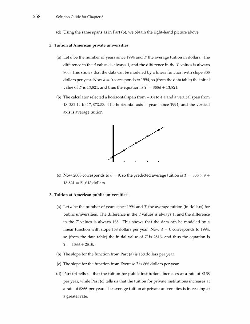
(b) The calculator selected a horizontal span from−0.4 to 4.4 and a vertical span from
13, 232.12 to 17, 873.88. The horizontal axis is years since 1994, and the vertical
axis is average tuition.
(c) Now 2003 corresponds to d = 9, so the predicted average tuition is T = 866× 9 +
13,821 = 21,615 dollars.
3. Tuition at American public universities:
(a) Let d be the number of years since 1994 and T the average tuition (in dollars) for
public universities. The difference in the d values is always 1, and the difference
in the T values is always 168. This shows that the data can be modeled by a
linear function with slope 168 dollars per year. Now d = 0 corresponds to 1994,
so (from the data table) the initial value of T is 2816, and thus the equation is
T = 168d + 2816.
(b) The slope for the function from Part (a) is 168 dollars per year.
(c) The slope for the function from Exercise 2 is 866 dollars per year.
(d) Part (b) tells us that the tuition for public institutions increases at a rate of $168
per year, while Part (c) tells us that the tuition for private institutions increases at
a rate of $866 per year. The average tuition at private universities is increasing at
a greater rate.

SECTION 3.3 Modeling Data with Linear Functions 259
(e) The percentage increase for private universities from 1997 to 1998 is866
16,419=
0.053 = 5.3%, and the percentage increase for public universities from 1997 to
1998 is1683320
= 0.051 = 5.1%. The average tuition for private universities had the
larger percentage increase from 1997 to 1998.
4. Total cost:
(a) The difference in the N values is always 50, and the difference in the C values is
always 1750. This shows that the data can be modeled by a linear function with
slope175050
= 35 dollars per widget. From the solution of Exercise 5 in Section 3.2,
we know that the variable cost is the slope, namely 35 dollars per widget. We also
know that the amount of the fixed costs is the initial value b of the function. We
find this value as follows: We have C = 35N +b, and we use the fact that C = 7900
when N = 200. This gives 7900 = 35×200+b, and thus b = 7900−35×200 = 900.
Hence the amount of the fixed costs is $900.
(b) We want to find what value of b for the function C = 35N+b will have the property
that C = 12,975 when N = 350. This gives 12,975 = 35 × 350 + b, and thus
b = 12,975 − 35 × 350 = 725. Hence the amount of the new fixed costs is $725.
Note: Here is another way to solve this part. We want to reduce the fixed costs so
as to lower the total cost at a production level of 350 from $13,150 to $12,975, that
is, by $175. Then the new fixed costs must be 900− 175 = 725 dollars.
(c) Because the variable cost is the slope m, we want to find what value of m for the
function C = mN + 900 will have the property that C = 12,975 when N = 350.
This gives 12,975 = m × 350 + 900, and thus b =12,975− 900
350= 34.5. Hence the
new variable cost is 34.50 dollars per widget. Note: Here is another way to solve
this part. We want to reduce the variable cost so as to lower the total cost at a
production level of 350 from $13,150 to $12,975, that is, by $175. This reduction
of total cost must be spread over all 350 widgets, so to accomplish this we must
reduce the variable cost by175350
= 0.50 dollar per widget. Then the new variable
cost must be 35− 0.50 = 34.50 dollars per widget.
5. Total revenue and profit:
(a) The difference in the N values is always 50, and the difference in the p values is
always −0.50. This shows that the data can be modeled by a linear function with
slope−0.50
50= −0.01 dollar per widget. Thus we have p = −0.01N +b, and we use
the fact that p = 43.00 when N = 200 to find b. This gives 43.00 = −0.01× 200 + b,
and thus b = 43.00 + 0.01× 200 = 45. Hence the model is p = −0.01N + 45.

260 Solution Guide for Chapter 3
(b) Now the total revenue is the price times the number of items, so R = pN . Using
the formula from Part (a) gives R = (−0.01N + 45)N . (This can also be written as
R = −0.01N2 + 45N .) This is not a linear function, as can be seen by examining a
table of values (or a graph) or by observing that the coefficient of N is not constant.
(c) We have P = R− C. From Part (a) of Exercise 4 we know that C has slope 35 and
initial value 900, so its formula is C = 35N + 900. Using the formula for R from
Part (b) of this exercise, we have P = (−0.01N + 45)N − (35N + 900). (This can
also be written as P = −0.01N2 + 10N − 900.) This is not a linear function, as
can be seen by examining a table of values (or a graph) or by observing that the
coefficient of N is not constant.
6. Dropping rocks on Mars:
(a) The difference in V for successive seconds is 12.16 feet per second. This tells us that
the data can be modeled with a linear equation with slope 12.16 feet per second
per second. Since the initial value of V is 0, the equation is V = 16.12t.
(b) We calculate that V (10) = 12.16 × 10 = 121.6 feet per second. This means that 10
seconds after release the velocity of the rock is 121.6 feet per second.
(c) The acceleration due to gravity on Mars is the rate of change in velocity. This is
the slope of the line in Part (a), which is 12.16 feet per second per second.
7. The Kelvin temperature scale:
(a) The change in F is always 36 degrees Fahrenheit for each 20 degree change in K
(the temperature in kelvins). This means that F is a linear function of K.
(b) The slope is calculated as
Change in F
Change in K=
3620
= 1.8.
Thus the slope is 1.8 degrees Fahrenheit per kelvin.
(c) The slope of the function is 1.8, so F = 1.8K + b for some b. To find b, we use one
point on the line; for example, when K = 200, then F = −99.67. These values give
−99.67 = 1.8× 200 + b, so b = −459.67. Thus F = 1.8K − 459.67.
(d) Now F = 98.6, and we need to find K. Thus we have to solve the equation
1.8K − 459.67 = 98.6:
1.8K − 459.67 = 98.6
1.8K = 558.27 Add 459.67 to both sides.
K = 310.15 Divide both sides by 1.8.

SECTION 3.3 Modeling Data with Linear Functions 261
Thus, body temperature on the Kelvin scale is 310.15 kelvins.
(e) Since the slope of F is 1.8, when temperature increases by one kelvin, the Fahren-
heit temperature will increase by 1.8 degrees.
If we solve F = 1.8K − 459.67 for K we get K =1
1.8F +
459.671.8
, or K = 0.56F +
255.37. So a one degree increase in Fahrenheit will increase the temperature by
0.56 kelvin.
(f) If K = 0 then F = 1.8× 0− 459.67 = −459.67 degrees Fahrenheit.
8. Further verification of Newton’s second law: Let A be acceleration, in meters per sec-
ond per second, and F the force, in newtons.
(a) Subtracting to get the differences gives
Change in A 3 3 3 3Change in F 45 45 45 45
Since the change in F is 45 for each change in A of 3, F is a linear function of A
with slope453
= 15.
(b) Since the slope is 15, we have F = 15A + b. To find b, we use the first point given,
A = 8 meters per second per second when F = 120 newtons. Thus 120 = 15×8+b,
so b = 0, and therefore the equation is simply F = 15A.
(c) The slope is the mass of 15 kilograms used in the experiment.
(d) The force resulting from an acceleration of 15 meters per second per second is
expressed in functional notation as F (15). Its value is F (15) = 15 × 15 = 225
newtons.
(e) Now F = 15A, so Force = Mass×Acceleration, as expected by Newton’s second
law of motion.
9. Market supply:
(a) By subtracting entries, we see that for each increase of 0.5 in the quantity S, there
is an increase of 1.05 in price P . Thus P is a linear function of S with slope1.050.5
=
2.1. Since the slope is 2.1, we have P = 2.1S + b. Now b can be determined using
the first data point: S = 1 when P = 1.35. Substituting, we have 1.35 = 2.1×1.0+b,
so b = −0.75, and therefore P = 2.1S − 0.75.

262 Solution Guide for Chapter 3
(b) The given table suggests a horizontal span from 0 to 3 billion bushels of wheat
and a vertical span from 0 to 5 dollars per bushel. The horizontal axis is billions of
bushels produced, and the vertical axis is price per bushel .
(c) If the price increases, then the wheat suppliers will want to produce more wheat.
This means that the market supply curve will be going up to the right, so it is
increasing.
(d) If the price P is $3.90 per bushel, then S can be determined using the formula from
Part (a): 2.1S − 0.75 = 3.90. Solving (by adding 0.75 to each side, then dividing
by 2.1) yields S = 2.21. Thus suppliers would be willing to produce 2.21 billion
bushels in a year for a price of $3.90 per bushel.
10. Market demand:
(a) By subtracting entries we find that, for each increase of 0.5 in D, there is an de-
crease of 0.30 in P (a change of −0.30). Thus P is a linear function of S with slope
Change in P
Change in D=−0.300.5
= −0.6.
Since the slope is−0.6, we have P = −0.6D+b. Now b can be determined using the
first data point: D = 1 when P = 2.05. Substituting, we have 2.05 = −0.6×1.0+b,
so b = 2.65. Therefore P = −0.6D + 2.65.
(b) Adding this graph (thick line) to that from Exercise 9 (and using the same win-
dow), we get:
SECTION 3.3 Modeling Data with Linear Functions 263
(c) As the price of wheat increases, wheat consumers will be willing to purchase less
of it. This means that the market demand curve will be doing down as it goes to
the right, so it is decreasing.
(d) The point of intersection of the two lines is calculated on the graph above and
occurs at X = 1.26 and Y = 1.89. Since, for both curves, the vertical axis is price,
the equilibrium price is $1.89 per bushel.
11. Sports car:
(a) Let t be the time since the car was at rest, in seconds, and V the velocity, in miles
per hour. The differences are in the table below:
Change in t 0.5 0.5 0.5Change in V 5.9 5.9 5.9
The ratio of change in V to change in t is always5.90.5
= 11.8, so V can be modeled
by a linear function of t with slope 11.8.
(b) The slope is 11.8 miles per hour per second. In practical terms, this means that,
after every second, the car will be going 11.8 miles per hour faster. This says that
the acceleration is constant.
(c) From Part (b), we know that V = 11.8t + b for some b. Using the first data point,
t = 2.0 and V = 27.9, we have 27.9 = 11.8 × 2.0 + b. Thus b = 4.3, and the final
formula is V = 11.8t + 4.3.
(d) According to the formula in Part (c), the initial velocity is V (0) = 4.3 miles per
hour. On the other hand, the exercise states that when t = 0, the car was at rest, so
we would expect the initial velocity to be 0, not 4.3. In practical terms, the formula
is valid only after the car has been moving a while since the acceleration is not
constant the whole time: acceleration is large initially and decreases afterwards.
(e) We need to find when V is 60. Using the formula, we have 11.8t + 4.3 = 60, so
t =60− 4.3
11.8= 4.72 seconds.
This car goes from 0 to 60 mph in 4.72 seconds.
12. High school graduates: Let d be years since 1985 and N the number of graduating high
school students, in millions.
(a) A table of differences is calculated to be:
Change in d 2 2 2Change in N −0.18 −0.18 −0.18

264 Solution Guide for Chapter 3
The ratio of change in N to change in d is always−0.18
2= −0.09, so this data can
be modeled using a linear function with slope −0.09.
(b) The slope is −0.09 million graduating high school students per year. In practical
terms, this means that each year there will be 0.09 million, or 90, 000, fewer high
school students graduating.
(c) To find the initial value, note that 1985 corresponds to d = 0. Now N = 2.83 when
d = 0, and thus the formula is N = −0.09d + 2.83.
(d) The number graduating from high school in 1994 is expressed in functional nota-
tion as N(9) since 1994 is 9 years since 1985. Its value is N(9) = −0.09×9+2.83 =
2.02 million graduating.
13. Later high school graduates: Let N be the number graduating (in millions) and t the
number of years since 1995.
(a) The difference in the t values is always 2, and the difference in the N values is
always 0.16. This shows that the data can be modeled by a linear function with
slope0.162
= 0.08 million graduating per year. The slope means that every year
the number graduating increases by 0.08 million (or 80,000).
(b) Now t = 0 corresponds to 1995, so (from the data table) the initial value of N is
2.59, and thus the equation is N = 0.08t + 2.59.
(c) The number graduating from high school in 2002 is expressed in functional nota-
tion as N(7) since 2002 is 7 years since 1995. Its value is N(7) = 0.08× 7 + 2.59 =
3.15 million graduating.
(d) Since 1994 is 1 year before 1995, we use t = −1 in the formula from Part (b). The
value is N(−1) = 0.08 × (−1) + 2.59 = 2.51 million graduating. This is much
closer to the actual number than the value of 2.02 million graduating given in Part
(d) of Exercise 12. The trend in high school graduations was a steady decline from
1985 until the early 1990s followed by a steady increase starting in 1994 or slightly
earlier.
14. Tax table: Let T be the tax and I the taxable income (both in dollars). The difference in
the I values is always 100. From I = 56,300 through I = 56,700 the difference in the
T values is always 15. This shows that the data can be modeled by a linear function
with slope15100
= 0.15 dollar per dollar over that part of the table. The model has the
form T = 0.15I + b, and we find the constant b by using the first entry in the table:
7749 = 0.15 × 56,300 + b, so b = 7749 − 0.15 × 56,300 = −696. Thus the formula from
I = 56,300 through I = 56,700 is T = 0.15I − 696.
SECTION 3.3 Modeling Data with Linear Functions 265
From I = 56,800 through I = 57,400 the difference in the T values is always 25. This
shows that the data can be modeled by a linear function with slope25100
= 0.25 dollar
per dollar over that part of the table. The model has the form T = 0.25I + b, and
we find the constant b by using the entry I = 56,800, T = 7826 in the table: 7826 =
0.25×56,800+b, so b = 7826−0.25×56,800 = −6374. Thus the formula from I = 56,800
through I = 57,400 is T = 0.25I − 6374.
For each part of the table the slope gives the marginal tax rate for that part—that is, it
gives the extra tax owed (in dollars) when the taxable income increases by $1. Thus, for
a taxable income between $56,300 and $56,700, extra taxable income is taxed at a rate of
15 cents on the dollar. For a taxable income between $56,800 and $57,400, extra taxable
income is taxed at a rate of 25 cents on the dollar.
15. Sound speed in oceans:
(a) Here is a table of differences:
Change in S 0.6 0.6 0.6 0.6Change in c 0.72 0.72 0.82 0.62
From this table it is clear that the fourth entry for speed (at the salinity of S = 36.8)
is in error—it is too high by 0.1. When S = 36.8, c should be 1517.62 − 0.1 =
1517.52. With this choice, all entries are consistent with a linear model.
(b) The linear model has slope
Change in c
Change in S=
0.720.6
= 1.2 meters per second per parts per thousand.
The slope means that, at the given depth and temperature, for an increase in salin-
ity of 1 part per thousand the speed of sound increases by 1.2 meters per second.
(c) We use the slope, 1.2, and the last entry in the table. Because
Change in c = Slope × Change in S,
we have
c(39)− c(37.4) = 1.2× (39− 37.4),
and thus
c(39) = c(37.4) + 1.2× (39− 37.4) = 1518.24 + 1.2× (39− 37.4) = 1520.16.
This means that the speed of sound is 1520.16 meters per second when the salinity
is 39 parts per thousand. Note: The value of c(39) can also be found by first using
the slope and an entry in the table to find the formula for c, namely c = 1.2S +
1473.36.

266 Solution Guide for Chapter 3
16. Focal length:
(a) The difference in the Fe values is always 0.2, and the difference in the Fo values
is always 16. This shows that the data can be modeled by a linear function with
slope160.2
= 80 centimeters per centimeter. The model has the form Fo = 80Fe + b,
and we find the constant b by using the first entry in the table: 24 = 80 × 0.3 + b,
so b = 24− 80× 0.3 = 0. Thus the model is Fo = 80Fe.
(b) Because Fo is proportional to Fe with constant of proportionality M , the formula
is Fo = MFe.
(c) To solve for M in the equation Fo = MFe, we divide both sides by Fe and obtain
M =Fo
Fe.
(d) To make the fraction in the formula M =Fo
Felarge, we should make the numerator
large and the denominator relatively small. Thus the objective lens should have a
large focal length and the eyepiece a relatively small focal length.
17. Measuring the circumference of the Earth: Because the rate of travel is 100 stades per
day, a trip requiring 50 days is 100 × 50 = 5000 stades long. This is estimated to be150
of the Earth’s circumference, so Eratosthenes’ measure of the circumference of the
Earth is 5000× 50 = 250,000 stades. This is 250,000× 0.104 = 26,000 miles.
18. A research project on tax tables: This is a relatively brief solution.
(a) Let T be the tax and I the taxable income (both in dollars). The difference in the I
values is always 100. From I = 57,300 through I = 58,000 the difference in the T
values is always 15. This shows that the data can be modeled by a linear function
with slope15100
= 0.15 dollar per dollar over that part of the table. The model has
the form T = 0.15I + b, and we find the constant b by using the first entry in the
table: 7884 = 0.15 × 57,300 + b, so b = 7884 − 0.15 × 57,300 = −711. Thus the
formula from I = 57,300 through I = 58,000 is T = 0.15I − 711.
From I = 58,100 through I = 58,400 the difference in the T values is always 25.
This shows that the data can be modeled by a linear function with slope25100
=
0.25 dollar per dollar over that part of the table. The model has the form T =
0.25I + b, and we find the constant b by using the entry I = 58,100, T = 8006 in
the table: 8006 = 0.25× 58,100 + b, so b = 8006− 0.25× 58,100 = −6519. Thus the
formula from I = 58,100 through I = 58,400 is T = 0.25I − 6519.
(b) For both tables the first part is modeled by a linear function with slope 0.15 dollar
per dollar, and the second part is modeled by a linear function with slope 0.25

SECTION 3.4 Linear Regression 267
dollar per dollar. For the first table the transition occurs between taxable incomes
of $56,700 and $56,800; for the second, the transition occurs between taxable in-
comes of $58,000 and $58,100. In the later year the transition occurs at higher
incomes. The transition level is important because the marginal tax rate increases
significantly at this point.
(c) By law the transition level is increased from one year to the next in accordance
with the inflation rate. This is an attempt to prevent bracket creep, when taxpay-
ers are bumped into a higher tax bracket by the inflation of incomes even when
incomes adjusted for inflation have not risen.
3.4 LINEAR REGRESSION
E-1 Fitting lines: Answers will vary according to the choice of the estimate line for the fed-
eral education expenditures. For example, I might choose a line E with the same slope,
1.275, as Est, but which passes through the third data point (2, 30.4). Such a line has
equation E − 30.4 = 1.275(x − 2), so E = 1.275x + 27.85. The table below shows the
calculations to find the squares of the errors for E.
Year Data Estimate Error of estimate Square of error of estimatex y E y − E (y − E)2
0 27.0 27.850 −0.850 0.72251 29.0 29.125 −0.125 0.01562 30.4 30.400 0 03 30.9 31.675 −0.775 0.60064 32.1 32.950 −0.850 0.7225
The sum of the squares of the errors is the sum of the last column, which is 2.0612.
Clearly this is not better fit than Est.
E-2 Calculating regression lines: In each case, we construct a table to compute Sx2, the sum
of the x-deviations, and Sxy, the sum of the products of the deviations.
(a) The averages are x =0 + 2 + 4 + 6
4= 3 and y =
1 + 6 + 13 + 204
= 10.
x-deviation y-deviation x-deviation squared Product of deviationsx y x− 3 y − 10 (x− 3)2 (x− 3)× (y − 10)0 1 −3 −9 9 272 6 −1 −4 1 44 13 1 3 1 36 20 3 10 9 30

268 Solution Guide for Chapter 3
Thus Sx2 = 9 + 1 + 1 + 9 = 20 and Sxy = 27 + 4 + 3 + 30 = 64, and therefore the
regression line is
Reg = y +Sxy
Sx2(x− x) = 10 +
6420
(x− 3) =6420
x− 3× 6420
+ 10 = 3.2x + 0.4.
(b) The averages are x =0 + 3 + 5 + 9
4= 4.25 and y =
−1 + 6 + 8 + 164
= 7.25.
x-deviation y-deviation x-deviation squared Product of deviationsx y x− 4.25 y − 7.25 (x− 4.25)2 (x− 4.25)× (y − 7.25)0 −1 −4.25 −8.25 18.0625 35.06253 6 −1.25 −1.25 1.5625 1.56255 8 0.75 0.75 0.5625 0.56259 16 4.75 8.75 22.5625 41.5625
Thus Sx2 = 42.75 and Sxy = 78.75, and therefore the regression line is
Reg = y+Sxy
Sx2(x−x) = 7.25+
78.7542.75
(x−4.25) =78.7542.75
x−4.2578.7542.75
+7.25 = 1.84x−0.58.
(c) The averages are x =1 + 2 + 6 + 7
4= 4 and y =
6 + 9 + 23 + 264
= 16.
x-deviation y-deviation x-deviation squared Product of deviationsx y x− 4 y − 16 (x− 4)2 (x− 4)× (y − 16)1 6 −3 −10 9 302 9 −2 −7 4 146 23 2 7 4 147 26 3 10 9 30
Thus Sx2 = 26 and Sxy = 88, and therefore the regression line is
Reg = y +Sxy
Sx2(x− x) = 16 +
8826
(x− 4) =8826
x− 4× 8826
+ 16 = 3.38x + 2.46.
E-3 Calculating the error: For each data set in Exercise S-2, we form a table that shows the
calculations yielding the sum-of-squares error for the regression line Reg.
(a) Here we use Reg = 3.2x + 0.4.
Regression Error of regression Square of error of regressionx y Reg y − Reg (y − Reg)2
0 1 0.4 0.6 0.362 6 6.8 −0.8 0.644 13 13.2 −0.2 0.046 20 19.6 0.4 0.16
Thus the sum-of-squares error for the regression line is 0.36+0.64+0.04+0.16 = 1.2.

SECTION 3.4 Linear Regression 269
(b) Here we use Reg = 1.84x− 0.57.
Regression Error of regression Square of error of regressionx y Reg y − Reg (y − Reg)2
0 −1 −0.58 −0.42 0.17643 6 4.95 1.05 1.10255 8 8.63 −0.63 0.39699 16 15.99 0.01 0.0001
Thus the sum-of-squares error for the regression line is 0.1764 + 1.1025 + 0.3969 +
0.0001 = 1.6759, or about 1.68.
(c) Here we use Reg = 3.38x + 2.46.
Regression Error of regression Square of error of regressionx y Reg y − Reg (y − Reg)2
1 6 5.84 0.16 0.02562 9 9.22 −0.22 0.04846 23 22.74 0.26 0.06767 26 26.12 −0.12 0.0144
Thus the sum-of-squares error for the regression line is 0.0256 + 0.0484 + 0.0676 +
0.0144 = 0.156.
E-4 Military expenditures:
(a) To calculate the regression line L for military expenditures M as a function of t,
we use a table to show the calculations. Using the data from Example 3.9, we
first calculate the averages. The averages are t =0 + 1 + 2 + 3 + 4
5= 2 and M =
252.7 + 263.3 + 282.0 + 290.4 + 303.65
= 278.4.
t-deviation M -deviation t-deviation squared Product of deviationst M t− 2 M − 278.4 (t− 2)2 (t− 2)× (M − 278.4)0 252.7 −2 −25.7 4 51.41 263.3 −1 −15.1 1 15.12 282.0 0 3.6 0 03 290.4 1 12 1 124 303.6 2 25.2 4 50.4
Thus St2 = 10 and StM = 128.9, and therefore the regression line is
L = M+StM
St2(t−t) = 278.4+
128.910
(t−2) = 12.89t+278.4−2×12.89 = 12.89t+252.62.
(b) To evaluate the formula for L from Part (a) at t = t = 2, we calculate L(2) =
12.89 × 2 + 252.62 = 278.4, which exactly equals M . (In general, it is always true
that Reg(x) = y.)

270 Solution Guide for Chapter 3
E-5 The meaning of errors:
(a) If the sum of the squares of the errors of an estimate is 0, then, since each square is
non-negative, this would mean that each error is 0. In this case, then, the line would
fit the data points exactly.
(b) For each data set and regression line found in Exercise E-2, the errors are found as
the fourth column in the tables in Exercise E-3. The sum of each fourth column is
zero, allowing for rounding. (In general, it is always true that the sum of the errors
of the regression line is 0.)
E-6 Correlation coefficient:
(a) Entering the data in a calculator, we have found the regression line and correlation
coefficient as shown in the figure below on the left. The regression line is y = 2x+1
and the correlation coefficient is r = 1, indicating an exact fit. The figure on the
right below shows a plot of the data together with a graph of the regression line.
(b) Entering the data in a calculator, we have found the regression line and correlation
coefficient as shown in the figure below on the left. The regression line is y = 2x+1.4
and the correlation coefficient is r = 0.99, indicating a very close, but not exact, fit.
The figure on the right below shows a plot of the data together with a graph of the
regression line.

SECTION 3.4 Linear Regression 271
(c) Entering the data in a calculator, we have found the regression line and correlation
coefficient as shown in the figure below on the left. The regression line is y = 2x+2.4
and the correlation coefficient is r = 0.90, indicating an approximate fit. The figure
on the right below shows a plot of the data together with a graph of the regression
line.
S-1. Slope of regression line: If the slope of the regression line is positive, then the line is
increasing, so we expect overall the data values to be increasing.
S-2. Meaning of slope of regression line: If the slope of the regression line for money spent
on education as a function of the year is $2300 per year, then this means that as a trend
each year the money spent on education increases by about $2300.
S-3. Meaning of slope of regression line: If the slope of the regression line for federal agri-
cultural spending is larger than the slope of the regression line for federal spending
on research and development, then this means that federal spending on agriculture is
increasing faster than federal spending on research and development.
S-4. Meaning of slope of regression line: If the slope of the regression line for speed run-
ning as a function of length is 2.03 miles per hour per inch, then this means that each
additional inch in length adds about 2.03 miles per hour to the running speed.
S-5. Plotting data and regression lines: The figure below on the left is a plot of the data. The
regression line is y = −0.26x + 2.54. The figure on the right below is the plot of the data
with the graph of the regression line added.

272 Solution Guide for Chapter 3
S-6. Plotting data and regression lines: The figure below on the left is a plot of the data. The
regression line is y = −0.32x + 3.14. The figure on the right below is the plot of the data
with the graph of the regression line added.
S-7. Plotting data and regression lines: The figure below on the left is a plot of the data. The
regression line is y = 1.05x + 2.06. The figure on the right below is the plot of the data
with the graph of the regression line added.
S-8. Plotting data and regression lines: The figure below on the left is a plot of the data. The
regression line is y = 0.21x + 6.93. The figure on the right below is the plot of the data
with the graph of the regression line added.

SECTION 3.4 Linear Regression 273
S-9. Plotting data and regression lines: The figure below on the left is a plot of the data. The
regression line is y = −0.32x− 1.59. The figure on the right below is the plot of the data
with the graph of the regression line added.
S-10. Plotting data and regression lines: The figure below on the left is a plot of the data. The
regression line is y = 3.09x + 3.92. The figure on the right below is the plot of the data
with the graph of the regression line added.
S-11. Meaning of slope of regression line: If the slope of the regression line for average life
expectancy of children as a function of year of birth is 0.16, then for each increase of 1 in
the year of birth the life expectancy increases by 0.16 year, or about 2 months.
S-12. Plotting data and regression lines: The figure below on the left is a plot of the data. The
regression line is y = −4.3x + 5.37. The figure on the right below is the plot of the data
with the graph of the regression line added.

274 Solution Guide for Chapter 3
1. Is a linear model appropriate?
(a) The plotted points are shown below.
The plot of the data appears to be fit better by a curve rather than by a straight
line.
(b) We take the variable to be years since 1996. The plotted points are shown below.
It looks like the points almost fall on a straight line. It appears reasonable to ap-
proximate this data with a straight line.
2. College enrollment: Let t be the number of years since 1996 and E the enrollment in
public colleges, in millions.
(a) From the left-hand figure below, the equation of the regression line is E = 0.13t +
11.1. Adding this line to the graph from Exercise 1 gives the right-hand picture
below. The horizontal axis is years since 1996, and the vertical axis is enrollment
in American public colleges.

SECTION 3.4 Linear Regression 275
(b) The slope of the regression line is 0.13, and this means that every year the enroll-
ments in American public colleges increased by about 0.13 million.
(c) The enrollment in American public colleges in 2002 is E(6) in functional notation,
since t = 6 corresponds to the year 2002. Using the regression line, we calculate
E(6) = 0.13× 6 + 11.1 = 11.88, or about 11.9, million.
(d) The year 1993 is three years before 1996, so t = −3. The regression estimate for
1993 is E(−3) = 0.13 × (−3) + 11.1 = 10.71 million, which is considerably below
the actual enrollment of 11.2 million, so it appears that the trend in the late 1990s
was not valid as early as 1993.
3. Tourism: Let t be the number of years since 1994 and T the number of tourists, in
millions.
(a) A plot of the data points is shown below.
(b) From the left-hand figure below, the equation of the regression line is T = 1.92t +
18.61. Adding this line to the plot above gives the right-hand figure below. The
horizontal axis is years since 1994, and the vertical axis is millions of tourists.
(c) The slope of the regression line is 1.92, and this means that every year the number
of tourists who visited the United States from overseas increases by about 1.92
million.
(d) The number of tourists who visited the United States in 2001 is T (7) in functional
notation, since t = 7 corresponds to seven years after 1994, that is, the year 2001.
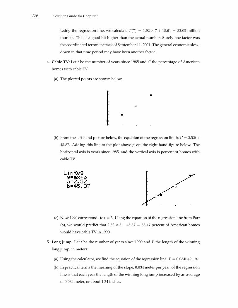
276 Solution Guide for Chapter 3
Using the regression line, we calculate T (7) = 1.92 × 7 + 18.61 = 32.05 million
tourists. This is a good bit higher than the actual number. Surely one factor was
the coordinated terrorist attack of September 11, 2001. The general economic slow-
down in that time period may have been another factor.
4. Cable TV: Let t be the number of years since 1985 and C the percentage of American
homes with cable TV.
(a) The plotted points are shown below.
(b) From the left-hand picture below, the equation of the regression line is C = 2.52t+
45.87. Adding this line to the plot above gives the right-hand figure below. The
horizontal axis is years since 1985, and the vertical axis is percent of homes with
cable TV.
(c) Now 1990 corresponds to t = 5. Using the equation of the regression line from Part
(b), we would predict that 2.52 × 5 + 45.87 = 58.47 percent of American homes
would have cable TV in 1990.
5. Long jump: Let t be the number of years since 1900 and L the length of the winning
long jump, in meters.
(a) Using the calculator, we find the equation of the regression line: L = 0.034t+7.197.
(b) In practical terms the meaning of the slope, 0.034 meter per year, of the regression
line is that each year the length of the winning long jump increased by an average
of 0.034 meter, or about 1.34 inches.

SECTION 3.4 Linear Regression 277
(c) The figure below shows a plot the data points together with a graph of the regres-
sion line.
(d) The regression line formula has positive slope and so increases without bound.
Surely there is some length that cannot be attained by a long jump, and therefore
the regression line is not necessarily a good model of the winning length over a
long period of time.
(e) The regression line model gives the value L(20) = 0.034 × 20 + 7.197 = 7.877, or
about 7.88, meters, which is over two feet longer than the length of the winning
long jump in the 1920 Olympic Games. This result is consistent with our answer
to Part (d) above.
6. Driving:
(a) The equation of the regression line expressing S as a linear function of t is S =
0.23t + 55.
(b) In practical terms the meaning of the slope, 0.23 mile per hour per second, of the
regression line is that for each additional second, our speed increases by 0.23 mile
per hour.
(c) Based on the regression line model, our speed will reach 70 miles per hour when
70 = 0.23t + 55. Solving for t, we have 0.23t = 70− 55 = 15, and so we will reach
70 miles per hour when t =15
0.23= 65.22, or about 65, seconds after starting our
observations.

278 Solution Guide for Chapter 3
(d) The figure below shows a plot the data points together with a graph of the regres-
sion line.
(e) Looking at the plot in Part (d), we see that the middle three data points are above
the line and then the last one is below the line, so it seems that for later times the
data points may well stray further below the line. In fact, the plot indicates that
the speed is increasing at a decreasing rate. Thus our prediction in Part (c) is likely
to give a time earlier than the actual time when our speed reaches 70 miles per
hour.
7. The effect of sampling error on linear regression:
(a) The plotted points are shown below.
(b) From the left-hand figure below, the equation of the regression line is D = 0.88t +
51.98. In practical terms, the slope of 0.88 foot per hour means that the flood waters
are rising by 0.88 foot each hour.

SECTION 3.4 Linear Regression 279
(c) Adding the regression line to the plot gives the right-hand figure below. The hor-
izontal axis is time since flooding began, and the vertical axis is depth.
(d) Adding D = 0.8t + 52 (thick line) gives the following graph.
So the data does give a close approximation of the depth function, since the two
lines are very close. The regression model shows a water level which is a bit too
high.
(e) From the depth function D = 0.8t + 52, the actual depth of the water after 3 hours
is 0.8× 3 + 52 = 54.4 feet.
(f) The regression line equation predicts the depth after 3 hours to be 0.88×3+51.98 =
54.62, or about 54.6, feet.

280 Solution Guide for Chapter 3
8. Gross national product: Let t be the number of years since 1998 and G the gross na-
tional product, in trillions of dollars.
(a) From the left-hand figure below, the equation of the regression line is G = 0.41t +
8.87. In practical terms, the slope of the line being 0.41 tells us that each year
the gross national product increases by 0.41 trillion dollars, or about 410 billion
dollars.
(b) Plotting both the data points and the regression line gives the right-hand figure
below. The horizontal axis is years since 1998, and the vertical axis is gross national
product, in trillions of dollars.
(c) Now 2006 corresponds to t = 8. The equation of the regression line gives a predic-
tion for the gross national product of G = 0.41 × 8 + 8.87 = 12.15 trillion dollars.
The economist predicted 13 trillion, which is higher, so our information from Part
(a) does not support that conclusion. According to the regression line prediction,
the gross national product reaches 13 trillion when 0.41t + 8.87 = 13. Solving for t
gives that t = 10.07, which roughly corresponds to 2008. So the GNP should about
reach 13 trillion dollars by 2008.
9. Japanese auto sales in the U.S.: Let t be the number of years since 1992 and J the total
U.S. sales of Japanese automobiles, in millions.
(a) The data points are plotted below.

SECTION 3.4 Linear Regression 281
It may be reasonable to model this with a linear function, but there is room for
argument here. There is enough deviation from a straight line to cast some doubt
on whether the use of a linear model would be appropriate. The collection of
additional data would be wise.
(b) From the left-hand figure below, the equation of the regression line is J = −0.044t+
2.46. The slope is -0.044, which means that each year the total US sales of Japanese
cars decreases by 0.044 million cars, or about 44,000 cars.
(c) The regression line has been added in the right-hand figure below. The horizontal
axis is years since 1992, and the vertical axis is millions of auto sales.
To the eyes of the authors, this picture makes the use of the regression line appear
more appropriate than does the appearance of the plotted data alone. Gathering
more data still seems advisable.
(d) Now 1997 corresponds to t = 5, and 1998 corresponds to t = 6. From the equation
of the regression line, we expect J = −0.044 × 5 + 2.46 = 2.24 million cars to be
sold in 1997 and J = −0.044 × 6 + 2.46 = 2.196, or about 2.20, million cars to
be sold in 1998. The regression line estimates are higher than the Department of
Commerce’s figures in both cases.
10. Running speed versus length:
(a) The table indicates that as the length of the animal increases so does the maximum
speed. So it is generally true that larger animals run faster.
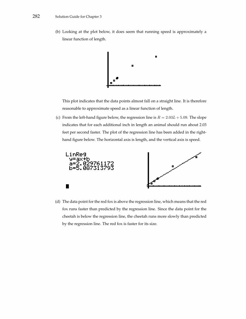
282 Solution Guide for Chapter 3
(b) Looking at the plot below, it does seem that running speed is approximately a
linear function of length.
This plot indicates that the data points almost fall on a straight line. It is therefore
reasonable to approximate speed as a linear function of length.
(c) From the left-hand figure below, the regression line is R = 2.03L + 5.09. The slope
indicates that for each additional inch in length an animal should run about 2.03
feet per second faster. The plot of the regression line has been added in the right-
hand figure below. The horizontal axis is length, and the vertical axis is speed.
(d) The data point for the red fox is above the regression line, which means that the red
fox runs faster than predicted by the regression line. Since the data point for the
cheetah is below the regression line, the cheetah runs more slowly than predicted
by the regression line. The red fox is faster for its size.

SECTION 3.4 Linear Regression 283
11. Antimasonic voting: Using the notation of M as the percentage antimasonic voting
and C as the number of church buildings, the statement to be analyzed is “M depends
directly on C,” that is, M is a linear function of C. The data plot is shown below.
From the left-hand figure below, the equation for the regression line is M = 5.89C +
45.55; moreover, plotting that equation with the data points gives the right-hand figure.
The horizontal axis is number of churches and the vertical axis is percent antimasonic
voting.
The figure shows that the regression line fits the data well. So the data does support
the premise of the stated direct dependence.
12. Running ants: Let T be the ambient temperature, in degrees Celsius, and S the ants’
speed, in centimeters per second.
(a) From the figure below, the equation of the regression line for S is S = 0.21T −2.73.

284 Solution Guide for Chapter 3
(b) In practical terms, the slope of 0.21 means that for each increase in temperature of
one degree Celsius, the ants run 0.21 centimeter per second faster.
(c) Using functional notation, we express the speed at which the ants run when the
ambient temperature is 29 degrees Centigrade by S(29). According to the regres-
sion estimate, S(29) = 0.21× 29− 2.73 = 3.36 centimeters per second.
(d) If the ants are running at 2.5 centimeters per second, then S = 2.5. Using the
equation from Part (a), we have 0.21T − 2.73 = 2.5. Solving this yields T = 24.9
degrees Celsius.
13. Expansion of steam:
(a) The linear regression model of volume V as a function of T is V = 12.57T +
7501.00.
(b) If one fire is 100 degrees hotter than another, then T increases by 100, so V in-
creases by 12.57×100 = 1257; that is, the volume of steam produced by 50 gallons
of water in the hotter fire is 1257 cubic feet more.
(c) The volume V (420) = 12.57× 420 + 7501 = 12,780.4 cubic feet. In practical terms
this answer means that 50 gallons of water applied to a fire of 420 degrees Fahren-
heit will produce about 12,780 cubic feet of steam.
(d) If 50 gallons of water expanded to 14,200 cubic feet of steam, then V = 14,200, and
so 14,200 = 12.57T + 7501. Solving for T , we find that 12.57T = 14,200 − 7501 =
6699. Thus T =669912.57
= 532.94, and therefore the temperature of the fire was
532.94 degrees Fahrenheit.
14. Technological maturity versus use maturity: Let T be technological maturity and let
U be use maturity, each as percents.
(a) Using regression, we find a linear regression model for use maturity as a function
of technological maturity: U = 1.14T − 12.46.
(b) In practical terms the meaning of the slope, 1.14, of the regression line is that a 1
percentage point increase in technological maturity will result in a 1.14 percentage
point increase in use maturity. More plainly, an increase of 1 percentage point
toward technological perfection of a process means that the process will be used
an additional 1.14 percentage point of total reasonable use.
(c) In functional notation, the use maturity of a process that has a technological matu-
rity of 89%, is U(89). The value of U(89), according to the regression model from
Part (a), is 1.14× 89− 12.46 = 89, so the use maturity is also 89%.

SECTION 3.4 Linear Regression 285
(d) If a process has a technological maturity of T = 73%, then the linear model would
predict a use maturity of U(73) = 1.14×73−12.46 = 70.76%. Since solvent extrac-
tion has a use maturity of only 61%, it is being used less than would be expected.
This information could affect a possible decision to get into the business of sell-
ing solvent equipment to industry either as a positive effect (solvent extraction
is under-utilized, so there is larger potential market) or a negative effect (solvent
extraction is under-utilized, so perhaps it is more difficult to use than previously
anticipated).
(e) To construct a linear model for technological maturity as a function of use matu-
rity, we take the equation U = 1.14T − 12.46 and solve for T :
U = 1.14T − 12.46
U + 12.46 = 1.14T
T =U + 12.46
1.14.
This can also be written as T = 0.88U+10.93. Alternatively, we could use linear re-
gression directly by interchanging the data columns on our calculator. Regression
gives T = 0.87U + 11.54.
15. Whole crop weight versus rice weight:
(a) Using regression, we find a linear model B = 0.29W + 0.01 for B as a function of
W .
(b) Comparing the predicted rice weight from the linear model of Part (a) with the
data, we see that the third sample, with W = 13.7 and B = 3.7 has a significantly
lower rice weight than expected from the whole crop weight. This can also be seen
by plotting the data with the regression line.
W Data B Data Predicted B = 0.29W + 0.016 1.8 1.75
11.1 3.2 3.2313.7 3.7 3.9814.9 4.3 4.3317.6 5.2 5.11
(c) An increase in whole crop weight W of one ton per hectare is expected to produce
an increase in rice weight B of 0.29 ton per hectare.
16. Rice production in Asia:
(a) An approximate linear model for Y as a function of t can be obtained using regres-
sion: Y = 0.05t + 1.47.

286 Solution Guide for Chapter 3
(b) The slope, 0.05, of the linear model from Part (a) tells us that each year there is an
increase in average rice yield of 0.05 ton per hectare.
(c) According to our model, Y (30) = 0.05 × 30 + 1.47 = 2.97. In practical terms this
means that in 1980 the average rice yield was 2.97 tons per hectare.
(d) The model estimates that for 1990 the rice yield would be Y (40) = 0.05×40+1.47 =
3.47 tons per hectare.
(e) Rice production for 2005 is estimated to be Y (55) = 0.05 × 55 + 1.47 = 4.22 tons
per hectare, which is less than the actual rice requirements of 4.92 tons per hectare.
17. Energy cost of running:
(a) From the figure below, the equation of regression line for E in terms of v is E =
0.34v + 0.37.
(b) The cost of transport is defined to be the slope of the regression line in Part (a), so
the cost of transport is 0.34, in units of (unit of E) per (unit of v), which is milliliter
of oxygen per gram per hour per kilometer per hour.
(c) If a rhea weighs 22,000 grams, then W = 22, 000. The formula for C gives C =
8.5 × 22, 000−0.40 = 0.16. The figure found for the cost of transport in Part (b) is
much higher than what the general formula would predict. Based on this, the rhea
is a much less efficient runner that a typical animal of its size.
(d) If the rhea is at rest, then v = 0. Using v = 0 in the regression equation from Part
(a) gives E = 0.37 as an estimate for the oxygen consumption for a rhea at rest.
Surely this estimate is higher than the actual oxygen consumption level at rest,
since we expect animals to be very inefficient in running at very low speeds.
18. Laboratory experiment: Answers will vary. Please refer to the website for details and
instructions.
19. Laboratory experiment: Answers will vary. Please refer to the website for details and
instructions.

SECTION 3.5 Systems of Equations 287
20. Laboratory experiment: Answers will vary. Please refer to the website for details and
instructions.
21. Research project: Answers will vary. Please refer to the website for details and instruc-
tions.
3.5 SYSTEMS OF EQUATIONS
E-1. Using elimination to solve systems of equations:
(a) We start with
x + y = 5
x− y = 1.
If we add the equations together, since the y’s cancel out, keep the first equation
and replace the second, we have
x + y = 5
2x = 6.
Thus x = 3. Plugging x = 3 into the first equation, we have 3 + y = 5 and so y = 2.
(b) We start with
2x− y = 0
3x + 2y = 14.
If we multiply the first equation by 3 and the second equation by 2, then we have
6x− 3y = 0
6x + 4y = 28.
Subtracting the first from the second and, as before, keeping the first, but replacing
the second by the difference, we have
6x− 3y = 0
7y = 28.
Thus y = 4. Plugging y = 4 into the first equation, we have 6x − 3 × 4 = 0, so
6x = 12, and therefore x = 2.

288 Solution Guide for Chapter 3
(c) We start with
3x + 2y = 6
4x− 3y = 8.
If we multiply the first equation by 4 and the second equation by 3, then we have
12x + 8y = 24
12x− 9y = 24.
Subtracting first from the second and, as before, keeping the first, but replacing the
second by the difference, we have
12x + 8y = 24
−17y = 0.
Thus y = 0. Plugging y = 0 into the first equation, we have 12x = 24, and so x = 2.
E-2. Solving larger systems of equations:
(a) We start with
x + y + z = 3
2x− y + 2z = 3
3x + 3y − z = 9.
Replacing the second equation with itself minus twice the first equation and re-
placing the third equation with itself minus three times the first equation, we have
x + y + z = 3
−3y = −3
−4z = 0.
Thus z = 0 and y = 1. Plugging these into the first equation, we get x + 1 + 0 = 3,
so x = 2.
(b) We start with
x− y − z = −2
3x− y + 3z = 8
2x + 2y + z = 6.

SECTION 3.5 Systems of Equations 289
Replacing the second equation with itself minus three times the first equation and
replacing the third equation with itself minus twice the first equation, we have
x− y − z = −2
2y + 6z = 14
4y + 3z = 10.
Now replace the third equation with itself minus twice the second equation:
x− y − z = −2
2y + 6z = 14
−9z = −18.
Thus z = 2 and, plugging this into the second equation, 2y + 6× 2 = 14, so 2y = 2
and therefore y = 1. Finally, plugging the values for y and z into the first equation,
we have x− 1− 2 = −2, so x = 1.
(c) We start with
x + y + z + w = 8
2x− y + z − w = −1
3x + y − z + 2w = 9
x + 2y + 2z + w = 12.
Replacing the second equation with itself minus twice the first equation, replacing
the third equation with itself minus three times the first equation, and replacing
the fourth equation with itself minus the first equation, we have
x + y + z + w = 8
−3y − z − 3w = −17
−2y − 4z − w = −15
y + z = 4.
To help cancel the coefficients of y, multiply the second equation by 2, the third
equation by 3, and the fourth equation by 6:
x + y + z + w = 8
−6y − 2z − 6w = −34
−6y − 12z − 3w = −45
6y + 6z = 24.
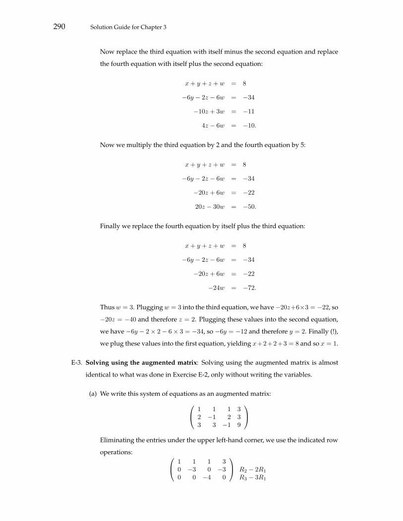
290 Solution Guide for Chapter 3
Now replace the third equation with itself minus the second equation and replace
the fourth equation with itself plus the second equation:
x + y + z + w = 8
−6y − 2z − 6w = −34
−10z + 3w = −11
4z − 6w = −10.
Now we multiply the third equation by 2 and the fourth equation by 5:
x + y + z + w = 8
−6y − 2z − 6w = −34
−20z + 6w = −22
20z − 30w = −50.
Finally we replace the fourth equation by itself plus the third equation:
x + y + z + w = 8
−6y − 2z − 6w = −34
−20z + 6w = −22
−24w = −72.
Thus w = 3. Plugging w = 3 into the third equation, we have−20z+6×3 = −22, so
−20z = −40 and therefore z = 2. Plugging these values into the second equation,
we have −6y − 2× 2− 6× 3 = −34, so −6y = −12 and therefore y = 2. Finally (!),
we plug these values into the first equation, yielding x+2+2+3 = 8 and so x = 1.
E-3. Solving using the augmented matrix: Solving using the augmented matrix is almost
identical to what was done in Exercise E-2, only without writing the variables.
(a) We write this system of equations as an augmented matrix: 1 1 1 32 −1 2 33 3 −1 9
Eliminating the entries under the upper left-hand corner, we use the indicated row
operations: 1 1 1 30 −3 0 −30 0 −4 0
R2 − 2R1
R3 − 3R1

SECTION 3.5 Systems of Equations 291
This matrix corresponds to the system of equations
x + y + z = 3
−3y = −3
−4z = 0,
which can be solved exactly as in Exercise E-2.
(b) We write this system of equations as an augmented matrix: 1 −1 −1 −23 −1 3 82 2 1 6
Eliminating the entries under the upper left-hand corner, we use the indicated row
operations: 1 −1 −1 −20 2 6 140 4 3 10
R2 − 3R1
R3 − 2R1
Eliminating the entry under the 2 in the second row: 1 −1 −1 −20 2 6 140 0 −9 −18
R3 − 2R2
This matrix corresponds to the system of equations
x− y − z = −2
2y + 6z = 14
−9z = −18,
which can be solved exactly as in Exercise E-2.
(c) We write this system of equations as an augmented matrix:1 1 1 1 82 −1 1 −1 −13 1 −1 2 91 2 2 1 12
Eliminating the entries under the upper left-hand corner, we use the indicated row
operations: 1 1 1 1 80 −3 −1 −3 −170 −2 −4 −1 −150 1 1 0 4
R2 − 2R1
R3 − 3R1
R4 −R1
We multiply to simplify the elimination in the second column:1 1 1 1 80 −6 −2 −6 −340 −6 −12 −3 −450 6 6 0 24
2R2
3R3
6R4

292 Solution Guide for Chapter 3
And then we eliminate below the −6 in the second row:1 1 1 1 80 −6 −2 −6 −340 0 −10 3 −110 0 4 −6 −10
R3 −R2
R4 + R2
Finally we eliminate below the −10 in the third row:1 1 1 1 80 −6 −2 −6 −340 0 −10 3 −110 0 0 −24 −72
5R4 + 2R3
This matrix corresponds to the system of equations
x + y + z + w = 8
−6y − 2z − 6w = −34
−20z + 6w = −22
−24w = −72,
which can be solved exactly as in Exercise E-2.
E-4. Systems of equations with many solutions:
(a) We start with
x + y + z = 6
2x + y − z = 1
4x + 3y + z = 13,
and form its augmented matrix: 1 1 1 62 1 −1 14 3 1 13
We begin to solve by eliminating the terms below the upper left-hand corner: 1 1 1 6
0 −1 −3 −110 −1 −3 −11
R2 − 2R1
R3 − 4R1
Eliminating the term below the −1 in the second row, we multiply R2 by −1 and
then we add R2 to R3 to get 1 1 1 60 1 3 110 0 0 0
.
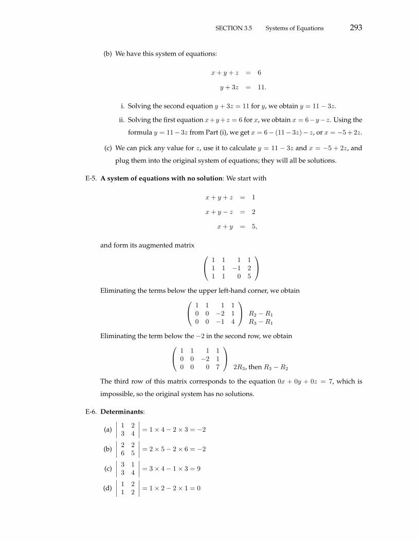
SECTION 3.5 Systems of Equations 293
(b) We have this system of equations:
x + y + z = 6
y + 3z = 11.
i. Solving the second equation y + 3z = 11 for y, we obtain y = 11− 3z.
ii. Solving the first equation x+y+z = 6 for x, we obtain x = 6−y−z. Using the
formula y = 11− 3z from Part (i), we get x = 6− (11− 3z)− z, or x = −5 + 2z.
(c) We can pick any value for z, use it to calculate y = 11 − 3z and x = −5 + 2z, and
plug them into the original system of equations; they will all be solutions.
E-5. A system of equations with no solution: We start with
x + y + z = 1
x + y − z = 2
x + y = 5,
and form its augmented matrix 1 1 1 11 1 −1 21 1 0 5
Eliminating the terms below the upper left-hand corner, we obtain 1 1 1 1
0 0 −2 10 0 −1 4
R2 −R1
R3 −R1
Eliminating the term below the −2 in the second row, we obtain 1 1 1 10 0 −2 10 0 0 7
2R3, then R3 −R2
The third row of this matrix corresponds to the equation 0x + 0y + 0z = 7, which is
impossible, so the original system has no solutions.
E-6. Determinants:
(a)∣∣∣∣ 1 2
3 4
∣∣∣∣ = 1× 4− 2× 3 = −2
(b)∣∣∣∣ 2 2
6 5
∣∣∣∣ = 2× 5− 2× 6 = −2
(c)∣∣∣∣ 3 1
3 4
∣∣∣∣ = 3× 4− 1× 3 = 9
(d)∣∣∣∣ 1 2
1 2
∣∣∣∣ = 1× 2− 2× 1 = 0

294 Solution Guide for Chapter 3
E-7. Cramer’s rule:
(a) We have
x + 2y = 5
x− y = −1
so by Cramer’s rule
x =
∣∣∣∣ 5 2−1 −1
∣∣∣∣∣∣∣∣ 1 21 −1
∣∣∣∣ =5× (−1)− 2× (−1)
1× (−1)− 2× 1=−3−3
= 1
and
y =
∣∣∣∣ 1 51 −1
∣∣∣∣∣∣∣∣ 1 21 −1
∣∣∣∣ =1× (−1)− 5× 11× (−1)− 2× 1
=−6−3
= 2.
(b) We have
x + y = 3
x− y = 0
so by Cramer’s rule
x =
∣∣∣∣ 3 10 −1
∣∣∣∣∣∣∣∣ 1 11 −1
∣∣∣∣ =3× (−1)− 1× 01× (−1)− 1× 1
=−3−2
= 1.5
and
y =
∣∣∣∣ 1 31 0
∣∣∣∣∣∣∣∣ 1 11 −1
∣∣∣∣ =1× 0− 3× 1
1× (−1)− 1× 1=−3−2
= 1.5.
(c) We have
5x + 3y = 3
2x + 3y = 4
so by Cramer’s rule
x =
∣∣∣∣ 3 34 3
∣∣∣∣∣∣∣∣ 5 32 3
∣∣∣∣ =3× 3− 3× 45× 3− 3× 2
=−39
= −13
and
y =
∣∣∣∣ 5 32 4
∣∣∣∣∣∣∣∣ 5 32 3
∣∣∣∣ =5× 4− 3× 25× 3− 3× 2
=149
.

SECTION 3.5 Systems of Equations 295
(d) We have
6x− y = 5
3x + 4y = 2
so by Cramer’s rule
x =
∣∣∣∣ 5 −12 4
∣∣∣∣∣∣∣∣ 6 −13 4
∣∣∣∣ =5× 4− (−1)× 26× 4− (−1)× 3
=2227
and
y =
∣∣∣∣ 6 53 2
∣∣∣∣∣∣∣∣ 6 −13 4
∣∣∣∣ =6× 2− 5× 3
6× 4− (−1)× 3=−327
= −19.
S-1. An explanation: Each graph consists of pairs of points that make the corresponding
equation true. The solution of the system is the point that makes both true, and that is
the common intersection point.
S-2. What is the solution? Since the graphs do not cross, there is no intersection point, and
so there is no solution.
S-3. Crossing graphs: We start with
3x + 4y = 6
2x− 6y = 5
and solve each equation for y. For the first equation we have 3x+4y = 6, so 4y = 6− 3x
and therefore y =6− 3x
4. For the second equation we have 2x−6y = 5, so−6y = 5−2x
and therefore y =5− 2x
−6. The figure below shows the graph of both y =
6− 3x
4and y =
5− 2x
−6using a horizontal span of 0 to 5 and a vertical span of −3 to 3. The intersection
point, which is the solution to the system, is at x = 2.15, y = −0.12.

296 Solution Guide for Chapter 3
S-4. Crossing graphs: We start with
−7x + 21y = 79
13x + 17y = 6
and solve each equation for y. For the first equation we have −7x + 21y = 79, so 21y =
79 + 7x and therefore y =79 + 7x
21. For the second equation we have 13x + 17y = 6, so
17y = 6 − 13x and therefore y =6− 13x
17. The figure below shows the graph of both
y =79 + 7x
21and y =
6− 13x
17using a horizontal span of −5 to 0 and a vertical span of 0
to 5. The intersection point, which is the solution to the system, is at x = −3.10, y = 2.73.
S-5. Crossing graphs: We start with
0.7x + 5.3y = 6.6
5.2x + 2.2y = 1.7
and solve each equation for y. For the first equation we have 0.7x + 5.3y = 6.6, so
5.3y = 6.6− 0.7x and therefore y =6.6− 0.7x
5.3. For the second equation we have 5.2x +
2.2y = 1.7, so 2.2y = 1.7 − 5.2x and therefore y =1.7− 5.2x
2.2. The figure below shows
the graph of both y =6.6− 0.7x
5.3and y =
1.7− 5.2x
2.2using a horizontal span of −2 to 2
and a vertical span of 0 to 5. The intersection point, which is the solution to the system,
is at x = −0.21, y = 1.27.

SECTION 3.5 Systems of Equations 297
S-6. Crossing graphs: We start with
−6.6x− 26.5y = 17.1
6.9x + 5.5y = 8.4
and solve each equation for y. For the first equation we have −6.6x − 26.5y = 17.1, so
−26.5y = 17.1 + 6.6x and therefore y =17.1 + 6.6x
−26.5. For the second equation we have
6.9x + 5.5y = 8.4, so 5.5y = 8.4 − 6.9x and therefore y =8.4− 6.9x
5.5. The figure below
shows the graph of both y =17.1 + 6.6x
−26.5and y =
8.4− 6.9x
5.5using a horizontal span of
0 to 5 and a vertical span of −2 to 2. The intersection point, which is the solution to the
system, is at x = 2.16, y = −1.18.
S-7. Hand calculation: To solve Exercise S-3 by hand calculation, we take the first equation
3x + 4y = 6 and solve for y. As shown above for Exercise S-3, this yields y =6− 3x
4.
Now we take the second equation 2x−6y = 5, substitute the expression above for y and
then solve for x:
2x− 6y = 5
2x− 6(
6− 3x
4
)= 5
2x− 64(6− 3x) = 5
2x− 6× 64
+ 3× 64x = 5(
2 +184
)x = 5 +
364
= 5 + 9 = 14
x =14
2 + (9/2)= 2.15.
Now y =6− 3x
4=
6− 3×(
142 + (9/2)
)4
= −0.12.

298 Solution Guide for Chapter 3
S-8. Hand calculation: To solve Exercise S-4 by hand calculation, we take the first equation
−7x+21y = 79 and solve for y. As shown above for Exercise S-4, this yields y =79 + 7x
21.
Now we take the second equation 13x + 17y = 6, substitute the expression above for y
and then solve for x:
13x + 17y = 6
13x + 17(
79 + 7x
21
)= 6
13x +1721
(79 + 7x) = 6
13x + 79× 1721
+ 7× 1721
x = 6(13 + 7× 17
21
)x = 6− 79× 17
21
x =6− 79× 17
21
13 + 7× 1721
= −3.10.
Now y =79 + 7x
21=
79 + 7× (−3.10)21
= 2.73.
S-9. Hand calculation: To solve Exercise S-5 by hand calculation, we take the first equation
0.7x + 5.3y = 6.6 and solve for y. As shown above for Exercise S-5, this yields y =6.6− 0.7x
5.3. Now we take the second equation 5.2x+2.2y = 1.7, substitute the expression
above for y and then solve for x:
5.2x + 2.2y = 1.7
5.2x + 2.2(
6.6− 0.7x
5.3
)= 1.7
5.2x +2.25.3
(6.6− 0.7x) = 1.7
5.2x + 6.62.25.3
− 0.72.25.3
x = 1.7(5.2− 0.7
2.25.3
)x = 1.7− 6.6
2.25.3
x =1.7− 6.6
2.25.3
5.2− 0.72.25.3
= −0.21.
Now y =6.6− 0.7x
5.3=
6.6− 0.7× (−0.21)5.3
= 1.27.
S-10. Hand calculation: To solve Exercise S-6 by hand calculation, we take the first equation
−6.6x − 26.5y = 17.1 and solve for y. As shown above for Exercise S-6, this yields
y =17.1 + 6.6x
−26.5. Now we take the second equation 6.9x + 5.5y = 8.4, substitute the

SECTION 3.5 Systems of Equations 299
expression above for y and then solve for x:
6.9x + 5.5y = 8.4
6.9x + 5.5(
17.1 + 6.6x
−26.5
)= 8.4
6.9x +5.5−26.5
(17.1 + 6.6x) = 8.4
6.9x + 17.15.5−26.5
+ 6.65.5−26.5
x = 8.4(6.9 + 6.6
5.5−26.5
)x = 8.4− 17.1
5.5−26.5
x =8.4− 17.1
5.5−26.5
6.9 + 6.65.5−26.5
= 2.16.
Now y =17.1 + 6.6x
−26.5=
17.1 + 6.6× 2.16−26.5
= −1.18.
S-11. Crossing graphs: We start with
3x− y = 5
2x + y = 0
and solve each equation for y. For the first equation we have 3x− y = 5, so y = 3x− 5.
For the second equation we have 2x + y = 0, so y = −2x. The figure below shows the
graph of both y = 3x − 5 and y = −2x using a horizontal span of 0 to 2 and a vertical
span of −5 to 1. The intersection point, which is the solution to the system, is at x = 1,
y = −2.
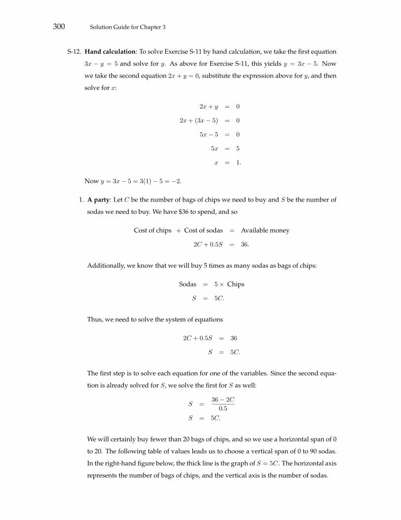
300 Solution Guide for Chapter 3
S-12. Hand calculation: To solve Exercise S-11 by hand calculation, we take the first equation
3x − y = 5 and solve for y. As above for Exercise S-11, this yields y = 3x − 5. Now
we take the second equation 2x + y = 0, substitute the expression above for y, and then
solve for x:
2x + y = 0
2x + (3x− 5) = 0
5x− 5 = 0
5x = 5
x = 1.
Now y = 3x− 5 = 3(1)− 5 = −2.
1. A party: Let C be the number of bags of chips we need to buy and S be the number of
sodas we need to buy. We have $36 to spend, and so
Cost of chips + Cost of sodas = Available money
2C + 0.5S = 36.
Additionally, we know that we will buy 5 times as many sodas as bags of chips:
Sodas = 5× Chips
S = 5C.
Thus, we need to solve the system of equations
2C + 0.5S = 36
S = 5C.
The first step is to solve each equation for one of the variables. Since the second equa-
tion is already solved for S, we solve the first for S as well:
S =36− 2C
0.5S = 5C.
We will certainly buy fewer than 20 bags of chips, and so we use a horizontal span of 0
to 20. The following table of values leads us to choose a vertical span of 0 to 90 sodas.
In the right-hand figure below, the thick line is the graph of S = 5C. The horizontal axis
represents the number of bags of chips, and the vertical axis is the number of sodas.

SECTION 3.5 Systems of Equations 301
We see that the graphs cross at C = 8 and S = 40. This means that we should buy 8
bags of chips and 40 sodas.
2. Mixing feed:
(a) In the 30 pounds of alfalfa there are
20% of 30 = 0.20× 30 = 6 pounds of protein.
In the 40 pounds of wheat mids there are
15% of 40 = 0.15× 40 = 6 pounds of protein.
So altogether there are 12 pounds of protein in the mixture.
(b) We have
Total protein = 20% of alfalfa + 15% of wheat mids
Total protein = 0.20a + 0.15w.
(c) We want a total of 17% protein in the 1000 pounds of feed. That means the feed
should contain 0.17 × 1000 = 170 pounds of protein. So from Part (b), we get the
equation
170 = 0.2a + 0.15w.
There are a total of 1000 pounds of cattle feed, and so
Total feed = alfalfa + wheat mids
1000 = a + w.
Thus, we need to solve the system of equations
170 = 0.2a + 0.15w
1000 = a + w.
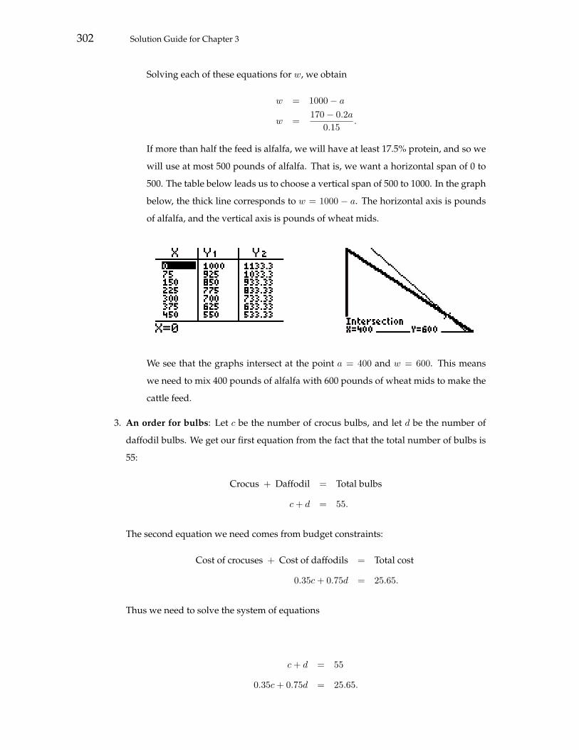
302 Solution Guide for Chapter 3
Solving each of these equations for w, we obtain
w = 1000− a
w =170− 0.2a
0.15.
If more than half the feed is alfalfa, we will have at least 17.5% protein, and so we
will use at most 500 pounds of alfalfa. That is, we want a horizontal span of 0 to
500. The table below leads us to choose a vertical span of 500 to 1000. In the graph
below, the thick line corresponds to w = 1000 − a. The horizontal axis is pounds
of alfalfa, and the vertical axis is pounds of wheat mids.
We see that the graphs intersect at the point a = 400 and w = 600. This means
we need to mix 400 pounds of alfalfa with 600 pounds of wheat mids to make the
cattle feed.
3. An order for bulbs: Let c be the number of crocus bulbs, and let d be the number of
daffodil bulbs. We get our first equation from the fact that the total number of bulbs is
55:
Crocus + Daffodil = Total bulbs
c + d = 55.
The second equation we need comes from budget constraints:
Cost of crocuses + Cost of daffodils = Total cost
0.35c + 0.75d = 25.65.
Thus we need to solve the system of equations
c + d = 55
0.35c + 0.75d = 25.65.

SECTION 3.5 Systems of Equations 303
Solving each of these equations for d, we get
d = 55− c
d =25.65− 0.35c
0.75.
Since there are certainly no more than 55 crocus bulbs, we use a horizontal span of 0
to 55. From the table below, we choose a vertical span of 0 to 35. In the graph below,
the thick line corresponds to d =25.65− 0.35c
0.75. The horizontal axis is the number of
crocus bulbs, and the vertical axis is the number of daffodil bulbs.
We see that the graphs intersect at the point c = 39 and d = 16. So we should buy 39
crocus bulbs and 16 daffodil bulbs.
4. American dollars and British pounds: Let p be the number of British pound notes,
and let d be the number of American dollars. We get the first equation from the total
number of bills:
Number of pounds + Number of dollars = Total bills
p + d = 17.
The second equation comes from the total value (in American dollars) in the wallet:
Value of pounds + Value of dollars = Total value
2.66p + d = 30.28.
Hence we need to solve the system of equations
p + d = 17
2.66p + d = 30.28.
Solving both of these equations for d yields
d = 17− p
d = 30.28− 2.66p.

304 Solution Guide for Chapter 3
Since there are 17 bills altogether, we use a horizontal span of 0 to 17. The table of
values below leads us to choose a vertical span of 0 to 35. The thick line in the graph
below corresponds to d = 30.38− 2.66p. The horizontal axis is pounds, and the vertical
axis is dollars.
We see that the graphs intersect at the point p = 8 and d = 9. So we have 8 British
pound notes and 9 American dollars.
5. Population growth: Let f be the number of foxes and r the number of rabbits. Since
the rates of change for both foxes and rabbits are constant (33 per year and 53 per year
respectively), both are linear functions of time. After t years, there will be f = 255+33t
foxes and r = 104 + 53t rabbits. We want to know when these values will be the same.
That is, we need to find out when f = r, or when 255 + 33t = 104 + 53t. This is a linear
equation which we can solve by hand calculation or by graphing. Here is the hand
calculation:
255 + 33t = 104 + 53t
151 + 33t = 53t Subtract 104 from each side.
151 = 20t Subtract 33t from both sides.
7.55 = t Divide each side by 20.
Hence, the number of foxes will be the same as the number of rabbits in 7.55 years. At
that time, there will be f = 255 + 33× 7.55 = 504.15 foxes (this is better reported as 504
foxes) and the same number of rabbits.
6. Teacher salaries: We begin by calculating the regression lines. For elementary teachers,
the regression line is E = 0.98t + 35.24, where t is years since 1994 and E is the salary,
in thousands of dollars, of elementary teachers. For secondary teachers, the regression
line is S = 0.82t + 36.66, where t is years since 1994 and S is the salary, in thousands of
dollars, of secondary teachers. We want to know when these values will be the same.
That is, we need to find out when E = S, or when 0.98t + 35.24 = 0.82t + 36.66. This is
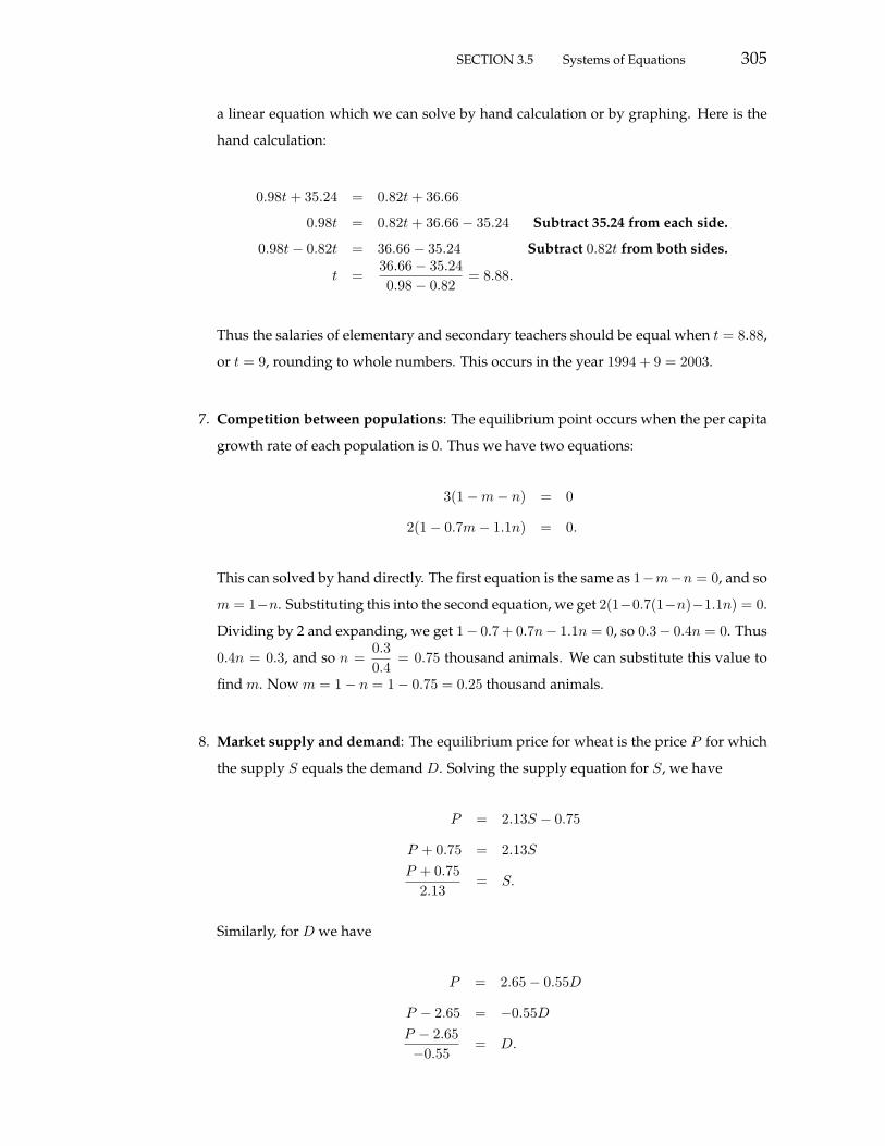
SECTION 3.5 Systems of Equations 305
a linear equation which we can solve by hand calculation or by graphing. Here is the
hand calculation:
0.98t + 35.24 = 0.82t + 36.66
0.98t = 0.82t + 36.66− 35.24 Subtract 35.24 from each side.
0.98t− 0.82t = 36.66− 35.24 Subtract 0.82t from both sides.
t =36.66− 35.240.98− 0.82
= 8.88.
Thus the salaries of elementary and secondary teachers should be equal when t = 8.88,
or t = 9, rounding to whole numbers. This occurs in the year 1994 + 9 = 2003.
7. Competition between populations: The equilibrium point occurs when the per capita
growth rate of each population is 0. Thus we have two equations:
3(1−m− n) = 0
2(1− 0.7m− 1.1n) = 0.
This can solved by hand directly. The first equation is the same as 1−m−n = 0, and so
m = 1−n. Substituting this into the second equation, we get 2(1−0.7(1−n)−1.1n) = 0.
Dividing by 2 and expanding, we get 1− 0.7 + 0.7n− 1.1n = 0, so 0.3− 0.4n = 0. Thus
0.4n = 0.3, and so n =0.30.4
= 0.75 thousand animals. We can substitute this value to
find m. Now m = 1− n = 1− 0.75 = 0.25 thousand animals.
8. Market supply and demand: The equilibrium price for wheat is the price P for which
the supply S equals the demand D. Solving the supply equation for S, we have
P = 2.13S − 0.75
P + 0.75 = 2.13S
P + 0.752.13
= S.
Similarly, for D we have
P = 2.65− 0.55D
P − 2.65 = −0.55D
P − 2.65−0.55
= D.

306 Solution Guide for Chapter 3
Now the equilibrium price is when S = D, so we have
S = D
P + 0.752.13
=P − 2.65−0.55
−0.55(P + 0.75) = 2.13(P − 2.65) Multiplying by (−0.55)× 2.13
−0.55P − 0.55× 0.75 = 2.13P − 2.13× 2.65
−0.55P − 2.13P = 0.55× 0.75− 2.13× 2.65
P =0.55× 0.75− 2.13× 2.65
−0.55− 2.13= 1.95.
So the equilibrium price for wheat is $1.95 per bushel. This can also be found by graph-
ing.
9. Boron uptake:
(a) The amount of water-soluble boron B available resulting in the same plant content
of boron for Decatur silty clay and Hartsells fine sandy loam is where 33.78 +
37.5B = 31.22 + 71.17B. You can solve this problem graphically, using a table, or
calculating it by hand. By hand, we move terms to the same side to get 33.78 −
31.22 = 71.17B − 37.5B = (71.17 − 37.5)B. Thus B =33.78− 31.2271.17− 37.5
= 0.08 part
per million.
(b) The value of boron B from Part (a) gives the same plant content C for either soil
type. For the Hartsells fine sandy loam, C increases by 71.17 parts per million with
each increase of 1 in B, whereas for the Decatur silty clay, C only increases by 37.5
parts per million with each increase of 1 in B. Thus if B is larger than 0.08 part per
million, the Hartsells fine sandy loam will have the larger plant content of boron.

SECTION 3.5 Systems of Equations 307
10. Male and female high school graduates:
(a) From the left-hand figure below, we see that the regression line is Y = −0.126X +
55.72, where X is the number of years since 1960 and Y is the percentage of male
high school graduates enrolled in college.
(b) The right-hand figure below shows that the regression line is Y = 0.73X + 39.7,
where X is the number of years since 1960 and Y is the percentage of female high
school graduates enrolled in college.
(c) To find out when percentages of males and females are the same, we graph both
regression lines and find the intersection point. (This can also be done by hand
calculation.) The table of values below leads us to choose a horizontal span of 0 to
30 and a vertical span of 30 to 60. In the graph below, the thick line corresponds to
the percentage of females. The horizontal axis is the number of years since 1960,
and the vertical axis is the percentage enrolling in college.
We see that the graphs intersect when X = 18.71 and Y = 53.36. So we would ex-
pect to see the same percentage, 53.36%, of male and female high school graduates
entering college at the time 18.72 years after 1960, or in about 1979.

308 Solution Guide for Chapter 3
11. Fahrenheit and Celsius: When Fahrenheit is exactly twice as much as Celsius, we have
F = 2C. That means we need to solve the system of equations
F =95C + 32
F = 2C.
Since both equations are already solved for F , we need only graph both functions and
find the intersection. The table of values below leads us to choose a horizontal span of
150 to 200 and a vertical span of 300 to 400. In the graph below, the thick line corre-
sponds to F = 2C. The horizontal axis is Celsius temperature, and the vertical axis is
Fahrenheit temperature.
We see that the graphs intersect when C = 160 and F = 320. Thus the temperature we
seek is 160 degrees Celsius and 320 degrees Fahrenheit.
12. A bag of coins: Let D be the number of dimes and Q the number of quarters. Since
there are 30 coins, D+Q = 30. Since the value of the coins is $3.45, 0.10D+0.25Q = 3.45.
The first equation can easily be solved for Q, giving Q = 30 −D. Substituting into the
second equation, we get
0.10D + 0.25Q = 3.45
0.10D + 0.25(30−D) = 3.45
0.10D + 0.25× 30− 0.25D = 3.45
0.10D − 0.25D = 3.45− 0.25× 30
D =3.45− 0.25× 30
0.10− 0.25= 27.
Thus the bag contains 27 dimes and 3 quarters.
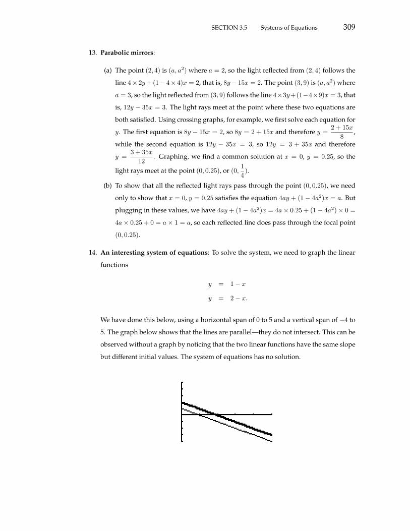
SECTION 3.5 Systems of Equations 309
13. Parabolic mirrors:
(a) The point (2, 4) is (a, a2) where a = 2, so the light reflected from (2, 4) follows the
line 4× 2y + (1− 4× 4)x = 2, that is, 8y− 15x = 2. The point (3, 9) is (a, a2) where
a = 3, so the light reflected from (3, 9) follows the line 4×3y+(1−4×9)x = 3, that
is, 12y − 35x = 3. The light rays meet at the point where these two equations are
both satisfied. Using crossing graphs, for example, we first solve each equation for
y. The first equation is 8y − 15x = 2, so 8y = 2 + 15x and therefore y =2 + 15x
8,
while the second equation is 12y − 35x = 3, so 12y = 3 + 35x and therefore
y =3 + 35x
12. Graphing, we find a common solution at x = 0, y = 0.25, so the
light rays meet at the point (0, 0.25), or (0,14).
(b) To show that all the reflected light rays pass through the point (0, 0.25), we need
only to show that x = 0, y = 0.25 satisfies the equation 4ay + (1 − 4a2)x = a. But
plugging in these values, we have 4ay + (1− 4a2)x = 4a× 0.25 + (1− 4a2)× 0 =
4a× 0.25 + 0 = a× 1 = a, so each reflected line does pass through the focal point
(0, 0.25).
14. An interesting system of equations: To solve the system, we need to graph the linear
functions
y = 1− x
y = 2− x.
We have done this below, using a horizontal span of 0 to 5 and a vertical span of −4 to
5. The graph below shows that the lines are parallel—they do not intersect. This can be
observed without a graph by noticing that the two linear functions have the same slope
but different initial values. The system of equations has no solution.

310 Solution Guide for Chapter 3
15. Another interesting system of equations: Solving both equations for y, we see that we
need to graph the two functions
y =3− x
2
y =6− 2x
4.
If we do this, we find that both graphs produce the same line, showing that the two
functions are in fact identical. If you divide the equation −2x− 4y = −6 by −2, you get
the equation x + 2y = 3, which is exactly the first equation. Since the two equations are
the same, every point on the line x + 2y = 3 is also on the other line, and hence every
such point is a solution of the system of equations.
16. A system of three equations in three unknowns:
(a) We get z = 3− 2x + y.
(b) We get the system of equations
x + y + 2(3− 2x + y) = 9
3x + 2y − (3− 2x + y) = 4.
Solving both of these equations for y, we get the following system:
y = 1 + x
y = 7− 5x.
(c) If we graph both of the equations in Part (b) using both a horizontal and a vertical
span of −10 to 10, we get the picture below.
We see that the graphs intersect when x = 1 and y = 2.
(d) From Part (a) we know that z = 3 − 2x + y. Since x = 1 and y = 2, we get
z = 3 − 2 × 1 + 2 = 3. So the solution of the system of equations is x = 1, y = 2
and z = 3.

SECTION 3.5 Systems of Equations 311
17. An application of three equations in three unknowns: Let N be the number of nickels,
D the number of dimes, and Q the number of quarters. Since there are 21 coins in the
bag, N + D + Q = 21. Since there is one more dime than nickel in the bag, D = N + 1.
Since there is $3.35 in the bag, 0.05N + 0.10D + 0.25Q = 3.35.
This gives three linear equations in the variables N , D, and Q:
N + D + Q = 21
D = N + 1
0.05N + 0.10D + 0.25Q = 3.35.
The second equation is already solved for D, so we will substitute that into the other
two equations. The first equation becomes N + (N + 1) + Q = 21, or 2N + Q + 1 = 21.
Solving for Q, we get Q = 20− 2N .
The third equation becomes 0.05N + 0.10(N + 1) + 0.25Q = 3.35, or 0.05N + 0.10N +
0.10 + 0.25Q = 3.35. Solving for Q gives
Q =3.25− 0.15N
0.25.
Graphing both of these equations using a horizontal span from 0 to 10 nickels and a
vertical span from 0 to 30 quarters yields the following picture.
The graphs intersect when N = 5 and Q = 10.
We know that D = N + 1. Since N = 5, D = 5 + 1 = 6. So the solution to the equation
is N = 5, D = 6, and Q = 10: there are 5 nickels, 6 dimes, and 10 quarters.

312 Solution Guide for Chapter 3
Chapter 3 Review Exercises
1. Drainage pipe slope: We have Slope =RiseRun
. In this case, the rise is −0.5 foot (since 6
inches make 0.5 foot) for a run of 8 feet. Thus the slope is−0.5
8= −0.0625 foot per foot.
If we measure the rise in inches then we find−68
= −0.75 inch per foot for the slope.
2. Height from slope and horizontal distance: We have
Vertical change = Slope × Horizontal change.
In this case, the slope of the ladder is 3.7, while the horizontal distance is 4.4 feet, so the
vertical height is 3.7× 4.4 = 16.28 feet.
3. A ramp into a van:
(a) We have Slope =RiseRun
. In this case, the rise is 18 inches, the distance from the van
door to the ground, and the run is 4 feet, since that is the horizontal distance from
the ramp to the van. Thus the slope is184
= 4.5 inches per foot. If we measure the
rise in feet then we find1.54
= 0.375 foot per foot for the slope.
(b) We have
Rise = Slope × Run.
In this case we take the slope to be 1.2 inches per foot. The rise is still 18 inches, so
we have 18 = 1.2× Run. Thus the run is181.2
= 15 feet. A larger slope will require
a greater distance, so the ramp should rest at least 15 feet from the van.
4. A reception tent:
(a) We have Slope =RiseRun
. The rise from the top of an outside pole to the top of the
center pole is 25 − 10 = 15 feet, and the corresponding run is 30 feet. Thus the
slope is1530
= 0.5 foot per foot.
(b) We have
Rise = Slope × Run.
We know from Part (a) that the slope is 0.5 foot per foot. The run is 5 feet, so the
rise is 0.5× 5 = 2.5 feet. Thus the height has increased by 2.5 feet from the outside
poles. We add the height of an outside pole to get that the height at this point is
2.5 + 10 = 12.5 feet.

Chapter 3 Review Exercises 313
(c) We have
Rise = Slope × Run.
We know from Part (a) that the slope is 0.5 foot per foot. The rise from the ground
to the top of an outer pole is 10 feet, so we have 10 = 0.5 × Run. Thus the run is100.5
= 20 feet. Hence the ropes are attached to the ground 20 feet from the outside
poles.
5. Function value from slope and run: We have that the slope is m = −2.2, so
−2.2 =Change in functionChange in variable
=g(6.8)− g(3.7)
6.8− 3.7=
g(6.8)− 5.16.8− 3.7
=g(6.8)− 5.1
3.1.
Thus g(6.8)− 5.1 = 3.1× (−2.2), and so g(6.8) = 5.1− 3.1× (−2.2) = −1.72.
6. Lanes on a curved track:
(a) To find the inner radius of the first lane, we put n = 1 in the formula and find
R(1) = 100/π. Thus the radius is about 31.83 meters.
(b) The width of a lane is the change in R when we increase n by 1, and that is the
slope of the linear function R. From the formula we see that the slope is 1.22. Thus
the width of a lane is 1.22 meters. This can also be found by subtracting successive
values of the radius; for example, R(2)−R(1) = 1.22.
(c) We first find for what value of n we have R(n) = 35. This means we must solve
the linear equation 100/π + 1.22(n− 1) = 35 for n. We have
100/π + 1.22(n− 1) = 35
1.22(n− 1) = 35− 100/π
n− 1 =35− 100/π
1.22n =
35− 100/π
1.22+ 1 = 3.60.
Since the number of lanes is a whole number, if you wish to run in a lane with a
radius of at least 35 meters you should pick lane 4 or a higher-numbered lane.
7. Linear equation from two points: We first compute the slope:
m =Change in functionChange in variable
=g(1.1)− g(−2)
1.1− (−2)=
3.3− 7.23.1
=−3.93.1
= −1.258.
(We keep the extra digit for accuracy in the rest of the calculations.) Since g is a linear
function with slope −1.258, we have g = −1.258x + b for some b. Now g(1.1) = 3.3, so
3.3 = −1.258×1.1+ b, and therefore b = 3.3+1.258×1.1 = 4.68. Thus if we now round
the slope to 2 decimal places we get g = −1.26x + 4.68.

314 Solution Guide for Chapter 3
8. Working on a commission:
(a) Each additional dollar of total sales increases the income by 5% of $1, or 0.05 dollar.
This means that the change in I is always the same, 0.05 dollar, for a change of 1
in S. Thus I is a linear function of S.
(b) If he sells $1600 in a month then he earns $1000 plus 5% of $1600, or 1000 + 0.05×
1600 = 1080 dollars.
(c) From Part (a), I is a linear function of S with slope 0.05, since the slope represents
the additional income for 1 additional dollar in sales. Since I is a linear function
with slope 0.05, we have I = 0.05S + b for some b. Now I(1600) = 1080 by Part
(b), so 1080 = 0.05× 1600 + b, and therefore b = 1080− 0.05× 1600 = 1000. Thus
I = 0.05S + 1000.
(d) We want to find the value of S so that I = 1350. That means we need to solve the
equation 0.05S + 1000 = 1350 for S. We find:
0.05S + 1000 = 1350
0.05S = 1350− 1000
S =1350− 1000
0.05= 7000.
Thus his monthly sales must be $7000.
9. Testing data for linearity:
(a) There is a constant change of 0.3 in x and a constant change of −0.06 in f . Thus
these data exhibit a constant rate of change and so are linear.
(b) From Part (a) we know that the data show a constant rate of change of −0.6 in
f per change of 0.3 in x. Hence the slope is m =Change in f
Change in x=
−0.60.3
= −2.
We know now that f = −2x + b for some b. Since f = 8 when x = 3, we have
8 = −2× 3 + b, so b = 8 + 2× 3 = 14. The formula is f = −2x + 14.
10. An epidemic:
(a) There is a constant change of 5 in d and a constant change of 6 in T . Thus these
data exhibit a constant rate of change and so are linear.
(b) The slope represents the number of new cases per day.
(c) The slope is m =Change in T
Change in d=
65
= 1.2.
(d) Now T is a linear function with slope 1.2, and the initial value is 35 (from the first
entry in the table). Thus the formula is T = 1.2d + 35.

Chapter 3 Review Exercises 315
(e) To predict the total number of diagnosed flu cases after 17 days we put d = 17 in
the formula from Part (d): T = 1.2 × 17 + 35 = 55.4. Thus we expect 55 flu cases
to be diagnosed after 17 days.
11. Testing and plotting linear data:
(a) There is a constant change of 2 in x and a constant change of 0.24 in f . Thus these
data exhibit a constant rate of change and so are linear.
(b) The slope is m =Change in f
Change in x=
0.242
= 0.12. We know now that f = 0.12x + b
for some b. Since f = −1.12 when x = −1, we have −1.12 = 0.12 × (−1) + b, so
b = −1.12 + 0.12 = −1. The formula is f = 0.12x− 1.
(c) The figure below shows the plot of the data together with the graph of f = 0.12x−
1.
12. Marginal tax rate:
(a) There is a constant change of $50 in the taxable income and a constant change of
$14 in the tax due. Thus these data exhibit a constant rate of change and so are
linear.
(b) From Part (a) the rate of change in tax due as a function of taxable income is1450
=
0.28 dollar per dollar. Thus the additional tax due on each dollar is $0.28.
(c) From the table the tax due on a taxable income of $97,000 is $21,913. If the taxable
income increases by $1000 to $98,000, by Part (b) the tax due will increase by 0.28×
1000 = 280 dollars. Thus the tax due on a taxable income of $98,000 is 21,913 +
280 = 22,913 dollars.
(d) Let T denote the tax due, in dollars, on an income of A dollars over $97,000. The
slope of T is 0.28 by Part (b). The initial value of T is the tax due on 0 dollars
over $97,000, that is, on $97,000. That tax is $21,913. Thus the formula is T =
0.28A + 21,913.

316 Solution Guide for Chapter 3
13. Plotting data and regression lines:
(a) The figure below on the left is a plot of the data.
(b) The regression line is y = −16.3x + 37.19.
(c) The figure on the right below is the plot of the data with the regression line added.
14. Meaning of slope of regression line: If the slope of the regression line for number of
births per thousand to unmarried 18- to 19-year-old women as a function of year is
−1.13, then for each year that passes the number of births to unmarried 18- to 19-year
old women decreases by about 1.16 births per thousand.
15. Life expectancy:
(a) Let E be life expectancy in years and t the time in years since 1996. Using regres-
sion gives the model E = 0.2t + 76.2.
(b) The figure below is the plot of the data with the regression line added.
(c) The slope of the regression line is 0.2, and this means that for each increase of 1 in
the year of birth the life expectancy increases by 0.2 year, or about 2 12 months.

Chapter 3 Review Exercises 317
(d) Now 2005 corresponds to t = 9, so using the regression line we predict the life
expectancy to be 0.2× 9 + 76.2 = 78 years.
(e) Now 1580 corresponds to t = −416, so from the regression line we expect the life
expectancy to be 0.2×(−416)+76.2 = −7 years. This is nonsensical! The year 2300
corresponds to t = 304, so from the regression line we predict the life expectancy
to be 0.2 × 304 + 76.2 = 137 years. This is unreasonable. In fact, both of these
predictions are far out of the range of applicability of the regression line formula.
16. XYZ Corporation stock prices:
(a) Let P be the stock price in dollars and t the time in months since January, 2005.
Using regression gives the model P = 0.547t + 43.608.
(b) The figure below is the plot of the data with the regression line added.
(c) The slope is 0.547 dollar per month, and this means that the stock price increases
by about $0.55 each month.
(d) Now January, 2006 corresponds to t = 12, so using the regression line we predict
the stock price to be 0.547 × 12 + 43.608 = 50.172, or about $50.17. Also January,
2007 corresponds to t = 24, so using the regression line we predict the stock price
to be 0.547× 24 + 43.608 = 56.736, or about $56.74.

318 Solution Guide for Chapter 3
17. Crossing graphs: We start with
4x− 2y = 9
x + y = 0
and solve each equation for y. For the first equation we have 4x−2y = 9, so 2y = 4x−9
and therefore y =4x− 9
2. For the second equation we have x + y = 0, so y = −x. The
figure below shows the graph of both y =4x− 9
2and y = −x using a horizontal span
of 0 to 2 and a vertical span of −5 to 0. The intersection point, which is the solution to
the system, is at x = 1.5, y = −1.5.
18. Hand calculation: To solve Exercise 17 by hand calculation, we take the second equa-
tion x + y = 0 and solve for y. As above for Exercise 17, this yields y = −x. Now we
take the first equation 4x−2y = 9, substitute the expression above for y, and then solve
for x:
4x− 2y = 9
4x− 2(−x) = 9
6x = 9
x =96
= 1.5.
Now y = −x = −1.5.
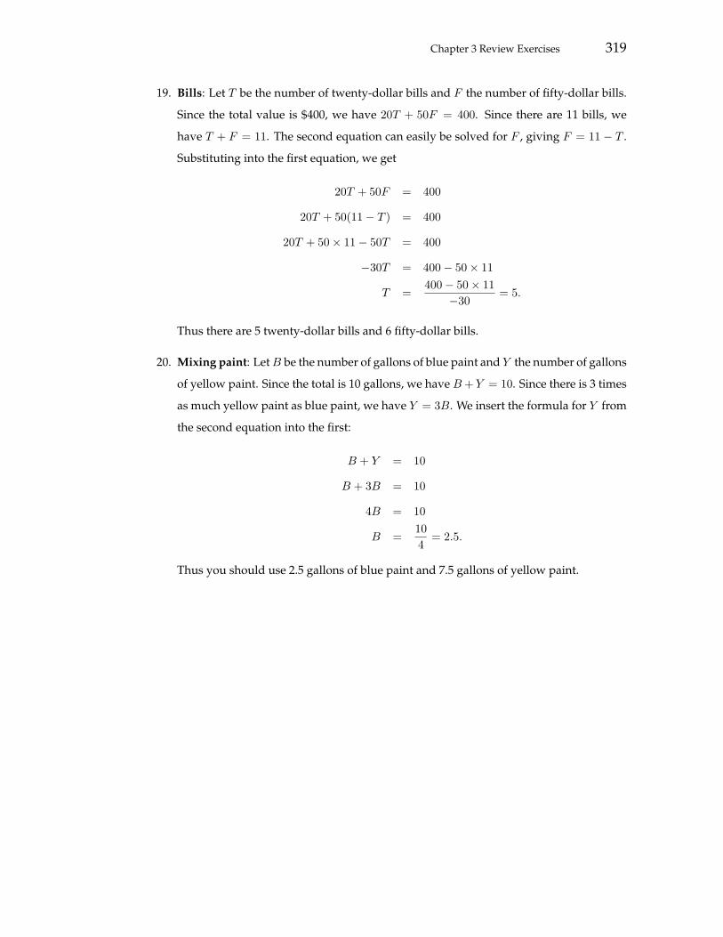
Chapter 3 Review Exercises 319
19. Bills: Let T be the number of twenty-dollar bills and F the number of fifty-dollar bills.
Since the total value is $400, we have 20T + 50F = 400. Since there are 11 bills, we
have T + F = 11. The second equation can easily be solved for F , giving F = 11 − T .
Substituting into the first equation, we get
20T + 50F = 400
20T + 50(11− T ) = 400
20T + 50× 11− 50T = 400
−30T = 400− 50× 11
T =400− 50× 11
−30= 5.
Thus there are 5 twenty-dollar bills and 6 fifty-dollar bills.
20. Mixing paint: Let B be the number of gallons of blue paint and Y the number of gallons
of yellow paint. Since the total is 10 gallons, we have B + Y = 10. Since there is 3 times
as much yellow paint as blue paint, we have Y = 3B. We insert the formula for Y from
the second equation into the first:
B + Y = 10
B + 3B = 10
4B = 10
B =104
= 2.5.
Thus you should use 2.5 gallons of blue paint and 7.5 gallons of yellow paint.