Delft University of Technology

Solubility of water in hydrogen at high pressuresA molecular simulation studyRahbari, Ahmadreza; Brenkman, Jeroen; Hens, Remco; Ramdin, Mahinder; Van Den Broeke, Leo J.P.;Schoon, Rogier; Henkes, Ruud; Moultos, Othonas A.; Vlugt, Thijs J.H.DOI10.1021/acs.jced.9b00513Publication date2019Document VersionFinal published versionPublished inJournal of Chemical and Engineering Data

Citation (APA)Rahbari, A., Brenkman, J., Hens, R., Ramdin, M., Van Den Broeke, L. J. P., Schoon, R., Henkes, R.,Moultos, O. A., & Vlugt, T. J. H. (2019). Solubility of water in hydrogen at high pressures: A molecularsimulation study. Journal of Chemical and Engineering Data, 64(9), 4103-4115.https://doi.org/10.1021/acs.jced.9b00513Important noteTo cite this publication, please use the final published version (if applicable).Please check the document version above.

CopyrightOther than for strictly personal use, it is not permitted to download, forward or distribute the text or part of it, without the consentof the author(s) and/or copyright holder(s), unless the work is under an open content license such as Creative Commons.

Takedown policyPlease contact us and provide details if you believe this document breaches copyrights.We will remove access to the work immediately and investigate your claim.

This work is downloaded from Delft University of Technology.For technical reasons the number of authors shown on this cover page is limited to a maximum of 10.

Solubility of Water in Hydrogen at High Pressures: A MolecularSimulation StudyAhmadreza Rahbari,† Jeroen Brenkman,‡ Remco Hens,† Mahinder Ramdin,†

Leo J. P. van den Broeke,† Rogier Schoon,‡ Ruud Henkes,‡ Othonas A. Moultos,†

and Thijs J. H. Vlugt*,†

†Engineering Thermodynamics, Process & Energy Department, Faculty of Mechanical, Maritime and Materials Engineering, DelftUniversity of Technology, Leeghwaterstraat 39, 2628CB, Delft, The Netherlands‡Shell Global Solutions International, PO Box 38000, 1030BN, Amsterdam, The Netherlands

*S Supporting Information

ABSTRACT: Hydrogen is one of the most popular alternativesfor energy storage. Because of its low volumetric energy density,hydrogen should be compressed for practical storage andtransportation purposes. Recently, electrochemical hydrogencompressors (EHCs) have been developed that are capable ofcompressing hydrogen up to P = 1000 bar, and have thepotential of reducing compression costs to 3 kWh/kg. As EHCcompressed hydrogen is saturated with water, the maximumwater content in gaseous hydrogen should meet the fuelrequirements issued by the International Organization forStandardization (ISO) when refuelling fuel cell electric vehicles.The ISO 14687−2:2012 standard has limited the waterconcentration in hydrogen gas to 5 μmol water per molhydrogen fuel mixture. Knowledge on the vapor liquid equilibrium of H2O−H2 mixtures is crucial for designing a method toremove H2O from compressed H2. To the best of our knowledge, the only experimental high pressure data (P > 300 bar) forthe H2O−H2 phase coexistence is from 1927 [J. Am. Chem. Soc., 1927, 49, 65−78]. In this paper, we have used molecularsimulation and thermodynamic modeling to study the phase coexistence of the H2O−H2 system for temperatures between T =283 K and T = 423 K and pressures between P = 10 bar and P = 1000 bar. It is shown that the Peng-Robinson equation of stateand the Soave Redlich-Kwong equation of state with van der Waals mixing rules fail to accurately predict the equilibriumcoexistence compositions of the liquid and gas phase, with or without fitted binary interaction parameters. We have shown thatthe solubility of water in compressed hydrogen is adequately predicted using force-field-based molecular simulations. Themodeling of phase coexistence of H2O−H2 mixtures will be improved by using polarizable models for water. In the SupportingInformation, we present a detailed overview of available experimental vapor−liquid equilibrium and solubility data for theH2O−H2 system at high pressures.

1. INTRODUCTION

The world population is expected to grow rapidly, from 7.6billion currently, to about 9.8 billion in 2050.1 Due toincreasing prosperity, the worldwide consumption of energyper individual will also increase. Even in the current modernworld, several billion people still do not have access to basicneeds, such as clean water, sanitation, nutrition, health care,and education.2 These are all examples of the SustainableDevelopment Goals, adopted by all United Nations MemberStates in 2015.2 Access to energy is a key enabler to reach thesebasic needs. The worldwide energy demand is thereforeexpected to increase by 40% by 2040.3 At the same time, CO2

emissions need to be reduced to reach the goals of the Parisagreement.4 Roughly, 80% of the total primary energy supply iscurrently produced by fossil fuels, such as coal, oil, and naturalgas.3 To reach the goals of the Paris agreement, attempts have

been made to replace fossil fuels with renewable alternativessuch as wind and solar (PV) energy. Current expectations arethat by 2040, 40% of the total generated electricity will be fromrenewable energy sources.3

Unlike fossil fuels, energy production from intermittentrenewable sources, including wind power and solar energy,critically depend on the availability of these sources leading toan uncontrollable energy output.5 For direct integration to thepower grid, uncontrollable availability of intermittent renew-able energy sources within 10% of the installed capacity isacceptable without major technical problems.5 However, largescale integration of intermittent energy sources above this limit

Received: June 4, 2019Accepted: August 13, 2019Published: August 26, 2019

Article

pubs.acs.org/jcedCite This: J. Chem. Eng. Data 2019, 64, 4103−4115

© 2019 American Chemical Society 4103 DOI: 10.1021/acs.jced.9b00513J. Chem. Eng. Data 2019, 64, 4103−4115

This is an open access article published under a Creative Commons Non-Commercial NoDerivative Works (CC-BY-NC-ND) Attribution License, which permits copying andredistribution of the article, and creation of adaptations, all for non-commercial purposes.

Dow

nloa

ded

via

TU

DE

LFT

on

Oct

ober

1, 2

019

at 1

4:00

:12

(UT

C).

See

http

s://p

ubs.

acs.

org/

shar

ingg

uide

lines

for

opt

ions

on

how

to le

gitim

atel

y sh

are

publ

ishe

d ar

ticle

s.

is expected to cause frequent mismatches between the supplyand demand of energy. To avoid this, the integration of energystorage technologies is proposed as one of the promisingsolutions for stable and flexible supply of electricity.6,7

Different types of technologies have been developed forelectrical energy storage including: hydrostorage, flywheels,batteries, and hydrogen produced by electrolysis, etc.5,6,8,9 Oneof the most popular alternatives for energy storage ishydrogen.8 Hydrogen has the advantage that it can be storedfor long periods and converted to electricity withoutpollution.10 Hydrogen has a broad span of applications, suchas fuel cells, fuel for heating, transportation, or even as a rawmaterial for the chemical industry.5,10,11 Since hydrogen has avery low density at standard conditions, it has a very lowvolumetric energy density. For practical storage and trans-portation purposes, the density of hydrogen must be increasedsignificantly.12 The density of hydrogen can be increased bycompression, cooling, or a combination of both, depending onthe scale and application.12 One of the emerging applicationsfor hydrogen is found in sustainable transportation.10 In fuelcell electric vehicles (FCEV), hydrogen is stored in com-pressed form in pressurized cylinders at P = 350 bar or P = 700bar.12 In practice, a passenger car needs a tank capacity of ca.100 to 150 L to store 4 to 6 kg of hydrogen, which provides arange of approximately 500 km.12 High pressure storage tankswith pressures of at least P = 875 bar12,13 are installed atrefuelling stations, to fuel a vehicle within the target time of 3to 5 min.12 Conventional compressor types that are currentlyused are piston, compressed air, diaphragm, or ioniccompressors, depending mainly on the capacity of therefuelling station.12 The conventional compressor requires onaverage 6 kWh/kg of energy to compress hydrogen from 10 to400 bar.13

An alternative compressor is the electrochemical hydrogencompressor (EHC). HyET Hydrogen BV14 has developed anEHC that works with pressures up to 1000 bar, and has thepotential of bringing compression costs down to 3 kWh/kg.13

The working principle of an EHC operation is similar to aproton exchange membrane (PEM) fuel cell.15 A single EHCstack consists of a low pressure and a high pressure side,separated by a membrane that is only permeable for hydrogenprotons, and not for molecules. The membrane is positionedbetween two platinum catalysts containing electrodes. Once apotential difference is applied over the electrodes, a hydrogenmolecule splits into two protons. The protons then travelthrough the membrane where conversion to hydrogenmolecules takes place at elevated pressure.15 In the EHC, theproton transfer through the membrane is enabled by water.The EHC has several advantages compared to traditionaltechnologies:13,16−18 (1) The EHC has a higher efficiency,especially at high compression ratios.19 In theory, thecompression ratio using EHC can go to infinity, from anelectrochemical perspective. The mechanical strength and backdiffusion losses are the main limitations for higher pressureratios for the EHC.19 (2) Due to the highly selectivemembrane that only allows the permeation of protons,contaminants are prevented from passing the membrane.19

This means that the EHC performs both as a compressor and apurifier of hydrogen gas.19 (3) The compressor has no movingparts, resulting in lower maintenance costs and makinglubricants, which may contaminate the compressed hydrogen,redundant. (4) The EHC operates silently, since it has norotating parts. This makes the EHC suitable for locations such

as refuelling stations, where acoustical emission is a constraint.(5) The EHC is a compact device that is well suited to scaleup.19 Disadvantages of the EHC are similar to those of fuelcells, mainly high material costs. For instance, the platinumcatalyst which is required to resist the corrosive environmentsin the compressor, is very expensive.19 Another disadvantage isrelated to the proton transport through the membrane. Waterenables the proton transport through the membrane, andtherefore the membrane always needs to be hydrated.20

Therefore, the resulting hydrogen gas is saturated with waterwhich can be an issue depending on the application. TheInternational Organization for Standardization (ISO) statedthat water provides a transport mechanism for water-solublecontaminants such as K+ and Na+ when present as anaerosol.21 Both K+ and Na+ can affect the fuel cell and are notrecommended to exceed 0.05 μmol K+ or Na+ per molhydrogen fuel mixture.21 To avoid potential issues, the ISO hasdirected the maximum allowed concentration of impurities forgaseous hydrogen, including water in Table 1 of the ISO14687-2:2012.21 The maximum concentration of water in thegaseous hydrogen, used for PEM fuel cells in road vehicles islimited to 5 μmol water per mol hydrogen fuel mixture.21 Thisposes two important questions. (1) What is the solubility ofwater in hydrogen at high pressures close to ambienttemperatures? (2) If this solubility is too large, what is thebest method to reduce the water content? To answer thesequestions, an accurate description of the vapor liquidequilibrium (VLE) of the H2O−H2 system at high pressuresis required. Published experimental data that describe thesesystems is scarce. To the best of our knowledge, the onlyexperimental data describing phase coexistence of H2O−H2 forpressures exceeding 300 bar are from 1927 (limited to T = 323K22). At this temperature, hydrogen is supercritical. Wiebe andGaddy studied also the solubility of hydrogen gas in liquidwater at high pressures up to P = 1013.25 bar.23 Therefore,molecular simulation and thermodynamic modeling areneeded to determine the water content in compressedhydrogen. In industrial applications, cubic type equations ofstate (EoS) are one the most commonly used methods tostudy VLE, because of their simplicity.24−28 In this work, thePeng−Robinson (PR) EoS and the Soave−Redlich−Kwong(SRK) EoS with van der Waals mixing rules are used to predictthe phase coexistence of H2O−H2 at elevated pressures.However, molar volumes of the liquid phase and fugacitycoefficients at high pressures obtained from PR-EoS and SRK-EoS modeling are known to deviate significantly fromexperimental values.29−32

In this work, it is shown that both the PR-EoS and SRK-EoSfail to describe the liquid phase and the gas phasecompositions, with or without fitted binary interactionparameters (kij values). Since water is a highly polar molecule,either modifications of the conventional mixing rules arerequired,25 or more physically based models (i.e., SAFT-typesEoS33 or molecular simulations34) should be used to describethe phase behavior of the H2O−H2 system.33 It was found thata temperature-dependent parameter kij is still required forSAFT-type EoS modeling.35 Therefore, force-field-basedmolecular simulation could be considered as a natural tool tostudy the phase coexistence of the H2O−H2 system. In thiswork, different molecular force fields for water and hydrogenare considered for describing the phase coexistence composi-tions of the liquid and gas phase of the H2O− H2 system,especially at high pressures. To evaluate the accuracy of the

Journal of Chemical & Engineering Data Article

DOI: 10.1021/acs.jced.9b00513J. Chem. Eng. Data 2019, 64, 4103−4115

4104

results from molecular simulations, we have performed anextensive literature survey on the VLE of H2O−H2 mixtures athigh pressures.22,23,36−43 In this work, it is shown that the bestpredictions of the VLE of the H2O−H2 system at highpressures (in both phases) are obtained using molecularsimulations. No adjustable kij values were used for molecularsimulations in this study.This paper is organized as follows. In section 2, the

molecular simulation techniques used in this study areexplained and simulation details (molecular simulations andEoS modeling) and force field details for water and hydrogenare provided. Our results obtained from molecular simulationsand EoS modeling are presented and compared toexperimental data in section 3. Our conclusions aresummarized in section 4. In the Supporting Information, wepresent a detailed overview of available experimental VLE andsolubility data for the H2O−H2 system at high pressures.

2. MODELING AND METHODOLOGY2.1. Simulation Techniques. A convenient choice for

VLE calculations is the Gibbs Ensemble (GE) methodintroduced by Panagiotopoulos,44−46 which is used extensivelyin molecular simulation studies.34 In the GE, the vapor andliquid phase are simulated in two simulation boxes, which canexchange molecules, volume, and energy. At coexistence, thepressures, temperatures, and chemical potentials of eachcomponent are equal in both boxes.34 The GE is reliable,and the finite size effects are small unless conditions close tothe critical point are considered.47,48 To accurately predictcoexistence densities, simulations in the GE rely on sufficientmolecule exchanges between the two phases.34,45 The well-known drawback of the conventional GE is that at highdensities, particle insertions/deletions have a low acceptanceprobability, also leading to poor estimates of chemicalpotentials in both phases. Although chemical potentials ofdifferent component types are not strictly needed forcalculating the coexistence densities, the equality of chemicalpotentials is an important condition for phase equilibrium.Chemical potential calculations in the GE follow from amodification of the Widom’s Test Particle Insertion(WTPI),34,49 taking fluctuations in density into account. It iswell-known that the WTPI method often performs poorly fordense liquids.50,51

On the basis of the work of Shi and Maginn,52,53 Vlugt andco-workers expanded the conventional GE with so-calledfractional molecules to improve the efficiency of moleculeexchanges between the simulation boxes.54,55 In contrast to thenormal or “whole” molecules, the interactions of fractionalmolecules are scaled between zero and one with a couplingparameter λi. λi = 0 means that the fractional molecule of type ihas no interactions with the surrounding molecules and acts asan ideal gas molecule. λi = 1 means that the fractional moleculeof type i has fully scaled interactions and interacts as a wholemolecule. The fractional molecule of each component type canbe in either one of the phases.54 In addition to theconventional thermalization trial moves (translation, rotation,and volume changes), three additional trial moves areassociated with the fractional molecule of each component:(1) changes in λi while keeping the positions and orientationsof all molecules including the fractional molecule(s) fixed; (2)reinsertion of the fractional molecule to a randomly selectedposition in the other simulation box (phase) while keeping thevalue of λi, positions and orientations of all other molecules

fixed; (3) changing the identity of the fractional molecule witha randomly selected molecule of the same type in the otherbox, while keeping the value of λi, positions, and orientations ofall molecules fixed. Biasing using a weight function W(λi) isused to ensure that the observed probability distribution of λi isflat.54 The use of fractional molecules significantly improvesmolecule exchanges between the simulation boxes, and therebythe efficiency of the VLE calculations and the calculations ofchemical potentials at coexistence. When the number offractional molecules is less than 1% of the number of wholemolecules, the continuous fractional component GE (CFCGE)and the conventional GE yield identical coexistencedensities.56 Fractional molecules should not be countedwhen computing mole fractions.57 One can show thatcomputed chemical potentials in CFCGE and the conventionalGE are identical.54 For further details and a comparisonbetween the conventional GE and CFCGE, the reader isreferred to refs 50, 54, 58, and 59.Since molecule exchanges in the CFCGE are performed

using fractional molecules with scaled interactions, moleculetransfers between coexisting phases are facilitated leading to amore efficient sampling of coexistence densities. The chemicalpotential of component type i in phase j (gas or liquid) isobtained from54,55

i

kjjjjjj

y

{zzzzzzμ

ρ

ρ

λ

λ=

⟨ ⟩−

==

k T k Tp

pln ln

( 1)

( 0)ijij ij

ijB

0B

(1)

where kB is the Boltzmann constant, ρij is the number densityof component i in phase j and p(λij) is the (unbiased)Boltzmann probability distribution of λij in phase j. The termρ0 is an arbitrary reference density to make the argument of thelogarithm dimensionless. The first term on the right-hand sideof eq 1 is the ideal gas contribution of the chemical potential(μij

id). The second term on the right-hand side of eq 1 is theexcess chemical potential (μij

ex). The brackets ⟨···⟩ denote anensemble average. The fugacity coefficient of component type iin phase j follows from

ϕλ

λ= ×

==Z

p

p1 ( 0)

( 1)ijij

ijmix (2)

where Zmix is the compressibility factor of the mixture.Equation 2 is derived in the Supporting Information. On thebasis of the limited experimental solubility data available in theliterature at T = 323 K and pressures above P = 300 bar,22 weknow that the solubility of water in the gas phase at highpressures (P = 100 bar to P = 1000 bar) is about a couple ofhundred ppm’s (molar) or less. At lower temperatures, due tothe low solubility of water in hydrogen, a very large number ofhydrogen molecules (up to a million) in the gas phase wouldbe required in the simulations to have on average a single watermolecule in the gas phase. The solubility of hydrogen in theliquid phase is also very low, for example, mole fractionsranging from between 0.003 and 0.115 at T = 323 K andpressures between P = 25 bar and P = 1000 bar. This makesmost simulations of the H2O−H2 system in the CFCGE at lowtemperatures and high pressures impractical, as a very largesystem is needed to have at least a single component of eachtype in each box. One could in principle simulate the VLE ofH2O−H2 in the CFCGE using a smaller system size. Thiswould lead to poor statistics for the average number of H2molecules in the liquid phase, and H2O molecules in the gas

Journal of Chemical & Engineering Data Article

DOI: 10.1021/acs.jced.9b00513J. Chem. Eng. Data 2019, 64, 4103−4115

4105

phase. To circumvent these issues, both the gas and liquidphases (almost pure hydrogen gas and pure liquid water,respectively) are simulated independently in the continuousfractional component NPT (CFCNPT) ensemble.58 By varyingthe mixture composition in the gas and liquid phases aroundthe equilibrium state, the coexistence compositions areobtained by imposing equal chemical potentials for bothphases. Vlugt and co-workers considered the conventionalNPT ensemble expanded with a fractional molecule,58 similarto earlier work with the GE.54 Similar to the CFCGE, trialmoves for the fractional molecule are performed in addition tothe usual thermalization moves. The only difference is that inthe simulations in the CFCNPT ensemble, the trial movesrelated to the fractional molecule are performed in the samesimulation box. By applying the CFCMC method to the NPTensemble, one can calculate the chemical potential of eachspecies (similar to eq 1). For details the reader is referred torefs 58 and 60.At high pressures we know that the solute is almost pure in

both phases, that is, hydrogen in the gas phase and water in theliquid phase. For a solution close to infinite dilution, one canexpress the variation of the excess chemical potential of thesolute, that is, hydrogen in the liquid phase and water in thegas phase as a function of the number density of the solute:

μ ρ ρ ρ= + + + ···A B C( )ij ij ij ij ij ij ijex 2

(3)

To obtain the terms Aij, Bij, ···, multiple simulations areperformed at constant temperature and pressure, for differentconcentrations of the solute. In the region of interest (verydilute solutions) μij

ex(ρij) depends linearly on the numberdensity. As the solvent in both phases is almost a purecomponent, one can assume that the excess chemical potentialof the solvent is independent of the number of few solutemolecules in that phase. The coexistence densities are thenobtained by imposing equal chemical potentials of eachcomponent using eq 3. Note that at conditions at whichboth methods are applicable to obtain phase coexistence (i.e.,simulations in the GE and the CFCNPT ensemble), we haveverified that both methods (i.e., GE and imposing equalchemical potentials) yield the same results. Obtaining chemicalpotentials from single-box simulations may become lessefficient close the critical point.2.2. Simulation Details. Depending on the temperature

and pressure, molecular simulations are performed in theCFCGE or in the CFCNPT ensemble. All simulations wereperformed using our in-house code. It was verified that ourresults are identical to those from the RASPA softwarepackage.61,62 In all simulations, periodic boundary conditionswere used. All molecules are rigid, and the interactionsbetween the molecules only consist of LJ and Coulombicinteractions. LJ potentials were truncated but not shifted.Analytic tail corrections and the Lorentz−Berthelot mixingrules were applied.34,63 To treat the electrostatic interactions,the Ewald summation was used with a relative precision of 1 ×10−6. In CFCGE simulations of H2O−H2 mixtures, fractionalmolecules of water and hydrogen are present which are used tofacilitate molecule exchanges between the phases. To protectthe charges from overlapping, the (repulsive) LJ interactions ofthe fractional molecules are switched on before the electro-statics.64−69 For details about scaling the LJ and Coulombicinteractions of the fractional molecule, the reader is referred torefs 55, 56, and 60. Details about the force field parameters for

different water and hydrogen models and cutoff radii for LJinteractions are provided in Tables S1 and S2 of theSupporting Information. For simulating hydrogen at lowtemperatures, it is important to consider quantum effects, forexample, by using a (temperature-dependent) Feynman-Hibbseffective interaction potential.70−72 However, at the temper-atures considered here quantum effects are small and can besafely neglected.Simulations in the CFCGE were started with 730 molecules

of water and 600 molecules of hydrogen. For all temperaturesand pressures, 105 equilibration cycles were carried outfollowed by 4 × 106 production cycles. Each MC cycleconsists of NMC Monte Carlo trial moves, where NMC equalsthe total number of molecules, with a minimum of 20. Trialmoves in the CFCGE simulations were selected with thefollowing probabilities: 1% volume changes, 35% translations,30% rotations, 17% λ changes, 8.5% reinsertions of fractionalmolecules at randomly selected positions in the other box, and8.5% identity changes of fractional molecules between theboxes. Independent CFCNPT simulations of the liquid phase,close to infinite dilution of hydrogen, were performed with 730water molecules with NH2

∈ ⟨0,10⟩ hydrogen molecules.Similarly, independent CFCNPT simulations of the gas phase,close to infinite dilution of water, were performed with 600hydrogen molecules with NH2O ∈ ⟨0,7⟩ water molecules. Trialmoves in the CFCNPT simulations were selected with thefollowing probabilities: 1% volume changes, 35% translations,30% rotations, 17% λ changes, 8.5% reinsertions of fractionalmolecules at randomly selected positions, and 8.5% identitychanges of fractional molecules. Uncertainties of ensembleaverages were computed by performing five independentsimulations and recording standard deviations.

2.3. Force Fields. To model the VLE of H2O−H2mixtures, molecular force fields are considered to predict thedensity and composition of the gas and liquid phases. As themost commonly used force fields are developed based onsingle-phase coexistence data,73,74 we have screened these forcefields using single-phase hydrogen (gas phase) and single-phase water (liquid phase) simulations. Force fields for waterand hydrogen are selected based on predicting bulk propertiesof pure phases such as densities, chemical potentials, andfugacity coefficients. The densities and fugacity coefficients ofmolecular hydrogen in the gas phase are computed at differentpressures using several force fields from the literature. Theresults are compared with REFPROP.75,76 Common forcefields for molecular hydrogen in the literature include singlesite,77−79 two-site,80 and multisite potentials with (permanent)charge interactions.81−83 Single-site hydrogen models arecapable of predicting bulk thermodynamic properties ofhydrogen accurately. The single-site hydrogen model byBuch77 reproduces the bulk properties of hydrogen accuratelyup to high pressures. Multisite hydrogen potentials thatconsider charge-quadrupoles and polarizability are morerelevant for modeling hydrogen sorption in highly heteroge-neous systems.80,81,83−86 The densities and the excess chemicalpotentials predicted by different force fields of water in theliquid phase are computed as a function of pressure. Theresults are compared to those obtained from REFPROP.75,87

Even though water is a flexible and polarizable molecule, todate most molecular simulation studies consider rigidmolecular potentials of water with constant point-charges.74,88−91 It is computationally advantageous to use

Journal of Chemical & Engineering Data Article

DOI: 10.1021/acs.jced.9b00513J. Chem. Eng. Data 2019, 64, 4103−4115

4106

these simplified water potentials, which can predict thermody-namic and transport properties of water in good agreementwith experiments. To obtain a more physical description ofwater, polarizable force fields have been developed to accountfor polarization effects.74,92−101 Compared to the fixed-chargewater potentials, thermodynamic properties of polarizableforce fields are not fully known.93 Commonly used fixed-chargeforce fields for water are three-site potentials TIP3P,102

SPC,103,104 and SPC/E;105 four-site potentials TIP4P/2005,89 TIP4P/Ew,106 and OPC;73 and a five-site potentialTIP5P/Ew.107 In our previous studies,50,60 we have shown thatthe computed excess chemical potentials of water for the three-site potentials TIP3P and SPC are in good agreement withvalues obtained from an empirical Helmholtz equation ofstate87 based on experimental data.76 It is well-known that theTIP4P/2005 water outperforms the three-site models forpredicting bulk properties of water such as the density.89 In ourprevious studies, we have shown that the computed excesschemical potentials of water obtained from four-site and five-site potentials show larger deviations from experimental datacompared to three-site potentials.50

2.4. Equation of State Modeling. The PR-EoS108 andSRK-EoS109 with the conventional van der Waals mixing rulesare used to predict the VLE of H2O−H2 mixtures. Theseequations of state are the most widely used in industry andperform best for describing the VLE of nonpolar mixtures.110 Itis well-known that the molar volume of the liquid phasepredicted by the cubic equations of state is inaccurate.111,112

Since the solubility of small nonpolar gas molecules in theliquid phase are dominated by entropic effects (i.e., molarvolume), the solubility of H2 in H2O is predicted poorly. Wehave used both zero kij values and kij values fitted on highpressure experimental data. Details on the EoS modeling areprovided in the Supporting Information.

3. RESULTS AND DISCUSSION

3.1. Molecular Simulations. The densities and fugacitycoefficients of pure hydrogen between P = 100 bar and P =1000 bar obtained from CFCNPT simulations and EoSmodeling are compared to those obtained from REFPROP,113

see Figure 1. Since the differences between the results obtainedfor P < 400 bar are very small, only the results between P = 400bar and P = 1000 bar are shown. The raw data are provided inTable S3. Hydrogen models used for this study include single-site models such as Hirschfelder,78 Vrabec,79 Buch,77 two-sitemodel such as Cracknell,80 and the multisite model of Marx.83

It is clear that the densities obtained using the Buch77 andMarx83 force fields are in excellent agreement withexperimental data up to P = 1000 bar. The results obtainedfrom the PR-EoS and SRK-EoS deviate from experimental datafor P > 400 bar. The calculated fugacity coefficients of purehydrogen in the gas phase are best predicted using the Buch77

and Marx83 force fields. The calculated fugacity coefficientsfrom the SRK-EoS are in excellent agreement with experi-ments. The simulation results show that both the Buch andMarx force fields outperform the other molecular models inpredicting bulk densities and fugacity coefficients of hydrogenat high pressures. This means that considering a quadrupolemoment for hydrogen does not strictly improve the bulkproperties of hydrogen in the gas phase. Including thequadrupole moment may improve the prediction of phasecoexistence in the liquid phase, as observed by Sun et al.35

Therefore, the Marx force field is considered further for VLEsimulations of H2O−H2 mixtures.The densities and chemical potentials of TIP3P,102 SPC,104

SPC/E,105 TIP4P/2005,89 TIP4P/Ew,114 OPC,73 and TIP5P/Ew107 force fields between P = 100 bar and P = 1000 barobtained from CFCNPT simulations are compared to theIAPWS empirical EoS,75,87 see Figure 2. Raw data are providedin Table S4. It is shown in Figure 2a that the force fieldsTIP5P/Ew and TIP4P/2005 clearly outperform the TIP3Pand SPC force fields in predicting the density of liquid water

Figure 1. Comparison of different models to predict (a) the densityand (b) the fugacity coefficient of pure hydrogen in the gas phase at T= 323 K and pressures ranging between P = 10 and P = 1000 bar. PR-EoS (left-pointing triangle), SRK-EoS (asterisk), experimental datafrom REFPROP75,76 (lines). Molecular force fields: Hirschfelder78

(squares), Vrabec79 (Plus signs), Buch77 (upward-pointing triangles),Cracknell80 (downward-pointing triangles), and Marx83 (right-pointing triangles). Parameters for the EoS are provided in TableS10. Raw simulation data are provided in Table S3.

Journal of Chemical & Engineering Data Article

DOI: 10.1021/acs.jced.9b00513J. Chem. Eng. Data 2019, 64, 4103−4115

4107

(on average ca. 2%) over the whole pressure range. TheTIP4P/2005 water model is parametrized based on temper-ature of maximum density of liquid water, the stability ofseveral ice polymorphs, etc.89 The TIP5P/Ew model isobtained from reparametrization of the TIP5P model115

which is also a very accurate model capable of predictingmaximum density of liquid water at ca. 4 °C.107 Note that thedeviations of the densities obtained from the TIP3P and SPCmodels decrease with increasing pressure. As shown in Figure2, the chemical potential of water is best predicted using theTIP3P and SPC force fields over the whole temperature range.This observation is also in agreement with previous works.50,60

The performances of the TIP3P and the SPC force fields arevery similar in calculating the densities and chemical potentialsof water. The TIP3P force field has been parametrized to thevaporization energy and density of liquid water.102 This isconsistent with the fact that the computed chemical potentialof TIP3P water is in better agreement with IAPWS empiricalEoS, compared to the TIP4P/2005 or TIP5P/Ew models. Rawdata for Figure 2 are provided in Table S4. As shown in Figure2, the average deviation of the chemical potential of the TIP3Pforce field from the IAPWS empirical EoS75,87 is about +50 K(in units of energy/kB) for the whole pressure range. Theaverage deviations of the chemical potentials for the TIP4P/2005 and TIP5P/Ew force fields from IAPWS empirical EoSare ca. −500 K and +250 K (in units of energy/kB),respectively. The performance of the SPC/E force field isvery similar to that of the TIP4P/2005 force field forpredicting the densities and chemical potentials of water. Forthe 4-site water force fields, the densities and chemicalpotentials of the TIP4P/2005 force field show the bestagreement with the experiments. Due to the overall differencebetween the predicted densities and chemical potentials ofthese water models, it is not a priori clear which water model isbest fitted for predicting the VLE of H2O−H2 mixtures.Therefore, three water models are considered (TIP3P, TIP4P/2005, TIP5P/Ew) in combination with the Marx force field(for hydrogen) for phase coexistence calculations of H2O−H2mixtures, using molecular simulations.The water content in the gas phase and the solubility of

hydrogen in the liquid phase for the mixture defined by theTIP3P-Marx force fields are obtained from phase coexistenceequilibrium calculations, see Figure 3. The corresponding P−x−y diagram is shown in Figure S1. To check the consistencybetween the results with both methods, phase coexistencecalculations at T = 323 K and P > 100 bar are performed forboth (i.e., CFCGE and CFCNPT). It is shown that bothmethods yield the same results within the error bars. At T =283 K, all simulations are performed only in the CFCNPTensemble for the whole pressure range. At T = 310 K and P >100 bar, phase coexistence calculations are also performedusing simulations in the CFCNPT ensemble. At T = 366 K andT = 423 K, phase coexistence calculations are performed usingsimulations in the CFCGE. Raw data from experimental resultsare provided in Tables S5 and S6, and the simulations resultsare provided in Table S7. On the basis of the availableexperimental data at pressures above P = 300 bar,22 it is clearthat the predicted solubility of TIP3P water in the gas phase isin good agreement with experimental data. At T = 283 K, noexperimental solubilities have been found, and therefore onlythe results obtained from molecular simulations are shown. Forall isotherms of water vapor in the gas phase, it can beobserved that the water content is slightly overpredicted at lowpressures. At high pressures, the solubility of water in the gasphase is marginally underpredicted. From the condition ofchemical equilibrium, we know that the chemical potential ofwater in the gas phase is equal to the chemical potential ofwater in the liquid phase. Therefore, it seems that goodperformance of the TIP3P force field to predict the isothermsof water in the gas phase is most likely related to how accurateit can predict μH2O in the liquid phase. On the basis of theresults shown in Figures 2 and 3 it can be concluded thatparametrization of the TIP3P force field based on theevaporation energy as one of the target quantities is essential

Figure 2. Comparison of different force fields of water to predict (a)the density and (b) the chemical potential in the liquid phase at T =323 K and pressures ranging between P = 10 and P = 1000 bar:TIP3P102 (diamonds), SPC104 (circles), SPC/E105 (right-pointingtriangles), TIP4P/200589 (squares), TIP4P/Ew114 (downward-pointing triangles), OPC73 (upward-pointing triangles), TIP5P/Ew107 (left-pointing triangles). In both subfigures, the lines areobtained from REFPROP.75,76 Raw data are provided in Table S4.

Journal of Chemical & Engineering Data Article

DOI: 10.1021/acs.jced.9b00513J. Chem. Eng. Data 2019, 64, 4103−4115

4108

for predicting the VLE of H2O−H2 mixtures. For alltemperatures in this study (between T = 283 K and T = 423K), it is observed that the solubility of water in the gas phase atcoexistence is significantly higher than 5 μmol water per molhydrogen (as allowed by the ISO 14687-2:2012 standard21).Therefore, an additional step for removing water is needed.The calculated isotherms for hydrogen in the liquid phase

(TIP3P-Marx) are clearly overpredicted compared to exper-imental data as shown in Figure 3b. To the best of ourknowledge, experimental solubility data for hydrogen iso-

therms in the liquid phase at pressures above ca. P = 140 barare not available in the literature, except at T = 323 K.22 Thedeviation from experimental solubilities of hydrogen at T =323 K ranges from about 36% to 18% between P = 50 bar andP = 1000 bar, respectively. At T = 366 K, the deviation fromexperimental data is about 50% between P = 50 bar and P =100 bar. At T = 423 K the deviation from experimental data isabout 110% between P = 50 bar and P = 80 bar. Therefore, itcan be concluded that the deviation of simulation results fromexperimental data increases with increasing temperature. Onthe basis of these results, it can also be concluded that thedeviation from experimental solubilities decreases withincreasing pressure. Similarly, better agreement is observedbetween experimental densities of water and those obtainedbased on TIP3P water at high pressures, as also shown inFigure 2. This suggests that predicting the density of the liquidphase (almost pure water) accurately may result in predictingthe mixture compositions in better agreement with experi-ments.The solubilities obtained from phase coexistence at

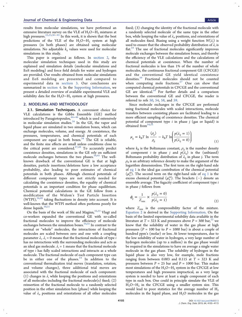
equilibrium for the H2O−H2 mixture defined by the TIP4P/2005-Marx force fields are shown in Figure 4. Raw data areprovided in Table S8. For this mixture, all simulations areperformed in the CFCGE, at T = 323 K, T = 366 K, and T =423 K. It is clear from Figure 4 that the solubilities of water inthe gas phase are significantly underestimated for the wholepressure range. This is mainly due to the fact that the chemicalpotential of TIP4P/2005 water is significantly underpredicted,as shown in Figure 2. Since the predicted water solubilities inthe gas phase are systematically lower for the TIP4P/2005-Marx mixture (see Figures 3a and 4a), the statistics for watersolubilities obtained from CFCGE simulations are worse. Thissampling issue is explained in section 2.1. Similarly, thecomputed isotherms of hydrogen in the liquid phase areslightly underpredicted. For the mixture defined byTIP4P2005-Marx force fields, better agreement with experi-ments is observed for solubilities in the liquid phase for alltemperatures. At T = 366 K, the deviation from experimentaldata is about 14% between P = 50 bar and P = 100 bar. At T =423 K the deviation from experimental data is about 5%between P = 50 bar and P = 80 bar.The solubilities obtained from phase coexistence at

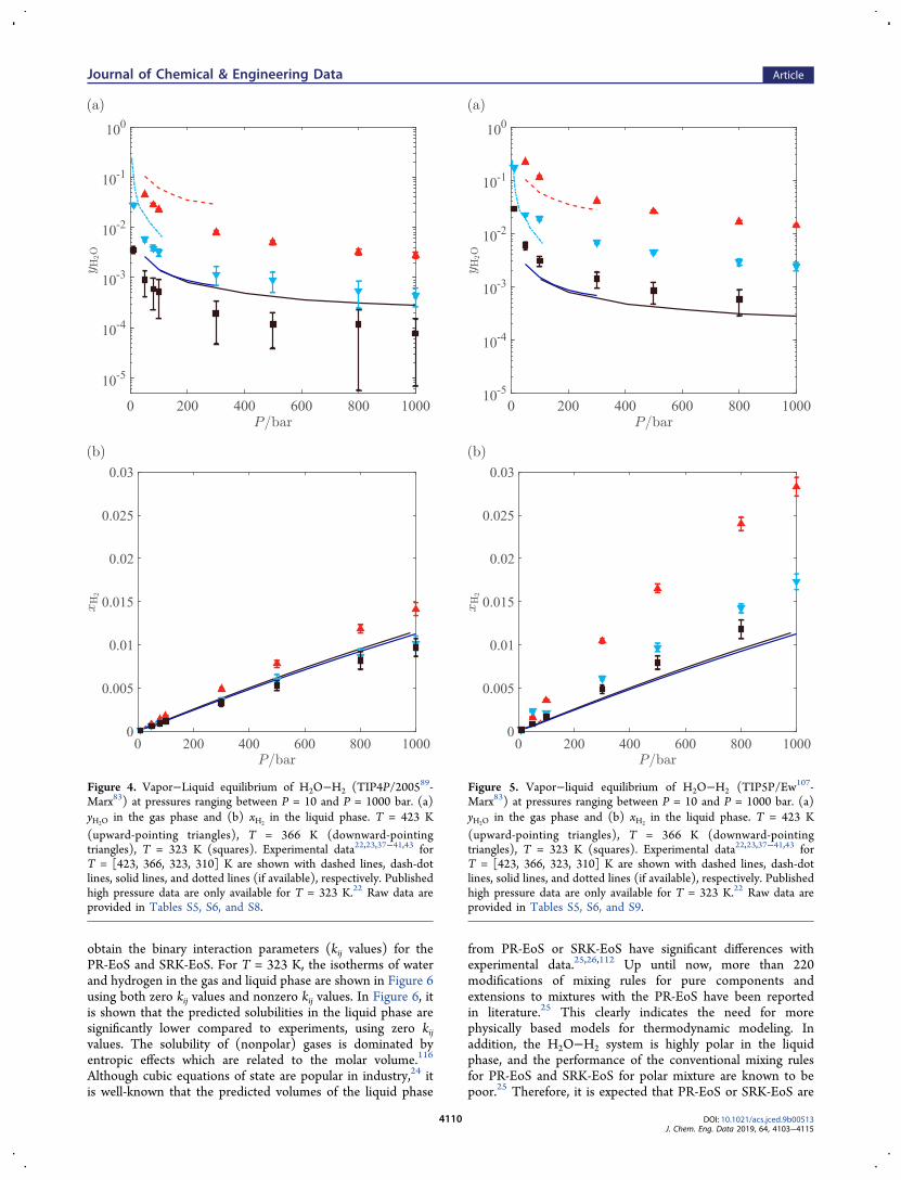
equilibrium for H2O−H2 mixture defined by TIP5P/Ew-Marx force fields are shown in Figure 5. Raw data are providedin Table S9. For this system, all simulations are performed inthe CFCGE, at T = 323 K, T = 366 K, and T = 423 K. In sharpcontrast to the TIP4P/2005-Marx system, both calculatedsolubilities in the liquid and gas using the TIP5P/Ew-Marxsystem are overpredicted. The solubilities of hydrogen in theliquid phase are very similar to those obtained form the TIP3P-Marx force fields. To explain the results in a coherent way, it isimportant to consider the predicted water isotherms in the gasphase in Figures 3 to 5 and the calculated chemical potentialsof pure water in Figure 2b simultaneously. From these figures,it can be concluded that underpredicting the solubilties in thegas phase is directly related to underpredicting the chemicalpotential of water (TIP4P/2005). Similarly, overpredicting thesolubilties of water in the gas phase is directly related tooverpredicting the chemical potential of water (TIP5P/Ew).

3.2. Equation of State Modeling. The water content inthe gas phase and the solubility of hydrogen in the liquid phaseare also calculated using the PR-EoS and SRK-EoS. Highpressure experimental solubilites at T = 323 K were used to

Figure 3. Vapor−liquid equilibrium of H2O−H2 (TIP3P102-Marx83)

at pressures ranging between P = 10 and P = 1000 bar. (a) yH2O in the

gas phase and (b) xH2in the liquid phase. T = 423 K (upward-

pointing triangles), T = 366 K (downward-pointing triangles), T =323 K (squares), T = 310 K (circles), T = 283 (right-pointingtriangles). Experimental data22,23,37−41,43 for T = [423, 366, 323, 310]K are shown with dashed lines, dash-dot lines, solid lines, and dottedlines, respectively. Published high pressure data are only available forT = 323 K.22 Raw data are provided in Tables S5, S6, and S7.

Journal of Chemical & Engineering Data Article

DOI: 10.1021/acs.jced.9b00513J. Chem. Eng. Data 2019, 64, 4103−4115

4109

obtain the binary interaction parameters (kij values) for thePR-EoS and SRK-EoS. For T = 323 K, the isotherms of waterand hydrogen in the gas and liquid phase are shown in Figure 6using both zero kij values and nonzero kij values. In Figure 6, itis shown that the predicted solubilities in the liquid phase aresignificantly lower compared to experiments, using zero kijvalues. The solubility of (nonpolar) gases is dominated byentropic effects which are related to the molar volume.116

Although cubic equations of state are popular in industry,24 itis well-known that the predicted volumes of the liquid phase

from PR-EoS or SRK-EoS have significant differences withexperimental data.25,26,112 Up until now, more than 220modifications of mixing rules for pure components andextensions to mixtures with the PR-EoS have been reportedin literature.25 This clearly indicates the need for morephysically based models for thermodynamic modeling. Inaddition, the H2O−H2 system is highly polar in the liquidphase, and the performance of the conventional mixing rulesfor PR-EoS and SRK-EoS for polar mixture are known to bepoor.25 Therefore, it is expected that PR-EoS or SRK-EoS are

Figure 4. Vapor−Liquid equilibrium of H2O−H2 (TIP4P/200589-Marx83) at pressures ranging between P = 10 and P = 1000 bar. (a)yH2O in the gas phase and (b) xH2

in the liquid phase. T = 423 K(upward-pointing triangles), T = 366 K (downward-pointingtriangles), T = 323 K (squares). Experimental data22,23,37−41,43 forT = [423, 366, 323, 310] K are shown with dashed lines, dash-dotlines, solid lines, and dotted lines (if available), respectively. Publishedhigh pressure data are only available for T = 323 K.22 Raw data areprovided in Tables S5, S6, and S8.

Figure 5. Vapor−liquid equilibrium of H2O−H2 (TIP5P/Ew107-Marx83) at pressures ranging between P = 10 and P = 1000 bar. (a)yH2O in the gas phase and (b) xH2

in the liquid phase. T = 423 K(upward-pointing triangles), T = 366 K (downward-pointingtriangles), T = 323 K (squares). Experimental data22,23,37−41,43 forT = [423, 366, 323, 310] K are shown with dashed lines, dash-dotlines, solid lines, and dotted lines (if available), respectively. Publishedhigh pressure data are only available for T = 323 K.22 Raw data areprovided in Tables S5, S6, and S9.

Journal of Chemical & Engineering Data Article

DOI: 10.1021/acs.jced.9b00513J. Chem. Eng. Data 2019, 64, 4103−4115

4110

not able to predict solubilities of hydrogen in liquid wateraccurately. With the fitted kij values, the obtained solubilities ofhydrogen in the liquid phase are in excellent agreement withexperimental data for p < 400 bar. However, the solubilities inthe gas phase deviate significantly using the fitted kij values.Therefore, calculations of VLE of H2O−H2 mixtures using PR-EoS and SRK-EoS do not yield satisfactory results for bothphases simultaneously, with or without adjusted kij values.

4. CONCLUSIONS

Molecular simulations are used to model the VLE behavior ofH2O−H2 mixtures for pressures between P = 10 bar and P =1000 bar. In Tables S5 and S6, a detailed overview of availableexperimental data has been provided for this system. It isshown that commonly used cubic equations of state, withconventional mixing rules fail to predict the composition of thegas and the liquid phases accurately. For the differentmolecular models for hydrogen, the Buch force field77

(single-site model) and the Marx force field (includingquadrupole moment) predict the density and fugacitycoefficient of hydrogen in good agreement with experimentsup to P = 1000 bar. In this study, no force field for rigid waterwith fixed point charges could accurately predict both thechemical potential and the density of water. The computedchemical potentials of TIP3P water102 have the best agreementwith experimental data from REFPROP75 with a deviation ofca. +50 K (in units of energy/kB) for pressures between P =100 bar and P = 1000 bar. This may be partly due to the factthat one of the target fitting parameters for the TIP3P forcefield is the heat of vaporization, unlike the TIP4P/2005 andTIP5P/Ew force fields. The computed chemical potentials (inunits of energy/kB) of the TIP4P/2005 and TIP5P/Ew deviateon average by −500 K and +250 K from experimental data inthis pressure range, respectively. Both the TIP4P/2005 andTIP5P/Ew force fields can predict the density of liquid waterin good agreement with the experiments for the whole pressurerange. From the simulation results, it is observed thatsolubilities of water in the gas phase are systematicallyunderpredicted when using the TIP4P/2005 force field. Thisforce field also underpredicts the chemical potential of liquidwater compared to experiments. The highest solubilities in thegas phase are predicted using the TIP5P/Ew force field withthe largest values for the calculated chemical potential of water.The best agreement between the predicted gas phasecompositions and experiments for the whole pressure rangeis observed for the TIP3P force field. This suggests that asuitable water force field for studying the VLE of H2O−H2mixtures can be screened based on the chemical potential ofthe water model in the liquid phase. On the basis of thescreening of seven water force fields in this study, it turns outthat the TIP3P and SPC force fields (with very similar valuesfor chemical potential of liquid water) can best predict theequilibrium vapor phase coexistence composition of the H2O−H2 system. For all temperatures in this study, we observed thatthe solubility of water in the gas phase at coexistence issignificantly higher than 5 μmol water per mol hydrogen (asallowed by the ISO standard). Therefore, an additional step forremoving water from the gas phase is required. Despite the factthat the molecular simulations significantly outperform cubicEoS modeling for the VLE of H2O−H2 mixtures, the predictedliquid phase compositions need further improvements. Thesolubilities of hydrogen in the liquid phase are overpredictedusing the TIP3P-Marx and TIP5P/Ew-Marx force fields. Thebest agreement between the calculated liquid phase composi-tion and experiments is observed for the TIP4P/2005-Marxsystem (although the predicted solubilities are slightly lower).Further improvements in simulations of H2O−H2 systems maybe realized taking polarizability of water molecules intoaccount. Therefore, further molecular simulations of theH2O−H2 system are recommended using polarizable force

Figure 6. VLE of H2O−H2 at T = 323 K and pressures rangingbetween P = 100 and P = 1000 bar, obtained from EoS modeling. (a)mole fraction of water in the gas phase, (b) mole fraction of hydrogenin the liquid phase. Experimental solubilities22,23 are shown withcircles. In both subfigures, the results are shown for kij = 0: PR-EoS108

(lines), SRK-EoS109 (dashed lines). The results from the γ−ϕ methodare shown with open symbols: PR-EoS (upward-pointing triangles)and the SRK-EoS (downward-pointing triangles). The results for thefitted BIP for the PR-EoS (kij = −0.89) are shown with dash-dot lines.The results for the fitted BIP for the SRK-EoS (kij = −1.51) are shownwith dotted lines.

Journal of Chemical & Engineering Data Article

DOI: 10.1021/acs.jced.9b00513J. Chem. Eng. Data 2019, 64, 4103−4115

4111

fields for water, especially to improve the predictions for theliquid phase composition.

■ ASSOCIATED CONTENT*S Supporting Information. The Supporting Information is available free of charge on theACS Publications website at DOI: 10.1021/acs.jced.9b00513.

Derivation of eq 2; force field parameters for water andhydrogen; calculated densities and fugacity coefficientsfor pure hydrogen in the gas phase (different forcefields); calculated densities and chemical potentials forpure liquid water (different force fields); experimentalsolubilities of hydrogen and water vapor in the H2O−H2mixture (liquid phase, gas phase, repectively) atcoexistence; compositions of H2O−H2 mixtures atequilibrium using MC simulations; equation of stateparameters for the PR-EoS and SRK-EoS (PDF)

■ AUTHOR INFORMATIONCorresponding Author*E-mail: t.j.h.vlugt@tudelft.nl.ORCIDAhmadreza Rahbari: 0000-0002-6474-3028Mahinder Ramdin: 0000-0002-8476-7035Othonas A. Moultos: 0000-0001-7477-9684Thijs J. H. Vlugt: 0000-0003-3059-8712NotesThe authors declare no competing financial interest.

■ ACKNOWLEDGMENTSThis work was sponsored by NWO Exacte Wetenschappen(Physical Sciences) for the use of supercomputer facilities, withfinancial support from the Nederlandse Organisatie voorWetenschappelijk Onderzoek (Netherlands Organization forScientific Research, NWO). T.J.H.V. acknowledges NWO−CW for a VICI grant.

■ REFERENCES(1) World Population Prospects: The 2017 Revision, Key Findings andAdvance Tables, ESA/P/WP/248. 2017; https://population.un.org/wpp/Publications/Files/WPP2017_KeyFindings.pdf (accessed 17/7/2019).(2) United Nations. Transforming our world: the 2030 Agenda forSustainable Development. (2015) General Assembly Resolution, A/RES/70/1; http://www.un.org/ga/search/view_doc.asp?symbol=A/RES/70/1&Lang=E (accessed 17/7/2019).(3) World Energy Outlook 2018. 2018; www.iea.org/weo (accessed17/7/2019).(4) Adoption of the Paris Agreement, FCCC/CP/2015/L.9/Rev.1.2015; https://unfccc.int/resource/docs/2015/cop21/eng/l09r01.pdf(accessed 17/7/2019).(5) Gallo, A.; Simoes-Moreira, J.; Costa, H.; Santos, M.; Moutinhodos Santos, E. Energy storage in the energy transition context: Atechnology review. Renewable Sustainable Energy Rev. 2016, 65, 800−822.(6) Zakeri, B.; Syri, S. Electrical energy storage systems: Acomparative life cycle cost analysis. Renewable Sustainable EnergyRev. 2015, 42, 569−596.(7) Evans, A.; Strezov, V.; Evans, T. J. Assessment of utility energystorage options for increased renewable energy penetration. RenewableSustainable Energy Rev. 2012, 16, 4141−4147.(8) Mahlia, T.; Saktisahdan, T.; Jannifar, A.; Hasan, M.; Matseelar,H. A review of available methods and development on energy storage;

technology update. Renewable Sustainable Energy Rev. 2014, 33, 532−545.(9) Chen, H.; Cong, T. N.; Yang, W.; Tan, C.; Li, Y.; Ding, Y.Progress in electrical energy storage system: A critical review. Prog.Nat. Sci. 2009, 19, 291−312.(10) Johnston, B.; Mayo, M. C.; Khare, A. Hydrogen: the energysource for the 21st century. Technovation 2005, 25, 569−585.(11) Rahbari, A.; Ramdin, M.; van den Broeke, L. J. P.; Vlugt, T. J.H. Combined steam reforming of methane and formic acid Toproduce syngas with an adjustable H2:CO ratio. Ind. Eng. Chem. Res.2018, 57, 10663−10674.(12) Adolf, J.; Balzer, C.; Louis, J. Energy of the Future? SustainableMobility through Fuel Cells and H2; Shell Deutschland Oil GmbH,2017.(13) Bouwman, P. Electrochemical Hydrogen Compression (EHC)solutions for hydrogen infrastructure. Fuel Cells Bulletin 2014, 2014,12−16.(14) HyET Hydrogen BV; https://hyet.nl/hydrogen (accessed 17/7/2019).(15) Bampaou, M.; Panopoulos, K. D.; Papadopoulos, A. I.; Seferlis,P.; Voutetakis, S. An electrochemical hydrogen compression model.Chem. Eng. Trans. 2018, 70, 1213.(16) Strobel, R.; Oszcipok, M.; Fasil, M.; Rohland, B.; Jorissen, L.;Garche, J. The compression of hydrogen in an electrochemical cellbased on a PE fuel cell design. J. Power Sources 2002, 105, 208−2157th Ulmer Elektrochemische Tage. .(17) Suermann, M.; Kiupel, T.; Schmidt, T. J.; Buchi, F. N.Electrochemical hydrogen compression: efficient pressurizationconcept derived from an energetic evaluation. J. Electrochem. Soc.2017, 164, F1187−F1195.(18) Rohland, B.; Eberle, K.; Strobel, R.; Scholta, J.; Garche, J.Electrochemical hydrogen compressor. Electrochim. Acta 1998, 43,3841−3846.(19) Nordio, M.; Rizzi, F.; Manzolini, G.; Mulder, M.; Raymakers,L.; Van Sint Annaland, M.; Gallucci, F. Experimental and modellingstudy of an electrochemical hydrogen compressor. Chem. Eng. J. 2019,369, 432−442.(20) Casati, C.; Longhi, P.; Zanderighi, L.; Bianchi, F. Somefundamental aspects in electrochemical hydrogen purification/compression. J. Power Sources 2008, 180, 103−113.(21) Hydrogen fuel, Product specification, Part 2: Proton exchangemembrane (PEM) fuel cell applications for road vehicles. InternationalStandard, 2012; Vol. 2012; www.iso.org/committee/54560/x/catalogue/ (accessed 17/7/2019).(22) Bartlett, E. P. The concentration of water vapor in compressedhydrogen, Nitrogen and a mixture of these gases in the presence ofcondensed water. J. Am. Chem. Soc. 1927, 49, 65−78.(23) Wiebe, R.; Gaddy, V. L. The solubility of hydrogen in water at0, 50, 75 and 100° from 25 to 1000 atm. J. Am. Chem. Soc. 1934, 56,76−79.(24) Hendriks, E.; Kontogeorgis, G. M.; Dohrn, R.; de Hemptinne,J.-C.; Economou, I. G.; Zilnik, L. F.; Vesovic, V. Industrialrequirements for thermodynamics and transport properties. Ind.Eng. Chem. Res. 2010, 49, 11131−11141.(25) Lopez-Echeverry, J. S.; Reif-Acherman, S.; Araujo-Lopez, E.Peng-Robinson equation of state: 40 years through cubics. Fluid PhaseEquilib. 2017, 447, 39−71.(26) Iwai, Y.; Margerum, M. R.; Lu, B. C. Y. A new three-parametercubic equation of state for polar fluids and fluid mixtures. Fluid PhaseEquilib. 1988, 42, 21−41.(27) Diamantonis, N. I.; Boulougouris, G. C.; Mansoor, E.;Tsangaris, D. M.; Economou, I. G. Evaluation of cubic, SAFT, andPC-SAFT equations of state for the vapor-liquid equilibriummodeling of CO2 mixtures with other gases. Ind. Eng. Chem. Res.2013, 52, 3933−3942.(28) Kwak, T.; Mansoori, G. A. Van der Waals mixing rules for cubicequations of state. Applications for supercritical fluid extractionmodelling. Chem. Eng. Sci. 1986, 41, 1303−1309.

Journal of Chemical & Engineering Data Article

DOI: 10.1021/acs.jced.9b00513J. Chem. Eng. Data 2019, 64, 4103−4115

4112

(29) Harstad, K. G.; Miller, R. S.; Bellan, J. Efficient high-pressurestate equations. AIChE J. 1997, 43, 1605−1610.(30) Jhaveri, B. S.; Youngren, G. K. Three-parameter modification ofthe Peng-Robinson equation of state to improve volumetricpredictions. SPE Reservoir Eng. 1988, 3, 1033−1040.(31) Poling, B. E.; Prausnitz, J. M.; O’Connell, J. P. The properties ofgases and liquids, 5th ed.; McGraw-Hill New York: New York, USA,2001.(32) Valderrama, J. O. The State of the Cubic Equations of State.Ind. Eng. Chem. Res. 2003, 42, 1603−1618.(33) Gross, J.; Sadowski, G. Perturbed-Chain SAFT: An equation ofstate based on a perturbation theory for chain molecules. Ind. Eng.Chem. Res. 2001, 40, 1244−1260.(34) Frenkel, D.; Smit, B. Understanding molecular simulation: fromalgorithms to applications, 2nd ed.; Academic Press: San Diego, CA,2002.(35) Sun, R.; Lai, S.; Dubessy, J. Calculations of vapor-liquidequilibria of the H2O-N2 and H2O-H2 systems with improved SAFT-LJ EOS. Fluid Phase Equilib. 2015, 390, 23−33.(36) Meyer, M.; Tebbe, U.; Piiper, J. Solubility of inert gases in dogblood and skeletal muscle. Pfluegers Arch. 1980, 384, 131−134.(37) Gillespie, P. C.; Wilson, G. M. Vapor-Liquid Equilibrium Dataon Water-Substitue Gas Components; Gas Processors Association,1980; pp RR_41, pp 1−34; https://www.osti.gov/biblio/6782591(accessed 17/7/2019).(38) Kling, G.; Maurer, G. The solubility of hydrogen in water andin 2-aminoethanol at temperatures between 323 and 423 K andpressures up to 16 M Pa. J. Chem. Thermodyn. 1991, 23, 531−541.(39) Devaney, W.; Berryman, J. M.; Kao, P.-L.; Eakin, B. HighTemperature V-L-E Measurements for Substitute Gas Components; GasProcessors Association, 1978; pp 1−27.(40) Jung, J. Loslichkeit von Kohlenmonoxid und Wasserstoff inWasser zwisen 0 C und 300 C. Ph.D. Thesis, RWTH Aachen, 1962.(41) Ipatev, V.; Teodorovich, V. Equilibrium compositions of vapor-gas mixtures over solutions. Zh. Obshch. Khim. 1934, 4, 395−399.(42) Ugrozov, V. V. Equilibrium compositions of vapor-gas mixturesover solutions. Russ. J. Phys. Chem. 1996, 70, 1240−1241.(43) Maslennikova, V. Y.; Goryunova, N.; Subbotina, L.; Tsiklis, D.The solubility of water in compressed hydrogen. Russ. J. Phys. Chem.1976, 50, 240−243.(44) Panagiotopoulos, A. Z. Molecular simulation of phaseequilibria: simple, ionic and polymeric fluids. Fluid Phase Equilib.1992, 76, 97−112.(45) Panagiotopoulos, A. Z. Direct determination of fluid-Phaseequilibria by simulation in the Gibbs ensemble - a Review. Mol. Simul.1992, 9, 1−23.(46) Panagiotopoulos, A. Z. Direct determination of phasecoexistence properties of fluids by Monte Carlo simulation in a newensemble. Mol. Phys. 1987, 61, 813−826.(47) Recht, J.; Panagiotopoulos, A. Z. Finite-size effects andapproach to criticality in Gibbs ensemble simulations. Mol. Phys.1993, 80, 843−852.(48) Siepmann, J. I.; McDonald, I. R.; Frenkel, D. Finite-sizecorrections to the chemical potential. J. Phys.: Condens. Matter 1992,4, 679.(49) Smit, B.; Frenkel, D. Calculation of the chemical potential inthe Gibbs ensemble. Mol. Phys. 1989, 68, 951−958.(50) Rahbari, A.; Poursaeidesfahani, A.; Torres-Knoop, A.;Dubbeldam, D.; Vlugt, T. J. H. Chemical potentials of water,methanol, carbon dioxide and hydrogen sulphide at low temperaturesusing continuous fractional component Gibbs ensemble Monte Carlo.Mol. Simul. 2018, 44, 405−414.(51) Coskuner, O.; Deiters, U. K. Hydrophobic interactions byMonte Carlo simulations. Z. Phys. Chem. 2006, 220, 349−369.(52) Shi, W.; Maginn, E. J. Continuous Fractional ComponentMonte Carlo: an adaptive biasing method for open system atomisticsimulations. J. Chem. Theory Comput. 2007, 3, 1451−1463.(53) Shi, W.; Maginn, E. J. Improvement in molecule exchangeefficiency in Gibbs ensemble Monte Carlo: development and

implementation of the continuous fractional component move. J.Comput. Chem. 2008, 29, 2520−2530.(54) Poursaeidesfahani, A.; Torres-Knoop, A.; Dubbeldam, D.;Vlugt, T. J. H. Direct free energy calculation in the ContinuousFractional Component Gibbs ensemble. J. Chem. Theory Comput.2016, 12, 1481−1490.(55) Poursaeidesfahani, A.; Hens, R.; Rahbari, A.; Ramdin, M.;Dubbeldam, D.; Vlugt, T. J. H. Efficient application of ContinuousFractional Component Monte Carlo in the reaction ensemble. J.Chem. Theory Comput. 2017, 13, 4452−4466.(56) Rahbari, A.; Hens, R.; Dubbeldam, D.; Vlugt, T. J. H.Improving the accuracy of computing chemical potentials in CFCMCsimulations. Mol. Phys. 2019,(57) Poursaeidesfahani, A.; Rahbari, A.; Torres-Knoop, A.;Dubbeldam, D.; Vlugt, T. J. H. Computation of thermodynamicproperties in the continuous fractional component Monte CarloGibbs ensemble. Mol. Simul. 2017, 43, 189−195.(58) Rahbari, A.; Hens, R.; Nikolaidis, I. K.; Poursaeidesfahani, A.;Ramdin, M.; Economou, I. G.; Moultos, O. A.; Dubbeldam, D.; Vlugt,T. J. H. Computation of partial molar properties using continuousfractional component Monte Carlo. Mol. Phys. 2018, 116, 3331−3344.(59) Torres-Knoop, A.; Burtch, N. C.; Poursaeidesfahani, A.; Balaji,S. P.; Kools, R.; Smit, F. X.; Walton, K. S.; Vlugt, T. J. H.; Dubbeldam,D. Optimization of Particle Transfers in the Gibbs Ensemble forSystems with Strong and Directional Interactions Using CBMC,CFCMC, and CB/CFCMC. J. Phys. Chem. C 2016, 120, 9148−9159.(60) Rahbari, A.; Hens, R.; Jamali, S. H.; Ramdin, M.; Dubbeldam,D.; Vlugt, T. J. H. Effect of truncating electrostatic interactions onpredicting thermodynamic properties of water-methanol systems. Mol.Simul. 2019, 45, 336−350.(61) Dubbeldam, D.; Calero, S.; Ellis, D. E.; Snurr, R. Q. RASPA:molecular simulation software for adsorption and diffusion in flexiblenanoporous materials. Mol. Simul. 2016, 42, 81−101.(62) Dubbeldam, D.; Torres-Knoop, A.; Walton, K. S. On the innerworkings of Monte Carlo codes. Mol. Simul. 2013, 39, 1253−1292.(63) Allen, M. P.; Tildesley, D. J. Computer simulation of liquids, 2nded.; Oxford University Press: Oxford, United Kingdom, 2017.(64) Klimovich, P. V.; Shirts, M. R.; Mobley, D. L. Guidelines for theanalysis of free energy calculations. J. Comput.-Aided Mol. Des. 2015,29, 397−411.(65) Naden, L. N.; Pham, T. T.; Shirts, M. R. Linear basis functionapproach to efficient alchemical free energy calculations. 1. Removalof uncharged atomic sites. J. Chem. Theory Comput. 2014, 10, 1128−1149.(66) Naden, L. N.; Shirts, M. R. Linear basis function approach toefficient alchemical free energy calculations. 2. Inserting and deletingparticles with Coulombic interactions. J. Chem. Theory Comput. 2015,11, 2536−2549.(67) Shirts, M. R.; Pande, V. S. Solvation free energies of amino acidside chain analogs for common molecular mechanics water models. J.Chem. Phys. 2005, 122, 134508.(68) Shirts, M. R.; Pitera, J. W.; Swope, W. C.; Pande, V. S.Extremely precise free energy calculations of amino acid side chainanalogs: Comparison of common molecular mechanics force fields forproteins. J. Chem. Phys. 2003, 119, 5740−5761.(69) Shirts, M. R.; Mobley, D. L.; Chodera, J. D. In Annual Reportsin Computational Chemistry; Spellmeyer, D., Wheeler, R., Eds.;Elsevier: United States, 2007; pp 41−59.(70) Deeg, K. S.; Gutierrez-Sevillano, J. J.; Bueno-Perez, R.; Parra, J.B.; Ania, C. O.; Doblare, M.; Calero, S. Insights on the MolecularMechanisms of Hydrogen Adsorption in Zeolites. J. Phys. Chem. C2013, 117, 14374−14380.(71) Sese, L. M. Study of the Feynman-Hibbs effective potentialagainst the path-integral formalism for Monte Carlo simulations ofquantum many-body Lennard-Jones systems. Mol. Phys. 1994, 81,1297−1312.

Journal of Chemical & Engineering Data Article

DOI: 10.1021/acs.jced.9b00513J. Chem. Eng. Data 2019, 64, 4103−4115

4113

(72) Sese, L. M. Feynman-Hibbs potentials and path integrals forquantum Lennard-Jones systems: Theory and Monte Carlosimulations. Mol. Phys. 1995, 85, 931−947.(73) Izadi, S.; Anandakrishnan, R.; Onufriev, A. V. Building WaterModels: a different approach. J. Phys. Chem. Lett. 2014, 5, 3863−3871.(74) Vega, C.; Abascal, J. L. F.; Conde, M. M.; Aragones, J. L. Whatice can teach us about water interactions: a critical comparison of theperformance of different water models. Faraday Discuss. 2009, 141,251−276.(75) Lemmon, E. W.; Span, R. Short fundamental equations of statefor 20 industrial fluids. J. Chem. Eng. Data 2006, 51, 785−850.(76) Lemmon, E. W.; Huber, M. L.; McLinden, M. O. NISTreference fluid thermodynamic and transport properties−REFPROP.NIST standard reference database 2002, 23, v7.(77) Buch, V. Path integral simulations of mixed para-D2 and ortho-D2 clusters: The orientational effects. J. Chem. Phys. 1994, 100, 7610−7629.(78) Hirschfelder, C.; Curtiss, F.; Bird, R. B. Molecular Theory ofGases and Liquids; Wiley: New York, 1954.(79) Koster, A.; Thol, M.; Vrabec, J. Molecular Models for theHydrogen Age: Hydrogen, Nitrogen, Oxygen, Argon, and Water. J.Chem. Eng. Data 2018, 63, 305−320.(80) Cracknell, R. F. Molecular simulation of hydrogen adsorptionin graphitic nanofibres. Phys. Chem. Chem. Phys. 2001, 3, 2091−2097.(81) Belof, J. L.; Stern, A. C.; Space, B. An accurate and transferableintermolecular diatomic hydrogen potential for condensed phasesimulation. J. Chem. Theory Comput. 2008, 4, 1332−1337.(82) Forrest, K. A.; Pham, T.; McLaughlin, K.; Belof, J. L.; Stern, A.C.; Zaworotko, M. J.; Space, B. Simulation of the mechanism of gassorption in a metal-organic framework with open metal sites:molecular hydrogen in PCN-61. J. Phys. Chem. C 2012, 116,15538−15549.(83) Marx, D.; Nielaba, P. Path-integral Monte Carlo techniques forrotational motion in two dimensions: Quenched, annealed, and no-spin quantum-statistical averages. Phys. Rev. A: At., Mol., Opt. Phys.1992, 45, 8968−8971.(84) Camp, J.; Stavila, V.; Allendorf, M. D.; Prendergast, D.;Haranczyk, M. Critical factors in computational characterization ofhydrogen storage in metal-organic frameworks. J. Phys. Chem. C 2018,122, 18957−18967.(85) Yang, Q.; Zhong, C. Molecular simulation of carbon dioxide/methane/hydrogen mixture adsorption in metal-organic frameworks.J. Phys. Chem. B 2006, 110, 17776−17783.(86) Darkrim, F.; Levesque, D. Monte Carlo simulations ofhydrogen adsorption in single-walled carbon nanotubes. J. Chem.Phys. 1998, 109, 4981−4984.(87) Wagner, W.; Pruß, A. The IAPWS formulation 1995 for thethermodynamic properties of ordinary water substance for generaland scientific use. J. Phys. Chem. Ref. Data 2002, 31, 387−535.(88) Vega, C.; Abascal, J. L. F. Simulating water with rigid non-polarizable models: a general perspective. Phys. Chem. Chem. Phys.2011, 13, 19663−19688.(89) Abascal, J. L. F.; Vega, C. A general purpose model for thecondensed phases of water: TIP4P/2005. J. Chem. Phys. 2005, 123,234505.(90) Tsimpanogiannis, I. N.; Moultos, O. A.; Franco, L. F. M.; de M.Spera, M. B.; Erdos, M.; Economou, I. G. Self-diffusion coefficient ofbulk and confined water: a critical review of classical molecularsimulation studies. Mol. Simul. 2019, 45, 425−453.(91) Vega, C. Water: one molecule, two surfaces, one mistake. Mol.Phys. 2015, 113, 1145−1163.(92) Bauer, B. A.; Patel, S. Properties of water along the liquid-vaporcoexistence curve via molecular dynamics simulations using thepolarizable TIP4P-QDP-LJ water model. J. Chem. Phys. 2009, 131,No. 084709.(93) Jiang, H.; Moultos, O. A.; Economou, I. G.; Panagiotopoulos,A. Z. Hydrogen-bonding polarizable intermolecular potential modelfor water. J. Phys. Chem. B 2016, 120, 12358−12370.

(94) Chen, B.; Xing, J.; Siepmann, J. I. Development of polarizablewater force fields for phase equilibrium calculations. J. Phys. Chem. B2000, 104, 2391−2401.(95) Yesylevskyy, S. O.; Schafer, L. V.; Sengupta, D.; Marrink, S. J.Polarizable Water Model for the Coarse-Grained MARTINI ForceField. PLoS Comput. Biol. 2010, 6, 1−17.(96) Gladich, I.; Roeselova, M. Comparison of selected polarizableand nonpolarizable water models in molecular dynamics simulationsof ice Ih. Phys. Chem. Chem. Phys. 2012, 14, 11371−11385.(97) Kunz, A.-P. E.; van Gunsteren, W. F. Development of anonlinear classical polarization model for liquid water and aqueoussolutions: COS/D. J. Phys. Chem. A 2009, 113, 11570−11579.(98) Lamoureux, G.; MacKerell, A. D.; Roux, B. A simple polarizablemodel of water based on classical Drude oscillators. J. Chem. Phys.2003, 119, 5185−5197.(99) Lamoureux, G.; Harder, E.; Vorobyov, I. V.; Roux, B.;MacKerell, A. D. A polarizable model of water for molecular dynamicssimulations of biomolecules. Chem. Phys. Lett. 2006, 418, 245−249.(100) Ren, P.; Ponder, J. W. Polarizable atomic multipole watermodel for molecular mechanics simulation. J. Phys. Chem. B 2003,107, 5933−5947.(101) Laury, M. L.; Wang, L.-P.; Pande, V. S.; Head-Gordon, T.;Ponder, J. W. Revised parameters for the AMOEBA polarizableatomic multipole water model. J. Phys. Chem. B 2015, 119, 9423−9437.(102) Jorgensen, W. L.; Chandrasekhar, J.; Madura, J. D.; Impey, R.W.; Klein, M. L. Comparison of simple potential functions forsimulating liquid water. J. Chem. Phys. 1983, 79, 926−935.(103) Jorgensen, W. L.; Chandrasekhar, J.; Madura, J. D.; Impey, R.W.; Klein, M. L. Comparison of simple potential functions forsimulating liquid water. J. Chem. Phys. 1983, 79, 926−935.(104) Mark, P.; Nilsson, L. Structure and dynamics of the TIP3P,SPC, and SPC/E water models at 298 K. J. Phys. Chem. A 2001, 105,9954−9960.(105) Berendsen, H. J. C.; Grigera, J. R.; Straatsma, T. P. Themissing term in effective pair potentials. J. Phys. Chem. 1987, 91,6269−6271.(106) Horn, H. W.; Swope, W. C.; Pitera, J. W.; Madura, J. D.; Dick,T. J.; Hura, G. L.; Head-Gordon, T. Development of an improvedfour-site water model for biomolecular simulations: TIP4P-Ew. J.Chem. Phys. 2004, 120, 9665−9678.(107) Rick, S. W. A reoptimization of the five-site water potential(TIP5P) for use with Ewald sums. J. Chem. Phys. 2004, 120, 6085−6093.(108) Peng, D.-Y.; Robinson, D. B. A new two-constant equation ofstate. Ind. Eng. Chem. Fundam. 1976, 15, 59−64.(109) Soave, G. Equilibrium constants from a modified Redlich-Kwong equation of state. Chem. Eng. Sci. 1972, 27, 1197−1203.(110) Twu, C. H.; Coon, J. E.; Bluck, D. Comparison of the Peng-Robinson and Soave- Redlich-Kwong equations of state using a newzero-pressure-based mixing Rule for the prediction of high-pressureand high-temperature phase equilibria. Ind. Eng. Chem. Res. 1998, 37,1580−1585.(111) Peneloux, A.; Rauzy, E.; Freze, R. A consistent correction forRedlich-Kwong-Soave volumes. Fluid Phase Equilib. 1982, 8, 7−23.(112) Lin, C.-T.; Daubert, T. E. Estimation of partial molar volumeand fugacity coefficient of components in mixtures from the soave andPeng-Robinson equations of state. Ind. Eng. Chem. Process Des. Dev.1980, 19, 51−59.(113) Leachman, J. W.; Jacobsen, R. T.; Penoncello, S.; Lemmon, E.W. Fundamental equations of state for parahydrogen, normalhydrogen, and orthohydrogen. J. Phys. Chem. Ref. Data 2009, 38,721−748.(114) Horn, H. W.; Swope, W. C.; Pitera, J. W.; Madura, J. D.; Dick,T. J.; Hura, G. L.; Head-Gordon, T. Development of an improvedfour-site water model for biomolecular simulations: TIP4P-EW. J.Chem. Phys. 2004, 120, 9665−9678.(115) Mahoney, M. W.; Jorgensen, W. L. A five-site model for liquidwater and the reproduction of the density anomaly by rigid,

Journal of Chemical & Engineering Data Article

DOI: 10.1021/acs.jced.9b00513J. Chem. Eng. Data 2019, 64, 4103−4115

4114

nonpolarizable potential functions. J. Chem. Phys. 2000, 112, 8910−8922.(116) Wilhelm, E.; Waghorne, E.; Hefter, G.; Hummel, W.; Maurer,G.; Rebelo, L. P. N.; da Ponte, M. N.; Battino, R.; Clever, L.; vanHook, A.; Domanska-Zelazna, U.; Tomkins, R. P. T.; Richon, D.; deStafani, V.; Coquelet, C.; Costa Gomes, M.; Siepmann, J. I.;Anderson, K. E.; Eckert, F.; Grolier, J.-P.; Boyer, S.; Salminen, J.;Dohrn, R.; Leiberich, R.; Fele Zilnik, L.; Fages, J.; Macedo, M. E.;Gmehling, J.; Brennecke, J.; Cordes, W.; Prausnitz, J.; Goodwin, A. R.;Marsh, K.; Peters, C. J.; Voigt, W.; Koenigsberger, E.; May, P.; Kamps,A. P.-S.; Shariati, A.; Raeissi, S.; Padua, A. A. H.; Sauceau, M.; Pinho,S. P. P.; Kaskiala, T.; Kobylin, P. In Developments and Applications inSolubility; Letcher, T. M., Ed.; The Royal Society of Chemistry, 2007.

Journal of Chemical & Engineering Data Article

DOI: 10.1021/acs.jced.9b00513J. Chem. Eng. Data 2019, 64, 4103−4115

4115