soil parameters which can be determined with seismic

SOIL PARAMETERS wHICH CAN BE DETERMINED

wITH SEISMIC VELOCITIES

Sismik Hızlar İle Saptanabilen Zemin Parametreleri

Ali KEÇELİ

Salacak Mh., B.Selattin Pınar Sk. No:130/8, Üsküdar, İstanbul, TURKEY (keceliali_jfz@ yahoo.com.tr)

ABSTRACT

The determination of seismic velocities, elasticity modulus and structural properties of soils is not enough in the design of engineering projects. Therefore, an ultimate bearing capacity has been defined by expressing the earth pressure with the seismic shear wave velocity. In this context, a density relation has also been defined in terms of the seismic shear wave. Utilising of similarity of safety factor and [Vp/Vs], velocity ratio values, it has been shown that the V

p /V

s velocity ratio can be used

together with safety factor and water reduction factor. The allowable bearing capacity values obtained are in agreement with the building code for the allowable bearing capacity values. It was shown that the allowable bearing capacity including spread footing shape could be defined similarly to that of the Meyerhof’s relation for SPT (N). The allowable bearing capacity values obtained for the spread footing were in agreement with the values given by Brown. The elastic settlement and the subgrade reaction coefficient have also been determined from Boussinesq’s equation. It was observed that the load-settlement curve obtained indicates similar variation to that in the soil mechanics. The subgrade reaction values obtained were in agreement with the Bowles’s experimental values. While the underground properties are elucidated by seismic method, it is also possible to obtain a reliable knowledge about the allowable bearing capacity, settlement and subgrade reaction values quickly and low cost by this technique proposed here.

Key words: Allowable bearing capacity, load-settlement curve, subgrade reaction coefficient, seismic velocity.

ÖZET

Sismik hızların, elastisite modüllerinin ve zeminlerin yapısal özelliklerinin saptanması mühendislik projelerinin tasarımında yeterli olmamaktadır. Bu nedenle, Sismik kayma dalga empedansı ile yer basıncı ifade edilerek zeminlerin nihai taşıma kapasitesi tanımlanmıştır. Bu

bağlamda, kayma dalgası hızına bağlı yoğunluk tanımı yapılmıştır. Güvenlik faktörü ile [Vp/Vs] hız oranı değerlerinin benzerliğinden yararlanarak, [Vp/Vs]’nın güvenlik faktörü ve yer altı suyu indirgeme faktörü olarak kullanılabileceği gösterilmiştir. Elde edilen müsaade edilebilir taşıma kapasitesi değerleri standart tablo verileri ile uyum içinde olduğu gösterilmiştir. Tekil temel (somel) için müsaade edilebilir taşıma kapasitesi Meyehof’un SPT(N) tanımına benzer olarak tanımlanabileceği gösterilmiştir. Tekil temel için elde edilen müsaade edilebilir taşıma kapasitesi değerleri Brown tarafından verilenler ile uyum içinde olmuştur. Ayrıca, Boussinesq denkleminden zemin oturması ve yatak katsayısı saptanabilmiştir. Yük-oturma eğrisi zemin mekaniğindekine benzer değişim göstermiştir. Sismik hızlarla yapısal jeoloji ve diğer özellikler aydınlatılırken, müsaade edilebilir taşıma kapasitesi, zemin oturması ve yatak katsayısı değerleri hakkında daha çabuk ve ucuz olarak güvenilir ön bilgi elde etmek mümkün olmaktadır.

1. INTRODUCTION

The determinaton of seismic velocities, elasticity modulus and structural properties of soils is not enough in the design of engineering projects. In the design of engineering structures one of the main factors related to soil is bearing capacity and other is settlement so that is subgrade reaction.

Many investigators have extensively studied to obtain a relation between the various parameters of soil mechanics and the seismic wave velocities. Some of them: (Hardin et al. 1968; Hardin et al. 1972; Imai et al. 1976; Ohkubo et al. 1976; Othman 2005; Uyanık, O. 2010, 2011; Seed, et al. 1984 and others). Also, many investigators have extensively studied to obtain a relation between various litological properties of rocks and the seismic wave velocities for the aim of exploration geophysics. Some of them: (Guliev 2007; Hicks, 2006; Jongmans 1992; Philips et al. 1989; Stuempel et al. 1984; Tatham 1982; Wang, 2001; and others).

doi: 11.a02/jeofizik-1011-31Jeofizik, 2012, 16, 17-29

c 2012 TMMOB Jeofizik Mühendisleri Odası

A. Keçeli

c 2012 TMMOB Jeofizik Mühendisleri Odası, Jeofizik, 2012, 16, 17-29

18

Few authors have published an empirical formula between seismic wave velocities and Standart Penetration Test (SPT) N- blow counts for the determination of bearing capacity, (Imai et al. 1972; Imai 1975; Parry 1977; Sternberg et al. 1990).

(Keçeli 1990, 2000) showed that the determination of the presumptive or allowable bearing capacity could be obtained by means of the Seismic Method. (Tezcan et al. 2009, 2011; Kaplan et al. 2011, fig.1) has defined an allowable bearing capacity (q

a) and a settlement as

depending on the layer thickness. But, it is well known that the soil bearing capacity, settlement and (E) elasticity modulus cannot be dependent on the layer thickness. Nevertheless, they obtained also an allowable bearing capacity by changing the notation of the relations in the article of (Keçeli 2000).

The elasticity theory is often used for elastic or instantaneous settlement, although it gives approximate value. In soil deformations studies, shear modulus and elasticity modulus are very important. The analysis of geotechnical engineering problems requires characterization of dynamic soil properties using seismic velocities. Therefore, shear wave velocity (Vs) is the most commonly used to measure the parameter of soil characterization. Starting from this point of view, in this paper, relationships between shear wave impedance and allowable bearing capacity for spread foundation, settlement, subgrade reaction coefficient were investigated by using seismic shear wave velocities.

2. OBTAINING ULTIMATE BEARING CAPACITY

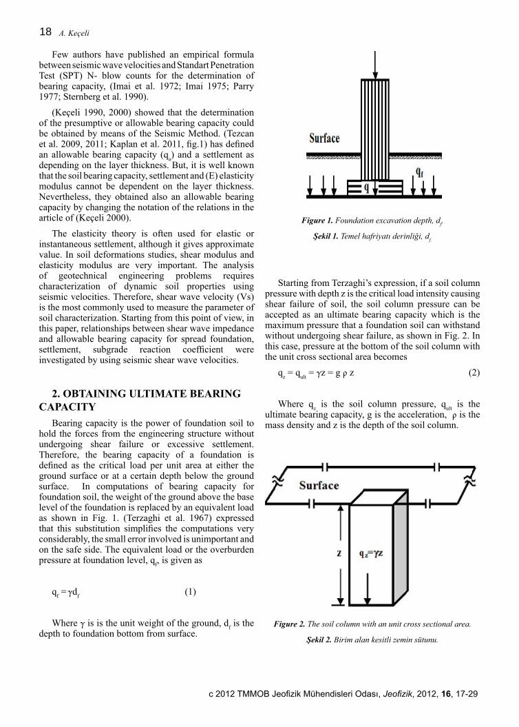
Bearing capacity is the power of foundation soil to hold the forces from the engineering structure without undergoing shear failure or excessive settlement. Therefore, the bearing capacity of a foundation is defined as the critical load per unit area at either the ground surface or at a certain depth below the ground surface. In computations of bearing capacity for foundation soil, the weight of the ground above the base level of the foundation is replaced by an equivalent load as shown in Fig. 1. (Terzaghi et al. 1967) expressed that this substitution simplifies the computations very considerably, the small error involved is unimportant and on the safe side. The equivalent load or the overburden pressure at foundation level, q

f, is given as

qf =

γd

f (1)

Where γ is is the unit weight of the ground, df is the

depth to foundation bottom from surface.

Figure 1. Foundation excavation depth, df.

Şekil 1. Temel hafriyatı derinliği, df.

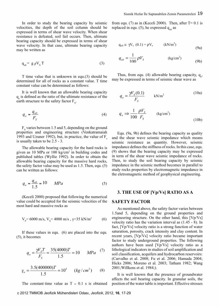
Starting from Terzaghi’s expression, if a soil column pressure with depth z is the critical load intensity causing shear failure of soil, the soil column pressure can be accepted as an ultimate bearing capacity which is the maximum pressure that a foundation soil can withstand without undergoing shear failure, as shown in Fig. 2. In this case, pressure at the bottom of the soil column with the unit cross sectional area becomes

qz = q

ult = γz = g ρ z (2)

Where qz is the soil column pressure, q

ult is the

ultimate bearing capacity, g is the acceleration, ρ is the mass density and z is the depth of the soil column.

Figure 2. The soil column with an unit cross sectional area.

Şekil 2. Birim alan kesitli zemin sütunu.



19

In order to study the bearing capacity by seismic velocities, the depth of the soil column should be expressed in terms of shear wave velocity. When shear resistance is defeated, soil fail occurs. Then, ultimate bearing capacity should be expressed in terms of shear wave velocity. In that case, ultimate bearing capacity may be written as

qult

= g ρVS T (3)

T time value that is unknown in equ.(3) should be determined for all of rocks as a constant value. T time constant value can be determined as follows:

It is well known that an allowable bearing capacity q

a is defined as the ratio of the ultimate resistance of the

earth structure to the safety factor FS.

S

ulta F

qq = (4)

FS varies between 1.5 and 5, depending on the ground

properties and engineering structure (Venkatramaiah 1993 and Uzuner 1992), but, in practice, the value of F

s

is usually taken to be 2.5 - 3.

The allowable bearing capacity for the hard rocks is given as 10 MPa or 100 kg/cm2 in building codes and published tables (Wyllie 1992). In order to obtain the allowable bearing capacity for the massive hard rocks, the safety factor value may be used as 1.5. Then, equ. (5) can be written as follows:

MPaq

q ulta 10

5.1== (5)

(Keceli 2000) proposed that following the numerical value could be accepted for the seismic velocities of the most hard and massive rocks as

VP= 6000 m/s, V

S= 4000 m/s , γ=35 kN/m3 (6)

If these values in equ. (6) are placed into the equ. (5), it becomes

(7)

(8)

6

MPaT

F

TVq

S

Sa 10

5.1

)4000(35===

! (7)

or )/(105.1

)400000(5.3 25 cmkgT

qa == (8)

The constant time value as T # 0.1 s is obtained from equ. (7) as in (Keceli 2000). Then, after T= 0.1 is replaced

in equ. (5), he expressed qult as

qult # !Vs (0.1) = "Vs (kN/m2) (9a)

or Sult Vq !100

1= (kg/cm

2) (9b)

Thus, from equ. (4) allowable bearing capacity, qa, may be expressed in terms of seismic shear wave as

S

Sa

F

Vq

)1.0(!= kN/m

2 (10a)

or

S

Sa

F

Vq

!

100

1" (kg/cm

2) (10b)

Equ. (9a, 9b) defines the bearing capacity as quality and the shear wave seismic impedance which means seismic

resistance as quantity. However, seismic impedance defines the stiffness of rocks. In this case, equ. (9) shows

that the bearing capacity may be expressed in term of the shear wave seismic impedance of rocks. Then, to study

the soil bearing capacity by seismic impedance in the seismic method becomes in parallel to study rocks

properties by electromagnetic impedance in the eletromagnetic method of geophysical engineering.

3. THE USE OF [Vp/Vs] RATIO AS A SAFETY FACTOR

As mentioned above, the safety factor varies between 1.5and 5, depending on the ground properties and

engineering structure. On the other hand, this [Vp/Vs] velocity ratio has the variation interval as (1.45 - 8). In

fact, [Vp/Vs] velocity ratio is a strong function of water saturation, porosity, crack intensity and clay content. In

recent years, [Vp/Vs] velocity ratio became important factor to study underground properties. The following

The constant time value as T = 0.1 s is obtained

from equ. (7) as in (Keceli 2000). Then, after T= 0.1 is replaced in equ. (5), he expressed q

ult as

(9a)

6

MPaT

F

TVq

S

Sa 10

5.1

)4000(35===

! (7)

or )/(105.1

)400000(5.3 25 cmkgT

qa == (8)



qult # !Vs (0.1) = "Vs (kN/m2) (9a)

or Sult Vq !100

1= (kg/cm

2) (9b)


S

Sa

F

Vq

)1.0(!= kN/m

2 (10a)

or

S

Sa

F

Vq

!

100

1" (kg/cm

2) (10b)











(9b)

Thus, from equ. (4) allowable bearing capacity, qa,

may be expressed in terms of seismic shear wave as

(10a)

6

MPaT

F

TVq

S

Sa 10

5.1

)4000(35===

! (7)

or )/(105.1

)400000(5.3 25 cmkgT

qa == (8)



qult # !Vs (0.1) = "Vs (kN/m2) (9a)

or Sult Vq !100

1= (kg/cm

2) (9b)


S

Sa

F

Vq

)1.0(!= kN/m

2 (10a)

or

S

Sa

F

Vq

!

100

1" (kg/cm

2) (10b)











(10b)

Equ. (9a, 9b) defines the bearing capacity as quality and the shear wave seismic impedance which means seismic resistance as quantity. However, seismic impedance defines the stiffness of rocks. In this case, equ. (9) shows that the bearing capacity may be expressed in term of the shear wave seismic impedance of rocks. Then, to study the soil bearing capacity by seismic impedance in the seismic method becomes in parallel to study rocks properties by electromagnetic impedance in the eletromagnetic method of geophysical engineering.

3. THE USE OF [Vp/Vs] RATIO AS A

SAFETY FACTOR

As mentioned above, the safety factor varies between 1.5and 5, depending on the ground properties and engineering structure. On the other hand, this [Vp/Vs] velocity ratio has the variation interval as (1.45 - 8). In fact, [Vp/Vs] velocity ratio is a strong function of water saturation, porosity, crack intensity and clay content. In recent years, [Vp/Vs] velocity ratio became important factor to study underground properties. The following authors have been used [Vp/Vs] velocity ratio as a lithological indicators in studies of soil amplification and soil classification, acquifers and hydrocarbon reservoirs: (Carvalho et al. 2008; Fu et al. 2006; Hamada 2004; Hicks 2006; Moreno et al. 2003; Tatham 1982; Wang 2001;Willkens et al. 1984;).

It is well known that the presence of groundwater affects the soil bearing capacity. In granular soils, the position of the water table is important. Effective stresses

10

A. Keçeli


20

in saturated sands can be as much as 50% lower than in dry sand. Seismic wave velocities are also affected from the groundwater. The water saturation in the granular soil causes compressional wave velocity to increase and shear wave velocity to decrease. As a result, [V

p /V

s]

velocity ratio increases depending on the water saturation in granular soil. In practice, the safety coefficient value is generally used as 3 for the saturated granular soil. Also, the [V

p /V

s] velocity ratio value to be obtained for the

same saturated granular soil equals nearly to 6. So that, the value of [V

p /V

s] ratio will become approximately

two times of FS.

Therefore, there is no need to reduce bearing capacity as in soil mechanics when [V

p /V

s]

velocity ratio is used as a safety factor in the soil studies. When F

S and [V

p /V

s] are used together in soil studies,

the more reliable results may be achieved. Consequently, the use of [V

p /V

s] as safety factor provides a reliable

choices of FS.

The values of [Vp /V

s] and F

S depending properties

of soils and rocks increase from loose soil to hard rock. Classifying of this variation type may be arranged as shown in Table 1.

Table 1. The similarity between the values of safety factor and [Vp/Vs] velocity ratio.

Soil and rock type VP

VS

( Vp / V

s ) Safety factor (F

S)

Hard and massif rocks 6000-4200 4000-2700 1.45 – 1.5 1.5

Very stiff 4200-3000 2700-1500 1.5 – 2 1.5-2

Stiff 3000-2000 1500-700 2 – 3 2

Moderate stiff but altered 2000-1500 700-400 3 - 4 3

Loose and soft 1500-600 400-100 4 - 6 3-4

Soft and saturated >1300 >100 5 - 8 4-5

Utilizing from the similar changes in the values of F

S and [V

p /V

s] according to rocks types in table 1., if Fs

may be defined as,

(11)

8

P

S

S

VF

V!

S

P

S

V

VF ! (11)

then, Vp /Vs velocity ratio may be used as a safety factor. For example; accordig to Table 1, when FS is selected

as (3), [Vp /Vs] under normal conditions should be used as (4.5).

If equ. (11) replaced into equ. (4), an allowable bearing capacity qa as shown in (Keçeli 2000) becomes

PP

P

S

p

s

S

Sa

V

G

V

gG

V

Vg

V

V

F

Vq

!=

===

)1.0(

)1.0()1.0()1.0( 22 "##

(kN/m2) (12)

or )/(100

1

100

1

100

1 22

cmkgV

G

V

V

F

Vq

Pp

s

S

Sa ==!

"" (13)

Where G="VS 2 is the shear modulus as quantity. It is seen that the definition of allowable bearing capacity

obtained by seismic velocities in equ. (12, 13) includes the shear modulus that is important factor for the soil

failure under the load.

4. THE DEFINITION OF ROCKS DENSITIES BY SHEAR WAVE VELOCITY

A relationship between mass density of rocks and seismic velocity is expressed usually with compressional wave

velocity. Mass densities of saturated granular soils cannot be determined in healthy by means of compressional

wave velocity. Dry granular soils have the value of compressional wave velocity approximately 500 m/s. Since

water compressional wave velocity is 1500 m/s, the value of compressional wave velocity of saturated granular

soil raises around 1000 m/s. As known, the shear wave velocity is only under the influence of the solid materials.

Therefore, the determination of density will be suitable from the shear wave velocity as follows:

(Gardner et al. 1974; Lankston 1990) have given the definition of density in terms of compressional wave

velocity VP as follows:

!"P

aV= (14)

Where a = 0.31 and $=0.25.

If the calibration value above for the shear wave velocity with VS=4000 m/s and for the unit weight with !=35

kN/m3 is replaced into equ. (14), coefficient (a) becomes

then, Vp /V

s velocity ratio may be used as a safety

factor. For example; accordig to Table 1, when FS is

selected as (3), [Vp /V

s] under normal conditions should

be used as (4.5).

If equ. (11) replaced into equ. (4), an allowable bearing capacity q

a as shown in (Keçeli 2000) becomes

(12)

(13)

8

P

S

S

VF

V!

S

P

S

V

VF ! (11)




PP

P

S

p

s

S

Sa

V

G

V

gG

V

Vg

V

V

F

Vq

!=

===

)1.0(

)1.0()1.0()1.0( 22 "##

(kN/m2) (12)

or )/(100

1

100

1

100

1 22

cmkgV

G

V

V

F

Vq

Pp

s

S

Sa ==!

"" (13)













!"P

aV= (14)

Where a = 0.31 and $=0.25.



8

P

S

S

VF

V!

S

P

S

V

VF ! (11)




PP

P

S

p

s

S

Sa

V

G

V

gG

V

Vg

V

V

F

Vq

!=

===

)1.0(

)1.0()1.0()1.0( 22 "##

(kN/m2) (12)

or )/(100

1

100

1

100

1 22

cmkgV

G

V

V

F

Vq

Pp

s

S

Sa ==!

"" (13)













!"P

aV= (14)

Where a = 0.31 and $=0.25.



8

P

S

S

VF

V!

S

P

S

V

VF ! (11)




PP

P

S

p

s

S

Sa

V

G

V

gG

V

Vg

V

V

F

Vq

!=

===

)1.0(

)1.0()1.0()1.0( 22 "##

(kN/m2) (12)

or )/(100

1

100

1

100

1 22

cmkgV

G

V

V

F

Vq

Pp

s

S

Sa ==!

"" (13)













!"P

aV= (14)

Where a = 0.31 and $=0.25.



8

P

S

S

VF

V!

S

P

S

V

VF ! (11)




PP

P

S

p

s

S

Sa

V

G

V

gG

V

Vg

V

V

F

Vq

!=

===

)1.0(

)1.0()1.0()1.0( 22 "##

(kN/m2) (12)

or )/(100

1

100

1

100

1 22

cmkgV

G

V

V

F

Vq

Pp

s

S

Sa ==!

"" (13)













!"P

aV= (14)

Where a = 0.31 and $=0.25.



Where G=ρVS 2 is the shear modulus as quantity. It

is seen that the definition of allowable bearing capacity obtained by seismic velocities in equ. (12, 13) includes the shear modulus that is important factor for the soil failure under the load.

4. THE DEFINITION OF ROCKS DENSITIES BY SHEAR wAVE VELOCITY

A relationship between mass density of rocks and seismic velocity is expressed usually with compressional wave velocity. Mass densities of saturated granular soils cannot be determined in healthy by means of compressional wave velocity. Dry granular soils have the value of compressional wave velocity approximately 500 m/s. Since water compressional wave velocity is 1500 m/s, the value of compressional wave velocity of saturated granular soil raises around 1000 m/s. As known, the shear wave velocity is only under the influence of the solid materials. Therefore, the determination of density will be suitable from the shear wave velocity as follows:

(Gardner et al. 1974; Lankston 1990) have given the definition of density in terms of compressional wave velocity V

P as follows:

8

P

S

S

VF

V!

S

P

S

V

VF ! (11)




PP

P

S

p

s

S

Sa

V

G

V

gG

V

Vg

V

V

F

Vq

!=

===

)1.0(

)1.0()1.0()1.0( 22 "##

(kN/m2) (12)

or )/(100

1

100

1

100

1 22

cmkgV

G

V

V

F

Vq

Pp

s

S

Sa ==!

"" (13)













!"P

aV= (14)

Where a = 0.31 and $=0.25.



(14)

Where a = 0.31 and α=0.25.

If the calibration value above for the shear wave velocity with V

S=4000 m/s and for the unit weight with

γ=35 kN/m3 is replaced into equ. (14), coefficient (a) becomes

9

0.25 0.25

3.50.44

4000S

aV

! == =

= (15)

Then, an experimental relation of density in the below can be expressed in terms of shear wave velocity as given

in (Keçeli 2009)

" = 0.44 VS0.25

(16)

Where the density unit is in g/cm3 and VS unit is m/s.

5. APPLICATION

The allowable bearing capacity has been obtained at thousands of construction sites in various regions of Turkey

since 1990. The allowable bearing capacity at the same each site were calculated in accordance with the

Terzaghi’s bearing capacity theory, bearing capacity based on standard penetration test and the seismic velocities

by author and by many practitioners. The obtained parameters values for both techniques were compared. The

results of the technique developed here are in very close agreement with those of the geothecnical applications.

Nevertheless, in order to demonstrate that the technique developed covers all soils and rocks types, this paper

presents the results of a numerical study as shown in the Table 2 with entire seismic velocities covering all soils

and rocks types.

Table 2 shows the values of the allowable bearing capacity for foundation materials given in building codes.

Table 3 shows the values of the allowable bearing capacity of the soil and rock calculated from equation (12) by

using seismic velocities of soils and rocks given in literature. It can be accepted that soil and rock types in Table

(2 and 3) cover all materials with similar physical characteristics. The Comparison of both table (2 and 3) values

shows that the allowable bearing capacity values obtained from massive hard through loose soils were in

agreement with the building code values. Thus, allowable bearing capacity values obtained by the technique

proposed here are evaluated for accuracy.

(15)



21

Then, an experimental relation of density in the below can be expressed in terms of shear wave velocity as given in (Keçeli 2009)

ρ = 0.44 VS

0.25 (16)

Where the density unit is in g/cm3 and VS unit is m/s.

5. APPLICATION

The allowable bearing capacity has been obtained at thousands of construction sites in various regions of Turkey since 1990. The allowable bearing capacity at the same each site were calculated in accordance with the Terzaghi’s bearing capacity theory, bearing capacity based on standard penetration test and the seismic velocities by author and by many practitioners. The obtained parameters values for both techniques were compared. The results of the technique developed here

are in very close agreement with those of the geothecnical applications. Nevertheless, in order to demonstrate that the technique developed covers all soils and rocks types, this paper presents the results of a numerical study as shown in the Table 2 with entire seismic velocities covering all soils and rocks types.

Table 2 shows the values of the allowable bearing capacity for foundation materials given in building codes. Table 3 shows the values of the allowable bearing capacity of the soil and rock calculated from equation (12) by using seismic velocities of soils and rocks given in literature. It can be accepted that soil and rock types in Table (2 and 3) cover all materials with similar physical characteristics. The Comparison of both table (2 and 3) values shows that the allowable bearing capacity values obtained from massive hard through loose soils were in agreement with the building code values. Thus, allowable bearing capacity values obtained by the technique proposed here are evaluated for accuracy.

Table 2. Alowable bearing capacity for foundation materials given by Building Codes.

Description Consistency in PlaceAllowable Bearing capacity, q

a, (kg/cm2)

Massive bedrock: Granite, diorite gabbro, basalt, Hard, sound rock, minor jointing 100

Quartzite, well cemented conglomerate Hard, sound rock moderate jointing 60

Foliated bedrock: slate, schist Medium hard rock, minor jointing 40

Sedimentary bedrock: cementation shale, siltstone, sandstone, limestone, dolomite, conglomerate Soft rock, moderate jointing 20

Weakly cemented sedimentary bedrock: compaction shale or other similar rock in sound condition Very soft rock 10

Weathered bedrock: any of the above except shale. Very soft rock, weathered and/or major jointing and fracturing 8

Slightly cemented sand and/or gravel, glacial till Very dense 10

Gravel, widely graded sand and gravel; and granular ablation till

Very dense Dense Medium dense Loose Very loose

8642special case

Sands and non-plastic silty sands with little or no gravel /except for Class 8 materials)

Dense Medium dense Loose very loose

431special case

A. Keçeli


22

Table 3. Allowable bearing capacity calculated by using seismic velocities in literature.

Soil and Rock type VP

m/sV

Sm/s

ρg/cm3

qa

kg/cm2

Gabro 4500-6000 2700-4000 3.2-3.5 51.4-93

Granite 3300-5640 2000-3760 2.9-3.4 36-86

Schist 3200-5200 1454-3500 2.7-3.4 18-67

Limestone 1200-6190 600-3350 2.2-3.33 65-60

Mudstone 600-1900 300-700 1.8-2.26 2.8-5.8

Dilluvial gravel 900-2200 250-600 1.75-2.2 1.2-3.6

Gravel,dry sand 500-1000 200-300 1.7-1.8 1.3-1.6

Loose sand 600-1800 150-500 1.5-2 0.6-2.9

Aluvial gravel 400-1900 100-430 1.4-2 0.4-1.9

Dilluvial clay 500-1800 100-350 1.4-1.9 0.3-1.3

Alluvial clay 210-600 70-150 1.3-1.5 0.3-0.6

6. INSERTING THE FOUNDATION SHAPE FACTOR IN q

a

As mentioned before, the bearing capacity of a foundation is defined as the critical load per unit area at either the ground surface or at a certain depth below the ground surface. As it is known, the critical load depends not only on the mechanical properties of the soil but on the size and shape of the footing.

The shape factor of foundation that is not taken into account at the begining of this study may be inserted into equ. (12). In order to obtain an allowable bearing pressure including the foundation shape factor, the similar way to that of the standart penetration test (SPT) can be followed. For example, (Meyerhof 1974) gave the allowable bearing capacity, q

a, by using the standard

penetration number (N) as follows:

(16)

12

da KB

BNq

2

305.08 !

"#

$%& +

=

B

>

1.22

m

(17)

Where df is the foundation depth and B is the width of footing, Kd=1+0.33(df / B) & 1.33.

If a foundations width does not biger than its length, then, foundation is called as spread footing. According this

defnition, equ. (16) may be evaluated for spread footing. In order to obtain an allowable bearing capacity for

spread footing qas may be replaced into equ. (16) instead of (12N) and equ. (17) instead of (8N) respectively as

follows:

qa= qasK for B & 1.22 m. (18)

dasa KB

Bqq

2

305.0!"#

$%& +

= for B > 1.22 m.

For B & 1.22 m. equ. (18) becomes :

qas = qa for B=1 m.

and df=0, K= 1 (19)

qas =qa /1.22 for B=1.22 m, and df=0, K= 1.22

Accordig to eq. (19), as kd increases because of foundation area grows, total allowable bearing capacity also

increases, but the value of the allowable bearing capacity for unit area decreases. Therefore, the allowable

bearing capacity for the unit area of the spread footing may be obtained as

qas =( qa /K)=0.833qa (20)

Thus, foundation shape factor, having a reducing influence on the value of bearing pressure, may be inserted into

relation of allowable bearing capacity. The similar application may also be developed for other foundation shape

types. Table 4 shows also the values of the allowable bearing capacity of the soil and rocks given by (Brown

1992). Table 5 shows the values of the allowable bearing capacity calculated for spread footing of foundation

shape from eq. 20. The given values in the Table 4 and 5 cover all types of soil and rocks. The comparison of

12

da KB

BNq

2

305.08 !

"#

$%& +

=

B

>

1.22

m

(17)





follows:

qa= qasK for B & 1.22 m. (18)

dasa KB

Bqq

2

305.0!"#

$%& +

= for B > 1.22 m.


qas = qa for B=1 m.

and df=0, K= 1 (19)





qas =( qa /K)=0.833qa (20)






(17)

Where df is the foundation depth and B is the width

of footing, Kd=1+0.33(d

f / B) ≤ 1.33.

If a foundations width does not biger than its length, then, foundation is called as spread footing. According this defnition, equ. (16) may be evaluated for spread footing. In order to obtain an allowable bearing capacity for spread footing q

as may be replaced into

equ. (16) instead of (12N) and equ. (17) instead of (8N) respectively as follows:

12

da KB

BNq

2

305.08 !

"#

$%& +

=

B

>

1.22

m

(17)





follows:

qa= qasK for B & 1.22 m. (18)

dasa KB

Bqq

2

305.0!"#

$%& +

= for B > 1.22 m.


qas = qa for B=1 m.

and df=0, K= 1 (19)





qas =( qa /K)=0.833qa (20)






12

da KB

BNq

2

305.08 !

"#

$%& +

=

B

>

1.22

m

(17)





follows:

qa= qasK for B & 1.22 m. (18)

dasa KB

Bqq

2

305.0!"#

$%& +

= for B > 1.22 m.


qas = qa for B=1 m.

and df=0, K= 1 (19)





qas =( qa /K)=0.833qa (20)






For B ≤ 1.22 m. equ. (18) becomes :

Accordig to eq. (19), as kd increases because of

foundation area grows, total allowable bearing capacity also increases, but the value of the allowable bearing capacity for unit area decreases. Therefore, the allowable bearing capacity for the unit area of the spread footing may be obtained as

qas =( q

a /K)=0.833q

a (20)

Thus, foundation shape factor, having a reducing influence on the value of bearing pressure, may be inserted into relation of allowable bearing capacity. The similar application may also be developed for other foundation shape types. Table 4 shows also the values of the allowable bearing capacity of the soil and rocks given by (Brown 1992). Table 5 shows the values of the allowable bearing capacity calculated for spread footing of foundation shape from eq. 20. The given values in the Table 4 and 5 cover all types of soil and rocks. The comparison of both table shows that the results of the technique developed here are in very close agreement with those of (Brown 1992) in geothecnical applications. Thus, the validity and reliablity of the proposed technique has been verified.

(18)

qas= qa for B=1 m. and df=0, K=1 (19)

qas=qa/1.22 for B=1.22m, and df=0, K=1.22

p=0.44 Vs0.25



23

qas= qa for B=1 m. and df=0, K=1 (19)

qas=qa/1.22 for B=1.22m, and df=0, K=1.22

Table 4. Values of presumptive allowable bearing pressures for spread footings given by (Brown 1992).

Bearing Material In Place Consistency

Allowable Bearing Pressure

qas

(kg/cm2)

Massive crystalline igneous and metamorphic rock: granite,diorite, basalt, gneiss,thoroughly cemented conglomerate (sound condition allows minor cracks)

Hard sound rock 77

Foliated metamorphic rock: slate, schist (sound condition rock allows minor cracks) Medium hard sound 34

Sedimentary rock; hard cemented shales, siltstone, sandstone, rock limestone without cavities Medium hard sound 19

Weathered or broken bed rock of any kind except highly argillaceous rock (shale); Rock Quality Designation less than 25 Soft rock 9.6

Compaction shale or other highly argillaceous rock in sound condition Soft rock 9.6

Well-graded mixture of fine and coarse-grained soil: glacial till, hardpan, boulder clay (GW-GC, GC, SC) Very compact 9.6

Gravel, gravel-sand mixtures, boulder gravel mixtures (SW, SP, SW, SP)

Very compact Medium to compact Loose

6.74.8- 2.9

Coarse to medium sand, sand with little gravel (SW, SP)

Very compact Medium to compact Looseloose

3.8291.4

Fine to medium sand, silty or clayey medium to coarse sand (SW, SM, SC)

Very compact Medium to compact Loose loose

2.92.4 1.5

Homogeneous inorganic clay, sandy or silty clay (CL, CH)

Very stiff to hard Medium to stiff Softsoft

3.81.90.5

Inorganic silt, sandy or clayey silt, varved silt-clay-fine sand

Very stiff to hard Medium to stiff Softsoft

2.91.50.5

Table 5. The Presumptive allowable bearing capacity values for the spread foundation modified from (Keceli, 2009).

Soil and Rock type VP

m/sV

Sm/s

ρg/cm3

qa

kg/cm2q

as=0.83q

akg/cm2

Gabro 6000 4000 3.5 93 77

Granite 5640 3760 3.4 85 71

Schist 5200 3500 3.4 80 55

Limestone 6190 3350 3.35 61 50

Mudstone 1900 700 2.26 5.8 4.8

Dilluvial gravel 2200 600 2.2 3.6 3

Gravel,dry sand 1000 300 1.8 1.62 1.3

Loose sand 1800 500 2 2.78 2.3

Alluvial gravel 1900 430 2 1.94 1.6

Diluvial clay 1800 350 1.9 1.29 1.

Alluvial clay 600 150 1.5 0.56 0.5

A. Keçeli


24

7. OBTAINING SETTLEMENT

Soil settlement is defined as a foundation failure that occurs when the shear stresses in the soil exceed the shear strength of the soil. Settlement is a process by which soil decrease in volume. Setttlement components are instantaneous or elastic and consolidation. The former is almost instantaneous whereas the latter is time dependent. Damage on structures occurs as a result of their combination. For preconsolidated soils elastic settlement is predominant. Hook’s law defines the elastisity modulus, E, as

15

Table 5. The Presumptive allowable bearing capacity values for the spread foundation modified from (Keceli,

2009).

Soil and Rock

type

VP

m/s

VS

m/s

"

g/cm3

qa

kg/cm2

qas=0.83qa

kg/cm2

Gabro 6000 4000 3.5 93 77

Granite 5640 3760 3.4 85 71

Schist 5200 3500 3.4 80 55

Limestone 6190 3350 3.35 61 50

Mudstone 1900 700 2.26 5.8 4.8


Gravel,dry sand 1000 300 1.8 1.62 1.3

Loose sand 1800 500 2 2.78 2.3


Diluvial clay 1800 350 1.9 1.29 1.

Alluvial clay 600 150 1.5 0.56 0.5


Soil settlement is defined as a foundation failure that occurs when the shear stresses in the soil exceed the shear

strength of the soil. Settlement is a process by which soil decrease in volume. Setttlement components are

instantaneous or elastic and consolidation. The former is almost instantaneous whereas the latter is time

dependent. Damage on structures occurs as a result of their combination. For preconsolidated soils elastic

settlement is predominant. Hook’s law defines the elastisity modulus, E, as

!

P

strainallongitudin

stressallongitudinE == (21a)

Also, E is defined in terms of seismic velocities as

22

222 43)(

SP

SP

S

VV

VVVE

!

!= " (21b)

(21a)


15

Table 5. The Presumptive allowable bearing capacity values for the spread foundation modified from (Keceli,

2009).

Soil and Rock

type

VP

m/s

VS

m/s

"

g/cm3

qa

kg/cm2

qas=0.83qa

kg/cm2

Gabro 6000 4000 3.5 93 77

Granite 5640 3760 3.4 85 71

Schist 5200 3500 3.4 80 55

Limestone 6190 3350 3.35 61 50

Mudstone 1900 700 2.26 5.8 4.8


Gravel,dry sand 1000 300 1.8 1.62 1.3

Loose sand 1800 500 2 2.78 2.3


Diluvial clay 1800 350 1.9 1.29 1.

Alluvial clay 600 150 1.5 0.56 0.5


Soil settlement is defined as a foundation failure that occurs when the shear stresses in the soil exceed the shear

strength of the soil. Settlement is a process by which soil decrease in volume. Setttlement components are

instantaneous or elastic and consolidation. The former is almost instantaneous whereas the latter is time

dependent. Damage on structures occurs as a result of their combination. For preconsolidated soils elastic

settlement is predominant. Hook’s law defines the elastisity modulus, E, as

!

P

strainallongitudin

stressallongitudinE == (21a)


22

222 43)(

SP

SP

S

VV

VVVE

!

!= " (21b)

(21b)

Hook’s law may be expressed for the settlement of the soil medium with z depth in a vertical direction as follows:

16

Hook’s law may be expressed for the settlement of the soil medium with z depth in a vertical direction as

follows:

zE

qz

E

qz ult

z === !! (22)

Where qult for the load at unit area is the stress value depending on the depth z, 'z is the settlement value for the

soil column with the depth z. Unknown term in equ. (22) is only the depth z. Then, the variation of vertical stress

qz at depth z is necessary to predict the settlements. One-dimensional settlement ' may be determined by

Boussinesq theory as follows:

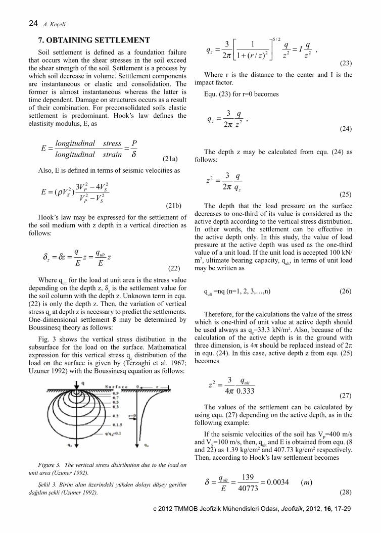
Fig. 3 shows the vertical stress distibution in the subsurface for the load on the surface. Mathematical expression

for this vertical stress qz distribution of the load on the surface is given by (Terzaghi et al. 1967; Uzuner 1992)

with the Boussinesq equation as follows:

Figure 3. The vertical stress distribution due to the load on unit area (Uzuner 1992).

#ekil 3. Birim alan üzerindeki yükden dolayı dü!ey gerilim da"ılım !ekli (Uzuner 1992).

22

2/5

2)/(1

1

2

3

z

qI

z

q

zrqz =!

"

#$%

&

+=

' , (23)

Where r is the distance to the center and I is the impact factor.

Equ. (23) for r=0 becomes

22

3

z

qqz

!= , (24)

(22)

Where qult

for the load at unit area is the stress value depending on the depth z, δ

z is the settlement value for

the soil column with the depth z. Unknown term in equ. (22) is only the depth z. Then, the variation of vertical stress q

z at depth z is necessary to predict the settlements.

One-dimensional settlement δ may be determined by Boussinesq theory as follows:

Fig. 3 shows the vertical stress distibution in the subsurface for the load on the surface. Mathematical expression for this vertical stress q

z distribution of the

load on the surface is given by (Terzaghi et al. 1967; Uzuner 1992) with the Boussinesq equation as follows:


Şekil 3. Birim alan üzerindeki yükden dolayı düşey gerilim dağılım şekli (Uzuner 1992).

16


follows:

zE

qz

E

qz ult

z === !! (22)










22

2/5

2)/(1

1

2

3

z

qI

z

q

zrqz =!

"

#$%

&

+=

' , (23)



22

3

z

qqz

!= , (24)

(23)



16


follows:

zE

qz

E

qz ult

z === !! (22)










22

2/5

2)/(1

1

2

3

z

qI

z

q

zrqz =!

"

#$%

&

+=

' , (23)



22

3

z

qqz

!= , (24)

(24)

The depth z may be calculated from equ. (24) as follows:

17


zq

qz

!2

32= (25)

The depth that the load pressure on the surface decreases to one-third of its value is considered as the active

depth according to the vertical stress distribution. In other words, the settlement can be effective in the active

depth only. In this study, the value of load pressure at the active depth was used as the one-third value of a unit

load. If the unit load is accepted 100 kN/m2, ultimate bearing capacity, qult, in terms of unit load may be written

as

qult =nq (n=1, 2, 3,…,n) (26)

Therefore, for the calculations the value of the stress which is one-third of unit value at active depth should be

used always as qz=33.3 kN/m2. Also, because of the calculation of the active depth is in the ground with three

dimension, is 4( should be replaced instead of 2( in equ. (24). In this case, active depth z from equ. (25)

becomes

333.04

32 ultqz!

= (27)

The values of the settlement can be calculated by using equ. (27) depending on the active depth, as in the

following example:

If the seismic velocities of the soil has VP=400 m/s and VS=100 m/s, then, qult and E is obtained from equ. (8 and

22) as 1.39 kg/cm2 and 407.73 kg/cm

2 respectively. Then, according to Hook’s law settlement becomes

)(0034.040773

139m

E

qult===! (28)

Where ' is the settlement for unit value. Under this condition, the active depth from equ. (25)

z = 10 m (29)

is obtained. The value of the total elastic settlement for the active depth z=10 m becomes

)(034.0100034.0 mxzE

qz ult

z ==== !! (30)

or 'z=3.4 cm (31)

(25)

The depth that the load pressure on the surface decreases to one-third of its value is considered as the active depth according to the vertical stress distribution. In other words, the settlement can be effective in the active depth only. In this study, the value of load pressure at the active depth was used as the one-third value of a unit load. If the unit load is accepted 100 kN/m2, ultimate bearing capacity, q

ult, in terms of unit load

may be written as

qult

=nq (n=1, 2, 3,…,n) (26)

Therefore, for the calculations the value of the stress which is one-third of unit value at active depth should be used always as q

z=33.3 kN/m2. Also, because of the

calculation of the active depth is in the ground with three dimension, is 4π should be replaced instead of 2π in equ. (24). In this case, active depth z from equ. (25) becomes

17


zq

qz

!2

32= (25)





as

qult =nq (n=1, 2, 3,…,n) (26)




becomes

333.04

32 ultqz!

= (27)


following example:


22) as 1.39 kg/cm2 and 407.73 kg/cm


)(0034.040773

139m

E

qult===! (28)


z = 10 m (29)


)(034.0100034.0 mxzE

qz ult

z ==== !! (30)

or 'z=3.4 cm (31)

(27)

The values of the settlement can be calculated by using equ. (27) depending on the active depth, as in the following example:

If the seismic velocities of the soil has VP=400 m/s

and VS=100 m/s, then, q

ult and E is obtained from equ. (8

and 22) as 1.39 kg/cm2 and 407.73 kg/cm2 respectively. Then, according to Hook’s law settlement becomes

17


zq

qz

!2

32= (25)





as

qult =nq (n=1, 2, 3,…,n) (26)




becomes

333.04

32 ultqz!

= (27)


following example:


22) as 1.39 kg/cm2 and 407.73 kg/cm


)(0034.040773

139m

E

qult===! (28)


z = 10 m (29)


)(034.0100034.0 mxzE

qz ult

z ==== !! (30)

or 'z=3.4 cm (31)

(28)



25

Where δ is the settlement for unit value. Under this condition, the active depth from equ. (25)

z = 10 m (29)


17


zq

qz

!2

32= (25)





as

qult =nq (n=1, 2, 3,…,n) (26)




becomes

333.04

32 ultqz!

= (27)


following example:


22) as 1.39 kg/cm2 and 407.73 kg/cm


)(0034.040773

139m

E

qult===! (28)


z = 10 m (29)


)(034.0100034.0 mxzE

qz ult

z ==== !! (30)

or 'z=3.4 cm (31)

(30)

or

17


zq

qz

!2

32= (25)





as

qult =nq (n=1, 2, 3,…,n) (26)




becomes

333.04

32 ultqz!

= (27)


following example:


22) as 1.39 kg/cm2 and 407.73 kg/cm


)(0034.040773

139m

E

qult===! (28)


z = 10 m (29)


)(034.0100034.0 mxzE

qz ult

z ==== !! (30)

or 'z=3.4 cm (31) (31)

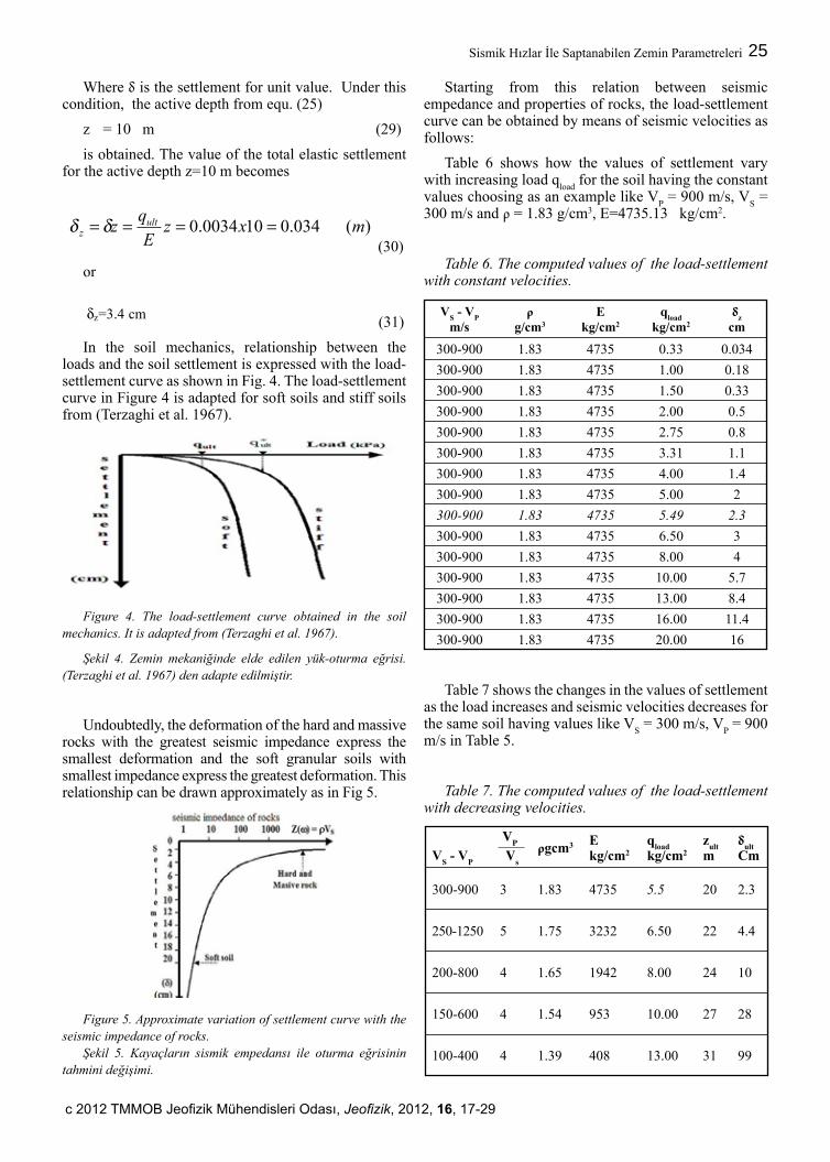
In the soil mechanics, relationship between the loads and the soil settlement is expressed with the load-settlement curve as shown in Fig. 4. The load-settlement curve in Figure 4 is adapted for soft soils and stiff soils from (Terzaghi et al. 1967).

Figure 4. The load-settlement curve obtained in the soil mechanics. It is adapted from (Terzaghi et al. 1967).

Şekil 4. Zemin mekaniğinde elde edilen yük-oturma eğrisi. (Terzaghi et al. 1967) den adapte edilmiştir.

Undoubtedly, the deformation of the hard and massive rocks with the greatest seismic impedance express the smallest deformation and the soft granular soils with smallest impedance express the greatest deformation. This relationship can be drawn approximately as in Fig 5.

Figure 5. Approximate variation of settlement curve with the seismic impedance of rocks.

Şekil 5. Kayaçların sismik empedansı ile oturma eğrisinin tahmini değişimi.

Starting from this relation between seismic empedance and properties of rocks, the load-settlement curve can be obtained by means of seismic velocities as follows:

Table 6 shows how the values of settlement vary with increasing load q

load for the soil having the constant

values choosing as an example like VP = 900 m/s, V

S =

300 m/s and ρ = 1.83 g/cm3, E=4735.13 kg/cm2.

Table 6. The computed values of the load-settlement with constant velocities.

VS - V

P

m/sρ

g/cm3

Ekg/cm2

qload

kg/cm2

δz

cm

300-900 1.83 4735 0.33 0.034

300-900 1.83 4735 1.00 0.18

300-900 1.83 4735 1.50 0.33

300-900 1.83 4735 2.00 0.5

300-900 1.83 4735 2.75 0.8

300-900 1.83 4735 3.31 1.1

300-900 1.83 4735 4.00 1.4

300-900 1.83 4735 5.00 2

300-900 1.83 4735 5.49 2.3

300-900 1.83 4735 6.50 3

300-900 1.83 4735 8.00 4

300-900 1.83 4735 10.00 5.7

300-900 1.83 4735 13.00 8.4

300-900 1.83 4735 16.00 11.4

300-900 1.83 4735 20.00 16

Table 7 shows the changes in the values of settlement as the load increases and seismic velocities decreases for the same soil having values like V

S = 300 m/s, V

P = 900

m/s in Table 5.

Table 7. The computed values of the load-settlement with decreasing velocities.

VS - V

P

ρgcm3 Ekg/cm2

qload

kg/cm2z

ultm

δult

Cm

300-900 3 1.83 4735 5.5 20 2.3

250-1250 5 1.75 3232 6.50 22 4.4

200-800 4 1.65 1942 8.00 24 10

150-600 4 1.54 953 10.00 27 28

100-400 4 1.39 408 13.00 31 99

VP

Vs

A. Keçeli


26

Fig.6 shows the change shape of the load-settlement curve ploted according to the values in Table 6 and in Table7.

Figure 6. The load-settlement curve obtained by means of seismic velocities.

Şekil 6. Sismik hızlar vasıtasıyla elde edilen yük oturma eğrisi.

Figure 6 shows that both shear failure and settlement starts as the load increases. It is seen that the load-settlement curve obtained by means of seismic velocities as in Fig. 6 and load-settlement curve in the soil mechanics in Fig. 5 have the similar variation.

Braja (1993) expressed that the value of the deformation generated in the seismic wave propagation is in the range like (10-2 – 10-4). According to these similar changes of the two load-settlement curves, it is understood that the value of small deformation generated in the seismic wave propagation is not important for the determination of the soil bearing capacity and settlement.

8. OBTAINING SUBGRADE REACTION COEFFICIENT

The coefficient of subgrade reaction, ks, is a concept

that is valid only at soil-foundation interface. The properties of the soil deformation are defined with the subgrade reaction. The subgrade reaction is also defined as a soil settlement under the certain stress. Foundation-ground interaction has been one of the challenging problems in geotechnical engineering. Various methods have been proposed for evaluating k

s. Many researches

have investigated the effective factors and determination approaches of k

s (Terzaghi, 1955; Bowles 1982). There

is no direct laboratory procedure for determining the value of the subgrade reaction coefficient. Because of the complexity of soil behavior, subgrade reaction in soil-foundation interaction problems is replaced by a more simple system called subgrade model. One of the

most common and simple models is an anolog of linear elastic springs. Evaluation of the numerical values of k

s is one of the most complex problems in geotechnical

engineering. Main problem with the accuracy of ks

relations is related to evaluation of the elasticity modulus, E. The elasticity modulus is the only factor by which the effect of subsurface soil properties on the value of k

s

can be examined. However, geophysical study has the advantage to obtain the elasticity modulus accurately and quickly by means of seismic velocities as follows:

Subgrade reaction coefficient, ks, is defined generally

in a similar way to the definition of Hook’s law as follows:

21

that the value of small deformation generated in the seismic wave propagation is not important for the

determination of the soil bearing capacity and settlement.


The coefficient of subgrade reaction, ks, is a concept that is valid only at soil-foundation interface. The properties

of the soil deformation are defined with the subgrade reaction. The subgrade reaction is also defined as a soil

settlement under the certain stress. Foundation-ground interaction has been one of the challenging problems in

geotechnical engineering. Various methods have been proposed for evaluating ks. Many researches have

investigated the effective factors and determination approaches of ks (Terzaghi, 1955; Bowles 1982). There is no

direct laboratory procedure for determining the value of the subgrade reaction coefficient. Because of the

complexity of soil behavior, subgrade reaction in soil-foundation interaction problems is replaced by a more

simple system called subgrade model. One of the most common and simple models is an anolog of linear elastic

springs. Evaluation of the numerical values of ks is one of the most complex problems in geotechnical

engineering. Main problem with the accuracy of ks relations is related to evaluation of the elasticity modulus, E.

The elasticity modulus is the only factor by which the effect of subsurface soil properties on the value of ks can

be examined. However, geophysical study has the advantage to obtain the elasticity modulus accurately and

quickly by means of seismic velocities as follows:

Subgrade reaction coefficient, ks, is defined generally in a similar way to the definition of Hook’s law as follows:

32

/)(

)/(mkN

m

mkNqqks

!!== (32)

ks may be written in terms of active depth z as follows:

z

ults

qk

!= (33)

If equ. (32) is replaced in equ. (33), then, a subgrade reaction coefficient may be defined depending on the active

depth z and elasticity modulus as

n

S

z

Ek = (34)

The value of the subgrade reaction coefficient can be calculated by using equ. (32 or 33) depending on the active

depth, as in the following example:

(32)

ks may be written in terms of active depth z as

follows:

21

that the value of small deformation generated in the seismic wave propagation is not important for the

determination of the soil bearing capacity and settlement.


The coefficient of subgrade reaction, ks, is a concept that is valid only at soil-foundation interface. The properties

of the soil deformation are defined with the subgrade reaction. The subgrade reaction is also defined as a soil

settlement under the certain stress. Foundation-ground interaction has been one of the challenging problems in

geotechnical engineering. Various methods have been proposed for evaluating ks. Many researches have

investigated the effective factors and determination approaches of ks (Terzaghi, 1955; Bowles 1982). There is no

direct laboratory procedure for determining the value of the subgrade reaction coefficient. Because of the

complexity of soil behavior, subgrade reaction in soil-foundation interaction problems is replaced by a more

simple system called subgrade model. One of the most common and simple models is an anolog of linear elastic

springs. Evaluation of the numerical values of ks is one of the most complex problems in geotechnical

engineering. Main problem with the accuracy of ks relations is related to evaluation of the elasticity modulus, E.

The elasticity modulus is the only factor by which the effect of subsurface soil properties on the value of ks can

be examined. However, geophysical study has the advantage to obtain the elasticity modulus accurately and

quickly by means of seismic velocities as follows:

Subgrade reaction coefficient, ks, is defined generally in a similar way to the definition of Hook’s law as follows:

32

/)(

)/(mkN

m

mkNqqks

!!== (32)

ks may be written in terms of active depth z as follows:

z

ults

qk

!= (33)

If equ. (32) is replaced in equ. (33), then, a subgrade reaction coefficient may be defined depending on the active

depth z and elasticity modulus as

n

S

z

Ek = (34)

The value of the subgrade reaction coefficient can be calculated by using equ. (32 or 33) depending on the active

depth, as in the following example:

(33)

If equ. (32) is replaced in equ. (33), then, a subgrade reaction coefficient may be defined depending on the active depth z and elasticity modulus as

nS z

Ek = (34)

The value of the subgrade reaction coefficient can be calculated by using equ. (32 or 33) depending on the active depth, as in the following example:

The value of the subgrade reaction coefficient for the active depth z=10 m from equ.(33) becomes

22

The value of the subgrade reaction coefficient for the active depth z=10 m from equ.(33) becomes

3/4088

034.0

139mkN

qk

z

ultS ===

! (35)

(Bowles 1998) gave the following emprical formulae for estimating the coefficient of subgrade reaction using an

ultimate bearing capacity for only granular soils:

kBowles = 40 x qult kN/m3

(36)

When qult= 139 (kN/m2)

is replaced in equ. (36), kBowles is obtained as

kBowles = 40 x 139= 5560 kN/m3

(37)

the emprical values of the subgrade reaction coefficient Bowles gave are in the range of (4800-128000) kN/m3

or ton/m3. Table 8 shows the comparison of the values of the subgrade reaction coefficients calculated from the

relations in this study and Bowles emprical relation for seismic velocities of several soil and rocks. According to

table 8, it is seen that settlement increases and subgrade reaction reduces with decreasing shear wave velocity.

Also, it is seen that the values of ks and kBowles close to each other in an appropriate limit according to Bowles

experimental values. Such that, while kBowles =5560 (kN/m3), ks= 4088 (kN/m

3) for loose sand soils with (VS -

VP)= (100-400) m/s and while kBowles = 41600 (kN/m3), k= 53489 (kN/m

3) for stiff sand soils with (VS - VP)=

(500-1250) m/s.

(35)

(Bowles 1998) gave the following emprical formulae for estimating the coefficient of subgrade reaction using an ultimate bearing capacity for only granular soils:

kBowles

= 40 x qult

kN/m3 (36)

When qult

= 139 (kN/m2) is replaced in equ. (36), k

Bowles is obtained as

kBowles

= 40 x 139= 5560 kN/m3 (37)

the emprical values of the subgrade reaction coefficient Bowles gave are in the range of (4800-



27

128000) kN/m3 or ton/m3. Table 8 shows the comparison of the values of the subgrade reaction coefficients calculated from the relations in this study and Bowles emprical relation for seismic velocities of several soil and rocks. According to table 8, it is seen that settlement increases and subgrade reaction reduces with decreasing

shear wave velocity. Also, it is seen that the values of k

s and k

Bowles close to each other in an appropriate limit

according to Bowles experimental values. Such that, while k

Bowles =5560 (kN/m3), k

s= 4088 (kN/m3) for loose

sand soils with (VS - V

P)= (100-400) m/s and while k

Bowles

= 41600 (kN/m3), k= 53489 (kN/m3) for stiff sand soils with (V

S - V

P)=(500-1250) m/s.

Table 8. shows the comparison of the theoretical and Bowles experimental relations.

VS - V

P

ρg/cm3 qult.

kg/cm2q

akg/cm2

Ekg/cm2

zult.

mδ

ult.cm

ks

kN/m3k

Bow =40q

ult.kN/m3

4000-6000 1.5 3.5 140 93 1232000 100 1.1 1232000 560000

2000-3000 1.5 2.94 59 39 258940 65 1.5 398548 235400

1000-2000 2 2.47 25 12 65973 42 1.6 156613 98960

1000-1500 1.5 2.47 25 16 54428 42 1.9 129225 98960

700-1400 2 2.26 16 7.9 29494 34 1.8 87508 63360

500-1250 2.5 2.1 10 4.2 14609 27 1.9 53489 41600

300-900 3 1.83 55 1.8 4735 20 2.3 23869 21960

250-1250 5 1.75 44 0.87 3232 18 2.4 18268 17480

200-800 4 1.65 3.3 0.83 1942 15 2.6 12614 13240

150-600 4 1.54 2.3 0.58 953 13 3.2 7219 9240

100-400 4 1.39 1.4 0.35 408 10 3.4 4097 5560

50-250 5 1.2 0.6 0.12 89 6.6 4.4 1353 2400

9. CONCLUSION

The results obtained in this investigation can be summarized as follows:

1- The ultimate bearing capacities of the soils and rocks can be expressed with seismic shear wave impedances of the soils and rocks.

2- The similarity between the coefficients of the safety factor depending also on the soil properties and the values of the V

p /V

s velocity ratio shows that the V

p /

Vs velocity ratio can be used as a safety factor.

3- The relation of the allowable bearing capacity obtained from the seismic velocities includes shear modulus.

4- When the Vp /V

s velocity ratio as a safety factor is

used for the soil saturated with water, there is no need to use any reduction operation to decrease ultimate bearing capacity.

5- It was seen that the densities expressed depending on the shear wave velocity is more appropriate.

6- The allowable bearing capacity including spread footing of foundatio shape can be obtained.

7-Utilizing the Boussinesq equation, subgrade reaction and settlement can be determined by using the ultimate bearing capacity and elasticity modulus obtained from the seismic velocities.

8- The load-settlement curve obtained by means of seismic velocities and the load-settlement curve in the soil mechanics show the similar variation.

9- The results obtained from seismic velocities are more stable, consistent and reliable when compared with those of the conventional method.

10- The application of the technique developed in this study does not depend on personal preferences.

As a consequence, it is possible to obtain the reliable additional knowledge about the safety bearing capacity, subgrade reaction and settlement values while the structural geology is determined. Furthermore, the developed technique here is quick and cost effective. If the parameters of soil mechanics and the proposed seismic technique are used together, very useful information may be obtained to interpret the properties of the underground.

VP

Vs

A. Keçeli


28

10. APPENDIX

Due to the use of c. g. s. unit for calculations of bearing capacity in Turkey, it will be useful to show transformation of m. k. s. and c. g. s. unit. Newton is defined as N (kg.m/s2). Where m/s2 is accelaration of the earth, (g) and as well known, the approximately value of g is 10 m/s2 or 1000 cm/s2.

25

222

2

224

6

2

3

24

24

2

2

2

2

2

100

110

10

1010

10

.

10

10

cm

kgkPa

s

cm

cm

kg

s

cm

cm

kg

s

cm

cm

kgkkPa

cm

s

cmkg

m

s

mkg

m

NPa

==

==

===

As an example; qa in transformation of m.k.s. and c.g.s. units for VP = 900 m/s, VS = 300 m/s and " = 1.83

g/cm3 becomes

In m.k.s. unit:

kPaV

V

F

Vq

p

s

S

Sa 183

900

)1.0()300(3.18)1.0()1.0( 22

====!!

kPam

kN

cm

kg

mkNs

cm

cm

g

s

cm

cm

g

s

m

m

kkgs

s

m

s

m

m

kkgs

s

m

s

m

m

TsgVq Sult

100

1

100

1

/100

10

10

1.0101.0101.0

22

2

22224

6

222323

==

==

==== !

In c.g.s. unit:

)/(83.1)183(100

1

100

1 22

cmkgkPaV

Vq

p

sa ==!

"

As an example; qa in transformation of m.k.s. and

c.g.s. units for VP = 900 m/s, V

S = 300 m/s and ρ = 1.83

g/cm3 becomes

In m.k.s. unit:

25

222

2

224

6

2

3

24

24

2

2

2

2

2

100

110

10

1010

10

.

10

10

cm

kgkPa

s

cm

cm

kg

s

cm

cm

kg

s

cm

cm

kgkkPa

cm

s

cmkg

m

s

mkg

m

NPa

==

==

===


g/cm3 becomes

In m.k.s. unit:

kPaV

V

F

Vq

p

s

S

Sa 183

900

)1.0()300(3.18)1.0()1.0( 22

====!!

kPam

kN

cm

kg

mkNs

cm

cm

g

s

cm

cm

g

s

m

m

kkgs

s

m

s

m

m

kkgs

s

m

s

m

m

TsgVq Sult

100

1

100

1

/100

10

10

1.0101.0101.0

22

2

22224

6

222323

==

==

==== !

In c.g.s. unit:

)/(83.1)183(100

1

100

1 22

cmkgkPaV

Vq

p

sa ==!

"

In c.g.s. unit:

25

222

2

224

6

2

3

24

24

2

2

2

2

2

100

110

10

1010

10

.

10

10

cm

kgkPa

s

cm

cm

kg

s

cm

cm

kg

s

cm

cm

kgkkPa

cm

s

cmkg

m

s

mkg

m

NPa

==

==

===


g/cm3 becomes

In m.k.s. unit:

kPaV

V

F

Vq

p

s

S

Sa 183

900

)1.0()300(3.18)1.0()1.0( 22

====!!

kPam

kN

cm

kg

mkNs

cm

cm

g

s

cm

cm

g

s

m

m

kkgs

s

m

s

m

m

kkgs

s

m

s

m

m

TsgVq Sult

100

1

100

1

/100

10

10

1.0101.0101.0

22

2

22224

6

222323

==

==

==== !

In c.g.s. unit:

)/(83.1)183(100

1

100

1 22

cmkgkPaV

Vq

p

sa ==!

"

REFERENCES Bowles, J. E. 1998, Foundation Analysis and Design, 6th ed.,

McGrow-Hill International press.

Braja, M. D. 1993, Principles of soil dynamics: PWS-Kent Publishing Company.

Brown, D.W. 1992, Engineering and Design Bearing Capacity of Soils, (Engineer Manual) Department of the Army, U.S. Army Corps of Engineers, Washington, DC 20314-1000

Carvalho, J., Dias, R., Pinto, C., Leote, J. and Mendes, V. L. 2009, SPT seismic hazard seismic refraction soil classification. and Geotechnical Data Applied to the Soil Microzoning of Western Algarve, Portugal. European Journal of Environmental and Enginnering Geophysics 5, 3-14.

Fu D., Sullivan, E.C. and Marfurt, K. 2006, Rock-Property and Seismic-Attribute Analysis of a chert reservoir in Devenian Thirty-one Formation: Geophysics, Vol. 71, No.5.

Gardner, G. H. F., Gardner, L. W. and Gregory, A. R. 1974. Formation velocity and density—the diagnostic basics for stratigraphic traps, Geophysics 39, 770-–780.

Guliev, E. 2007, Vp/Vs estimation from Multicomponent Seismic Data for Improved Characterization of a Tight sanstone Gas reservoir, Colorado School of Mines , A thesis for the degree of Master of Science (Geophysics) Colorado School of Mine.

Hamada, G. M. 2004, Reservoir Fluids Identification Using Vp/Vs Ratio? Oil & Gas Science and Technology-Rev. IFP, Vol.59,No.6, pp.n649-654.

Hardin, B.O. and Black W.L. 1968, Vibration Modulus of Normally Consalidated Clays, Journal of the Soil Mechanics and Foundation Division, ASCE, Vol.94, No.SM2, pp. 353-369.

Hardin, B.O. and Drnevich V.P. 1972. Shear Modulus and Damping in Soils. J. Soil Mech. and Found. Div.,ASCE, 98 SM7: 667-692.

Hicks, G.J. 2006, Extended Elastic İmpedance and Its Relation to AVO Crossplotting and Vp/Vs EAGE 68th Conference, Vienna, Austria.

Imai, T. and Yoshimura M. 1972. The relation of Mechanical Properties of Soils to P and S Wave Velocities for Soil Ground in Japan. Urana Research Institute,OYO Corp.

Imai, S. (1975), An investigation to geophysical prospecting for civil purposes OYO Co-operation, Tokyo, Japan.

Imai, T. and Yoshimura M. 1976, The relation of Mechanical Properties of Soils to P and S Wave Velocities for Soil Ground in Japan. Urana Research Institute, OYO Corp.

Jongmans, D. 1992, The application of Seismic Methods for Dynamic Characterization of Soils. Bulletin of International Association of Engineering Geology. 46: 63-69.

Kaptan, K., Ozdemir Z. and Tezcan S. 2011, Review A refined formula for the allowable soil pressure using shear wave velocities: The Journal of Soil Science and Environmental Management, Vol. 2,7, pp. 175-183.

Keçeli, A. D. 1990, The determination of the Bearing Capacity by means of the seismic method: Jeofizik 4, 83-92. ( in Turkish).

Keçeli, A. D. 2000, The Determination of the Presumptive Bearing Capacity by means of the Seismic Method: JEOFİZİK, Cilt: 14, Sayı: 1-2.( in Turkish).

Keçeli, A. D. 2009. Uygulamalı Jeofizik, TMMOB Jeofizik Müh. Odası Eğitim yayınları No:9, s.479.

Lankston, R. W. 1990, High-Resolution Refraction Seismic Data Acquisition and Interpretation: in Geotechnical and environmental Geophysics. Soc. Expl. Geophys. Vol., I, 45-73.



29

Meyerhof, G.G. 1974, Ultimate bearing capacity of footing on sand layer overlying clay. Canadian Geotechnical Journal, 11, pp. 223-229.

Moreno, C. Huffman A., and Bertagne A. (2003), The Vp/Vs Inversion Procedure: A Methodology for Shallow Water Flow (SWF) Prediction from Seismic Analysis of Multicomponent Data. Offshore Technology Conference, Houston, Texas.

Ohkubo, T. and Terasaki A. 1976, Physical property and seismic wave velocity of rocks, OYO Corporation, Japan.

Othman, A. A. 2005, Construed geotechnical characteristics of foundation beds by seismic measurements. J. Geophys. Eng. 2 126–138.

Parry, R. H.G. 1977, Estimating bearing capacity of sand from SPT values JGED ASCE 103:Gt.9 pp1014-1043.

Phillips, D. E., Han, D. H. and Zoback M. D. 1989, Emprical Relationships among Seismic Velocity, Effect Pressure, Porosity, and Clay Content in Sandstone. Geophysics,54:(1) 82-89.

Pişen, S. ve Pekşen E. 2009, Sığ Zeminler için Farklı Yöntemlerden Elde Edilen Zemin Emniyet Gerilmesi Değerlerinin Karşılaştırılması: Uygulamalı Yerbilimleri Sayı:2, 36-46.

Prakla, 1986, Seismos A. G. Buchhholzer Str. 100 P. O. B 510530 D-300 Hannover 51.

Seed, H.B., Wong, R.T., Idriss, E.M., and Tokimatsu, K. 1984, Moduli and Damping Factors for Dynamic Analyses of Cohesionless Soils, Report No. UCB/EERC - 84/11, Earthquake Engineering Research Center, University of California, Berkeley.

Sternberg, B. K., Poulton, M. M. and Thomas S. J. 1990, Geophysical investigations in Support of the Arizona SSC project.( In Geotechnical and Enviromental Geophysics, S.E.G. V.III:211-228).

Stuempel, H, Kahler S., Meissner R. and Milkereit B. 1984, The use of Seismic Shear Waves and Compressional Waves for Lithological Problems of Shallow Sediments: Geophys. Prospect. 32 662–75.

Tatham, R.H. 1982, Vp/Vs and Lithology. Geophysics, 47: 336-344.

Terzaghi, K. 1955, Evaluation of Coefficient of Subgrade Reaction, Geotechnique, Vol. 5, No. 4,297-326.

Terzaghi, K. and Peck R.B. 1967, Soil Mechanics in Engineering Practice. 2nd ed., John Wiley & Sons, London.

Tezcan, S.S., Ozdemir, Z. and Keceli, A. 2009, Seismic Technique to Determine the Allowable Bearing Pressure for Shallow Foundandations in Soils and Rocks, Acta Geophysica, Vol.57, No. 2, pp.400-412.

Tezcan, S. and Ozdemir Z. 2011, A Refined Formula for the Allowable Soil Pressure Using Shear Wave Velocities: The Open Civil Engineering Journal, 5, 1-8 1

Uyanık, O. 2010. Compressional and Shear-Wave Velocity Measurements in Unconsolidated the Top-Soil and Comparison of the Results. International Journal of the Physical Sciences Vol. 5(7), pp. 1034-1039.

Uyanık, O. 2011. The Porosity of Saturated Shallow Sediments from Seismic Compressional and Shear Wave Velocities, Journal of Applied Geophysics,73(1), 16-24.

Uzuner, B.A. 1992, Fundamental Soil Mechanics, Chamber of Civil Engineering, Trabzon/Turkey (in Turkish).

Venkatramaiah, C. 1993, Geotechnical Engineering, John Wiley & Sons.

Vesic, A. B. 1961 Beams on Elastic Subgrade and Winkler’s Hypothesis, Proc. 5th

Wang, Z. 2001, Fundamentals of Seismic Rock Physics: Geophysics, Vol. 66, No. 2; P. 398–412.

Int. Conf. on Soil Mechanic and Foundation Engineering, Paris: 845-850.

Willkens, R., Simmons G. and Caruso L. 1984, The ratio Vp/

Vs as a Discriminant of Composition for Siliceous Limestones.

Geophysics, 49 ( 11) 1850-1860.

Wyllie, D. C. 1992, Foundations on Rock. E & FN Spon, London.

soil parameters which can be determined with seismic

Documents