software user's manual for the coupled ocean/atmosphere
TRANSCRIPT

Naval Research LaboratoryMonterey, CA 93943-5502
NRLIMR/7543--96-7227
Software User's Manual for the CoupledOcean/Atmosphere Mesoscale PredictionSystem (COAMPS)TRACY HAACK
Atmospheric Dynamics & Prediction BranchMarine Meteorology Division
November 1996
Approved for public release; distribution unlimited.
------

-V

REPORT DOCUMENTATION PAGE [Approv____ ed_ _&AX~~~~~~~~~~~~~~~~~~~~~ OMB No.~e_ 0740188;> inas ;A~ niuir [<+min ~rhn i~n ~
Public reporting burden for this collection of intornation is estimated to average 1 nour per response, Imclu9 mIea Ine *.. --i-wmg msr ....o.s, ssa..... 1-n- -xs.. g sources, gathering and maintaining the data needed, and completing and reviewing the collection of information. Send comments regarding this burden or any other aspect of thiscollection of Information. including suggestions for reducing this burden, to Washington Headquarters Services, Directorate for Information Operations and Reports, 1215hfferson Davis Highway, Suite 1204, Arlington, VA 222024302, and to the Office of Management and Budget, Paperwork Reduction Project (0704-0188), Washington, DC 20503.
Agency Use Only (Leave Blank). 2. Report Date. 3. Report Type and Dates Covered.
1W I November 1996 Final
4. Title and Subtitle. 5. Funding Numbers.
Software User's Manual for the Coupled Ocean/Atmosphere Mesoscale Prediction PE 0 & MNSystem (COAMPS) PN NA
AN DN 153-174
6. Author(s).Tracy Haack
7. Performing Organization Name(s) and Address(es). 8. Performing Organization
Naval Research Laboratory Reporting Number.Marine Meteorology Division NRL/MR/7534- - 96- - 7227Monterey, CA 93943-5502
8. Sponsoring/Monitoring Agency Name(s) and Address(es).10. Sponsoring/Monitoring Agency
Naval Meteorology & Oceanography Report Number.Command (CNMOC)
11. Supplementary Notes.
a. Distribution /Availability Statement 12b. Distribution Code.
Approved for public release; distribution unlimited-
13. Abstract (Maximum 200 words).
The Navy has developed a nonhydrostatic fully coupled ocean/atmosphere model, The CoupledOcean/Atmosphere Mesoscale Prediction System (COAMPS), for predicting and simulatingmeteorological processes on meso to micro scales of motion. This document covers only theatmospheric portion and is based upon version 2.0 of the COAMPS code. The atmospheric modelmay be initialized with idealized fields or real data adjusted by observations. Detaileddescriptions and diagrams of the COAMPS directory structure and coding framework is given tofamiliarize the user with the system. In addition, COAMPS numerous input parameters aredefined and categorized to aid the user in manipulating the code to suit a variety of possible casestudies. Finally, the user is taken through a step-by-step procedure for implementing and workingwith the system and for setting up and submitting a COAMPS model run.
14. Subject Terms. 15. Number of Pages.
Coupled Ocean/Atmosphere Mesoscale Prediction System (COAMPS) 8816. Price Code.
Security Classification 18. Security Classification 19. Security Classification 20. Limitation of abstract.of Report. of This Page. of Abstract.
UNCLASSIFIED UNCLASSIFIED UNCLASSIFIED Same as report
NSN 7540-01-280-5500 Standard Form 298 (Rev. 2-89)Prescribed by ANSI Std. Z39-18298-102
IA
4
-AM
i

0
6
0
4
0

Tal fCntnsPg1. Scope 1
2. Reference Documents 22.1. COAMPS Model Descriptions 22.2. COAMPS Simulations 22.3. Dynamics 32.4. Physics 32.5. Numerics 42.6. COAMPS Graphics 52.7. Analysis 5
3. System Overview 63.1. COAMPS General Features 6
3.1.1. Driver Programs and Namelists 63.1.2. Model Domain Structure 83.1.3. Initial Conditions and COAMPS Databases 123.1.4. First Guess Fields and Data Assimilation 14
3.2. COAMPS Directory Structures 163.3. COAMPS Code 19
3.3.1. Analysis 193.3.1.1. Idealized Data 233.3.1.2. Real Data 23
3.3.2. Forecast 253.3.2.1. Reading Initial Conditions 273.3.2.2. Model Integration:
Forecast Loop and Atmospheric Model 303.3.2.3. Writing Output 35
4. Execution Procedure 394.1. Preparation Steps 394.2. COAMPS Input File: Gridnl, Coamnl and Mvoinl Namelists 41
4.2.1. Model Setup 414.2.1.1. Grid 414.2.1.2. Integration 424.2.1.3. Boundary Conditions 42
4.2.2. Case Study Setup 434.2.2.1. Analysis Fields 434.2.2.2. Model Physics 444.2.2.3. Numerical Damping 444.2.2.4. Additional Model Features 44
4.2.3. Data Manipulation 444.3. Submitting a COAMPS Job 45
iii
PageTable of Contents
List of Appendices Page
Appendix A: Sample makefile A-1Appendix B: Sample COAMPS user input file nfist.input B-1Appendix C: Input parameters: gridnlnamelist C-1Appendix D: Input parameters: coamni namelist D-1Appendix E: Three sample map projections, input parameters
and model domains E-1
iv

List of Figures
Figure 1:Figure 2:Figure 3a:Figure 3b:Figure 4:
Figure 5:Figure 6:Figure 7:Figure 8:Figure 9:Figure 10:Figure 1 1:
Figure E-1:Figure E-2:
Figure E-3:
Figure E-4:
Figure E-5:
Figure E-6:
Flow chart of the COAMPS driver programs.Schematic representation of three horizontally nested domains.Schematic representation of the vertical grid staggering.Schematic representation of the horizontal grid staggering.Schematic representation of the COAMPS data assimilationupdate cycleCOAMPS directory structure.Flow chart of input/output for the analysis routine.Flow chart of the analysis routine.Flow chart of input/output for the forecast routine.Flow chart of the forecast routine.Flow chart of the atmospheric model subroutine.Flow chart of the subroutines called by coamm.f that write outmodel data.Schematic representation of a mercator map projection.Example of a COAMPS horizontal domain using a mercatormap projection.Schematic representation of a lambert conformal mapprojection.Example of a COAMPS horizontal domain using a lambertconformal map projection.Schematic representation of a polar stereographic mapprojection.Example of a COAMPS horizontal domain using a polarstereographic map projection.
V
Page
791011-
15172022262830
36E-1
E-2
E-3
E-4
E-5
E-6

List of Tables
Table la:Table lb:Table 1c:Table 2:Table 3:Table 4:Table 5:Table 6:Table D-1:
Table E-1:
Table E-2:
Table E-3:
COAMPS 2D surface arrays.COAMPS 3D basic state arrays.COAMPS 3D prognostic arrays.COAMPS array naming convention.Standard machine settings for COAMPS compilation.COAMPS output file naming convention.Sigma level data and surface fields written out by COAMPS.Options for the 2nd run script input argument.Namelist input options for the TKE mixing length parameteriamxgl.Namelist input parameters and values for the mercatormap projection shown in Figure E-2.Namelist input parameters and values for the lambertconformal map projection shown in Figure E-4.Namelist input parameters and values for the polarstereographic map projection shown in Figure E-6.
Vi
Page
1213131418373845
D-1
E-1
E-3
E-5

Acknowledgments
Many helpful suggestions were given by reviewers Dr. Richard Hodur, Dr. WilliamThompson, Ms. Liana Zambresky, Dr. Teddy Holt and Ms. Patricia Phoebus of NRLMonterey. The assistance of Ms. Sue Chen in reorganizing the document is alsogratefully acknowledged. This work was sponsored by the Oceanographer of the Navy,and the Program Office at Space and Naval Warfare Systems Command (PMW-1 85),under program element 0603207N.
Vii

S

1. Scope
Numerical models have been an effective tool in the prediction of manygeophysical systems. Processes within the earth's two primary physical systems, theocean and atmosphere, directly impact Naval operations on the mesoscale and thelocal PBL scale. Consequently, accurate and efficient prediction on these scales is anecessity. Scientists now consider the ocean and atmosphere as separate but fullycoupled, two-way interactive fluids. Predicting the behavior of either fluid depends uponthe spatial and temporal forcing applied by the other. Thus, a single numericalprediction system combining an oceanic and an atmospheric model provides morerealistic representation of these two geophysical systems. Additionally in the pastdecade, increased computer power and technological advancements have improvedcomputational efficiency allowing larger models, with higher resolution, multi-nestedgrids and complicated physics, to be developed and run for real-time forecastingpurposes. When used in a research mode, the models also provide valuable insighttoward understanding complex mesoscale interactions. To fully utilize moderncomputer resources and to meet the growing need for high resolution, coupledoceanic/atmospheric forecasts, a new model has been developed by the NavalResearch Laboratory: The Coupled Ocean/Atmosphere Mesoscale Prediction System(COAMPS).
At present, COAMPS consists of two FORTRAN programs: an analysis programthat blends observations with first guess fields to provide initial conditions, and aforecast program containing a nonhydrostatic, quasi-compressible atmospheric modelwith complete physics schemes for predicting meso and micro scales of motion (i.e.time scales ranging from days to minutes and spatial scales ranging from thousands ofkilometers to a few meters). This system can be run using idealized or real data initialconditions with up to seven horizontally nested domains. Because the ocean forecastmodel of COAMPS currently is under development, it will be implemented at a laterdate. For this reason, this report documents only the atmospheric model. Moreover,the focus here is to provide a brief introduction to COAMPS, along with a quickreference guide for setting up and performing a COAMPS model run. It is not intendedas a complete description of the model physics or dynamics. Additional readingmaterial on COAMPS and related references are given in Section 2. An overview of theCOAMPS directory structures and the code is given in Section 3. In Section 4. theprocedure for executing a model run is described for either idealized or real dataassimilation process studies. This section is beneficial in assisting the new user andalso as a reference guide for identifying, defining and modifying relevant modelparameters. Appendices A-E provide sample files and tables that list and defineCOAMPS input parameters.
2. Reference Documents
2.1. COAMPS Model Descriptions
Haack, T.H., 1993: User's guide for the coupled ocean/atmosphere mesoscaleprediction system (COAMPS). NRL Memorandum Report 7214, November, 1993.
Hodur, R.M., 1993: Development and testing of the coupled ocean/atmospheremesoscale prediction system (COAMPS). NRL Memorandum Report 7213,November, 1993.
Hodur, R.M.: The U.S. Navy's coupled ocean/atmosphere mesoscale prediction system(COAMPS). Submitted to Mon. Wea. Rev.
Hodur, R.M. and J. Doyle, 1995: The coupled ocean/atmosphere mesoscale predictionsystem (COAMPS). Chapter in "Coastal Ocean Prediction", CRC Press, Boca Raton,Florida, 96 pp.
Xu, L., 1995: Incorporation of orography into the coupled ocean/atmosphere mesoscaleprediction system (COAMPS): formulation and validation tests. Chapter 3 in"The study of mesoscale land-air-sea interaction processes using anonhydrostatic model", Ph.D. dissertation, North Carolina State University, 336pp.
2.2. COAMPS Simulations
Doyle, J., 1995: Coupled ocean wave/atmosphere mesoscale model simulations ofcyclogenesis. Tellus, 47A,5:1, 766-778.
Hirschberg, P.A. and J. Doyle, 1995: An examination of pressure tendency mechanismsin an idealized simulation of extratropical cyclogenesis. Tellus, 47A5:1, 747-758.
Hodur, R.M.: Development and testing of the coupled ocean/atmosphere mesoscaleprediction system (COAMPS). NRL Memorandum Report 7533, November, 1993.
Thompson, W.T., T. Haack and J.D. Doyle, 1996: An investigation of the southerly surge.1996 NRL Review, 151-153.
Thompson, W.T., T. Haack, J.D. Doyle and S.D. Burk, 1996: A nonhydrostatic mesoscalesimulation of the 10-11 June 1994 trapped coastal wind reversal. Submitted to Mon.Wea. Rev.
2

Xu, L., S. Raman, R.V. Madala and R. Hodur, 1996: A non-hydrostatic modeling studyof surface moisture effects on mesoscale convection induced by sea breezecirculation. Meteorol. Atmos. Phys., 58,103-122.
2.3. Dynamics
Klemp, J.B. and R.B. Wilhelmson, 1978: The simulation of three-dimensional convectivestorm dynamics. J. Atmos. Sci., 35,1070-1096.
2.4. Physics
Businger, J.A., J.C. Wyngaard, Y. Izumi, and E.F. Bradley, 1971: Flux-profile relationshipsin the atmospheric-surface layer. J. Atmos. Sci., 28,181-189.
Deardorff, J.W., 1972: Numerical investigation of neutral and unstable planetaryboundary layers. J. Atmos. Sci., 29, 91-115.
Deardorff, J.W., 1978: Efficient prediction of ground surface temperature and moisturewith inclusion of a layer of vegetation. J. Geophys. Res., 83, 1889-1903.
Deardorff, J.W., 1980: Stratocumulus-capped mixed layers derived from a three-dimensional model. Bound. Layer Meteor., 18, 495-527.
Hogan, T.F. and T.E. Rosmond, 1991: The description of navy operational globalatmospheric prediction system's spectral forecast model. Mon. Wea. Rev., 119,1786-1815.
Harshvardhan, R.D., D. Randall and T. Corsetti, 1978: A fast radiation parameterizationfor atmospheric circulation models. J. Geophys. Res., 92, 1009-1016.
Louis, J.F., 1979: A parametric model of vertical eddy fluxes in the atmosphere. Bound.Layer Meteor., 17, 187-202.
Louis, J.F., M. Tiedtke and J.F. Geleyn, 1982: A short history of the operational PBL-parameterization at ECMWF, Workshop on Planetary Boundary Parameterization,ECMWF, Reading, 59-79.
Mellor, G.L. and T. Yamada, 1974: A hierarchy of turbulence closure models for planetaryboundary layers. J. Atmos. Sci., 31, 1791-1806.
Mellor, G.L. and T. Yamada, 1982: Development of a turbulence closure for geophysicalfluid problems. Rev. Geophys and Space Phys., 20, 851-875.
3

Rutledge S.A. and P.V. Hobbs, 1983: The mesoscale and microscale structure oforganization of clouds and precipitation in midlatitude cyclones. VIII: A model for the"seeder-feeder" in warmn-frontal rainbands. J. Atmos. Sci., 40,1185-1206.
Smagorinsky, J., 1963: General circulation experiments with the primitive equations: 1.The basic experiment. Mon. Wea. Rev., 91, 99-164.
Therry, G. and T. LaCarrere, 1983: Improving the eddy kinetic energy model for planetaryboundary layer description. Bound. Layer Meteor., 25, 63-88.
2.5. Numerics
Arakawa, A. and V.R. Lamb, 1974: Computational design of the UCLA general circulationmodel. Methods in Computational Physics, Vol. 17, Academic Press, 173-265.
Chorin, A.J., 1967: A numerical method for solving incompressible viscous flow problems.J. Comput. Phys., 2,12-16.
Cressman, G., 1959: An operational objective analysis system. Mon. Wea. Rev., 87,1367-374.
Dudhia, J., 1993: A nonhydrostatic version of the Penn State-NCAR mesoscale model:validation tests and simulation of an Atlantic cyclone and cold front. Mon. Wea. Rev.,121,1493-1513.
Durran D.R. and J.B. Klemp, 1983: A compressible model for the simulation of moistmountain waves. Mon. Wea. Rev., 111, 2341-2361.
Droegemeier, K.K. and R.B. Wilhelmson, 1987: Numerical simulation of thunderstormoutflow dynamics. Part I: Outflow sensitivity experiments and turbulence dynamics. J.Atmos. Sci., 44, 1180-1210.
Haltiner, G.J. and R.T. Williams, 1980: Numerical prediction and dynamic meteorology.John Wiley & Sons, Inc. 477 pp.
Hodur, R.M., 1987: Evaluation of a regional model with an update cycle. Mon. Wea. Rev.,115, 2707-2718.
Ikawa, M., 1988: Comparison of some schemes for nonhydrostatic models withorography. J. Meteor. Soc. Japan, 66, 753-776.
Klemp, J.B. and D.K. Lilly, 1978: Numerical simulation of hydrostatic mountain waves. J.Atmos. Sci., 35, 78-107.
4

Klemp, J.B. and R.B. Wilhelmson, 1978: The simulation of three-dimensional convectivestorm dynamics. J. Atmos. Sci., 35,1070-1096.
Miller, M.J. and A.J. Thorpe, 1981: Radiation conditions for the lateral boundaries oflimited area numerical models. Quart. J. R. Met. Soc., 107, 615-628.
Orlanski, I., 1976: A simple boundary condition for unbounded hyperbolic flows. J.Comput. Phys., 21, 251-269.
Robert, A.J., 1966: The investigation of a low order spectral form of the primitivemeteorological equations. J. Meteor. Soc. Japan, 44, 237-245.
Shamarock, W.C. and J.B. Klemp, 1992: The stability of time-split numerical methods forthe hydrostatic and the nonhydrostatic elastic equations. Mon. Wea. Rev., 120, 2109-2127.
2.6. COAMPS Graphics
Haack, T.H., 1992: Graphical display procedure for grid point model data. NRLTechnical Note 263, June, 1992.
Lewit, H. (CSC), 1993: Description and use of the ocards process management system.FNOC Model Dept. Tech. Note 4-93, September, 1993.
2.7. Analysis
Baker, N.L, 1992: Quality control for the navy operational atmospheric database. Wea.Forecasting, 7, 250-261.
Barker, E.H, 1992: Design of the navy's multivariate optimum interpolation analysissystem. Wea. Forecasting, 7, 527-528.
Goerss, J.S. and P.A. Phoebus, 1992: The Navy's operational atmospheric analysis.Wea. Forecasting, 7, 232-249.
5
3. System Overview
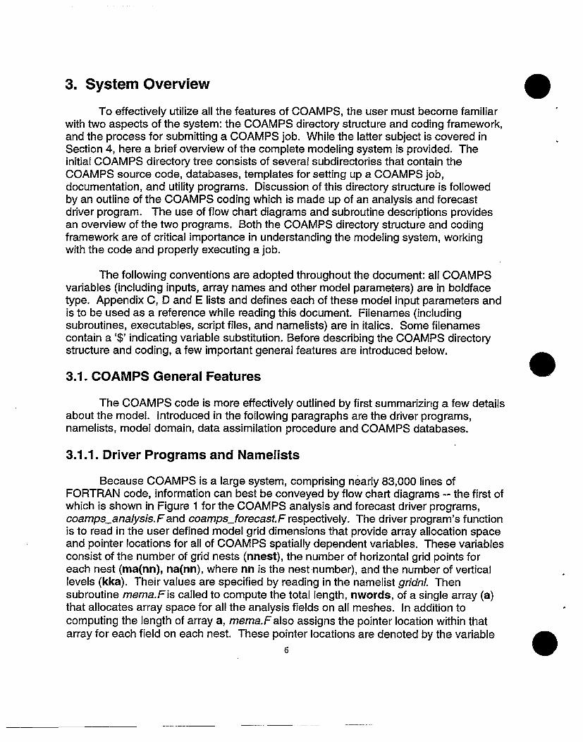
To effectively utilize all the features of COAMPS, the user must become familiarwith two aspects of the system: the COAMPS directory structure and coding framework,and the process for submitting a COAMPS job. While the latter subject is covered inSection 4, here a brief overview of the complete modeling system is provided. Theinitial COAMPS directory tree consists of several subdirectories that contain theCOAMPS source code, databases, templates for setting up a COAMPS job,documentation, and utility programs. Discussion of this directory structure is followedby an outline of the COAMPS coding which is made up of an analysis and forecastdriver program. The use of flow chart diagrams and subroutine descriptions providesan overview of the two programs. Both the COAMPS directory structure and codingframework are of critical importance in understanding the modeling system, workingwith the code and properly executing a job.
The following conventions are adopted throughout the document: all COAMPSvariables (including inputs, array names and other model parameters) are in boldfacetype. Appendix C, D and E lists and defines each of these model input parameters andis to be used as a reference while reading this document. Filenames (includingsubroutines, executables, script files, and namelists) are in italics. Some filenamescontain a '$' indicating variable substitution. Before describing the COAMPS directorystructure and coding, a few important general features are introduced below.
3.1. COAMPS General Features
The COAMPS code is more effectively outlined by first summarizing a few detailsabout the model. Introduced in the following paragraphs are the driver programs,namelists, model domain, data assimilation procedure and COAMPS databases.
3.1.1. Driver Programs and Namelists
Because COAMPS is a large system, comprising nearly 83,000 lines ofFORTRAN code, information can best be conveyed by flow chart diagrams -- the first ofwhich is shown in Figure 1 for the COAMPS analysis and forecast driver programs,coamps-analysis.F and coampsforecast.F respectively. The driver program's functionis to read in the user defined model grid dimensions that provide array allocation spaceand pointer locations for all of COAMPS spatially dependent variables. These variablesconsist of the number of grid nests (nnest), the number of horizontal grid points foreach nest (ma(nn), na(nn), where nn is the nest number), and the number of verticallevels (kka). Their values are specified by reading in the namelist gridnl. Thensubroutine mema.Fis called to compute the total length, nwords, of a single array (a)that allocates array space for all the analysis fields on all meshes. In addition tocomputing the length of array a, mema.Falso assigns the pointer location within thatarray for each field on each nest. These pointer locations are denoted by the variable _
6

coampsanalysis. fanalysis driver program
analysis array spacemema.f
set pointers and allocate memory
coamps forecast. fforecast driver program
Figure 1: Flow chart of theCOAMPS driver programscoampsjanalysis.f andcoampsjorecast.f The modeldomain specifications are readin through the gridnI namelistand the pointers and array spaceare setup in subroutines memafand memmf before calling themain analysis and forecastsubroutines coamaf andcoamm.f.
forecast array spacememm.f
set pointers and allocate memory
perform the forecastcoamm.f
main forecast routine
7

name preceded by an 'i'. For example, a 3D variable named 'var' that is typicallydimensioned var(ma(nn),na(nn),kka) becomes a(ivar(nn)), where ivar points to thefirst position in array a that contains the value of variable var for nest number nn.Finally, the grid dimensions, and the array allocation and pointer information are passedto the primary analysis routine, coama.F, where the initial forecast fields are prepared.Once these fields are output by the analysis program, the forecast driver program,coampsjorecast.F, performs similar steps to set up array allocation space and pointerinformation that is passed to the primary forecast routine, coamm.F, where theintegration of the model equations generates the prognosis.
In addition to the gridnl namelist, COAMPS also reads in user input through twoother namelists: coamnl and mvoinl, which are covered in greater detail in several of thefollowing sections. The use of namelists perrmiits coding flexibility by allowing the userto manipulate COAMPS features at execution time without requiring recompilation ofthe code. Appendix B shows an example of these namelist, and Appendices C and Dgive a complete list of all the possible user-specified inputs.
3.1.2. Model Domain Structure
The COAMPS system can be run using up to seven horizontally nested gridswith the horizontal resolution for each inner nest increasing by three times that of thenext larger nest. Consequently, as shown in Figure 2, every third grid point on an innernest is coincident with a grid point on the next larger nest, referred to as it's 'parentmesh'. In the triply nested example shown in Fig. 2, the outer nest, denoted the'coarse' mesh (1), has horizontal dimensions determined by namelist input parametersma(1), na(1). Correspondingly, the first inner nest (2) has horizontal dimensions givenby ma(2), na(2), and the third inner nest (3) by ma(3), na(3).
On any given nest, COAMPS uses a vertically and horizontally staggered grid,shown schematically in Figures 3a and 3b respectively. In these figures, themomentum components (u,v,w) are shifted one-half grid interval from the location of theother prognostic variables (e,O,ir,q's). The vertical staggering requires that the verticalvelocities (w) be defined on height levels computed from the namelist input arraydsigma defined in Appendix D. This array contains layer thickness' assigned by theuser in the coamnlnamelist. In Figure 3 and in the COAMPS code, heights computedfrom these layer thickness' are represented by array sigmwa. All other prognosticvariables (u,v,e,O,7,q's) are located halfway between two sigmwa levels at heightsrepresented by array sigmma. Hereafter, these heights are denoted more generally as'sigma levels'. It is important to note that in setting up COAMPS arrays the verticalindex k increases from the top down.
8

-.1"-7i
11
:4-'
A>
0
CNI
*_ .
Coarse mesh (1)
* * (~~1-
Inner nest ()1-4
00 vtn
,,ovf)
M.
Na
-4 2345678 7m(
1 2
. i >P3 4 5 6 7 8 9 10 = ma(1)
x grid point
Figure 2: Schematic representation of three horizontally nested domains. The outer coarse mesh (1)contains horizontal grid points ma(l)=10 and na(1)=8. .The first inner nest (2) contains horizontalgrid points ma(2)=10 and na(2)=10. The second inner nest (3) contains horizontal grid pointsma(3)=7 and na(3)=7. Note that every third inner nest grid point is collocated with a grid point onit's parent nest, denoted by the open circles. Thus, the number of inner nest grid points -1 must bedivisible by 3 (e.g. (ma(2)-1)/3=3).
M .* * * * * .
.0 . l . . .
235 * =m(3
2345 =m(3i * ***
* **. . ...
< )
-IV9 10 = ma(2)
.IN

03 m m C m m al m,--q cct) 00 ct c c
z CS S r CS 5555d l
3!~~~~~~,UO C n c C 4 cn CS-C
r rr xs r r
~~~~~
I I ~ S S I I~S C iC II1°
C41 n~~~~~ -on-o
I I n I I
z |--*~ - 4Yt -~-4----+-1 -4- -- :4, : 2:r'
C- m ̂ n i I I t 11111
I ,- I -, I I I I 1111111
I I~~~~~~~~~~~~~~~~~~I---~~~*' t-- -~ I'J^ i + + a tq
=;6 -l o
4 t a W fim pj2 z t < r i 1 1 v > X '
,$ _, *t~ C uopx~ -.u
I~~~ ~ ~ ICfIII ll
a
IIin)
Mt
,4-'
en004-oc14
10
.-(I -
E~0
= a) i '-
'|- E ce _o o
a.) a.) l' '4-~
_ ° El o r.1 g3 t 3 0
;> O
0.4 0-O = -4
3~ cn, .::. CS a =
0 b n' 0 C
Fn4 - i
cn .Z . Cin
CS 0 CZ)
5 .
> S .
10
N

n=5.
dey 4
I T I
I I II I II I I
--- 4---
I I II I II I I----I---- ---- I-
__- - - -6 b- - ----- O -
Y iv(3,5,8)
I I
I . I
r(3,5.8) u(3,5,8)I I
. _ + _ _ _ 1 _ _ _
v(3,4,8) I
I I
-- - -6F - - - b - - -7r(3,4,8) u(34,48)
I II II I
-- - -- -G-I II II I
-a-
I.
T_ I_
--- 0-- I
---I--- ------
4, ----_ -- --I I
34 - - - ---- --- O r - -- -~-- - - - - -- - -- - ---- --- O v(l,3,8) I v (2,3,8 ) I v (3,3.8 ) I v(4,3,8) 1 v(5.3.8)
I. I I I .1 1
3< -- - --- + ---- - 4__ -- - -- 4- - +- -7r(1,3,8) u(1,3,8) 7r(2,3,8) u(23,38) zr(3.3,8) u(3,3,8) z(4,3,8) u(4,3,8) zr(53,38) u(5.
_- - - -_I- - -- I _ - I - _ 3.-
I I 1 v(3.2.8) 1I I I I
I I l t(3.2.8) u(3,2,8)
I I ~~~~~~~~~~I
{ | |~~ v(3,.8S)
I II . I
I I I I I~~~~~~
- a a .-U-1 2 2
x grid point
- -0F - - - -4 ---- 0--
I I II I II I II- - - - - - -
II I
III
5=m4k 5
delx
Figure 3b: Schematic representation of the horizontal grid staggering.The u- and v-momentum components are shifted one-half grid intervalfrom the other prognostic variables. The deLx and dely are the x and ygrid intervals specified by the user for the coarse mesh. In this example,(m,n,kk)=(5,5,8) and the horizontal plane shown is fixed at k=8. Thearray indices for one row and column of variables u(i,j,k), v(i,j,k),(i,j,k)areshown for reference, where X the dimensionless pressure, isrepresentative of the other mass variables.
11
4-'
04* 24
;Y' 2'
,.)
1 I
4
I
_ _
- _4�
11
- 4�
111
_4 ---- 4----
7r(3,1,8) u(3,1,8)

3.1.3. Initial Conditions and COAMPS Databases
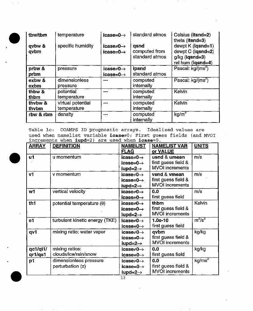
To begin any simulation, the initial conditions must be specified. The initialconditions, also referred to as the initial forecast fields, are comprised of severalCOAMPS arrays that contain values for the surface data, basic state variables andprognostic fields on each mesh. The values are given by the analysis program fromidealized user input or alternatively from real data obtained from surface databases,standard atmospheric values, first guess fields and MVOI increments. The COAMPSarrays that correspond to these initial fields are given in Tables 1 a-c.
Table la: COAMPS 2D surface arrays. Idealized values are usedwhen the appropriate namelist flag is set to 0; otherwise thedatabase values are used.ARRAY DEFINITION NAMELIST NAMELIST COAMPS
FLAG VAR, VALUE UNITS.or DATABASE
xland land/sea table ilndflg=0-> alngpct O=water;ilndfig=11- dsclim 1=land
_______________ dimensionless
zsfc terrain height itopofig=0-0 0.0 metersitopoflg=1 -4 dsclim,dsdted
psfc surface pressure itopoflg=0- psfcO Pascals:_ ~~~~kg/(MS2)
albedo albedo ialbflg=0O- albdo O=absorb;ialbflg=1 - dsclim,dsgiss 1 =reflect
dimensionlesstsea surface temperature iseaflg=0- seatmp Kelvin
iseaflg=1 -tsoil deep soil temperature -- dsclim Kelvingwet ground wetness iwetflg=0O- sfcwet O=dry; 1 =sat
iwetflg=1 -* dsclim kg/kgzO surface roughness. izOflg=0- zrough meters
izoflg=1 -4 dsclim,dsgiss
Table lb: COAMPS 3D basic state arrays. Idealized values areused when namelist variable icase•0; Standard atmospheric valuesare used when icase=0.ARRAY DEFINITION NAMELIST NAMELIST VAR COAMPS UNITS
FLAG or VALUE (NAMELIST VAR)ugeoa geostrophic u-wind icase•0,- usnd & umean m/s (iuvsnd=1)
component icase=0- ugeoa dir/spd (iuvsnd=2)geostrophic v-windcomponenttemperature
icase•0-4icase=0-4icase*0-4
12
vsnd & vmeanvgeoatsnd
m/s (iuvsnd=1)dir/spd (iuvsnd=2)Kelvin (itsnd=1)
I vgeoa
tbw/tbm
temperature
specific humidity
icase=0-
icase•0-4icase=0-4
standard atmos
qsndcomputed fromstandard atmos
Celsius (itsnd=2)theta (itsnd=3)dewpt K (iqsnd=1)dewpt C (iqsnd=2)g/kg (iqsnd=3)rel hum (iqsnd=4)
prbw & pressure icase•0-4 ipsnd Pascal: kg/(ms2)prbm icase=0-4 standard atmosexbw & dimensionless --- computed Pascal: kg/(ms2)exbm pressure internallythbw & potential --- computed Kelvinthbm temperature internallythvbw & virtual potential computed Kelvinthvbm temperature internallyrbw & rbm density computed kg/md
internally _ _ _ _
Table lc: COAMPS 3D prognostic arrays. Idealized values areused when namelist variable icase•Q; First guess fields (and MVOIincrements when iupd=2) are used when icase=O.ARRAY DEFINITION NAMELIST NAMELIST VAR UNITS
FLAG or VALUEul u momentum icase•0-> usnd & umean m/s
icase=0-> first guess field &iupd=2.-+ MVOI increments
v1 v momentum icase•0-4 vsnd & vmean m/sicase=0-- first guess field &iupd=2-> MVOI increments
W1 vertical velocity icase•0O- 0.0 m/sicase=0-4 first guess field
th1 potential temperature (0) icase0-4 thbm Kelvinicase=0- first guess field &iupd=2-~ MVOI increments
el turbulent kinetic energy (TKE) icase•0O- 1.0e-10 m0/s'icase=0-w first guess field
qvl mixing ratio: water vapor icase•0- qvbm kg/kgicase=0-4 first guess field &iupd=2-- MVOI increments
qcl/qil/ mixing ratios: icase•0- 0.0 kg/kgqrllqsl clouds/ice/rain/snow icase=0-4 first guess fieldp1 dimensionless pressure icase•0O- 0.0 kg/ms2
perturbation (7c) icase=0O- first guess field &iupd=2-- MVOI increments
13
tbw/tbm
qvbw &qvbm
Because COAMPS uses the leap-frog integration scheme, three time levels foreach of the 3D prognostic fields must be retained during each iteration. Thus, the arraynames are further identified by a time level number 1, 2, or 3:
Table 2: COAMPS array naming convention
NUMBER TIME LEVEL1 previous (t-At)
2 present (t)3 predicted (t+At)
Note that the 3D arrays shown in Table 1 c are for time level 1 representing values fromthe previous iteration. For purposes of discussion, the arrays are denoted here andthroughout the remainder of the document by the conventional notationvartl(ma(1),na(1),kka). In the code, the 3D prognostic arrays are denoted bya(ivartl(nn)), where 'a' is the forecast program array, 'i' is the pointer location forvariable 'var' at time level 'tl' on nest number 'nn'. As mentioned, the array dimensionparameters (ma(nn), na(nn),kka) correspond to the number of grid points for eachmesh that are specified by the user in the gridnl namelist. In general, all of the abovearrays, along with other fields and variables in COAMPS, are in MKS units. With thesepreliminary details in mind, the COAMPS directory structure is described below.
3.1.4. First Guess Fields and Data Assimilation
Real data initial conditions require a set of first guess fields that represent theinitial state of the atmosphere. These fields are given in one of two ways: from aNOGAPS analysis or forecast, defined as a 'NOGAPS cold start', or from a previousCOAMPS forecast, defined as a 'data assimilation update cycle'.
The NOGAPS cold start provides global fields on pressure levels and at 1 0horizontal resolution that are interpolated to the model's horizontal grid points. Thesefields are either initial conditions to the forecast program, or optionally, a first guess tothe analysis program where a multi-variate optimum interpolation (MVOI) schemeblends in observational data.
The data assimilation update cycle, shown schematically in Figure 4, begins witha NOGAPS cold start and an MVOI analysis to produce COAMPS forecast fields validone or two days prior to a particular study period. These forecast fields or 'historyfields', on the model's sigma levels and at the model's horizontal grid points, are a firstguess to the analysis program for the next COAMPS forecast. The assimilation cyclecontinues until history fields are produced for the simulation study period. Thus, themesoscale character of the flow is generated and maintained by implementing a dataassimilation update cycle.
14
0

NOGAPS Cold Start
Multivariate optimuminterpolation analysis
of NOGAPS first COMP 2 guess fields COAMPS 12 h | iCOAMPS24hi
Data Assimilation Update Cycle
Multivariate optimum interpolationanalysis of COAMPS history fields
oundaycntosupdated with
tA @¢s. :I :@ forecasts A|/ All. | /s9 . |/7 sov~jF .1 it s~sxy NOGAS 12 h)
-36 -24 -12 0 12 24tau (hr) -*.
Figure 4: Schematic representation of the COAMPS data assimilation update cycle. The procedurebegins with a 12-hour NOGAPS cold start. In this example, the cold start is initiated 36 hours beforethe initiation of the study period at tau=O h. The cold start is followed by two 12-hour data assimilationupdates using COAMPS forecast fields. A third data assimilation update initiates the 24-hour forecastfor the simulation study period. Boundary conditions during the simulation are supplied by NOGAPSforecasts every 12 hours.

3.2. COAMPS Directory Structures
The COAMPS code can be run on several different UNIX platforms including theCRAY, SGI, DEC ALPHA, and HP machines. The process for implementing COAMPSinvolves first obtaining the five COAMPS tar files. Requests for COAMPS must besubmitted to Dr. Richard Hodur, email: hodur~nrlmry.navy.mil. Also forward a copyof the request to the COAMPS system administrator Sue Chen, email:[email protected]. The five tar files are named coamps#.tar, templates.tar,database.tar, documenttar, and utilitytarwhere the '#' represents the version releasenumber.
The user first creates a ICOAMPS subdirectory and copies the COAMPS tar filesinto it. Then each of the tar files is unarchived using the UNIX command: 'tar -xvf tarfilename". Figure 5 shows the resulting directory structure obtained by performing thisstep, along with several additional subdirectories (marked with an asterisk) that areautomatically created during the process of setting up a COAMPS job.
The initial COAMPS directory contains five subdirectories comprising the entireCOAMPS system. Referring to Figure 5, these subdirectories are listed and describedbelow:
COAMPS Subdirectoriesl /coamps# - COAMPS master source codes, libraries, executables and prologues fora particular version release number given here by the '#'
IMakefile - UNIX file that creates (1) library archives of each of the codes in /libsrc,and (2) an executable by linking the libraries with the driver programs in /src
/libsrc - source codes for COAMPS librariesIMakefile - UNIX file that creates a library archive for each of the /Iibsrc codes/coampslib - subdirectory containing COAMPS source code/fishpaklib - subdirectory containing NCAR direct solvers/fnoclib - subdirectory containing FNMOC system files/nUbeqlib - subdirectory containing nonlinear balancing codeloilib - subdirectory containing multivariate optimal interpolation code
/src - source code for COAMPS driver programs/Makefile - UNIX file that creates the COAMPS executables/coampsanalysis - subdirectory containing the analysis driver program/coamps_forecast - subdirectory containing the forecast driver program/newdtg - subdirectory containing the date-time group program
/prologues - log files for describing source codes and tracking code modifications(The following additional subdirectories (flib, Ibin) are created by theMakefile in subdirectory /coamps;)
*/lib - location of library archives from each of the codes in /libsrc*/bin - location of executables for COAMPS master code
16

Figure 5: COAMPS directory structure contains five standard subdirectories: /coamps#, where # is the versionrelease number, Idatabase, Itemplates, Idocument, and /utility. These subdirectories are obtained when theCOAMPS tar files are unarchived. The two additional subdirectories, Irun and /mod are labeledwith an asterisk to indicate that they are created later by running the script file get. templates in the Itemplatessubdirectory. Similarly, the /coamps#/lib and /coamps#/bin are also created later when the user performs a"make" of the master COAMPS code in the /coamps# subdirectory.

* /Itemplates - files for generating templates to set up and run a COAMPS job/get.templates - script file for creating (1) a machine dependent run script used to
submit a COAMPS job and (2) a standardized COAMPS makefile used tocompile modified COAMPS code
/ Idatabase - COAMPS databasesImasclim - subdirectory containing global surface climatology databaseImasgiss - subdirectory containing Goddard Institute for Space Studies database/masdted - subdirectory containing 1 km terrain databaseInogaps - subdirectory containing a benchmark set of NOGAPS/adp - subdirectory containing a benchmark set of observational data
* Idocument - COAMPS documentation/Users guide -COAMPS User's Guide
/ lutility - COAMPS graphics and utility programs/Templates - script files for processing COAMPS output
(The following additional subdirectories (Imodl/emplates, frun/Templates) arecreated by the get.templates script file)
* */run - run scripts for and output from COAMPS case studies*/Templates - standardized run scripts for submitting COAMPS jobs
/run.coamps - run script template created by running get.templates* */mod - modifications to COAMPS source code
*f7emplates - standardized makefile for creating a COAMPS jobsIMakefile - makefile template created by running get.templates
Once the COAMPS directory structure has been set up, the code must becompiled. This step requires a FORTRAN 77 or FORTRAN 90 compiler for dynamicstorage allocation. In the /coamps# subdirectory, type "make machine name'. The'machine name' can be chosen from the following options:
Table 3: Standard machine settings for COAMPS compilation.MACHINE NAME DESCRIPTIONcray CRAYcray-with isis CRAY using operational database ISISsi SGI R10000sgkig SGI R10000 debug modealpha DEC ALPHAalphag DEC ALPHA debug modehp HP 9000hpg HP 9000 debug mode
This command creates the /coamps#/lib subdirectory and the COAMPS library archives(coampslib.a, fishpacklib.a, fnoclib.a, n1 beqlib.a, oilib.a) as well as the /coamps#/binsubdirectory and the master code executables (coamps analysis.exe,coampsjforecast.exe).
18
The generation of these COAMPS executables allows the user to proceed to thenext step: running a COAMPS job. This is typically accomplished by submitting aCOAMPS run script. Obtaining a run script requires running the script file get templateslocated in the /coamps#/templates subdirectory. Within this subdirectory, type"get.templates machine name" inserting the appropriate machine name from Table 3.This command prompts the user for input and upon completion, creates two newsubdirectories: subdirectory /coamps#/run/Templates containing a standardized runscript template called run.coamps, and subdirectory /coamps#/modfTemplatescontaining a standardized makefile template called Makefile. This Makefile is used tocreate updated COAMPS executables when the user modifies the original mastersource code. The procedure for modifying the master COAMPS code and submitting aCOAMPS simulation is discussed in Section 4. First, a review of the COAMPS codingframework is given in the next section.
3.3. COAMPS Code
COAMPS consists of two separate driver programs that execute the analysis andthe forecast. In the following sections, the flow chart diagrams and primary subroutinesassociated with each of these two programs are summarized and outlined.
3.3.1. Analysis
The purpose of the analysis routine coama.F is to produce a set of initialconditions for the forecast model. In addition to specifying the surface parameters andbasic state arrays, the analysis specifies 3D atmospheric fields either by interpolatingNOGAPS fields to the COAMPS grids or by blending observations with the first guessfields using the MVOI (multivariate optimum interpolation) analysis. Additionally,coama.F prepares lateral boundary conditions for the forecast model.
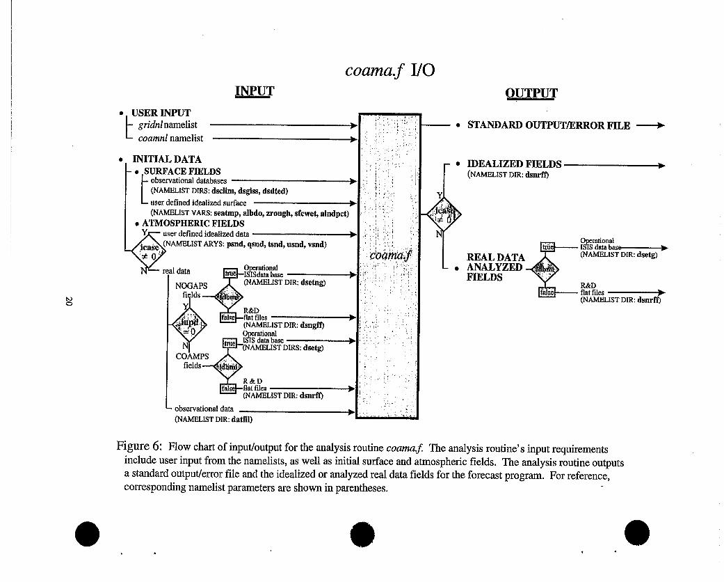
Figure 6 shows a diagram of the analysis routine's input/output including user-defined namelist values, first guess fields, and surface databases as input, and initialforecast fields as output. Each of the inputs are specified by the user to customize theinitial conditions and properly set up a COAMPS simulation. In the analysis code, thegridni namelist parameters are passed in as subroutine arguments. These parametersinclude: (1) the grid dimensioning variables, which are used later in the code to indicatedo-loop limits (ma(nn),na(nn),kka), and (2) the array allocation length nwords which isused to dimension the total analysis program array a(nwords). Additionally, the pointerlocation arrays (ivar (nn)) are dimensioned in common blocks which are incorporatedvia the include file apointers.h. Then the coamnl namelist parameters are read in tospecify model features and case study details. This namelist, containing nearly 200input variables, is the primary vehicle for the user to easily interact with the systemwithout actually making coding changes. The following information is provided to theanalysis routine through the coamnl namelist inputs:
19
coamaf 1/0
* USER INPUTgridnlnamelistcoamnI namelist
* INITIAL DATA* SURFACE FIELDSL observational databases
(NAMELIST DIRS: dsclim, dsgiss, dsdted)
user defined idealized surface(NAMELIST VARS: seatmp, albdo, zrough, sfcwet, alndpct)
* ATMOSPHERIC FIELDSYeuser defined idealized data
ty~.a~(NAMELIST ARYS: psnd, qsnd, tsnd, usnd, vsnd)
real data ? 5-ZSdlabase
NOGAPS By (NAMELIST DIR: dsetng)fi Ids
R&D>5 * -\ E~fSt files |
(NAMBLIST DIR: dsngflOperational
e ISIS data base(NAMELIST DIRS: dsetg)
COA 'MPS .fields
R&Dflat files(NAMELIST DIR: dsnrff)
- observational data >__(NAMELIST DIR: datfil)
c�wna.f
* STANDARD OUTPUT/ERROR FILE -*
0
Y
IDEALIZED FIELDS(NAMELIST DIR: dsnrff)
REAL DATAANALYZED.FIELDS
Operational-ISIS databasz(NAMELIST DIR: dsetg)
R&D- flat files --(NAMELIST DIR: dsnrft)
Figure 6: Flow chart of input/output for the analysis routine coama.f. The analysis routine's input requirementsinclude user input from the namelists, as well as initial surface and atmospheric fields. The analysis routine outputsa standard output/error file and the idealized or analyzed real data fields for the forecast program. For reference,corresponding namelist parameters are shown in parentheses.
INPUT QUTP
N)0
_
. � j
ii
t 1.i� t 41.
. :i
I .1
i
II r� i I
i
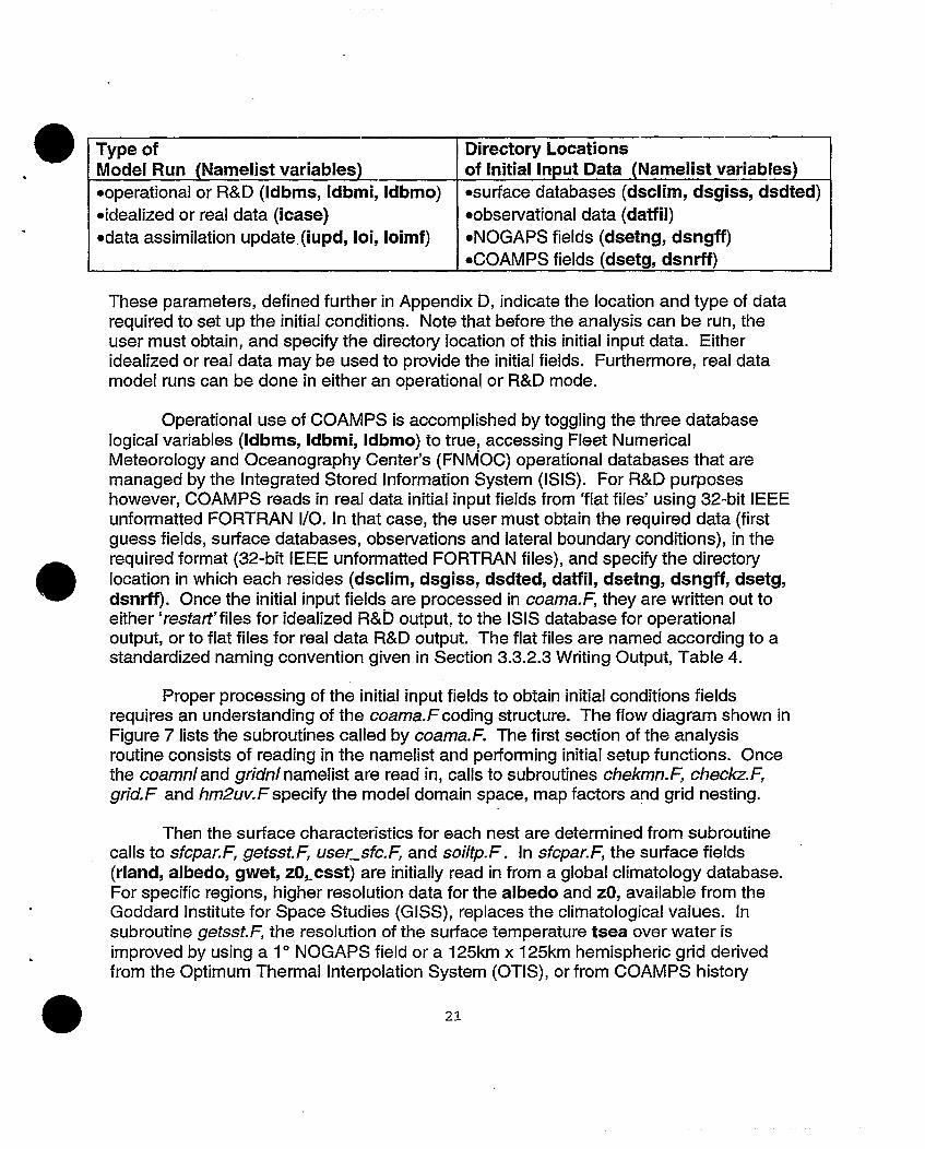
These parameters, defined further in Appendix D, indicate the location and type of datarequired to set up the initial conditions. Note that before the analysis can be run, theuser must obtain, and specify the directory location of this initial input data. Eitheridealized or real data may be used to provide the initial fields. Furthermore, real datamodel runs can be done in either an operational or R&D mode.
Operational use of COAMPS is accomplished by toggling the three databaselogical variables (Idbms, Idbmi, Idbmo) to true, accessing Fleet NumericalMeteorology and Oceanography Center's (FNMOC) operational databases that aremanaged by the Integrated Stored Information System (ISIS). For R&D purposeshowever, COAMPS reads in real data initial input fields from 'flat files' using 32-bit IEEEunformatted FORTRAN 1/0. In that case, the user must obtain the required data (firstguess fields, surface databases, observations and lateral boundary conditions), in therequired format (32-bit IEEE unformatted FORTRAN files), and specify the directorylocation in which each resides (dsclim, dsgiss, dsdted, datfil, dsetng, dsngff, dsetg,dsnrff). Once the initial input fields are processed in coama.F, they are written out toeither 'restart'files for idealized R&D output, to the ISIS database for operationaloutput, or to flat files for real data R&D output. The flat files are named according to astandardized naming convention given in Section 3.3.2.3 Writing Output, Table 4.
Proper processing of the initial input fields to obtain initial conditions fieldsrequires an understanding of the coama.Fcoding structure. The flow diagram shown inFigure 7 lists the subroutines called by coama.F. The first section of the analysisroutine consists of reading in the namelist and performing initial setup functions. Oncethe coamnl and gridnl namelist are read in, calls to subroutines chekmn.F, checkz.F,grid.F and hm2uv.Fspecify the model domain space, map factors and grid nesting.
Then the surface characteristics for each nest are determined from subroutinecalls to sfcpar.F, getsst.F, user sfc.F, and soiltp.F. In sfcpar.F, the surface fields(rland, albedo, gwet, zO~csst) are initially read in from a global climatology database.For specific regions, higher resolution data for the albedo and zO, available from theGoddard Institute for Space Studies (GISS), replaces the climatological values. Insubroutine getsst.F, the resolution of the surface temperature tsea over water isimproved by using a 10 NOGAPS field or a 125km x 125km hemispheric grid derivedfrom the Optimum Thermal Interpolation System (OTIS), or from COAMPS history
21
Type of Directory LocationsModel Run (Namelist variables) of Initial Input Data (Namelist variables)soperational or R&D (Idbms, Idbmi, Idbmo) *surface databases (dsclim, dsgiss, dsdted)eidealized or real data (icase) *observational data (datfil)*data assimilation update.(iupd, Ioi, Ioimf) eNOGAPS fields (dsetng, dsngff)
eCOAMPS fields (dsetg, dsnrff)
coama.fanalysis routine
setupparameters J�1
user inputcoamnInamelist
setup gridchekmn.f, checkz.f, grid.f, hm2uv.f:
setup model domain, map factors, grid nesting
read and process initial input fields
<caNe#
. . . . ~~~~~~~~I .
write fieldsidealized data
ioanl.f (iozavg.f, iosfcO.f,iosfctf,ioatmtf)
write idealized initial fields to'restart' files
real dataouthty.f, iosfc.f, outanl.f, outinc.fwrite surface fields, analyzed fields
and MVOI increments
I
perform multivariate optimuminterpolation analysis
oi anl.f, anlfld.f, netinc.fincorporate observations
get boundary conditionsgetbdy.f, tendbd.f, getng.f
extract coarse mesh boundary values fromNOGAPS fields for the remainder of the study
period and write out tendancies
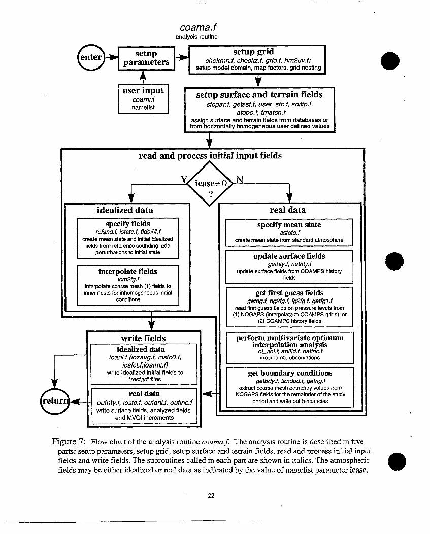
Figure 7: Flow chart of the analysis routine coama.f. The analysis routine is described in fiveparts: setup parameters, setup grid, setup surface and terrain fields, read and process initial inputfields and write fields. The subroutines called in each part are shown in italics. The atmosphericfields may be either idealized or real data as indicated by the value of namelist parameter icase.
22
I
setup surface and terrain fieldssfcpar.f, getsst.f, user sfc.f, soiltp.f,
atopo.f, tmatch.fassign surface and terrain fields from databases orfrom horizontally homogeneous user defined values
idealized dataspecify fields
refsnd.f, istate.f, flds##.fcreate mean state and initial idealizedfields from reference sounding; add
perturbations to initial state
real data
specify mean stateastate.f
create mean state from standard atmosphere
interpolate fieldsicm2fg.f
interpolate coarse mesh (1) fields toinner nests for inhomogeneous initial
conditions
update surface fieldsgethty.f, nethty.f
update surface fields from COAMPS historyfields
get first guess fieldsgetng.f, ng2fg.f, fg2fg.f, geffgl.f
read first guess fields on pressure levels from(1) NOGAPS (interpolate to COAMPS grids), or
(2) COAMPS history fields
-
r
-lop
-
-

field if either of these source are available. Otherwise, the climagological value csst isused. In subroutine soiltp.F, values for the deep soil temperature array tsoil aregenerated from climatological data. Also generated in subroutine sfcpar.F is thesurface topography field (zsfc), initialized from a 20km terrain dataset. In certainregions around the globe,1 km resolution terrain data is used for meshes with gridspacing less than 20km.
In setting up the surface characteristics of a particular case study, subroutineuser sfc.Fallows the user to customize the surface parameters with idealized valuesthrough namelist input. For example, user-defined, horizontally homogeneous valuesfor the land/sea table, surface temperature, roughness, albedo and ground wetnessarrays are given by namelist parameters alndpct, seatmp, zrough, albdo, sfewetwhen the namelist flags ilndflg, iseaflg, izOfig, ialbfig, igwtfIg are set to '0'. Thenamelist flag itopofIg when set to '0' assigns the terrain height to zero everywhere.Finally, subroutine tmatch.F matches the terrain field across the mesh boundaries andsubroutine atopo.Fcomputes the terrain gradient arrays. The coding then branches foridealized or real data initial conditions as described in the next two sections.
3.3.1.1. Idealized Data
Idealized initial conditions are typically provided by user-defined profiles of winds,temperature, pressure and moisture assumed to be horizontally homogeneous acrossthe model domain. These profiles are read in through namelist arrays usnd, vsnd,tsnd, psnd, and qsnd which are used when the namelist parameter icase is nonzero.The subroutine refsnd.F converts the initial user-defined reference sounding, into MKSunits. Then a homogeneous idealized mean state is determined from that data insubroutine istate.Ffor each of the model nests. Perturbations can be added to themean state by specifying a value for the namelist parameter icase='##'. This number'##', corresponds to a subroutine flds##.Fwhere the user assigns the fieldperturbations. When using inhomogeneous idealized fields, set the namelist parameterjcm2fg to 1 to interpolate the outer coarse mesh (1) fields to the inner nests. Thisinterpolation is done in subroutine icm2fg.F. In subroutine ioanl.F, the complete set ofidealized initial conditions (surface, basic state and prognostic fields) is written to filesthat begin with the prefix 'restart. These 'restart files become the initial forecast fieldsread in by coamm.Fto begin an idealized simulation. As discussed later, the 'restartfiles can be created at any time during the COAMPS model run and are also used toinitiate COAMPS at a nonzero forecast time (ktaust•0).
3.3.1.2. Real Data
An alternative to idealized initial input fields is the use of global or mesoscale firstguess fields that may be updated with observations. The first guess can be obtainedfrom either a NOGAPS analysis or forecast, or from a previous COAMPS forecast validat the desired date-time group (history fields).
23
First, the basic state profiles are specified through subroutine astate.F. Thenthe previously specified surface parameters are replaced with higher resolutionCOAMPS history fields, if they are available. From calls to gethty.Fand nethty.F, the2D arrays for surface parameters on each nest are updated if the logical namelistparameter Inrhty=.true.. These fields (gwet, zO, tsea), initially read in from a globalclimatology database, are assigned values given by the COAMPS history fields. Whilethe array for snow coverage (snow) is given values from the NOGAPS global field, theother 2D surface fields obtain values from the COAMPS history fields. These fieldsinclude: the lOm winds (ulOm, viOm), boundary layer depth (blht), surface fluxes(hflxs, hfIxl) and wind stress (stres). When lnrhty=.false., or if history fields are notfound, this latter set of fields are set to zero initially.
The procedure for obtaining the first guess fields begins with subroutine getng.Fthat reads in NOGAPS fields for:
* surface pressure* u- and v-momentum* geopotential heights* vapor pressure
These fields are specified at 10 horizontal resolution and at pressure levels pr(lm),where Im and pr are user defined namelist parameters defined further in Appendix D.The fields are then interpolated to the coarse mesh (1) grid points in subroutine 0ng2fg.F Subroutine fg2fg.Fperforms the interpolation of the coarse mesh (1) to theinner nests. If a previous COAMPS forecast is available and the proper namelist flag isset (iupd•0), then subroutine getfgl.F is called to overwrite the above fields withCOAMPS history fields for each nest. Both routines getng.Fand geffgl.Fsearchbackward through seven date-time groups in an attempt to provide COAMPS with themost recent data.
Finally, the first guess fields are adjusted based upon observational data via amultivariate optimum interpolation (MVOI) analysis performed in the subroutine oianl.F(loi=.true.). Note that the MVOI analysis subroutines are not stored with the rest of theCOAMPS source code (See Section 3.2, and Figure 5), but are contained in a separatesubdirectory and compiled into a separate library. The oi anl.Fsubroutine determinesheight and momentum increments based upon differences between the first guessfields on the coarse mesh (1) and ADP observations (i.e. rawinsonde, SSMI, satellitederived data, etc.). These increments are added to the first guess fields and a 9-pointsmoother is applied in subroutine anffid.F. The same procedure can be used to obtainMVOI increments directly on the inner nest first guess fields (loimf=.true.). Alternatively(loimf=.false.), the coarse mesh (1) MVOI increments can be interpolated to the innernest grids and then added to the inner nest first guess fields using subroutine netinc.F;however, this procedure is less effective at maintaining the mesoscale structure of theobservations. Using a Cressman scheme, additional analyses are also available on the _
24

pressure levels for temperature (Itanl=.true.) and dew point depression (Iqanl=.true.),as well as for surface temperature (Itanls=.true.).
To produce a forecast from real data, boundary conditions for the prognosticfields must be supplied to the coarse mesh (1) at a given time interval (itauin). For aspecified forecast length (itauf), the boundary values are extracted from the NOGAPSforecast fields in subroutine getbdy.F, and the tendencies are computed and written outin subroutine tendbd.F, again following the standard naming convention.
The final set of real data initial conditions is written out by three outputsubroutines. Subroutines outhty.F, iosfc.Fwrite out the surface fields while subroutineoutanL.Fwrites out the analyzed fields at the pr(lm) pressure levels. For use in dataassimilation, subroutine outinc.F writes out the MVOI increments (loi=.true.). Since thebasic state arrays are easily recomputed, they are not written out by the analysisroutine for real data cases. The files created by the analysis are named following thestandard convention described in Section 3.3.2.3 for which each filename begins with afour character prefix identifying the field of data it contains. This completes the codingstructure associated with the analysis subroutine coama.Fand the preparation ofCOAMPS analyzed fields.
3.3.2. Forecast
The purpose of the coamm.F code is to produce predicted values of the time-dependent variables. Associated input/output tasks include reading in the initialconditions and writing out the model results. These I/O functions are shown in Figure 8.As in the analysis routine, first the gridnl namelist parameters, passed in as subroutinearguments, are used to indicate do-loop limits (ma(nn),na(nn),kka), and the arrayallocation length nwords is used to dimension the total forecast program arraya(nwords). Additionally, the pointer location arrays are dimensioned in common blockswhich are incorporated via the include file mpointers.h. Then the coamnl namelistparameters are read in to indicate model features and case study details specified bythe user. The 2D graphics instructions, designated here by filenames 'ocards' and'xcards', are read in so that the proper output fields will be saved for graphical display.Finally, the analysis fields created by coama.F are input from either the 'restart'files,ISIS database, or R&D flat files. The forecast routine produces output at specified timeintervals for evaluation of model results. COAMPS output includes a standardoutput/error file, and additional output as requested by the user: 'restart files, 1 D, 2Dand 3D graphics files.
With an understanding of the forecast routines I/O, the coamm.Fcoding isdescribed below. The forecast is produced by integrating a set of model equationsgoverning the prognostic nature of each time-dependent variable. Where necessary to
25

coamm.f 1/0
* USER INPUT- gridni namelist -- coamnl namelist- ocards- xcards
* ANALYSIS FIELDSy idealized data
(NAMELIST DIR: dsnrff)
~4'at ~ y restart data; (NAMELIST DIR: dsnrff)
N lo~~OerationalN ~~~~~~~IS Sdata base(NAMELIST DIR: dsetg)
real data
R&D __ _ _ _ _
fals flat files(NAMELIST DIR: dsnrff)
N,0M
.l . ! .
II
* STANDARD OUTPUT/ERROR FILE -*
0
OperationalISIS data bas (NAMEUST DIR: dsetg)
R&Dflat files -(NAMELIST DIR: dsnrff)
IDFORECASTDATA(NAMELIST DIR: dsetld)
* RESTART FILESy restart files
(,+AMELIST DIR: dsnrff)
Figure 8: Flow chart of input/output for the forecast routine coamm.f. The forecast routine uses from the
coamnl namelist, input parameters icase to setup idealized or real data, ktaust to determine if 'restart' files
or if the analysis' first guess fields are input, and Idbms to access the operational database or R & Dflat files. The coamnl namelist also assigns the directory locations, shown in parentheses, of data input/output.
The files ocards and xcards contain user-specified graphics directives. For reference, corresponding namelist
parameters are shown in parentheses.
*~~
INPUT OUTPUT
I.
close the system of equations or to represent certain processes, physicalparameterizations have been utilized. The following section discusses the codingstructure and subroutine calls within subroutine coamm.F. Aside from initial setupfunctions performed by the subroutine, it is subdivided into two other parts: reading ininitial conditions and performing the forecast. While reviewing this section, refer to theflow chart and subroutines shown n Figure 9.
3.3.2.1. Reading Initial Conditions
Subroutine coamm.F begins by reading in the coamnl namelist to allow for user-defined model input and then performs several setup functions that initialize and defineconstants, parameters, variables and arrays used later in the forecast routine.Additional setup code is embedded in subroutine coami.F: the model domain space,map factors and grid nesting are determined from routines grid.F, hm2uv.F, and 2Dgraphics instructions are read in from routines reado.F, readx.F. Then, the assignmentof COAMPS initial forecast fields is done in coami.F. If idealized data (icase•O) areused or a restart run is initiated (ktaust#0), subroutine iomdl.F is called to open the'restart files to provide the initial conditions. Otherwise, real data initial conditions areobtained from subroutine calls to insfc.F, atopo.F, astate.F, inIvl.F.
When using real data, subroutine inlvl.Fspecifies the initial forecast fields basedupon the type of data assimilation select by the namelist parameter iupd. Wheniupd=0, a NOGAPS cold start is performed by interpolating analyzed NOGAPS fieldson pressure levels to COAMPS sigma levels and horizontal grid points. When iupd=1,a full COAMPS update is performed by interpolating the analyzed COAMPS fields onpressure levels to sigma levels (subroutines instdp.F, stdp2z.F). When iupd=2, anincremental update is performed in subroutine incrup.F, where the COAMPS historyfields on model sigma levels and the MVOI increments on pressure levels are read in.After the increments are interpolated to the model sigma levels, variational adjustmentsare made on the pressure and potential temperature increments to bring the fields intohydrostatic balance and then the increments are added to the COAMPS forecast.
Returning back to subroutine coami.F, next a few additional preliminary steps aretaken before performing the model forecast. Boundary values are extracted insubroutines readbd.Fand tendbd.F, and several model parameters are computed usingnamelist input. For example, lateral boundaries and weighting functions are determinedfrom kgetbc, ibdya, jbdya; the mixing length array is defined using iamxgl; the spongelayer is specified by Iralee, Ispong, nrdamp; and the diffusion coefficients aredetermined from dif4th anid dif2nd. In addition, the prognostic fields are broadcast tothe other time levels in asetup.F. If the logical variable linit=.true., subroutine ainit.F isused to modify or update certain fields used by the model. (Each of these user-specified parameters are further defined in Appendix D.) Finally, the initial forecastfields are written out by subroutine output.F.
27

coamm.fforecast routine
setup gridchekmn.f, checkz.f, coami.f (grid.f, hm2uv.f):setup model domain, map factors, grid nesting
I
user inputcoamninamelist
rea(
setup 2D outputcoami.f (reado.f, readx.f): read in and setup 2Dhorizontal and vertical slice output directives
I
coami.
read from 'restart' files iomdl.f (iozavg.f, iosfcO.f, iosfct.f, ioatmtf):initialize sfc, mean state and 3D fields fromidealized data or from a model restart
read real dataI insfc.f, atopo.f, astateAf initialize sfc and basic stat I
2inIvlI.f initialize 3D fields on sigma levels
I instdp.h read analyzed pressure level fields
incrup.f add MVOI increments to sigma iUpdlevel fields; do variational adiustmentfstdp2zAf interpolate pressure level fieldsto sigma levels; do variational adjustment
28
setup and write fieldsasetup.f, aint.f, readbd.f, tendbd.f, output.broadcast initial fields to other time levels,initialize vertical velocity, compute boundarytendencies and output initial fields.
~~*1~A
bounda[ies
Yi perform forecast (iterl=iterls,itere(l): ktaust ktauf, delta) I-
I readbd.f. real data coarse nest boundaries I
i write forecast data_ outputf (aprintf, outsfc.f, aoutp.f, aoutz.f,
nest loop (nn=1,nnest) aoutxz.f, asavld.f, iosig.f, visout.f): writeamodeLf: coarse nest integration quick print data to standard output, 1 D, 2D and
00, bdrf, mbdy.h real data inner nest - 3D fields to output files (See Figure 11)
4
I1write to 'restart' files
iomdl.f (iozavg.f, iosfcO.f, iosfct.f,ioatmt.f): save model fields
I
I
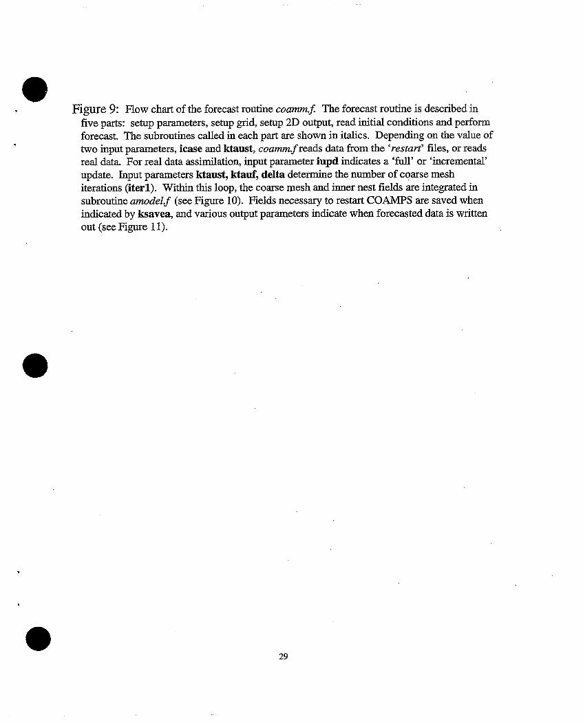
Figure 9: Flow chart of the forecast routine coamm.f The forecast routine is described infive parts: setup parameters, setup grid, setup 2D output, read initial conditions and performforecast. The subroutines called in each part are shown in italics. Depending on the value oftwo input parameters, icase and ktaust, coammf reads data from the 'restart' files, or readsreal data. For real data assimilation, input parameter iupd indicates a 'full' or 'incremental'update. Input parameters ktaust, ktauf, delta determine the number of coarse meshiterations (iterl). Within this loop, the coarse mesh and inner nest fields are integrated insubroutine amodel.f (see Figure 10). Fields necessary to restart COAMPS are saved whenindicated by ksavea, and various output parameters indicate when forecasted data is writtenout (see Figure 11).
29
At this point, control returns to the main forecast subroutine coamm.F. And sinceall model arrays, variables and parameters have been assigned values, COAMPS isnow ready to begin integration of the initial forecast fields.
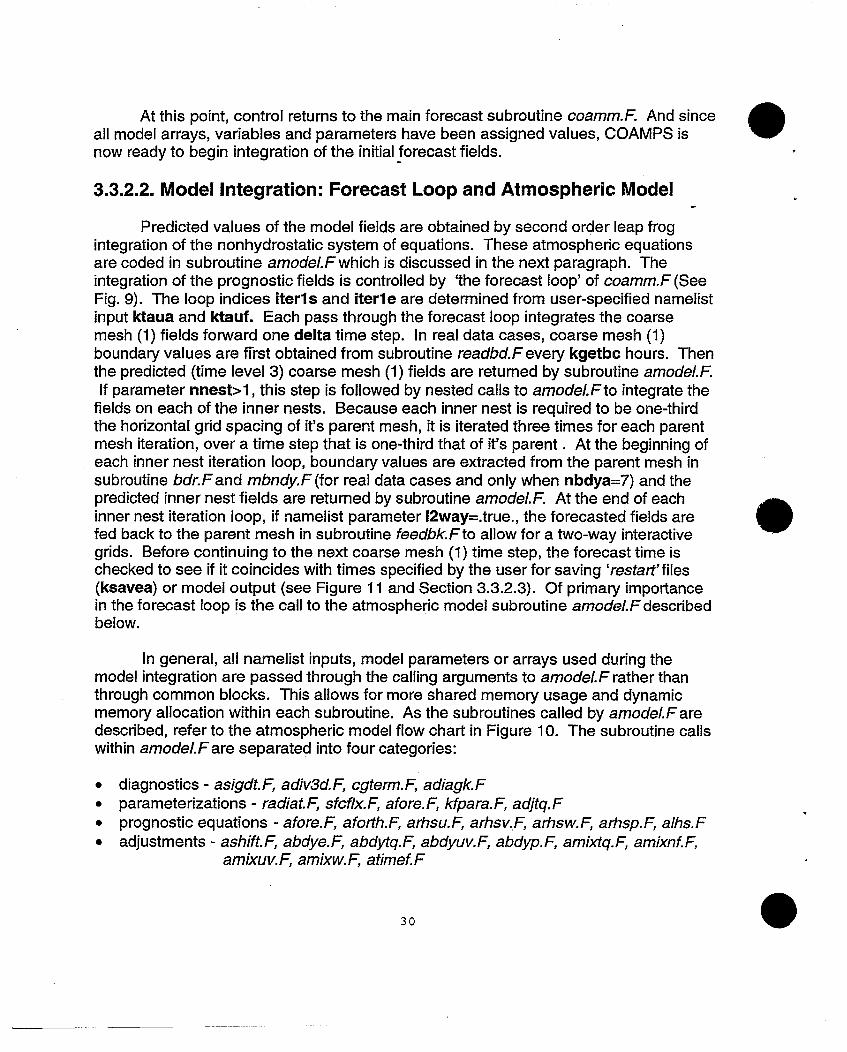
3.3.2.2. Model Integration: Forecast Loop and Atmospheric Model
Predicted values of the model fields are obtained by second order leap frogintegration of the nonhydrostatic system of equations. These atmospheric equationsare coded in subroutine amodeLFwhich is discussed in the next paragraph. Theintegration of the prognostic fields is controlled by 'the forecast loop' of coamm.F (SeeFig. 9). The loop indices iterls and iterle are determined from user-specified namelistinput ktaua and ktauf. Each pass through the forecast loop integrates the coarsemesh (1) fields forward one delta time step. In real data cases, coarse mesh (1)boundary values are ffrst obtained from subroutine readbd.Fevery kgetbc hours. Thenthe predicted (time level 3) coarse mesh (1) fields are returned by subroutine amodel.F.If parameter nnest>1, this step is followed by nested calls to amodel.Fto integrate the
fields on each of the inner nests. Because each inner nest is required to be one-thirdthe horizontal grid spacing of it's parent mesh, it is iterated three times for each parentmesh iteration, over a time step that is one-third that of it's parent . At the beginning ofeach inner nest iteration loop, boundary values are extracted from the parent mesh insubroutine bdr.F and mbndy.F (for real data cases and only when nbdya=7) and thepredicted inner nest fields. are returned by subroutine amodel.F. At the end of eachinner nest iteration loop, if namelist parameter 12way=.true., the forecasted fields arefed back to the parent mesh in subroutine feedbk.Fto allow for a two-way interactivegrids. Before continuing to the next coarse mesh (1) time step, the forecast time ischecked to see if it coincides with times specified by the user for saving 'restart'files(ksavea) or model output (see Figure 11 and Section 3.3.2.3). Of primary importancein the forecast loop is the call to the atmospheric model subroutine amodel.Fdescribedbelow.
In general, all namelist inputs, model parameters or arrays used during themodel integration are passed through the calling arguments to amodel.F rather thanthrough common blocks. This allows for more shared memory usage and dynamicmemory allocation within each subroutine. As the subroutines called by amodel.F aredescribed, refer to the atmospheric model flow chart in Figure 10. The subroutine callswithin amodeLFare separated into four categories:
* diagnostics - asigdt.F, adiv3d.F, cgterm.F, adiagk.F* parameterizations - radiat.F, sfcflx.F, afore.F, kfpara.F, adjftq.F* prognostic equations - afore.F, aforth.F, arhsu.F, arhsv.F, arhsw.F, arhsp.F, alhs.F* adjustments - ashift.F, abdye.F, abdytq.F, abdyuv.F, abdyp.F, amixtq.F, amixnf.F,
amixuv.F, amixw.F, afimef.F
30

amodel.fatmospheric model equations
and parameterizations
enter ~~~ashiftff (adj): shift time level arrays to prepare for the next iteration
(el, th1, qvi, qco, qrt, qi1, qsv, a vel, o w o, p1,e2, th, qv2, qc2, qr2, qi2, qs2, u2, v2, w2, p2,e3, th3, qv3, qc3, qr3, qi3, qs3, u3, v3, w3, p3)
|asigdtff (diag): compute the vertical velocity associated with the|model coordinates for time level 2 (sigdt)
adiagk.f (diag): computethe Smagorinsky eddy mixingcoefficientarray (eks)
rh sUfx.f (para): compute the\Y ~~~~surface fluxes and stressesx . ~~~~(hfluxl, hfluxs, stresx, stresy)
t afore.f (para/prog): predict tendencies and update the turbulent kinetic energy)
4 aorths.f (prog): predictadetemoetendenciesfoforoen athem veraticral eoiy (t rhs)
aforqx.f (prog): predict\ ? / ~~~tendencies of cloud and rain
\/ ~~~~mixing ratios (qc3, qr3)
abdq.f (prog): predict tendencies of ice and snow mixing ratios (qi3, qs3) 1
se ;,~~3 afoq (prog): predict tendencies of water vapor mixing ratio (qv3)I
arsf (prog): predict advective mode tendencies for the U-momentumn (urhs)|
| arsv~f(prg): predict advective mode tendencies for the v-momentumn (vrhs|
rarhsw.f (prog): predict advective mode tendencies for the vertical velocity (wrhs)
arhsp.f (prog): predict advective mode tendencies for the pressure (prhs) I
abdye. f, abdytq. f (adj): apply boundary conditions (e3, qc3, qi3, qr3, qs3, qv3, th3)|
asigdt.f (diag): compute the vertical velocity associated with themodel coordinates for time level 2 (sigdt)
(continued)
31
adiv3d.f (diag): computethe 3D divergence array(div3)
cgterm.f (diag): computethe counter gradient terms(th3, qv3)
I,(continued)
L-..iter2=1,ktaua: mtaua 4alhs.f (prog/adj): predict the fast mode tendencies for the pressure,vertical velocity and momentum terms, update the u-momentum (u3),v-momentum (v3), vertical velocity (w3), pressure (p3),and potentialtemperature (th3), apply boundary conditions (th3, p3, u3, v3, w3)
*adTra d update th3 with the radiational heating rate tendencies (trad)
abdye.f, abdytq.f, abdyuv.f (adj): apply boundary conditions(e3, th3, qv3, qc3, qr3, qi3, qs3, u3, v3, w3
k amixtqf (pam): implicit vertical mixing (th3, qv3)
9 amixnf f(para): implicit vertical mixing (.3)
1 amixuv.f (para): implicit vertical mixing (u3, v3)
q amixwff (para): implicit vertical mixing (w3)
Lvertical mixing (qc3, qr3)1
abdye.f, abdytq.f, abdyuv.f (adj): apply boundary conditions(e3, th3, qv3, qc3, qr3, qi3, qs3, u3, v3, w3
kfpara.f (para): compute convective tendencies (qc3, qr3, qv3, th3)
I adjtq.f (para): compute the microphysical tendencies (th3, qv3, qc3, qi3, qr3, qs3)
I radiatf (para): compute radiative heating rate tendencies (trad)
I abdytq.f (adj): apply boundary conditions (th3, qv3, qc3, qi3, qr3, qs3) I
32
atimef.f (adj): filter high-frequency temporal oscillations(e2, p2, qc2, qi2, qr2, qs2, qv2, th2, u2, v2, w2)

Figure 10: Flow chart of the atmospheric model subroutine amodel.f. Subroutines calledby amodelf are designated as: adjustment (adj), diagnostic (diag), prognostic (prog), and/orparameterization (para) routines. Shown in parentheses are the arrays updated in eachsubroutinecalled by amodel.f. The number associated with each array indicates the timelevel. Many of the model parameterization features are controlled by input parameters. Forexample, subgrid scale mixing is controlled by parameters Itke, iamxgl, iahsgin, surfacefluxes by Iflux, thermodynamic processes by Imoist, lice, convective parameterization byIcupar, dftueso, and radiative affects by Irad and the internal logical parameter lupradwhich obtains a value based upon the values of both Irad and dtrad. See Appendix D for amore thorough description of these, and the other COAMPS namelist input parameters.
33

Within amodel.F, first the time levels associated with the prognostic arrays areshifted in subroutine ashift.Fto prepare them for the next model iteration. Toillustrate this process, we use the u-momentum component array as an example:
ul(m,n,kk) = u2(m,n,kk)u2(m,n,kk) = u3(m,n,kk)u3(m,n,kk) = ul(m,n,kk).
After ashift.F, time level 1 arrays contain previous values (time=t-At), time level 2 arrayscontain present values (time=t), and by the end of amodel.F, time level 3 arrays containpredicted values (time=t+At). Note that the array dimensions used in amodelFaremore general (m,n,kk) since they can represent the dimensions of any mesh.
Before the prognostic tendencies are computed, several preliminary diagnosticroutines are called to define arrays used later. These routines include: asigdt.Fwhichcomputes sigma-coordinate vertical velocities (sigdt), adiv3d.Fwhich computes the twoor three-dimensional divergence (div3), cgterm.Fwhich computes and adds in countergradient flux terms to the potential temperature and water vapor mixing ratio wheniamxgl=4 or 5, and adiagk.Fwhich computes Smagorinsky type horizontal eddy mixingcoefficients when iahsgm=1 (eks). The surface parametertization routine, sfcflx.F, isalso called in advance to produce values for the surface fluxes (hfluxl, hfluxs) andstresses (stresx, stresy) used as lower boundary conditions for the water vapor,potential temperature and wind components respectively.
Next, the predicted future values of the time dependent variables are obtained.The terms associated with the slow or advective modes in COAMPS are computed firstin subroutines afore.F(e3), aforth.F(thrhs), aforqx.F(qc3, qi3, qr3, qs3, qv3), arhsu.F(urhs), arhsv.F(vrhs), arhsw.F(wrhs), and arhsp.F(prhs). In the above routines,
time level 3 arrays for TKE and moisture are updated because they do not containterms related to the faster moving sound and gravity waves which are computedseparately. The forcing associated with the fast modes are integrated in subroutinealhs.F using a time-splitting and semi-implicit computation over a shorter time stepdetermined from namelist variable mtaua. Here the time level 3 arrays for the potentialtemperature, wind components and pressure are updated adding in the previouslycomputed advective mode tendencies (thrhs, urhs, vrhs, wrhs and prhs).
Once the time level 3 arrays have been updated, adjustments are made to theprognostic variables. These adjustments include explicit moist physics, radiation,turbulent vertical mixing, and temporal filtering. For example, subroutine kfpara.Fcomprises a convection parameterization scheme used when the logical variableIcupar=.true. and when the horizontal resolution of the nest is greater than thatspecified by namelist parameter dxmeso. Subroutine adjtq.F is a cloud microphysicalparameterization scheme that handles subgrid scale moisture processes whenImoist=.true.. Subroutine radiaf.Fparameterizes the long and short wave radiation
34

effects upon the potential temperature when logical variable lrad=.true.. Also listed asa parameterization subroutine is the TKE prediction routine afore.F called whenItke=.true.. This routine consists of 1.5 order boundary layer closure with severaloptions for parameterizing the eddy mixing coefficients and the turbulent mixing length.
Further adjustments are made to the time level 3 arrays by applying boundaryconditions, in subroutines abdye.F, abdytq.F, abdyt.F, abdyuv.F, abdyw.F, abdyp.F,and performing vertical mixing, in subroutines amixtq.F, amixnf.F, amixuv.F, amixw.F(Itke=.true.). Finally, temporal oscillations associated with the leap frog integrationscheme are smoothed in subroutine atimef.F. To maintain numerical stability, thedamping, diffusion, filtering and horizontal mixing computations are performed on thetime level 1 arrays, and vertical mixing is done implicitly on the time level 3 arrays. Allother quantities are computed on time level 2 arrays. See Section 2 for a list ofreferences that describe the parameterization and adjustment schemes used inCOAMPS, and Appendix D for further descriptions of the namelist input parameters.
The coding in the above subroutines completes one model iteration with updatedpredicted values stored in the time level 3 arrays. Control returns to the forecast routinewhere the atmospheric model is called for up to six additional inner nests, thusrepeating the amodel.Fcoding sequence. At the end of each coarse mesh (1) iteration,coamm.F queries whether the forecast fields are written to 'restart files (in subroutineiomdl.F) and/or graphical display files (in subroutine output.F) as described in the nextsection.
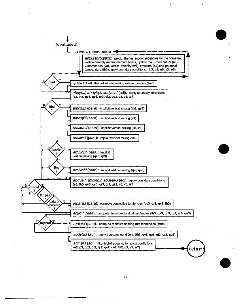
3.3.2.3. Writing Output
COAMPS produces several forms of model output in subroutine output.Fforviewing case study results and testing code development. Output options include: 2Dhorizontal and vertical slices of data viewed in numerical format, called 'quick prints', aswell as 1 D, 2D, and 3D data post-processed through a variety of separate graphicsprograms. Figure 11 depicts the flow diagram for writing out COAMPS results. Here,the subroutines are briefly introduced beginning with an overview of 2D data output.More detailed information concerning COAMPS graphics is presented in a separatedocument.
In subroutine aprint.F, a predetermined set of model fields is written to standardoutput in 2D numerical quick print format at time intervals specified by the user(kprnta). The standard output file also contains standard error messages, and thus, inaddition to numerical output of model fields, also indicates if the job has completedsuccessfully. The 2D horizontal and vertical slice data, generated for graphical displaypurposes, are specified by the user before a COAMPS model run. This information isread into COAMPS through graphics 'directives' given in files whose names correspondto the input parameters npfil (horizontal slice data) and xsfil (vertical slice data).
35
output.fwrite forecast data
Figure 11: Flow chart of the subroutines called by coamm.f that write out model data. The
input parameters kprnta, tid, ksaves, tvis represent forecast times, defined in AppendixD, that are converted into iteration numbers,. The ocards and xcards iterations refer totimes given in the 2D graphics directive files created by the user.
36

The 2D graphics directives are used in subroutines outsfc.F, aoutp.F, aoutz.F, andaoutxz.F, to produce the following types of output:
. outsfc.F- surface fields* aoutp.F - horizontal slices of fields at pressure levels* aoutz.F - horizontal slices of fields at height levels* aoutxz.F- vertical slices of fields
The output files generated are named following a standardized naming convention.Each unique filename uses 36 characters to identify 11 pieces of information about thedata it contains. For example, filename wspda2199406081200600000002000000hsIrepresents:
The filename indicates that the data are of horizontal wind speed from the atmosphericmodel on the second nest. Furthermore, the data are a horizontal slice on a heightsurface at a height of 20 m, 6 hours into a forecast initialized at 12Z on June 8th, 1994.Table 4 summarizes the information given by the output filename.
Table 4: COAMPS Output File Naming ConventionOUTPUT FILENAME TYPE POSITION OPTIONS-DESCRIPTIONfield name indicator a4 1-4 see COAMPS graphics documentmodel type indicator al 5 a - atmosphere
.____________________ o - oceannest number indicator i .1 6 1 - coarse mesh
.____________________ 2,3,4,5,6 or 7 inner nestsdate-time group a10 7-16 YYYYMMDDHHforecast time: hr i3.3 17-19 a time within the forecast period
min i2.2 20-21 evenly divisible by the time stepsec i2.2 22-23
level: meters i5.5 24-28 height level (horizontal slice data)second level: meters i5.5 29-33 2n" height level (for thickness fields)level type indicator a2 34-35 sl - mean sea level
hs - height surfaceml- marine levelsf - surfacepr - pressure level
plot type indicator al 36 I - horizontal sliceI x - vertical slice
37

Subroutines for producing 1 D (grid point) and 3D volumes of model data, arebriefly mentioned here. The 1 D data output is determined from the coamnl namelistvariables tld, dsetld, cpar, city, ild and jld. Subroutine asavld.Fcreates lDgraphics files (with filename prefix 'tsef) at time intervals given by tid. And subroutineiosig.Fcreates 3D volumes of sigma level data (with the filename ending in 'sgt) and2D surface data (with the filename ending in 'sff) at time intervals given by two namelistparameters: icycle (for use in data assimilation) and ksaves (for graphical display:Viz5d, GrADS). The standard set of output produced by this subroutine is listed inTable 5 for reference.
Table 5: Sigma level data and surface fields written out byCOAMPS
:3D Volumes ....... 2D Surface Fieldspressure (Pascals) ground wetness (fraction)perturbation pressure (Pascals) ground/sea surface temperature (K)potential temperature (K) boundary layer height (m)u-momentum component (m/s) sensible heat flux (W/m**2)v-momentum component (m/s) latent heat flux (W/m**2)water vapor mixing ratio (kg/kg) wind stress (Newton/m**2)cloud water mixing ratio (kg/kg)ice crystal mixing ratio (kg/kg)rain drop Mixing ratio (kg/kg)snow flake mixing ratio (kg/kg)turbulent kinetic energy (m**2/s**2)vertical velocity (rn/s) _
Another option is available for viewing primarily 2D model results using thegraphics package VisuaL Subroutine visoutFcreates Visualfiles (with the filenameending in 'GRD1', GRDZ, or GRDG') at time intervals given by namelist inputs tvisl,tvis2.
This completes the overview of the COAMPS code. At this point, the flowstructure of the code, the subroutine functions, and the use of certain namelistparameters have been described. In the next section, the procedure for submitting aCOAMPS job is reviewed.
38

4. Execution Procedure
The execution procedure for a COAMPS job involves two phases: case studysetup and submitting a COAMPS job. Before a COAMPS job begins, severalpreliminary steps are taken involving preparation of the initial conditions and the code.The steps outlined below show how to get started using COAMPS as a new user, andhow to set up a new case study. First time users of COAMPS, need to obtain theCOAMPS tar files, set up the COAMPS directory structure and compile. the masterCOAMPS libraries and executables. These steps are covered in Section 3.2. Alsodescribed in Section 3.2 are the steps for obtaining two templates: a run script used torun the COAMPS executables, run.coamps, and a makefile used to create modifiedexecutables, Makeffile. The steps given here describe how to run a user-customizedCOAMPS simulation with the option of modifying the original source code.
4.1. Preparation Steps
CODE MODIFICATIONS(To run unmodified source code, goto step 10.)
1. cd to the subdirectory Icoamps/mod2. type "mkdir modsd' where modsd is any user-defined subdirectory name that will
contain user generated code modifications3. cd to this new subdirectory modsd4. type "cp .J/Templates/Makefile ." to get the Makefile template into the 'modsd
subdirectory.5. copy subroutines from any of the subdirectories in /coamps#/libsrc for modification6. modify and add subroutines7. copy all include files (*.h) from the subdirectories in /coamps#/libsrc that are called
by the subroutines that have been modified8. edit the Makefile to include object files corresponding to subroutines that have been
modified or added9. make the new executable: type "make machine namd' (See Table 3)
INITIAL INPUT FIELDS10. obtain the initial input fields
* <real data case>To perform a NOGAPS 'cold start', COAMPS uses 10 resolution NOGAPSfields in flat file format (32-bit, IEEE) and ADP observational data in FGGEformat. These data are available from FNMOC and can be obtained using ananonymous ftp. For a typical model run, a NOGAPS analysis or forecastprovides the first guess fields and 12 hourly NOGAPS forecasts provideboundary conditions throughout the duration of the simulation study period.In the absence of NOGAPS forecasts, fixed boundary conditions are used(although this is not recommended). Once these data are obtained, theyshould be copied into the appropriate subdirectory:
39
/coamps#/database/nogaps and /coamps#/database/adp. Other databasesused in COAMPS (surface fields, terrain characteristics and climatology data)are provided with the initial COAMPS tar file database.tar. These data arealso required to be in flat file format. (Note that the subdirectory locations ofthis initial input data must be provided as namelist input: parameters dsngff,dsclim, dsdted, dsgiss.)<idealized case>Obtain or create an idealized sounding (pressure, temperature, moisture andwinds) and input these data through namelist arrays psnd, tsnd, qsnd usnd,vsnd. Perturbations, used to modify these initial idealized profiles, may bedefined by the user in subroutine flds##.F. Perturbations are added whenthe namelist parameter icase=## coincides with the number in the flds##.Ffilename. The surface fields can be defined from either user-specifiednamelist parameters: alndpct, seatmp, zrough, albdo, sfcwet or from thestandard COAMPS surface databases located in subdirectory/coamps#/database. (Note that if real surface data is used, the subdirectorylocations of the surface databases must be provided as namelist input:parameters dsclim, dsdted, dsgiss.)
CASE STUDY11 .cd to the subdirectory Icoamps/run12. type "'mkdir runsd' where runsd is any user-defined directory name that will contain
a case study run script and output files13. cd to this new subdirectory runsd14.type 'cp .JTemplates/run.coamps .' to get the COAMPS run script template into
the runsd subdirectory.15. edit the run.coamps run script to customize the namelist input for a particular case
study (i.e. modify the gridnl, coamnl, and mvoinl namelists (See Section 4.2))16. if the COAMPS executables have been modified, make sure that the binDir
variable in the run.coamps script points to the location of the new executables.17. create a /coamps/data subdirectory for graphical and model output data
These steps summarize the preparation phase of a COAMPS job. Correctspecification of user input (step 15) is of primary importance in the above sequence.Because COAMPS includes a variety of important features and options as namelistinput, the user has the ability to interact with the code through these namelists.Although this is of great benefit, high levels of user input also creates the opportunity forerror. To educate the user and reduce the risk of error, categories of user input aregrouped below based upon their function with the COAMPS system.
40

4.2. COAMPS Input File: Gridni, Coamni and Mvoinl Namelists
Perhaps the single most important step in running COAMPS successfully isindicating the proper namelist input. Many of the more important model parameters arespecified by the user in the three model namelists gridnl, coamnl and mvoinl. Theparameters from these namelist and their user-specified values are assigned in a singleinput file which, for purposes of discussion, is called nfistinput. This input file is createdwhen the COAMPS run script is submitted (See Appendix B for a sample input file). Acomplete list of the namelist input parameters, default values, and definitions is given inAppendices C and D arranged alphabetically according to the type of input (i.e. integer,real, character, logical). Categories of user inputs described here include the followingparameter groups: model setup, case study setup, and data manipulation.
4.2.1. Model Setup
This section describes the inputs that allow the user to set up the model domainand grid structure, the integration procedure, and the boundary conditions for aparticular case study.
4.2.1.1. Grid
Specification of the namelist parameters associated with the grid setup arecritical in producing a proper model run. Their values vary from case to case dependingon the region/domain of interest, and the vertical/horizontal spacing required to resolvemeteorological features of interest.
Input parameters:the number of nests nnest; horizontal grid spacing of the coarse mesh delx, dely;vertical grid spacing dsigma; number of grid points for each nest ma(nn), na(nn), kka;map projection nproj; standard latitude(s) and longitude phntl, phnt2, alnnt; referencelatitude and longitude rlat, rlong; reference grid points iref(l), jref(l); reference gridpoints of inner nests ii(nn), jj(nn) (where nn is the nest number)
It is possible to determining the model domain in advance of a COAMPS job byrunning the script file domain.sh located in the lutility! Templates subdirectory. Edit thisfile, inputting values for the grid setup parameters, and then type: "domain.sh". A metafile of the nested model domain is created and displayed on the screen, provided thatthe DISPLAY environmental variable has been specified and the 2D graphicsexecutable plotxy is available. Once you are satisfied with the model domain, insertthose parameter values into the coamnl namelist. Examples of three model domainsare given in Appendix E. Tables E-1 ,E-2,E-3 give the namelist parameter values usedto set up a model grid based upon the mercator, lambert conformal, and polarstereographic map projections respectively. Figures E-2,E-4,E-6 show the
41

corresponding COAMPS model domains obtained by running domain.sh script for eachof the three examples.
4.2.1.2. Integration
COAMPS uses second-order leapfrog time differencing to integrate the slowmodes (advective solution) using a time step, delta, that depends upon the gridresolution and advective speeds to ensure computational stability. Because COAMPSis nonhydrostatic, the simulations also contain sound and gravity wave solutions. Theirfaster propagation rates require integration over a smaller forward time step, designatedby delta/mtaua where mtaua is the number of small time steps per large time step.Two important numerical modeling improvements allow for larger values of the smalltime step. These include semi-implicit vertical differencing and the quasi-compressibleassumption which permits the speed of sound to be much less than its typicalatmospheric value of -350 m/s.
Input parameters:the starting and ending forecast times ktaust, ktauf; the large time step delta; thenumber of small time steps per large time steps mtaua; and the speed of sound cbar
4.2.1.3. Boundary Conditions
These parameters allow for specification of the lateral boundaries and dampingat the upper boundary. Five types of lateral boundary conditions are available foridealized simulations and two types are available for real data simulations each definedin Appendix D. Real data boundaries can be computed by the Perkey-Krietzbergmethod (ibdya=jbdya=nbdya=6), which specifies the boundaries according to theNOGAPS tendencies, or by the Davies method (ibdya=jbdya=nbdya=7), which usesthe actual NOGAPS fields. In general, the Davies method is recommended for mostreal data model runs. Additionally, two types of upper level sponge layers have alsobeen developed to reduce the amplification of vertical wave reflections off the modeltop.
Input parameters:
42
damping upper layer Iralee, Ispong, nrdamp, rdtime; lateral boundary conditionindicators ibdya, jbdya, nbdya; gravity wave speed (for idealized radiative horizontalboundary conditions) cstar; number of grid points in real data lateral boundarycomputations nbdypt; times for obtaining coarse mesh (1) lateral boundary tendenciesfrom NOGAPS fields itauin, itauf; time interval for updating coarse mesh (1) lateralboundaries during COAMPS forecast kgetbc
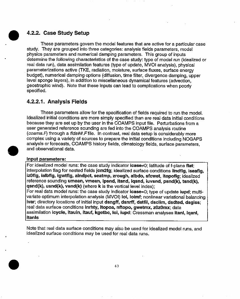
4.2.2. Case Study Setup
These parameters govern the model features that are active for a particular casestudy. They are grouped into three categories: analysis fields parameters, modelphysics parameters and numerical damping parameters. This group of inputsdetermine the following characteristics of the case study: type of model run (idealized orreal data run), data assimilation features (type of update, MVOI analysis), physicalparameterizations active (TKE, radiation, moisture, surface fluxes, surface energybudget), numerical damping options (diffusion, time filter, divergence damping, upperlevel sponge layers), in addition to miscellaneous dynamical features (advection,geostrophic wind). Note that these inputs can lead to complications when poorlyspecified.
4.2.2.1. Analysis Fields
These parameters allow for the specification of fields required to run the model.Idealized initial conditions are more simply specified than are real data initial conditionsbecause they are set up by the user in the COAMPS input file. Perturbations from auser generated reference sounding are fed into the COAMPS analysis routine(coama.F) through a flds##.Ffile. In contrast, real data setup is considerably morecomplex using a variety of sources to prepare the initial conditions including NOGAPSanalysis or forecasts, COAMPS history fields, climatology fields, surface parameters,and observational data.
Input parameters:For idealized model runs: the case study indicator icaseO; latitude of f-plane flat;interpolation flag for nested fields jcm2fg; idealized surface conditions ilndflg, iseaflg,izOflg, ialbflg, igwtflg, alndpct, seatmp, zrough, albdo, sfcwet, itopoflg; idealizedreference sounding umean, vmean, ipsnd, itsnd, iqsnd, iuvsnd, psnd(k), tsnd(k),qsnd(k), usnd(k), vsnd(k) (where k is the vertical level index);For real data model runs: the case study indicator icase=O; type of update iupd; multi-variate optimum interpolation analysis (MVOI) loi, loimf; nonlinear variational balancingivar; directory locations of initial input dsngff, dsnrff, datfil, dsclim, dsdted, dsgiss;real data surface conditions lnrhty, Itopoa, nftopo, gwetmx, zOzOmx; dataassimilation icycle, itauin, itauf, kgetbc, loi, iupd: Cressman analyses Itanl, Iqanl,Itanls
Note that real data surface conditions may also be used for idealized model runs, andidealized surface conditions may be used for real data runs.
43

4.2.2.2. Model Physics
COAMPS contains many inputs that govern various parameterization options forspecifying the surface and boundary layers, moist physics, convection and radiationschemes. Refer to Appendix D for further definitions.
Input parameters:surface layer processes If lux, Isfcen, lies; boundary layer processes Itke, iahsgm,iamxgl, iashsm, shO, smO, lies; moist and convective processes ilsp, Imoist, lice,Icupar, cupd; radiative processes Irad, dtrad, njump, Icool; vertical advection of TKE,rain and snow dxmeso, dzqlim
4.2.2.3. Numerical Damping
To control numerical instability and the growth of unrealistic tendencies, severaldamping features have been added to the COAMPS code.
Input parameters:diffusion and filtering Idiff, dif2nd, dif4th, Ifft; divergence damping Iddamp, divdmp;time filtering robert; upper level sponge layer Iralee, rdtime, nrdamp, Ispong
4.2.2.4. Additional Model Features
These parameters provide options for the advective scheme (e.g. 2nd order, 4 thorder, flux or advective schemes) and allow for adding a large scale pressure gradientvia the geostrophic wind.
Input parameters:advection scheme iadvct; geostrophic wind Ivgeo, ugeo, vgeo
4.2.3. Data Manipulation
Several namelist parameters are used to control the flow of data into and out ofthe COAMPS system. These inputs are categorized into three groups: data input andoutput parameters (used for analysis, restarts and data assimilation purposes), graphicsparameters (used to view model output), and diagnostic parameters (used tonumerically evaluate model results).
Input parameters:
44
directory locations dsngff, dsnrff; times for printing/saving output kprnta, ksavea,ksaves, isavefrq, ifsave; data format type Iwritu; 1 D graphics output dsetl d, ti d,ild(nn), jld(nn), cpar(nn), city(nn); 2D graphics output npfil, xsfil, lwritu; 3D graphics

output tvisl, tvis2, vparl, vpar2, lprvis, prsvis, hgtvis, ksaves, Iwritu; diagnosticoutput laper, lasym, Idgadj, lcuppr, lprnti
Although most of these output times are designated by time intervals, note thatparameter ksaves is an array containing actual times during the forecast that 3Dvolumes of sigma level data are to be saved. Caution is advised when outputting 3Dvolumes over a long forecast period or at many times, especially for more than onemesh since they are quite large (a (65x65x30) grid requires approximately 1 OOMb ofspace).
Having reviewed the more important COAMPS input parameters in this section,and using Appendix B as an example of a COAMPS input file, the user is now able tocreate a COAMPS input file that sets up any type of model run. The final step inperforming a COAMPS simulation is to submit the run job as described in the nextsection.
4.3. Submitting a COAMPS Job
The user is ready to submit a COAMPS job once the following steps have beencompleted:
1. The analysis and forecast codes have been compiled and linked to form theCOAMPS executables (coamps analysis. exe and coampsjorecast. exe.
2. The data has been obtained to specify the initial input fields.3. The COAMPS run script run.coamps has been edited to update the namelist input
parameters (i.e. the namelist input file nfistinput has been modified to suit theparticular process study).
In the example given below, the COAMPS run script template, run.coamps, has beenmodified and renamed run.runsd where runsdis a user-created subdirectory under/run.This script creates a COAMPS namelist input file called nfist.$ddtg.runsd where $ddtgis the a 10 digit date-time group (YYYYMMDDHH) provided to the script file as an inputargument.
Within the /run/runsd subdirectory, submit the run script by typing: "run.runsd$ddtg 3". The first input argument represents the starting date-time group. Thesecond is a run action argument indicating whether the analysis or forecast is to be run.
Table 6: Options for the 2nd run script input argumentARGUMENT ACTION0 no action1 run analysis2 run forecast3 run analysis and forecast
45
When the second input argument is '1' or '3', the run script executes the analysis Wprogram using the following command:
$HOMEfcoamps/bin/coamps-analysis.exe < nhist.$ddtg.runsd > output.a.$ddtg
The user input is redirected into the analysis program from file nfist.$ddtg.runsd andstandard output/error is redirected out to file output.a.$ddtg. Upon completion, thedirectory specified by namelist input dsnrff contains the analysis fields produced by theexecutable. Scan this directory and view the file output.a.$ddtg to ensure that theanalysis completed successfully.
Similarly, when the second input argument is '2' or '3', the run script executes theforecast using the following command:
$HOME/coamps/bin/coampsforecast.exe < nlist.$ddtg.runsd> output.m.$ddtg
User input is redirected into the forecast program from file nlist.$ddtg.runsd andstandard output/error is redirected out to file output.m.$ddtg. Upon successfulcompletion of the COAMPS forecast, user-requested forecast fields reside in thedirectories specified as namelist input dsnrff and dsetl d. These data may be viewedgraphically with a variety of display packages that process 1 D, 2D or 3D model outputthe details of which are covered in a separate document. For a quick analysis of theCOAMPS results at time intervals given by the user input parameter kprnta, the user 0may look at 'quick prints' of horizontal and vertical slice numerical model outputembedded in the standard output/error file outputm.$ddtg. The output to this file alsoindicates whether the job has completed successfully.
A data assimilation update cycle may be submitted by inputting two additionalrun script arguments. The third input argument is a 10 digit ending date-time group(YYYYMMDDHH) and the forth argument is the number of hours between updates(typically 12 hours). To submit a 12 hour data assimilation cycle, the user types:"run.runsd $ddtg 3 $enddtg 12". The command initiates a forecast starting at $ddtgand continuing through $enddtg assimilating data every 12 hours. This type of run isonly appropriate when observations are available every 12 hours throughout the timeperiod since these data are needed to adjust the first guess fields.
46

Appendix A: Sample makefile
This Makefile template is from the /coamps#/mod/Templates directory that is created byrunning the script file get.templates for the SGI machine Rossby.
file .Jvfakf7lh;
I -- . ~ ~ T77~~ 7~T7 ..... A.j j* j~~i i._j,,i, ,i.,;, ~ i ,,* r,.. r 'r'.' ii.' N.; "Fr.rm FT, _ii T.r , ' r ,' .y'r 77ijj~j Fjr j r r,' ,= iij-.r.,' :'-r Hr i
. ~ ~ ~ ~ ~ ~ ~ ~ ~ ~ ~ ~ ~.- .~~~~~~~~~~ j.. irl'l.':;iii" lO htuii 1( 7,oI al ('gtu i ~~lT)s anlak iocx and ~oarnp-].__'otecas.cxe'~ a : c m
~~r---...-,iH..i.-j ~ ~ ~ ~ ~ ~ ~ . ,;iiij jFi-,i~~F,,,, ~ ii---ir~r i- i:~iiiFF r - ,irr,--ri i-i-iiHF-1 F-....-..........- N.7 .N~U1
oilier doip cndomics .7i,--
iwlclude /data wl b' 6/usc rM/coalnps/coanms2.0/conth!.os
include /datarossby6/users/coamnps/coamps2.0/config.user
LBDIR = /datarossby6/users/coamps/lib/2.0MAINANL = /data_rossby6/uscrs/coamps/coamps2.0/src/coamps-analvsis/coamps-analysis.F ;MAINFCST = /data-rossby6/uscrs/coamps/coamps2.0/src/coamps-forecasi/coampsjforecast.F:INCLPROL_MAIN = /dataL rossby6/users/coamps/coainps2.0/prologues/main INCL_.ROLCOAMPS = /datarossby6/uscrs/coamps/coarnps2.0/prologues/coampslibINCL_PROL_0 I= /daiarossby6/users/coamps/coamps2.0/prologues/oilib
LEBS =S. SLIB3I)IR).'coamnpslib~
s:, Li 13DI.)R.'fioc..ib.a 'S(L1 13D)I R)/ili \:.a
S(L.IB t).lR)/c;a.nipsl l.a \ .* $(13BlDR)inl.. bKhqlib.a \S(l..1131)1IR'Wfishlpaklil.a
MAKFILE =Makefile
# OBJS: include the coamps .o files that the user modified
PROGRAMS= coamps analysis.exe
coamps forecast :xe
target : $(PROGRAMS) $(IOBJS) $(L) ': (cotnned .
A-1
e
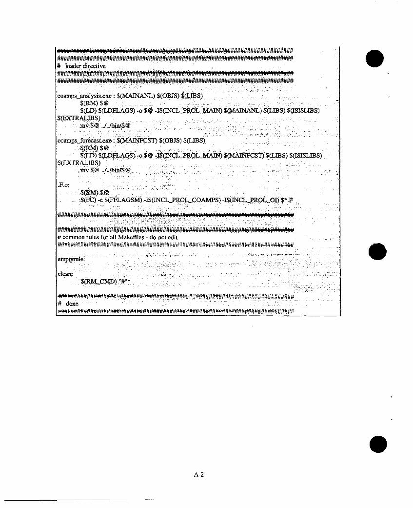
wa~~~~~ ~~ it At0 a 0#w w s# a} A s wa gg~ iwsw rrJ a gif Jt a m g l u v 4 l %F i I l Art; t 1; 4 w 11 w P; f; t Wf iss r~Fgi g a i i F; u s Ig v sp wi ;Fs} Og ;Im;; ut g;l 4
coamnps...anilysis.exe: $(MAINANIL) $(OBJS) $(L~SS(RM) $@$(LD) $(LDFLAG)-o $@-I$(]NCL.PY ~ J)$MIAL $LB)$IL2S
$(EXTRALIBS)
coa epsrjorecasLexe: $(MAJFCST) S(OBJS) $(LIBS),
5(TD)) t,(LDFAGS 7o$@4 C2O..MN)$OVMAWCST).$(LIBS) $(ISISLIBS)s(rExrRALIBS)
-mv $@J../j$
-.Ro:
-,$(FC) -c $(FFLGM I(NLPOOMS -IS NLYPROLOI) $*.F
"""" " " " ""'!:" " "" !"" !':" ".."":''"".""" !s ."..11!1-,. !.1 Z w :;..J 1* "-.J. sl~} .- Zs d .,iS...$ sJ! llfU A.LI
;r C~ )IfliflO I1 r u k ~ f o r iii \la k ~ h I~ % Md n o -F-ditr r
eniptYrule:
= J1: : U i :coapsanlyssxc $(ANA L $(0BJS)~,; $,(L 7, ,. . ; , ..
#done*
(RT*)7 asa .... ,= j-: AH~~i !i- if ;- - .. ...U:- --- ': -- I: -U-: --. -J f : I...............................:$(LD)~~~~~am S(DS4o$ I(C...GL :,. $S F3DS$(X;XIRALIBS)~~~~~~~71 , -1-1-M0 ,,, : ,, 4! -, ,,H7-,
:$,r7 .:7Af- : ,17: U ?.?777.?.1....1!.r...tff : 1:2tf:::: :::v n) s) ~~~~~-O2@$nSLB)$1ILS

Appendix B: Sample COAMPS user input file nlist.input
file nlist.input&gridnl
kka 30'3ma = 65,73, 109,na =:65,, 73, 91,nbdypt = 7,nnest= 3,
&end
&coanm. i
dscLimr='insert-directory path of climatology data',dsdted= 'inisect directoiry pad] oi'km terrain data',dsgiss = 'inscrt. d;reci.orV pilih ol' Goddard Institute of Space Studies data'.dsngff='innrt directory path oi'NOGAPS flat files',dsnrff= 'insert dircctory path of COAMPS flat files',
npfil ='insert name of ocards file: 2D horizontal graphics directives',."xsfl = 'insert name of xcards file: 2D vcrtical graphics directives',
icase = 0,ibdya:= 7,jbdya = 7,-kgetbc= 12,nproj = 2,aInnt = 5.0,phntl = 600,.,phrt = 30.0,riatl = 45.0.riongi = 5.0,iref = 33,jref = 33,ii u: = 21,20Ji 18, 17delk - 81000..,dely = 8ICO''.0.,delta 240'.0,ktaust= o,o o, ktauf - 24-,0,Ot.
24, 0.0
24;,0,0J,.mtaua = 2,alpha-= 1.0,dsigma = 7500.0, 580(.).0, 4200.0, 2500.0, 1000.0.
100(.(. 750.0.70.0. 750.0. 750.0,'750.0, 750.0,. 1 000.0. 1000.0, 1000.0,1000.0O, 800.0. 800.0, 800.0, 600.0,400.0, .300.0, 200.0, 140.0. 90.0,60.0, 40.0, 30.0. 20.0, 20.0, (coninued)
B-1

Idiff-t,dif2nld=dif4Th=Idda ,m~ = tdivd~m, p=Iralee = fTdtime=
U ur~obrt,_ I2wa~y =-f
Lvgeo =f,iadvct= 2,car= 24
itaxin= 12,itauf= 2,icycle= 12,iupd = 0,'loi =f,loim =f
=rhty=f,Iqan1 f,
Itan=f,lpseud f,ivar =0
Icupar t,lcuppr =f,Imoist =lice =t,had =t,njump= 1,icool =jIsfeen =ml =txlinit = t,
lles = f,ltke = t,aliin =alO =shO =smO =ihsgm =iamnxgl =iashsm =
.11
0.IC
0,
0.04,
50.0,
50.0,
)0.2,
A0, I
0$~~~~~~~~~~~~~~~~~~~: 675, ::
L5 ,: i J
4,4,
ilndflg= 1,ialbflg = 1,iz0fig= 1,igwtflg= 1,iseaflg = 1,itopofig = 1,Itopoa= t,
B-2
(continued)
, . .. . - . . I I 1. . I.... . " ..
0

nftopo = 3,
kpmta = 48, 0,0 .ksavea = 144, 0, 0,ifsavc = 2ksaves = 24, 0, 0.Iwritu = LIpmti = f,locard =.f,ldbms = f,Idbmsi = f,Idbmso = f,
&end
&mvoinl
datfil = 'insert directory path of observational data'
&end
B-3

0
9
I
0
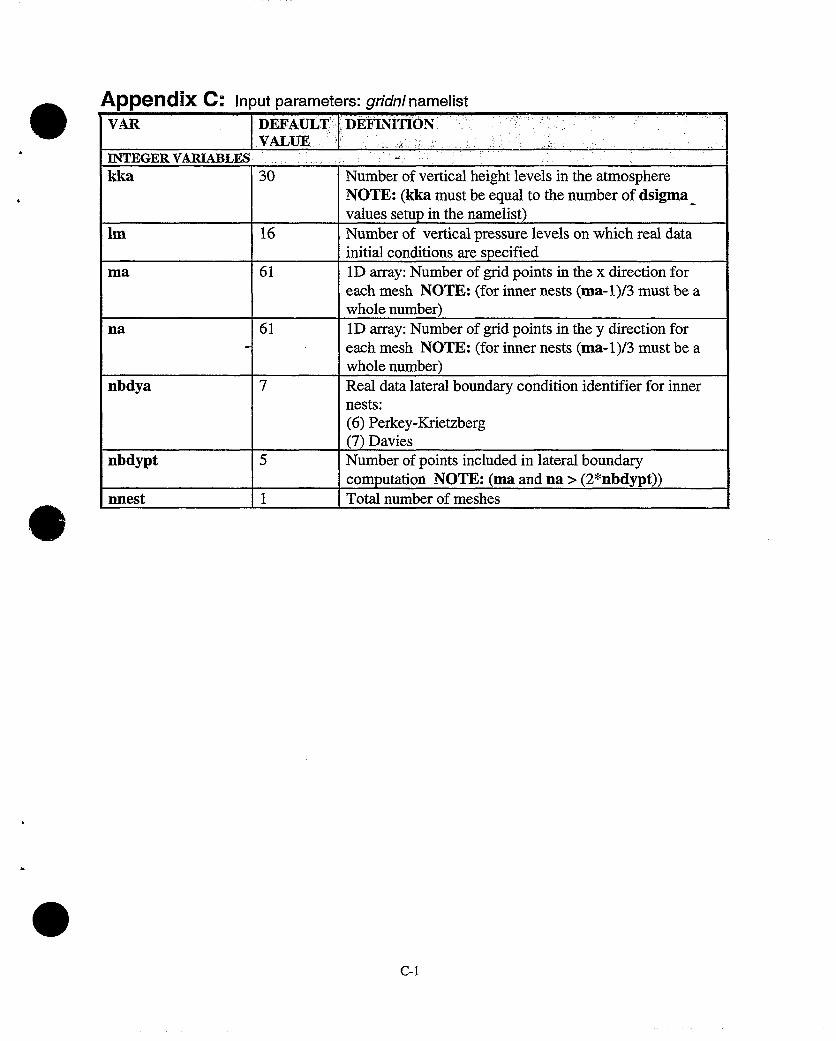
Appendix C: Input parameters: gridni namelistVAR DEFAULT DEF4INIT I O.N-
VALUEINTEGERVARIABLES : ._::_:_____'_'-_'_-_._______________._
kka 30 Number of vertical height levels in the atmosphereNOTE: (kka must be equal to the number of dsigma
___________ values setup in the namelist)IM 16 Number of vertical pressure levels on which real data
initial conditions are specifiedma 61 ID array: Number of grid points in the x direction for
each mesh NOTE: (for inner nests (ma-1)/3 must be awhole number)
na 61 ID array: Number of grid points in the y direction foreach mesh NOTE: (for inner nests (ma-1)/3 must be awhole number)
nbdya 7 Real data lateral boundary condition identifier for innernests:(6) Perkey-Krietzberg(7) Davies
nbdypt 5 Number of points included in lateral boundarycomputation NOTE: (ma and na > (2*nbdypt))
nnest 1 Total number of meshes
C-l

.
0
0
I
0

Appendix D: Input parameters: coamnl namelistAR DEFAULT VALUE DEFINITION
CHARACTERVARIABLES : . _.,_______i__..,________:.::'.:._
city ' Character*32, 2D array: City names associated withgrid point locations (ildjid) for each mesh; used for
.______________________ labeling ID graphics output (getld.F, asavld.F)cpar . Character*4, 2D array: lD graphics variable
identification string for each mesh; used to selectvariables for ID graphics output (getld.F, asavld.F)
dsclim '/home/hodur/masterr/' Character*80: Directory path of climatology data;used to initialize the real data surface parameters(albedo, sst, grdwet, rHand, zsfc, zO) when highresolution data not available (sfcpar.F, soiltp.F)
dsdted '/u/c/hodur/masdted/' Character*96: Directory path of 1 km terrain data;used for horizontal resolution < 20 km and if available(sfcpar.F)
dsgiss '/a/ops/etc/static/met Character*80: Directory path of Goddard Institute/noraps/masgiss/' Space Studies high resolution albedo and zO data
(sfcpar.F)dsetng l Character*24: ISIS directory path of NOGAPS data
input/output; used for location of boundary conditionsand/or cold start initial conditions when Idbms=.true.(gethty.F, getng.F, getsst.F, inhesc.F, inngsc.F,innguv.F)
dsetg l Character*24, ID array: ISIS directory path ofCOAMPS data input/output for each mesh; used forlocation of COAMPS files when ldbms=.true.(gethty.F, getng.F, getsst.F, inhesc.F, inngsc.F,innguv.F)
dsetld './' Character*80: Directory path for ID graphics output(get]d.F, asavld.F)
dsngff l Character*80: Directory path of NOGAPS flat files;used for location of boundary conditions and/or coldstart initial conditions when Idbms=.false. (gethty.F,getng.F, getsst.F, inn gsc.F, innguv.F)
dsnrff . Character*80: Directory path of COAMPS flat files;used for location of COAMPS input/output needed forincremental update, model restart, and 2D and 3Dgraphics output when Idbms=.false. (coamm.F, io*.F)
gnamg l l Character*32, ID array: ISIS geometry name for eachmesh; used by ISIS when Idbms and Idbmsi=.true.
mdltg l Character*32, ID array: ISIS model type for eachmesh; used by ISIS when Idbms and Idbmsi=.true.
npfil 'ocards' Character*80: name of file containing 2D horizontal
D-1

level plotting information (fields, plot type, level, time,mesh number, etc.)
xsfil 'xcards' Character*80: name of file containing 2D cross-sectional plotting information (fields, plot type, levels,time, mesh number, etc.)
vparl l Character*4, 2D array: 3D graphics variableidentification string set 1 for each mesh; used to selectVisual output (visout.F)
vpar2 l Character*4, 2D arrays: 3D graphics variableidentification string set 2 for each mesh; used to selectVisual output (visout.F)
REAL VARIABLES
albdo 0. 2 Idealized value of surface refractivity; used to specifythe albedo when ialbflg= o (userijsfce.F) NOTE:(0.0 = low refractivity, 1.0 = high refractivity)
alndpct 1.0 Idealized land/water indicator; used to specify whethera point is a land or water point when ilndflg = o(usersfc.F) NOTE: (0.0 = water, 1.0 = land)
alnin 0.02 m Minimum mixing length factor (afore.F)alnnt 240.0 0 Longitude aligned north-south; used for rotating a
lambert conformal/polar stereographic projection(grid.F) NOTES: (increases eastward from 0° to 360°beginning at Greenwich, England) (longitudes outsidethe model domain may be used to rotate the grid)
alpha 0.4 Averaging coefficient for semi-implicit timedifferencing (alhs.F, alhsin.F).
alO 100.0 m Mixing length constant/limiting value (coamnLF)cbar 100.0 m/s Speed of sound cbar=c-,cRT7,/ cV (alhs.F, alhsin.F,
asetim,]) NOTES: (if cbar<O, value computed incoamm.F) (because of numerical techniques,cbar 2 2*1VI)
climrh .01,.0I,.01,.02,.02,.10,.15 ID array: Climatological values of relative humidity at,.20,.25,.30,.40,.50,.60,.70 user specified pressure (pr) levels (geing.F).,.70,.70,84*.70
estar 300.0 rn/s Speed of gravity waves cstar = (ZT!7r)V(g/o9)d0v,/dz
where Zt the is domain top; used for radiative lateralboundaries (ibdya=jbdya= 4 or 5) (bwind.F)
cupdx 10000.0 m Minimum horizontal resolution for Kain-Fritschconvective parameterization scheme (amodel.F)
delta 2.0 s Large, coarse mesh time step; used for integration ofslow modes NOTE: (cfl condition: delta < dsigma/w& delta < 0.7*delx/(2*IVI)) (inner nest time steps
D-2
.VAR I� DEFAULT VALUE DEFEINITION

VDEAULT VALUEcomputed internally)
delx 40000.0 m (specify in Coarse mesh grid spacing in the x-direction; used fordegrees of longitude when computing horizontal spatial derivatives NOTE:nproj=5) (inner nest spacing computed internally)
dely 40000.0 m (specify in Coarse mesh grid spacing in the y-direction; used fordegrees of latitude when computing horizontal spatial derivatives NOTE:nproj=5) (inner nest spacing computed internally)
dif2nd 0.01 2nd order dimensionless diffusion coefficientdif2nd=Kd2At/Ax2 • 1/8 for stability; used to controlsmall scale numerical noise (asetup.F)
dif4th -0.0025 4th order dimensionless diffusion coefficientdif4th=KdtAt/Ax4 > -1/32 for stability; used to controlsmall scale numerical noise (asetup.F) NOTE: (ifnon- negative, 2nd order diffusion is used)
divdmp 10.0 Dimensionless divergence damping coefficientdivdmp=Kd1 A/Ax2 < 1/2 for stability; used to controlamplification of the acoustic mode (alhs.F) NOTE:(smaller values produce greater damping)
dsigma 500.0 m ID array: Vertical grid spacing in the atmosphere; usedto compute vertical spatial derivatives NOTE: (nonuniform vertical spacing is permitted)
dtrad 3600.0 s Radiation time interval; used to determine frequency ofradiation computations (coamm.F)
dxmeso 9000.0 m Upper limit of horizontal resolution below which thevertical advection of tke, raindrops and snow areincluded in prognostic equations (afore.F, aforqx.F)
dzqlim 500.0,250.0,100.0,100.0, Upper limit of height, for each mesh, below which100.0,100.,100 m vertical spacing for vertical advection of rain and snow
is computed (dzqrs.F)flat 0.0 0 Latitude; Used for Cartesian grids (nproj=4) to
compute the Coriolis parameter (grid.F)gwetmx 1.0 Maximum ground wetness (sfcpar.f)hgtsnd 999.0 m ID array: Heights above surface of idealized sounding
data (refsnd.F) NOTE: (computed internally)hgtvis 10., 50., 100., 200. ID array: Heights above the surface that 3D graphics
300., 400., 500., 750. data are interpolated to; used for Visual output when1000.,1250., 1500., 2000. lprvis=.false. (visout.F)2500.,3000., 3500., 4000.4500.,5000., 6000., 7000.8000.,9000.,10000.,12000.
,15000.,75*0.0 mphntl 30.00 Latitude where map projection intersects the earth and
I______ Imap factor is 1.0; used to setup map projection (grid.F)
D-3
VAR DEFINITION
0
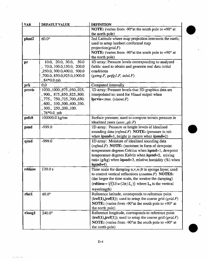
DEFAULT VALUE
t
DEFINITIONNOTE: (varies from -900at the south pole to +900 atthe north pole)
phnt2 60.00 2nd Latitude where map projection intersects the earth;used to setup lambert conformal mapprojection(grid.F)NOTE: (varies from -90'at the south pole to +900 atthe north pole)
pr 10.0, 20.0, 30.0, 50.0 lD array: Pressure levels corresponding to analyzed70.0, 100.0,150.0, 200.0 fields: used to obtain and generate real data initial
,250.0, 300.0,400.0, 500.0 conditions,700.0, 850.0,925.0,1000.0 (getng.F, gelfgl.F, inlvl.F)84*0.0 mb
prk 0.0 Computed internallyprsvis 1030.,1000.,975.,950.,925. iD array: Pressure levels that 3D graphics data are
. 900., 875.,850.,825.,800. interpolated to; used for Visual output when,775., 750.,725.,700.,650. Iprvis=.true. (visout.F), 600., 550.,500.,400.,350., 300., 250.,200.,100., 76*0.0 mb
psfcO 100000.0 kg/ms Surface pressure; used to compute terrain pressure inidealized cases (user sfc.F)
psnd -999.0 iD array: Pressure or height levels of idealizedsounding data (refsnd.F) NOTE: (pressure in mbwhen ipsnd= 1, height in meters when ipsnd=2)
qsnd -999.0 1D array: Moisture of idealized sounding data(refsnd.F) NOTE: (moisture in form of dewpointtemperature degrees Celcius when iqsnd=1, dewpointtemperature degrees Kelvin when iqsnd=2, mixingratio (g/kg) when iqsnd=3, relative humidity (%) when
.______ ______iqsnd=4)
rdtime 120.0 s Time scale for damping u,v,w,O in sponge layer; usedto control vertical reflections (coamm.F) NOTES:(the larger the time scale, the weaker the damping)(rdtime 1/(3.5 w (27r/L, )) where L, is the verticalwavelength)
rlatl 40.00 Reference latitude, corresponds to reference point(iref(1),jref(l)); used to setup the coarse grid (grid.F)NOTE: (varies from -900at the south pole to +900 atthe north pole)
rlongl 240.00 Reference longitude, corresponds to reference point(iref(1),jref(l)); used to setup the coarse grid (grid.f)NOTE: (varies from -900at the south pole to +900 at
Ithe north pole)
I
D-4
VAR
1�
IS
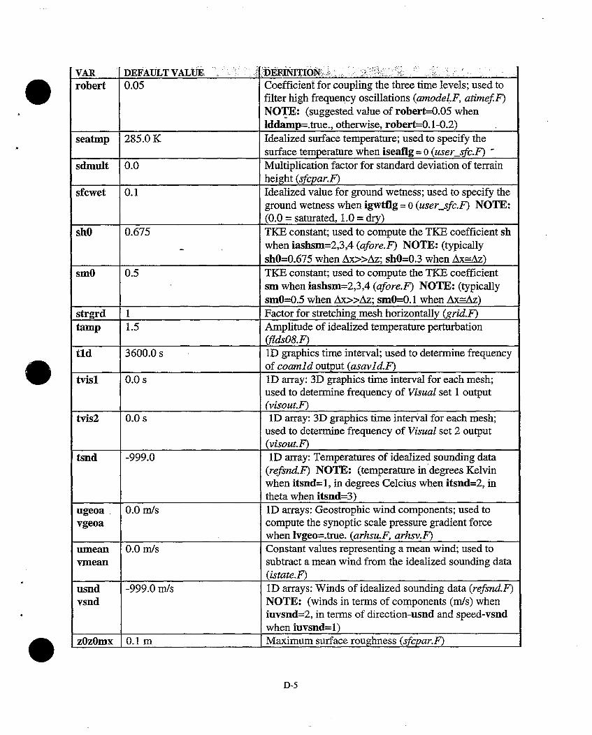
VAR DEFAULT VALUE ' ' , DEFI-FITION,,, ' , -' ; i - !
robert 0.05 Coefficient for coupling the three time levels; used tofilter high frequency oscillations (amodel.F, atimef.F)NOTE: (suggested value of robert=0.05 whenIddamp=.true., otherwise, robert=0.1-0.2)
seatmp 285.0 K Idealized surface temperature; used to specify thesurface temperature when iseafig= 0 (user sfc.F)
sdmult 0.0 Multiplication factor for standard deviation of terrainheight (sfcpar.F)
sfcwet 0.1 Idealized value for ground wetness; used to specify theground wetness when igwtflg = o (users. sfc.F) NOTE:(0.0 = saturated, 1.0 = dry)
shO 0.675 TKE constant; used to compute the TKE coefficient shwhen iashsm=2,3,4 (afore.F) NOTE: (typicallyshO=0.675 when Ax>>Az; shO=0.3 when Ax-Az)
smO 0.5 TKE constant; used to compute the TKE coefficientsm when iashsm=2,3,4 (afore.F) NOTE: (typicallysmO=0.5 when Ax>>Az; smO=O. 1 when Ax=Az)
strgrd 1 Factor for stretching mesh horizontally (grid.F)tamp 1.5 Amplitude of idealized temperature perturbation
(fldsO8.F)tld 3600.0 s ID graphics time interval; used to determine frequency
of coamld output (asavld.F)tvisl 0.0 s iD array: 3D graphics time interval for each mesh;
used to determine frequency of Visual set 1 output(visout.F)
tvis2 0.0 s ID array: 3D graphics time interval for each mesh;used to determine frequency of Visual set 2 output(visout.,F)
tsnd -999.0 iD array: Temperatures of idealized sounding data(refsnd.F) NOTE: (temperature in degrees Kelvinwhen itsnd= 1, in degrees Celcius when itsnd=2, intheta when itsnd=3)
ugeoa. 0.0 m/s ID arrays: Geostrophic wind components; used tovgeoa compute the synoptic scale pressure gradient force
when lvgeo=.true. (arhsu.F, arhsv.F)umean 0.0 m/s Constant values representing a mean wind; used tovmean subtract a mean wind from the idealized sounding data
(istate.F)usnd -999.0 mI/s D arrays: Winds of idealized sounding data (refsnd.F)vsnd NOTE: (winds in terms of components (m/s) when
iuvsnd=2, in terms of direction-usnd and speed-vsndwhen iuvsnd=l)
zOzOmx 0.1 m Maximum surface roughness (sfcpar.F)
D-5
1I

zrough 0.01 m Idealized value for surface roughness; used to specifythe surface roughness when izOflg = 0 (user..sfc.F)NOTE: (0.0 = smooth, 1.0 = rough)
INTEGER VARLABLES
iadvct 1 Advection type identifier (arhs*.F, afor*.F, advsc.F):(1) 4th order advective(2) 2nd order advective(3) 2nd order advective with 2nd order upstream for 0(4) spectral(5) 2nd order flux(6) mixed: 2nd order advective and flux
ialbflg I Indicator for use of idealized albedo data for each mesh(user..sfc.F) (NOTE: albedo given by idealized value(albdo) when ialbflg=O, otherwise uses database)
iahsgm 1 Horizontal subgrid scale mixing identifier:(arhs*.F, afor*.F, lmix*.F)(1) eddy mixing coefficient based upon deformationfield (use when Ax>>Az)(2) eddy mixing coefficient based upon TKEprediction (use when Ax-Az)
iamxgl 1 Mixing length identifier: options for the mixinglengths all, a12, aid are given in Table D-1 below(afore.F,coamm.F)
iashsm 1 TKE coefficients sm and sh identifier; used to defineeddy mixing coefficients (afore.F):(1) Ri dependent (Mellor & Yamada, 74)(2) sm=smO, sh=shO(3) sm=smO, sh=(1.0+2.0 al2/all)*smO(4) sm=smO, sh=2.13*smO(5) Ri dependent (Mellor & Yamada, 82)
ibdya I x-direction boundary condition identifier (abdy*.F):idealized(1) fixed(2) extrapolated(3) periodic(4) radiation(5) radiation and extrapolationreal data(6) Perkey-Krietzberg(7) Davies
icase 1 Case number identifier; used to indicate real oridealized data (coama.F, flds##.F):(0) real data(##) value corresponds to the number inflds##.F
D-6
0
IVAR, I DEFAULT VALUE I DEFINMON

I DEFAULT VALUEfilename, a file where perturbations of the mean stateare specified
icycle 0 hr. Frequency of a data assimilation cycle; used toread/write input/output fields (coama.F, coamm.F)
idgadj 2 x-grid point; used for printout of microphysicaldiagnostics (adjtq.F)
ifsave 1 Indicator for saving sigma level data (coamm.F):(1) at specific times given by ksaves(2) at time intervals given by isavfrq
igwtflg 1 Indicator for use of idealized ground wetness for eachmesh (usertjsfc.F) (NOTE: ground wetness given byidealized value (sfcwet) when igwtflg=O, otherwiseuses database)
ii 21 ID array: Parent meshes x-grid point corresponding toleft boundary of next inner nest; used to setup innernests (coama.F)
ilndflg 1 Indicator for use of idealized land/sea grid point foreach mesh (user..sfc.F) (NOTE: land/sea point givenby idealized value (alndpct) when ilndflg=O,otherwise uses database)
iloi 0 MVOI volume type identifier (coama.F):(0) ivol, jvol = number of MVOI volumes(1) ivol, jvol = distance in kilometers of an MVOIvolume
ilsp 1 Indicator for use of explicit moist physics for eachmesh (amodel.F) NOTE: (explicit moist physicswhen ilsp=l, large scale precip param when ilsp=2)
ipsnd 1 Indicator of units of idealized pressure data (refsnd.F)NOTE: (pressure in mb when ipsnd=1, height inmeters when ipsnd=2),
iqsnd 1 Indicator of units of idealized moisture data (refsnd.F)NOTE: (moisture in form of dewpoint temperature'degrees Celcius when iqsnd=1, dewpoint temperaturedegrees Kelvin when iqsnd=2, mixing ratio (g/kg)when iqsnd=3, relative humidity (%) when iqsnd=4)
iref 55 ID array: x-grid point on each mesh at referencelatitude rlatl; used to setup the model domains(grid.F) NOTE: (iref(l) can be larger than ma(l)when alnnt and rlongl fall outside the model domain -- for rotated grids) (iref for inner nests computedinternally)
isavefrq -1,0,0 hr,min,sec Times for saving sigma level data; used to graphicallyview COAMPS forecast fields (coamm.F) NOTE:
D-7
1,VAR
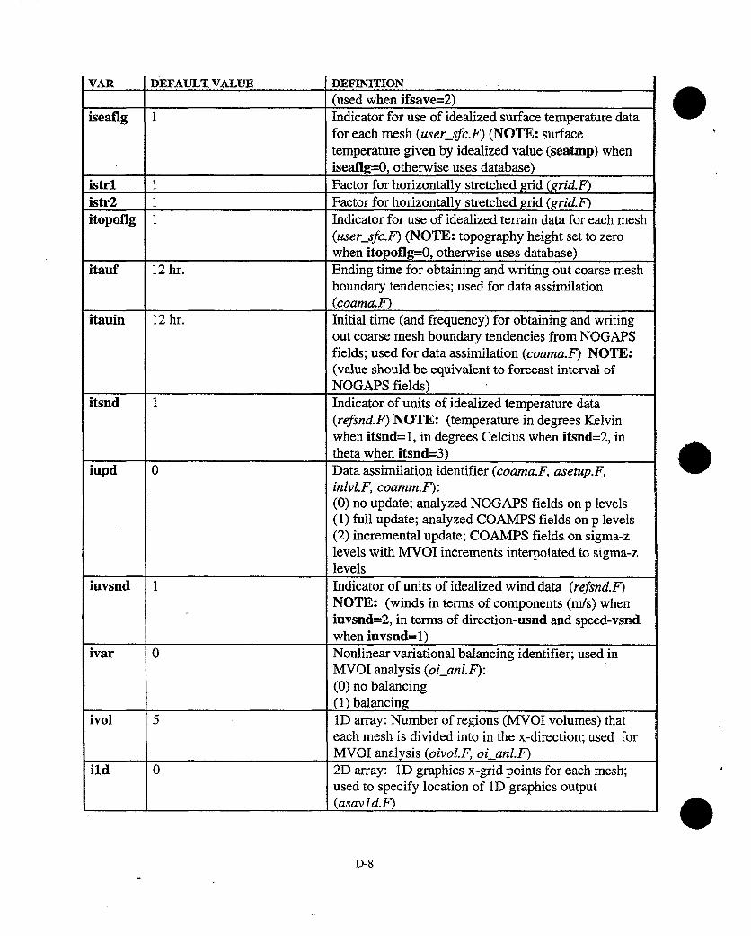
DEFAULT VALUE DEFINITION(used when ifsave=2)
iseaflg 1 Indicator for use of idealized surface temperature datafor each mesh (userj --sfc.F) (NOTE: surfacetemperature given by idealized value (seatmp) wheniseaflg=0, otherwise uses database)
istri 1 Factor for horizontally stretched grid (gtid.F)istr2 1 Factor for horizontally stretched grid (grid.F)itopoflg 1 Indicator for use of idealized terrain data for each mesh
(user..--sfc.F) (NOTE: topography height set to zerowhen itopoflg=O, otherwise uses database)
itauf 12 hr. Ending time for obtaining and writing out coarse meshboundary tendencies; used for data assimilation(coama.F)
itauin 12 hr. Initial time (and frequency) for obtaining and writingout coarse mesh boundary tendencies from NOGAPSfields; used for data assimilation (coama.F) NOTE:(value should be equivalent to forecast interval ofNOGAPS fields)
itsnd 1 Indicator of units of idealized temperature data(refsnd.F) NOTE: (temperature in degrees Kelvinwhen itsnd= 1, in degrees Celcius when itsnd=2, intheta when itsnd=3)
iupd 0 Data assimilation identifier (coama.F, asetup.F,inlvl.F, coamm.F):(0) no update; analyzed NOGAPS fields on p levels(1) full update; analyzed COAMPS fields on p levels(2) incremental update; COAMPS fields on sigma-zlevels with MVOI increments interpolated to sigma-zlevels
iuvsnd 1 Indicator of units of idealized wind data (refsnd.F)NOTE: (winds in terms of components (m/s) wheniuvsnd=2, in terms of direction-usnd and speed-vsndwhen iuvsnd=1)
ivar 0 Nonlinear variational balancing identifier; used inMVOI analysis (oi.anl.F):(0) no balancing(1) balancing
ivol 5 1D array: Number of regions (MVOI volumes) thateach mesh is divided into in the x-direction; used forMVOI analysis (oivol.F, oi anl.F)
ild 0 2D array: ID graphics x-grid points for each mesh;used to specify location of ID graphics output(asavld.F)
D-8
VAR
I
0
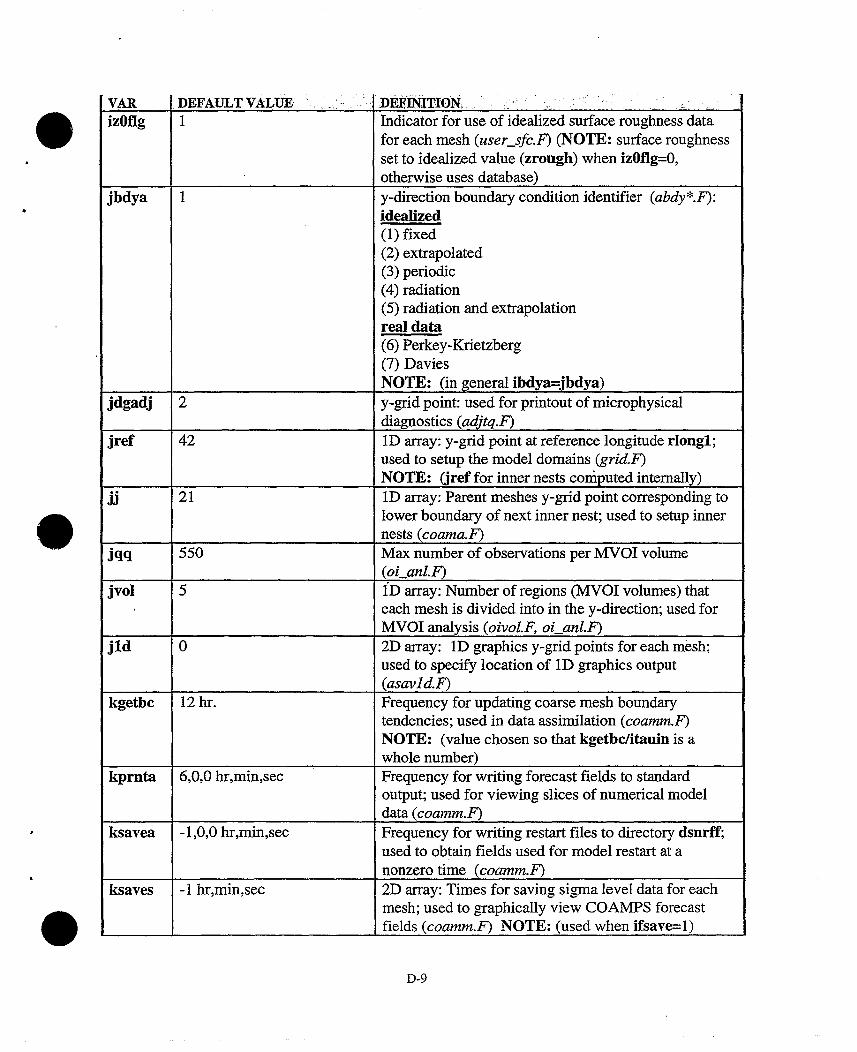
izOflg 1 Indicator for use of idealized surface roughness datafor each mesh (user..ssfc.F) (NOTE: surface roughnessset to idealized value (zrough) when izOflg=O,
._______ otherwise uses database)jbdya 1 y-direction boundary condition identifier (abdy*.F):
idealized(1) fixed(2) extrapolated(3) periodic(4) radiation(5) radiation and extrapolationreal data(6) Perkey-Krietzberg(7) DaviesNOTE: (in general ibdya=jbdya)
jdgadj 2 y-grid point: used for printout of microphysicaldiagnostics (adjtq.F)
jref 42 ID array: y-grid point at reference longitude rlongl;used to setup the model domains (grid.F)NOTE: (jref for inner nests computed internally)
JJ 21 ID array: Parent meshes y-grid point corresponding tolower boundary of next inner nest; used to setup innernests (coama.F)
jqq 550 Max number of observations per MVOI volume(oi anl.F)
jvol 5 iD array: Number of regions (MVOI volumes) thateach mesh is divided into in the y-direction; used forMVOI analysis (oivol.F, oianl.F)
jid 0 2D array: ID graphics y-grid points for each mesh;used to specify location of ID graphics output(asavld.F)
kgetbc 12 hr. Frequency for updating coarse mesh boundarytendencies; used in data assimilation (coamm.F)NOTE: (value chosen so that kgetbc/itauin is awhole number)
kprnta 6,0,0 hr,min,sec Frequency for writing forecast fields to standardoutput; used for viewing slices of numerical modeldata (coamm.F)
ksavea -1,0,0 hr,min,sec Frequency for writing restart files to directory dsnrff;used to obtain fields used for model restart at anonzero time (coamm.F)
ksaves -1 hr,min,sec 2D array: Times for saving sigma level data for eachmesh; used to graphically view COAMPS forecastfields (coamm.F) NOTE: (used when ifsave=l)
D-9
I'D004TIONVAR DEFAULT VALUE

VAR DEFAULT VALUE DEFINMONktauf 12,0,0 hr,minsec 2D array: Ending time of forecast for each mesh
(coamm.F)ktaust 0,0,0 hr,min,sec Beginning time of forecast (coamm.f) NOTE: (ktaust
usually equal to zero except for a model restart - seeksavea to save fields for a model restart)
mtaua 5 Number of small coarse mesh time steps per (delta)large time steps; used for integration of fast modes(alhs.F) NOTE: (cfl condition: deltaua < dsigma/w& deltaua < 0.7*deLx/(cbar+IVI) ) (inner nest timesteps computed internally) (because of numericaltechniques used, mtaua typically set to 2)
nftopo 3 Number of passes through 25-point filter; used tosmooth terrain field (sfcpar.F)
nfpass 3 Number of passes through 9- or 25-point filter; used tosmooth output and analysis fields (fllt9.F, filt25.F)
njump 3 njump-l is number of x- and y-grid points skipped inradiation computations (radiat.F)
noisub 12 Number of processors; for MVOI multitasking(ci anl.F)
nproj 2 Map projection identifier; used to setup the horizontaldomain (grid.F):(1) mercator(2) lambert conformal(3) polar stereographic(4) Cartesian coordinates
_________ ~~~~~~~(5) sphericalnrdamp 8 Number of upper model levels that are in the sponge
layer; used to damp vertical reflections (coamm.F)NOTE: (8 or more layers recommended)
LOGICAL VARIABLESlaper false. Check for aperiodicity at boundaries; used as a check
for idealized cases with periodic boundary conditions(ibdya=jbdya=3) (asyml.F, asym2.F):true - check periodicityfalse - do not do above
lasym false. Check for asymmetry in fields; used as a check foridealized cases with symmetric initial conditions andforcing (amodel.F):true - check for asymmetryfalse - do not do above
Icool .false. Simple radiational cooling (aforth.F):true - cool 2° per day below 10 kmfalse - do not do above
D-10
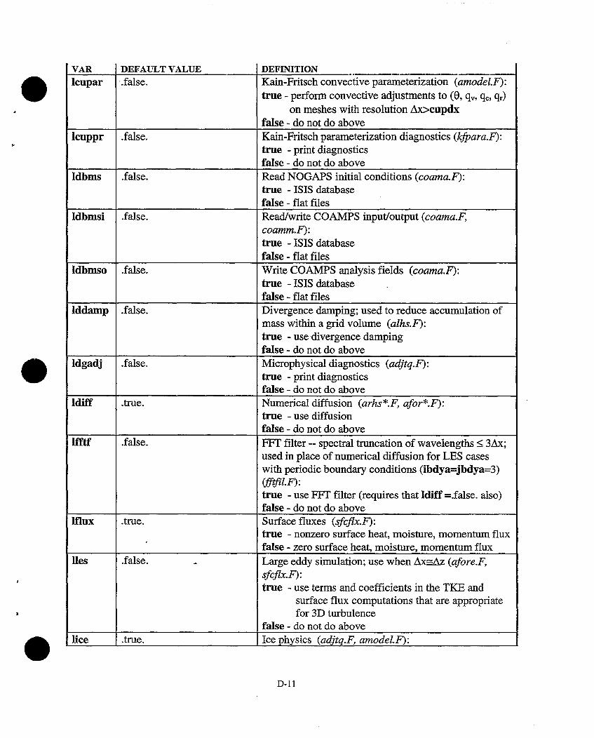
lcupar .false. Kain-Fritsch convective parameterization (amodel.F):true - perform convective adjustments to (0, qv, qc, qr)
on meshes with resolution Ax>cupdxfalse - do not do above
lcuppr .false. Kain-Fritsch parameterization diagnostics (kfpara.F):true - print diagnosticsfalse - do not do above
ldbms .false. Read NOGAPS initial conditions (coama.F):true - ISIS databasefalse - flat files
ldbmsi .false. Read/write COAMPS input/output (coama.F,coamm.F):true - ISIS databasefalse - flat files
ldbmso .false. Write COAMPS analysis fields (coama.F):true - ISIS databasefalse - flat files
Iddamp .false. Divergence damping; used to reduce accumulation ofmass within a grid volume (alhs.F):true - use divergence damping
_______ false - do not do above
Idgadj .false. Microphysical diagnostics (adjtq.F):true - print diagnosticsfalse - do not do above
Idiff .true. Numerical diffusion (arhs*.F, afor*.F):true - use diffusionfalse - do not do above
Ifftf .false. FFI' filter -- spectral truncation of wavelengths < 3Ax;used in place of numerical diffusion for LES caseswith periodic boundary conditions (ibdya=jbdya=3)(fi.iF):true - use FFI' filter (requires that Idiff =.false. also)false - do not do above
Iflux .true. Surface fluxes (sfcflx.F):true - nonzero surface heat, moisture, momentum flux
._______ false - zero surface heat, moisture, momentum fluxlles .false. Large eddy simulation; use when Ax=A7z (afore.F,
sfcflx.F):true - use terms and coefficients in the TKE and
surface flux computations that are appropriatefor 3D turbulence
false - do not do abovelice .true. Ice physics (adjtq.F, amodel.F):
D-11
0
VAR DEFAULT V.AkLUE DEFI:ITION

DEFAULT VALUEtrue - temporal variations and adjustments computed
for frozen moisture variables (qi, qs) (requiresthat Imoist=.true. also)
false - set frozen moisture variables to zerolinit false. Initialize certain variables (ainit.F):
Real datatrue - eliminate net inflow/outflow, compute vertical
velocityfalse - do not do aboveIdealized data (based upon value of icase)true - initialize pressure, or potential temperature, or
add perturbations to horizontal windsfalse - do not do above
Imoist true. Moist physics (adjtq.F, amodel.F):true - temporal variations and adjustments computed
for liquid moisture variables (q,, q.) and frozenmoisture variables (qi, qs) when lice=.true. also)
false - set liquid and frozen moisture variables to zeroInrhty .true. Initialization of surface fields (gethty.F, nethty.F):
true - use COAMPS history fields if availablefalse - use other source: NOGAPS, climatology fields
locard .false. Read in 2D horizontal level plotting information(coama.F, coamm.F):true - ISIS operational formatfalse - do not do above
loi .false. Multivariate optimum interpolation (MVOI) analysis(oLanl.F, anlfld.F):true - perform MVOIfalse - do not do above
loimf false. Inner nest MVOI analysis (oiLanl.F, anlfld.F):true - perform MVOI on inner nest fieldsfalse - interpolate coarse mesh increments to inner
nest fieldslprint false. Surface parameter diagnostics (sfcpar.F):
true - print diagnosticsfalse - do not do above
lprvis .false. Visual data vertical interpolation (visout.FJ:true - pressure levels given by the prsvis arrayfalse - height levels (above surface) given by the
hgtvis arrayIqanl .false. Moisture analysis (anlfld.F, oi.anl.F):
true - perform analysis of initial moisture field._______ _false - do not do above
D- 12
IVAR DEFE14MON

Irad .false. Long and short wave atmospheric radiation schemebased on Harshvardhan (coamm.F, amodel.F):true - radiative adjustments to 0 computed when
integration loop coincides with a dtrad timeinterval
false - do not do aboveIralee .false. Raleigh damping layer (coamm.F):
true - damp (u,v,w,0) to mean state in the topnrdamp levels
false - do not do aboveIsfcen .false. Surface energy budget (sfcenr.F):
true - temporal changes in ground temperature andwetness based upon surface fluxes and radiation
false - no temporal changes in ground temperature orwetness
Ispong .false. Sponge layer (coamm.F):true - damp (u,v,w,O) to smoothed values in the top
nrdamp levelsfalse - do not do above
Itanl .false. Temperature analysis (anlfld.F, oiLanl.F):true - perform analysis of initial temperature fieldfalse - do not do above
ltanls .false. Surface temperature analysis (anlfld.F, oi anl.F):true - perform analysis of initial surface temperature
fieldfalse - do not do above
Itke .true. Subgrid scale mixing (afore.F):true - temporal variations in TKE computedfalse - no temporal variations in TKE
Itopoa .true. Topography (coama.F, insfc.F):true - terrain field given by user or by data basefalse -terrain field set to zero
Ivarad .false. Hydrostatic variational adjustment (stdp2z.F,incrup.F):true - adjust pressure and potential temperature
perturbationsfalse - do not do above
lvgeo .false. Geostrophic winds (arhsu.F, arhsv.F):true - include large scale pressure gradient force
computed from ugeo and vgeo arraysfalse - do not do above
D-13
MVAR DEFAULT VALUE:

lvpert .false. Perturbation added to v-component (ainit.F):true - add perturbationsfalse - do not do above
lwritu .false. Formatting of model input/output data:true - unformatted (32-bit IEEE)false - formatted (Se 13.6)
0
D-14
VAR DEFAULT VALUE DEFINMION

Table D- 1: Namelist input options for the TKE mixing length parameter iamxgl. Column one contains thevariables and arrays in the TKE subroutine afore.F that are controlled by specifying values (1)-(5)for iamxffl. The alO is a user defined input and alOO depends on the zero and first moments of TKE.
a12= .76 (t same a12 as (1) same a12 as (1) fna(blht, stab, TKE) . alOOe zK(diagnostically - (stable) (alOO + vc)
computed amixing length) all - (unstable)
al-= alO * zK (AxAyAz)"3 alO&Az all not used all not used(used in a12; (alO + ZK)constant wrt
time)ald= a12 same ald as (1) same ald as (1) fnb(blht, stab, TKE) al2
(used in the TKEdissipation term)
coef= 019+0.74 a12 same coef as (1) same coef as 0.125 0.170
(used in the TKE all (1)dissipation term)
reference Mellor&Yamada Klemp & --- TheIry& Lacarrere Mellor &1974 Wilhelmson 1983 Yamada 1982
1978

01
0
I
0

Appendix E: Three sample map projections, input parameters, and model domains
(a) (b)
-SCALE0 _
U -Cr z- :0 , o 40- 5O-LATITUDE
60- 70- 80- 90*
Figure E-1: Schematic representation of (a) a mercator map projection with standardlatitude at 200N (Haltiner and Williams, 1980), and (b) the corresponding graphshowing variations in map scale factor with latitude (Saucier, 1955).
Table E-1: Namelist input parameters and values for the mercatormap projection shown in Figure E-2.
Namelist Parameters Definition and Usealnnt = ----- not useddelx = 120000.0, coarse mesh (1) grid spacing in the x-directiondely = 120000.0, coarse mesh (1) grid spacing in the y-directioniref(l) = 31, coarse mesh (1) x-grid point corresponding to the reference latitudeii(2) = 15, coarse mesh (1) x-grid point corresponding to left boundary of inner nest (2)ii(3) = , not usedjref(1) = 28, coarse mesh (1) y-grid point corresponding to the reference longitudejj(2) = 15, coarse mesh (1) y-grid point corresponding to left boundary of inner nest (2)jj(3) = not usedma(1) = 61, coarse mesh (1) x-grid pointsma(2) = 91, inner nest (2) x-grid pointsma(3) = --- , inner nest (3) x-grid pointsna(l) = 61, coarse mesh (1) y-grid pointsna(2) = 55, inner nest (2) y-grid pointsna(3) = --- , inner nest (3) y-grid pointsnnest = 2, model domainsnproj = 1, mecator map projectionphntl = 30, latitude where map projection intersects the earth (i.e. map factor=1)phnt2 = ----- not usedrlatl 10.0, reference latituderlongl = 130.0, reference longitude
E-l
1.0 0- 3 0-

-N0 0
- 0
o ~\ toC C
-b 0C II
C-4
11-1
if
:�:4
evil,
IIF,11
bI
b
0 *t*vs\- I.
. . . . . .
J. 0 \...... .i... ,.z,._ ,/.. ........................:..... .:.:
::I::::: .... I;..- ........ ...- -.-~~. . ....... _ ,' -y--. ............................. .. i; --* ---I
~~~~~~~~~~~~~~~~~~.,.... m ,::: :::\:: ::::gs -----:L
.:..':.'.'. ~ ~ ~ ~ ~ .. .. .--- ls ....* A W )-- X '--- ~-~
~~~~~~~~~~~~~. . . . . . ..:!s--*. -O-t!
0)
S
CD
Ii
~0
o .
ID f
a.) C;o Ln
cd cnsa.)
0
* -iD C Q
X u
5CO ,
l l- a.' ? o)
a a.)
oC..) s a
a.E s
.)£22 s
x )
e 3=a o
-0
iOn
i-.r-
on
0
b
b
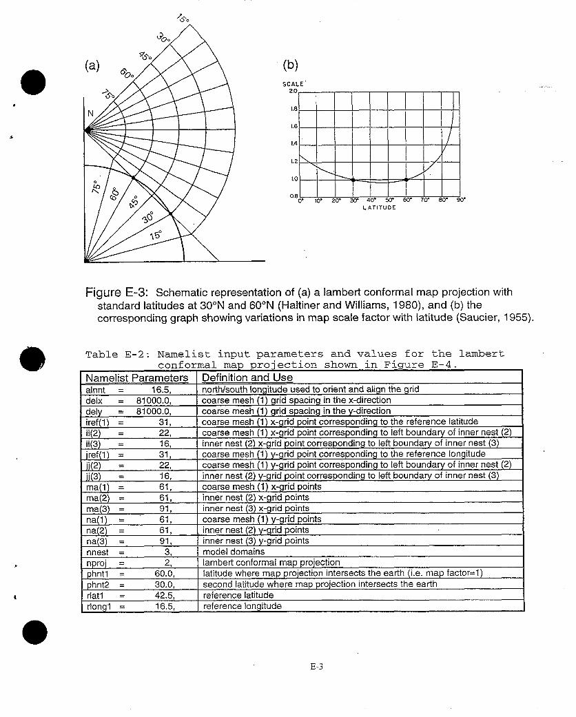
I (b)
SCALE
LATITUDE
Figure E-3: Schematic representation of (a) a lambert conformal map projection withstandard latitudes at 300N and 600N (Haltiner and Williams, 1980), and (b) thecorresponding graph showing variations in map scale factor with latitude (Saucier, 1955).
Table E-2: Namelist input parameters and values for the lambertconformal map projection shown in Figure E-4.
Namelist Parameters Definition and Usealnnt = 16.5, north/south longitude used to orient and align the griddelx = 81000.0, coarse mesh (1) grid spacing in the x-directiondely = 81000.0, coarse mesh (1) grid spacing in the y-directioniref(l) = 31, coarse mesh (1) x-grid point corresponding to the reference latitudeii(2) = 22, coarse mesh (1) x-grid point corresponding to left boundary of inner nest (2)ii(3) = 16, inner nest (2) x-grid point corresponding to left boundary of inner nest (3)iref(1) 31, coarse mesh (1) y-grid point corresponding to the reference longitudejj(2) = 22, coarse mesh (1) y-grid point corresponding to left boundary of inner nest (2)ii(3) = 16, inner nest (2) y-grid point corresponding to left boundary of inner nest (3)ma(1) = 61, coarse mesh (1) x-grid pointsma(2) = 61, inner nest (2) x-grid pointsma(3) = 91, inner nest (3) x-grid pointsna(1) = 61, coarse mesh (1) y-grid pointsna(2) = 61, inner nest (2) y-grid pointsna(3) = 91, inner nest (3) y-grid pointsnnest = 3, model domainsnproj = 2, lambert conformal map projectionphntl 60.0, latitude where map projection intersects the earth (i.e. map factor=1)phnt2 = 30.0, second latitude where map projection intersects the earthrlatl = 42.5, reference latituderlongl = 16.5, reference longitude
E-3
161.

cn c
- 'C
(L - scIiI
_ < ~~~E3 -
.z, I
GCs
E
'C
r-
b;C1
-c
- c
C
- v
- cC
~~~c-0
tN
r.0
I-
02)
If to
-e
Xo cX
>~~ I -0
cn
0.C;4o
E-4
CC-
0.ifu=-
.-( .. . - - --
. .a . . .. . .
......* . :
i3~~~: : -
zL,c
.
I
CS
-
0.)
c l
0
.0
0 4
C's
Cd0.
o 34
cn0
L UnI~L.
0.)
00) .H E-
>0. :
Z0.)
430C1
4t
cc
z

(a)x
.(b)SCALE
Figure E-5: Schematic representation of (a) a polar stereographic map projection withstandard latitude at 90'N (Haltiner and Williams, 1980), and (b) the correspondinggraph showing variations in map scale factor with latitude (Saucier, 1955).
Table E-3: Namelist input parameters and values for the polarstereographic map projection shown in Figure E-6.
Namelist Parameters Definition and Usealnnt = 280.0, north/south longitude used to orient and align the griddelx = 381000.0, coarse mesh (1) grid spacing in the x-directiondely = 381000.0, coarse mesh (1) grid spacing in the y-directionihl = 32, coarse mesh (1 ) x-grid point corresponding to the standard latitudeii21 = 11, coarse mesh (1) x-grid point corresponding to left boundary of inner nest (2)ii32 21, inner nest (2) x-grid point corresponding to left boundary of inner nest (3)jhl = 32, coarse mesh (1) y-grid point corresponding to the standard longitudejj21 = 11, coarse mesh (1) y-grid point corresponding to left boundary of inner nest (2)jj32 = 21, inner nest (2) y-grid point corresponding to left boundary of inner nest (3)mal = 61, coarse mesh (1) x-grid pointsma2 = 55, inner nest (2) x-grid pointsma3 55, inner nest (3) x-grid pointsnal = 61, coarse mesh (1) y-grid pointsna2 = 55, inner nest (2) y-grid pointsna3 = 55, inner nest (3) y-grid pointsnnest = 3, model domainsnproj = 3, polar stereographic map projectionphntl = 60.0, latitude where map projection intersects the earth (i.e. map factor=1)phnt2 = ----- I not usedrlatl = 90.0, standard latituderlongl = 280.0, standard longitude
E-5

E ' .G o~~a 4 B ..--, ..wS........,., . ....,, ; ,,;I km _ : j.
O 2... .0 4(hlatitude . .. s; '
40'-
40- .. .... A .~
. , .' ., ,;' " 2C.f, - ,- -. H ST;
30R R F * t N -J
'4f~~~~~~~~~~~3
40- ''-',,, 22',;'..ss r
._ , ,', .. ,.,_. .~~~~~~~~.... .. 34w'. ;'
, F~~~~~~~~ . .; . . .:, . .
55 i ~~~. ; . -. .... ...e1n .l;-
4b .5 Igrid points
I.
(iref( I ),jref( 1))=(32,32)11 &
ing l,rlatl)=(280.0o,90.0o)
ma(3)=55
___, ma(2)=55
I_-- ma(l)=61
60
delx=381 km
Figure E-6: Example of a COAMPS horizontal domain using a polar stereographic map projectionover the North Pole. The arrows correlate locations on the grid to the input parameters and theiruser-specified value. These parameters are further defined in Table E-3.
dcly=38
M0'
140- 120° -00 80, 60- longitudena(l
na(2)=5
na(3)=5
(6(3),j(3) )=(21,2
(fi(2),j(2))=(l I
E 10 20
aln ..F:zsX-