software support for metrology best practice guide no. 6...
TRANSCRIPT

Software Support for MetrologyBest Practice Guide No. 6
Uncertainty and StatisticalModelling
M G Cox, M P Daintonand P M Harris
March 2001


Software Support for Metrology
Best Practice Guide No. 6
Uncertainty and Statistical Modelling
M G Cox, M P Dainton and P M HarrisCentre for Mathematics and Scientific Computing
March 2001

c© Crown copyright 2002Reproduced by permission of the Controller of HMSO
ISSN 1471–4124
Extracts from this guide may be reproduced provided the source isacknowledged and the extract is not taken out of context
Authorised by Dr Dave Rayner,Head of the Centre for Mathematics and Scientific Computing
National Physical Laboratory,Queens Road, Teddington, Middlesex, United Kingdom TW11 0LW

ABSTRACT
This guide provides best practice on the evaluation of uncertainties withinmetrology, and on the support to this topic given by statistical modelling. Itis motivated by two principle considerations. One is that although the primaryguide on uncertainty evaluation, the Guide to the Expression of Uncertainty inMeasurement (GUM), published by ISO, can be expected to be very widely ap-plicable, the approach it predominantly endorses contains some limitations. Theother is that on the basis of the authors’ considerable contact with practitionersin the metrology community it is evident that important classes of problem areencountered that are subject to these limitations. These problems include
• Measurements at the limits of detection, where the magnitude of an un-certainty is comparable to that of the measurand
• Measurements of concentrations and other quantities that are to satisfyconditions such as summing to 100%
• Obtaining interpolated values and other derived quantities from a calibra-tion curve, accounting for the correlations that arise
• Determining “flatness”, “roundness” and other such measures in dimen-sional metrology, whilst avoiding the anomalous “uncertainty behaviour”that is sometimes observed
• Treating the asymmetric distributions that arise when dealing with themagnitudes of complex variables in acoustical, electrical and optical work.
There would appear to be inadequate material available in existing guides tofacilitate the valid solution to such problems.
Central to consideration is the need to carry out uncertainty evaluation inas scientific a manner as economically possible. Although several approaches touncertainty evaluation exist, the GUM has been very widely adopted (and isstrongly supported by the authors of the current guide). The emphasis of thecurrent guide is on making good use of the GUM, on aspects that yield greatergenerality, and especially on the provision in some cases of measurement un-certainties that are more objectively based and numerically more sustainable.It is also concerned with validating the current usage of the GUM in circum-stances where there is doubt concerning its applicability. Many laboratoriesand accreditation organizations have very considerable investment in the use of“Mainstream” GUM (i.e., as summarized in Clause 8 of the GUM). It is vitalthat this use continues in a consistent manner (certainly in circumstances whereit remains appropriate); this guide conforms to this attitude. An important al-ternative, Monte Carlo Simulation, is presented as a numerical approach to beused when the conditions for Mainstream GUM to apply do not apply.
The relationship of this guide to the work being carried out by the JointCommittee on Guides in Metrology to revise the GUM is indicated.
An intention of this guide is to try to promote a scientific attitude to un-certainty evaluation rather than simply provide mechanistic procedures whoseapplicability is questionable in some circumstances.


Contents
1 Scope 11.1 Software Support for Metrology Programme . . . . . . . . . . . . 11.2 Structure of the Guide . . . . . . . . . . . . . . . . . . . . . . . . 21.3 Summary . . . . . . . . . . . . . . . . . . . . . . . . . . . . . . . 21.4 Acknowledgements . . . . . . . . . . . . . . . . . . . . . . . . . . 5
2 Introduction 72.1 Uncertainty and statistical modelling . . . . . . . . . . . . . . . . 72.2 The objective of uncertainty evaluation . . . . . . . . . . . . . . 122.3 Standard deviations and coverage intervals . . . . . . . . . . . . . 14
3 Uncertainty evaluation 163.1 The problem formulated . . . . . . . . . . . . . . . . . . . . . . . 163.2 The two phases of uncertainty evaluation . . . . . . . . . . . . . 17
4 The main stages in uncertainty evaluation 204.1 Statistical modelling . . . . . . . . . . . . . . . . . . . . . . . . . 204.2 Input-output modelling . . . . . . . . . . . . . . . . . . . . . . . 21
4.2.1 Correlated model parameters . . . . . . . . . . . . . . . . 234.2.2 Constrained uncertainty evaluation . . . . . . . . . . . . . 244.2.3 Multi-stage models . . . . . . . . . . . . . . . . . . . . . . 26
4.3 Assignment of the input probability density functions . . . . . . 274.3.1 Univariate Gaussian distribution . . . . . . . . . . . . . . 294.3.2 Multivariate Gaussian distribution . . . . . . . . . . . . . 304.3.3 Univariate uniform distribution . . . . . . . . . . . . . . . 304.3.4 Inexactly specified uniform distributions . . . . . . . . . . 324.3.5 Taking account of the available information . . . . . . . . 34
4.4 Determining the output probability density function . . . . . . . 354.5 Providing a coverage interval . . . . . . . . . . . . . . . . . . . . 35
4.5.1 Coverage intervals from distribution functions . . . . . . . 354.5.2 Coverage intervals from coverage factors and an assumed
form for the distribution function . . . . . . . . . . . . . . 354.5.3 An approximation is acceptable, but is it an acceptable
approximation? . . . . . . . . . . . . . . . . . . . . . . . . 364.6 When the worst comes to the worst . . . . . . . . . . . . . . . . . 37
4.6.1 General distributions . . . . . . . . . . . . . . . . . . . . . 374.6.2 Symmetric distributions . . . . . . . . . . . . . . . . . . . 384.6.3 Making stronger assumptions . . . . . . . . . . . . . . . . 38
i

5 Candidate solution approaches 395.1 Analytical methods . . . . . . . . . . . . . . . . . . . . . . . . . . 39
5.1.1 Single input quantity . . . . . . . . . . . . . . . . . . . . . 405.1.2 Approximate analytical methods . . . . . . . . . . . . . . 42
5.2 Mainstream GUM . . . . . . . . . . . . . . . . . . . . . . . . . . 425.3 Numerical methods . . . . . . . . . . . . . . . . . . . . . . . . . . 43
5.3.1 Monte Carlo Simulation . . . . . . . . . . . . . . . . . . . 445.4 Discussion of approaches . . . . . . . . . . . . . . . . . . . . . . . 44
5.4.1 Conditions for Mainstream GUM . . . . . . . . . . . . . . 445.4.2 When the conditions do or may not hold . . . . . . . . . . 455.4.3 Probability density functions or not? . . . . . . . . . . . . 45
5.5 Obtaining sensitivity coefficients . . . . . . . . . . . . . . . . . . 465.5.1 Finite-difference methods . . . . . . . . . . . . . . . . . . 46
6 Mainstream GUM 486.1 Introduction to model classification . . . . . . . . . . . . . . . . . 486.2 Measurement models . . . . . . . . . . . . . . . . . . . . . . . . . 48
6.2.1 Univariate, explicit, real-valued model . . . . . . . . . . . 496.2.2 Multivariate, explicit, real-valued model . . . . . . . . . . 516.2.3 Univariate, implicit, real-valued model . . . . . . . . . . . 526.2.4 Multivariate, implicit, real-valued model . . . . . . . . . . 536.2.5 Univariate, explicit, complex-valued model . . . . . . . . 546.2.6 Multivariate, explicit, complex-valued model . . . . . . . 556.2.7 Univariate, implicit, complex-valued model . . . . . . . . 556.2.8 Multivariate, implicit, complex-valued model . . . . . . . 56
6.3 Classification summary . . . . . . . . . . . . . . . . . . . . . . . . 56
7 Monte Carlo Simulation 577.1 Sampling the input quantities . . . . . . . . . . . . . . . . . . . . 59
7.1.1 Univariate probability density functions . . . . . . . . . . 607.1.2 Multivariate probability density functions . . . . . . . . . 60
7.2 Univariate models . . . . . . . . . . . . . . . . . . . . . . . . . . 617.3 A simple implementation of MCS for univariate models . . . . . 61
7.3.1 Computation time . . . . . . . . . . . . . . . . . . . . . . 657.4 Monte Carlo Simulation for multivariate models . . . . . . . . . . 657.5 Extensions to implicit or complex-valued models . . . . . . . . . 677.6 Disadvantages and advantages of MCS . . . . . . . . . . . . . . . 67
7.6.1 Disadvantages . . . . . . . . . . . . . . . . . . . . . . . . . 677.6.2 Advantages . . . . . . . . . . . . . . . . . . . . . . . . . . 68
7.7 Implementation considerations . . . . . . . . . . . . . . . . . . . 697.7.1 Knowing when to stop . . . . . . . . . . . . . . . . . . . . 70
7.8 Summary remarks on Monte Carlo Simulation . . . . . . . . . . . 73
8 Validation of Mainstream GUM 758.1 Prior test: a quick test of whether model linearization is valid . . 758.2 Validation of Mainstream GUM using MCS . . . . . . . . . . . . 77
9 Examples 799.1 Flow in a channel . . . . . . . . . . . . . . . . . . . . . . . . . . . 799.2 Graded resistors . . . . . . . . . . . . . . . . . . . . . . . . . . . 80
ii

9.3 Calibration of a hand-held digital multimeter at 100 V DC . . . 849.4 Sides of a right-angled triangle . . . . . . . . . . . . . . . . . . . 859.5 Limit of detection . . . . . . . . . . . . . . . . . . . . . . . . . . 879.6 Constrained straight line . . . . . . . . . . . . . . . . . . . . . . . 919.7 Fourier transform . . . . . . . . . . . . . . . . . . . . . . . . . . . 92
10 Recommendations 96
A Some statistical concepts 104A.1 Discrete random variables . . . . . . . . . . . . . . . . . . . . . . 104A.2 Continuous random variables . . . . . . . . . . . . . . . . . . . . 105A.3 Coverage interval . . . . . . . . . . . . . . . . . . . . . . . . . . . 106A.4 95% versus k = 2 . . . . . . . . . . . . . . . . . . . . . . . . . . . 107
B A discussion on modelling 109B.1 Example to illustrate the two approaches . . . . . . . . . . . . . 111
C The use of software for algebraic differentiation 113
D Frequentist and Bayesian attitudes 115D.1 Discussion on Frequentist and Bayesian attitudes . . . . . . . . . 115D.2 The Principle of Maximum Entropy . . . . . . . . . . . . . . . . 116
E Nonlinear sensitivity coefficients 120
iii

iv

Uncertainty and Statistical Modelling
Chapter 1
Scope
1.1 Software Support for Metrology Programme
Almost all areas of metrology increasingly depend on software. Software is usedin data acquisition, data analysis, modelling of physical processes, data visu-alisation, presentation of measurement and calibration results, evaluation ofuncertainties, and information systems for the effective management of labora-tories. The accuracy, interpretation and reporting of measurements all dependon the correctness of the software used. The UK’s Software Support for Metrol-ogy (SSf M) Programme is designed to tackle a wide range of generic issuesassociated with mathematics, statistics, numerical computation and softwareengineering in metrology. The first Programme, spanning the period April 1998to March 2001, is organised into four themes:
Modelling techniques: Modelling discrete and continuous data, uncertaintiesand statistical modelling, visual modelling and data visualisation, datafusion,
Validation and testing: Testing spreadsheet models and other packages usedin metrology, model validation, measurement system validation, validationof simulated instruments,
Metrology software development techniques: Guidance on the develop-ment of software for metrology, software re-use libraries, mixed languageprogramming and legacy software, development of virtual instruments,
Support for measurement and calibration processes: The automation ofmeasurement and calibration processes, format standards for measurementdata.
There are two further strands of activity concerning i) the assessment of thestatus of mathematics and software in the various metrology areas and ii) tech-nology transfer.
The overall objective of the programme is the development and promotion ofbest practice in mathematical and computational disciplines throughout metrol-ogy through the publication of reports, case studies and best practice guides andorganisation of seminars, workshops and training courses. An overview of theSSf M programme is available [48, 50].
1

Software Support for Metrology Best Practice Guide No. 6
This document is a deliverable associated with the first theme, modellingtechniques, specifically that part of the theme concerned with uncertainties andstatistical modelling.
1.2 Structure of the Guide
In summary, this best-practice guide provides information relating to
1. The use of statistical modelling to aid the construction of an input-outputmodel as used in the Guide to the Expression of Uncertainty in Measure-ment (GUM) [1] (Section 2.1)
2. The objective of uncertainty evaluation (Section 2.2)
3. A statement of the main problem addressed in the area of uncertaintyevaluation (Section 3.1)
4. The main stages of uncertainty evaluation, including a generally applicabletwo-phase procedure (Section 4)
5. Procedures for uncertainty evaluation and particularly for determining acoverage interval for the measurand (Section 5)
6. A classification of the main model types and guidance on the applicationof Mainstream GUM to these models (Section 6)
7. Details of a general numerical procedure, Monte Carlo Simulation, foruncertainty evaluation (Section 7)
8. A facility that enables the results of Mainstream GUM to be validated,thus providing assurance that Mainstream GUM can legitimately continueto be used in appropriate circumstances (Section 8)
9. Examples to illustrate the various aspects of this guide (Section 9).
1.3 Summary
This guide provides best practice on the evaluation of uncertainties withinmetrology and the support to this discipline given by statistical modelling. Cen-tral to considerations is a measurement system or process, having input quanti-ties that are (invariably) inexact, and an output quantity that consequently isalso inexact. The input quantities represent measurements or other informationobtained from manufacturers’ specifications and calibration certificates. Theoutput represents a well-defined physical quantity to be measured, the measur-and.1 The objective of uncertainty evaluation is to model the system, includingthe quantification of the inputs to it, accounting for the nature of their inexact-ness, and to determine the model output, quantifying the extent and nature of
1In some instances the output quantities may not individually have physically meaning.An example is the set of coefficients in a polynomial representations of a calibration curve.Together, however, the set of quantities (coefficients) define a physically meaningful entity,the calibration curve.
2

Uncertainty and Statistical Modelling
its exactness.2 A main requirement is to ascribe to the measurand a so-calledcoverage interval that contains the result of measurement, the “best estimate”of the model output quantity, and that can be expected to include a specifiedproportion, e.g., 95%, of the distribution of values that could reasonably beattributed to the measurand.3
A key document in the area of uncertainty evaluation is the Guide to theExpression of Uncertainty in Measurement (GUM) [1]. The GUM provides a“Mainstream” procedure4 for evaluating uncertainties that has been adopted bymany bodies. This procedure is based on representing the model input quantitiesin terms of estimated values and “standard uncertainties” that measure thedispersions of these values. These values and the corresponding uncertaintiesare “propagated” through (a linearized version of) the model to provide anestimate of the output quantity and its uncertainty. A means for obtaining acoverage interval for the measurand is provided. The procedure also accountsfor the correlation effects that arise if the model input quantities are statisticallyinterdependent.
In order to make the GUM more immediately applicable to a wider rangeof problems, a classification of model types is provided in this guide. Theclassification is based on
1. Whether there is one or more than one output quantity,
2. Whether the model or the quantities within it are real- or complex-valued,the latter arising in electrical, acoustical and optical metrology,
3. Whether the model is explicit or implicit, viz., whether or not it is possibleto express the output quantity as a direct calculation involving the inputquantities, or whether some indirect, e.g., iterative process, is necessitated.
Guidance on uncertainty evaluation based on Mainstream GUM principles isprovided for each model type within the classification.
The model employed in the GUM is an input-output model, i.e., it expressesthe measurand in terms of the input quantities. For relatively simple measure-ments, this form can straightforwardly be obtained. In other cases, this formdoes not arise immediately, and must be derived. Consideration is thereforegiven to statistical modelling, a process that relates the measurement data tothe required measurement results and the errors in the various input quanti-ties concerned. This form of modelling can then be translated into the “GUMmodel”, in which the errors become subsumed in the input quantities and theirinfluences summarized by uncertainties. Statistical modelling also covers theanalysis and assignment of the nature of the inexactness of the model inputquantities.
Although the GUM as a whole is a very rich document, there is much evi-dence that Mainstream GUM is the approach that is adopted by most practi-tioners. It is therefore vital that the fitness for purpose of this approach (and ofany other approach) is assessed, generally and in individual applications. There
2Model validation, viz., the process of ascertaining the extent to which the model is ad-equate, is not treated in this guide. Detailed information on model validation is available[9].
3There may be more than one output, in which case a coverage region is required.4Mainstream GUM is summarized in GUM Clause 8 and Section 6 of this guide.
3

Software Support for Metrology Best Practice Guide No. 6
are some limitations and assumptions inherent in the Mainstream GUM pro-cedure and there are applications in metrology in which users of the GUM areunclear whether the limitations apply or the assumptions can be expected tohold in their circumstances. In such situations “other analytical or numericalmethods” can be used, as is stated in the GUM (in Clause G.1.5). This “gen-eral” approach is contrasted in this guide with the mainstream approach. Inparticular, the limitations and assumptions at the basis of the “easy-to-use”formula inherent in Mainstream GUM are highlighted.
The GUM (through Clause G.1.5) does permit the practitioner to employalternative techniques whilst remaining “GUM-compliant”. However, if suchtechniques are to be used they must have certain credentials in order to permitthem to be applied in a sensible way. Part of this guide is concerned with thesetechniques, their properties and their credentials.
It is natural, in examining the credentials of any alternative scientific ap-proach, to re-visit established techniques to confirm or otherwise their appro-priateness. In that sense it is appropriate to re-examine the principles of Main-stream GUM to discern whether they are fit for purpose. This task is not possi-ble as a single “general health check”. The reason is that there are circumstanceswhen the principles of Mainstream GUM cannot be bettered by any other can-didate technique, but there are others when the quality of the Mainstream GUMapproach is not quantified. The circumstances in which Mainstream GUM isunsurpassed are when the model relating the input quantities X1, . . . , Xn to themeasurand Y is additive, viz.,
Y = a1X1 + · · ·+ anXn,
for any constants a1, . . . , an, any value of n, however large or small, and whenthe input quantities Xi have independent Gaussian distributions. In other cir-cumstances, Mainstream GUM generally provides an approximate solution: thequality of the approximation depends on the model and its input quantities andthe magnitudes of their uncertainties. The approximation may in many casesbe perfectly acceptable for practical application. In some circumstances thismay not be so. See the statement in Clause G.6.6 of the GUM.
The concept of a model remains central to these alternative approaches. Thisguide advocates the use of such an alternative approach in circumstances wherethere is doubt concerning the applicability of Mainstream GUM. Guidance isprovided for this approach. The approach is numerical, being based on MonteCarlo Simulation. It is thus computationally intensive, but nevertheless thecalculation times taken are often only seconds or sometimes minutes on a PC,unless the model is especially complicated.
It is shown how the alternative approach can also be used to validate Main-stream GUM and thus in any specific application confirm (or otherwise) thatthis use of the GUM is fit for purpose, a central requirement of the QualityManagement Systems operated by many organizations. In instances where theapproach indicates that the use of Mainstream GUM is invalid, the approachcan itself subsequently be used for uncertainty evaluation, in place of Main-stream GUM, in that it is consistent with the general principles (Clause G.1.5)of the GUM.
An overall attitude taken to uncertainty evaluation in this guide is that itconsists of two phases. The first phase, formulation, constitutes building the
4

Uncertainty and Statistical Modelling
model and quantifying statistically its inputs. The second phase, calculation,consists of using this information to determine the model output quantity andquantify it statistically.
The concepts presented are demonstrated by examples, some chosen to em-phasize a particular point and others taken from particular areas of metrology.Each of these examples illustrates Mainstream GUM principles or the recom-mended alternative approach or both, including the use of the latter as a vali-dation facility for the former.
An account is included of the current situation concerning the revision of theGUM, a process that is taking place under the auspices of the Joint Committeefor Guides in Metrology (JCGM).5 This revision is concerned with amplifyingand emphasizing key aspects of the GUM in order to make the GUM more read-ily usable and more widely applicable. Any published revision to the GUM, atleast in the immediate future, would make no explicit change to the existingdocument, but enhance its provisions by the addition of supplemental guides.The approaches to uncertainty evaluation presented here are consistent withthe developments by the JCGM in this respect, as is the classification of modeltypes given. This best-practice guide will be updated periodically to accountfor the work of this committee. It will also account for the work of standardscommittees concerned with various aspects of measurement uncertainty, aware-ness of requirements in the areas indicated by workshops, etc., organized withinSSf M and elsewhere, and technical developments.
Two of the authors of this guide are members of the Working Group of theJCGM that is concerned with GUM revision and of other relevant national orinternational committees, including British Standards Committee Panel SS/6/-/3, Measurement Uncertainty, CEN/BT/WG 122, Uncertainty of Measurement,and ISO/TC 69/SC 6, Measurement Methods and Results.
It is assumed that users of this guide have reasonable familiarity with theGUM.
A companion document [20] provides specifications of relevant software foruncertainty evaluation when applying some of the principles considered here.
1.4 Acknowledgements
This guide constitutes part of the deliverable of Project 1.2, “Uncertaintiesand statistical modelling” within the UK Department of Industry’s NationalMeasurement System Software Support for Metrology Programme 1998–2001.It has benefited from many sources of information. These include
• SSf M workshops
• The Joint Committee for Guides in Metrology
• National and international standards committees
• Consultative Committees of the Comite International des Poids et Mesures(CIPM)
• The (UK) Royal Statistical Society
5The Web address of the JCGM is http://www.bipm.fr/enus/2 Committees/JCGM.shtml.
5

Software Support for Metrology Best Practice Guide No. 6
• The National Engineering Laboratory
• National Measurement Institutes
• The United Kingdom Accreditation Service
• UK industry
• Conferences in the Advanced Mathematical and Computational Tools inMetrology series [12, 13, 14, 15, 16]
• Literature on uncertainties, statistics and statistical modelling
• Many individual contacts.6
6The contacts are far too numerous to mention. Any attempt to enumerate them wouldrisk offence to those unintentionally omitted.
6

Uncertainty and Statistical Modelling
Chapter 2
Introduction
2.1 Uncertainty and statistical modelling
Measurements contain errors. When a quantity is measured, the actual valueobtained is not the true value, but some value that departs from it to a greateror lesser extent—an approximation to it. If that quantity were to be measureda number of times, in the same way and in the same circumstances, a differentvalue each time would in general be obtained.1 These repeated measurementswould form a “cluster”, the “size” of which would depend on the nature andquality of the measurement process. The “centre” of the cluster would providean estimate of the quantity that generally can be expected to be more reliablethan individual measurements. The “size” of the cluster would provide quanti-tative information relating to the quality of this central value as an estimate ofthe quantity. It will not furnish all the information of this type, however. Themeasuring instrument is likely to provide values that are not scattered aboutthe true value of the quantity, but about some other value offset from it.
Take the domestic bathroom scales. If they are not set such that the displayreads zero when there is nobody on the scales, when used to weigh a person or anobject the observed weight can be expected to be offset from what it should be.No matter how many times the person’s weight is taken and averaged,2 becausethe scatter of values would be centred on an offset value, the effect of this offset isinherently present in the result. A further effect is that scales possess “stiction”,i.e., they do not necessarily return consistently to the “starting position” eachtime a person gets on and off.
There are thus two main effects, in this example and in general. The first isa “random” effect associated with the fact that when a measurement is repeatedit will generally be different from the previous value. It is random in that thereis no way to predict from previous measurements exactly what the next onewould be.3 The second effect is a systematic effect (a bias) associated with thefact that the measurements contain an offset.
In practice there can be a number of contributions to the random effect and
1This statement assumes that the recording device has sufficient resolution to distinguishbetween different values.
2There is a variety of ways of taking an average, but the choice made does not affect theargument.
3If a prediction were possible, allowance for the effect could be made!
7

Software Support for Metrology Best Practice Guide No. 6
to the systematic effect, both in this situation and in many other situations.Depending on the application, the random effect may dominate, the systematiceffect may dominate or the effects may be comparable.
In order to make a statement concerning the measurement of the quantity ofinterest it is typically required to provide a value for the measurand and an asso-ciated “uncertainty”. The value is (ideally) a “best estimate” of the measurandand the uncertainty a numerical measure of the quality of the estimate.
The above discussion concerns the measurement of a particular quantity.However, the quantity actually measured by the device or instrument used israrely the result required in practice. For instance, the display on the bathroomscales does not correspond to the quantity measured. The raw measurementmight be that of the extension of a spring in the scales whose length variesaccording to the load (the weight of the person on the scales).
The raw measurement is therefore converted or transformed into the requiredform, the measurement result. The latter is an estimate of the measurand, thephysical quantity that is the subject of measurement.
For a perfect (linear) spring, the conversion is straightforward, being basedon the fact that the required weight is proportional to the extension of thespring. The display on the scales constitutes a graduation or calibration of thedevice.
For a domestic mercury thermometer, the raw measurement is the height ofa column of mercury. This height is converted into a temperature using anotherproportional relationship: a change in the height of the column is proportionalto the change in temperature, again a calibration.
A relationship of types such as these constitutes a rule for converting theraw measurement into the measurement result.
In metrology, there are very many different types of measurement and there-fore different rules. Even for one particular type of measurement there maywell be more than one rule, perhaps a simple rule (e.g., a proportional rule) foreveryday domestic use, and a sophisticated rule involving more complicated cal-culations (a nonlinear rule, perhaps) that is capable of delivering more accurateresults for industrial or laboratory purposes.
Often, measurements are repeated and averaged in some way to obtain amore reliable result.
The situation is frequently more general in another way. There is often anumber of different raw measurements that contribute to the estimation of themeasurand. Here, the concern is not simply repeated measurements, but intrin-sically different measurements, e.g., some temperature measurements and somedisplacement measurements. Also, there may be more than one measurand. Forinstance, by measuring the length of a bar at various temperatures it may berequired to determine the coefficient of expansion of the material of which thebar is made and also to determine the length of the bar at a temperature atwhich it may not have been measured, e.g., 27 C, when measurements weremade at 20, 22, 24, 26, 28 and 30 C.
In addition to raw data, representing measurements, there is another formof data that is also frequently fed into a rule in order to provide a measurementresult. This additional data relates to a variety of “constants”, each of whichcan be characterized as having a value and a distribution about it to representthe imperfect knowledge of the value. An example is a material constant suchas modulus of elasticity, another is a calibrated dimension of an artefact such
8

Uncertainty and Statistical Modelling
as a length or diameter, and another is a correction arising from the fact that ameasurement was made at, say, 22 C rather than the stipulated 20 C.
The complete set of data items that are required by the rule to enable ameasurement result to be produced is known as the input quantities. The ruleis usually referred to as a model because it is the use of physical modelling(or perhaps empirical modelling or both types of modelling) [22] of a measure-ment, measurement system or measurement process that enables the rule to beestablished. The model output quantities are used to estimate the measurands.
This guide is concerned with the problem of characterizing the nature of theerrors in the estimates of the measurands given the model, the input quantitiesand information concerning the errors in these quantities. Some advice is givenon assigning statistical properties to the input quantities. Because the formof the model varies enormously over different metrology disciplines, it is largelyassumed that a (physical) model is available (having been derived by the expertsin the appropriate area). The use of statistical modelling is considered, however,in the context of capturing the error structure of a problem. Model validity isnot specifically addressed. Information is available in a companion publication[9].
In particular, this guide reviews several approaches to the problem, includingthe widely-accepted GUM approach. It reviews the interpretation of the GUMthat is made by many organisations and practitioners concerned with measure-ments and their analysis and the presentation of measurement results (Section6 of this guide).
The point is made that this interpretation is subject to limitations that areinsufficiently widely recognized. These limitations have, however, been indicated[61] and are discussed in Section 5.4.
An approach free from these limitations is presented. It is a numericalmethod based on the use of Monte Carlo Simulation (MCS) and can be used
1. in its own right to characterise the nature of the inexactness in the mea-surement results,
2. to validate the approach based on the above-mentioned interpretation ofthe GUM.
MCS itself has deficiencies. They are of a different nature from those ofMainstream GUM, and to a considerable extent controllable. They are identifiedin Section 7.6.
The GUM does not refer explicitly to the use of MCS. However, this optionwas recognized during the drafting of the GUM. The ISO/IEC/OIML/BIPMdraft (First Edition) of June 1992, produced by ISO/TAG 4/WG 3, states, asClause G.1.5:
If the relationship between Y [the model output] and its input quan-tities is nonlinear, or if the values available for the parameters char-acterizing the probabilities of the Xi [the inputs] (expectation, vari-ance, higher moments) are only estimates and are themselves char-acterized by probability distributions, and a first order Taylor ex-pansion is not an acceptable approximation, the distribution of Ycannot be expressed as a convolution. In this case, numerical meth-ods (such as Monte Carlo calculations) will generally be requiredand the evaluation is computationally more difficult.
9

Software Support for Metrology Best Practice Guide No. 6
In the published version of the GUM [1], this Clause had been modified toread:
If the functional relationship between Y and its input quantitiesis nonlinear and a first-order Taylor expansion is not an acceptableapproximation (see 5.1.2 and 5.1.5), then the probability distributionof Y cannot be obtained by convolving the distributions of the inputquantities. In such cases, other analytical or numerical methods arerequired.
The interpretation made here of this re-wording is that “other analytical ornumerical methods” cover any other appropriate approach.4
This interpretation is consistent with that of the National Institute of Stan-dards and Technology of the United States [61]:
[Clause 6.6] The NIST policy provides for exceptions as follows (seeAppendix C):
It is understood that any valid statistical method that is technicallyjustified under the existing circumstances may be used to determinethe equivalent of ui [the standard deviation of the ith input quan-tity], uc [the standard deviation of the output], or U [the half-widthof a coverage interval for the output, under a Gaussian assumption].Further, it is recognised that international, national, or contractualagreements to which NIST is a party may occasionally require de-viation from NIST policy. In both cases, the report of uncertaintymust document what was done and why.
Further, within the context of statistical modelling in analyzing the homo-geneity of reference materials, it is stated [39]:
[Clause 9.2.3] ... where lack of a normal distribution is a problem, ro-bust or non-parametric statistical procedures may be used to obtaina valid confidence interval for the quantity of interest.
This guide adheres to these broad views. The most important aspect re-lates to traceability of the results of an uncertainty evaluation. An uncertaintyevaluation should include
1. all relevant information relating to the model and its input quantities,
2. an estimate of the measurand and an associated coverage interval (orcoverage region),
3. the manner in which these results were determined, including all assump-tions made.
There would also appear to be valuable and relevant interpretations andconsiderations in the German standard DIN 1319 [27]. An official English-language translation of this standard would not seem to be available.
There has been a massive investment in the use of the GUM. It is essentialthat this investment is respected and that this guide is not seen as deterring
4That this interpretation is correct has been confirmed by JCGM/WG1.
10
Uncertainty and Statistical Modelling
the continuation of its use, at least in circumstances where such usage can bedemonstrated to be appropriate.
In this respect, a recommended validation procedure for Mainstream GUM isprovided in this guide. The attitude taken is that if the procedure demonstratesin any particular circumstance that this usage is indeed valid, the MainstreamGUM procedure can legitimately continue to be used in that circumstance. Theresults of the validation can be used to record the fact that fitness for purposein this regard has been demonstrated. If the procedure indicates that thereis doubt concerning the validity of Mainstream GUM usage, there is a casefor investigation. Since in the latter case the recommended procedure formsa constituent part (in fact the major part) of the validation procedure, thisprocedure can be used in place of the Mainstream GUM approach. Such use ofan alternative procedure is consistent with the broader principles of the GUM(Section 5 of this guide and above).
There is another vital issue facing the metrologist. In a measurement situa-tion it is necessary to characterise the nature of the errors in the input quantitiesand to develop the model for the measurand in terms of these quantities. Car-rying out these tasks can be far from easy. Some advice is given in this regard.However, written advice can only be general, although examples and case stud-ies can assist. In any one circumstance, the metrologist has the responsibility,perhaps with input from a mathematician or statistician if appropriate, of char-acterizing the input quantities and building the model.
The Mainstream GUM procedure and the recommended approach usingMonte Carlo Simulation both utilize this information (but in different ways).As mentioned, the former possesses some limitations that the latter sets out toovercome (but again see Section 7.7 concerning implementation).
There is often doubt concerning the nature of the errors in the input quanti-ties. Are they Gaussian or uniform, or do they follow some other distribution?The metrologist needs to exercise best judgement in this regard (see Section4.3). Even then there may be aspects that cannot fully be quantified.
It is regarded as important that this incomplete lack of knowledge, thatcan arise in various circumstances, is handled by repeating the exercise of char-acterizing the errors in the outputs. By this statement it is meant that anyassumptions relating to the nature of the errors in the inputs are changed toother assumptions that in terms of the available knowledge are equally valid.Similarly, the information that leads to the model may be incomplete and there-fore changes to the model consistent with this lack of knowledge made.
The sensitivity of the output quantities can then be assessed as a functionof such perturbations by repeating the evaluation.
The attitude here is that whatever the nature of the input quantities andthe model, even (and especially!) if some subjective decisions are made in theirderivation, the nature of the outputs should then follow objectively and withoutqualification from this information, rather than in a manner that is subject tolimitations, in the form of effects that are difficult to quantify and beyond thecontrol of the practitioner.
In summary, the attitude that is generally promoted in this guide is thatas far as economically possible use should be made of all available knowledge.In particular, (a) the available knowledge of the input quantities should be em-bodied within their specification, (b) a model that relates these input quantitiesto the measurand should carefully be constructed, and (c) the calculation of
11

Software Support for Metrology Best Practice Guide No. 6
uncertainty should be carried out in terms of this information.
2.2 The objective of uncertainty evaluation
Uncertainty evaluation is the generic term used in this guide to relate to anyaspect of quantifying the extent of the inexactness in the outputs of a modelto inexactness in the model input quantities. Also, the model itself may beinexact. If that is the case, the nature and extent of the inexactness also needto be quantified and its influence on the output quantities established. Theinexactness of the model outputs is also influenced by any algorithm or softwarethat is used to determine the output quantity given the input quantities. Suchsoftware may incorporate approximate algorithmic techniques that impart anadditional uncertainty.
Example 1 Approximate area under a calibration curve
Consider a model necessitating the determination of an integral representingthe area under a calibration curve. An algorithm might utilize the trapezoidalor some other approximate numerical quadrature rule. Numerical errors willbe committed in the use of this rule. They depend on the spacing of the ordi-nates used and on the extent of the departure of the curve from linearity. Theconsequent uncertainties would need to be evaluated.
The uncertainty evaluation process could be at any level required, dependingon the application. At one extreme it could involve determining the standarddeviation of an estimate of the measurand for a simple model having a singleoutput. At the other extreme it might be necessary to determine the joint prob-ability distribution of a set of output quantities of a complicated complex-valuedmodel exhibiting non-Gaussian behaviour, and from that deduce a coverage re-gion for the vector of measurands at a stipulated level of probability.
The objective of uncertainty evaluation can be stated as follows:Derive (if not already available) a model relating a set of measurands to (in-
put) quantities (raw measurements, suppliers’ specifications, etc.) that influencethem. Establish the statistical properties of these input quantities. Calculate (ina sense required by context) estimates of the measurands and the uncertainty ofthese estimates.
A mathematical form for this definition is given in Section 3.1.This objective may in its context be well defined or not. In a case where it
is well defined there can be little dispute concerning the nature of the results,presuming they have been calculated correctly. If it is not well defined, it will benecessary to augment the information available by assumptions or assertions inorder to establish a well-defined problem. It will be necessary to ensure that theassumptions and assertions made are as sensible as reasonably possible in thecontext of the application. It will equally be necessary to make the assumptionsand assertions overt and to record them, so that the results can be reproducedand defended, and perhaps subsequently improved.
In very many cases the objective of uncertainty evaluation will be to deter-mine a coverage interval (or coverage region) for the measurand. Commonly, thiscoverage interval will be at the 95% level of probability. There is no compelling
12

Uncertainty and Statistical Modelling
scientific reason for this choice. It almost certainly stems from the traditionaluse of 95% in statistical hypothesis testing [11], although the reasons for thechoice in that area are very different. The overriding reason for the use of 95%in uncertainty evaluation is a practical one. It has become so well establishedthat for purpose of comparison with other results its use is almost mandated.Another strong reason for the use of 95% is the considerable influence of theMutual Recognition Arrangement concerning the comparison of national mea-surement standards and of calibration and measurement certificates issued bynational metrology institutes [7]. See Appendix A.4 for a discussion.
Such an interval will be referred to in this guide as a 95% coverage interval.It can be argued that if a coverage interval at some other level of probability
is quoted, it can be “converted” into one at some other level. Indeed, a similaroperation is recommended in the GUM, when information concerning an inputdistribution is converted into a standard deviation (standard uncertainty inGUM parlance). The standard deviations together with sensitivity coefficientsare combined to produce the standard deviation of the output, from which acoverage interval is obtained by multiplication by a factor. The factor is selectedbased on the assumption that the output distribution is Gaussian.
That this process gives rise to difficulties in some cases can be illustratedusing a simple example. Pre-empting the subsequent discussion, consider themodel Y = X1 + X2 + . . ., where X1, X2, . . . are the input quantities and Ythe output quantity. Assume that all terms but X1 have a small effect, and X1
has a uniform distribution. The above-mentioned GUM procedure gives a 95%coverage interval for Y that is longer than the 100% coverage interval for X1!
Instances of this type would appear to be not uncommon. For instance, theEA guide [28] gives three examples arising in the calibration area.
This possibility is recognised by the GUM:
[GUM Clause G.6.5] ... Such cases must be dealt with on an individ-ual basis but are often amenable to an analytic treatment (involving,for example, the convolution of a normal distribution with a rectan-gular distribution ...
The statement that such cases must be dealt with on an individual basis wouldappear to be somewhat extreme. Indeed, such a treatment is possible (cf. Sec-tions 5.1 and 5.1.2), but is not necessary, since Monte Carlo Simulation (Section7) generally operates effectively in cases of this type.
The interpretation [63] of the GUM by the United Kingdom AccreditationService recommends the inclusion of a dominant uncertainty contribution byadding the term linearly to the remaining terms combined in quadrature. Thisinterpretation gives rise generally to a more valid result, but remains an approx-imation. The EA Guide [28] provides some analysis in some such cases.
It is emphasized that a result produced according to a fixed recipe that isnot universally applicable, such as Mainstream GUM, may well be only approx-imately correct, and the degree of approximation difficult to establish.
The concern in this guide is with reliable uncertainty evaluation, in that theresults will not exhibit inconsistent or anomalous behaviour, however simple orcomplicated the model may be.
Appendix A reviews some relevant statistical concepts.
13

Software Support for Metrology Best Practice Guide No. 6
2.3 Standard deviations and coverage intervals
The most important statistic to a metrologist is a coverage interval correspond-ing to a specified probability, e.g., an interval that is expected to contain 95%of the values that could be attributed to the measurand. This interval is the95% coverage interval considered above.
There is an important distinction between the nature of the informationneeded to determine the standard deviation of the estimate of the output quan-tity and a coverage interval for the measurand.
The mean and standard deviation can be determined knowing the distribu-tion of the output. The converse is not true.
Example 2 Deducing a mean and standard deviation from a distribution, butnot the converse
As an extreme example, consider a random variable X that can take only twovalues, a and b, with equal probability. The mean is µ = (a + b)/2 and thestandard deviation σ = |b − a|/2. However, given only the values of µ and σ,there is no way of deducing the distribution. If a Gaussian distribution wereassumed, it would be concluded that the interval µ ± 1.96σ contained 95% ofthe distribution. In fact, the interval contains 100% of the distribution, as doesthe interval µ± σ, of about half that length.
Related comments are made in Clause G.6.1 of the GUM. Although knowl-edge of the mean and standard deviation is valuable information, without furtherinformation it conveys nothing about the manner in which the values are dis-tributed.5 If, however, it is known that the underlying distribution is Gaussian,the distribution of the output quantity is completely described since just themean and standard deviation fully describe a Gaussian distribution. A sim-ilar comment can be made for some other distributions. Some distributionsrequire additional parameters to describe them. For instance, in addition to themean and standard deviation, a Student’s-t distribution requires the number ofdegrees of freedom to specify it.
Thus, if the form of the distribution is known, from analysis, empiricallyor from other considerations, the determination of an appropriate number ofstatistical parameters will permit it to be quantified. Once the quantified formof the distribution is available, it is possible to calculate a percentile, i.e., avalue for the measurement result such that, according to the distribution, thecorresponding percentage of the possible values of the measurement result issmaller than that value. For instance, if the 25-percentile is determined, 25%of the possible values can be expected to lie below it (and hence 75% above it).Consider the determination of the 2.5-percentile and the 97.5-percentile. 2.5%of the values will lie to the left of the 2.5-percentile and 2.5% to the right of the97.5-percentile. Thus, 95% of the possible values of the measurement result liebetween these two percentiles. These points thus constitute the endpoints of a95% coverage interval for the measurand.
The 2.5-percentile of a distribution can be thought of as a point a certainnumber of standard deviations below the mean and the 97.5-percentile as apoint a certain number of standard deviations above the mean. The numbers of
5See, however, the maximum entropy considerations in Appendix D.2.
14

Uncertainty and Statistical Modelling
standard deviations to be taken depends on the distribution. They are knownas coverage factors. They also depend on the coverage interval required, 90%,95%, 99.8% or whatever.
For the Gaussian distribution and the Student’s-t distribution, the effortinvolved in determining the numbers of standard deviations to be taken hasbeen embodied in tables and software functions.6 Since these distributions aresymmetric about their means, the coverage factors for pairs of percentiles thatsum to 100, such as the above 2.5- and 97.5-percentiles, are identical. Thisstatement is not generally true for asymmetric probability distributions.
In order to determine percentiles in general, it is necessary to be able toevaluate the inverse G−1 of the distribution function G (Section A.3 in AppendixA). For well-known distributions, such as Gaussian and Student’s-t, softwareis available in many statistical and other libraries for this purpose. Otherwise,values of xp = G−1(p) can be determined by using a zero finder to solve theequation G(xp) = p (cf. Section 6.2.3).
The coverage interval is not unique, even in the symmetric case. Supposethat a probability density function (Appendix A) g(x) = G′(x) is unimodal(single-peaked), and that a value of α, 0 < α < 1, is given. Consider anyinterval [a, b] that satisfies
G(b)−G(a) =∫ b
a
g(x)dx = 1− α.
Then [52],
1. [a, b] is a 100(1−α)% coverage interval. For instance, if a and b are suchthat
G(b)−G(a) = 0.95,
95% of the possible values of x lie between a and b,
2. The shortest such interval is given by g(a) = g(b). a lies to the left of themode (the value of x at which g(x) is greatest) and b to the right,
3. If g(x) is symmetric, not only is the shortest such interval given by g(a) =g(b), but also a and b are equidistant from the mode.
6In most interpretations of the GUM (Mainstream GUM), the model output is taken asGaussian or Student’s-t.
15

Software Support for Metrology Best Practice Guide No. 6
Chapter 3
Uncertainty evaluation
3.1 The problem formulated
As discussed in Section 2.1, regardless of the field of application, the physicalquantity of concern, the measurand, can rarely be measured directly. Rather,it is determined from a number of contributions, or input quantities, that arethemselves measurements or derived from other measurements or information.
The fundamental relationship between the input quantities and the measur-and is the model. The input quantities, n, say, in number, to the model aredenoted by X = (X1, . . . , Xn)T and the measurand, the output quantity, by Y .1
The modelY = f(X) = f(X1, . . . , Xn)
can be a mathematical formula, a step-by-step calculation procedure, computersoftware or other prescription. Figure 3.1 shows an input-output model toillustrate the “propagation of uncertainties” (GUM [1]). The model has threeinput quantities X = (X1, X2, X3)T, where Xi is estimated by a value xi withstandard deviation u(xi). It has a single output Y ≡ Y1, with estimated valuey = y1 and standard deviation u(y) = u(y1). The estimate of the measurand istermed the measurement result. In a more complicated circumstance, the errorsin the input quantities would be interrelated, i.e., correlated, and additionalinformation would be needed to quantify the correlations.
There may be more than one output quantity, viz., Y = (Y1, . . . , Ym)T. Inthis case the model is
Y = f(X) = f(X1, . . . , Xn),
where f(X) = (f1(X), . . . , fm(X)), a vector of model functions. In full, this“vector model” is
Y1 = f1(X1, . . . , Xn),Y2 = f2(X1, . . . , Xn),
...Ym = fm(X1, . . . , Xn).
1A single input quantity (when n = 1) will sometimes be denoted by X (rather than X1).
16

Uncertainty and Statistical Modelling
x1, u(x1) -
x2, u(x2) -
x3, u(x3) -
f(X) - y, u(y)
Figure 3.1: Input-output model illustrating the propagation of uncertainties.The model has three input quantities X = (X1, X2, X3)T, estimated by a valuexi with standard deviation u(xi), for i = 1, 2, 3. There is a single measur-and (output quantity) Y ≡ Y1, estimated by the measurement result y, withstandard deviation u(y).
The output quantities Y would almost invariably be correlated in this case,since in general each output quantity Yj , j = 1, . . . ,m, would depend on severalor all of the input quantities.
A model with a single output quantity Y is known as a univariate model. Amodel with m (> 1) output quantities Y is known as a multivariate model.
In statistical parlance all input quantities Xi are regarded as random vari-ables, regardless of their source (cf. [65]). The model function f(X1, . . . , Xn) isan estimator. The output quantity Y is also a random variable. Realizationsxi of the Xi are estimates of the inputs. f(x1, . . . , xn) provides an estimateof the output quantity, the measurand.2 A comparable statement applies to amultivariate model.
3.2 The two phases of uncertainty evaluation
Uncertainty evaluation consists of two phases, formulation and calculation. InPhase 1 the metrologist derives the model, perhaps in collaboration with amathematician or statistician. The metrologist also provides the model inputs,qualitatively, in terms of their probability density functions (pdf’s) (uniform,Gaussian, etc.) (Appendix A.2), and quantitatively, in terms of the parametersof these functions (e.g., central value and semi-width for a uniform pdf, or meanand standard deviation for a Gaussian pdf), including correlation parameters forjoint pdf’s. These pdf’s are obtained from an analysis of series of observations
2This estimator may be biased. The mean of the probability density function of the outputquantity is unbiased. It is expected that the bias will be negligible in many cases. The biasresults from the fact that the value of Y obtained by evaluating the model at the inputestimates x is not in general equal to the value of Y given by the mean of the pdf g(y)of Y . These values will be equal when the model is linear in X, and close if the model ismildly nonlinear or if the uncertainties of the input quantities are small. See Section 3.2.A demonstration of the bias is given by the simple model Y = X2, where X is assigneda Gaussian distribution with mean zero and standard deviation u. The mean of the pdfdescribing the input quantity X is zero. The corresponding value of the output quantity Y isalso zero. However, the mean value of the pdf describing Y cannot be zero, since Y ≥ 0, withequality occurring only when X = 0. (This pdf is in fact a χ2 distribution with one degree offreedom.)
17

Software Support for Metrology Best Practice Guide No. 6
g(x1)
g(x2)
g(x3)
f(X) g(y)
Figure 3.2: Input-output model illustrating the propagation of distributions.The model has three input quantities X = (X1, X2, X3)T, where X1 has aGaussian pdf g1(x1), X2 a triangular pdf g2(x2) and X3 a (different) Gaussianpdf g1(x3). The single output quantity Y ≡ Y1 is illustrated as being asymmet-ric, as can arise for nonlinear models where one or more of the input pdf’s hasa large standard deviation.
[1, Clauses 2.3.2, 3.3.5] or are based on scientific judgement using all the relevantinformation available [1, Clauses 2.3.3, 3.3.5], [61].
In the case of uncorrelated input quantities and a single output quantity,Phase 2 of uncertainty evaluation is as follows. Given the model Y = f(X),where X = (X1, . . . , Xn)T, and the pdf’s gi(xi) (or the distribution functionsGi(xi)) of the input quantities Xi, for i = 1, . . . , n, determine the pdf g(y) (orthe distribution function G(y)) for the measurand Y .
The mean of g(y) is an unbiased estimate of the output quantity.Figure 3.2 shows the counterpart of Figure 3.1 in which the pdf’s (or the
corresponding distribution functions) of the input quantities are propagatedthrough the model to provide the pdf (or distribution function) of the measur-and.
It is reiterated that once the pdf (or distribution function) of the measurandY has been obtained, any statistical information relating to Y can be producedfrom it. In particular, a coverage interval for the measurand at a stated level ofprobability can be obtained.
When the input quantities are correlated, in place of the n individual pdf’sgi(xi) i = 1, . . . , n, there is a joint pdf g(x). An example of a joint pdf isthe multivariate Gaussian pdf (Section 4.3.2). In practice this joint pdf maybe decomposable. For instance, in some branches of electrical, acoustical andoptical metrology, the input quantities may be complex-valued. The real andimaginary parts of each such variable are generally correlated and thus each hasan associated 2× 2 covariance matrix. See Section 6.2.5. Otherwise, the inputquantities may or may not be correlated.
18
Uncertainty and Statistical Modelling
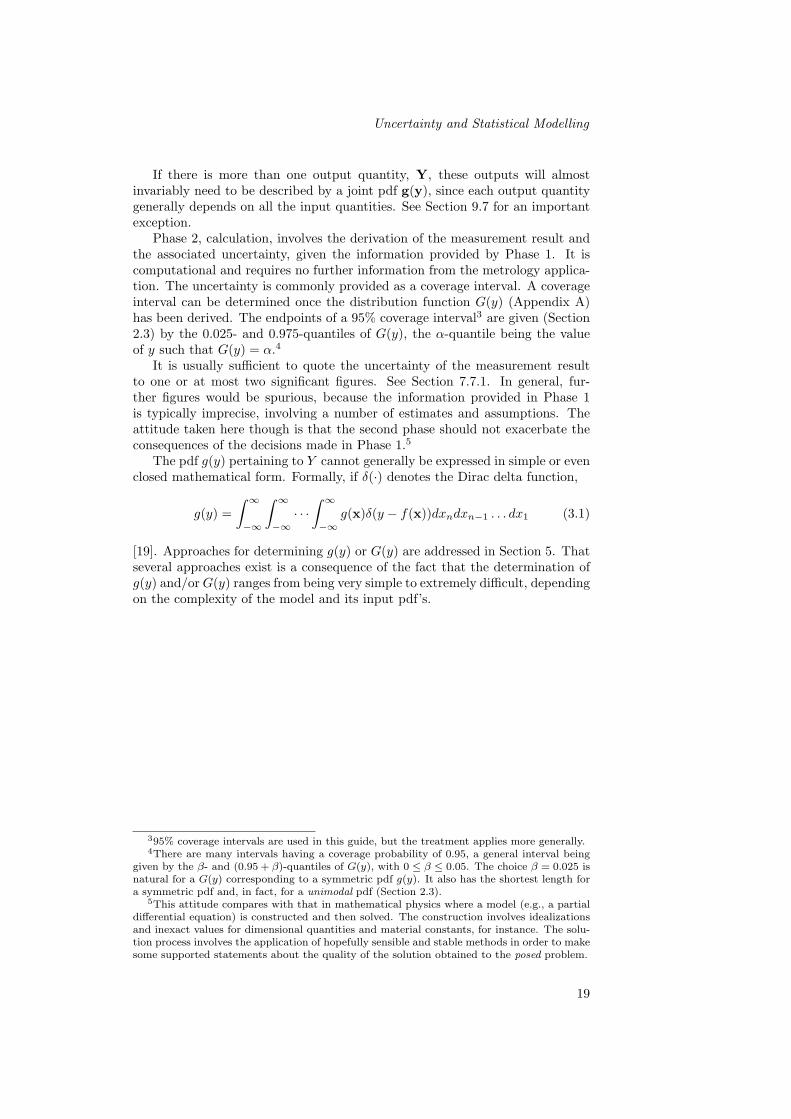
If there is more than one output quantity, Y, these outputs will almostinvariably need to be described by a joint pdf g(y), since each output quantitygenerally depends on all the input quantities. See Section 9.7 for an importantexception.
Phase 2, calculation, involves the derivation of the measurement result andthe associated uncertainty, given the information provided by Phase 1. It iscomputational and requires no further information from the metrology applica-tion. The uncertainty is commonly provided as a coverage interval. A coverageinterval can be determined once the distribution function G(y) (Appendix A)has been derived. The endpoints of a 95% coverage interval3 are given (Section2.3) by the 0.025- and 0.975-quantiles of G(y), the α-quantile being the valueof y such that G(y) = α.4
It is usually sufficient to quote the uncertainty of the measurement resultto one or at most two significant figures. See Section 7.7.1. In general, fur-ther figures would be spurious, because the information provided in Phase 1is typically imprecise, involving a number of estimates and assumptions. Theattitude taken here though is that the second phase should not exacerbate theconsequences of the decisions made in Phase 1.5
The pdf g(y) pertaining to Y cannot generally be expressed in simple or evenclosed mathematical form. Formally, if δ(·) denotes the Dirac delta function,
g(y) =∫ ∞
−∞
∫ ∞
−∞· · ·
∫ ∞
−∞g(x)δ(y − f(x))dxndxn−1 . . . dx1 (3.1)
[19]. Approaches for determining g(y) or G(y) are addressed in Section 5. Thatseveral approaches exist is a consequence of the fact that the determination ofg(y) and/or G(y) ranges from being very simple to extremely difficult, dependingon the complexity of the model and its input pdf’s.
395% coverage intervals are used in this guide, but the treatment applies more generally.4There are many intervals having a coverage probability of 0.95, a general interval being
given by the β- and (0.95 + β)-quantiles of G(y), with 0 ≤ β ≤ 0.05. The choice β = 0.025 isnatural for a G(y) corresponding to a symmetric pdf g(y). It also has the shortest length fora symmetric pdf and, in fact, for a unimodal pdf (Section 2.3).
5This attitude compares with that in mathematical physics where a model (e.g., a partialdifferential equation) is constructed and then solved. The construction involves idealizationsand inexact values for dimensional quantities and material constants, for instance. The solu-tion process involves the application of hopefully sensible and stable methods in order to makesome supported statements about the quality of the solution obtained to the posed problem.
19

Software Support for Metrology Best Practice Guide No. 6
Chapter 4
The main stages inuncertainty evaluation
In this guide, uncertainty evaluation is regarded as consisting of the two mainphases indicated in Chapter 3.1.
Phase 1, formulation, consists of providing the model and quantifying thepdf’s of the model input quantities. The constituent parts of Phase 1 are thethree steps
1. Statistical modelling.
2. Input-output modelling.
3. Assignment of probability density functions to the input quantities.
Phase 2, calculation, consists of deriving the measurement result and itsuncertainty, given the information provided by Phase 1. The constituent partsof Phase 2 are the two steps
1. Determination of the probability density function of the output quantity.
2. Provision of a coverage interval for the measurand.
4.1 Statistical modelling
Statistical modelling can be beneficial when a model is complicated, but isnot always needed for simpler models. It is concerned with developing therelationships between the measurements made, the measurands and the errorsof measurement.
Example 3 Straight-line calibration
A common example of statistical modelling arises when fitting a calibrationcurve to data, representing, say, the manner in which displacement varies withtemperature. The input quantities consist, for i = 1, . . . , n, say, of a measuredvalue xi of a response variable x corresponding to the value ti of a control orindependent variable t.
20

Uncertainty and Statistical Modelling
Consider a situation in which the ti are known with negligible error and xi
has error ei. Suppose that the nature of the calibration is such that a straight-line calibration curve y = a1 + a2x provides an adequate realization. Then, aspart of the statistical modelling process [22], the equations
xi = a1 + a2ti + ei, i = 1, . . . , n, (4.1)
relate the observations xi to the calibration parameters a1 (intercept) and a2
(gradient) of the line and the errors ei in the measurements.In order to establish values for a1 and a2 it is necessary to make an appro-
priate assumption about the nature of the errors ei [22]. For instance, if theycan be regarded as realizations of independent, identically distributed Gaussianvariables, the best unbiased estimate of the parameters is given by least squares.Specifically, a1 and a2 are given by minimizing the sum of the squares of thedeviations xi − a1 − a2ti, over i = 1, . . . , n, with respect to a1 and a2, viz.,
mina1,a2
n∑i=1
(xi − a1 − a2ti)2.
The model equations (4.1), with the solution criterion (least-squares), constitutethe results of the statistical modelling process for this example.
There may be additional criteria. For instance, a calibration line with anegative gradient may make no sense in a situation where the gradient representsa physical parameter whose “true” value must always be greater than or equalto zero (or some other specified constant value). The overall criterion in thiscase would be to minimize the above sum of squares with respect to a1 anda2, as before, with the condition that a2 ≥ 0. This problem is an example of aconstrained least-squares problem, for which sound algorithms exist [22]. In thissimple case, however, the problem can be solved more easily for the parameters,but the uncertainties associated with a1 and a2 require special consideration.See the example in Section 9.6.
Appendix B discusses some of the modelling issues associated with the sta-tistical modelling approach of this section and the input-output modelling ap-proach of the next.
4.2 Input-output modelling
Input-output modelling is the determination of the model required by the GUM,also termed here the GUM model, in its approach to uncertainty evaluation and,as indicated in Section 3.1, also in this guide. An input-output model can bederived from a statistical model or formed directly.
In the GUM [1] a measurement system is modelled, as in Section 3.1, bya functional relationship between measured or influence quantities (the inputquantities) X = (X1, . . . , Xn)T and the measurand (the output quantity) Y inthe form
Y = f(X). (4.2)
In practice this functional relationship does not apply directly to all measure-ment systems encountered, but may instead (a) take the form of an implicit rela-tionship, h(Y,X) = 0, (b) involve a number of measurands Y = (Y1, . . . , Ym)T,
21
Software Support for Metrology Best Practice Guide No. 6
or (c) involve complex-valued quantities. Section 6 is concerned with the man-ner in which each model type within this classification can be treated within a“GUM” setting. Here, the concern is with the basic form (4.2).
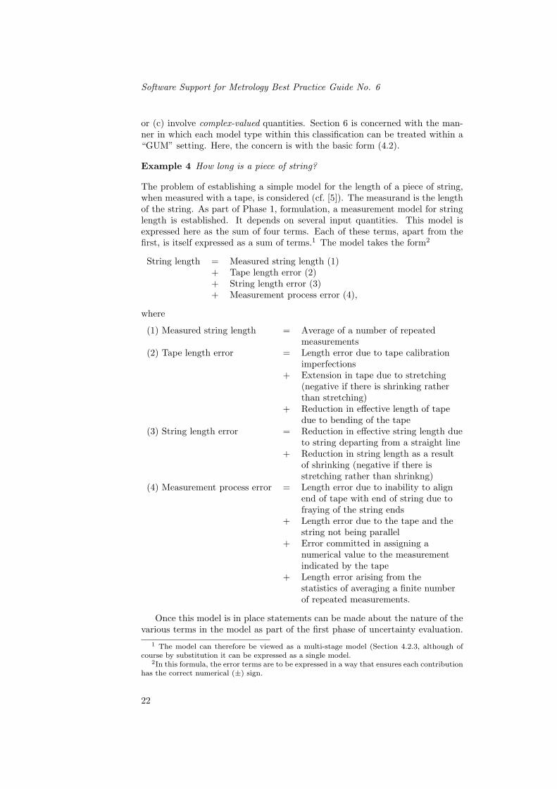
Example 4 How long is a piece of string?
The problem of establishing a simple model for the length of a piece of string,when measured with a tape, is considered (cf. [5]). The measurand is the lengthof the string. As part of Phase 1, formulation, a measurement model for stringlength is established. It depends on several input quantities. This model isexpressed here as the sum of four terms. Each of these terms, apart from thefirst, is itself expressed as a sum of terms.1 The model takes the form2
String length = Measured string length (1)+ Tape length error (2)+ String length error (3)+ Measurement process error (4),
where
(1) Measured string length = Average of a number of repeatedmeasurements
(2) Tape length error = Length error due to tape calibrationimperfections
+ Extension in tape due to stretching(negative if there is shrinking ratherthan stretching)
+ Reduction in effective length of tapedue to bending of the tape
(3) String length error = Reduction in effective string length dueto string departing from a straight line
+ Reduction in string length as a resultof shrinking (negative if there isstretching rather than shrinkng)
(4) Measurement process error = Length error due to inability to alignend of tape with end of string due tofraying of the string ends
+ Length error due to the tape and thestring not being parallel
+ Error committed in assigning anumerical value to the measurementindicated by the tape
+ Length error arising from thestatistics of averaging a finite numberof repeated measurements.
Once this model is in place statements can be made about the nature of thevarious terms in the model as part of the first phase of uncertainty evaluation.
1 The model can therefore be viewed as a multi-stage model (Section 4.2.3, although ofcourse by substitution it can be expressed as a single model.
2In this formula, the error terms are to be expressed in a way that ensures each contributionhas the correct numerical (±) sign.
22

Uncertainty and Statistical Modelling
Phase 2 can then be carried out to calculate the required uncertainty in themeasured length.
There may be some statistical modelling issues in assigning pdf’s to the inputquantities. For instance, a Student’s-t distribution would probably be assignedto the measured string length (1), based on the mean and standard deviation ofthe repeated measurements, with a number of degrees of freedom one less thanthe number of measurements. As another instance, for tape bending, this effectcan be approximated by a χ2 variable3 which does not, as required, have zeromean, since the minimum effect of tape bending on the measurand is zero.
Example 5 Straight-line calibration (re-visited)
For the straight-line calibration example of Section 4.1 (Example 3), the GUMmodel constitutes a formula or prescription (not in general necessarily explicit inform) derived from the results of the statistical modelling process. Specifically,the measurement results a = (a1, a2)T are given in terms of the input quantitiesx = (x1, . . . , xn)T by an equation of the form
Ha = q. (4.3)
(Compare [22], [1, Clause H.3].) Here, H is a 2× 2 matrix that depends on thevalues of the ti, and q a 2 × 1 vector that depends on the values of the ti andthe xi.
By expressing this equation as the formula
a = H−1q, (4.4)
a GUM model for the parameters of the calibration line is obtained. It is, atleast superficially, an explicit expression4 for the measurement result a. Theform (4.3) is also a GUM model, with the measurement result defined implicitlyby the equation (Section 6).
4.2.1 Correlated model parameters
In a range of circumstances some choice is possible regarding the manner inwhich the input quantities to the model is provided. A group of input quantitiescan be correlated in that each depends on a common effect. It may be possibleto re-express such input quantities so that the common effect appears explicitlyas a further input quantity. By doing so, this cause of correlation is eliminated,with the potential for a simplification of the analysis. See GUM Clause F.1.2.4.Also, an example in mass comparison [2] illustrates the principle.
3This degree of sophistication would not be warranted when measuring the length of apiece of string. It can be important in other applications.
4The expression is termed superficially explicit, since the determination of a via a formalmatrix inversion is not recommended [22]. The form (4.4), or forms like it in other such appli-cations, should not be regarded as an implementable formula [22]. Rather, numerically stablematrix factorization algorithms [35] should be employed. This point is not purely academic.The instabilities introduced by inferior numerical solution algorithms can themselves be anappreciable source of uncertainty. It is not straightforward to quantify this effect.
23

Software Support for Metrology Best Practice Guide No. 6
An example of this approach, in the context of measuring the sides of aright-angled triangle, is given in Section 9.4.
In general, the use of modelling principles, before uncertainties are assigned,is often helpful in understanding correlation effects.
4.2.2 Constrained uncertainty evaluation
Constrained uncertainty evaluations arise as a consequence of physical limitsor conditions associated with the measurands or the model input quantities.Instances include chemical concentrations, departures from perfect form in di-mensional metrology and limits of detection.
When chemical concentrations are measured, it will be appropriate to ensurethat in cases where all constituent parts are measured the estimates of themeasurands sum to unity (or 100%). The associated estimates will inevitablybe correlated even if the raw measurements have mutually independent errors.
In assessing the departure from perfect form in dimensional metrology, themeasurand is a quantity such as flatness, roundness, perpendicularity, concen-tricity, etc. These quantities are defined as the unsigned departure, assessedin an unambiguously defined way, of a real feature from an ideal feature, andare often very small, but nonzero. Any uncertainty statement associated withsuch a measurand that is based on a pdf that can embrace zero is physicallyunrealistic. Such a pdf is invariably asymmetric.
In triangulation, photogrammetry and similar applications, using theodo-lites, laser interferometers and metric cameras, redundancy of measurementensures that improved uncertainties are obtained compared with the use of anear-minimal number of measurements. The measurands, point co-ordinates,distances, etc. are interrelated by equality conditions deducible from geometri-cal considerations.
Within analytical chemistry, measurements of, e.g., trace elements, are madeat the limit of detection. At this limit the measurement uncertainty is compa-rable to the magnitude of the measurement itself. This situation has aspects incommon with that in dimensional metrology above, although there are appre-ciable contextual differences.
The Eurachem Guide to quantifying uncertainty in analytical measurementstates
[32, Appendix F] At low concentrations, an increasing variety ofeffects becomes important, including, for example,
• the presence of noise or unstable baselines,
• the contribution of interferences in the (gross) signal
• . . .
Because of such effects, as analyte concentrations drop, the rela-tive uncertainty associated with the result tends to increase, first toa substantial fraction of the result and finally to the point wherethe (symmetric) uncertainty interval includes zero. This region istypically associated with the practical limit of detection for a givenmethod.
. . .
24

Uncertainty and Statistical Modelling
Ideally, therefore, quantitative measurements should not be made inthis region. Nevertheless, so many materials are important at verylow levels that it is inevitable that measurements must be made, andresults reported, in this region. . . . The ISO Guide to the Expressionof Uncertainty in Measurement does not give explicit instructionsfor the estimation of uncertainty when the results are small and theuncertainties large compared to the results. Indeed, the basic formof the ‘law of propagation of uncertainties’ . . . may cease to applyaccurately in this region; one assumption on which the calculationis based is that the uncertainty is small relative to the value ofthe measurand. An additional, if philosophical, difficulty followsfrom the definition of uncertainty given by the ISO Guide: thoughnegative observations are quite possible, and even common in thisregion, an implied dispersion including values below zero cannotbe “reasonably ascribed to the value of the measurand” when themeasurand is a concentration, because concentrations themselvescannot be negative.
. . .
Observations are not often constrained by the same fundamentallimits that apply to real concentrations. For example, it is perfectlysensible to report an ‘observed concentration’, that is, an estimatebelow zero. It is equally sensible to speak of a dispersion of possibleobservations which extends into the same region. For example, whenperforming an unbiased measurement on a sample with no analytepresent, one should see about half of the observations falling belowzero. In other words, reports like
observed concentration = 2.4± 8 mg l−1
observed concentration = −4.2± 8 mg l−1
are not only possible; they should be seen as valid statements.
. . .
It is the view of the authors of this guide that these statements by Eurachemare sound. However, this guide takes a further step, related to modelling themeasurement and through the use of the model defining and making a statementabout the measurand, as opposed to the observations. Because a (simple) modelis established, this step arguably exhibits even closer consistency with the GUM.
The Eurachem statements stress that observations are not often constrainedby the same fundamental limits that apply to real concentrations. It is henceappropriate to demand that the measurand, defined to be the real analyte con-centration (or its counterpart in other applications) should be constrained tobe non-negative. Also, the observations should not and cannot be constrained,because they are the values actually delivered by the measurement method.Further, again consistent with the Eurachem considerations, assign a pdf tothe input quantity, viz., a best (unconstrained) estimate of the analyte con-centration, that is symmetric about that value. Thus, the input, X, say, isunconstrained analyte concentration with a symmetric pdf, and the output, Y ,say, real analyte concentration, with a pdf to be determined.
25

Software Support for Metrology Best Practice Guide No. 6
In terms of these considerations an appropriate GUM model is5
Y = max(X, 0). (4.5)
The rationale behind this simple choice of model is as follows. Should the meanx of the observations prove to be non-negative, it would naturally be taken asthe estimate of the measurand Y . Such a value would conventionally be usedat points removed from the limit of detection. Should x prove to be negative,it cannot be used as a physically feasible estimate of Y , since by definition Yis the real analyte concentration and hence non-negative. Taking y = 0 in thiscase is the optimal compromise between the observed values and feasibility (theclosest feasible value to the mean observation).
An example illustrating the use of this model is given in Section 9.5.
4.2.3 Multi-stage models
Multi-stage models are widespread in metrology. Even the string example (Sec-tion 4.2, Example 4) can be interpreted this way. Any situation in which theresults and uncertainties from one evaluation become the input quantities andassociated uncertainties to a subsequent stage constitute (part of) a multi-stagemodel. Within a model there are frequently sub-models, and therefore multi-staging arises also in this context. Examples abound, especially with calibration.
In the first stage of a multi-stage model, the metrologist is responsible forproviding all the input quantities. In subsequent stages, the input quantitiesconstitute some or all of the output quantities from previous stages plus, possi-bly, further input quantities from the metrologist.
Example 6 Example of a multi-stage model, in calibration
An example of a multi-stage model occurs regularly in calibration, when it isnecessary to establish and use a calibration curve. The following description is inthe context of Mainstream GUM. There would be an analogous description forcircumstances where it was necessary to avoid the Mainstream GUM limitationsand perhaps use MCS instead.
Stage 1 involves analysing measurement data that is a function of a secondvariable, e.g., displacement as a function of applied force. The displacement val-ues, and perhaps the values of the applied force, if they are not known accurately,constitute the (first-stage) model input quantities. The associated uncertainties,and covariances, if relevant, would be assigned. The model specifies the processof fitting a calibration curve to the data to provide the coefficients or parame-ters of the curve. These parameters constitute the model output quantities. Ifthere is more than parameter (the usual case), their values will almost invariablybe correlated, since each parameter will generally be a function of the (same)input data. Thus, the output quantities will have an associated non-diagonalcovariance matrix.
Stage 2 involves using the output quantities from Stage 1, viz., the curveparameters and their covariance matrix, as input quantities to a model thatconstitutes a rule for evaluating the calibration curve for appropriate values of
5Related considerations [46, p129] show that if an observation v is N(θ, 1) distributed, i.e.,drawn from a Gaussian distribution with mean zero and standard deviation unity, but θ ≥ 0,the maximum likelihood estimate of θ is max(v, θ).
26

Uncertainty and Statistical Modelling
the argument (force in the above instance).6 The output quantities will be thevalues of the curve at these designated points, together with their associatedcovariance matrix. Again, because these curve values all depend in general on allthe inputs, the curve parameters, this covariance matrix will be non-diagonal.
There may be no further stage, since the “interpolated” values provided bythe calibration curve may be the primary requirement.
Otherwise, Stage 3 will be the use of the curve values obtained in Stage 2to provide further measurement results. As an example, take the area under(a specified portion of) the calibration curve. Suppose that this area is to bedetermined by numerical quadrature because of the impossibility of carryingout the integration analytically. This result can typically be expressed as alinear combination of the curve values provided as input quantities. As anotherinstance, if more than one measurement result is required, e.g., estimates ofgradients to the curve at various points, these again can typically be expressedas linear combinations of the curve values. They will, for similar reasons tothose above, have a non-diagonal covariance matrix.
The concepts described in Chapter 6 can be applied to the above stages. Thevarious categories within the classification of that chapter would relate to thevarious types of calibration model, depending on whether it can be expressedexplicitly or implicitly or is real-valued or complex-valued. The model is almostalways multivariate in the sense of Chapter 6, i.e., it has more than one output.
4.3 Assignment of the input probability densityfunctions
The provision of input probability density functions (pdf’s) requires the assign-ment of appropriate statistical distributions (Gaussian, uniform, etc.) to themodel input quantities. It can be a challenging step in the formulation stage,Phase 1, of uncertainty evaluation. Valuable guidance is given in the GUM onthis matter. Additional aspects are considered here.
Sometimes these input pdf’s will be the result of a previous “uncertaintycalculation” within the context of a multi-stage model (Section 4.2.3).
In the above straight-line calibration example (Section 4.1, Example 3, andSection 4.2, Example 5), the pdf for each input quantity would have been takenas Gaussian, under the assumption that this knowledge of the errors in themeasurement process was available. There would be other types of measurementfor which the errors would be expected to be Poissonian, for example. Thereare many other types of measurement error.
Information concerning the underlying distribution should be deduced in anyone instance from all the knowledge that can economically be brought to bear(Section D.2).
6In many situations, it is necessary to use the calibration curve inversely. Typically, thedata in Stage 1 represents a set of standards, e.g., established responses to specified concen-trations. At Stage 2, it is required to use the calibration curve to determine the concentrationcorresponding to to an observed response. The mathematical function representing the curvethen constitutes an implicit model (Section 6.2.3) (e.g., if the calibration curve is a fifh-degreepolynomial).
27

Software Support for Metrology Best Practice Guide No. 6
There is an important class of metrology problems, viz., calibration as aboveor generally the analysis of experimental data. Suppose that there is a largenumber of “similar” measurements, such as in the straight-line calibration ex-ample in Section 4.1. Suppose also that the errors in these measurements canbe taken as uncorrelated. For a calibration function that can be expressed asa linear combination of calibration parameters, as above, these parameters canformally be written as a linear combination of the measured values. For the largenumber of measurements envisaged, the statistics of the situation are such thatalmost regardless of the nature of the distribution of the errors in the measure-ments, a linear combination of the measurements, as here, can be expected tohave essentially a Gaussian distribution, as a consequence of the Central LimitTheorem [51, p165]. When there are several such parameters (output quanti-ties) they will almost invariably be correlated, since each is a linear combinationof the input quantities. These paramaters would be described by a multivariate(joint) Gaussian distribution. See Section 4.3.2.
The straight line above would have an intercept and a gradient that arecorrelated.7
Even if the calibration function depends nonlinearly on its parameters, bylinearizing this function about the solution values of the parameters, to firstorder similar considerations apply as in the linear case [22]. In cases of doubt thevalidation procedures of Section 8 should be undertaken to determine whetherlinearization is justified.
The GUM [1] discriminates between the Type A evaluation of uncertainty—that based on statistical means—and the Type B evaluation of uncertainty—that based on non-statistical means. Although this terminology is sometimesused in this guide for alignment with the GUM, no great distinction is madehere, since all types of uncertainties can be classified by appealing to a unifyingprinciple (Section D.2). It is sometimes more useful to examine the distinctionbetween errors in a measurement that can be regarded as random and thosethat can be regarded as systematic.8 In some instances a systematic error canbe treated as a bias and handled as part of statistical modelling (Sections 4.1and 9.4).
Recommended assignments for Type A evaluations of uncertainty for threeimportant types of input quantity follow. They are based on the applicationof the Principle of Maximum Entropy (Section D.2). For each type the assign-ment applies on the condition that no information other than that specified isavailable. A “small number” of repeated observations is taken as ten or fewer.A “large number” is taken as greater than 20.
7It is possible in some applications such as this one to re-express (re-parametrise) thestraight line such that its parameters are uncorrelated [22]. Also see Section 4.2.1. Theexample in Clause H.3 of the GUM illustrates this point. Such re-parametrisation is not alwaysa practical proposition, however, because of the conflict between a numerically or statisticallyconvenient representation and the requirements of the application. However, the possibility ofre-parametrization should always be considered carefully for at least two reasons. One reasonis that the result corresponding to a sound parametrization can be obtained in a numericallystable manner [22], whereas a poor parametrization can lead to numerically suspect results.Another reason is that a poor parametrization leads to artificially large correlations in theoutput quantities. Decisions about the natural correlation present in the results cannot bemade in terms of these induced correlation effects.
8The subdivision into Type A and Type B evaluations of uncertainty will correspond insome instances to random and systematic effects, respectively, but not in all circumstances.
28

Uncertainty and Statistical Modelling
A small number of observations. The small number of repeated observa-tion is regarded as being drawn from an unknown distribution. Take themean and standard deviation of the mean. Assign a Gaussian pdf withthese parameters to the input quantity.
A small number of observations drawn from a Gaussian distribution.The small number of repeated observation is regarded as being drawn froma Gaussian distribution. Take the mean and standard deviation of themean. Assign a Student’s-t pdf with these parameters, with a number ofdegrees of freedom one less than the number of observations, to the inputquantity.
A large number of observations. A different attitude can legitimately betaken if a set of repeated observations is reasonably large. The observa-tions, when portrayed as a histogram, for instance, might indicate featuressuch as asymmetry or bimodality. If no additional information is available,rather than using the PME, the data itself can be used to “define” its ownpdf. Specifically, the pdf is given by assigning a probability 1/q, where qis the number of observations, to each value of the input quantity that isequal to one of these observations, and zero probability to all other valuesof the input quantity. Sampling from the pdf would take place simply byselecting a data value at random, with equal probability attached to allvalues. Any value selected is replaced before a further value is sampled.
An intermediate number of observations. The treatment of an interme-diate number of observations is more problematical. It will be adressed ina future edition of this guide.
4.3.1 Univariate Gaussian distribution
There are many circumstances where measurements contain errors that stemfrom a large number of sources and no one contribution dominates. In thesesituations it is reasonable to regard the measurements as having Gaussian errors.One common instance is a parameter arising from least-squares fitting (Section4.3).
The (univariate) Gaussian or normal distribution with mean µ and standarddeviation σ in the variable X has the pdf
g(x) =1
σ√
2πexp
−(x− µ)2/(2σ2)
, −∞ < x < ∞.
The standardized Gaussian distribution in the variable Z, with zero mean andunit standard deviation, is
φ(z) =1√2π
exp(−z2/2), −∞ < z < ∞.
Its distribution function, denoted by Φ(z), is
Φ(z) =∫ z
−∞φ(v)dv.
29
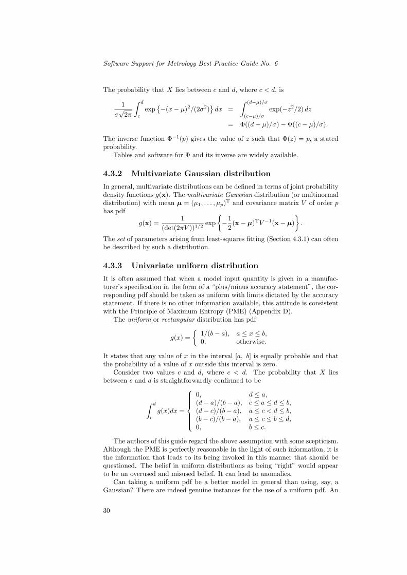
Software Support for Metrology Best Practice Guide No. 6
The probability that X lies between c and d, where c < d, is
1σ√
2π
∫ d
c
exp−(x− µ)2/(2σ2)
dx =
∫ (d−µ)/σ
(c−µ)/σ
exp(−z2/2) dz
= Φ((d− µ)/σ)− Φ((c− µ)/σ).
The inverse function Φ−1(p) gives the value of z such that Φ(z) = p, a statedprobability.
Tables and software for Φ and its inverse are widely available.
4.3.2 Multivariate Gaussian distribution
In general, multivariate distributions can be defined in terms of joint probabilitydensity functions g(x). The multivariate Gaussian distribution (or multinormaldistribution) with mean µ = (µ1, . . . , µp)T and covariance matrix V of order phas pdf
g(x) =1
(det(2πV ))1/2exp
−1
2(x− µ)TV −1(x− µ)
.
The set of parameters arising from least-squares fitting (Section 4.3.1) can oftenbe described by such a distribution.
4.3.3 Univariate uniform distribution
It is often assumed that when a model input quantity is given in a manufac-turer’s specification in the form of a “plus/minus accuracy statement”, the cor-responding pdf should be taken as uniform with limits dictated by the accuracystatement. If there is no other information available, this attitude is consistentwith the Principle of Maximum Entropy (PME) (Appendix D).
The uniform or rectangular distribution has pdf
g(x) =
1/(b− a), a ≤ x ≤ b,0, otherwise.
It states that any value of x in the interval [a, b] is equally probable and thatthe probability of a value of x outside this interval is zero.
Consider two values c and d, where c < d. The probability that X liesbetween c and d is straightforwardly confirmed to be
∫ d
c
g(x)dx =
0, d ≤ a,(d− a)/(b− a), c ≤ a ≤ d ≤ b,(d− c)/(b− a), a ≤ c < d ≤ b,(b− c)/(b− a), a ≤ c ≤ b ≤ d,0, b ≤ c.
The authors of this guide regard the above assumption with some scepticism.Although the PME is perfectly reasonable in the light of such information, it isthe information that leads to its being invoked in this manner that should bequestioned. The belief in uniform distributions as being “right” would appearto be an overused and misused belief. It can lead to anomalies.
Can taking a uniform pdf be a better model in general than using, say, aGaussian? There are indeed genuine instances for the use of a uniform pdf. An
30

Uncertainty and Statistical Modelling
1 1.02 1.04 1.06 1.08 1.1−3
−2
−1
0
1
2
3
4x 10
−3
Figure 4.1: The errors in successive values displayed by a simulated instrumenthaving a resolution of two decimal places. The values shown are the differencesbetween the values of sin t that would be displayed by the instrument and theactual values of sin t, for t = 1.00, 1.01, . . . , 1.10 radians.
example is the digital resolution of an instrument, in which the error can beregarded as being equally likely anywhere within plus or minus half a unit inthe last displayed digit.9
The quantization error in analogue to digital conversion also falls (with someexceptions) into this category. There would appear to be few other genuine ex-amples. It would be desirable, especially in a competitive environment or whenparticularly reliable uncertainty statements are required, to approach suppli-ers to relate the provided accuracy statement to the context in which it wasmade. The supplier might, for example, be speaking loosely, e.g., to imply a99% coverage interval, say, with the previously unmentioned information thatan underlying Gaussian pdf was reasonable. The contextual information mightrelate, for example, to reject rates in a production process.
Information is available [10] on a method for reducing the uncertainty as-sociated with instrument resolution when a series of observations is taken. Itinvolves randomizing the zero setting, where this is possible, before taking eachobservation. The mean of a set of q observed values so obtained can be expectedto have an uncertainty that is smaller than that of an individual observationby a factor of
√q. This result is to be compared with conventional repeated
observations in situations where the uncertainties are dominated by those ofthe instrument resolution: the mean of the observations has no better propertythan the individual observations.
9This statement is correct for a single reading. There are additional considerations fora sequence of readings corresponding to a slowly varying signal. The errors in the resolvedsequence are serially correlated as a consequence of the resolution of the instrument. Figure 4.1shows the errors in successive values displayed by a simulated instrument having a resolutionof two decimal places. The values shown are the differences between the values of sin t thatwould be displayed by the instrument and the actual values of sin t, for t = 1.00, 1.01, . . . , 1.10radians. Any analysis of such data that did not take account of the very obvious serialcorrelation would yield a flawed result. The effects of serial correlation depend on the relativesizes of the uncertainties in the signal, the instrument resolution and the magnitudes of thechanges in successive values of the signal (the last-mentioned item depending on the samplingrate). In hopefully many cases they will be negligible, but it is appropriate to establish whenthis is indeed the case. In the context of calibration it is stated [28], but the point is moregeneral, that the measurement uncertainty associated with the calibration of all low-resolutionindicating instruments is dominated by the finite resolution provided this resolution is the onlydominant source in the uncertainty budget.
31
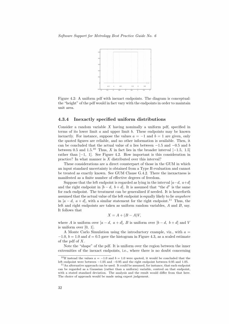
Software Support for Metrology Best Practice Guide No. 6
−2 −1.5 −1 −0.5 0 0.5 1 1.5 2−0.1
0
0.1
0.2
0.3
0.4
0.5
a ba−d a+d b−d b+d
X
Figure 4.2: A uniform pdf with inexact endpoints. The diagram is conceptual:the “height” of the pdf would in fact vary with the endpoints in order to maintainunit area.
4.3.4 Inexactly specified uniform distributions
Consider a random variable X having nominally a uniform pdf, specified interms of its lower limit a and upper limit b. These endpoints may be knowninexactly. For instance, suppose the values a = −1 and b = 1 are given, onlythe quoted figures are reliable, and no other information is available. Then, itcan be concluded that the actual value of a lies between −1.5 and −0.5 and bbetween 0.5 and 1.5.10 Thus, X in fact lies in the broader interval [−1.5, 1.5]rather than [−1, 1]. See Figure 4.2. How important is this consideration inpractice? In what manner is X distributed over this interval?
These considerations are a direct counterpart of those in the GUM in whichan input standard uncertainty is obtained from a Type B evaluation and cannotbe treated as exactly known. See GUM Clause G.4.2. There the inexactness ismanifested as a finite number of effective degrees of freedom.
Suppose that the left endpoint is regarded as lying in the interval [a−d, a+d]and the right endpoint in [b− d, b + d]. It is assumed that “the d” is the samefor each endpoint. The treatment can be generalised if needed. It is henceforthassumed that the actual value of the left endpoint is equally likely to lie anywherein [a − d, a + d], with a similar statement for the right endpoint.11 Thus, theleft and right endpoints are taken as uniform random variables, A and B, say.It follows that
X = A + (B −A)V,
where A is uniform over [a− d, a + d], B is uniform over [b − d, b + d] and Vis uniform over [0, 1].
A Monte Carlo Simulation using the introductory example, viz., with a =−1.0, b = 1.0 and d = 0.5 gave the histogram in Figure 4.3, as a scaled estimateof the pdf of X.
Note the “shape” of the pdf. It is uniform over the region between the innerextremities of the inexact endpoints, i.e., where there is no doubt concerning
10If instead the values a = −1.0 and b = 1.0 were quoted, it would be concluded that theleft endpoint were between −1.05 and −0.95 and the right endpoint between 0.95 and 1.05.
11An alternative approach can be used. It could be assumed, for instance, that each endpointcan be regarded as a Gaussian (rather than a uniform) variable, centred on that endpoint,with a stated standard deviation. The analysis and the result would differ from that here.The choice of approach would be made using expert judgement.
32

Uncertainty and Statistical Modelling
−1.5 −1 −0.5 0 0.5 1 1.50
0.5
1
1.5
2
2.5
3x 10
4
Figure 4.3: A histogram produced using Monte Carlo Simulation for the modelX = A + (B − A)V , where A is uniform over [a− d, a + d], B is uniform over[b− d, b + d] and V is uniform over [0, 1], with a = −1.0, b = 1.0 and d = 0.5.Figure 4.2 refers. The histogram provides a scaled estimate of the pdf of X.It corresponds to an input quantity that is defined by a uniform distributionbetween inexact limits, theirselves being represented by uniform distributions.
−1.5 −1 −0.5 0 0.5 1 1.50
0.5
1
1.5
2
2.5
3x 10
4
Figure 4.4: As Figure 4.3 except that the endpoints are related as described inthe text.
their location. Between the inner and outer extremities it reduces from theuniform height to zero in what is approximately a quadratic manner. Beyond theouter extremities the pdf is zero. The piecewise nature of the pdf is comparableto that for the sum of uniform pdf’s, where the pieces form polynomial segments[26].
The standard deviation of X, assuming the exactness of the endpoints (equiv-alent to taking d = 0), is 1/
√3 = 0.577. That for the above finite value of d
is 0.625. As might be expected, the inexactness of the endpoints increases thevalue. The extent to which this increase (8%) is important depends on circum-stances.
There will be situations where the inexact endpoints would be expected to“move together”, i.e., the knowledge of one of them would imply the other. Inthis circumstance the pdf of X is slightly different. See Figure 4.4. The standarddeviation of X is now 0.600 (a 4% increase over that for d = 0), roughly halfwaybetween that for the above pdf and the pure uniform pdf. The flanks of the pdfnow have greater curvature.
The final statement to be made here concerning uniform distributions withinexactly defined endpoints is that the effects of such endpoints on the evaluation
33

Software Support for Metrology Best Practice Guide No. 6
of uncertainty increase with the relative amount of inexactness. This pointis qualitatively consistent with the use of an effective number of degrees offreedom, as above, in the GUM. Increased inexactness will give rise to a smallernumber and yield greater uncertainty through a larger coverage factor from theStudent’s-t distribution.
The main message is that inexactness in the information that leads to assign-ing pdf’s not only modifies the forms of those pdf’s, but influences the relevantstandard deviations.
4.3.5 Taking account of the available information
It is beyond the scope, in this first edition of this best-practice guide, to statehow all information available can properly be taken into account. Some remarksare made, however, indicating how the Principle of Maximum Entropy can beused to advantage. A future edition will provide more details.
If a set of values, in the form of repeated observations, is available, and noother information is provided, the PME would mandate the use of a Gaussianpdf with mean and standard deviation deduced from the measurements.
If only a lower and an upper limit were available the PME would supportthe choice of a uniform pdf, as above.
Suppose a prior pdf, say a Gaussian, were available, perhaps from historicalinformation such as that obtained in previous calibrations. Suppose that furthermeasurements were available. The use of the PME would permit both sources ofinformation to be combined to deliver a Students-t pdf that could be expectedto be more reliable than the pdf from either source alone.
Suppose a prior uniform pdf were available, perhaps from sound knowledgeof limits, and that one measurement was made. From the PME, the uniformpdf that would be inferred from the limits alone would be modified by themeasurement. The GUM provides (in GUM Clause 4.3.8) the pdf in this case.
Other cases can be handled, and give superior results in general than iftreated without taking account of the available information. Such cases mayrequire the services of a statistician.
Appendix D considers some of the issues involved.It is relevant to note that in the context of Mainstream GUM, which works
only with the standard deviations (and the means) of the input pdf’s, the GUMstates
[GUM Clause E.4.2] When the standard uncertainty of an inputquantity cannot be evaluated by analysis of the results of an ad-equate number of repeated observations, a probability distributionmust be adopted based on knowledge that is much less extensivethan might be desirable. That does not, however, make the distri-bution invalid or unreal; like all probability distributions it is anexpression of what knowledge exists.
This attitude is consistent with a Bayesian view [65].
34

Uncertainty and Statistical Modelling
4.4 Determining the output probability densityfunction
The pdf of the output quantity is completely defined by the model together withthe assigned input pdf’s. Appropriate analysis or calculation is needed, however,to determine it. Chapter 5 covers candidate approaches for forming the outputpdf in the univariate case, and indicates its counterpart in the multivariate case.
4.5 Providing a coverage interval
The provision of a coverage interval is the use of the pdf of the output quantityto determine a lower limit and an upper limit of an interval that can be expectedto contain 95% (or some other specified proportion) of the values that can bereasonably be attributed to the measurand. See Chapter 5 for methods fordetermining the pdf of the output quantity. See Section 2.3 for information oncoverage intervals. Coverage intervals can be obtained objectively from a pdf.They can also be obtained from coverage factors and an assumption concerningthe pdf.
4.5.1 Coverage intervals from distribution functions
If the distribution function is known, a coverage interval can be obtained asindicated in Section 2.3.
4.5.2 Coverage intervals from coverage factors and an as-sumed form for the distribution function
The Mainstream GUM approach (see GUM Clause G.1.1) to determining acoverage interval is as follows. The aim (using the notation of the GUM) is toprovide, using the estimate y of the measurand Y and the standard uncertaintyu(y) of the estimate, an expanded uncertainty Up = kpu(y). With the estimatey, this value Up defines an interval [y−Up, y +Up] that has a specified coverageprobability p.
In summarizing its recommendations for determining this coverage interval,the GUM states:
[GUM Clause G.6.1] The coverage factor kp that provides an inter-val having a level of confidence p close to a specified level can onlybe found if there is extensive knowledge of the probability distribu-tion of each input quantity and if these distributions are combinedto obtain the distribution of the output quantity. The input esti-mates xi and and their standard uncertainties u(xi) by themselvesare inadequate for this purpose.
Further,
[GUM Clause G.6.2] Because the extensive computations required tocombine probability distributions are seldom justified by the extentand reliability of the available information, an approximation to thedistribution of the output quantity is acceptable. Because of the
35

Software Support for Metrology Best Practice Guide No. 6
Central Limit Theorem, it is usually sufficient to assume that theprobability distribution of (y − Y )/uC(y) is the t-distribution andtake kp = tp(νeff), with the t-factor based on an effective degreesof freedom νeff of uC(y) obtained from the Welch-Satterthwaite for-mula ...
The statement12 concerning the extensive computation to combine probabilitydistributions is no longer tenable, with PCs faster than 1 GHz being common-place. Unless the model is complicated, the determination of the pdf of theoutput quantity and hence the required coverage interval to the required num-ber of figures, can, with todays’ PCs, be carried out in computation times ofminutes or even seconds (Section 7.3.1).
4.5.3 An approximation is acceptable, but is it an accept-able approximation?
The statement from the GUM reproduced in Section 4.5.2 concerning the Cen-tral Limit Theorem demands investigation. It is accepted that it is usuallysufficient to assume that the output is distributed as Student’s-t. The difficultylies in deciding when this assumption can be made. The GUM offers no specificguidance in this regard. This document supports that approach when it can bejustified, but recommends that in any case of doubt the validation approach ofSection 8.2 should be employed.
However, the GUM does provide some advice regarding the circumstanceswhen Mainstream GUM can be expected to hold:
[GUM Clause 6.6] For many practical measurements in a broad rangeof fields, the following conditions prevail:
- the estimate y of the measurand Y is obtained from estimates xi ofa significant number of input quantities Xi that are describableby well-behaved probability distributions, such as the normaland rectangular distributions;
- the standard uncertainties u(xi) of these estimates, which maybe obtained from either Type A or Type B evaluations, con-tribute comparable amounts to the combined standard uncer-tainty uC(y) of the measurement result y;
- the linear approximation implied by the law of propagation ofuncertainty is adequate (see 5.1.2 and E.3.1);
- the uncertainty of uC(y) is reasonably small because its effectivedegrees of freedom νeff has a significant magnitude, say greaterthan 10.
Under these circumstances, the probability distribution character-ized by the measurement result and its combined standard uncer-tainty can be assumed to be normal because of the Central LimitTheorem; and uC(y) can be taken as a reasonably reliable estimateof the standard deviation of the normal distribution because of thesignificant size of νeff.
12The GUM uses the notation uC(y) for combined standard uncertainty, i.e., that associatedwith y. This guide simply uses u(y).
36

Uncertainty and Statistical Modelling
This advice is sound in a qualitative sense but, again, it is unclear when thecircumstances hold. The problem is that the distinction between Phase 1 andPhase 2 of uncertainty evaluation13, as indicated in Section 4, becomes blurred.The intention of the subdivision into the two phases is to permit all decisionsto be made in Phase 1 and the mechanical calculations to be made in Phase 2.
In terms of the set of conditions in GUM Clause 6.6, listed above, it is unclearwhat is meant by
• “a significant number of input quantities”
• “well-behaved probability distributions”
• the standard uncertainties of the xi contributing comparable amounts14
• the adequacy of linear approximation, and
• the output uncertainty being reasonably small.
The concern is that because none of these considerations is explicitly quanti-fied, different practitioners might adopt different interpretations of the samesituation, thus causing divergence of results.
Further, an approximation is acceptable, but is it an acceptable approxima-tion?
4.6 When the worst comes to the worst
Consider a situation in which no assumption is to be made about the pdf of theoutput quantity other than an estimate of its mean value y and the standarddeviation u(y) of this estimate. One reason for wishing to make no assumptionis that it may be difficult or impossible to obtain distributional informationabout some of the input quantities and it is deemed inappropriate to invoke thePrinciple of Maximum Entropy. In such a circumstance, a conservative estimateof a coverage interval can be obtained using some traditional results from thestatistical literature.15 Two results are possible. One result is general, applyingto all distributions. The other relates to instances in which one is prepared tomake a single assumption, viz., that the distribution is symmetric.
4.6.1 General distributions
Suppose that it is required to quote an uncertainty interval for the measurandY corresponding to a coverage probability of 95%, and that nothing is knownabout the distribution.
13The JCGM/WG1 has agreed that this distinction is useful. It will form part of a supple-mental guide being produced by JCGM/WG1.
14This statement is taken here to mean that the standard uncertainties of the input quan-tities, when scaled by the magnitudes of the corresponding sensitivity coefficients, contributecomparable amounts.
15Such an estimate is inconsistent with the intention of the GUM which promotes the useof a realistic coverage interval:
[GUM, Clause 0.4] . . . the ideal method for evaluating and expressing uncertaintyin measurement should be capable of readily providing such an interval, in par-ticular, one with a coverage probability or level of probability that correspondsin a realistic way with that required.
There may, however, be special situations where a conservative estimate is useful.
37

Software Support for Metrology Best Practice Guide No. 6
The coverage interval y ± ku(y), where k = 4.47, contains at least 95% ofthe distribution of y-values.
This result is derived from Chebyshev’s inequality which states that the prob-ability that Y lies in the interval y ± ku(y) is at least 1 − k−2. The value of kfor which 1− k−2 = 0.95 is 4.47. It is stressed that this result applies regardlessof the distribution. By its nature it cannot be as sharp as an interval derivedfrom knowledge of the pdf of y, e.g.,
• If Y is uniform this interval is y ± 1.65u(y)
• If Y is Gaussian it is y ± 1.96u(y).
The length of the interval derived from Chebyshev’s inequality is 2.7 times thelength of that for uniform Y and 2.3 times that for Gaussian Y .
Note. These results applies only if the number of degrees of freedom isinfinite, or in practice large. Otherwise, the k-factor becomes inflated, as in thecase of Student’s-t distribution [53].
4.6.2 Symmetric distributions
If it is known that the distribution is symmetric, tighter results based on Gauss’sinequality are possible.
The coverage interval y ± ku(y), where k = 2.98, contains at least 95% ofthe distribution of y-values.
Gauss’s inequality states that the probability that Y lies in the intervaly±ku(y) is at least 1− 4
9k−2. The value of k for which 1− 49k−2 = 0.95 is 2.98.
It is noted that this interval is only approximately 50% longer than thatwhen Y is Gaussian (Section 4.6.1).
Note. These results applies only if the number of degrees of freedom isinfinite, or in practice large. Otherwise, the k-factor becomes inflated, as in thecase of Student’s-t distribution.
4.6.3 Making stronger assumptions
Tighter, distribution-free, coverage intervals can be obtained if stronger assump-tions are made, such as unimodality (single-peakedness) as well as symmetry ofthe pdf.
38

Uncertainty and Statistical Modelling
Chapter 5
Candidate solutionapproaches
This chapter covers candidate solution processes for the calculation phase, Phase2, of the uncertainty evaluation problem formulated in Section 3.1. The start-ing point is (i) the availability of a model f or f that relates the input quan-tities X = (X1, . . . , Xn)T to the scalar measurand Y or vector measurandY = (Y1, . . . , Ym)T through Y = f(X) or Y = f(X), and (ii) assigned probabil-ity density functions (pdf’s) g1(X1), . . . , gn(Xn) for the input quantities. If theinput quantities are correlated, they will have a joint pdf.
It is required to determine the pdf g(Y ) for the output quantity y or the(joint) pdf g(Y) for Y.
Once g(Y ) has been obtained a 95% coverage interval for the (scalar) mea-surand Y can be derived. Once g(Y) has been obtained, a 95% coverage regionfor the (vector) measurand Y can be derived.
Three approaches to the determination of the output pdf for Y or Y areconsidered and contrasted:
1. Analytical methods
2. Mainstream GUM
3. Numerical methods.
All three approaches are consistent with the GUM. Mainstream GUM is theprocedure that is widely used and summarized in GUM Clause 8. Analyticalmethods and numerical methods fall in the category of “other analytical andnumerical methods” (GUM Clause G.1.5). Under the heading of “Analyticalmethods” below, mention is also made of “Approximate analytical methods”.
5.1 Analytical methods
Analytical methods to obtain the pdf of Y or Y are preferable in that they do notintroduce any approximation, but can be applied in relatively simple cases only.Their application may require the services of an expert. A treatment of suchmethods, based essentially on the use of formula (3.1) is available [26]. Instances
39

Software Support for Metrology Best Practice Guide No. 6
1 2 3−0.1
0
0.1
0.2
0.3
0.4
0.5
0.6
0 0.5 1
−0.2
0
0.2
0.4
0.6
0.8
1
1.2
1.4
1.6
1.8
Figure 5.1: A uniform probability density function (left) for the input X andthe corresponding probability density function for the output Y , where Y isrelated to X by the model Y = log(X).
that can be so handled include additive models, Y = a1X1 + . . . + anXn, whereall Xi are Gaussian or all are uniform. In the latter case, unless n is small, themultipliers ai must be equal and the semi-widths of the uniform pdf’s identical1
to avoid formidable algebra.
5.1.1 Single input quantity
The case of a single input quantity (n = 1) is amenable to analytic treatment [51,pp57-61]. If the model function f(X) is differentiable and strictly monotonic,Y has the pdf
g(y) = g(f−1(y))|d(f−1(y))/dy|. (5.1)
Example 7 A logarithmic transformation
If the model is Y = ln(X) with X having uniform pdf in [a, b], the applicationof Formula (5.1) gives
G(y) =
0, y ≤ ln(a),(exp(y)− a)/(b− a), ln(a) ≤ y ≤ ln(b),1, ln(b) ≤ y.
(cf. Section 4.3.5). Figure 5.1 depicts the uniform pdf (left) for X and thecorresponding pdf for Y in the case a = 1, b = 3.
This case is important in, say, electromagnetic compatibility measurement,where conversions are often carried out between quantities expressed in linearand decibel units using exponential or logarithmic transformations [62].
Example 8 A linear combination of Gaussian distributions
Suppose the model isY = a1X1 + · · ·+ anXn,
where a1, . . . , an are specified constants, and, for i = 1, . . . , n, Xi has a Gaussiandistribution with mean µi and standard deviation σi. Then Y has a Gaussian
1In this case Y is a B-spline with uniform knots [18].
40

Uncertainty and Statistical Modelling
- YA
AAA
Figure 5.2: The probability density function for the sum Y = X1 + X2 of twouniform distributions X1 and X2 of identical semi-widths.
distribution with mean µ = a1µ1 + · · ·+ anµn and standard deviation (a21σ
21 +
· · ·+ a2nσ2
n)1/2.
Example 9 The sum of two uniform distributions with the same semi-widths
Suppose the model isY = X1 + X2
and, for i = 1, 2, Xi has a uniform pdf with mean µi and semi-width a (and hencestandard deviation a/
√3). Then Y has a symmetric triangular pdf g(y) with
mean µ = µ1+µ2, semi-width 2a and standard deviation a√
2/3. Geometrically,this pdf, for the case µ1 + µ2 = 0, takes the form
g(y) =
0, y ≤ −2a,(2a + y)/(4a2), −2a ≤ y ≤ 0,(2a− y)/(4a2), 0 ≤ y ≤ 2a,0, 2a ≤ y.
For general µ1 and µ2, the pdf is the same, but centred on µ1 + µ2 rather thanzero. Geometrically, this pdf takes the form indicated in Figure 5.2.
Example 10 The sum of n uniform distributions of the same semi-width
Suppose the model isY = X1 + · · ·+ Xn
and, for i = 1, . . . , n, Xi has a uniform pdf with mean µi and semi-width a (andhence standard deviation a/
√3). Then Y is a B-spline of order n (degree n−1)
with mean µ = µ1 + · · ·+ µn and standard deviation a√
n/3.
Example 11 The sum of two uniform distributions of arbitrary semi-widths
Suppose the model isY = α1X1 + α2X2
and, for i = 1, 2, Xi has a uniform pdf with mean µi and semi-width ai (andhence standard deviation ai/
√3). Then Y has a symmetric trapezoidal pdf g(y)
with mean µ = α1µ1 + α2µ2, semi-width α1a1 + α2a2 and standard deviation(α2
1a21+α2
2a22)/31/2. Geometrically, this pdf takes the form indicated in Figure
5.3.
Analytical solutions in some other simple cases are available [26, 28].
41

Software Support for Metrology Best Practice Guide No. 6
- Y A
AAA
Figure 5.3: The probability density function for a general linear combinationY = α1X1 + α2X2 of two uniform distributions X1 and X2. It is symmetricabout its midpoint.
5.1.2 Approximate analytical methods
Approximate analytical methods are approaches that fall part-way between theanalytical methods of Section 5.1 and the numerical methods of Section 5.3.They are related to Mainstream GUM (Section 6), but take the analysis fur-ther in order to provide approximate analytical expressions for the pdf of theoutput quantity in cases where Gaussian or Student’s-t pdf’s obtained in theconventional way would be invalid.
A treatment [28] of some calibration examples using approximate analyticmethods provides output pdf’s in the form of
1. A uniform output pdf in the calibration of a hand-held digital multimeter,
2. A symmetric trapezoidal pdf in the calibration of a vernier caliper,
3. A further trapezoidal pdf in the calibration of a temperature block calibra-tor.
The first of these examples is used subsequently in this guide (Section 9.3)in the context of the MCS approach to uncertainty evaluation and the resultscompared with those of [28] and Mainstream GUM.
5.2 Mainstream GUM
The GUM makes the following statement about the pdf’s of the input quanti-ties:2
[GUM Clause 4.1.6] Each input estimate xi and its associated un-certainty u(xi) are obtained from a distribution of possible valuesof the input quantity Xi. This probability distribution may be fre-quency based, that is, based on a series of observations xi,k of Xi,or it may be an a priori distribution. Type A evaluations of stan-dard uncertainty components are founded on frequency distributionswhile Type B evaluations are founded on a priori distributions. Itmust be recognized that in both cases the distributions are modelsthat are used to represent the state of our knowledge.
2To this statement, the comment must be added that some pdf’s may be based on bothtypes of information, viz., prior knowledge and repeated observations. Evaluations of standarduncertainty in this setting are not purely Type A or Type B. The GUM gives one such instance(GUM Clause 4.3.8, Note 2.)
42

Uncertainty and Statistical Modelling
The intent of Mainstream GUM is to derive the parameters of a Gaussianor Student’s-t distribution that represents the output pdf g(y) given the pdf’sof the inputs Xi to the model.
For Mainstream GUM, the following steps constitute the calculation phase,Phase 2:
1. Obtain from the (joint) input pdf(s) the means x = (x1, . . . , xn)T and thestandard deviations u(x) = (u(x1), . . . , u(xn))T of the input quantities.
2. Form the covariances u(xi, xj) of the input quantities from the appropriatejoint pdf’s for any pair of correlated input quantities.
3. Form the partial derivatives of first order of the model with respect to theinput quantities. See Section 5.5.
4. Form numerically the (mean) measurement result by evaluating the modelat the estimates of the input quantities (the means of the input pdf’s).
5. Form the model sensitivities as the values of the partial derivatives eval-uated at these means. See Section 5.5.
6. Determine the combined standard uncertainty, viz., the standard devia-tion of the model output quantity, by combining the values of the inputstandard uncertainties, the input covariances and the model sensitivities(GUM Formula (13)). See Section 6.2.1.
7. Calculate ν, the effective number of degrees of freedom of the output quan-tity, using the Welch-Satterthwaite formula (GUM Equation (G.2b)).3
8. Compute the expanded uncertainty, and hence an interval having a stip-ulated coverage probability containing the measurand, by forming theappropriate multiple of the combined standard uncertainty under theassumption that the output is a Gaussian distribution (ν = ∞) or aStudent’s-t distribution (ν < ∞).
A review of the Mainstream GUM procedure is given in Section 5.4. Details,procedures and examples are given in Chapter 6.
5.3 Numerical methods
It would rarely be a practical proposition to use the integral expression (3.1) inSection 3.1 as the basis for the numerical determination of g(y), the pdf of theoutput quantity. A multivariate quadrature rule4 would need to be devised thatwas capable of delivering g(y) to a prescribed numerical accuracy for each choiceof y. Further, the quadrature rule would have to be applied at a sufficiently fineset of y-values to provide g(y) adequately.
3Mainstream GUM does not state how ν is to be calculated when the input quantities arecorrelated.
4A quadrature rule is a numerical integration procedure. Examples in the univariate caseare the trapezoidal rule and Simpson’s rule.
43

Software Support for Metrology Best Practice Guide No. 6
5.3.1 Monte Carlo Simulation
Rather than attempting to evaluate the integral (3.1), Monte Carlo Simulation(MCS) [4, 19, 21, 23, 54, 64] encompasses an entirely different approach, basedon the following considerations. The expected value of the output quantity Yis conventionally obtained by evaluating the model for the estimated (mean)values x1, . . . , xn of the input quantities to give the value y. However, sinceeach input quantity is described by a pdf rather than a single number, a valueas legitimate as its mean can be obtained by drawing a value at random fromthis function.
MCS operates in the following manner,5 based on this consideration. Gen-erate a value at random from the pdf for each input quantity and form thecorresponding value of the output, by evaluating the model for these values asinput quantities. Repeat this process many times, to obtain in all M , say, es-timates of the output quantity. According to the Central Limit Theorem [51,p169], the mean value y of the estimates of the output quantity obtained inthis manner converges as 1/M1/2, if the standard deviation u(y) of y exists.Irrespective of the dimensionality of the problem, i.e., the number n of inputquantities, it is (only) necessary to quadruple M in order to halve the expecteduncertainty in the estimate of u(y). Standard numerical quadrature would re-quire a factor of 2N/2 for this purpose. Thus, the basic concept of MCS hasreasonable convergence properties. It is straightforward to implement for simpleor even moderately complicated problems. Its general implementation requireseffort: see Section 7.7. A broad introduction to MCS is available [38], as is adiscussion on uncertainty propagation in Monte Carlo calculations [57].
Details, procedures and examples are given in Chapter 7.
5.4 Discussion of approaches
The approach used for any particular problem needs to be chosen with care. Asindicated, Mainstream GUM is the “method of choice” for many organizations.Analytical methods are in a sense ideal when applicable. Numerical methodsoffer flexibility. MCS is increasingly used by laboratories and industrial organi-zations. A more detailed comparison of the three approaches will be preparedas part of the SSf M programme (Section 1.1) and given in a future edition ofthis guide. Here, selected comments are made.
5.4.1 Conditions for Mainstream GUM
Mainstream GUM requires
1. The linearization of the model to be sufficiently accurate.6
2. The applicability of the Central Limit Theorem (GUM Clause G.2.1),implying the representativeness of g(y), the pdf of the output quantity,
5This description applies to a model with a single output quantity. For a multivariateproblem, additional considerations apply (Section 7.4).
6If the linearization of the model is not sufficiently accurate, the quality of the evaluateduncertainty is affected, as is the estimate of the measurand. The latter point may be less wellappreciated in some quarters. The bias so introduced into the estimate of the measurand isillustrated in Section 9.5, for example.
44

Uncertainty and Statistical Modelling
by a Gaussian or Student’s-t distribution with known mean and standarddeviation and, in the latter case, a known number ν of degrees of freedom.
3. The adequacy of the Welch-Satterthwaite formula (cf. GUM Clause G.6.6,[37]).7
4. The input quantities to be uncorrelated if ν is finite.
5.4.2 When the conditions do or may not hold
In practice, Mainstream GUM is sometimes used in violation of the conditionslisted in Section 5.4.1, and the results thus produced can only be regarded as ap-proximate (with an unquantified degree of approximation). Or, more frequently,it is used without knowing whether these conditions hold (again with an un-quantified degree of approximation). As indicated in Section 7, a basic formof MCS is readily implemented, requiring only model evaluation and simplerandom-number generation.8 Because control can be exercised over the numberof figures delivered (see Section 7.7.1), MCS can also be used to validate (i)the results provided by Mainstream GUM, and (ii) software implementationsof Mainstream GUM. Although many evaluations based on Mainstream GUMmay be sound, it is important to demonstrate that this is so. If (a legitimateimplementation of) MCS indicated that certain Mainstream GUM results wereinvalid, it is recommended that consideration be given to using MCS instead.
5.4.3 Probability density functions or not?
The application of Mainstream GUM might not appear to require the specifica-tion of the input pdf’s per se. It operates in terms of the means and standarddeviations of these pdf’s (Chapter 6). Mainstream GUM therefore has the ap-parent advantage that it is not necessary to provide the pdf’s of the modelinputs, i.e., just means and standard deviations would “suffice”.
The Type A evaluations of the inputs are obtained by analyzing “repeatedobservations”, from which means and standard deviations (but not pdf’s) areobtained.
Conversely, for Type B evaluations, the means and standard deviations aredetermined from known or assigned input pdf’s (Section 4.3). These pdf’s arethen used no further.
Thus, for some of the input quantities, the pdf’s are not required and forthe others they are not used. This attitude is seen as being incompatible withthe Bayesian view that is increasingly used as a consistent basis for uncertaintyevaluation. With a Bayesian approach, a pdf would be assigned to each input,based on whatever information, however meagre, is available.
As indicated in Section 6, the GUM in fact states (in Clause 4.1.6) thateach input estimate and its associated standard uncertainty are obtained froma distribution of possible values of the input quantity Xi. Thus, a distribution isat least implied, although many practitioners would not obtain or even postulate
7The Welch-Satterthwaite formula is an approximation and assumes that the input meanvalues are independent and that the input standard deviations are independent.
8Implementations made by the authors have been applied to explicit and implicit models(where Y can and cannot be expressed directly in terms of X), and complex-valued models(for electrical metrology), with univariate and multivariate outputs.
45

Software Support for Metrology Best Practice Guide No. 6
it, simply computing, for a Type A evaluation of uncertainty, an estimate and astandard deviation from the repeat observations to be used in the MainstreamGUM approach.
This guide encourages the assignment of a pdf to each input quantity. Byso doing any of the candidate solution approaches considered in Section 5 canbe applied. They can also be contrasted, if required. The assignment of thesepdf’s is addressed in Section 4.3.
5.5 Obtaining sensitivity coefficients
The sensitivity coefficients are the values of the partial derivatives of first or-der with respect to the input quantities, evaluated at the estimates of the in-put quantities. Their determination can present an algebraically difficult task.There are two stages:
1. Form algebraically the n first-order partial derivatives,9
2. Evaluate these derivatives at the estimates of the input quantities.
These stages constitute Steps 3 and 5, respectively, of the Mainstream GUMprocedure (as outlined in Section 5.2) for the calculation phase, Phase 2, of theuncertainty evaluation problem.
If the effort of determining these derivatives manually is considerable, thereare two alternative approaches:
• Finite-difference methods,
• Computer-assisted algebraic methods.
Advice on the use of finite-difference methods is given in Section 5.5.1 and somecomments on computer-assisted algebraic methods in Appendix C.
In the context of Phase 2, calculation, of the uncertainty evaluation problemthere is no essential concept of sensitivity coefficients. They are of course re-quired by the Mainstream GUM approach (Section 5.2). Independently of theapproach used, they also convey valuable quantitative information about theinfluences of the various input quantities on the measurand (at least in caseswhere model linearization is justified). If an approach is used that does notrequire these coefficients for its operation, they can of course additionally becalculated if needed. Within the context of the Monte Carlo Simulation ap-proach, it is also possible to apply the concept of sensitivity coefficients. Somecomments are given in Appendix E.
5.5.1 Finite-difference methods
Numerical approximations to the values of derivatives can be obtained usingfinite-differences techniques. Given a value i (1 ≤ i ≤ n), set all X` = x`, apartfrom Xi, i.e., assign the estimated values of the inputs to the input quantities,apart from the ith. Denote the resulting function of Xi by fi(Xi).
9Expert advice may be required if the model is not continuously differentiable with respectto some or all of the input quantities.
46

Uncertainty and Statistical Modelling
A typical finite difference approximation to ∂Y/∂Xi evaluated at x is
∂Y
∂Xi
∣∣∣∣X=x
≈ fi(xi + hi)− fi(xi)hi
,
where hi is a “suitably small” increment in xi (see below). Note that fi(xi) ≡f(x) will already have been formed in evaluating the model at the estimates xof the input quantities.
The approximation can be perceived as follows. Consider the graph offi(Xi). The formula gives the gradient of the chord joining the points (xi, fi(xi))and (xi + hi, fi(xi + hi)). This gradient approximates the gradient of the tan-gent at (xi, fi(xi)) to the graph of the function, which is of course the requiredderivative.
The choice of hi is important. If it is too great, the formula gives a large ap-proximation error, i.e., the tangent and the chord point in appreciably differentdirections. If it is too small, the formula gives a large subtractive cancellationerror, since the values of fi(xi) and fi(xi + hi) will have many common leadingfigures.
A generally more accurate form, requiring an additional function evaluation,is
∂Y
∂Xi
∣∣∣∣X=x
≈ fi(xi + hi)− fi(xi − hi)2hi
.
For a given value of hi, the magnitude of the approximation error is generallyreduced using this form. Thus the value of hi can be larger, affording a betterbalance between approximation and cancellation errors.
The GUM, in Clause 5.1.3, suggests the use of the second formula withhi = u(xi). This choice can generally be expected to be acceptable, althoughthere may be exceptional circumstances.
47

Software Support for Metrology Best Practice Guide No. 6
Chapter 6
Mainstream GUM
6.1 Introduction to model classification
In the GUM [1] a measurement system is modelled by a functional relationshipbetween the input quantities X = (X1, . . . , Xn)T and the measurand Y (theoutput quantity) in the form
Y = f(X). (6.1)
In practice, however, this functional relationship does not apply directly formany of the measurement systems encountered, but may instead (a) take theform of an implicit relationship, h(Y,X) = 0, (b) involve a number of measur-ands Y = (Y1, . . . , Ym)T, or (c) involve complex-valued quantities. Althoughmeasurement models other than (6.1) are not directly considered in the GUM,the same underlying principles may be used to propagate uncertainties from theinput quantities to the output quantities.
In Section 6.2 a classification of measurement models is given that is moregeneral than that considered in the GUM. This classification is motivated by ac-tual measurement systems, examples of which are given. For each measurementmodel it is indicated how the uncertainty of the measurement result is evaluated.Mathematical expressions for the uncertainty are stated using matrix-vectornotation, rather than the subscripted summations given in the GUM, becausegenerally such expressions are more compact and more naturally implementedwithin modern software packages and computer languages.
The Mainstream GUM approach is used throughout this chapter. Any doubtcocerning its applicability should be addressed as appropriate, for instance byusing the concepts of Chapter 8.
6.2 Measurement models
A classification of measurement models is presented that depends on whether
1. There is one or more measurand, i.e., Y is a scalar or a vector,
2. The measurand Y is obtained by evaluating a formula or by solving anequation, or
48

Uncertainty and Statistical Modelling
3. The input quantities X are real- or complex-valued or the model functionf is real- or complex-valued or both X and f are real- or complex-valued.1
The following information is assumed to be available:
1. Estimates x = (x1, . . . , xn)T of the input quantities X.
2. For i = 1, . . . , n, either
(a) The standard uncertainty u(xi), for uncorrelated input quantities, or
(b) For j = 1, . . . , n, the covariance u(xi, xj) of xi and xj , for correlatedinput quantities.2 Note that u(xi, xi) = u2(xi), the variance of xi.
The following eight sub-sections provide matrix expressions for the uncertaintyu(y), in the form of the variance u2(y), of y in the scalar case, or the covariancematrix Vy containing the covariances u(yi, yj) in the vector case. Derivation ofthe formulae and equations is not given here. It is straightforward using basicstatistical concepts and matrix manipulation.
The concentration is on providing information on the various types of modelthat appear in practice, and for each of these types giving relevant advice.The guidance is especially relevant when software is to be used to help provideuncertainty evaluations.3
For the first two model types (univariate, explicit, real-valued and multivari-ate, explicit, real-valued), the detail of the manner in which the matrices usedare formed is provided through an example. The remaining model types aretreated analogously.
6.2.1 Univariate, explicit, real-valued model
In a univariate, explicit, real-valued model, a single real-valued measurand Y isrelated to a number of real-valued input quantities X = (X1, . . . , Xn)T by anexplicit functional relationship f in the form of (4.2). This is the model directlyconsidered in the GUM.
The measurement result is y = f(x).The (combined) standard uncertainty u(y) of y is evaluated from
u2(y) =n∑
i=1
n∑j=1
∂f
∂xi
∂f
∂xju(xi, xj), (6.2)
where the partial derivatives4 ∂f/∂xi are referred to as sensitivity coefficients.Write these covariances within the n× n matrix
Vx =
u(x1, x1) . . . u(x1, xn)...
......
u(xn, x1) . . . u(xn, xn)
(6.3)
1If X or f is complex-valued, the measurand Y will in general also be complex-valued.2Some or many of these covariance values may be zero.3A supplemental guide to the GUM, based in part on the approach in this chapter, is being
developed by JCGM/WG1.4In accordance with the GUM, the informal notation that ∂f/∂xi denotes the partial
derivative ∂f/∂Xi evaluated at x = (x1, . . . , xn)T is used. If derivatives are evaluated at anyother point, a specific indication will be given.
49

Software Support for Metrology Best Practice Guide No. 6
and the sensitivity coefficients as the 1× n (row) vector
∇xf = (∂f/∂x1 . . . ∂f/∂xn). (6.4)
Then, a compact way of writing (6.2), that avoids the use of doubly-scriptedsummations, is
u2(y) = (∇xf)Vx(∇xf)T, (6.5)
where Vx is a matrix of order n containing the covariance terms.
Example 12 End-gauge calibration
[GUM Example H.1 End-gauge calibration] The length of a nominally 50 mmgauge block is determined by comparing it with a known gauge block standard ofthe same nominal length. An expression for the direct output of the comparisonof the two gauge blocks is the difference
D = 1 + (AS + δA)ΘL− 1 + AS(Θ− δΘ)LS (6.6)
in their lengths, where5
• L is the measurand, viz., the length at 20 C of the gauge block beingcalibrated,
• LS is the length of the standard at 20 C as given in its calibration cer-tificate,
• AS is the coefficient of thermal expansion of the gauge block standard,
• δA = A−As, where A is the coefficient of thermal expansion of the gaugeblock being calibrated,
• Θ is the deviation in temperature from the 20 C reference temperatureof the gauge block being calibrated,
• δΘ = Θ − ΘS, where ΘS is the deviation in temperature from the 20 Creference temperature of the gauge block standard,
From (6.6) the measurand L can immediately be expressed in terms of thequantities D, LS, AS, δA, Θ and δΘ as the model
L =1 + AS(Θ− δΘ)LS + D
1 + (AS + δA)Θ.
In terms of the general formulation above, the input quantities are
X ≡ (D,LS, AS, δA,Θ, δΘ)T
and the output quantity isY ≡ L.
The estimates of the input quantities are denoted by
x ≡ (d, `S, αS, δα, θ, δθ)T. (6.7)5This choice of input variables is made for consistency with GUM, Example H.1. Other
choices are possible. See later in this example.
50

Uncertainty and Statistical Modelling
The estimatey ≡ `
of the measurand L is
` =1 + αS(θ − δθ) `S + d
1 + (αS + δα)θ.
The partial derivatives of the model with respect to the input quantities are
∂L
∂D=
11 + (AS + δA)Θ
,
∂L
∂LS=
1 + AS(Θ− δΘ)1 + (AS + δA)Θ
,
∂L
∂AS=
(Θ2δA−ΘδΘδA− δΘ)LS −Dθ
1 + (AS + δA)Θ2,
∂L
∂(δA)= − [1 + AS(Θ− δΘ)LS + D] Θ
1 + (AS + δA)Θ2,
∂L
∂Θ=
(AS + δA)(LSASδΘ−D)− LSδA
1 + (AS + δA)Θ2,
∂L
∂(δΘ)=
−ASLS
1 + (AS + δA)Θ.
The substitution (d for D, `S for LS, etc.) of the numerical values of theestimates (6.7) into these expressions for the partial derivatives yields the valuesof the sensivity coefficients.
The set of six sensitivity coefficients, arranged as a row vector, constitutesthe row vector ∇xf in (6.5). The variances given by the squares of the standarduncertainties of the six input quantities constitute the diagonal elements of thecovariance matrix Vx in (6.5). The remaining elements of Vx are taken as zero,since the input quantities are regarded as uncorrelated (GUM, Example H.1).Thus, u2(y) and hence u(y) can be formed from (6.5).
6.2.2 Multivariate, explicit, real-valued model
Although not directly considered in the body of the GUM, instances of mea-surement systems are included in that guide for which there is more than onemeasurand. This form of model occurs widely in metrological practice, viz., incalibration, instrument design and experimental data analysis.
Formally, the model for a multivariate, explicit, real-valued measurementsystem takes the form
Y = f(X), (6.8)
where Y = (Y1, . . . , Ym)T is a vector of m measurands.The measurement result is y = f(x).The uncertainty of y is expressed using a covariance matrix Vy that contains
the covariances u(yi, yj), and is evaluated by matrix multiplication from
Vy = JxVxJTx , (6.9)
51

Software Support for Metrology Best Practice Guide No. 6
where Jx is the m×n (Jacobian) matrix containing the values of the derivatives∂fi/∂xj , for i = 1, . . . , n, j = 1, . . . ,m.
Example 13 Resistance and reactance of a circuit element
The resistance R and reactance T of a circuit element are determined (GUM,Clause H.2) by measuring the amplitude U of a sinusoidal alternating poten-tial difference applied to it, the amplitude I of the alternating current passedthrough it, and the phase shift angle φ between the two from
R =U
Icos φ, T =
U
Isinφ.
In terms of the above notation, X ≡ (U, I, φ)T and Y ≡ (R, T )T.The matrix Jx, of dimension 2× 3, is
Jx =
[∂R∂U
∂R∂I
∂R∂φ
∂T∂U
∂T∂I
∂T∂φ
]=
[1I cos φ − U
I2 cosφ −UI sinφ
1I sinφ − U
I2 cos φ UI cos φ
].
The substitution of estimates (u of U , etc.) into the expression for Jx willyield this matrix, and, given the covariance matrix Vx of order 3 of the inputquantities (cf. Section 6.2.1), the covariance matrix Vy, of order 2 of the outputquantities is given by matrix multiplication using (6.9).
6.2.3 Univariate, implicit, real-valued model
In a univariate, implicit, real-valued model, a single real-valued measurand Y isrelated to real-valued input quantities X in a way that cannot readily or stablybe represented by an explicit function. A model for the measurement systemtakes the form of an equation relating X and Y :
h(Y, X) = 0. (6.10)
The measurement result y is given by the solution of the equation h(y, x) = 0.This equation is solved numerically for y using a zero-finding algorithm [25, 34],such as the bisection algorithm in a case where suitable lower and upper boundsfor y are known. The standard uncertainty u(y) of y is evaluated from
u2(y)(
∂h
∂y
)2
= (∇xh)Vx(∇xh)T, (6.11)
where ∇xh is the row vector of sensitivity coefficients of h with respect to X,evaluated at x (cf. (6.4)).
Example 14 The pressure generated by a pressure balance
The pressure p generated by a pressure balance is defined implicitly by theequation6
p =M(1− ρa/ρm)g`
A0(1 + λp)(1 + α(T − 20)), (6.12)
6More complete models can also be considered [47] that include, for example, a correctionto account for surface tension effects.
52

Uncertainty and Statistical Modelling
where M is the total applied mass, ρa and ρm are the densities of air and theapplied masses, g` is the local acceleration due to gravity, A0 is the effectivecross-sectional area of the balance at zero pressure, λ is the distortion coeffi-cient of the piston-cylinder assembly, α is the temperature coefficient, and T istemperature [47].
There are eight input quantities, X ≡ (A0, λ, α, T,M, ρa, ρm, g`)T and asingle measurand Y ≡ p related by the implicit model7
h(y, x) = A0p(1 + λp)(1 + α(T − 20))−M(1− ρa/ρm)g` = 0. (6.13)
Given estimates x of X, Equation (6.13) is solved for y ≡ p. The first-orderpartial derivatives of h, in (6.13), with respect to X, evaluated at x, provide theelements of the row vector ∇xh in (6.11). Together with the covariance matrixVx of the estimates x and the partial derivative ∂h/∂y ≡ ∂h/∂p, evaluated atx, this information permits u(y) ≡ u(p) to be formed using (6.11).
6.2.4 Multivariate, implicit, real-valued model
A multivariate, implicit, real-valued model is identical to (6.10), but Y is nowa vector, in the form of a vector measurand Y:
h(Y, X) = 0. (6.14)
The measurement result y is given by the solution of the equation h(y; x) = 0.These equations are solved numerically for y using an iterative algorithm suchas Newton’s method [34], starting from a specified point y(0). The covariancematrix Vy for y is related to that, Vx, for x by
JyVyJTy = JxVxJT
x , (6.15)
a system of linear equations that is solved for Vy.8
7There is not a unique way to write the implicit model. For instance, in place of (6.13) themodel given by the difference between the left- and right-hand sides of (6.12) could be used.The efficiency and stability of the solution of the model equation depends on the choice made.
8Using recognised concepts from numerical linear algebra [35], a numerically stable way toform Vy, that accounts for the fact that Jx is a rectangular matrix and Jy a square matrix,is as follows:
1. Form the Cholesky factor Rx of Vx, i.e., the upper triangular matrix such that RTx Rx =
Vx.
2. Factorize Jx as the product Jx = QxUx, where Qx is an orthogonal matrix and Ux isupper triangular.
3. Factorize Jy as the product Jy = LyUy, where Ly is lower triangular and Uy is uppertriangular.
4. Solve the matrix equation UTy M1 = I for M1.
5. Solve LTyM2 = M1 for M2,
6. Form M3 = QTxM2.
7. Form M4 = UTx M3.
8. Form M = RxM4.
9. Orthogonally triangularize M to give the upper triangular matrix R.
10. Form Vy = RTR.
It is straightforward to verify this procedure using elementary matrix algebra.
53

Software Support for Metrology Best Practice Guide No. 6
Example 15 Correlated pressures generated by a pressure balance
In the example of Section 6.2.3, let pi, i = 1, . . . ,m, denote the generatedpressures for applied masses Mi and temperatures Ti, with A0, λ, α, ρa, ρm
and g` fixed. Each pi is obtained by solving an equation of the form (6.13).However, the resulting values are not independent because they all depend onthe measured quantities A0, λ, α, ρa, ρm and g`. To understand the correlationbetween the pi, it is necessary to model the system using a multivariate implicitfunction in which X ≡ (A0, λ, α, T1,M1, . . . , Tm,Mm, ρa, ρm, g`)T is the vectorof input quantities and Y ≡ (p1, . . . , pm)T the vector of measurands.
6.2.5 Univariate, explicit, complex-valued model
Let x be a complex-valued quantity written in terms of its real and imaginaryparts:
x = xR +√−1xI .
The uncertainty of x is expressed using a 2× 2 matrix
V =[
u2(xR) u(xR, xI)u(xR, xI) u2(xI)
].
This is a more complicated data structure than for the case of real-valued x.9
For an n-vector x of complex-valued quantities, the uncertainty of x is expressedusing a 2n× 2n matrix Vx:
Vx =
V1,1 · · · V1,n
.... . .
...Vn,1 · · · Vn,n
, (6.16)
where Vi,i is a 2×2 sub-matrix containing the uncertainty of xi, and Vi,j , i 6= j,is a 2× 2 sub-matrix of Vx containing the covariances of the real and imaginaryparts of xi with those of xj .
In a univariate, explicit, complex-valued model, a single complex-valuedmeasurand Y is related to a number of complex-valued input quantities X byan explicit functional relationship in the form of (6.1). The uncertainty Vy ofthe measurement result y is evaluated from
Vy = JxVxJTx , (6.17)
where Jx is a 2× 2n matrix whose first row contains the derivatives of the realpart of f with respect to the real and imaginary parts of X, and in whose secondrow are the derivatives of the imaginary part of f .
Example 16 The reflection coefficient measured by a calibrated microwave re-flectometer
9The data structure is, however, like that for the vector X = (XR, XI)T.
54

Uncertainty and Statistical Modelling
The (complex-valued) reflection coefficient Γ measured by a calibrated mi-crowave reflectometer, such as an automatic network analyser (ANA), is givenby
Γ =aW + b
cW + 1, (6.18)
where W is the observed (complex-valued) uncorrected reflection coefficient anda, b and c are (complex-valued) calibration coefficients characterizing the reflec-tometer [31, 45, 60].
6.2.6 Multivariate, explicit, complex-valued model
In a multivariate, explicit, complex-valued model the measurement system model(6.8) applies with X and Y complex-valued. The uncertainty of y is given bythe 2n× 2m matrix Vy (see (6.16)) evaluated from
Vy = JxVxJTx ,
where Jx is a 2m× 2m matrix containing the derivatives of the real and imagi-nary parts of each component of f with respect to the real and imaginary partsof each component of X.
Example 17 A calibrated microwave reflectometer used to measure correlatedreflection coefficients
Let a, b and c be the calibration coefficients for an ANA as in the example ofSection 6.2.5. Suppose Wi, i = 1, . . . ,m, are m observed uncorrected reflectioncoefficients for which the corresponding “true” reflection coefficients are Γi,i = 1, . . . ,m. The values Γi are obtained by evaluating m formulae of the formof (6.18). However, the measurement results Γi are not independent becausethey all depend on the calibration coefficients. To understand the correlationbetween the Γi, it is necessary to model the system using a multivariate explicitfunction in which the vector of input quantities X ≡ (a, b, c, W1, . . . ,Wm)T andthe vector measurand Y ≡ (Γ1, . . . ,Γm)T.
6.2.7 Univariate, implicit, complex-valued model
In a univariate, implicit, complex-valued model, the measurement model (6.10)applies with Y and X complex-valued. The uncertainty of y is evaluated from
JyVyJTy = JxVxJT
x ,
where Jy is a 2× 2 matrix containing the derivatives of the real and imaginaryparts of h with respect to the real and imaginary parts of y. Compare withSection 6.2.4
Example 18 The reflection coefficient measured by a calibrated microwave re-flectometer
55

Software Support for Metrology Best Practice Guide No. 6
Another approach to the example given in Section 6.2.5 is to relate the inputsX ≡ (a, b, c, W )T and the measurand Y ≡ Γ using the (complex-valued) implicitmodel
h(Y,X) = Γ(cW + 1)− (aW + b) = 0.
An advantage of this approach is that the calculation of derivatives and thencesensitivity coefficients is easier.
6.2.8 Multivariate, implicit, complex-valued model
In a multivariate, implicit, complex-valued model, the measurement systemmodel (6.14) applies with X and Y complex-valued. The uncertainty of yis then evaluated from (6.15) which constitutes a linear system for Vy.
Example 19 Calibration of a microwave reflectometer using three standards
The calibration of a reflectometer is undertaken by measuring values W cor-responding to a number of standards Γ. Typically, three standards are used,giving the three simultaneous equations
Γi(cWi + 1)− (aWi + b) = 0, i = 1, 2, 3,
that are solved for the three calibration coefficients a, b and c. There aresix (complex-valued) input quantities X ≡ (W1,Γ1,W2,Γ2,W3,Γ3)T and three(complex-valued) measurands Y ≡ (a, b, c)T related by a model of the form(6.14), where
hi(y,x) = Γi(cWi + 1)− (aWi + b) = 0, i = 1, 2, 3.
6.3 Classification summary
The above classification of measurement system models is more general thanthat considered in Mainstream GUM. The classification is motivated by actualmeasurement systems for which the guidance provided in the GUM is applicablebut not immediately so.
56

Uncertainty and Statistical Modelling
Chapter 7
Monte Carlo Simulation
The manner in which a general numerical approach, Monte Carlo Simulation(MCS), can be applied to uncertainty evaluation is described. Practical imple-mentation considerations are given.1
In the context of uncertainty evaluation, MCS is a sampling technique thatprovides an alternative approach to the propagation of uncertainties: the pro-cess is undertaken numerically rather than analytically. The technique is alsouseful for validating the results returned by the application of Mainstream GUM(Section 6), as well as in circumstances where the assumptions made by Main-stream GUM may not apply. In fact, it provides much richer information, bypropagating the pdf’s (rather than just the uncertainties) of the input quantitiesX through the measurement model f to provide the pdf of the measurand Yor the joint pdf’s of multivariate measurands Y. From the pdf of the outputquantity coverage intervals (in the univariate case) can then straightforwardlybe produced, as can other statistical information.2
MCS enables account to be taken of the knowledge of analytically or ex-perimentally specified input pdf’s, including asymmetric densities such as Pois-son (counting rates) and Gamma (special cases of which are exponential andchi-squared). The pdf’s for the input quantities form the necessary basis fordetermining the pdf of an output quantity by MCS. (A calculated mean andstandard deviation, as provided by Mainstream GUM, do not alone form sucha basis.)
Experimentally specified pdf’s arise especially as the output from a previousapplication of MCS in a process having several stages, where the outputs fromone stage becomes input to the next (Section 4.2.3). Re-sampling from theseresults is equivalent to the use of bootstrapping, in which no prior pdf of aquantity is assumed and the posterior distribution is constructed by assigningthe probability 1/M to each of M observed values of the quantity and zeroprobability to all other values. This approach is consistent with the use of anempirical output pdf, generated by MCS, to estimate the distribution functionand hence coverage intervals.
If the model inputs have correlated errors, sampling would take place from
1A supplemental guide to the GUM, related to the approach in this chapter, is beingdeveloped by JCGM/WG1.
2The determination of coverage regions (for the multivariate case) remains a research prob-lem. See Section 7.4.
57

Software Support for Metrology Best Practice Guide No. 6
the corresponding joint pdf’s. A general approach to such sampling is available[64].
MCS is a step-by-step procedure, like Mainstream GUM. The differenceis that in MCS a small number of steps is repeated very many times, andthe results obtained aggregated. Hence, computer implementation is essential.Increasing use of software is being made in applying Mainstream GUM, so theuse of software for MCS is seen as a practical and acceptable (and more general)alternative. Specifications for key software units are available [20].
The technique used is that of repeated sampling from the pdf’s describingthe input quantities. The fact that the sampling is carried out from the providedpdf’s rather than being based on approximations the quality of which is difficultto quantify is seen as highly relevant in removing the influence of uncontrollablelimitations.
So, given the model and the pdf’s of its input quantities, Monte Carlo Sim-ulation constitutes a tool to estimate the pdf of the scalar output quantity Yor vector output quantity Y.
The output pdf is fundamental to determining any or all statistics associatedwith the measurement result.3 From it can be obtained:
• Mean4, median, mode and other estimates of location such as the totalmedian [24],
• Standard deviation (standard uncertainty) and its square, the variance,and higher moments such as skewness and kurtosis,5
• A coverage interval at some stated level of probability (the generalizationof “measurement result ± expanded uncertainty” in the case of a Gaussianoutput),
3Recall that the output quantity may become the input quantity to a subsequent stagein a multi-stage model (Section 4.2.3), and hence in these circumstances MCS provides valu-able problem-specific information that would not necessarily be provided by more traditionalapproaches to uncertainty evaluation.
4There is currently a debate in the metrology community concerning whether this value orthe value of the model corresponding to the estimates of the input quantities should be used.In many instances it will make neglible practical difference. In some cases, the difference canbe appreciable. Consider the simple model Y = X2
1 , where the pdf assigned to X1 has meanzero and standard uncertainty u. Taking the mean of values of Y involves averaging a setof non-negative values and hence will be positive. In contrast, the value of Y correspondingto the mean value of X is zero. In this case, the former value is more reasonable, since zerolies at an extremity of the range of possible values for the output quantity and is hardlyrepresentative, as a mean should be. In other, somewhat more complicated situations, themean of the values of the output quantity constitutes a measurement result that containsunwanted bias. In this circumstance, it can be more meaningful to take instead the value ofY corresponding to the mean value of X. In general, circumstances should dictate the choice.In one sense the degree of arbitrariness is genuine. The Monte Carlo procedure naturallyprovides fractiles of the distribution function of the output quantity. In particular the 0.025and 0.975 fractiles define a 95% coverage interval for the measurand. Such a coverage intervalis also given by any other pair of fractiles that differ by 0.95, such as 0.015 and 0.965, or0.040 and 0.990. In this setting, it is less meaningful to quote a coverage interval in the formy ± U(y), involving the “mean” y. For comparison with a “Monte Carlo” interval, it wouldinstead be appropriate to quote the interval [y − U(y), y + U(y)].
5The first moment of a pdf is the mean, a measure of location, the second is the variance, ameasure of dispersion or spread about the mean, the third is skewness, a measure of asymmetryabout the mean, and the fourth is kurtosis, a measure of heaviness of the tails of the pdf orthe peakedness in the centre. [51, p143, p329]
58

Uncertainty and Statistical Modelling
• Any other statistical estimator or derived statistical quantity.
For multivariate output quantities, there would be higher-dimensional counter-parts of these quantities.
The use of MCS is in principle straightforward, but a solid implementationrequires (a) generators (algorithms) to sample from all (joint) input pdf’s likelyto be useful in practice (some of which will be multidimensional because ofcorrelations) and (b) consideration of the number of Monte Carlo trials neededto deliver two (say) correct figures in the output uncertainty. Work is neededon (a) to cater for the variety of possible input pdf’s. As indicated, a generalapproach to such sampling is available [64]. This and other approaches need tobe reviewed carefully for their suitability in the current context. For some ofthe commonest pdf’s (univariate uniform, univariate Gaussian and multivariateGaussian), generators to carry out the sampling are available (Section 7.7). For(b), see Section 7.7.1. The software specifications [20] are relevant here.
The MCS sampling technique is also valuable for validating the results re-turned by the application of Mainstream GUM, as well as in circumstanceswhere the assumptions made by Mainstream GUM do not apply (Section 8).Further, the fact that MCS permits general pdf’s rather than just means anduncertainties to be propagated through measurement-system models cannot beunderestimated. As indicated, all statistical information relating to the variabil-ity of the results of measurements, including correlation effects, can be discernedfrom these output distributions. The quality of this information will depend onthat of the model and the input quantities and, if those are considered ac-ceptable, is only limited by the number of samples generated. In particular,quantitative results relating to the “propagation of uncertainties” can be ob-tained from the propagated pdf’s. In contrast, the converse is not true: thepropagation of uncertainties as, e.g., in Mainstream GUM, cannot be used toderive the output pdf’s (unless it can be shown that it is acceptable to regardthem as Gaussian).
The Mainstream GUM approach to uncertainty evaluation is based on prop-agating uncertainties in a first-order approximation to the model of the measure-ment system. MCS sampling techniques [29, 30] provide an alternative approachin which instead the statistical distributions are propagated. Although no suchapproximation as above is made, e.g., the nonlinearity of the model is taken intoaccount, the sampling process introduces a sampling error that depends on thenumber of samples chosen or available.
A major distinction is that with Mainstream GUM there is no control overthe extent of the approximation introduced by linearizing the model, or as-suming the output distribution function is Gaussian, whereas with MCS thesampling error can be influenced by the amount of sampling, the number ofMonte Carlo trials (Section 7.7.1).
7.1 Sampling the input quantities
This section is concerned with the manner in which the inputs to the modelcan be sampled as part of the Monte Carlo Simulation process. There are twomain types of input: a pdf that is defined continuously and a pdf that is defineddiscretely. Moreover, a pdf can be univariate (Section 7.1.1) or multivariate(joint) (Section 7.1.2).
59

Software Support for Metrology Best Practice Guide No. 6
7.1.1 Univariate probability density functions
Each independent input quantity has an associated pdf (GUM Clause G.1.4).Consider first a pdf defined continuously, e.g., a uniform, Gaussian or Student’s-t pdf. Sampling from such a pdf is carried out using a (pseudo)random numbergenerator that is appropriate for that pdf. See Section 7.7.
Consider now an input quantity defined by a sufficiently large number ofrepeated observations, and for which nothing further is known about the in-put. In such a case the observations themselves can be used to represent theirdistribution.
Consider such an input variable q specified by nq observations q1, . . . , qnq.
Let q(1), . . . , q(nq) denote these values arranged in non-decreasing order. Thejoin Q(q) of the points (q(i), (i− 1/2)/nq), i = 1, . . . , nq, provides an estimateof the distribution function (the indefinite integral of the pdf) of q.
Sampling from this function can be carried out using a uniform generatorand inverse linear interpolation. Specifically, a sample is given by
1. Using a generator to provide a value from the uniform pdf defined overzero to one,
2. Using inverse linear interpolation to provide a value of q satisfying Q(q) =z.
This procedure is not entirely satisfactory since for (1/nq)th of the time, onaverage, a value returned by the uniform generator will lie beyond the join Q(q),i.e., it will lie in a tail of the pdf, viz., z < 1/(2nq) or z > 1−1/(2nq). This failureto sample from the tails of the pdf can be addressed by introducing an heuristic.If z < 1/(2nq) or z > 1 − 1/(2nq), a new sample is drawn from the uniformdistribution (and re-drawn as many times as necessary). Alternatively, a value ofz < 1/(2nq) can be replaced by this limit, and similarly when z > 1− 1/(2nq),a form of Winsorising. Both of these (and other such) approaches will biasthe solution, since no tail information (at least beyond the above limits) issampled. The latter is more appropriate than the former, however, because an“unacceptable” value is replaced by the nearest “acceptable” value rather thanby a freshly sampled value. The use of parametric information, if available,would help, but would be against the statement that only the data itself isavailable.
Particularly for a large sample, however, the effect of tail information ona consequent coverage interval is not appreciable. Large samples are thereforestrongly recommended.
Alternative, and more commonly, the bootstrap can be used. The boot-strap simply draws a uniformly random observation from the set. A value is“replaced” after being drawn, so that all observations maintain the same prob-ability of being drawn.
7.1.2 Multivariate probability density functions
Sampling from a joint pdf that is defined continuously is largely a researchtopic. Advice should be sought from a statistician or numerical analyst. A joint(multivariate) Gaussian distribution can straightforwardly be handled [20].
Sampling from a joint pdf that is defined by a set of discrete values can becarried out straightforwardly. Such values are likely to have been obtained from
60

Uncertainty and Statistical Modelling
a previous application of MCS to a multivariate model (Section 7.4). SupposeM Monte Carlo trials have previously be carried out and n is the number ofoutput quantities in that simulation. This information will have been preservedas an n × M array of values. It embodies the full correlation effects presentin those outputs. A column chosen at random from the array will be a validsample with its correlation effects.
7.2 Univariate models
Consider first the univariate6 model function
Y = f(X),
whereX = (X1, . . . , Xn)T.
Let the probability density function (pdf) of the ith input quantity Xi be gi(Xi)and the pdf of Y be g(Y ). Let
G(Y ) =∫ Y
−∞g(t)dt
denote the distribution function corresponding to g.Adequate estimation of G(Y ) will permit all the required statistics associated
with Y to be determined.
7.3 A simple implementation of MCS for uni-variate models
Advice on a simple implementation of MCS is given in the case of the univariatemodel, above. Its use will permit for instance the estimation of the (combined)standard uncertainty of the measurement result y, and a 95% coverage intervalfor the measurand Y .
The number M of Monte Carlo trials is to be determined. In the experienceof the authors a value of the order of 50,000 is often appropriate. However,guidance on taking a number of trials to provide a prescribed accuracy in theestimated uncertainties is given in Section 7.7.1. It is recommended that suchguidance be applied rather than selecting a fixed number (e.g., 50,000) a priori,even though such a number is often reasonable.7 Those organisations that havea number of similar uncertainty calculations to make can reasonably infer avalue for M by noting the value for a representative problem, and using that.The computational penalty for employing the adaptive procedure of Section7.7.1 is so small, however, that it is recommended to use it.
The procedure is as follows.6A univariate model function (Section 6.2.1, e.g.) has a single (scalar) output Y and an
arbitrary number n of inputs X = (X1, . . . , Xn)T. A multivariate model function (Section6.2.3, e.g.) has an arbitrary numbers of inputs and outputs. The latter is considered in Section7.4.
7The number of trials needed is a sensitive function of the level of probability required.The “typical” figure of 50,000 applies to a 95% level of probability for a “moderate” problem.Because of the need to quantify the tails of the output pdf sufficiently well, very many moretrials will be needed for a higher level such as 99%.
61
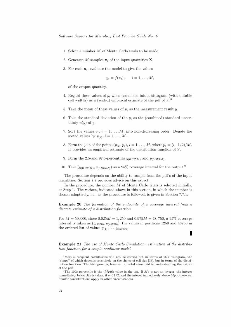
Software Support for Metrology Best Practice Guide No. 6
1. Select a number M of Monte Carlo trials to be made.
2. Generate M samples xi of the input quantities X.
3. For each xi, evaluate the model to give the values
yi = f(xi), i = 1, . . . ,M,
of the output quantity.
4. Regard these values of yi when assembled into a histogram (with suitablecell widths) as a (scaled) empirical estimate of the pdf of Y .8
5. Take the mean of these values of yi as the measurement result y.
6. Take the standard deviation of the yi as the (combined) standard uncer-tainty u(y) of y.
7. Sort the values yi, i = 1, . . . ,M , into non-decreasing order. Denote thesorted values by y(i), i = 1, . . . ,M .
8. Form the join of the points (y(i), pi), i = 1, . . . ,M , where pi = (i−1/2)/M .It provides an empirical estimate of the distribution function of Y .
9. Form the 2.5-and 97.5-percentiles y(0.025M) and y(0.975M).
10. Take (y(0.025M), y(0.975M)) as a 95% coverage interval for the output.9
The procedure depends on the ability to sample from the pdf’s of the inputquantities. Section 7.7 provides advice on this aspect.
In the procedure, the number M of Monte Carlo trials is selected initially,at Step 1. The variant, indicated above in this section, in which the number ischosen adaptively, i.e., as the procedure is followed, is given in Section 7.7.1.
Example 20 The formation of the endpoints of a coverage interval from adiscrete estimate of a distribution function
For M = 50, 000, since 0.025M = 1, 250 and 0.975M = 48, 750, a 95% coverageinterval is taken as (y(1250), y(48750)), the values in positions 1250 and 48750 inthe ordered list of values y(1), . . . , y(50000).
Example 21 The use of Monte Carlo Simulation: estimation of the distribu-tion function for a simple nonlinear model
8Most subsequent calculations will not be carried out in terms of this histogram, the“shape” of which depends sensitively on the choice of cell size [33], but in terms of the distri-bution function. The histogram is, however, a useful visual aid to understanding the natureof the pdf.
9The 100p-percentile is the (Mp)th value in the list. If Mp is not an integer, the integerimmediately below Mp is taken, if p < 1/2, and the integer immediately above Mp, otherwise.Similar considerations apply in other circumstances.
62

Uncertainty and Statistical Modelling
0 1 2 3 4 5 6 7 80
0.1
0.2
0.3
0.4
0.5
0.6
0.7
0.8
0.9
1
Figure 7.1: An empirical estimate obtained using Monte Carlo Simulation, with500 trials, of the distribution function for the model Y = X2
1 . X1 has a proba-bility density function that is Gaussian with mean 1.2 and standard deviation0.5.
0 1 2 3 4 5 6 7 80
5
10
15
20
25
Figure 7.2: A histogram of the values used to produce the distribution functionof Figure 7.1. It constitutes a discrete, scaled representation of the correspond-ing probability density function.
Consider the univariate model Y = X21 , where the single input X1 has a Gaus-
sian pdf with mean 1.2 and standard deviation 0.5. Determine the pdf anddistribution function of Y , the mean and standard deviation of Y and a 95%coverage interval for the measurand.
First, the number M of Monte Carlo trials was taken as 500. Values xi,i = 1, . . . ,M , were sampled from the Gaussian distribution having mean 1.2and standard deviation 0.5. The corresponding values yi = x2
i , i = 1, . . . ,M ,were calculated according to the model. The empirical distribution function ofY was taken, in accordance with the above, as the join of the points (y(i), pi),i = 1, . . . ,M , where pi = (i−1/2)/M . Figure 7.1 shows the distribution functionso obtained.
A histogram of the values of yi appears as Figure 7.2. It constitutes adiscrete, scaled representation of the pdf.
The empirical distribution function is a much smoother function than theempirical pdf, the main reason for which is that the empirical distribution func-tion constitutes a cumulative sum of the empirical pdf. Taking successive sumsis a smoothing process, being the converse of taking successive differences. Thissummation corresponds to the integration counterpart for analytical pdf’s.
The exercise was repeated for M = 50, 000 trials. See Figures 7.3 and 7.4.
63
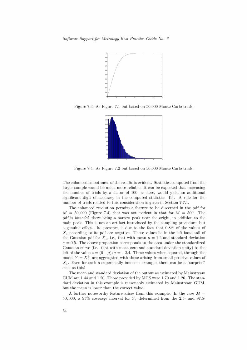
Software Support for Metrology Best Practice Guide No. 6
0 2 4 6 8 10 120
0.1
0.2
0.3
0.4
0.5
0.6
0.7
0.8
0.9
1
Figure 7.3: As Figure 7.1 but based on 50,000 Monte Carlo trials.
0 2 4 6 8 10 120
200
400
600
800
1000
1200
1400
1600
1800
2000
Figure 7.4: As Figure 7.2 but based on 50,000 Monte Carlo trials.
The enhanced smoothness of the results is evident. Statistics computed from thelarger sample would be much more reliable. It can be expected that increasingthe number of trials by a factor of 100, as here, would yield an additionalsignificant digit of accuracy in the computed statistics [19]. A rule for thenumber of trials related to this consideration is given in Section 7.7.1.
The enhanced resolution permits a feature to be discerned in the pdf forM = 50, 000 (Figure 7.4) that was not evident in that for M = 500. Thepdf is bimodal, there being a narrow peak near the origin, in addition to themain peak. This is not an artifact introduced by the sampling procedure, buta genuine effect. Its presence is due to the fact that 0.8% of the values ofX1 according to its pdf are negative. These values lie in the left-hand tail ofthe Gaussian pdf for X1, i.e., that with mean µ = 1.2 and standard deviationσ = 0.5. The above proportion corresponds to the area under the standardizedGaussian curve (i.e., that with mean zero and standard deviation unity) to theleft of the value z = (0−µ)/σ = −2.4. These values when squared, through themodel Y = X2
1 , are aggregated with those arising from small positive values ofX1. Even for such a superficially innocent example, there can be a “surprise”such as this!
The mean and standard deviation of the output as estimated by MainstreamGUM are 1.44 and 1.20. Those provided by MCS were 1.70 and 1.26. The stan-dard deviation in this example is reasonably estimated by Mainstream GUM,but the mean is lower than the correct value.
A further noteworthy feature arises from this example. In the case M =50, 000, a 95% coverage interval for Y , determined from the 2.5- and 97.5-
64

Uncertainty and Statistical Modelling
percentiles of the empirical distribution function was [0.1, 4.8]. That providedusing Mainstream GUM is [−1.1, 3.9] or, equivalently, 1.4 ± 2.5. The lengthsof the coverage interval are similar. However, the interval provided by Main-stream GUM is shifted left relative to that for MCS. In fact, the portion of theMainstream GUM coverage interval from -0.8 to zero is infeasible, since, fromits definition, Y cannot be negative.
Coverage intervals at other levels of probability were also obtained usingMCS and Mainstream GUM. Appreciable differences were again observed. Forinstance, at a 99.8% level of probability (corresponding to a coverage factor of3 under the Gaussian assumption), the coverage interval provided by MCS was[0.0, 7.5] and that for Mainstream GUM is [−2.3, 5.2].
Although the above example might seem extreme, situations with large un-certainties arise in metrology areas such as EMC measurement. Instances wherethe quotient of the standard uncertainty and the mean are of order unity alsoarise, e.g., in dimensional metrology and in photometry and radiometry. Thereare also problems in limits of detection (Section 9.5), where the uncertaintiesinvolved are comparable to the magnitudes of the quantities measured.
The effect of bias in the evaluated endpoints of the coverage interval con-structed in this way, resulting from the use of a finite sample, can be reducedusing so-called bias-corrected methods [30].10
7.3.1 Computation time
An indication of the computation time required for Monte Carlo calculationscan be obtained from the following figures.
A problem with a model consisting of the sum of five terms, a cosine, a sine,an inverse tangent, an exponential and a square root was synthesised. Eachterm was assigned a Gaussian pdf. M = 106 Monte Carlo trials were made.Computation time for a 1 GHz Pentium 3 PC using Matlab are as follows.
The generation of the 5M Gaussian pseudo-random numbers takes 1 s.The evaluation of the M model values takes 1 s.To sort the M estimates of the output into non-decreasing order to produce
the output distribution function takes 3 s.11
Thus, the computation time totals 5 s.This information provides a simple basis for estimating the computation
time for other models, other values of M and other PCs.
7.4 Monte Carlo Simulation for multivariate mod-els
Consider the counterpart of Section 7.2 for multivariate models. The model isnow
Y = f(X).
10In the authors’ experience these corrections typically have a small effect. This aspect,however, merits further study.
11The sorting should be carried out using a sorting algorithm that takes a number of op-erations proportional to M log M [55]. A naive sorting algorithm would take a number ofoperations proportional to M2 that might make the computation time unacceptably long.
65

Software Support for Metrology Best Practice Guide No. 6
M samples xi of the input quantities X are taken as before. For each xi,evaluate the model as previously, except now the values of the output quantitiesare yi = f(xi), m× 1 vectors.
Assemble these vector output quantities into an m×M matrix12:
Υ = (y1, . . . ,yM ).
From this matrix the covariance matrix Vy can be estimated. It is readilyverified that
Vy =1
M − 1Υ′(Υ′)T,
where Υ′ is Υ corrected for the sample means over all M trials, i.e., with themean of the jth row subtracted from all elements in that row, for j = 1, . . . ,M .
This covariance matrix contains (generally a more reliable estimate of) theinformation that would be delivered by a linear analysis such as MainstreamGUM. (In fact, it provides more than Mainstream GUM, since that proceduredoes not in general cover multivariate models.) The matrix Υ provides muchricher information, however, in the following sense. Consider any function ofthe output quantities, i.e., the “next” output quantities in a subsequent stage ofa multi-stage process for which the input quantities are those output quantities.The function evaluated for any column of Υ is an instance of the next outputquantity. Since this output quantity can be calculated for all columns, theresulting 1 × M row vector providing an empirical sampling distribution forthat quantity. In particular, percentiles of the values in that vector can beused, as above, to provide a coverage interval for the derived quantity. Anotherquantity could be so introduced and the two row vectors used to compute anystatistics required (mean, median, etc.) and the pair of vectors used to estimatecorrelation effects. Thus, the matrix Υ is a very valuable array, being the basisof almost unlimited statistical information.
The extension of the approach to the evaluation of coverage regions formultivariate measurement results is not straightforward, because the operationof sorting multivariate data is generally not well-defined. Some approaches havebeen proposed [3], including the ranking of multivariate data using the metric
(yi − a)TΣ−1(yi − a), (7.1)
where a is a location statistic, such as the mean or (spatial) median [58], for theset yi and Σ is a dispersion statistic, such as the covariance matrix Vy, for theset.
The provision of coverage regions in general is currently a research topic.A simple, practical approach is therefore proposed for current purposes. Asindicated in Section 3.1, even in the univariate case the coverage interval is notunique. There is far greater freedom of choice in the multivariate case, whereany domain containing 95% of the distribution of possible values constitutes a95% coverage region. Moreover, a coverage interval can be expressed in termsof just two quantities, such as the interval endpoints or the interval midpointand the semi-width. In more than one dimension, there is an infinite number ofpossibilities for the shape of the region.
12The symbol Υ is (reluctantly) used to denote the matrix of y-vectors, since Y is used todenote a scalar output quantity and Y a vector output quantity.
66

Uncertainty and Statistical Modelling
A working approach is as follows. For linear or linearized problems the co-variance matrix of the (vector) output quantity defines a one-standard-deviationellipsoid [51] centred on the point denoting the estimate of the output quantity.Ellipsoids concentric with this one contain various fractions of the distributionof values attributed to the output quantity. For a given level of probability,95%, say, the size of the ellipsoid from this set can be found (using the theoryof multidimensional Gaussian distributions) that contains 95% of the possiblevalues of the output. Such an ellipsoid can be constructed from the above co-variance matrix, but its size would be dictated by the Gaussian assumptionand not depend on the actual distribution of the values of yi. An ellipsoid isrequired that contains 95% of the actual distribution. In the univariate case, itis more valid, as considered in Section 7.3, to derive the coverage interval fromthe information contained in the empirical estimate of the actual pdf. Similarly,in the multivariate case the points yi define a cluster of points centered on y.These yi can be expected to reflect faithfully the actual distribution, as a con-sequence of the sampling approach used, Therefore, it is recommended to definea coverage region by the (first-order) ellipsoid that (just) contains 95% of theseyi.
It is emphasized that this approach will provide a 95% coverage region. Theextent to which it is appropriate depends on the context. It may be highly in-appropriate if the actual distribution of points yi is, say, star-shaped. However,the approach is consistent with the use of the metric (7.1) with Σ = Vy.
7.5 Extensions to implicit or complex-valued mod-els
The extension of the above concepts to implicit models is conceptually straight-forward. Instead of forming values yi = f(xi) of the output quantity Y in theunivariate case or yi = f(xi) of Y in the multivariate case, by evaluating a for-mula or formulae, it is necessary to solve, respectively, the equation h(yi,xi) = 0for yi or the equations h(yi,xi) = 0 for yi. (See Chapter 6.)
7.6 Disadvantages and advantages of MCS
There are several disadvantages of MCS and a (greater) number of advantages.The attributes of the approach are briefly reviewed.
7.6.1 Disadvantages
1. Availability of pseudo-random number generators. Pseudo-random num-ber generators are required that are appropriate for the specified pdf’s andjoint pdf’s of the input quantities that are likely to arise in metrology.
2. Quality of pseudo-random number generators. Some pseudo-random num-ber generators are known to yield sequences of values that fail to satisfystandard tests for randomness.
3. Repeatability properties. The results may not be repeatable, thus makingthe testing of MCS software harder. The same random number generator,
67
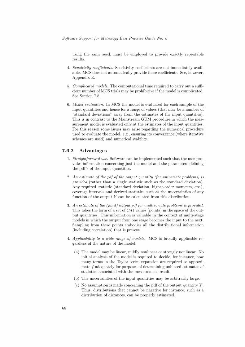
Software Support for Metrology Best Practice Guide No. 6
using the same seed, must be employed to provide exactly repeatableresults.
4. Sensitivity coefficients. Sensitivity coefficients are not immediately avail-able. MCS does not automatically provide these coefficients. See, however,Appendix E.
5. Complicated models. The computational time required to carry out a suffi-cient number of MCS trials may be prohibitive if the model is complicated.See Section 7.8.
6. Model evaluation. In MCS the model is evaluated for each sample of theinput quantities and hence for a range of values (that may be a number of“standard deviations” away from the estimates of the input quantities).This is in contrast to the Mainstream GUM procedure in which the mea-surement model is evaluated only at the estimates of the input quantities.For this reason some issues may arise regarding the numerical procedureused to evaluate the model, e.g., ensuring its convergence (where iterativeschemes are used) and numerical stability.
7.6.2 Advantages
1. Straightforward use. Software can be implemented such that the user pro-vides information concerning just the model and the parameters definingthe pdf’s of the input quantities.
2. An estimate of the pdf of the output quantity (for univariate problems) isprovided (rather than a single statistic such as the standard deviation).Any required statistic (standard deviation, higher-order moments, etc.),coverage intervals and derived statistics such as the uncertainties of anyfunction of the output Y can be calculated from this distribution.
3. An estimate of the (joint) output pdf for multivariate problems is provided.This takes the form of a set of (M) values (points) in the space of the out-put quantities. This information is valuable in the context of multi-stagemodels in which the output from one stage becomes the input to the next.Sampling from these points embodies all the distributional information(including correlation) that is present.
4. Applicability to a wide range of models. MCS is broadly applicable re-gardless of the nature of the model:
(a) The model may be linear, mildly nonlinear or strongly nonlinear. Noinitial analysis of the model is required to decide, for instance, howmany terms in the Taylor-series expansion are required to approxi-mate f adequately for purposes of determining unbiased estimates ofstatistics associated with the measurement result.
(b) The uncertainties of the input quantities may be arbitrarily large.
(c) No assumption is made concerning the pdf of the output quantity Y .Thus, distributions that cannot be negative for instance, such as adistribution of distances, can be properly estimated.
68

Uncertainty and Statistical Modelling
5. Symmetry is not assumed. No assumption is made in using MCS concern-ing the symmetry of the input quantities or the output quantity. Thus,there is no need to “symmetrize” any pdf, or indeed any advantage gainedfrom doing so.13
6. Derivatives are not required. There is no need for algebraic expressions forthe first-order partial derivatives of the model with respect to the inputquantities and for the evaluation of these expressions at the mean valuesof the input quantities.
7. Avoidance of the concept of effective degrees of freedom. MCS avoids theconcept of effective numbers of degrees of freedom: an experimental meanand a standard deviation of a quantity, for which a Gaussian prior has beenassumed, are described by a posterior density, viz., a linearly transformedStudent’s-t distribution with the mean as the location parameter and thestandard deviation as the scale parameter.14
8. Linear computing time. The computing time is dominated by the productof the number of trials and the time to evaluate the model f for a setof input values. Over and above this, it is independent of the numbern of inputs. (This is not the case for the numerical evaluation of themultivariate integral (3.1) that defines Y , where the computation time isessentially proportional to Cn, for some constant C.)
9. Sensitivities can be calculated. MCS does not automatically provide sensi-tivity coefficients, for two reasons. First, they are not required for purposesof its operation. Second, for a nonlinear model, sensitivity coefficients arein general approximate, the quality of the approximations worsening withincreased standard deviations for the input pdf’s. However, simply byholding all input quantities but one fixed at their mean values MCS canbe used to provide the pdf for the output quantity for the model havingjust that input quantity. See Section E.
10. Multi-stage models. MCS can take the output matrix Υ of vectors yi fromone stage of a multi-stage model, and carry out bootstrap-like re-samplingat the input to the next.
7.7 Implementation considerations
This section is concerned with two implementation aspects of MCS, (i) samplingfrom the pdf’s of the input quantities and (ii) carrying out an appropriatenumber of Monte Carlo trials.
13The (UK) Royal Society of Chemistry state [17] that “Such an assumption [the use ofa single parameter–often taken to be the half-range] is appropriate only if the “dispersion ofvalues” is nearly symmetric about the measured result. It is easy to think of reasons why thismay be false, including the effects of contamination and of range shifting on instruments”.
14A discussion [36] of this issue suggests that in the case of a finite number of degrees offreedom the standard deviation u of the Gaussian distribution should also be regarded as arandom variable. In this regard, a pdf should also be attached to u. Because of the Gaussianassumption this pdf is distributed as χ2. A pseudo-code is available [36] that accounts forthis effect.
69

Software Support for Metrology Best Practice Guide No. 6
Probability density functions that are commonly assigned to the input quan-tities are the uniform, the Gaussian, the Student’s-t, and the multivariate Gaus-sian. Methods, in the form of pseudo-random number generators, for samplingfrom these pdf’s are available in a companion document [20].
Other pdf’s arise from time to time: Binomial, Gamma (including Exponen-tial and χ2, Beta, Poisson, truncated Gaussian, etc.). The next edition of thisdocument will cover such pdf’s. Moreover, a general approach that is applicableto any pdf will be outlined.
Knowing when to stop the MCS process is discussed below. This aspect isimportant in terms of (a) carrying out an adequate number of trials in orderthat the process has “converged” according to a specified threshold, and (b) notcarrying an excessive and hence uneconomic number of trials.
7.7.1 Knowing when to stop
When applying MCS the quality of the results depends on the number of MCStrials made. It is not possible to say a priori how many trials will be requiredto achieve a prescribed accuracy in the results. The reason is that the numberwill depend on the “shape” of the pdf and the level of probability required.Also, the calculations are stochastic in nature, being based on random sam-pling. Therefore, any discussion concerning “convergence” cannot be couchedin the traditional numerical analysis setting of iterative methods for determin-istic problems.
Here, a recommendation is made for determining the number of trials neededto provide a coverage interval at, for definiteness, a 95% level of probability towithin a stipulated accuracy. It is necessary to define what is meant by accuracy.The following definition accords with the general sentiments of the GUM inreporting uncertainty. It is also consistent with earlier advice [10]. Supposethat two correct figures15 are required in the standard deviation u(y) of themeasurement result y. The actual value of u(y) will have a certain numberq, say, of digits after the decimal point given by rounding that value to twosignificant decimal figures.
Example 22 The number of digits after the decimal point in rounding a stan-dard uncertainty
Suppose the measurement result for a nominally 100 g standard of mass [1,Clause 7.2.2] is y = 100.021 47 g and the standard uncertainty of y, rounded totwo significant figures, is u(y) = 0.000 35 g, The number of digits in u(y) afterthe decimal point is q = 5.
A coverage interval whose endpoints are known to a specified accuracy (viz.,q correct digits after the decimal point) is sought. However, because the sam-pling process is stochastic, no guarantee can be given that the required accuracyhas been achieved. Instead the practical goal of determining the endpoints ofthe coverage interval to meet a statistical criterion is set. Within the contextof the sampling process, it is possible to state a 95% coverage interval for theendpoints of a computed coverage interval.
15The approach is easily modified for other numbers of correct figures. Two figures (or oftenone figure) are nearly always adequate.
70

Uncertainty and Statistical Modelling
It was stated in Section 7.3 that after M MCS trials, the endpoints of acoverage interval for Y are the 2.5-and 97.5-percentiles y(0.025M) and y(0.975M).The endpoints of a coverage interval for the (100p)th percentile are [6] Mp ±2Mp(1−p)1/2. For the 2.5- and 97.5-percentiles, these endpoints are 0.025M±0.31M1/2 and 0.975M ± 0.31M1/2. Let
L− = [0.025M − 0.31M1/2],L = [0.025M ],
L+ = [0.025M + 0.31M1/2],H− = [0.975M − 0.31M1/2],H = [0.975M ],
H+ = [0.975M + 0.31M1/2].
M is large enough when the lengths y(L+)−y(L−) and y(H+)−y(H−) of the 95%coverage intervals for the endpoints y(L) and y(H) are no larger than 0.5×10−q,
A practical and easily implemented approach consists of carrying out M =5, 000 (say) trials initially, calculating the value of u(y) from these results, form-ing the value of q, computing the coverage interval and carrying out the aboveaccuracy check. If the check was satisfied, accept the result. Otherwise, carryout a further 5000 trials, and recompute u(y), q and the coverage interval basedon the aggregated (increased) number of trials and carry out the checks again.Repeat the process as many times as necessary.16
Example 23 An appropriate number of Monte Carlo trials to be taken whendetermining the measurement uncertainty of a hand-held multimeter
Consider the example of Section 9.3 concerned with the calibration of a hand-held multimeter. Table 7.1 shows the application of the above procedure. Thefirst column in the table gives the total number of trials taken. The secondcolumn gives the number of digits after the decimal point in the value of u(y),the standard deviation of the M values yi of the measurand Y ≡ EX determinedso far. The third column contains the value of u(y). The columns headed y(L)
and y(H) give the endpoints of the coverage interval formed from the appropriatepercentiles of the yi. The columns headed y(L−) and y(L+) give the lower andupper endpoints of the coverage interval for y(L), and y(H−) and y(H+) similarlyfor y(H). The columns headed L-len and H-len give the lengths of these endpointcoverage intervals.
It is seen that these lengths reduce approximately as M−1/2, in accordancewith the point made in Section 7 concerning convergence.17 60,000 trials wereneeded to reduce both of these lengths to 0.0005, and thus to give a good degreeof assurance that the coverage interval for Y ≡ EX was computed correctly tothree figures after the decimal point, in accordance with providing two significantfigures in u(y). The resulting coverage interval for the measurand, defined by
16Because the value of u(y) is much better defined by a relatively small number of trialsthan are the endpoints of a coverage interval, subsequent values of u(y) are unlikely to changemuch from their original values. In contrast, the coverage interval will take longer to settledown.
17For instance, when M is increased from 15 000 to 60 000, i.e., increased by a factor offour, L-len and H-len are approximately halved, reducing from 0.0009 to 0.0005 and from0.0010 to 0.0005, respectively.
71
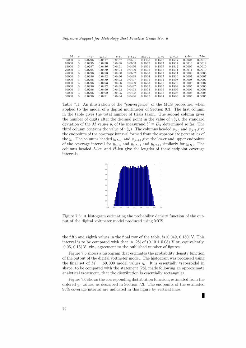
Software Support for Metrology Best Practice Guide No. 6
M q u(y) y(L−) y(L) y(L+) y(H−) y(H) y(H+) L-len H-len5000 3 0.0296 0.0477 0.0487 0.0501 0.1498 0.1508 0.1517 0.0024 0.0019
10000 3 0.0295 0.0490 0.0495 0.0503 0.1502 0.1507 0.1514 0.0013 0.001215000 3 0.0297 0.0486 0.0491 0.0496 0.1501 0.1507 0.1512 0.0009 0.001020000 3 0.0295 0.0489 0.0494 0.0499 0.1501 0.1506 0.1511 0.0011 0.001025000 3 0.0296 0.0493 0.0498 0.0502 0.1503 0.1507 0.1511 0.0009 0.000830000 3 0.0296 0.0492 0.0496 0.0499 0.1504 0.1507 0.1510 0.0007 0.000735000 3 0.0296 0.0489 0.0493 0.0497 0.1501 0.1504 0.1508 0.0008 0.000740000 3 0.0296 0.0493 0.0496 0.0499 0.1503 0.1506 0.1510 0.0006 0.000745000 3 0.0296 0.0492 0.0495 0.0497 0.1502 0.1505 0.1508 0.0005 0.000650000 3 0.0296 0.0490 0.0493 0.0495 0.1503 0.1506 0.1509 0.0006 0.000655000 3 0.0296 0.0492 0.0495 0.0498 0.1503 0.1505 0.1508 0.0005 0.000560000 3 0.0296 0.0491 0.0494 0.0496 0.1502 0.1504 0.1506 0.0005 0.0005
Table 7.1: An illustration of the “convergence” of the MCS procedure, whenapplied to the model of a digital multimeter of Section 9.3. The first columnin the table gives the total number of trials taken. The second column givesthe number of digits after the decimal point in the value of u(y), the standarddeviation of the M values yi of the measurand Y ≡ EX determined so far. Thethird column contains the value of u(y). The columns headed y(L) and y(H) givethe endpoints of the coverage interval formed from the appropriate percentiles ofthe yi. The columns headed y(L−) and y(L+) give the lower and upper endpointsof the coverage interval for y(L), and y(H−) and y(H+) similarly for y(H). Thecolumns headed L-len and H-len give the lengths of these endpoint coverageintervals.
0.02 0.04 0.06 0.08 0.1 0.12 0.14 0.16 0.180
200
400
600
800
1000
1200
1400
1600
Figure 7.5: A histogram estimating the probability density function of the out-put of the digital voltmeter model produced using MCS.
the fifth and eighth values in the final row of the table, is [0.049, 0.150] V. Thisinterval is to be compared with that in [28] of (0.10± 0.05) V or, equivalently,[0.05, 0.15] V, viz., agreement to the published number of figures.
Figure 7.5 shows a histogram that estimates the probability density functionof the output of the digital voltmeter model. The histogram was produced usingthe final set of M = 60, 000 model values yi. It is essentially trapezoidal inshape, to be compared with the statement [28], made following an approximateanalytical treatment, that the distribution is essentially rectangular.
Figure 7.6 shows the corresponding distribution function, estimated from theordered yi values, as described in Section 7.3. The endpoints of the estimated95% coverage interval are indicated in this figure by vertical lines.
72
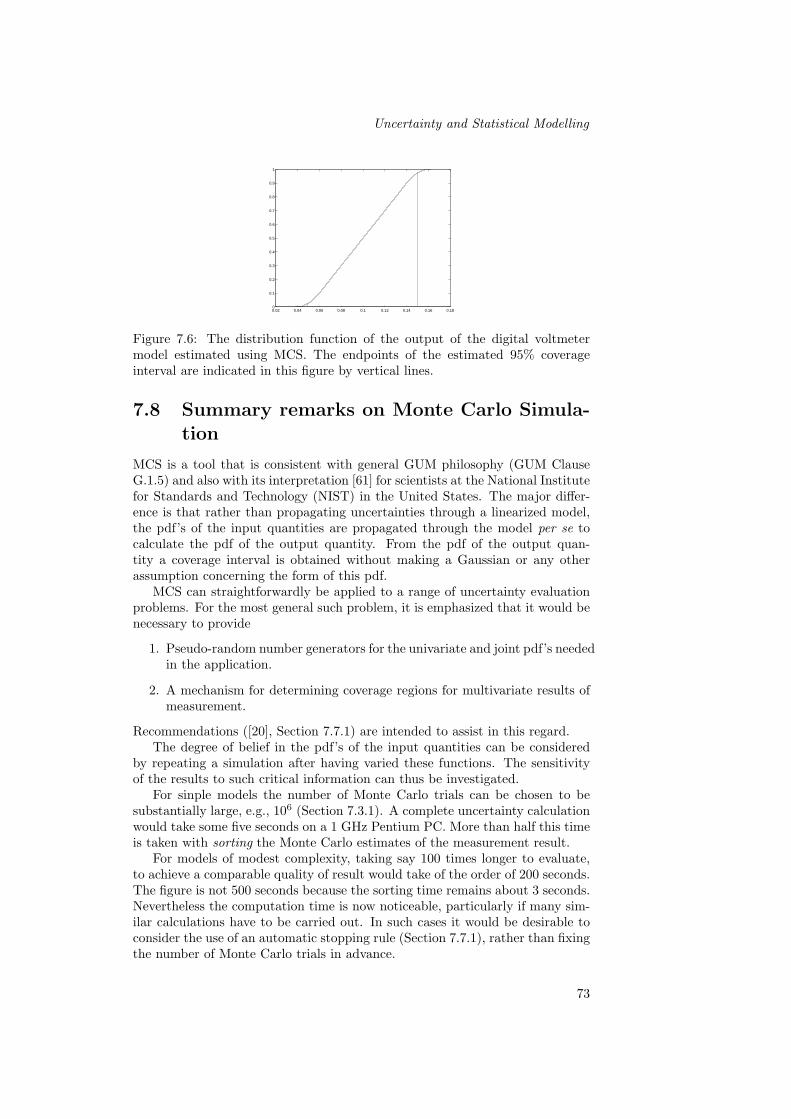
Uncertainty and Statistical Modelling
0.02 0.04 0.06 0.08 0.1 0.12 0.14 0.16 0.180
0.1
0.2
0.3
0.4
0.5
0.6
0.7
0.8
0.9
1
Figure 7.6: The distribution function of the output of the digital voltmetermodel estimated using MCS. The endpoints of the estimated 95% coverageinterval are indicated in this figure by vertical lines.
7.8 Summary remarks on Monte Carlo Simula-tion
MCS is a tool that is consistent with general GUM philosophy (GUM ClauseG.1.5) and also with its interpretation [61] for scientists at the National Institutefor Standards and Technology (NIST) in the United States. The major differ-ence is that rather than propagating uncertainties through a linearized model,the pdf’s of the input quantities are propagated through the model per se tocalculate the pdf of the output quantity. From the pdf of the output quan-tity a coverage interval is obtained without making a Gaussian or any otherassumption concerning the form of this pdf.
MCS can straightforwardly be applied to a range of uncertainty evaluationproblems. For the most general such problem, it is emphasized that it would benecessary to provide
1. Pseudo-random number generators for the univariate and joint pdf’s neededin the application.
2. A mechanism for determining coverage regions for multivariate results ofmeasurement.
Recommendations ([20], Section 7.7.1) are intended to assist in this regard.The degree of belief in the pdf’s of the input quantities can be considered
by repeating a simulation after having varied these functions. The sensitivityof the results to such critical information can thus be investigated.
For sinple models the number of Monte Carlo trials can be chosen to besubstantially large, e.g., 106 (Section 7.3.1). A complete uncertainty calculationwould take some five seconds on a 1 GHz Pentium PC. More than half this timeis taken with sorting the Monte Carlo estimates of the measurement result.
For models of modest complexity, taking say 100 times longer to evaluate,to achieve a comparable quality of result would take of the order of 200 seconds.The figure is not 500 seconds because the sorting time remains about 3 seconds.Nevertheless the computation time is now noticeable, particularly if many sim-ilar calculations have to be carried out. In such cases it would be desirable toconsider the use of an automatic stopping rule (Section 7.7.1), rather than fixingthe number of Monte Carlo trials in advance.
73

Software Support for Metrology Best Practice Guide No. 6
For very complicated models18 it would not be economic to take more than asmall number of trials (say 10). In such a case it would be impossible to providea coverage interval reliably. Rather, a mean and standard deviation should beobtained and a coverage interval obtained assuming a Gaussian distribution.(Appeal can be made to the Principle of Maximum Entropy.) For multivariateoutput quantities a covariance matrix from the results can be calculated anda multivariate Gaussian distribution assumed. As always, the results obtainedshould be accompanied by a statement that indicates clearly how they wereobtained.
18An instance is a model defined by a partial differential equation.
74
Uncertainty and Statistical Modelling
Chapter 8
Validation of MainstreamGUM
This chapter describes validation tests that can be carried out to decide whetherMainstream GUM is applicable in any particular circumstance. There are twotypes of test, prior tests and post tests, carried out, respectively, before utilizingMainstream GUM and after having applied Mainstream GUM.
The post-test involves the use of MCS as the validation tool.
8.1 Prior test: a quick test of whether modellinearization is valid
Mainstream GUM uses the first-order Taylor expansion of the model as part ofevaluating the uncertainty associated with the result of measurement.
A quick test is described that can be used to help decide whether the first-order Taylor series approximation employed by Mainstream GUM is adequate.The test applies to a model with uncorrelated input quantities. Using the no-tation of Section 6.2.1, consider the standard uncertainty u(y) in the outputquantity y obtained from
u2(y) =n∑
i=1
c2i u
2(xi),
a formula obtained from (6.2) when all covariances are set to zero, and ci denotes∂f/∂Xi evaluated at X = x. The test is based on generating, for each modelinput Xi, not just a single value of the sensitivity coefficient ci but three valuesthat are realistically likely to encompass the range of values of the first-orderpartial derivative for that input quantity in the neighbourhood of its estimatedvalue. If the variation in these values is small enough, for all input quantities,a first-order evaluation is adequate. “Small enough” means that the variationis no greater than the required numerical accuracy of the solution uncertainty.“In the neighbourhood” means, for each i, the interval about xi that covers,say, 95% of the distribution of values of the input quantity. Thus, if one correctfigure in a relative sense is sought, this relative variation is not to exceed 0.05.Compare with Section 7.7.1.
75

Software Support for Metrology Best Practice Guide No. 6
This test is severe. If just one of the model input quantities failed the test,the test overall would be regarded as failing, which would be unreasonable ifthat quantity made a negligible contribution to u(y).
A less extreme and more practical test is (i) to evaluate u(y) for the smallestof the three sensitivity coefficients for each component, (ii) as (i) but for thelargest sensitivity coefficient, and (iii) to test whether the two estimates of u(y)agreed to one figure.
For each value of i from 1 to n, take the variation over the range x(low)i
to x(high)i , the 2.5- and 97.5-percentiles of the pdf of xi.1 The rationale for
this choice is that the pdf of y is likely to be dominated by contributions fromthe input pdf’s that are “sufficiently central” to these pdf’s: taking the statedvalues reflects this consideration. The variation of ci regarded as a function ofXi, i.e., ci = ci(Xi), is thus considered over the interval xi±kiu(xi), where ki isthe coverage factor such that 95% of the pdf is embraced.2 It is therefore givenby the interval [cmin
i , cmaxi ], where
cmini = min ci(Xi), cmax
i = max ci(Xi),
where the minimum and maximum are taken over
Xi ∈ [xi − kiu(xi), xi + kiu(xi)].
It is considered unnecessary to determine the actual minimum and maximumvalues in this interval. In the great bulk of cases ci(Xi) would change monoton-ically over the interval, in which case the values at the endpoints would deliverthe required values. If the interval contains an extreme value strictly within it,it is more reliable to take
cmini = minCi, cmax
i = maxCi,
where Ci denotes the set of three values
ci(xi − kiu(xi)), ci(xi), ci(xi + kiu(xi)).
This variant is the one recommended3, particularly because the third pieceof information, ci(xi), would have been evaluated in any case as part of theconventional evaluation of u(y).
The principle can be implemented in the following way.
1. For each value i = 1, . . . , n
1For an input quantity Xi with a Gaussian pdf, xi± 1.96u(xi) can be taken. For an inputquantity Xi with a uniform pdf, take xi ± 1.65u(xi). The multiplier 1.65 is such that 95% ofthe uniform pdf is covered. In general, take the appropriate 95% coverage interval.
2This interval applies to a symmetric pdf. If the pdf is asymmetric the interval becomes
[xi − k(−)i u(xi), xi + k
(+)i u(xi)], where k
(−)i and k
(+)i are factors such that the interval is a
95% coverage interval for Xi. The modifications to be made to the subsequent considerationsare straightforward.
3It is possible to carry out more sophisticated calculations. One approach is to pass aquadratic polynomial through the three sensitivity values, and take its minimum or maximumas appropriate, if such a value lies within the interval. Another possibility is to evaluate ci(Xi)on a fine mesh of values in the interval in order to determine extreme values. Such strategiescould be adopted, but their use would be inconsistent with the intent of the “quick test” ofthis section.
76

Uncertainty and Statistical Modelling
(a) Set ki such that [xi−kiu(xi), xi +kiu(xi)] is a 95% coverage intervalfor Xi.
(b) Form c(mid)i = ∂f(X)/∂Xi, evaluated at x.
(c) Replace the ith component of x by x(low)i = xi − kiu(xi).
(d) Form ci(low) = ∂f(X)/∂Xi, evaluated at x.
(e) Replace the ith component of x by x(high)i . = xi + kiu(xi).
(f) Form c(high)i = ∂f(X)/∂Xi, evaluated at x.
(g) Restore the original value of x.
(h) Form c(min)i = min(c(low)
i , c(mid)i , c
(high)i ).
(i) Form c(max)i = max(c(low)
i , c(mid)i , c
(high)i ).
2. Form u(min)(y) and u(max)(y) from(u(min)(y)
)2
=n∑
i=1
(c(min)i
)2
u2(xi)
and (u(max)(y)
)2
=n∑
i=1
(c(max)i
)2
u2(xi).
3. The prior test is satisfied if
u(y)− u(min)(y) ≤ 0.05u(y)
andu(max)(y)− u(y) ≤ 0.05u(y).
If two correct figures are required, the value of 0.05 in the above procedure isto be replaced by 0.005.
8.2 Validation of Mainstream GUM using MCS
Any case of doubt in the applicability of Mainstream GUM should be validated.In an instance where the Mainstream GUM approach was indeed validated, prac-titioners could safely continue to employ it in that circumstance or in situationsthat could be regarded as comparable. If it was not so validated, it would benecessary to use an alternative procedure in future. It is recommended that theprocess (MCS) at the core of the validation procedure is used for that purpose.
It is essential to note that even if Mainstream GUM had been validated interms of the coverage interval at a specific level of probability, it does not followthat the validation extends to coverage intervals at other levels of probability.For instance, many pdf’s differ in the manner in which their “tails” behave.Thus, good agreement in the 95% coverage intervals that have been providedby Mainstream GUM and MCS by no means applies to, say a 99% level. Thispoint is reinforced by the fact that the graphs of a number of pdf’s tend to“intersect” not far from the endpoints of a 95% coverage interval.
A validation procedure can be based on the following points.
77

Software Support for Metrology Best Practice Guide No. 6
1. Given: Mainstream GUM results in the form of
(a) a measurement result y,
(b) a combined standard uncertainty u(y),
(c) a 95% coverage interval y±U , where U denotes expanded uncertaintydetermined as part of the Mainstream GUM procedure.
2. Given: MCS results in the form of
(a) a measurement result y(MCS),
(b) a corresponding standard uncertainty u(y(MCS)),
(c) the endpoints y(MCS)low and y
(MCS)high of a 95% coverage interval for
the measurand.
3. Define q to be the number of figures after the decimal point in u(y(MCS)),after this value has been rounded to two, say, significant decimal digits.
4. Aim: determine whether there are q correct digits after the decimal pointin u(y) and the endpoints y − U and y + U .
5. Approach: compare the Mainstream GUM and MCS results to determinewhether the required number of correct digits has been obtained.
Further details are available [20].
78

Uncertainty and Statistical Modelling
Chapter 9
Examples
The examples in this chapter are intended to illustrate the principles containedin the body of this guide. Where appropriate, two approaches, MainstreamGUM and Monte Carlo Simulation, are used and contrasted. Some examplescan be regarded as typical of those that arise in metrology. Others are moreextreme, in an attempt to indicate the considerations that are necessary whenthose of “normal circumstances” fail to apply. Perhaps, unfortunately, suchadverse circumstances arise more frequently than would be wished, in areas suchas limit of detection, electromagnetic compliance, photometry and dimensionalmetrology.
Many other examples are given throughout this guide, some to illustratebasic points and others more comprehensive.
9.1 Flow in a channel
This example was provided by the National Engineering Laboratory. It concernsan implicit model arising in channel flow.
Open channel flows are common in the water and hydroelectric power indus-tries and where river extraction provides cooling water for industrial processes.Such a flow can be measured by introducing a specially constructed restrictionin the flow channel. The flow is then a function of the geometry of the restric-tion (width upstream, throat width and length, height of the hump in the floorof the restriction) and the depth of water passing through the restriction.
The model input quantities and estimates of their values are:Approach channel width B = 2.0 m, Throat width b = 1.0 m,Hump height p = 0.25 m, Throat length L = 3.0 m,Nominal head h = 1.0 m
The output quantity is the flow rate Q. The model relating Q to the inputquantities is
Q = (2/3)3/2g1/2CvCDbh3/2,
with g = 9.812 ms−2, the acceleration due to gravity,
CD = (1− 0.006L/b)(1− 0.003L/h)3/2 (9.1)
and4b2h2C2
v − 27B2(h + p)2(C2/3v − 1) = 0. (9.2)
79

Software Support for Metrology Best Practice Guide No. 6
To calculate Q for any values of the input quantities, it is first necessary to formCD from the explicit formula (9.1) and Cv from the implicit equation (9.2).1
The first four input quantities are geometric dimensions obtained by a se-ries of measurements with a steel rule at various locations across the flume.There are uncertainties in these measurements due to location, rule readingerrors and rule calibration. Head height is measured with an ultrasonic detec-tor, uncertainties arising from fluctuations in the water surface and instrumentcalibration.
All uncertainty sources were quantified and appropriate pdf’s assigned. Allpdf’s were based on Gaussian or uniform distributions. The standard deviationsof these pdf’s (standard uncertainties of the input quantities) were all less than0.3% relative to the means (estimated values).
Both the Mainstream GUM procedure (Section 6) and the Monte Carlo pro-cedure (Section 7) were applied. The Mainstream GUM results were validated(Section 8) using the Monte Carlo procedure, under the requirement that resultsto two significant figures were required. In fact, the coverage interval for y asproduced by Mainstream GUM was confirmed correct (by carrying out furtherMonte Carlo trials) to three significant figures. To quote the comparison in arelative sense, the quotient of (a) the half-length of the 95% coverage intervalfor y (≡ Q) and (b) the standard uncertainty of y was 1.96, which agrees tothree significant figures with the Mainstream GUM value, viz., the (Gaussian)coverage factor for 95% coverage. For further comparison, the correspondingquotients corresponding to 92.5% and 97.5% coverage intervals were 1.78 and2.24, also in three-figure agreement with Mainstream GUM results. It is con-cluded that the use of Mainstream GUM is validated for this example for thecoverage probabilities indicated.
9.2 Graded resistors
This example is intended to cover an instance where it would be important totake specific account of the pdf of an input quantity to help ensure that validresults are obtained from an uncertainty evaluation.
The uncertainties of a mass-produced electrical circuit are to be evaluated.The circuit contains electrical components of various types. One of these com-ponent types, a resistor, is considered here.
High-grade (nominally) 1 Ω resistors are graded according to their specifica-tion. A-grade resistors are those that lie within 1% of nominal, B-grade within5% and C-grade within 10%. The allocation of resistors to the various gradesis decided by measurement. For the purposes of this example, the uncertaintyof this measurement is taken as negligible. As each resistor is measured it isallocated to an A-grade, a B-grade, a C-grade or an unclassified “bin”. The al-location is made in the following sequential manner. If a resistor has resistancein the interval (1.00± 0.01) Ω it is allocated to the A-grade bin. If not, and ithas resistance in the interval (1.00± 0.05) Ω it is allocated to the B-grade bin.
1This equation is in fact a cubic equation in the variable C2/3v and, as a consequence, Cv
can be expressed explicitly in terms of B, h and p. Doing so is unwise because of the possiblenumerical instability due to subtractive cancellation in the resulting form. Rather, the cubicequation can be solved using a recognised stable numerical method.
80

Uncertainty and Statistical Modelling
0.9 0.95 1 1.05 1.1 1.150
500
1000
1500
2000
2500
3000
3500
4000
4500
Figure 9.1: A histogram produced by MCS to estimate the probability densityfunction for the Grade-C resistor.
If not, and it has resistance in the interval (1.00± 0.10) Ω it is allocated to theC-grade bin. Otherwise, it is allocated to the unclassified bin.
For the circuit application, C-grade resistors are selected. All such resistorshave a resistance in the interval [0.90, 0.95] Ω or the interval [1.05, 1.10] Ω.From the knowledge of the manufacturing process, the pdf of the resistance ofa resistor before the allocation process is carried out can be taken as Gaussianwith mean 1.00 Ω and standard deviation 0.04 Ω.
Consider the use of three such resistors in series within the circuit to form a(nominally) 3 Ω resistance.
The model for the 3 Ω resistance R is
R = R1 + R2 + R3,
where Ri denotes the resistance of resistor i. Each Ri has a pdf as above. Whatis the pdf of R and what is a 95% coverage interval for R?
Figures are used to show diagrammatically histograms and distribution func-tions of the results of using MCS to estimate the pdf’s. An analytic or semi-analytic treatment is possible, but MCS enables results to be provided rapidly.All results are based on the use of M = 105 Monte Carlo trials.
Figure 9.1 shows a histogram of the pdf of Ri. It is basically Gaussian, withthe central and tail regions removed as a consequence of the grading process.
Figure 9.2 shows the corresponding distribution function produced by MCSin the manner of Section 7.3 The endpoints of the estimated 95% coverageinterval are indicated by vertical dashed lines and the corresponding endpointsunder the Gaussian assumption by vertical dotted lines.
Figure 9.3 shows a histogram produced by MCS to estimate the probabilitydensity function for R, three Grade-C resistors in series.
The pdf is multimodal, possessing four maxima. The mean of the pdf is3.00 Ω, the sum of the means of the three individual pdf’s, as expected. Thisvalue is, however, unrepresentative, an “expectation” that could rarely occur.
Figure 9.4 shows the corresponding distribution function produced in themanner of Section 7.3.
The pdf of Figure 9.3 could be perceived as an overall bell-shape, with strongstructure within it. Indeed, the counterpart of these results for six resistors inseries, as illustrated in Figures 9.5 and 9.6, lies even more in that direction.
Table 9.1 summarises the numerical results, and also includes the resultsfor n = 10 and 20 resistors. It is reassuring that, considering the appreciable
81

Software Support for Metrology Best Practice Guide No. 6
0.85 0.9 0.95 1 1.05 1.1 1.15 1.20
0.1
0.2
0.3
0.4
0.5
0.6
0.7
0.8
0.9
1
0.85 0.9 0.95 1 1.05 1.1 1.15 1.20
0.1
0.2
0.3
0.4
0.5
0.6
0.7
0.8
0.9
1
Figure 9.2: The distribution function corresponding to the probability distri-bution function of Figure 9.1. The endpoints of the estimated 95% coverageinterval are indicated by vertical dashed lines and the corresponding endpointsunder the Gaussian assumption by vertical dotted lines.
2.7 2.8 2.9 3 3.1 3.2 3.3 3.40
500
1000
1500
2000
2500
3000
3500
4000
4500
Figure 9.3: A histogram produced by Monte Carlo Simulation to estimate theprobability density function for R, three Grade-C resistors in series.
0.85 0.9 0.95 1 1.05 1.1 1.15 1.20
0.1
0.2
0.3
0.4
0.5
0.6
0.7
0.8
0.9
1
2.7 2.8 2.9 3 3.1 3.2 3.3 3.40
0.1
0.2
0.3
0.4
0.5
0.6
0.7
0.8
0.9
1
Figure 9.4: The distribution function corresponding to the probability distri-bution function of Figure 9.3. The endpoints of the estimated 95% coverageinterval are indicated by vertical dashed lines and the corresponding endpointsunder the Gaussian assumption by vertical dotted lines.
82

Uncertainty and Statistical Modelling
5.4 5.6 5.8 6 6.2 6.4 6.6 6.80
500
1000
1500
2000
2500
3000
3500
4000
4500
Figure 9.5: A histogram produced by Monte Carlo Simulation to estimate theprobability density function for six Grade-C resistors in series.
0.85 0.9 0.95 1 1.05 1.1 1.15 1.20
0.1
0.2
0.3
0.4
0.5
0.6
0.7
0.8
0.9
1
5.4 5.6 5.8 6 6.2 6.4 6.6 6.80
0.1
0.2
0.3
0.4
0.5
0.6
0.7
0.8
0.9
1
Figure 9.6: The distribution function corresponding to the probability distri-bution function of Figure 9.5. The endpoints of the estimated 95% coverageinterval re indicated by vertical dashed lines and the corresponding endpointsunder the Gaussian assumption by vertical dotted lines.
83
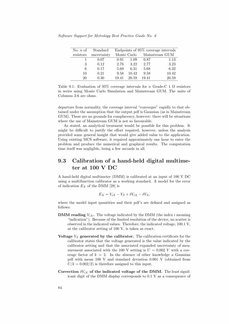
Software Support for Metrology Best Practice Guide No. 6
No. n of Standard Endpoints of 95% coverage intervalsresistors uncertainty Monte Carlo Mainstream GUM
1 0.07 0.91 1.09 0.87 1.133 0.12 2.78 3.22 2.77 3.236 0.17 5.69 6.31 5.68 6.32
10 0.21 9.58 10.42 9.58 10.4220 0.30 19.41 20.59 19.41 20.59
Table 9.1: Evaluation of 95% coverage intervals for n Grade-C 1 Ω resistorsin series using Monte Carlo Simulation and Mainstream GUM. The units ofColumns 2-6 are ohms.
departure from normality, the coverage interval “converges” rapidly to that ob-tained under the assumption that the output pdf is Gaussian (as in MainstreamGUM). These are no grounds for complacency, however: there will be situationswhere the use of Mainstream GUM is not so favourable.
As stated, an analytical treatment would be possible for this problem. Itmight be difficult to justify the effort required, however, unless the analysisprovided some general insight that would give added value to the application.Using existing MCS software, it required approximately one hour to enter theproblem and produce the numerical and graphical results. The computationtime itself was negligible, being a few seconds in all.
9.3 Calibration of a hand-held digital multime-ter at 100 V DC
A hand-held digital multimeter (DMM) is calibrated at an input of 100 V DCusing a multifunction calibrator as a working standard. A model for the errorof indication EX of the DMM [28] is
EX = ViX − VS + δViX − δVS ,
where the model input quantities and their pdf’s are defined and assigned asfollows:
DMM reading ViX . The voltage indicated by the DMM (the index i meaning“indication”). Because of the limited resolution of the device, no scatter isobserved in the indicated values. Therefore, the indicated voltage, 100.1 V,at the calibrator setting of 100 V, is taken as exact.
Voltage VS generated by the calibrator. The calibration certificate for thecalibrator states that the voltage generated is the value indicated by thecalibrator setting and that the associated expanded uncertainty of mea-surement associated with the 100 V setting is U = 0.002 V with a cov-erage factor of k = 2. In the absence of other knowledge a Gaussianpdf with mean 100 V and standard deviation 0.001 V (obtained fromU/k = 0.002/2) is therefore assigned to this input.
Correction δViX of the indicated voltage of the DMM. The least signif-icant digit of the DMM display corresponds to 0.1 V as a consequence of
84

Uncertainty and Statistical Modelling
the finite resolution of the instrument. Each DMM reading is thereforetaken to have a correction of 0.0 V, the error in this value lying in theinterval ±0.05 V . In the absence of other knowledge, a uniform pdf withmean 0.0 V and standard deviation 0.029 V (obtained from 0.05/
√3) is
therefore assigned to this input.
Correction δVS of the calibrator voltage. The calibrator voltage is in prin-ciple corrected for a range of effects including drift, mains power deviationsand loading. An analysis [28] gives a correction of 0.0 V and states thatthe error in this value lies in the interval ±0.011 V .2 In the absence ofother knowledge, a uniform pdf with mean 0.0 V and standard deviation0.0064 V (obtained from 0.011/
√3) is therefore assigned to this input.
This model was analyzed using Monte Carlo Simulation. Details are given inSection 7.7.1. The error of indication of the DMM was found to be 0.100 V witha 95% coverage interval of [0.049, 0.150] V. The corresponding result obtained byan approximate analytical treatment [28] was (0.10± 0.05) V, i.e., in agreementto the figures quoted.
9.4 Sides of a right-angled triangle
This example is intended to illustrate the use of statistical modelling, as de-scribed in Section 4.2. It also illustrates the manner in which correlation effectscan sometimes be removed by the introduction of an additional variable, asindicated in Section 4.2.1.
The sides of a right-angled triangle are repeatedly measured with a length-measuring instrument. The measurements contain random and systematic ef-fects. Use all these measurements to determine best estimates of the sides ofthe triangle and evaluate their uncertainties.
Denote the shorter sides of the triangle by A and B and the hypotenuseby H. Let there be nA measurements of A, nB of B and nH of H. Let theith measurement of A be ai, with error ∆ai, and similarly for B and H. Therelationships between the measurements, the “true” values and the errors are
ai = A + ∆ai, i = 1, . . . , nA,bi = B + ∆bi, i = 1, . . . , nB ,hi = H + ∆hi, i = 1, . . . , nH .
According to Pythagoras’ theorem, the sides are physically related by
A2 + B2 = H2. (9.3)
For consistency, the solution values of A, B and H are to satisfy this condition.The errors ∆ai, etc. are statistically related in that the instrumental sys-
tematic effect will manifest itself in all these values. Its “presence” means thatall measurements are correlated. In order to quantify this correlation, it is
2Since this correction is based on a number of effects, it does not seem reasonable (cf.Section 4.3.3 to regard the error as equally likely to take any value in this interval. However,since the effect of this input on the model output is relatively small, and since an intentionis to compare the EA approach with that of Mainstream GUM, M3003 and MCS, the aboveform is taken.
85

Software Support for Metrology Best Practice Guide No. 6
conventionally necessary to know the standard deviation u(∆L) of the instru-mental systematic effect and the repeatability standard deviation urep of themeasurements.
A covariance matrix based on this correlation can then be established3 andthe above equations solved by least squares with an “input covariance matrix”equal to this covariance matrix. Generic details of this approach, Gauss-Markovestimation, are available [22]. Formally, the result is in the form of a GUM model
Y ≡ (A, B)T = f(a1, . . . , anA, b1, . . . , bnB
, h1, . . . , hnH).
The measurements ai, bi and hi are the input quantities (nA + nB + nH innumber) and A and B are the (two) output quantities. The third side, H,the hypotenuse of the triangle, is not included as an output quantity, since itcan be formed from A and B using (9.3). f denotes the model. It cannot,at least conveniently, be written down mathematically, but is defined by thecomputational procedure that implements the least-squares solution process.
Propagation of the input covariance matrix through the model to providethe covariance matrix of (A, B)T can be carried out as discussed in Section6.2. The use of Equation (9.3) as a “next-stage” model (cf. Section 4.2.3),providing the output H in terms of A and B, can then be used to determinethe uncertainty of H. The results can be combined to provide the covariancematrix of (A, B, H)T.
Statistical modelling can be used to provide the required sides and theiruncertainties without having to work with correlated quantities and, in thisinstance, without prior knowledge of the above standard deviations. Regardthis systematic effect as an unknown bias ∆L and write
∆ai = ∆L + δai,
etc., where δai is the random error in ai, etc. The above relationships become
ai = A + ∆L + δai, i = 1, . . . , nA,bi = B + ∆L + δbi, i = 1, . . . , nB ,hi = H + ∆L + δhi, i = 1, . . . , nH .
The errors δai, etc. are uncorrelated, the covariance matrix being diagonal withall entries equal to u2
rep. Best estimates of the sides (and ∆L) are then givenby an ordinary least-squares problem (Gauss estimation). First, it is necessaryto incorporate the condition (9.3) [22]. There are various ways to do so ingeneral, but here it is simplest to use the condition to eliminate a variable. Onepossibility is to replace H by (A2+B2)1/2 or, letting θ denote the angle betweensides A and H, set
A = H cos θ (9.4)
andB = H sin θ. (9.5)
3The covariance matrix, of order nA + nB + nH , can be built from
1. var(ai) = var(bi) = var(hi) = u2rep + u2(∆L),
2. All covariances are equal to u2(∆L).
(The standard uncertainty u(∆L) associated with the instrumental systematic effects may notbe available explicitly from the calibration certificate of the instrument, but should be part ofthe detailed “uncertainty budget” for the calibration.)
86

Uncertainty and Statistical Modelling
The latter choice gives the least-squares formulation
minH,θ,∆L
S =nA∑i=1
(ai −H cos θ −∆L
urep
)2
+nB∑i=1
(bi −H sin θ −∆L
urep
)2
+nH∑i=1
(hi −H −∆L
urep
)2
.
Its solution could be found using the Gauss-Newton algorithm or one of itsvariants [22].4
Many such problems would be solved in this manner. In this particular case,by defining new parameters
v1 = H cos θ + ∆L, v2 = H sin θ + ∆L, v3 = H + ∆L (9.6)
and v = (v1, v2, v3)T, the problem becomes
minv
nA∑i=1
(ai − v1)2 +nB∑i=1
(bi − v2)2 +nH∑i=1
(hi − v2)2.
The problem separates into three trivial independent minimization problems,giving the solution
v1 = a =nA∑i=1
ai/nA,
and similarly v2 = b and v3 = h.The equations (9.6) can then straightforwardly be solved for H, ∆L and
θ, from which A and B are determined from (9.4) and (9.5). The relevantuncertainties and covariance matrices are readily found using the principles ofSection 6.
Since the value of u2rep is common to all terms in the sum, the minimizing
values of H, θ and ∆L do not depend on it. The term may therefore mayreplaced by unity (or any other constant). Thus, the solution can be obtainedwithout knowledge of the random repeatability uncertainty or the systematicinstrumental uncertainty.
The covariance matrix associated with the solution values of H, θ and ∆Lprovides the required output uncertainties.
9.5 Limit of detection
This example is intended to provide a simple illustration of how measurements ofanalyte concentration at the limit of detection can be analysed to furnish a value
4Advantage can be taken as follows of the fact that the problem is linear in two of theunknowns, H and ∆L. Equate to zero the partial derivatives of S, with respect to H, θ and∆L, to give three algebraic equations. Eliminate H and ∆L to give a single nonlinear equationin θ. Solve this equation using a suitable “zero-finder” (cf. Section 6.2.3). Determine H and∆L by substitution.
87

Software Support for Metrology Best Practice Guide No. 6
Gaussian probability distribution
X
95% cov regx
Figure 9.7: The Gaussian probability density function for the input quantityfor the limit of detection problem. The 95% coverage interval that would con-ventionally be obtained for the analyte concentration is indicated.
for the measurand and its uncertainty. It utilizes basic statistical modellingprinciples.
The framework is as given in Section 4.2.2 on constrained uncertainty eval-uation. The GUM model (4.5), repeated here, is
Y = max(X, 0),
where the input quantity X is observed (unconstrained) analyte concentrationand the measurand Y real (constrained) analyte concentration.
X is estimated by x, the arithmetic mean of a number of (unconstrained)observations of analyte concentration. Its standard uncertainty is estimated bythe standard deviation of this value. At or near the limit of detection, some ofthe observations would be expected to take negative values. If the measurementsrelated to an analytical blank [32, Clause F2.3], used subsequently to correctother results, on average as many negative as positive values might be expected.If the analyte was actually present a preponderance of positive over negativevalues would be expected. Numerical values to represent this latter situationare chosen. The treatment is general, however, and can readily be repeatedfor other numerical values, even including a negative value for the mean of theobservations.
Suppose that nothing is known about the observations other than that theycan be regarded as independently and identically distributed. The use of thePrinciple of Maximum Entropy would indicate that the input X can be re-garded as a Gaussian variable with the above mean and standard deviation.For illustrative purposes, take the mean x = 1.0 ppm and the standard devia-tion u(x) = 1.0 ppm.
The pdf of the input quantity5 and the model are thus fully defined.Figure 9.7 illustrates this Gaussian pdf and indicates the 95% coverage in-
terval that would conventionally be obtained for the analyte concentration.For the above numerical values the corresponding pdf is given in Figure 9.8.The area to the left of the origin under the Gaussian pdf with mean x and
standard deviation u(x) is Φ((0− x)/u(x)) (see Section 4.3.1). The fraction of
5Other pdf’s can be entertained. The subsequent treatment might not be as simple as thathere, but can be addressed using Monte Carlo Simulation or other methods as appropriate.
88

Uncertainty and Statistical Modelling
X
95% cov reg
0
Figure 9.8: As Figure 9.7, but for the case in the text where the mean x =1.0 ppm and the standard deviation u(x) = 1.0 ppm.
X0
Modelinput
Figure 9.9: The pdf for the input quantity for the limit of detection problem
the values of Y = max(X, 0) that is zero is equal to this value. For the abovenumerical values, the fraction is Φ(−1.0) = 0.16. So, 16% of the distribution ofvalues that can plausibly be ascribed to the measurand take the value zero.
The pdf for the input quantity is indicated in Figure 9.9. That for the outputquantity is depicted in Figure 9.10. In Figure 9.10 16% of the area under thecurve is concentrated at the origin. Strictly, this feature should be denoted by aDirac delta function (having “infinite height and zero width”). For illustrativepurposes only, the function is depicted as a “tall thin” solid rectangle.
The shortest 95% coverage interval for the measurand therefore has (a) zeroas its left-hand endpoint, and (b) as right-hand endpoint that value of X forwhich Φ((X − x)/u(x)) = 0.95, viz., X = 2.6 ppm. Thus, the required 95%coverage interval is [0.0, 2.6] ppm.6
Figure 9.11 shows the distribution function G(Y ) for Y , with endpoints of the95% coverage interval indicated by vertical lines. G(Y ) “rises instantaneously”at Y = 0 from zero to 0.16 and thereafter behaves as the Gaussian distributionfunction.7
The mean and standard uncertainty of G(Y ) are readily shown to be y =1.1 ppm and u(y) = 0.9 ppm.
By comparison, the Mainstream GUM approach would yield a result as
6A Monte Carlo Simulation confirms this result.7It is apparent from this figure that if a 95% coverage interval with 2.5% of the distribution
in each tail were chosen the interval would be longer, in fact being [0.0, 3.0] ppm. Of course,since more than 5% of the distribution is at Y = 0, the left-hand endpoint remains at zero forany 95% coverage interval.
89

Software Support for Metrology Best Practice Guide No. 6
Y0
Modeloutput
Figure 9.10: The pdf for the output quantity for the limit of detection problem.16% of the area under the curve is concentrated at the origin. Strictly, thisfeature should be denoted by a Dirac delta function (having “infinite height andzero width”). For illustrative purposes the function is depicted as a “tall thin”solid rectangle.
0 1 2 3 4 5 60
0.1
0.2
0.3
0.4
0.5
0.6
0.7
0.8
0.9
1
Figure 9.11: The distribution function for the limit of detection problem. Theright-hand endpoint of the 95% coverage interval is indicated by a vertical line.the left-hand endpoint is at the origin.
90

Uncertainty and Statistical Modelling
follows. Since, in the neighbourhood of the input estimate x = 1.0 ppm, themodel behaves as Y = max(X, 0) = X, Mainstream GUM gives y = 1.0 ppmas a point estimate of the measurand. Moreover, the sensitivity coefficient c is
∂f
∂X= 1,
evaluated at X = 1.0 ppm, viz., c = 1. Thus,
u(y) = |c|u(x) = 1.0 ppm.
It follows that a 95% coverage interval based on Mainstream GUM considera-tions is (1.0± 2.0) ppm or [−1.0, 3.0] ppm, following the use of Formula (6.2).
This interval is longer than the model-based interval [0.0, 2.6] ppm andextends into the infeasible region. As stated earlier in this example, such an in-terval is appropriate for summarising the observations, but not for the physicallyconstrained measurand, the real analyte concentration.
Similar principles can be applied to the measurement of the concentrationsof a number of solution constituents. The analysis would be harder, but readilysupported by the use of MCS.
9.6 Constrained straight line
The determination of suitable calibration lines and curves is a widespread re-quirement in metrology. The parameters of these lines and curves (and of modelsin general) may have to meet stipulated criteria in order that they reflect ap-propriate physical properties. For instance, a temperature in Kelvin cannot benegative.
Consider the length of a gauge block as its temperature is gradually in-creased. Suppose that for each of a sequence of increasing controlled tempera-ture values the length of the block is measured. It is required to estimate thecoefficient of expansion of the metal of which the block is made. The tempera-tures can be assumed to be known accurately and the measured lengths containerror. It is assumed that these errors have a Gaussian pdf.
A least-squares straight-line fit to the data is appropriate. The gradient ofthe line (the rate of change of length with respect to temperature) provides anestimate of the coefficient of expansion.
It can be shown that the gradient has an error that described by the Student’s-t distribution (cf. [1]). This distribution is the pdf of the output quantity andits use permits a coverage interval for the gradient to be obtained.
This process can often be expected to be satisfactory. This statement applieseven though the Student’s-t distribution has infinite tails, implying that theleft-hand tail includes zero and hence that there is a finite probability that thegradient is negative. This matter is of little concern since the tail probability isoften very small indeed.
There are circumstances, however, where this aspect may be a concern,especially in the context of a procedure or computer software that might beused in a wide range of circumstances.
Consider a gauge block made from a material having a very small coefficientof expansion. In this situation the estimated uncertainty in the coefficient of
91

Software Support for Metrology Best Practice Guide No. 6
expansion could be comparable in size to the value of the coefficient itself. Asa consequence, the application of conventional approaches to determining acoverage interval might produce an interval containing zero! Cf. the limit ofdetection example (Section 9.5).
Alternative approaches, including MCS, can be used to avoid this anomaly.Suppose that MCS is used to compute many estimates of the best-fitting straightline and hence of the gradient (expansion coefficient). Each MCS trial involvessampling from the Gaussian pdf associated with the measured lengths, fittinga constrained line to the sampled data given by these lengths corresponding tothe fixed values of the independent variables, and taking its gradient as thecorresponding measurement result. The set of gradients so obtained form thebasis, as in Section 9.5, for a distribution function of the gradient and hence acoverage interval.
The term “constrained line” is used to indicate the fact that for any set ofsampled data a straight line with an intercept parameter and a gradient param-eter must be fitted subject to the condition that the gradient is not negative. Itis straightforward to use conventional fitting procedures for this purpose. First,a straight line is fitted to the data without imposing the condition. If the gra-dient of the line were positive (or zero) the line would automatically satisfy thecondition and would therefore be the required solution. Otherwise, the “best”line that can be fitted that satisfies the constraint would have a zero gradient.Such a line is a constant. This constant is easily found, since the best least-squares fit by a constant is the same problem as finding the arithmetic mean ofthe data.
Thus the sequence of M , say, gradients so obtained will include some zerovalues, the remainder being strictly positive. The estimated distribution func-tion for the gradient Y , as that for the limit of detection problem (Section 9.5),therefore has a jump discontinuity at y = 0, the magnitude of which is theproportion of trials that gave zero gradient, followed by a “smooth” increasethrough increasing gradient values.
A simple Monte Carlo Simulation was carried out. The data used consistedof the points (18, 23), (19, 24), (20, 26), (21, 27), (22, 28), where the first co-ordinated denotes temperature in C and the second length measurement in anormalised variable. Figure 9.12 depicts the five gauge block length measure-ments against temperature (large blobs) and 100 simulations (small blobs) ofthese measurements obtained from sampling from assigned Gaussian pdf’s. Forthe simulation the standard uncertainty of the length measurements was takenas 0.005 and used as the standard deviation of the Gaussian pdf’s.
For some of the synthesised sets of five measurements the gradient of an un-constrained least-squares straight line would be negative, were it not infeasible.
The results from the use of a large number (100,000) of trials gave a distri-bution function for the gradient very similar to that for the limit of detectionproblem (Section 9.5).
9.7 Fourier transform
Consider measurements of a periodic phenomenon. Such measurements arecommonplace in many branches of metrology. Suppose a complete period is
92

Uncertainty and Statistical Modelling
17 18 19 20 21 22 231
1.01
1.02
1.03
1.04
1.05
1.06
Figure 9.12: The five gauge block length measurements against temperature(large blobs) and 100 simulations of these measurements obtained from sam-pling from assigned Gaussian pdf’s. For some of the synthesised sets of fivemeasurements the gradient of an unconstrained least-squares straight line wouldbe negative.
measured in that n values x = (x1, . . . , xn)T are available. These values corre-spond to the uniformly spaced angles θ = (θ1, . . . , θn)T, where θi = 2π(i−1)/n.
A Fourier transform of such data provides information concerning the fre-quency content of the data.
Each Fourier coefficient depends on all (or most of) the values of xi, regardedas the input quantities, and is a linear combination of them.
Suppose that the errors of measurement can be regarded as mutually inde-pendent with standard deviation σ. The covariance matrix for the measurementerrors or, equivalently, for the input quantities xi, is therefore given by
Vx = σ2I, (9.7)
where I is the identity matrix of order n. It is required to evaluate the uncertain-ties in the Fourier transform of this data, i.e., in the coefficients of the Fourierrepresentation of the data. The coefficients constitute the (vector) measurand.
The Fourier representation of the data is
h(θ) = a0 + a1 cos θ + b1 sin θ + · · ·+ ar cos rθ + br sin rθ,
where r = bn/2c. (When n is even, the coefficient br of sin rθ is in fact zero.)Let y = (y1, . . . , y2r+1)T = (a0, a1, b1, . . . , ar, br)T, the output quantities. TheFourier transform y of x is then given implicitly by
x = Ay, (9.8)
where
A =
1 cos θ1 sin θ1 . . . cos rθ1 sin rθ1
1 cos θ2 sin θ2 . . . cos rθ2 sin rθ2
......
......
......
1 cos θn sin θn . . . cos rθn sin rθn
is the matrix of order n of Fourier basis-function values. Formally, the Fouriercoefficients are given in terms of the data using
y = A−1x (9.9)
93

Software Support for Metrology Best Practice Guide No. 6
or, equivalently, from a formula that expresses the ti as linear combinations ofthe xi, where the multipliers are sine and cosine terms. (In practice, t would becomputed from x using the fast Fourier transform (FFT) [8].) The FFT givesfar greater efficiency than would be obtained from the application of general-purpose linear-algebra techniques, and also greater numerical accuracy.8
Denote the covariance matrix of y by Vy. The application of (6.10) to (9.8)gives
Vx = AVyAT.
This result is exact since the output quantity y and the input quantity x arerelated linearly through (9.8), and linearisation introduces no error in this case.Since A is invertible,
Vy = A−1VxA−T.
This expression enables in general the covariance of the Fourier coefficients tobe computed from that of the data. As a consequence of (9.7),
Vy = σ2A−1A−T = σ2(ATA)−1.
Now, using the fact that θ is equiangular and the fundamental properties of thetrigonometric functions, it is straightforward to show that
ATA =n
2diag
2, 1, . . . , 1
,
giving
(ATA)−1 =2n
diag
12 , 1, . . . , 1
.
Consequently,
Vy =2n
σ2diag
12 , 1, . . . , 1
.
This result states that for data errors that are independent with standard un-certainty σ, the errors in the Fourier coefficients are (also) independent, withstandard uncertainty equal to σ scaled by the factor
√2/n, where n is the
number of points (with the exception of the constant term for which the fac-tor is
√1/n). Moreover, each Fourier coefficient is a linear combination of n
raw data values, the multipliers being the products of a constant value andthat of values of cosines and sines (and thus lying between -1 and +1). Conse-quently, if n is large9 regardless of the statistical distributions of the errors inthe data, the errors in the Fourier coefficients can be expected to be very closeto being normally distributed. This result is an immediate consequence of theCentral Limit Theorem when using the Fourier transform to analyse large num-bers of measurements having independent errors. Thus, it is valid to regard theresulting Fourier coefficients as if they were independent Gaussian-distributedmeasurements.
The outputs, the Fourier coefficients, from this process become the inputsto the subsequent stage, viz., the evaluation of the Fourier series h(θ) for anyvalue of θ. Now, since, as shown, the Fourier coefficients are uncorrelated,
u2(h(θ)) = u2(a0)+u2(a1) cos2 θ+u2(b1) sin2 θ · · ·+u2(ar) cos2 rθ+u2(br) sin2 rθ.
8In exact arithmetic, the FFT and (9.9) give identical results, since mathematically theyare both legitimate ways of expressing the solution.
9In high-accuracy roundness measurement, e.g., n = 2000 would be typical.
94

Uncertainty and Statistical Modelling
Using the results above,
u2(h(θ)) =σ2
n+
2σ2
ncos2 θ+
2σ2
nsin2 θ+. . .+
2σ2
ncos2 rθ+
2σ2
nsin2 rθ, (9.10)
which simplifies to σ2. Thus,
u(h(θ)) = σ,
i.e., the uncertainty in the Fourier representation of a data set when evaluatedat any point is identical to the uncertainty in the data itself. This property isremarkable in that the (interpolatory) replacement of data by other functionsusually gives an amplification of the raw data uncertainty, at least in someregions of the data.
95

Software Support for Metrology Best Practice Guide No. 6
Chapter 10
Recommendations
The Guide to the Expression of Uncertainty in Measurement (GUM) providesinternationally-agreed recommendations for the evaluation of uncertainties inmetrology. Central to the GUM is a measurement model with input quantities,defined by probability distributions, and a measurand with a correspondingmeasurement result that, consequently, is also a probability distribution. Theuse of the GUM permits the uncertainty of the measurand to be evaluated. Inparticular, an interval (termed here a coverage interval) that can be expected toencompass a specified fraction of the distribution of values that could reasonablybe attributed to the measurand can be obtained.
It will always be necessary to make some assertions about the uncertaintiesassociated with the model input quantities. That is the metrologist’s task.To state no knowledge of certain contributions is unhelpful. The metrologistneeds to make statements, using expert judgement if necessary, about what hebelieves, and those statements provide the basis for the analysis, until betterstatements become available. After all, he is best-placed to do this. If everythingis recorded, the quoted uncertainty can be defended in that light.
Arguably, the worst-case scenario is when the metrologist genuinely feels heknows nothing about the nature of an uncertainty contribution other than anasserted upper limit on the uncertainty of the input quantity. (If he cannoteven quote that, the uncertainty evaluation cannot be progressed at all!) In thissituation the Principle of Maximum Entropy would imply that the best estimateof the underlying probability distribution is uniform, with bounds provided bythe limit.
In general, it is recommended that all model input quantities are charac-terised in terms of pdf’s. By doing so the metrologist is able to incorporateto the maximum his degree of belief in the various input quantities. In partic-ular, if little or very little information is available, appeal to the Principle ofMaximum Entropy permits a defensible pdf to be provided.
Once the model, and the pdf’s of the input quantities are in place, it ispossible to use a variety of tools for determining the pdf of the output quantityand thence a coverage interval or coverage region.
The attributes of the various approaches considered, all in a sense coveredby the full GUM document, are to be taken into account when selecting whetherto apply Mainstream GUM, MCS or other analytical or numerical methods.
Validation of the approach used is important in cases of doubt. The use of
96

Uncertainty and Statistical Modelling
MCS to validate Mainstream GUM is urged when it is unclear whether the latteris applicable in a certain situation. MCS can also be seen as a widely-applicabletool for uncertainty evaluation.
[GUM, Clause 0.4] The actual quantity used to express uncertaintyshould be:
1. Internally consistent: it should be directly derivable from thecomponents that contribute to it, as well as independent of howthese components are grouped and of the decomposition of thecomponents into subcomponents;
2. Transferable: it should be possible to use directly the uncer-tainty evaluated for one result as a component in evaluatingthe uncertainty of another measurement in which the first re-sult is used.
3. . . . it is often necessary to provide an interval about the mea-surement result that may be expected to encompass a largefraction of the distribution of values that could reasonably beattributed to the quantity subject to measurement. Thus theideal method for evaluating and expressing uncertainty in mea-surement should be capable of readily providing such an in-terval, in particular, one with a coverage probability or levelof probability that corresponds in a realistic way with that re-quired.
These are laudable properties and objectives. It is reasonable to summarizethem and to infer further aims as follows:
1. All information used to evaluate uncertainties is to be recorded.
2. The sources of the information are to be recorded.
3. Any assumptions or assertions made are to be stated.
4. The model and its input quantities are to be provided in a manner thatmaximizes the use of this information consistent with the assumptionsmade.
5. Uncertainties are to be evaluated in a manner that is consistent with qual-ity management systems and, in particular, the results of the evaluationare to be fit for purpose.
6. If the same information is provided to different bodies, the uncertaintiesthese bodies calculate for the required results are to agree to within astipulated numerical accuracy.
7. Difficulties in handling sparse or scarce information are to be addressedby making alternative, equally plausible assumptions, and re-evaluatingthe uncertainty of the measurand to obtain knowledge of the variabilitydue to this source.
97

Software Support for Metrology Best Practice Guide No. 6
The intention of this guide has been to address these aims as far as reasonablypossible. Further, the two-phase approach advocated in Section 3.2 and followedin the rest of this guide supports the first point from GUM, Clause 0.4. Theapproach to multi-stage models recommended here supports the second point.Finally, the mathematical formulation and the attitude of this guide supportsthe third point, through the solution approaches of Section 5.
98

Uncertainty and Statistical Modelling
Bibliography
[1] Guide to the Expression of Uncertainty in Measurement. InternationalOrganisation for Standardisation, Geneva, Switzerland, 1995. ISBN 92-67-10188-9, Second Edition. 1, 3, 9, 13, 3.2, 4.2, 20, 24, 6.1, 65, 9.6, 81,84
[2] AFNOR. Aid in the procedure for estimating and using uncertainly inmeasurements and test results. Technical Report FD X 07-021, AFNOR,2000. Informal English translation. 4.2.1
[3] V. Barnett. The ordering of multivariate data. J. R. Statist. Soc. A,139:318, 1976. 62
[4] M. Basil and A. W. Jamieson. Uncertainty of complex systems by MonteCarlo Simulation. In North Sea Flow Measurement Workshop, Gleneagles,26-29 October 1998, 1998. 5.3.1
[5] Stephanie Bell. Measurement Good Practice Guide No. 11. A Beginner’sGuide to Uncertainty of Measurement. Technical report, National PhysicalLaboratory, 1999. 4.2
[6] P. Mac Berthouex and L. C. Brown. Statistics for Environmental Engineers.CRC Press, USA, 1994. 65
[7] BIPM. Mutual recognition of national measurement standards and of cal-ibration and measurement certificates issued by national metrology insti-tutes. Technical report, Bureau International des Poids et Mesures, Sevres,France, 1999. 2.2
[8] E. O. Brigham. The Fast Fourier Transform. Prentice-Hall, New York,1974. 9.7
[9] B. P. Butler, M. G. Cox, A. B. Forbes, P. M. Harris, and G. J. Lord. Modelvalidation in the context of metrology: A survey. Technical Report CISE19/99, National Physical Laboratory, Teddington, UK, 1999. 2, 9
[10] P. J. Campion, J. E. Burns, and A. Williams. A code of practice forthe detailed statement of accuracy. Technical report, National PhysicalLaboratory, Teddington, UK, 1980. 26, 7.7.1
[11] G. Casella and R. L. Berger. Statistical Inference. Wadsworth and Brooks,Pacific Grove, Ca., USA, 1990. 2.2
99

Software Support for Metrology Best Practice Guide No. 6
[12] P. Ciarlini, M. G. Cox, E. Filipe, F. Pavese, and D. Richter, editors. Ad-vanced Mathematical and Computational Tools in Metrology V. Series onAdvances in Mathematics for Applied Sciences Vol. 57, Singapore, 2001.World Scientific. 1.4
[13] P. Ciarlini, M. G. Cox, R. Monaco, and F. Pavese, editors. AdvancedMathematical Tools in Metrology, Singapore, 1994. World Scientific. 1.4
[14] P. Ciarlini, M. G. Cox, F. Pavese, and D. Richter, editors. Advanced Math-ematical Tools in Metrology II, Singapore, 1996. World Scientific. 1.4
[15] P. Ciarlini, M. G. Cox, F. Pavese, and D. Richter, editors. Advanced Math-ematical Tools in Metrology III, Singapore, 1997. World Scientific. 1.4
[16] P. Ciarlini, A. B. Forbes, F. Pavese, and D. Richter, editors. AdvancedMathematical and Computational Tools in Metrology IV, Singapore, 2000.World Scientific. 1.4
[17] Analytical Methods Committee. Uncertainty of measurement: implicationsof its use in analytical science. Analyst, 120:2303–2308, 1995. 13
[18] M. G. Cox. The numerical evaluation of B-splines. Journal of the Instituteof Mathematics and its Applications, 8:36–52, 1972. 1
[19] M. G. Cox, M. P. Dainton, A. B. Forbes, P. M. Harris, P. M. Schwenke,B. R. L Siebert, and W. Woger. Use of Monte Carlo Simulation for un-certainty evaluation in metrology. In P. Ciarlini, M. G. Cox, E. Filipe,F. Pavese, and D. Richter, editors, Advanced Mathematical Tools in Metrol-ogy V. Series on Advances in Mathematics for Applied Sciences Vol. 57,pages 93–104, Singapore, 2001. World Scientific. 17, 5.3.1, 57
[20] M. G. Cox, M. P. Dainton, and P. M. Harris. Software specifications foruncertainty evaluation and associated statistical analysis. Technical ReportCMSC 10/01, National Physical Laboratory, Teddington, UK, 2001. 5, 52,53, 7.1.2, 7.7, 7.8, 8.2
[21] M. G. Cox, M. P. Dainton, P. M. Harris, and N. M. Ridler. The evalua-tion of uncertainties in the analysis of calibration data. In Proceedings ofthe 16th IEEE Instrumentation and Measurement Technology Conference,pages 1093–1098, Venice, 24-26 May 1999, 1999. 5.3.1
[22] M. G. Cox, A. B. Forbes, and P. M. Harris. Software Support for MetrologyBest Practice Guide No. 4. discrete modelling. Technical report, NationalPhysical Laboratory, Teddington, UK, 2000. 9, 4.1, 4.1, 20, 4, 24, 7, 74,74
[23] M. G. Cox and P. M. Harris. Up a GUM tree? The Standard, 99:36–38,1999. 5.3.1
[24] M. G. Cox and E. Pardo. The total median and its uncertainty. In P. Cia-rlini, M. G. Cox, E. Filipe, F. Pavese, and D. Richter, editors, AdvancedMathematical Tools in Metrology V. Series on Advances in Mathematics forApplied Sciences Vol. 57, pages 105–116, Singapore, 2001. World Scientific.54
100

Uncertainty and Statistical Modelling
[25] T. J. Dekker. Finding a zero by means of successive linear interpolation. InB. Dejon and P. Henrici, editors, Constructive Aspects of the FundamentalTheorem of Algebra, London, 1969. Wiley Interscience. 6.2.3
[26] C. F. Dietrich. Uncertainty, Calibration and Probability. Adam Hilger,Bristol, UK, 1991. 28, 5.1, 5.1.1
[27] DIN. DIN 1319 Teil 4 1985 Grundbegriffe der Meßtechnik; Behandlungvon Unsicherheiten bei der Auswertung von Messungen, 1985. 10
[28] EA. Expression of the uncertainty of measurement in calibration. TechnicalReport EA-4/02, European Co-operation for Accreditation, 1999. 2.2, 9,5.1.1, 5.1.2, 5.1.2, 67, 67, 9.3, 9.3
[29] B. Efron. The Jackknife, the Bootstrap and Other Resampling Plans. So-ciety for Industrial and Applied Mathematics, Philadelphia, Pennsylvania,1982. 53
[30] B. Efron and R. Tibshirani. An Introduction to the Bootstrap. Monographson Statistics and Applied Probability 57. Chapman and Hall, 1993. 53, 57
[31] G. F. Engen. Microwave Circuit Theory and Foundations of MicrowaveMetrology. Peter Peregrinus, London, 1992. 50
[32] Eurachem. Quantifying uncertainty in analytical measurement. Technicalreport, Eurachem, 2000. Final draft. 4.2.2, 9.5
[33] M. J. Fryer. A review of some non-parametric methods of density estima-tion. J. Inst. Math. Applic., 20:335–354, 1977. 8
[34] P. E. Gill, W. Murray, and M. H. Wright. Practical Optimization. AcademicPress, London, 1981. 6.2.3, 6.2.4
[35] G. H. Golub and C. F. Van Loan. Matrix Computations. John HopkinsUniversity Press, Baltimore, MD, USA, 1996. Third edition. 4, 8
[36] B. D. Hall. Computer modelling of uncertainty calculations with finitedegrees of freedom. Meas. Sci. Technol., 11:1335–1341, 2000. 14, E
[37] B. D. Hall and R. Willink. Does Welch-Satterthwaite make a good uncer-tainty estimate? Metrologia, 2000. In press. 3
[38] J. M. Hammersley and D. C. Handscomb. Monte Carlo Methods. Wiley,New York, 1964. 37
[39] ISO. ISO Guide 35 - Certification of reference materials - general and sta-tistical principles. International Organisation for Standardisation, Geneva,Switzerland, 1989. 10
[40] ISO. International Vocabulary of Basic and General Terms in Metrology.International Organisation for Standardisation, Geneva, Switzerland, 1993.B
[41] ISO. ISO 3534-1:1993. Statistics - Vocabulary and symbols - Part 1: Prob-ability and general statistical terms. International Organisation for Stan-dardisation, Geneva, Switzerland, 1993. A.3
101

Software Support for Metrology Best Practice Guide No. 6
[42] E. T. Jaynes. Information theory and statistical mechanics. Phys. Rev,106:620–630, 1957. D.2, D.2
[43] E. T. Jaynes. Where do we stand on maximum entropy? In R. D. Levineand M. Tribus, editors, The Maximum Entropy Formalism, Cambridge,Ma., 1978. MIT Press. D.2
[44] R. Kacker. An interpretation of the Guide to the Expression of Uncertaintyin Measurement. In NCSL-2000 proceedings, Toronto, 2000. D.1
[45] D. M. Kerns and R. W. Beatty. Basic Theory of Waveguide Junctions andIntroductory Microwave Network Analysis. Pergamon Press, London, 1967.50
[46] T. Leonard and J. S. J. Hsu. Bayesian Methods. Cambridge UniversityPress, Cambridge, 1999. 5
[47] S. Lewis and G. Peggs. The Pressure Balance: A Practical Guide to itsUse. Second edition. HMSO, London, 1991. 6, 47
[48] National Physical Laboratory, http://www.npl.co.uk/ssfm/index.html.Software Support for Metrology Programme. 1.1
[49] S. D. Phillips, W. T. Estler, M. S. Levenson, and K. R. Evehardt. Calcu-lation of measurement uncertainty using prior information. J. Res. Natl.Inst. Stnds. Technol., 103:625–632, 1998. 3, 85
[50] D. Rayner. Overview of the UK Software Support for Metrology Pro-gramme. In P. Ciarlini, A. B. Forbes, F. Pavese, and D. Richter, editors,Advanced Mathematical and Computational Tools in Metrology IV, pages197–201, Singapore, 2000. World Scientific. 1.1
[51] J. R. Rice. Mathematical Statistics and Data Analysis. Duxbury Press,Belmont, Ca., USA, second edition, 1995. 4.3, 5.1.1, 37, 5, 62, A.1
[52] C. P. Robert and G. Casella. Monte Carlo Statistical Methods. Springer-Verlag, New York, 1999. 12
[53] J. G. Saw, M. C. K. Yang, and T. C. Mo. Chebychev’s inequality withestimated mean and variance. American Statistician, 38:130–132, 1984.4.6.1
[54] H. Schwenke, B. R. L. Siebert, F. Waldele, and H. Kunzmann. Assessmentof uncertainties in dimensional metrology by Monte Carlo simulation: pro-posal of a modular and visual software. Annals CIRP, 49:395–398, 2000.5.3.1
[55] R. S. Scowen. QUICKERSORT, Algorithm 271. Comm. ACM, 8:669, 1965.11
[56] C. E. Shannon and W. Weaver. The Mathematical Theory of Communica-tion. University of Illinois, Urbana-Champagne, 1949. D.2
[57] B. R. L. Siebert. Discussion of methods for the assessment of uncertaintiesin Monte Carlo particle transport calculations. In Advanced Mathematicaland Computational Tools in Metrology IV, pages 220–229, 2000. 37
102

Uncertainty and Statistical Modelling
[58] C. G. Small. A survey of multidimensional medians. International Statis-tical Review, 58:263, 1990. 62
[59] C. R. Smith and W. T. Grandy, editors. Maximum-Entropy and Bayesianmethods in inverse problems, Dordrecht, 1985. Reidel. D.2
[60] P. I. Somlo and J. D. Hunter. Microwave Impedance Measurement. PeterPeregrinus, London, 1985. 50
[61] B. N. Taylor and C. E. Kuyatt. Guidelines for evaluating and expressingthe uncertainty of NIST measurement results. Technical Report TN1297,National Institute of Standards and Technology, 1994. 9, 10, 3.2, 7.8
[62] UKAS. The treatment of uncertainty in EMC measurements. TechnicalReport NIS 81, United Kingdom Accreditation Service, 1994. 5.1.1, B
[63] UKAS. The expression of uncertainty and confidence in measurement.Technical Report M 3003, United Kingdom Accreditation Service, 1997.2.2
[64] P. A. G. van der Geest. An algorithm to generate samples of multi-variatedistributions with correlated marginals. Comput. Stat. Data Anal., 27:271–289, 1998. 5.3.1, 52, 53
[65] K. Weise and W. Woger. A Bayesian theory of measurement uncertainty.Measurement Sci. Technol., 3:1–11, 1992. 13, 4.3.5, 81, D.2
[66] W. Woger. Probability assignment to systematic deviations by the Princi-ple of Maximum Entropy. IEE Trans. Instr. Measurement, IM-36:655–658,1987. 81, D.2, D.2
103

Software Support for Metrology Best Practice Guide No. 6
Appendix A
Some statistical concepts
Some statistical concepts used in this guide are reviewed. The concept of arandom variable is especially important. Inputs and outputs are (or are tobe regarded as) random variables. Some of the elementary theory of randomvariables is pertinent to the subsequent considerations.
A.1 Discrete random variables
A discrete random variable X is a variable that can take only a finite numberof possible values. If X is the number of heads in an experiment consisting oftossing three coins, X can take (only) the value 0, 1, 2 or 3.
A frequency function states the probabilities of occurrence of the possibleoutcomes. For the coin-tossing experiment, the probability P (X) that the out-come is X is given by
P (X = 0) =18,
P (X = 1) =38,
P (X = 2) =38,
P (X = 3) =18.
The probabilities can be deduced by enumerating all 2 × 2 × 2 = 8 possibleoutcomes arising from the fact that each coin can only land in one of two equallylikely ways, or by using the binomial distribution [51, p36] that applies to theanalysis of such probability problems.
The distribution function G(x) gives the probability that a random variabletakes a value no greater than a specified value:
G(x) = P (X ≤ x), −∞ < x < ∞.
For the coin-tossing experiment,
G(x < 0) = 0,
G(0 ≤ x < 1) =18,
104

Uncertainty and Statistical Modelling
G(1 ≤ x < 2) =12,
G(2 ≤ x < 3) =78,
G(3 ≤ x) = 1.
The distribution function varies from zero to one throughout its range, neverdecreasing.
The probability that X lies in an interval [a, b] is
P (a ≤ X ≤ b) = G(b)−G(a).
Two important statistics associated with a discrete random variable are itsmean and standard deviation.
Let x1, x2, . . . denote the possible values of X and p(x) the frequency functionof X. The expected value or mean µ of a discrete random variable X withfrequency function p(x) is
µ =∑
i
xip(xi).
It is a measure of the location of X.The standard deviation σ of a discrete random variable X with frequency
function p(x) is the square root of the variance.
var(X) = σ2 =∑
i
(xi − µ)2p(xi).
It is a measure of the spread or dispersion of X.
A.2 Continuous random variables
A continuous random variable X is a variable that can take any value within acertain interval. For a machine capable of weighing any person up to 150 kg,the recorded weight x can take any value in the interval 0 kg to 150 kg.
For a continuous random variable X, the counterpart of the frequency func-tion (for a discrete random variable) is the probability density function (pdf)g(x). This function has the property that the probability that X lies betweena and b is
P (a < X < b) =∫ b
a
g(x)dx.
Since a random variable X must take some value, g(x) has the property that∫ ∞
∞g(x)dx = 1.
The uniform density function is a density function that describes the factthat X is equally likely to lie anywhere in an interval [a, b]:
g(x) =
1b−a , a ≤ x ≤ b,
0, otherwise.
105
Software Support for Metrology Best Practice Guide No. 6
The distribution function G(x) gives the probability that a random variabletakes a value no greater than a specified value, and is defined as for a discreterandom variable:
G(x) = P (X ≤ x), −∞ < x < ∞.
The distribution function can be expressed in terms of the probability densityfunction as
G(x) =∫ x
−∞g(v)dv.
The mean of a continuous random variable X with probability density func-tion g(x) is
E(X) =∫ ∞
−∞xg(x)dx.
It is often denoted by µ.The variance of a continuous random variable X with density function g(x)
and expected value µ = E(X) is
var(X) =∫ ∞
−∞(x− µ)2g(x)dx.
The variance is often denoted by σ2 and its square root is the standard deviationσ.
A.3 Coverage interval
A coverage interval (or statistical coverage interval) is an interval for which itcan be stated with a given level of probability that it contains at least a specifiedproportion of the population [41].
Given the pdf g(x), with distribution function G(x), of a random variableX, the (100p)th percentile is the value xp such that
G(xp) =∫ xp
−∞g(v)dv = p,
i.e., (100p)% of the pdf lies to the left of xp.A 95% coverage interval is therefore [x0.025, x0.975].The inverse distribution G−1(p) permits the value of X corresponding to a
specified percentile to be obtained:
xp = G−1(p).
Example 24 A coverage interval for a Gaussian probability density function
A 95% coverage interval for a Gaussian pdf with zero mean and unit standarddeviation is [−2.0, 2.0].
Example 25 A coverage interval for a uniform probability density function
A 95% coverage interval for a uniform pdf with zero mean and unit standarddeviation is [−1.6, 1.6].
106

Uncertainty and Statistical Modelling
A.4 95% versus k = 2
The use of a coverage probability of 95% has been adopted by many nations inquoting measurement results. There are two sides to the coin. In an interlabo-ratory comparison of measurement standards, an individual laboratory may liemore than two standard deviations from the mean (corresponding in a Gaussianworld to an endpoint of a 95% coverage interval). There is a stigma attachedto such a situation even though by chance alone such an “event” is likely tohappen once in twenty.
Thus, there will be sensitivities at international level in dealing with com-parisons in this regard (and also of course at all levels of the metrological chain).Consideration could therefore be given to the use of a coverage interval corre-sponding to a greater level of probability, e.g., 99% or 99.9%. Fewer laboratoriesor results would consequently be perceived as exceptional.
A similar interpretation arises within a calibration laboratory. Suppose thatsuch a laboratory repeatedly makes calibrations for its customers, quoting real-istic coverage intervals for the calibration results. On average one out of twentyof the provided calibration results will be outside the quoted coverage intervalfor the value of the measurand, on the basis of chance alone.
A major objection to providing a coverage interval corresponding to a highlevel of probability is that a sufficiently detailed knowledge of the tails of thedistribution of values that can be attributed to the measurand is required. Suchinformation is much harder to obtain, necessitating an appreciably larger num-ber of measurements, for example, to quantify the distributions of the modelinputs. Obtaining such information might be justified in safety-critical applica-tions, where “risk of failure” has severe consequences.
The use of the 95% level of probability can be regarded as a matter ofconvenience. It is not perfect, but criticism could be directed at any level forreasons that are either general or specific to that level. A very large numberof practitioners employ it, and the inertia that has been generated would implythat it should only be changed if there were exceptional reasons for doing so.
There is another important consideration relating to the choice of a 95%coverage interval.
A culture exists in certain metrological quarters in which, when determiningor interpreting coverage intervals, “95%” is regarded as identical to “k = 2”.1
However, the use of k = 2 in isolation imparts no knowledge or assumption re-lating to the underlying statistical distribution. It might be Gaussian. It mightbe something completely different. As a consequence, different statements, eachcontaining an uncertainty quoted in this way, cannot readily be compared be-cause they might be associated with different levels of probability. In practice,quoting k = 2 (alone) would often be interpreted as relating to a Gaussian dis-tribution and hence be equivalent to the 95% level of probability. This is a bigassumption. The converse of this statement is that there is a great temptationsimply to evaluate the standard uncertainty (standard deviation) of a measure-ment result (in some way) and double it in order to obtain a k = 2 value, whichindeed it is, but at what price? The evaluation of uncertainties, particularly theType B contributions (obtained by non-statistical techniques [1]), is far from
1The value of k, in the language of the GUM, is the coverage factor. It is used to scale thestandard deviation of the pdf of the output, to obtain a coverage interval at the stated levelof probability.
107

Software Support for Metrology Best Practice Guide No. 6
an easy task. However, whenever an uncertainty evaluation is carried out, thepractitioners involved should make and record their knowledge and assertionsconcerning the statistical distributions (hypothesized if necessary) associatedwith all the inputs. Then, armed with a measurement model, which the GUMmandates, the propagation of these distributions through the model would im-ply a distribution for the measurement result, from which a 95% interval can beobtained. Mainstream GUM assumes the validity of the Central Limit Theoremand the linearizability of the model, the implication of which is that the mea-surement result follows a Gaussian or a t-distribution, the latter applying if thenumber of degrees of freedom associated with the measurement result is finite.Even if Mainstream GUM is followed and the limitations inherent in its use forthe current purposes are defensible, the coverage factor will differ from two ifthe number of degrees of freedom is not large. If, as is permitted by the GUM(Clause G.1.5), other analytical or numerical methods are used, a 95% coverageinterval can be obtained, as implied above (using Monte Carlo Simulation, forexample), free of these limitations. When these other approaches are employed,there is no concept of a coverage factor. It will always be necessary to make someassertions about the uncertainties associated with the influence factors, but thatis the metrologists task. To throw ones hands in the air and state no knowledgeof certain contributions is unhelpful. The metrologist needs to make statementsabout what he believes, and those statements provide the basis for the analysis,until better statements become available. After all, he is best-placed to do this.If everything is recorded, the quoted uncertainty can be defended in that light.Arguably, the worst-case scenario is when the metrologist knows nothing aboutthe nature of an uncertainty contribution than an asserted upper limit on theuncertainty of the corresponding input. In this situation the Principle of Max-imum Entropy, as advocated by the Bayesians [66, 65], would imply that thebest estimate of the underlying statistical distribution is uniform, with boundsspecified by the limit. The Frequentists would have nothing to offer because nomeasured data is available! See Section D.
108

Uncertainty and Statistical Modelling
Appendix B
A discussion on modelling
In order to provide an objective evaluation of uncertainty, a model, despite thepossibly great difficulties in obtaining it, is required.
[GUM Clause 8, Step 1] Express mathematically the relationshipbetween the measurand Y and the input quantities Xi on which Ydepends: Y = f(X1, X2, . . . , XN ). The function f should containevery quantity, including all corrections and correction factors, thatcan contribute a significant component of uncertainty to the resultof measurement.
The GUM thus mandates a model, which in the simplest case might be astraightforward mathematical formula, and in a hard case a complicated proce-dure involving software calculations, experimental rigs, etc.
In terms of inputs X, outputs (results of measurement) Y and a model f ,then, consistent with the GUM, Y = f(X). Also, evidently, once the model is inplace, the uncertainties in X can be propagated through the model to becomeuncertainties in Y. Alternatively and more generally, the pdf’s of X can bepropagated through the model to yield the (possibly multidimensional) pdf ofY.
These considerations are at the heart of uncertainty evaluation.If no model is available, even if its inputs and the pdf’s for these inputs
have been provided, it is not possible to work with uncertainties in this way or,arguably, in any way. The United Kingdom Accreditation Service (UKAS) guid-ance [62] on obtaining uncertainties in the area of electromagnetic compatibility(EMC) is not based on the concept of a model. As a consequence, it is difficultto determine the extent to which the guidance is adequate, and to extend thepresented considerations and examples to cover other circumstances, especiallyto account for further inputs, is not feasible. Of course, in any treatment ofuncertainties, a model is implicitly assumed, even if not formally provided.
Additionally, as arise in a number of areas of metrology, the EMC guide[62] considers the effects of nonlinear changes of variable, specifically the needto work with linear variables and logarithmic variables, as a consequence ofmeasurements expressed in decibel units. Such transformations arise in a num-ber of areas of metrology. The handling of the uncertainties that “propagate”through these transformations is handled in a heuristic manner. The approachis adequate when the uncertainties are sufficiently small. However, in the EMC
109

Software Support for Metrology Best Practice Guide No. 6
area and in some other branches of metrology, this is not always the case. Notonly can such a heuristic approach give rise to invalid results for the propagateduncertainty, it can also yields anomalies resulting from the fact that the propa-gation of uncertainties associated with a symmetric pdf such as a Gaussian or auniform pdf through a nonlinear transformation yields an asymmetric distribu-tion. The extent of the asymmetry is exaggerated by large input uncertainties.
UKAS has recognised the problems associated with the current guidancedocument and is working towards a revision that will incorporate a numberof the considerations included in this best-practice guide. These considerationsinclude a model-based approach, handling changes of variables in a valid manner,the use of Monte Carlo Simulation to provide output uncertainties, and the useof MCS to validate Mainstream GUM.
A model can be viewed as transforming the knowledge of what has beenmeasured or obtained from calibrations, manufacturers’ specifications, etc. intoknowledge of the required measurement results. It is difficult to consider theerrors or uncertainties in this process without this starting point. It is acceptedthat there may well be difficulties in developing models in some instances. How-ever, their development and recording, even initially in a simple way, providesa basis for review and subsequent improvement.
If, as is permitted by the GUM (Clause G.1.5), other analytical or numericalmethods are used, a 95% coverage interval can be obtained, as implied above(using Monte Carlo Simulation, for example), free of these limitations. Whenthese other approaches are employed, there is no concept of a coverage factor.
In this appendix, consideration is given to the relationship of the GUM(input-output) model to classical statistical modelling.
There is much discussion in many quarters of different attitudes to uncer-tainty evaluation. One attitude involves the formal definition of uncertaintyof measurement (GUM Clause 2.2.3 and above) and the other in terms of theconcepts of error and true value. These alternative concepts are stated in GUMClause 2.2.4 as the following characterizations of uncertainty of measurement:
1. a measure of the possible error in the estimated value of the measurandas provided by the result of a measurement;
2. an estimate characterizing the range of values within which the true valueof a measurand lies (VIM, first edition, 1984, entry 3.09).
A second edition of VIM has been published [40]. That edition is currentlybeing revised by the JCGM.
The extent and ferocity of discussion on matters such as the existence of atrue value almost reaches religious fervour and is such that it provides a majorinhibiting influence on progress with uncertainty concepts. This best-practiceguide does not subscribe to the view that the attitudes are mutually unten-able. Indeed, in some circumstances an analysis can be more straightforwardusing the concepts of GUM Clause 2.2.3 and in others the use of Clause 2.2.4confers advantage. It is essential to recognize that, although philosophicallythe approaches are quite different, whichever concept is adopted an uncertaintycomponent is always evaluated using the same data and related information(GUM Clause 2.2). Indeed, in Clause E.5 of the GUM a detailed comparisonof the alternative views of uncertainty clearly reconciles the approaches. Inparticular, GUM Clause E.5.3 states
110
Uncertainty and Statistical Modelling
. . . it makes no difference in the calculations if a standard uncer-tainty is viewed as a measure of the probability distribution of aninput quantity or as a measure of the dispersion of the probabilitydistribution of the error of that quantity.
B.1 Example to illustrate the two approaches
Consider the measurement of two nominally-identical lengths under suitably-controlled conditions using a steel rule. Suppose there are two contributions tothe uncertainty of measurement due to:
1. Imperfection in the manufacture and calibration of the rule,
2. Operator effect in positioning and reading the scale.
Let the true lengths be denoted by L1 and L2. Let the measured lengths bedenoted by `1 and `2. Then the measurements may be modelled by
`1 = L1 + e0 + e1,
`2 = L2 + e0 + e2,
where e0 is the imperfection error in the steel rule when measuring lengthsclose to those of concern, and e1 and e2 are the operator errors in making themeasurements. The errors in the measured lengths are therefore
`1 − L1 = e0 + e1,
`2 − L2 = e0 + e2.
Make the reasonable assumption that the errors e0, e1 and e2 are independent.Then, if σ0 denotes the standard deviation of e0 and σ that of e1 and e2,
var(`1 − L1) = σ20 + σ2,
var(`2 − L2) = σ20 + σ2,
cov(`1 − L1, `2 − L2) = σ20 .
Suppose that it is required to evaluate the difference in the measured lengthsand its uncertainty. From the above equations,
`1 − `2 = (L1 − L2) + (e1 − e2)
and hence, since e1 and e2 are independent,
var(`1 − `2) = var(e1 − e2) = var(e1) + var(e2) = 2σ2.
As expected, the uncertainty in the steel rule does not enter this result.Compare the above with the Mainstream GUM approach:Inputs. L1 and L2.Model. Y = L1 − L2.Input values. `1 and `2.Input uncertainties.
u(`1) = u(`2) =(σ2
0 + σ2)1/2
, u(`1, `2) = σ20 .
111

Software Support for Metrology Best Practice Guide No. 6
Partial derivatives of model (evaluated at the input values)
∂Y/∂L1 = 1, ∂Y/∂L2 = −1.
Output uncertainty using GUM Formula (13)
u2c(y) = (∂Y/∂L1)
2u2(`1) + (∂Y/∂L2)
2u2(`2) + 2 (∂Y/∂L1) (∂Y/∂L2) u(`1, `2)
= (1)2(σ20 + σ2) + (−1)2(σ2
0 + σ2) + 2(1)(−1)σ20
= 2σ20 .
112

Uncertainty and Statistical Modelling
Appendix C
The use of software foralgebraic differentiation
Sensitivity coefficients can be difficult to determine by hand for models that arecomplicated. The process by which they are conventionally determined is givenin Section 5.5. The partial derivatives required can in principle be obtained usingone of the software systems available for determining derivatives automaticallyby applying the rules of algebraic differentiation.
If such a system is used, care needs to be taken that the mathematicalexpressions generated are stable with respect to their evaluation at the estimatesof the input quantities. For instance, suppose that (part of) a model is
Y = (X1 − C)4,
where C is a specified constant. An automatic system might involve expansionssuch as Taylor series to generate the partial derivative of Y in the form
∂Y
∂X1= 4X3
1 − 12X21C + 12X1C
2 − 4C3, (C.1)
and perhaps not contain a facility to generate directly or simplify this expressionto the mathematically equivalent form
∂Y
∂X1= 4(X1 − C)3, (C.2)
that would typically be obtained manually.Suppose the estimate of X1 is x1 = 10.1 and C = 9.9. The value c1 of the
resulting sensitivity coefficient is 4(x1 − C)3 = 0.032, correct to two significantfigures. Both formulae (C.1) and (C.2) deliver this value to this number offigures. The second, more compact, form is, however, much to be preferred.The reason is that Formula (C.2) suffers negligible loss of numerical precisionwhen it is used to evaluate c1, whereas, in contrast, Formula (C.1) loses figuresin forming this value. To see why this the case, consider the contributions tothe expression, evaluated and displayed here to a constant number of decimalplaces (corresponding to seven significant figures in the contribution of greatest
113

Software Support for Metrology Best Practice Guide No. 6
magnitude):4x3
1 = 4121.204,−12x2
1C = −12118.79,12x1C
2 = 11878.81,−4C3 = −3881.196.
The sum of these values constitutes the value of c1. To the numerical accu-racy held, this value is 0.028, compared with the correct value of 0.032. Theimportant point is that a value of order 10−2 has been obtained by the sum ofpositive and negative values of magnitude up to order 104. Almost inevitably,a loss of some six figures of numerical precision has resulted, as a consequenceof subtractive cancellation.
For different values of x1 and C or in other situations the loss of figures couldbe greater or less. The concerning matter is that this loss has resulted from sucha simple model. The effects in the case of a sophisticated model or a multi-stagemodel could well be compounded, with the consequence that there are dangersthat the sensitivity coefficients formed in this way will be insufficiently accurate.Therefore, care must be taken in using sensitivity coefficients that are evaluatedfrom the expressions provided by some software for algebraic differentiation.Such a system, if used, should evidently be chosen with care. One criterionin making a choice is whether the system offers comprehensive facilities forcarrying out algebraic simplification, thus ameliorating the danger of loss offigures. Even then, some form of validation should be applied to the numericalvalues so obtained.1
Some systems operate in a different way. They “differentiate code” ratherthan differentiate a formula. Acceptable results can be produced by the user bycarefully constructing the code that defines the function.
1Numerical analysis issues such as that discussed here will be addressed as part of SSf M2.
114

Uncertainty and Statistical Modelling
Appendix D
Frequentist and Bayesianattitudes
D.1 Discussion on Frequentist and Bayesian at-titudes
There are strongly-held views concerning whether statistical analysis in gen-eral or uncertainty evaluation in particular should be carried out according toFrequentist or Bayesian attitudes.
The Frequentist would assume that the value of the measurand is an un-known constant and that the measurement result is a random variable. TheBayesian would regard the value of the measurand as a random variable hav-ing a pdf derived from existing knowledge and the result of measurement as aknown quantity [44].
These views can result in such divergent opinions that their discussion, al-though of considerable philosophical interest, militates against the practicalneed to provide useful uncertainty evaluations.
The attitude of this guide is to adopt the attitude that there is no “rightanswer”. However, it is only reasonable to adopt the view that appropriate useshould be made of the information available. In this regard this guide takespredominantly a Bayesian attitude. A Bayesian would use available knowledgeto make judgements, often subjective to some extent, of the pdf’s of the modelinputs. The practitioner, with support from the expert metrologist as necessary,would also wish to employ previous information, e.g., calibration informationor measurements of similar artefacts. Where (some of) the information seemssuspect, as a result of common sense, experience or statistical analysis, furtherinformation should be sought if it is economical to do so.
In several instances the results that would finally be obtained by Frequen-tists and Bayesians would be identical or at least similar. Consider the repeatedmeasurement of items manufactured under nominally identical conditions. TheFrequentist would analyze the sample of measurements to estimate the “popu-lation” mean and standard deviation of the manufactured items, and perhapsother parameters. The Bayesian would devise a prior distribution, based on hisknowledge of the manufacturing process. He would “update” the information
115

Software Support for Metrology Best Practice Guide No. 6
contained within it in order to provide hopefully more reliable estimates of theparameters. In a case where there was no usable information available initially,the Bayesian would employ the so-called “non-informative prior”. This prioreffectively corresponds to the minimal knowledge that in the absence of infor-mation any measurement is equally possible. The parameter values so obtainedcan be identical in this case to those of the Frequentist. Any additional knowl-edge would help to give a better prior and hopefully a more valid result in thatit would depend on available application-dependent information.
D.2 The Principle of Maximum Entropy
“. . . the virtue of wise decisions by taking into account all possibili-ties, i.e., by not presuming more information than we possess.” [43]
The Principle of Maximum Entropy (PME) [42] is a concept that can valu-ably be employed to enable maximum use to be made of available information,whilst at the same time avoiding the introduction of unacceptable bias in theresult obtained. Two internationally respected experts in measurement uncer-tainty [65] state that predictions based on the results of Bayesian statistics andthis principle turned out to be so successful in many fields of science [59], partic-ularly in thermodynamics and quantum mechanics, that experience dictates noreason for not also using the principle in a theory of measurement uncertainty.
Bayesian statistics have been labelled “subjective”, but that is the intendednature of the approach. One builds in knowledge based on experience and otherinformation to obtain an improved solution. However, if the same knowledge isavailable to more than one person, it would be entirely reasonable to ask thatthey drew the same conclusion. The application of PME was proposed [66] inthe field of uncertainty evaluation in order to achieve this objective.
To illustrate the principle, consider a problem [66] in which a single unknownsystematic deviation X1 is present in an measurement process. Suppose thatall possible values for this deviation lie within an interval [−L, L], after theobserved measurement result was corrected as carefully as possible for a knownconstant value. The value supplied for L is a subjective estimate based onknown properties of the measurement process, including the model inputs. Inprinciple, the value of L could be improved by aggregating in a suitable mannerthe estimates of several experienced people. Let g1(x1) denote the pdf of X1.Although it is unknown, g1(x1) will of course satisfy the normalizing condition∫ L
−L
g1(x1)dx1 = 1. (D.1)
Suppose that from the properties of the measurement process it can be assertedthat on average the systematic deviation is expected to be zero. A secondcondition on g1(x1) is therefore∫ L
−L
x1g1(x1)dx1 = 0. (D.2)
Suppose an estimate u of the standard deviation of the possible values for the
116

Uncertainty and Statistical Modelling
systematic deviation is available. Then,∫ L
−L
x21g1(x1)dx1 = u2. (D.3)
Of course, u2 ≤ L2. Suppose that no further information is available.There are of course infinitely many pdf’s for which the above three conditions
hold. However, PME can be used to select a pdf from these. The pdf so obtainedwill have the property that it will be unbiased in that nothing more is implicitlyassumed.
The use [42] of Shannon’s theory of information [56] achieves this goal. Anygiven pdf represents some lack of knowledge of the quantity under consideration.This lack of knowledge can be quantified by a number,
S = −∫
g1(x) log g1(x)dx,
called the (information) entropy [56] of that pdf, The least-biased “probabilityassignment” is that which maximizes S subject to the conditions (D.1)-(D.3).Any other pdf that satisfies these conditions has a smaller value of S, thusintroducing a prejudice that might contradict the missing information.
This formulation can fully be treated mathematically [66] and provides therequired pdf. The “shape” of the pdf depends on the quotient u/L. If u/Lis smaller than 1/
√3, the pdf is bell-shaped. If u/L is larger than 1/
√3, the
pdf is U-shaped. Between these possibilities, when u/L = 1/√
3, the pdf is theuniform pdf.
It can also be determined that if no information is available about the stan-dard deviation u, and S is maximized with respect to conditions (D.1) and (D.2)only, the resulting pdf is the uniform pdf.
It is evident that the more information there is available the better therequired pdf can be estimated. The services of a mathematician or a statisticianmight be required for this purpose. However, in a competitive environment, orsimply when it is required to state the most realistic (and hopefully the smallest)and defensible measurement uncertainties, such a treatment might be consideredappropriate.
One approach to a range of such problems might be to categorize the com-monest types of problem, such as those above, viz., when
1. Conditions (D.1) and (D.2) hold,
2. Conditions (D.1)-(D.3) hold.
There would other such conditions in other circumstances. “Solutions” tothis range of problems could be determined, almost certainly in the form ofalgorithms that took as input the defining parameters (such as L and u above)and returned the corresponding quantified pdf. This pdf would then form oneof the inputs to an MCS solution or to what other method might be applied.1
In summary, it is regarded as scientifically flawed to discard credible infor-mation, unless it can be shown that doing so will have no influence on the resultsrequired to the accuracy needed.
1Such considerations would seem valuable for a future SSf M programme and thence tofeed into a subsequent release of this guide.
117

Software Support for Metrology Best Practice Guide No. 6
In particular, if knowledge of the pdf’s of the inputs is available, perhapsdeduced as above using PME, these pdf’s, which can be regarded as providingprior information in a Bayesian sense, should not simply be replaced by a meanand standard deviation, unless doing so can be shown to have the mentionednegligible effect. If other information is available, such as above, or conditions onthe results of measurement or on nuisance parameters,2 this information shouldbe incorporated in order to render the solution physically more meaningful, andthe uncertainties more realistic.
There are some further cases that can be dealt with reasonably straightfor-wardly:
1. If a series of repeat measurements is taken and no knowledge is availableother than the data itself, it can be inferred from the PME that a Gaussianpdf with mean and standard deviation obtained from the measurementsshould be assigned to the parameter estimated by the measurements.
2. If the measurements are as in 1 above, but are known to contain errors thatcan be considered as drawn from a Gaussian distribution, it can be inferredfrom the PME that a Student’s t pdf with mean, standard deviation andnumber of degrees of freedom obtained from the measurements should beassigned.
3. If the situation is as in 2, but that additionally a prior Gaussian pdf isavailable from historical information, it can be inferred from the PME thattaking both sources of information into account, an improved Gaussian pdfcan be obtained [49].3 If xP is the estimate of the measurand based onprior information (only) and xM that on the measurements (without in-cluding prior information), and uP and uM are the corresponding standarddeviations, the best estimate [49] of the measurand using both sources ofinformation is
x =(
11 + γ2
)xP +
(γ2
1 + γ2
)xM ,
whereγ = uP /uM ,
with standard deviation u(x) given by
1u2(x)
=1
u2P
+1
u2M
.
Clause 4.3.8 of the GUM provides the pdf when limits plus a single mea-surement are available.
Example 26 The application of the Principle of Maximum Entropy to deter-mining the probability density function when lower and upper bounds only areavailable
2Nuisance parameters are additional variables introduced as part of the modelling processto help build a realistic model. They would not by their nature constitute measurement results,but their values and their uncertainties might be of interest as part of model development orenhancement.
3 Check whether the pdf is Gaussian or Student’s-t.
118

Uncertainty and Statistical Modelling
Consider that lower and upper bounds a and b for the input quantity Xi areavailable. If no further information is available the PME would yield (a+b)/2 asthe best estimate of Xi and (b−a)/121/2 as the best estimate of the standarddeviation of Xi. It would also yield the pdf of Xi as the uniform distributionwith limits a and b.
Example 27 The application of the Principle of Maximum Entropy to deter-mining the probability density function when lower and upper bounds and asingle measurement are available
Suppose that as well as limits a and b, an estimate xi of Xi is available. Unlessxi = (a + b)/2, i.e., it lies at the centre of the interval (a, b), the pdf would notbe uniform as before. Let λ be the root of the equation
(e−λa − e−λb)C(λ)− λ = 0,
whereC(λ)−1 = (xi − a)e−λa + (b− xi)e−λb.
The PME yields [1, Clause 4.3.8] the pdf of Xi as
C(λ)e−λXi .
All circumstances should be treated on their merits. Consider a large numberof repeat measurements. Suppose that the manner in which they are distributed(as seen by a histogram of their values, e.g.) indicates clearly that their be-haviour is non-Gaussian, e.g., a strong asymmetry, “long tails” or bi-modality.Then, the data itself, if judged to be representative, is indicating that the blindapplication of the PME is inappropriate in this circumstance. Since, for largesamples, the principle of the bootstrap is appropriate, it can legitimately beapplied here.
119

Software Support for Metrology Best Practice Guide No. 6
Appendix E
Nonlinear sensitivitycoefficients
Nonlinear sensitivity coefficients offer a possible counterpart of the sensitivitycoefficients that are a major component of the Mainstream GUM approach.They apply quite generally, i.e., to any model and any input pdf’s, regardlessof the extent of model nonlinearity or complexity or the nature of the pdf’s.
With a linear model the sensitivity coefficients “reproduce” linear effects.For a nonlinear model, the sensitivity coefficients provide first-order informa-tion. With MCS there is no immediate counterpart of a sensitivity coefficientsince MCS operates in terms of the actual nonlinear model rather than a lin-earized counterpart. Therefore, those practitioners accustomed to the “GUMculture” may find the absence of sensitivity coefficients disconcerting. There isno counterpart of a (constant) coefficient in the general setting. It is possible andvery straightforward, however, to adapt MCS such that it provides informationthat in a sense constitutes a nonlinear counterpart of a sensitivity coefficient.Consider holding all inputs but one, that of concern, at their nominal values.In this setting the model effectively becomes one having a single input quantity.Sample values from this input and provide the pdf of the output quantity withrespect to this input quantity. This pdf provides a distributional statement ofuncertainty. In the case of complicated models this approach is already used bymany metrologists as a practical alternative to the tedious analysis required toprovide sensitivity coefficients [36].
The quotient of the standard deviation of this pdf to that of the relevantinput quantity can be taken as a “nonlinear” sensitivity coefficient.
120