software platform for simulation of a prototype … · software platform for simulation of a...

http://pubads.g.doubleclick.net/gampad/clk?id=4400704956&iu=/2215

Software platform for simulation of a prototype proton CT scanner

Valentina Giacomettia)

Centre for Medical Radiation Physics, University of Wollongong, Wollongong, NSW, AustraliaDivision of Radiation Research, Department of Basic Sciences, Loma Linda University, Loma Linda, CA, USA

Vladimir A. BashkirovDivision of Radiation Research, Department of Basic Sciences, Loma Linda University, Loma Linda, CA, USA

Pierluigi PiersimoniDepartment of Radiation Oncology, University of California San Francisco, CA, USA

Susanna GuatelliCentre for Medical Radiation Physics, University of Wollongong, Wollongong, NSW, Australia

Tia E. Plautz, Hartmut F.-W. Sadrozinski, Robert P. Johnson, and Andriy ZatserklyaniySanta Cruz Institute for Particle Physics, Santa Cruz, CA, USA

Thomas TessonnierDepartment of Radiation Oncology, Heidelberg University Clinic, Heidelberg, GermanyDepartment of Medical Physics, Ludwig-Maximilians Universit€at M€unchen, Munich, Germany

Katia ParodiDepartment of Medical Physics, Ludwig-Maximilians Universit€at M€unchen, Munich, GermanyHeidelberg Ion Beam Therapy Center, Heidelberg, Germany

Anatoly B. RosenfeldCentre for Medical Radiation Physics, University of Wollongong, Wollongong, NSW, Australia

Reinhard W. SchulteDivision of Radiation Research, Department of Basic Sciences, Loma Linda University, Loma Linda, CA, USADepartment of Radiation Oncology, University of California San Francisco, CA, USA

(Received 4 August 2016; revised 21 December 2016; accepted for publication 4 January 2017;published 16 March 2017)

Purpose: Proton computed tomography (pCT) is a promising imaging technique to substitute or at

least complement x-ray CT for more accurate proton therapy treatment planning as it allows calculat-

ing directly proton relative stopping power from proton energy loss measurements. A proton CT

scanner with a silicon-based particle tracking system and a five-stage scintillating energy detector has

been completed. In parallel a modular software platform was developed to characterize the perfor-

mance of the proposed pCT.

Method: The modular pCT software platform consists of (1) a Geant4-based simulation modeling

the Loma Linda proton therapy beam line and the prototype proton CT scanner, (2) water equivalent

path length (WEPL) calibration of the scintillating energy detector, and (3) image reconstruction

algorithm for the reconstruction of the relative stopping power (RSP) of the scanned object. In this

work, each component of the modular pCT software platform is described and validated with respect

to experimental data and benchmarked against theoretical predictions. In particular, the RSP recon-

struction was validated with both experimental scans, water column measurements, and theoretical

calculations.

Results: The results show that the pCT software platform accurately reproduces the performance of

the existing prototype pCT scanner with a RSP agreement between experimental and simulated val-

ues to better than 1.5%.

Conclusions: The validated platform is a versatile tool for clinical proton CT performance and appli-

cation studies in a virtual setting. The platform is flexible and can be modified to simulate not yet

existing versions of pCT scanners and higher proton energies than those currently clinically available.

© 2017 American Association of Physicists in Medicine [https://doi.org/10.1002/mp.12107]

Key words: Geant4, image reconstruction, proton computed tomography, stopping power

1. INTRODUCTION

Treatment planning for proton therapy is currently based on

x-ray computed tomography (xCT) scans and this introduces,

on average, a 3% of proton range uncertainty due to system-

atic conversion errors from Hounsfield units to relative stop-

ping power (RSP) and due to beam hardening.1 To ensure

tumor coverage in beam direction, an additional planning

1002 Med. Phys. 44 (3), March 2017 0094-2405/2017/44(3)/1002/15 © 2017 American Association of Physicists in Medicine 1002

https://doi.org/10.1002/mp.12107

margin is added, which frequently prevents the choice of

otherwise advantageous beam directions because they aim at

a critical structure.1 Improved proton range accuracy may be

achieved with proton computed tomography (pCT), because

it provides a direct measurement of RSP from proton energy

loss measurements.2 The uncertainty and thus the added plan-

ning margin may be reduced to 1% or less of the proton range

in most cases, and the dose delivered to the patient can also

be reduced compared to cone beam CT,3 which makes pCT

an attractive alternative for in-room image guidance.

A prototype pCT scanner has been developed by our pCT

collaboration and is based on the original design concept.4

The current prototype is a second-generation (phase II) devel-

opment that allows scanning of objects with 200 MeV pro-

tons. It can scan objects that are covered by the sensitive area

of 35 cm 9 9 cm of the tracking detectors and have a water

equivalent thickness that does not exceed 26 cm, the range of

200 MeV protons in water. The prototype tracks individual

protons before entering and after exiting the scanned phan-

tom or patient by means of 2D-sensitive silicon strip detec-

tors, i.e., a paired of single-sided strip detectors with strips

orthogonally oriented. A multistage scintillator detector mea-

sures the residual energy of the protons traversing the

scanned object and is calibrated in terms of water equivalent

path length (WEPL).5,6 Image reconstruction software has

been developed that takes WEPL, position, and direction of

individual protons as input and generates 3D images of RSP.7

Monte Carlo (MC) simulations are a useful tool to study

the performance of detectors in many applications including

in medical physics.8 This tool not only allows one to under-

stand and optimize the performance of individual detectors in

a pCT imaging system but it also gives the opportunity for

studying the capabilities of pCT and developing and testing

new reconstruction algorithms with realistic pCT data to

investigators that do not have this technology.

A software platform consisting of modules for (a) Geant4

simulation, (b) WEPL calibration, (c) WEPL conversion, and

(d) image reconstruction was developed, as schematically

shown in Fig. 1. The Geant4 simulation module produces

realistic pCT output data using the prototype pCT scanner

under study and the clinical or experimental proton beam line

where the pCT scanner is installed. The WEPL calibration

module simulates data with a calibration phantom and estab-

lishes a one-to-one relationship between the response of the

multistage scintillator detector and the traversed thickness of

the calibration phantom material of accurately known RSP.

The output of the calibration module is used by the WEPL

conversion module to process the residual proton energy

from the multistage scintillator when scanning an object in

the simulation. The tracked coordinates and WEPL values of

protons are then processed by the image reconstruction mod-

ule that implements the reconstruction software developed by

the pCT collaboration9 and produces reconstructed RSP

images of the object.

This contribution gives a detailed description of the pCT

software platform and its validation with respect to experi-

mental results obtained on the experimental beam line of the

Loma Linda University Medical Center (LLUMC) proton

synchrotron. Its performance was also benchmarked against

theoretical predictions. The pCT software platform will pro-

vide a useful scientific and practical tool for further develop-

ment of pCT technology and image reconstruction

algorithms to the medical physics and applied mathematics

community, and will allow testing of its characteristics and

usefulness in proton treatment planning and image guidance.

2. MATERIALS AND METHODS

The materials and methods section is organized as follows.

First, we describe the design of the prototype pCT scanner

(2.A) followed by a description of the Geant4 simulation

(2.B), the WEPL calibration procedure of the pCT scanner

(2.C), and the image reconstruction algorithm. Such algo-

rithm was adopted to reconstruct pCT images from both

experimental and simulated data (2.D). Lastly, section 2.E

presents the phantoms and measurements that were per-

formed to compare the results deriving from the pCT soft-

ware platform to the experimental and theoretical data.

2.A. Prototype pCT scanner

Figure 2 shows the prototype pCT scanner. The develop-

ment of this scanner has been described previously.10 Individ-

ual protons with energy of 170–250 MeV are tracked with

2D-sensitive silicon trackers before entering and after exiting

the phantom. In addition, the residual energy of protons is

measured with a multistage scintillator detector, currently

comprised of five individual scintillators with photomulti-

plier readout. In the following, we give a more detailed

description of the individual components of the pCT scanner.

The front and rear trackers consist of two paired silicon

strip detector planes with vertical and horizontal strip orienta-

tion, respectively.11 The silicon strip sensors were originally

custom-designed for the NASA Fermi Large-Area gamma

ray Telescope (Fermi-LAT, now in orbit) and manufactured

by Hamamatsu Photonics (Hamamatus, Japan). The trackers

and associated electronics are housed in an aluminum cas-

sette. The front and rear trackers are positioned symmetri-

cally with respect to the scanner isocenter, which is defined

as the intersection of the phantom rotation platform and the

central axis of the detector system on which the proton beam

is centered, as shown in Fig. 2(a). The rotational axis is ori-

ented vertically while the proton beam used in the simulation

is produced by a horizontal beam line.

Each tracker plane consists of four square silicon strip

detectors (SSD) with individual sensitive areas of

8.6 cm 9 8.6 cm, which form a total sensitive area of

34.9 cm 9 8.6 cm per plane, including the submillimeter

gaps between SSDs. The thickness of each SSD is 0.4 mm,

and the strip pitch is 0.228 mm. The tracker plane with verti-

cal strips (t-plane) is formed by 1536 strips and the plane with

horizontal strips (v-plane) by 384 strips. When a proton inter-

sects the paired detector planes, the t-plane electronics

retrieve the horizontal hit coordinate while the v-plane

Medical Physics, 44 (3), March 2017

1003 Giacometti et al.: Software platform for simulation of proton CT 1003

retrieves the vertical hit coordinate. The application specific

integrated circuit (ASIC) chips of the tracker plane readout

electronics handle 64 consecutive strips per chip, and the

data are processed by 12 FPGAs (1 per v-plane and 2 per

t-plane) mounted on the same circuit boards that carry the

SSDs.12

The multistage detector is composed of five UPS-923A

polystyrene scintillators with a sensitive area of

36 cm 9 10 cm and a thickness of 5.1 cm (Fig. 2(b)). The

total water equivalent thickness of the detector is 26.4 cm,

which is sufficient to stop 200 MeV protons. The scintillat-

ing light of protons stopping or traversing a stage is registered

by an R3318 Hamamatsu photomultiplier (PMT) attached to

the top of the stage and converted to a digital value by custom

readout electronics.13 The principle of this novel type of

detector and first performance results have been presented

elsewhere.6

The trigger of the pCT data acquisition system (DAQ) is

formed by the readout electronics of the multistage detector.

For every proton detected by the multistage detector, strip

number, chip number, SSD number, and FPGA number are

registered. The complete event is built by a Xilinx Virtex-6

FPGA event builder13 and then sent to the DAQ computer

that writes all raw data to disk using custom-designed Python

software.

The prototype pCT scanner can handle more than about

106 protons per second with less than 5% of pile-up events.

The experimental data described in this work were acquired

on the research beam line of the clinical proton synchrotron

at LLUMC.

2.B. The Geant4 pCT simulation

The pCT software platform, simulating the prototype CT

scanner described above, was implemented in Geant4 version

10.1. Figure 3 shows the schematic geometry of the prototype

pCT scanner as simulated in Geant4.8,14,15 The research pro-

ton beam line of the medical proton synchrotron at LLUMC16

was modeled in the simulation. The initial 200 MeV proton

pencil beam was modeled with 0.2 cm diameter and without

angular divergence inside a vacuum enclosed in a stainless

steel pipe of 5 cm length, inner diameter of 3.52 cm, and

wall thickness of 2.9 mm. The energy spread of the beam

was assumed Gaussian with a sigma of 5 keV.17

After passing through five 12.7 lm thick aluminum foils,

representing the secondary-electron emission monitor (SEM)

FIG. 1. Schematic representation of the modular pCT software platform (for details see the introduction section).

FIG. 2. (a) The prototype pCT scanner forming the basis for the Geant4-based simulation platform, here mounted on a beam line of the Northwester Medicine

Chicago Proton Center. (b) Close-up view of four stages of the energy detector, with PMTs mounted. [Colour figure can be viewed at wileyonlinelibrary.com]



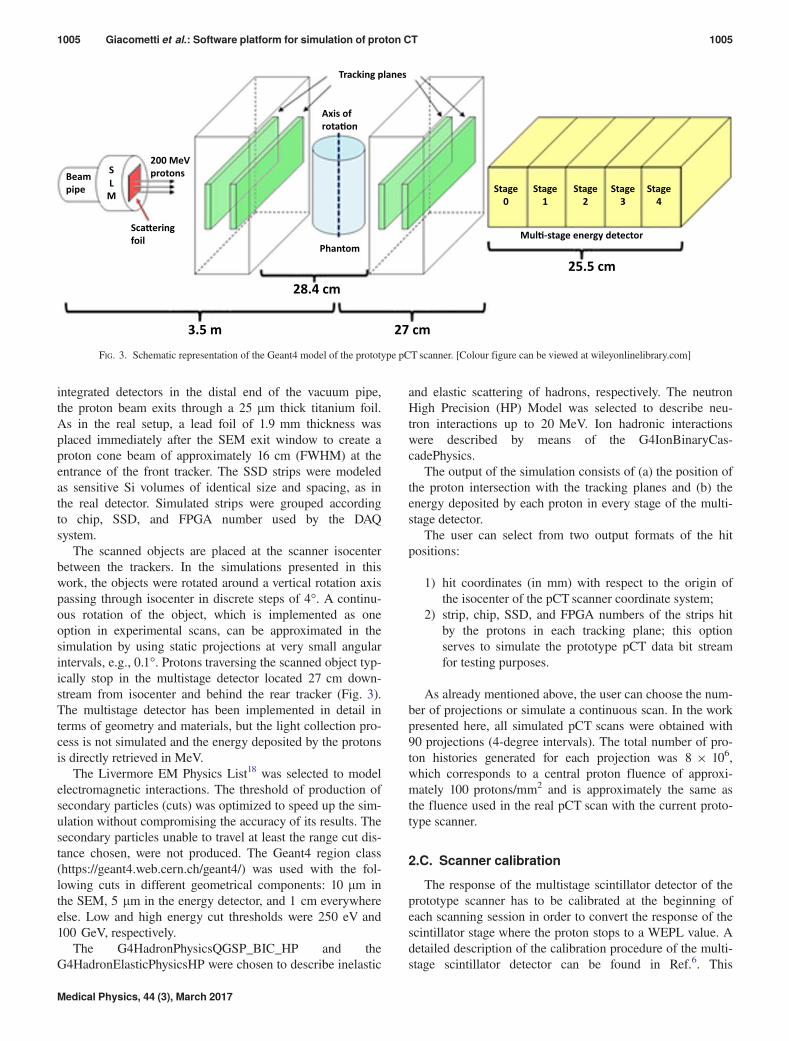
integrated detectors in the distal end of the vacuum pipe,

the proton beam exits through a 25 lm thick titanium foil.

As in the real setup, a lead foil of 1.9 mm thickness was

placed immediately after the SEM exit window to create a

proton cone beam of approximately 16 cm (FWHM) at the

entrance of the front tracker. The SSD strips were modeled

as sensitive Si volumes of identical size and spacing, as in

the real detector. Simulated strips were grouped according

to chip, SSD, and FPGA number used by the DAQ

system.

The scanned objects are placed at the scanner isocenter

between the trackers. In the simulations presented in this

work, the objects were rotated around a vertical rotation axis

passing through isocenter in discrete steps of 4°. A continu-

ous rotation of the object, which is implemented as one

option in experimental scans, can be approximated in the

simulation by using static projections at very small angular

intervals, e.g., 0.1°. Protons traversing the scanned object typ-

ically stop in the multistage detector located 27 cm down-

stream from isocenter and behind the rear tracker (Fig. 3).

The multistage detector has been implemented in detail in

terms of geometry and materials, but the light collection pro-

cess is not simulated and the energy deposited by the protons

is directly retrieved in MeV.

The Livermore EM Physics List18 was selected to model

electromagnetic interactions. The threshold of production of

secondary particles (cuts) was optimized to speed up the sim-

ulation without compromising the accuracy of its results. The

secondary particles unable to travel at least the range cut dis-

tance chosen, were not produced. The Geant4 region class

(https://geant4.web.cern.ch/geant4/) was used with the fol-

lowing cuts in different geometrical components: 10 lm in

the SEM, 5 lm in the energy detector, and 1 cm everywhere

else. Low and high energy cut thresholds were 250 eV and

100 GeV, respectively.

The G4HadronPhysicsQGSP_BIC_HP and the

G4HadronElasticPhysicsHP were chosen to describe inelastic

and elastic scattering of hadrons, respectively. The neutron

High Precision (HP) Model was selected to describe neu-

tron interactions up to 20 MeV. Ion hadronic interactions

were described by means of the G4IonBinaryCas-

cadePhysics.

The output of the simulation consists of (a) the position of

the proton intersection with the tracking planes and (b) the

energy deposited by each proton in every stage of the multi-

stage detector.

The user can select from two output formats of the hit

positions:

1) hit coordinates (in mm) with respect to the origin of

the isocenter of the pCT scanner coordinate system;

2) strip, chip, SSD, and FPGA numbers of the strips hit

by the protons in each tracking plane; this option

serves to simulate the prototype pCT data bit stream

for testing purposes.

As already mentioned above, the user can choose the num-

ber of projections or simulate a continuous scan. In the work

presented here, all simulated pCT scans were obtained with

90 projections (4-degree intervals). The total number of pro-

ton histories generated for each projection was 8 9 106,

which corresponds to a central proton fluence of approxi-

mately 100 protons/mm2 and is approximately the same as

the fluence used in the real pCT scan with the current proto-

type scanner.

2.C. Scanner calibration

The response of the multistage scintillator detector of the

prototype scanner has to be calibrated at the beginning of

each scanning session in order to convert the response of the

scintillator stage where the proton stops to a WEPL value. A

detailed description of the calibration procedure of the multi-

stage scintillator detector can be found in Ref.6. This

Beam

pipe

S200 MeV

protons

Sca�ering

foil

3.5 m 27 cm

25.5 cm

28.4 cm

Phantom

Tracking planes

Stage

0

Stage

1

Stage

2

Stage

3

Stage

4

Axis of

rota�on

Mul�-stage energy detector

L

M

FIG. 3. Schematic representation of the Geant4 model of the prototype pCT scanner. [Colour figure can be viewed at wileyonlinelibrary.com]



https://geant4.web.cern.ch/geant4/

procedure was also simulated in the pCT software platform in

order to realistically reproduce the performance of the pCT

prototype system.

For a single proton, its WEPL is defined as the integral of

the object RSP along the total path length l of the proton

through the object, where the RSP is defined as the ratio of

the stopping power (SP) of a material and the SP of water.

WEPL ¼

Z

l

RSPðEÞdl ¼

Z

l

SPðEÞmaterialSPðEÞwater

dl (1)

In principle, knowing the residual energy of protons, the

WEPL can be calculated by numerically solving the integral

on the right side of Eq. (1) using Bethe–Bloch theory, which

is accurate above 10 MeV.19 Rather than Bethe–Bloch theory,

which requires an assumption about the mean excitation

potential (I), a practical approach consists of calibrating the

energy detector response against known water equivalent

thicknesses (WET) using a calibration phantom with accu-

rately known RSP.5,6 In this work, the calibration was deter-

mined by correlating the signal generated by protons

stopping in the multistage detector to the known thickness

traversed in an ad-hoc polystyrene calibration phantom.

Specifically, Eq. (1) then becomes:

WEPL ¼ x � RSPpolystyrene (2)

where x is the physical thickness traversed in the calibration

phantom and RSPpolystyrene is known to be 1.038 for the cali-

bration phantom used in this work. This calibration procedure

establishes a one-to-one relationship between energy detector

response and WEPL that allows measuring the WEPL of pro-

tons traversing any object, knowing the energy response in

the scintillator stage where they stopped.

The calibration phantom that was implemented in the

Geant4 simulations presented in this work consists of three-

stepped pyramids of polystyrene (Fig. 4) and a variable num-

ber of polystyrene degraders with a relative stopping power

of 1.038. Each pyramid contained eight steps of 6.35 mm

physical thickness adding up to a maximum thickness of

5.08 cm. In order to cover the total range of 200 MeV pro-

tons in polystyrene (25.4 cm), the stepped pyramids (“stairs”)

are combined with a choice of 0, 1, 2, 3, or 4 polystyrene

degraders placed downstream of the stairs. Every degrader

has a physical thickness of 5.08 cm, which is identical to the

maximum thickness of the stairs.

The calibration procedure was simulated with Geant4; to

reproduce the experimental scanning procedure, five calibra-

tion runs with 106 events each were simulated, one with the

stairs alone, and four with the 1, 2, 3, or 4 degraders placed

after the stairs, respectively. The polystyrene thickness tra-

versed by the protons and the energy deposited in each stage

of the multistage detector were recorded for each incident

proton. To avoid ambiguities, protons entering a step of the

stairs within 0.35 mm from its edge were excluded. Also,

protons that were recorded to have entered more than one step

were excluded. Figure 5 shows the simulated geometrical

setup for the calibration with the stairs and four polystyrene

degraders.

For each polystyrene step thickness, the mean energy

deposited in every stage was evaluated with a Gaussian fit

centered approximately in correspondence of the peak of the

histograms of the scintillator responses. Polynomial curves of

energy vs. polystyrene step thickness were fit to those mean

energy values. One should note that with the exception of the

most distal stage, every stage had two types of response: a

response from protons traversing the stage and a response

from protons stopping in the stage. Figure 6 shows simulated

scatter plots of traversed polystyrene thickness vs. energy

deposited in each stage superimposed with polynomial fits of

2nd and 4th degree for responses of each stage to stopping

and traversing protons, respectively. The distinction between

upper segments corresponding to stopping protons and lower

segments corresponding to traversing protons are clearly

FIG. 4. The calibration phantom for the pCT prototype consists of three-

stepped polystyrene pyramids (“stairs”) and a variable set of up to four poly-

styrene degraders; here two degraders behind the stairs are shown. [Colour

figure can be viewed at wileyonlinelibrary.com]

FIG. 5. The Geant4 simulated calibration setup. The silicon detectors are

inside the aluminum cassettes; the parallelepipeds with truncated corners at

PMT ends represents the 5 stages of the multistage scintillator. The calibration

phantom comprised of the stepped pyramids and up to 4 polystyrene degra-

ders are located between the two front and rear trackers. Protons enter the

scanner from the right. [Colour figure can be viewed at wileyonlinelibrary.

com]



seen. The fits to the upper segments were used to convert the

energy deposited in the stage where the proton stopped to

WEPL of the proton. The WEPL was derived using Eq. (2).

Ambiguities arose when the traversed polystyrene thickness

was within � 2 mm of the interface between two stages,

because the signal in the stopping stage may have been pro-

duced by noise, or the proton was not recorded in the stop-

ping stage because the energy deposited could have been

below the experimentally derived noise threshold used in the

simulation (1 MeV). In this case, we applied an empirically

derived weighting formula (3), which was also used for

experimental data,

WEPL ¼ 0:3 �WEPLS þ 0:7 �WEPLT ; (3)

where WEPLS is the WEPL calculated using the calibration

curve of the stage distal to the interface and WEPLT is the

WEPL calculated using the transit segment of the stage proxi-

mal to the interface.

2.D. Image reconstruction

The image reconstruction of pCT aims at calculating a 3D

RSP map of the scanned object from the tracking and WEPL

data for each single proton recorded. Several reconstruction

algorithms, specifically designed for pCT reconstruction,

have been developed and published in recent years.20–22

These algorithms use individual proton histories and calcu-

late their estimated path through the object either based on

the most likely path (MLP) formalism23 or a cubic spline for-

malism.24 A review of iterative pCT image reconstruction

techniques based on projections onto convex sets and MLP

formalism was presented by S.N. Penfold and Y. Censor.7

In the current version of the pCT software platform, the

block-iterative diagonally relaxed orthogonal projections

(DROP) algorithm has been implemented for image recon-

struction of experimental and simulated phantom pCT data.

This image reconstruction algorithm performs feasibility

seeking steps integrated with a total variation superiorization

(TVS) scheme20 and only considers protons entering into and

exiting from the cylindrical reconstruction volume that

enclosed the phantom object. Three-sigma cuts on WEPL,

angle, and vertical and horizontal deviation were imple-

mented to remove protons that underwent large-angle scatter-

ing and/or large energy losses due to inelastic nuclear

interactions. The accepted proton histories were binned into

equal intervals of beam projection angles, lateral coordinates,

and vertical coordinates. The binned data were used as input

to the Feldkamp–Davis–Kress (FDK) algorithm, the cone

beam version of the filter back-projection (FBP) algorithm.

The resulting FBP image was used to define the object

boundary and as the starting point of the iterative reconstruc-

tion algorithm. In brief, WEPL and position and direction of

individual protons traversing the silicon detectors generate a

linear system of equations of the form Ax = b, which is then

solved iteratively with the DROP-TVS algorithm. The ele-

ments aij of the matrix A correspond to the intersection length

of the ith proton with the jth voxel, x is the unknown RSP

vector, and b is the vector of WEPL measurements. The algo-

rithm partitioned the proton histories into 40 blocks, and 8

cycles of iterating through all histories are completed. The

FIG. 6. Scatter plots and calibration curves (lines fitting the square dots) of polystyrene step thickness vs. detector response derived from fitting energy response

distributions to the simulated calibration data. The plots show the polynomial calibration curve segments corresponding to stopping protons (upper segment) and

to traversing protons (lower segment) in each stage, except for stage 4, which only recorded stopping protons. [Colour figure can be viewed at wileyonlinelibrary.-

com]



relaxation parameter of the DROP algorithm was set to 0.1.

The DROP-TVS algorithm was executed on a single graphical

processing unit (GPU) workstation, which is part of a com-

puter cluster at the California State University San Bernar-

dino. The cluster is composed of eight nodes connected with

20 GB Infiniband and 1 GB Ethernet. Each node consists of

a dual 6-core Xeon (48 GB of RAM, 1 TB of Raid, 1.5 TB

of data added storage). A GPU NVIDIA GTX-780 was used

for the image reconstruction.

2.E. pCT software platform validation

The single modules forming the pCT software platform

were validated separately. The Geant4 simulation module was

validated by comparing the tracker detector responses with

experimental measurements. In particular, the horizontal and

vertical proton beam profiles reconstructed from the proton

hit frequencies in all tracking planes were compared. To vali-

date WEPL calibration and conversion modules, the simu-

lated WEPL distributions of protons passing through

polystyrene degraders of three different thicknesses of

50.8 mm, 101.6 mm, and 203.2 mm, respectively, were com-

pared with the experimental WEPL distributions. In addition,

both experimental and simulated mean WEPL values,

obtained from a Gaussian fit to the central part of the distri-

butions, were compared with the expected value of

RSP = 1.038 times the physical thickness of the degraders.

The image reconstruction module of the pCT platform was

validated by comparing reconstructed RSP values with exper-

imental results for a variety of phantoms. Specifically, the

sensitometry module of the Catphan� 600 series was used to

compare both reconstructed experimental and simulated RSP

with the RSP values measured with the PeakFinder (PTW,

Freiburg, Germany) at the Heidelberg Ion-Beam Therapy

Center (HIT). The comparison of simulated and recon-

structed modulation transfer function (MTF) was realized

using the pCT reconstructed images of the line pair module

of the Catphan� 600 series. The HN715 pediatric head phan-

tom was used to compare both reconstructed experimental

and simulated RSP. Operationally, it was not possible to use

the PeakFinder to measure the RSP of the different tissues in

the phantom. Therefore, it was calculated analytically, and a

specific Geant4 simulation was built to collect the data

required in the formula.

2.E.1. Catphan modules image reconstruction

The validation of the performance of the simulated pCT

scanner was performed with the sensitometry and line pair

modules of the Catphan� 600 series (The Phantom Labora-

tory, Salem, NY, USA) and a pediatric anthropomorphic head

phantom (model HN715, CIRS, Norfolk, VA, USA), as

described below.

The CTP 404 sensitometry module (diameter 15 cm) con-

tains eight cylindrical cavities of 1.22 cm diameter, six of

which are filled with different materials, and two that are

filled with air (Fig. 7(a)). The RSP evaluation of the

reconstructed images was conducted with ImageJ version

1.46r, a Java-based open source image-analysis software

package that was downloaded from the US National Institute

of Health website (http://imagej.nih.gov/ij). A circular area of

approximately 1 cm diameter was selected within the bound-

aries of each insert and the mean RSP and standard deviation

were calculated using standard ImageJ functions.

In addition, direct RSP measurements of the six CTP404

inserts were performed at the HITwith the PeakFinder, a vari-

able water column equipped with two plane-parallel ioniza-

tion chambers, each of 4.08 cm radius.25 The WET of each

phantom insert and the phantom body were measured with a

carbon beam of 310.82MeV/u (range 18.02 cm in water) with

4.4 mm FWHM spot size at the isocenter. The measured

RSP values were compared with the RSPs reconstructed from

simulated and experimental pCT data using the iterative

image reconstruction algorithm described in section 2.D. The

use of carbon ions for measuring the WET or RSP of materi-

als valid for protons can be justified by the fact that protons

and heavier ions of similar range have identical WET values

for a given material,26 which was further confirmed with a

separate measurement comparing data obtained with protons

and carbon ions for different tissue equivalent materials using

the same experimental setup. The RSP values obtained for

carbon ions and protons were the same within the accuracy of

the measurements. The advantage of utilizing carbon beams

for the RSP measurements was the smaller spot size and the

reduced multiple Coulomb scattering of the heavier ions

compared to protons, making the measurement more suitable

for the small inserts (12 mm diameter) of the CTP404 mod-

ule. The sharper Bragg peak also allows easier WET interpre-

tation from the measured Bragg curves.

The CTP 528 line pair module (diameter 15 cm) provides

21 groups of high-contrast aluminum bars ranging from 1 to

21 line pairs per cm arranged such that all patterns share the

same distance from the center of the phantom (Fig. 7(b)).

This was used to compare the spatial resolution measured in

images of the phantom reconstructed from simulated data to

those measured in images reconstructed from experimental

pCT data. For quantitative comparison of the spatial resolu-

tion, the MTF was calculated for both cases using a custom-

script written in the Python programming language (https://

www.python.org/). For each of line pair patterns with

lp = 1–5 line pairs, the average reconstructed RSP of the alu-

minum peaks and the average RSP of the base material

troughs were calculated. The MTF for each analyzed line pair

group was then calculated as

MTFðlpÞ ¼

�

RSPpeakðlpÞ�

��

RSPtroughðlpÞ�

�

RSPAl

�

��

RSPbase

� (4)

where�

RSPpeakðlpÞ�

and�

RSPtroughðlpÞ�

are the average

reconstructed RSP values for the aluminum peaks and base

material troughs for a given line pair number, respectively,

and�

RSPAl

�

and�

RSPbase

�

are the energy-averaged RSP val-

ues for aluminum (2.11) and the base material (1.14), respec-

tively, which were calculated as described for head phantom

materials below.



http://imagej.nih.gov/ij

https://www.python.org/

https://www.python.org/

2.E.2. Head phantom image reconstruction

The HN715 pediatric head phantom (Fig. 8(a)) was used

to compare the reconstructed RSP from simulated data and

experimental RSP values of a realistic anatomical object with

each other and with theoretical values based on Bethe–Bloch

theory. This comparison was performed to uncover errors in

the simulation platform including the reconstruction module

when comparing reconstructed RSP from simulated data to

theoretical values. In addition, the comparison of recon-

structed RSP values from simulated and experimental data

was done to provide evidence that the digital head phantom is

a good representation of the actual phantom used in the

experiment. The phantom reproduces anatomical details of

the head and cervical spine of a 5-year-old male (approxi-

mately 13 9 17 cm). The real phantom is composed of tissue

equivalent plastic materials (Fig. 8(b)). The solid material

regions in the phantom were assigned uniform density and

atomic composition (provided by CIRS). The sinus cavities

of the phantom, which in the real phantom are filled with

foamy lung material, were assigned the value of air. The

Geant4 model of the phantom was created using a high-reso-

lution CT scan (GE VTC LightSpeed 64-slice scanner) for

which eight individual scans of 9.6 cm field of view (matrix

512 9 512, pixel size 0.18 mm) and 1.25 mm slice thickness

were stitched together.27 Individual material regions in the

scan were segmented in each slice using the thresholding tool

of ImageJ and then assigned the known material composition

and density. The resulting phantom was assumed to accu-

rately represent the physical phantom, allowing a validation

of the platform performance based on a realistic digital

phantom.

Theoretical absolute stopping power values of each head

phantom material and water were determined using a separate

Geant4 simulation assuming the same material composition

of the head phantom as in the simulation platform. Note that

Geant4 uses Bethe–Bloch theory to calculate the energy loss

of protons when their kinetic energy is higher than 2 MeV.

Monoenergetic protons were tracked inside of a cubic vol-

ume. The threshold of production of secondary particles was

high enough not to generate delta electrons, and energy loss

fluctuation was not included in the simulation. This proce-

dure to calculate the stopping power was described by

Amako et al.28 The stopping power was calculated as the

ratio between energy deposited and the step length in the

first step of protons for energy steps between

E0 = 100 MeV and E1 = 210 MeV using equally spaced

intervals of 0.5 MeV. The stopping power calculated for

each energy step was then fitted with a fourth-degree poly-

nomial, which was integrated to obtain the energy-averaged

stopping power < SPtheo > as:

\SPtheo [ ¼

R E1

E0SPðEÞdER E1

E0dE

(5)

This simulation was performed for each phantom material

and water. The energy-averaged theoretical RSP for each

material (<RSPtheo material>) was then calculated as:

\RSPtheo material [ ¼\SPtheo material [

\SPtheo water [(6)

As before, the RSP calculated from reconstructed simu-

lated and experimental data was determined using ImageJ

with the same procedure used for the CTP 404 sensitome-

try module. As some material regions in the head phantom,

e.g., enamel and cortical bone, had very limited spatial

extension, RSP was calculated by combining the results

from several reconstructed CT slices. For each selected tis-

sue material region, mean RSP and standard deviation were

calculated.

3. RESULTS

3.A. Tracker and multistage scintillator response

For validating the simulated tracker responses, simulated

and experimental horizontal and vertical beam profiles in the

front and rear tracking planes were compared for a run with-

out any phantoms in the beam path. Figure 9 shows a com-

parison between the simulated and experimental tracker

responses to a broad Gaussian-shaped proton beam generated

by the 1.9 mm lead foil, normalized with respect to the total

FIG. 7. (a) Geant4 model of the CTP 404 sensitometry module with the coded materials as indicated. The density of each material, in parenthesis, is expressed in

g/cm3. (b) Geant4 model CTP 528 line pair phantom with aluminum bars embedded in a polymer. Note that the base material of both phantoms is the same.

[Colour figure can be viewed at wileyonlinelibrary.com]



number of histories traversing each tracking plane. As the

t-planes are four time longer than the v-planes, their responses

show a typical Gaussian shape, whereas the responses of the

v-planes only show the central part of the Gaussian profile.

The shapes of the profiles in the respective planes with

horizontal strips (v-planes) and vertical strips (t-planes) was

generally very similar, validating the correctness of the beam

line simulation. During the experiment, the system was care-

fully aligned to the room beam line laser, avoiding shift and

tilt errors relative to the vertical axis. However, the cone beam

axis was slightly tilted relative to the vertical scanner axis in

the experiment causing asymmetry of the beam profile in the

v-planes. The peak of counts at + 40 mm in the first rear

v-planes is caused by noisy strips. Generally, the experimen-

tal tracker response data contain electronic noise that was not

included in the simulation. Therefore, the experimental plot

contains many more noticeable peaks than the simulated

response data. The Geant4 simulation correctly reproduced

the drop in tracking efficiencies due to the vertical gaps in

sensitivity between individual SSDs also seen in the experi-

mental profiles. One should note that the missing coordinates

due to the gaps were reconstructed based on the information

from the other tracking planes and knowledge of the gap

coordinates.29

For validating the simulated multistage scintillator detec-

tor, the simulated WEPL distribution of protons passing

through polystyrene degraders of 50.8 mm, 101.6 mm, and

203.2 mm thickness, respectively, were compared with the

experimental WEPL distributions (Fig. 10). In Table I, the

mean WEPL values calculated for experimental and simu-

lated data are compared with the theoretical values calculated

using equation (2), where x is the physical thickness of the

degraders. The agreement between measured and theoretical

WEPL was within 0.8% both for experimental and simulated

data. The difference between experimental and simulated

WEPL was below 1%.

3.B. Catphan modules

Figure 11 shows the reconstructed images of the CTP 404

sensitometry module using simulated and experimental data

(slices thickness 2.5 mm, reconstructed field of view 18 cm,

pixel size 0.7 mm). Table II shows the comparison between

PeakFinder-measured and reconstructed RSP values (experi-

mental and simulated) for the insertions in the sensitometry

module. The difference between simulated and experimental

RSP is below 1% for all the materials except PMP. The differ-

ence between simulated and experimental RSP for PMP is

1.6%: the simulated RSP is in full agreement with the

expected value, but slightly lower than the experimental one.

Figure 12 shows the correlation between experimental and

simulated RSP and PeakFinder-measured RSP. The coeffi-

cients of determination of 0.9999 for experimental data and

0.9998 for simulated data reflect the excellent predictability

of directly measured RSP values with the reconstructed RSP

values for both simulated and experimental pCT reconstruc-

tions. Finally, even if the difference between simulated and

experimental WEPL is below 1%, the protons stopping in the

interfaces between the scintillators cause different outcomes

in the final WEPL evaluation, as proven by the ring artifacts

in the simulated reconstructed image. The ring artifacts are

related to the calibration of the scanner. In Ref.,30 using simu-

lations with the same scanner geometry, it has been shown

that by replacing the current calibration step phantom with a

wedge phantom, the ring artifacts are reduced to less than

� 0.5% of the surrounding RSP. This has been confirmed

also by recent experiments using a wedge calibration phan-

tom (results not published yet).

Figure 13 shows the reconstructed images of the line pair

module using simulated and experimental data (slices thick-

ness 2.5 mm, reconstructed field of view 18 cm, pixel size

0.7 mm). Figure 14 shows simulated and experimental MTF

calculated for the first five groups of line pairs, where the

(a) (b)

FIG. 8. (a) Anthropomorphic pediatric head phantom model HN715 (CIRS). (b) Geant4 model of the head phantom with color-coded tissue equivalent materials

as indicated. The density of each material, in parenthesis, is expressed in g/cm3. The slice of the head phantom shown does not include spinal disk (1.10 g/cm3).




gaps between the beads are still slightly visible. Simulated

results are slightly higher than experimental MTFs but the

difference never exceeds 0.026 and is always within 1 stan-

dard deviation.

3.C. Head phantom

Figure 15 shows representative reconstructed images of

the pediatric head phantom using simulated and experimental

FIG. 9. Simulated (dashed line) vs experimental (solid line) responses of each tracker plane to a broad Gaussian-shaped proton beam. The two left panels show

the t-plane responses with drops in counts in the graph corresponding to the gaps between SSDs. The right two panels show the v-plane responses; in these cases,

the protons are registered without any dead zones. Note that the horizontal scales in the graphs on the left and on the right are different. [Colour figure can be

viewed at wileyonlinelibrary.com]



data, respectively (slices thickness 1.25 mm, reconstructed

field of view 24 cm, pixel size 0.9 mm). Table III shows the

comparison between experimental and simulated recon-

structed RSP values of the solid tissue equivalent materials of

the pediatric head phantom. The agreement between simu-

lated and experimental reconstructed RSP was found to be

within 1.5%. Cortical bone and spinal disk simulated and

experimental RSPs present a 1.4% of discrepancy. The corti-

cal bone and enamel are very thin (1–2 mm), thus making it

very difficult to select homogeneous regions to measure its

RSP. Moreover, due to limited spatial resolution, such small

regions are not resolved, so the reconstructed RSP values are

FIG. 10. WEPL distribution of one slab (a), two slabs (b), and four slabs (c) of polystyrene using experimental data (solid line) and simulated data (dashed line).


TABLE I. Comparison of experimental, simulated, and theoretical WEPL (eq. 2) from the scan of 1, 2, and 4 polystyrene bricks.

Number of

polystyrene

degraders Thickness [mm]

Theoretical

WEPL [mm]

Experimental WEPL Simulated WEPL

WEPL

Differencec [%]Mean � SD [mm] Differencea [%] Mean � SD [mm] Differenceb [%]

1 50.8 52.73 52.36 � 3.38 �0.70 52.8 � 3.48 0.13 0.84

2 101.6 105.46 104.80 � 3.31 �0.62 105.5 � 3.42 0.03 0.66

4 203.2 210.92 211.12 � 3.17 0.08 211.1 � 3.39 0.08 �0.009

a(Experimental – Theoretical)/Theoretical.b(Simulated – Theoretical)/Theoretical.c(Simulated – Experimental)/Experimental.

(a) (b)

FIG. 11. Catphan� 600 sensitometry module pCT reconstruction using experimental (a) and simulated (b) data. The insertions are: PMP (1), LDPE (2), Polystyr-

ene (3), Epoxy (4), PMMA (5), Delrin (6), Teflon (7), Air (8, 9).



much lower than the theoretical values due to partial volume

averaging with surrounding soft or brain tissue. The spinal

disk was difficult to distinguish from brain in the recon-

structed images causing more uncertainty in its RSP values.

4. DISCUSSION

In this work, validation of a pCT software platform model-

ing a prototype pCT scanner was performed on several levels,

including comparison of the responses of the tracking detec-

tors to the scattered proton cone beam used for imaging, the

response of the five-stage scintillator used to measure the

WEPL of individual protons, and the reconstructed RSP val-

ues of Catphan phantom modules and an anthropomorphic

head phantom.

The simulation software has built-in flexibility in terms of

geometry of the scanner and scanned objects, including the

calibration object, allowing different calibration procedures

to be tested and compared. The reconstruction procedure is

straightforward once the output files are produced using

Geant4 but the reconstruction module can also be changed by

the user allowing different reconstruction algorithms to be

used and added. The work conducted by Dr. Tai Dou at

UCLA shown in Fig. 16 proved the versatility and flexibility

of the simulation software.

The simulation and reconstruction software was previ-

ously developed under an NIH R01 grant to the pCTcollabora-

tion (UCSC, LLU, Baylor University). The pCT Collaboration

maintains a GitHub repository at https://github.com/pCT-col

laboration, where all software code is available to download

by requesting to be added as an outside collaborator. Data files

are available from Baylor University by sending a request

email to [email protected]. A web interface to

request data generated by the platform software or to perform

simulations on the Baylor University computing cluster is

under construction and should be available early 2017.

RSP values of materials inside the different scanned

objects reconstructed from experimental and simulated data

agreed to better than 1.5%. The reconstructed RSP values from

data created by the Geant4 simulation with the pCT software

platform were found in good agreement with theoretical RSP

values, except for those materials that suffered from partial

volume effects due to small geometric dimensions (dentine

and cortical bone in the head phantom). The spatial resolution

limit was of the order of 5 lp/cm for both experimental and

simulated reconstructions with good agreement between the

MTF of both modalities, demonstrating that the simulation

correctly reproduces the factors limiting the spatial resolution

of pCT reconstruction, in particular multiple Coulomb scatter-

ing in the object and the silicon planes.

The computation time necessary to execute the modules of

the simulation platform generally depends on the number of

CPU cores or GPU nodes in the computer/cluster used. With

the computational hardware used in this work, the time

required to run the Geant4 simulation and the WEPL conver-

sion modules for 106 protons was about 24 h. Depending on

the number of cores or GPU nodes available, the time required

to run the image reconstruction module can range from a few

minutes to about 40 min. Further optimization of simulation

TABLE II. Comparison between PeakFinder-measured and experimental and simulated reconstructed RSP values for the materials of the sensitometry module.

(Insert #) Material PF-measured RSP

Reconstructed RSP (experimental) Reconstructed RSP (simulated)

Differencec [%]Mean � SD Differencea [%] Mean � SD Differenceb [%]

(1) PMP 0.883 � 0.002 0.895 � 0.008 1.39 0.880 � 0.003 �0.304 �1.68

(2) LDPE 0.980 � 0.002 0.988 � 0.008 0.91 0.989 � 0.010 1.017 0.10

(3) Polystyrene 1.024 � 0.001 1.033 � 0.005 0.91 1.029 � 0.008 0.519 �0.39

(4) Epoxy 1.144 � 0.001 1.145 � 0.002 0.11 1.154 � 0.009 0.902 0.79

(5) PMMA 1.160 � 0.001 1.162 � 0.003 0.14 1.161 � 0.004 0.058 �0.09

(6) Delrin 1.359 � 0.003 1.360 � 0.002 0.04 1.379 � 0.024 0.190 0.15

(7) Teflon 1.790 � 0.002 1.782 � 0.008 �0.05 1.792 � 0.074 0.098 0.56

a(Experimental – PF-measured)/PF-measured.b(Simulated – PF-measured)/PF-measured.c(Simulated – Experimental)/Experimental.

FIG. 12. Catphan� 600 sensitometry module reconstructed RSP from simu-

lated data (rhomboids) and experimental data (squares). The dotted and

dashed trend lines show the agreement between theoretical and reconstructed

RSP. The number in brackets corresponds to the material labels listed in

Table II and shown in Fig. 11. The coefficient of determination is 0.99 for

both simulated and experimental data. [Colour figure can be viewed at

wileyonlinelibrary.com]



https://github.com/pCT-collaboration

https://github.com/pCT-collaboration

and reconstruction performance are expected to improve com-

puting performance for be acceptable in clinical use.

The pCT software platform can be used as a versatile tool

for studying and improving the performance of clinical pCT

without having access to an experimental pCT scanner. In the

present work, we implemented the experimental proton beam

line at LLUMC. Other beam line models can be implemented

as well, e.g., the Northwester Medicine Chicago Proton Cen-

ter beam line was recently implemented in the pCT software

platform. Note that the possibility of implementing patient

anatomy in the form of DICOM studies within the Geant4

simulation makes it possible to study the feasibility of pCT in

treatment planning and pretreatment plan verification based

on real patients in a virtual fashion. For example, we recently

used the pCT software platform to simulate and reconstruct a

FIG. 14. Catphan�600 Line pair MTF calculated for experimental data (solid

line) and simulated data (dashed line). [Colour figure can be viewed at

wileyonlinelibrary.com]

(a) (b)

FIG. 13. Catphan�60 Line pair module pCT reconstruction using experimental (a) and simulated (b) data.

(a) (b)

FIG. 15. Representative head phantom pCT images reconstructed using experimental (a) and simulated (b) data. The images are approximately through the same

anatomical region.



pCT scan using an imported CT DICOM image of a lung

cancer patient.31 As the existing scanner is only suitable for

head scans, the geometry of the simulation and the proton

energy were changed to accommodate the chest scan. The

space between the two tracking modules was enlarged, and

the active area of the SSDs was increased. In order to pro-

vide sufficient residual energy for all the projection angles,

the proton energy was also increased to 230 MeV. An

additional scintillating stage was added to the multistage

detector to cover the total proton range, and new calibration

curves were defined to convert the energy response into

WEPL. The reconstructed chest image is shown in Fig. 16.

This demonstrates the usefulness using the pCT software

platform to study pCT in new applications and different

anatomical regions. In addition, the pCT software platform

will allow the development and test of new reconstruction

algorithms, for example, for reconstructing 4D pCT image

sets from breathing patients. Moreover, similar to that done

for CBCT,32 the relationship between imaging dose and

related image quality can be studied using the software

platform.

5. CONCLUSION

A modular pCT software platform has been developed and

validated as a model for a prototype pCT scanner. The valida-

tion results presented here show a good agreement between

experimental and simulated data, demonstrating that the sim-

ulation can accurately reproduce the performance of the

actual pCT scanner. The validated platform is a versatile tool

for pCT performance and application studies. The platform is

flexible and can be modified to simulate not only just existing

versions of pCT scanners but also higher proton energies than

those currently clinically available.

ACKNOWLEDGMENTS

We gratefully acknowledge Dr. George Coutrakon from

Northern Illinois University for providing constructive criti-

cism. We acknowledge the kind support by the accelerator

and medical physics staff in the department of the department

of radiation medicine at LLUMC. The use of Kodiak Cluster

at Baylor University was supported by K. E. Schubert, PhD,

B. Schultze, M.S., and B. Sitton B.S., and the use of Akek

Cluster at California State University, San Bernardino, was

supported by Ernesto Gomez, PhD. We thank the University

of Wollongong Information Technology Services (ITS) for

computing time and resources on the UOWHigh Performance

Computing Cluster. We acknowledge that the research in pro-

ton CTwas supported by the National Institute of Biomedical

Imaging and Bioengineering (NIBIB) and the National

Science Foundation (NSF), award Number R01EB013118, and

the United States - Israel Binational Science Foundation

(BSF) grant numbers 2009012 and 2013003.

CONFLICTS OF INTEREST

The authors have no relevant conflicts of interest to

disclose.

a)Author to whom correspondence should be addressed. Electronic mail:

[email protected].

TABLE III. Comparison between RSPs reconstructed from experimental and simulated reconstructed data for the anthropomorphic pediatric head phantom. The

theoretical RSP was calculated using equation (6).

Material Theoretical RSP

Reconstructed RSP (experimental) Reconstructed RSP (simulated)

Differencec [%]Mean � SD Differencea [%] Mean � SD Differenceb [%]

Soft tissue 1.037 1.032 � 0.025 �0.52 1.026 � 0.014 �1.10 �0.58

Brain tissue 1.047 1.044 � 0.08 �0.25 1.043 � 0.012 �0.35 �0.09

Spinal disk 1.060 1.069 � 0.017 0.81 1.053 � 0.039 0.70 �1.50

Trabecular bone 1.108 1.111 � 0.008 0.26 1.110 � 0.020 0.17 �0.09

Cortical bone 1.585 1.331 � 0.032 �16.03 1.312 � 0.082 �17.23 �1.43

Dentin 1.513 1.524 � 0.122 0.72 1.521 � 0.080 0.52 �0.19

Enamel 1.788 1.651 � 0.050 �7.68 1.640 � 0.064 �8.29 �0.67

a(Experimental – Theoretical)/Theoretical.b(Simulated – Theoretical)/Theoretical.c(Simulated – Experimental)/Experimental.

FIG. 16. Proton CT reconstruction of a human chest form pCT software plat-

form data obtained with an imported DICOM xCT phantom (courtesy Dr.

Tai Dou, UCLA).



REFERENCES

1. Clements E. Pursuing protons for medical imaging|symmetry magazine.

2012. [Online]. Available: http://www.symmetrymagazine.org/article/

April-2012/proton-beam-on

2. Hanson KM, Bradbury JN, Cannon TM, et al. Computed tomography

using proton energy loss. Phys Med Biol. 1981;26:965–983.

3. Bashkirov VA, Johnson RP, Sadrozinski HWF, Schulte RW. Develop-

ment of proton computed tomography detectors for applications in

hadron therapy. Nucl Instruments Methods Phys Res Sect A Accel Spec-

trometers Detect Assoc Equip. 2016; 809:120–129.

4. Schulte RW, Bashkirov VA, Li T, et al. Conceptual design of a proton

computed tomography system for applications in proton radiation ther-

apy. IEEE Trans Nucl Sci. 2004;51:866–872.

5. Hurley RF, Schulte RW, Bashkirov VA, et al. Water-equivalent path

length calibration of a prototype proton CT scanner. Med Phys.

2012;39:2438–2446.

6. Bashkirov VA, Schulte RW, Hurley RF, et al. Novel scintillation detec-

tor design and performance for proton radiography and computed

tomography. Med Phys. 2016;43:664–674.

7. Penfold SN, Censor Y. Techniques in iterative proton CT image recon-

struction. Sens Imaging. 2015;16:1–19.

8. Allison J, Amako K, Apostolakis J, et al. Geant4 developments and

applications. IEEE Trans Nucl Sci. 2006;53:270–278.

9. Schulte RW, Bashkirov VA, Johnson RP, Sadrozinski HWF, Schubert

KE. Overview of the LLUMC/UCSC/CSUSB phase 2 proton CT pro-

ject. Trans. Am. Nucl. Soc. 2012;106:59–62.

10. Sadrozinski HWF, Johnson RP, Macafee S, et al. Development of a head

scanner for proton CT. Nucl. Inst. Methods Phys. Res. A. 2013;699:205–210.

11. Sadrozinski HFW, Bashkirov V, Colby B, et al. Detector development for

proton computed tomography (pCT). In: IEEE Nuclear Science Sympo-

sium Conference Record, no. October 2016. Valencia: 2011 IEEE Nuclear

Science SymposiumConference Record (NSS/MIC); 2012: 4457–4461.

12. Johnson RP, DeWitt J, Holcomb C, Macafee S, Sadrozinski HFW, Stein-

berg D. Tracker readout ASIC for proton computed tomography data

acquisition. Psychol Sci. 2013;60:3262–3269.

13. Johnson RP, Bashkirov VA, Dewitt L, et al. A fast experimental scanner

for proton ct: technical performance and first experience with phantom

scans. IEEE Trans Nucl Sci. 2016;63:52–60.

14. Agostinelli S, Allison J, Amako K, et al. GEANT4 – A simulation

toolkit. Nucl Instruments Methods Phys Res Sect A Accel Spectrometers

Detect Assoc Equip. 2003;506:250–303.

15. Allison J, Amako K, Apostolakis J, et al. Recent developments in Gean-

t4. Nucl Instruments Methods Phys Res Sect A Accel Spectrometers

Detect Assoc Equip. 2016;835:186–225.

16. Slater JM, Archambeau JO, Miller DW, Notarus MI, Preston W, Slater

JD. The proton treatment center at Loma Linda University Medical Cen-

ter: rationale for and description of its development. Int J Radiat Oncol

Biol Phys. 1992;22:383–389.

17. Coutrakon G, Hubbard J, Johanning J, Maudsley G, Slaton T, Morton P.

A performance study of the Loma Linda proton medical accelerator.

Med Phys. 1994;21:1691–1701.

18. Chauvie S, Guatelli S, Ivanchenko V, et al. Geant4 low energy electro-

magnetic physics. In: IEEE Symp. Conf. Rec. Nucl. Sci. 2004, Vol. 3, no.

C. Rome: 2004 IEEE Nuclear Science Symposium Conference Record

(NSS/MIC); 2004: 1881–1885.

19. Leo WR. Techniques for nuclear and particle physics experiments : a

how-to approach. Berlin: K, Springer-Verlag, Berlin and Heidelberg

GmbH & Co.; 1994.

20. Penfold SN, Schulte RW, Censor Y, Rosenfeld AB. Total variation supe-

riorization schemes in proton computed tomography image reconstruc-

tion.Med Phys. 2010;37:5887–5895.

21. Penfold SN. The image reconstruction and Monte Carlo simulations in

the development of proton computed tomography for applications in pro-

ton radiation therapy. Wollongong: University of Wollongong Thesis

Collection; 2010.

22. Rit S, Dedes G, Freud N, Sarrut D, L�etang JM. Filtered backprojection

proton CT reconstruction along most likely paths. Med Phys.

2016;40:31103–31109.

23. Schulte RW, Penfold SN, Tafas JT, Schubert KE. A maximum likelihood

proton path formalism for application in proton computed tomography.

Med Phys. 2008;35:4849–4856.

24. Wang D, Mackie TR, Tom�e W. On the use of a proton path probability

map for proton computed tomography reconstruction. Med Phys.

2010;37:4138–4145.

25. Mirandola A, Molinelli S, Vilches Freixas G, et al. Dosimetric commis-

sioning and quality assurance of scanned ion beams at the Italian

National Center for Oncological Hadrontherapy. Med Phys.

2015;42:5287–5300.

26. Zhang R, Taddei PJ, Fitzek MM, Newhauser WD. Water equivalent

thickness values of materials used in beams of protons, helium, carbon

and iron ions. NIH Public Access. 2010;55:2481–2493.

27. Giacometti V, Guatelli S, Bazalova-Carter M, Rosenfeld AB, Schulte

RWM. A high-resolution dicom digital head phantom. Phys Medica.

2017;33:182–188.

28. Amako K, Guatelli S, Ivanchencko V, et al. Validation of Geant4 elec-

tromagnetic physics versus protocol data. In: IEEE Symp. Conf. Rec.

Nucl. Sci. 2004, vol. 4. Rome: 2004 IEEE Nuclear Science Symposium

Conference Record (NSS/MIC); 2004: 1–5.

29. Zatserklyaniy A, Johnson RP, Macafee S, et al. Track Recon-

struction with the Silicon Strip Tracker of the Proton CT Phase

2 Scanner. In: 2014 IEEE Nuclear Science Symposium and

Medical Imaging Conference (NSS/MIC). Seattle: 2014 IEEE

Nuclear Science Symposium Conference Record (NSS/MIC); 2014:

1–4.

30. Piersimoni P, Ramos-Mendez J, Geoghegan T, Bashkirov VA, Schulte

RWM, Faddegon BA. The effect of beam purity and scanner complexity

on proton CT accuracy. Med Phys. 2017;44:284–298.

31. Dou T, Ramos-Mendez J, Piersimoni P, et al. SU-E-J-148: tools

for development of 4D proton CT. Med Phys. Jun. 2015;42:3298–

3299.

32. Yan H, Cervino L, Jia X, Jiang SB. A comprehensive study on the rela-

tionship between the image quality and imaging dose in low-dose cone

beam CT. Phys Med Biol. 2012;57:2063–2080.



http://www.symmetrymagazine.org/article/April-2012/proton-beam-on

http://www.symmetrymagazine.org/article/April-2012/proton-beam-on

software platform for simulation of a prototype … · software platform for simulation of a...

Documents