Software and Manual

Version 2.0

Muhammad N. FaridRalph R. Frerichs

Department of EpidemiologyUniversity of California, Los Angeles (UCLA)

Los Angeles, CA 90095-1772 USA

June, 2007

The CSurvey program was originally programmed for DOS (IBM Compatible computers) byIwan Ariawan of the University of Indonesia while doing graduate studies at UCLA in a programsponsored by the Fogarty International HIV/AIDS Training Program. CSurvey was based on aspreadsheet program that was created by Professor Ralph R. Frerichs and used for many years inhis UCLA course, EPI 418 Rapid Epidemiological Surveys in Developing Countries. Afterattending the EPI 418 course, Muhammad N. Farid, also sponsored by the Fogarty InternationalHIV/AIDS Training Program, designed and programmed Version 2 of Csurvey in Windowsformat. Following creation of Version 2, this manual was written by Professor Frerichs incollaboration with Muhammad Farid.

This manual and software program are in the public domain and may becopied and distributed without restriction. The manual and software program

should not, however, be sold for financial compensation.

-i-

Table of Contents

Chapter 1: Introduction

What is CSurvey? . . . . . . . . . . . . . . . . . . . . . . . . . . . . . . . . . . . . . . . . . . . . . . . . . . . . . . 1.1Cluster selection . . . . . . . . . . . . . . . . . . . . . . . . . . . . . . . . . . . . . . . . . . . . . . . . . . . . 1.1Sample size . . . . . . . . . . . . . . . . . . . . . . . . . . . . . . . . . . . . . . . . . . . . . . . . . . . . . . . 1.1Random number . . . . . . . . . . . . . . . . . . . . . . . . . . . . . . . . . . . . . . . . . . . . . . . . . . . . 1.2

How is this manual organized? . . . . . . . . . . . . . . . . . . . . . . . . . . . . . . . . . . . . . . . . . . . 1.3

Chapter 2: Installation

Obtain from UCLA Epidemiology website . . . . . . . . . . . . . . . . . . . . . . . . . . . . . . . . . . 2.1Install CSurvey on C:drive of computer . . . . . . . . . . . . . . . . . . . . . . . . . . . . . . . . . . . . 2.1Removing CSurvey from computer . . . . . . . . . . . . . . . . . . . . . . . . . . . . . . . . . . . . . . . . 2.5

Chapter 3: Overview Example

Initial sample size . . . . . . . . . . . . . . . . . . . . . . . . . . . . . . . . . . . . . . . . . . . . . . . . . . . . . 3.1Parameter estimation . . . . . . . . . . . . . . . . . . . . . . . . . . . . . . . . . . . . . . . . . . . . . . . . 3.1Hypothesis testing . . . . . . . . . . . . . . . . . . . . . . . . . . . . . . . . . . . . . . . . . . . . . . . . . . 3.4

Preparing for a rapid survey . . . . . . . . . . . . . . . . . . . . . . . . . . . . . . . . . . . . . . . . . . . . . . 3.6Survey parameter . . . . . . . . . . . . . . . . . . . . . . . . . . . . . . . . . . . . . . . . . . . . . . . . . . . 3.8Cluster data . . . . . . . . . . . . . . . . . . . . . . . . . . . . . . . . . . . . . . . . . . . . . . . . . . . . . . . 3.9Sample size check . . . . . . . . . . . . . . . . . . . . . . . . . . . . . . . . . . . . . . . . . . . . . . . . . 3.10

Conducting a rapid survey . . . . . . . . . . . . . . . . . . . . . . . . . . . . . . . . . . . . . . . . . . . . . . 3.12PPS sample at first stage . . . . . . . . . . . . . . . . . . . . . . . . . . . . . . . . . . . . . . . . . . . . 3.12PPS sample at first stage in multi-cluster communities . . . . . . . . . . . . . . . . . . . . . 3.13

Other features . . . . . . . . . . . . . . . . . . . . . . . . . . . . . . . . . . . . . . . . . . . . . . . . . . . . . . . . 3.15Spin dial . . . . . . . . . . . . . . . . . . . . . . . . . . . . . . . . . . . . . . . . . . . . . . . . . . . . . . . . . 3.15Random number . . . . . . . . . . . . . . . . . . . . . . . . . . . . . . . . . . . . . . . . . . . . . . . . . . . 3.17

Chapter 4: Detailed Explanation

Sample size – parameter estimation . . . . . . . . . . . . . . . . . . . . . . . . . . . . . . . . . . . . . . . . 4.1Sample size – hypothesis testing . . . . . . . . . . . . . . . . . . . . . . . . . . . . . . . . . . . . . . . . . . 4.5PPS sample at first stage . . . . . . . . . . . . . . . . . . . . . . . . . . . . . . . . . . . . . . . . . . . . . . . . 4.9

-ii-

-iii-

1.1

Chapter 1: Introduction

What is CSurvey?

CSurvey is a Windows program that performs tasks necessary for conducting rapid surveys,otherwise termed two-stage cluster surveys with probability proportionate to size (PPS) samplingat the first stage and a constant number of households or persons at the second stage. Suchsurveys are typically small (i.e., about 300 households or subjects), although the methods canalso be used for larger surveys. The CSurvey 2.0 program is written for Windows-compatiblemicrocomputers, following the earlier Csurvey1.5 program written in DOS. The program helpsselect a cluster sample from a list of clusters, calculates the sample size for a cluster survey andcreates a random number for selecting random start households or persons within households.There are three main modules in CSurvey.

Cluster selection. The first module selects a sample clusters from a list of all clusters using theprobability proportionate to size (PPS) method. To sample clusters, users must create a sourcedatabase consisting of the name and the size of each cluster in the population to be sampled. Thisdatabase file can be created using CSurvey, or can be imported from other common spreadsheetor database programs. Figure 1.1 shows the selected clusters in a typical source database file.

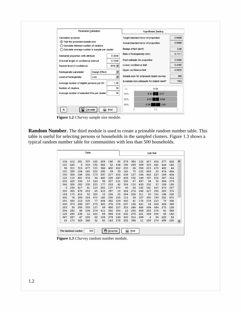
Sample Size. The second module calculates the necessary sample size for a cluster survey tosatisfy the needs of the investigator. Users can evaluate a proposed sample size, or calculate theminimum numbers of clusters or average persons per clusters that are needed for a specifiedconfidence interval. Figure 1.2 shows the sample size calculation for a proposed cluster samplewith prevalence estimate of 50 percent and a 95% confidence interval of 40 to 60 percent or less.

Figure 1.1 CSurvey cluster selection module.

1.2

Random Number. The third module is used to create a printable random number table. Thistable is useful for selecting persons or households in the sampled clusters. Figure 1.3 shows atypical random number table for communities with less than 500 households.

Figure 1.2 CSurvey sample size module.

Figure 1.3 CSurvey random number module.

1.3

How is this manual organized?

Chapter 2 of the CSurvey manual describes how to install the program in a Windows-compatible computer with a C: hard drive that is using the Windows operating system. This isfollowed by Chapter 3 which provides an overview example of a rapid survey which might beplanned for the Yogyakarta region of Indonesia. Those familiar with the DOS version ofCsurvey 1. 5 will likely need no further information to use the new version. Finally, Chapter 4has the technical explanation of the various steps in the CSurvey program, including themathematical formulas that are incorporated into the program.

1.4

2.1

Chapter 2: Installation

Obtain from UCLA Epidemiology Website

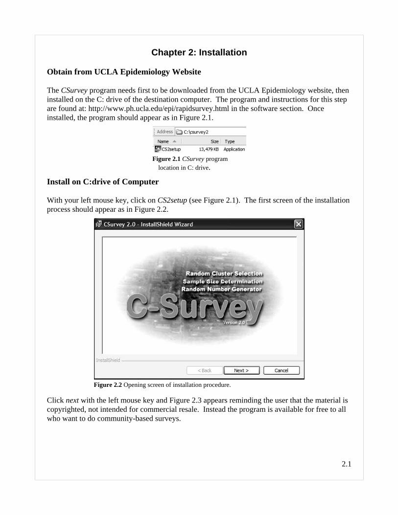
The CSurvey program needs first to be downloaded from the UCLA Epidemiology website, theninstalled on the C: drive of the destination computer. The program and instructions for this stepare found at: http://www.ph.ucla.edu/epi/rapidsurvey.html in the software section. Onceinstalled, the program should appear as in Figure 2.1.

Install on C:drive of Computer

With your left mouse key, click on CS2setup (see Figure 2.1). The first screen of the installationprocess should appear as in Figure 2.2.

Click next with the left mouse key and Figure 2.3 appears reminding the user that the material iscopyrighted, not intended for commercial resale. Instead the program is available for free to allwho want to do community-based surveys.

Figure 2.1 CSurvey programlocation in C: drive.

Figure 2.2 Opening screen of installation procedure.

2.2

Click next again and the screen in Figure 2.4 should appear, showing where the program will beinstalled. If you want a different location, click with the left mouse key on change and enter thenew directory and subdirectory.

Note: in this instance the program is being installed as a subdirectory in C:\ProgramFiles\CSurvey2. The sample files (with the extension *.csf) will also be installed in this

Figure 2.3 Welcome screen of installation process.

Figure 2.4 Destination subdirectory for CSurvey program.

2.3

subdirectory, unless a new location is selected by clicking on Change. If the location is OK,click on Next and continue. Before the installation occurs, the program provides one last chanceto view the destination subdirectory, as shown in Figure 2.5.

The appropriate files are copied by the installation program to the designated location. Whilethis process is occurring, the screen shows the progress being made, as seen in Figure 2.6.

Figure 2.5 Review of destination subdirectory.

Figure 2.6 Installation of CSurvey files.

2.4

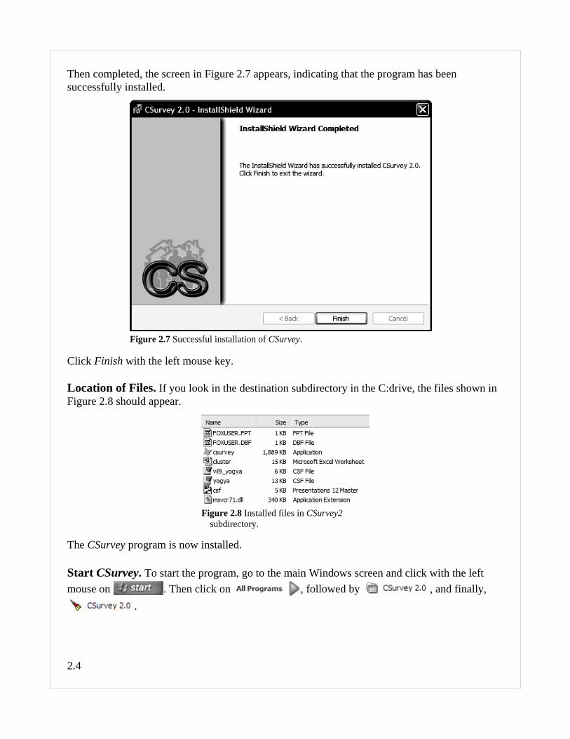
Then completed, the screen in Figure 2.7 appears, indicating that the program has beensuccessfully installed.

Click Finish with the left mouse key.

Location of Files. If you look in the destination subdirectory in the C:drive, the files shown inFigure 2.8 should appear.

The CSurvey program is now installed.

Start CSurvey. To start the program, go to the main Windows screen and click with the leftmouse on . Then click on , followed by , and finally,

.

Figure 2.7 Successful installation of CSurvey.

Figure 2.8 Installed files in CSurvey2subdirectory.

2.5

Removing CSurvey from Computer

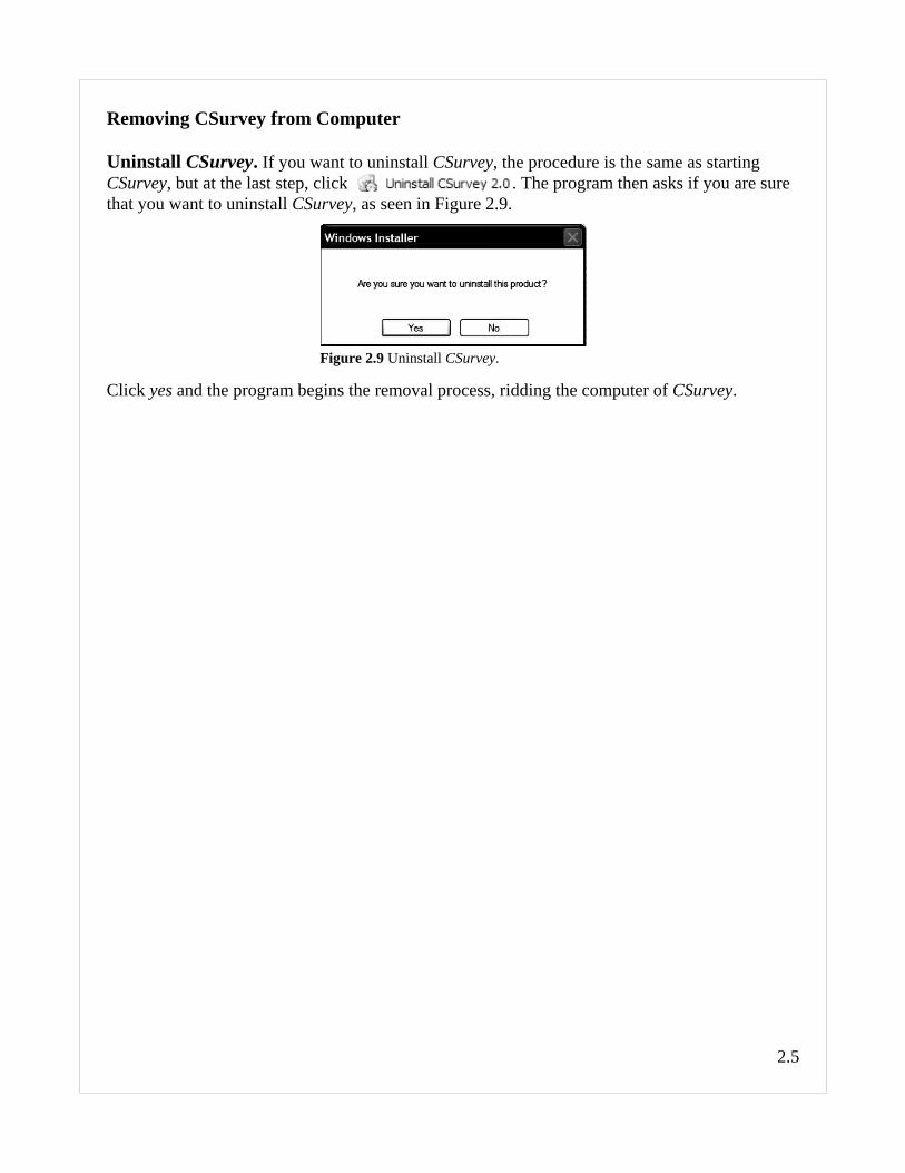
Uninstall CSurvey. If you want to uninstall CSurvey, the procedure is the same as startingCSurvey, but at the last step, click . The program then asks if you are surethat you want to uninstall CSurvey, as seen in Figure 2.9.

Click yes and the program begins the removal process, ridding the computer of CSurvey.

Figure 2.9 Uninstall CSurvey.

2.6

3.1

Chapter 3: Overview Example

Perhaps the easiest way to learn about CSurvey is to step through an example, using data fromIndonesia that are included with the software program. The software is intended to assist withthe various tasks of rapid surveys. More information on rapid surveys is found at:http://www.ph.ucla.edu/epi/rapidsurvey.html.

After starting the CSurvey program (as described at the end of Chapter 2), the screen in Figure3.1 appears.

Assume that you are planning a rapid survey, but have not yet estimated the sample size that is

needed to conduct the survey. To do so, consider the two boxes at the top right of thescreen.

Initial Sample Size

Parameter Estimation. Click with your left mouse key on to create a temporaryworking file termed samplesize.csf, enter the text as shown in Figure 3.2. The click on to create the working file. The screen shown in Figure 3.3 shouldappear.

Figure 3.2 Creation of working file samplesize.csf.

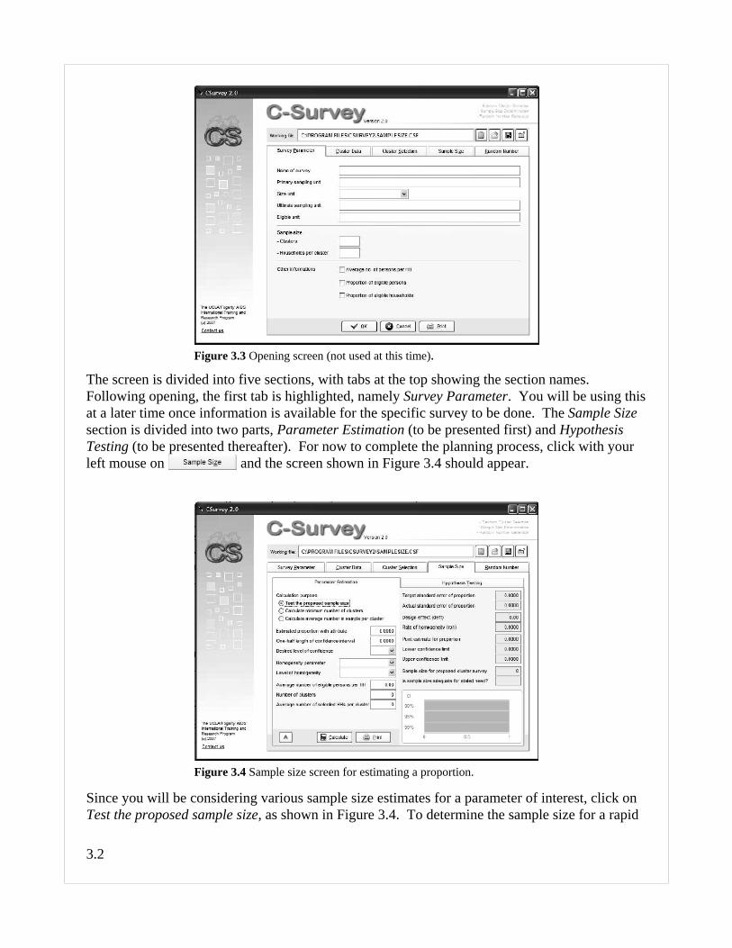
Figure 3.1 CSurvey opening screen.

3.2

Figure 3.4 Sample size screen for estimating a proportion.

The screen is divided into five sections, with tabs at the top showing the section names. Following opening, the first tab is highlighted, namely Survey Parameter. You will be using thisat a later time once information is available for the specific survey to be done. The Sample Sizesection is divided into two parts, Parameter Estimation (to be presented first) and HypothesisTesting (to be presented thereafter). For now to complete the planning process, click with yourleft mouse on and the screen shown in Figure 3.4 should appear.

Since you will be considering various sample size estimates for a parameter of interest, click onTest the proposed sample size, as shown in Figure 3.4. To determine the sample size for a rapid

Figure 3.3 Opening screen (not used at this time).

3.3

survey, you need four values: 1) your best estimate of the proportion with the attribute in thepopulation to be sampled, 2) one-half the length of the maximum confidence interval that wouldbe acceptable (i.e., the desired level of precision), 3) the desired level of confidence (either 90%,95% – the usual level, or 99%), and 4) an estimate of the expected design effect or rate ofhomogeneity. The design effect is a measure of how much greater the variance is of a rapidsurvey (i.e., a two-stage cluster survey) then a similar-sized group with data collected as a simplerandom sample. For immunization surveys, the design effect for sample size estimation is oftenset to 2.0. The rate of homogeneity (or intraclass correlation coefficient) is often used byexperienced surveyors with knowledge of the attribute based on past rapid surveys, while thedesign effect is more commonly used by those without such knowledge.

For this example, assume that about 20% of the sampled population will have the attribute ofinterest; hence, you need to enter 0.20 into the program. Further assume that the maximumacceptable 95% confidence interval is 5 percentage points (i.e., 0.05) or an upper limit of 25%and a lower limit of 15%. Next, assume that the design effect will be low (i.e. 2.0), there will 1.0person per eligible household (a common assumption in immunization surveys of children 12-23months of age), 30 clusters to selected at the first stage, and 10 households with one eligibleperson in each to be selected at the second stage. When through entering the data, click

and Figure 3.5 should appear.

Notice that confidence limits with the specified sample size would be 13.3% and 26.7%, widerthan the 15% and 25% that was requested. To have the desired confidence limits, Figure 3.5shows that the standard error for the estimated parameter should be no greater than 0.0244. Withsample size selected, the actual standard error of the proportion is 0.0327, or too great for the“expectation.” Hence the program answers the question, Is sample size adequate for statedneed? with a “No.” At this point, you can increase the acceptable confidence limits, increase thenumber of clusters, increase the number of selected households per cluster, or with additionalknowledge about the sampling design, reduce the intraclass correlation coefficient towards 0

Figure 3.5 Inadequate sample size for desired confidence limits.

3.4

(the level of a simple random sample) . Assume for now that the size of the desired confidencelimits remains fixed at plus or minus 5 percentage points, and that there are enough funds andtime to sample a larger group, again with 30 clusters, but now set at 18 persons per cluster, asshown in Figure 3.6.

Now the anticipated confidence limits are 15.0% and 25.0%, or at the level acceptable to theinvestigator. Rather than 300 persons being sampled, as in Figure 3.5 however, the sample sizehas now increased to 540 persons. Thus, increased precision has its price, and the cost is paid inincreased time and labor used to sample an additional 240 persons. The small graph at thebottom of the panel shows the expected 90%, 95% and 99% confidence limits, useful forexplaining the concept of confidence limits to persons not intimately familiar with statisticalnotions. If all parties involved with the planned survey deem these values to be acceptable, thenclick on , sign and date the printed page, and leave it with the person or agency that isfunding the planned survey.

Hypothesis Testing. Rather than determining the prevalence or incidence of an attribute in apopulation, you might be interested in comparing a change in an attribute over time, or incomparing the level of an attribute in one region versus another. Such studies are often done toevaluate changes, such as increases in vaccination levels, decreases in smoking behavior,increased use of condoms and the like. To conduct such an evaluation, the program providesinformation on two same-sized rapid surveys, and indicates if the sample size is sufficient todetect a difference in two proportions with an acceptable level of precision, as specified by theinvestigator.

In the Sample Size section, click on Hypothesis Testing in the right side of the panel. Notice thatthe left side of the panel changes, as shown in Figure 3.7.

Figure 3.6 Adequate sample size for desired confidence limits.

3.5

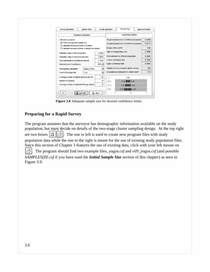
Assume that vaccination coverage is believed to be 20% in one region and 60% in anotherregion, where a more active health care group is at work. Hence, the difference between the tworegions is thought to be 40%. You want to conduct two rapid surveys to test the hypothesis thatthe two regions differ in vaccination coverage. While the investigator or funding agenciesbelieves that the difference between the two regions is 40%, they are willing to accept with 95%confidence that the difference lies between 25% and 55%. That is, with a difference of 0.40 the95% confidence interval should be no greater than ± 0.15. As before the design effect isassumed to be low, the average number of eligible persons per household is assumed to be 1.0,the number of cluster is to be set at 30, and the number of households to be selected per cluster isset at various levels, but shown as 12.

The derived values that fulfill the precision requirements or the investigator or funding agency,are shown in Figure 3.8. As mentioned, the difference between the two proportions is estimatedto be 0.40. Two surveys with 360 subjects in each would result in a 95% confidence interval forthe difference between the two proportions of 0.30 to 0.50, acceptable to the criteria for precisionset by the investigator. Once considered acceptable, the page should be printed, signed, datedand given to the agency or person funding the planned survey.

Figure 3.7 Sample size screen for testing the difference between twoproportions (i.e., hypothesis testing).

3.6

Preparing for a Rapid Survey

The program assumes that the surveyor has demographic information available on the studypopulation, but must decide on details of the two-stage cluster sampling design. At the top rightare two boxes . The one to left is used to create new program files with studypopulation data while the one to the right is meant for the use of existing study population files. Since this section of Chapter 3 features the use of existing data, click with your left mouse on

. The program should find two example files, yogya.csf and vil9_yogya.csf (and possibleSAMPLESIZE.csf if you have used the Initial Sample Size section of this chapter) as seen inFigure 3.9.

Figure 3.8 Adequate sample size for desired confidence limits.

3.7

Select yogya and click on open with the left mouse key, bringing forth the screen shown inFigure 3.10.

The screen is divided into five sections, with tabs at the top showing the section names. Following opening, the first tab is highlighted, namely Survey Parameter.

Figure 3.9 CSF files with CSurvey program.

Figure 3.10 Opening CSurvey screen of yogya.csf, an example file.

3.8

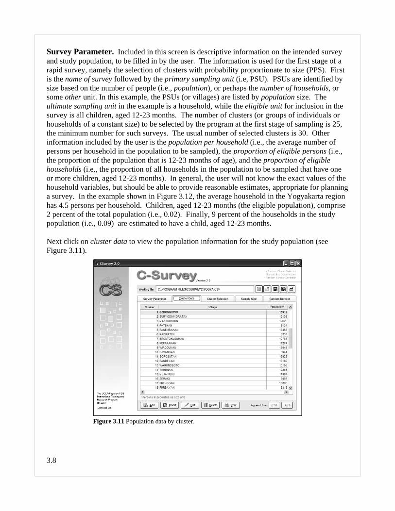
Survey Parameter. Included in this screen is descriptive information on the intended surveyand study population, to be filled in by the user. The information is used for the first stage of arapid survey, namely the selection of clusters with probability proportionate to size (PPS). Firstis the name of survey followed by the primary sampling unit (i.e, PSU). PSUs are identified bysize based on the number of people (i.e., population), or perhaps the number of households, orsome other unit. In this example, the PSUs (or villages) are listed by population size. Theultimate sampling unit in the example is a household, while the eligible unit for inclusion in thesurvey is all children, aged 12-23 months. The number of clusters (or groups of individuals orhouseholds of a constant size) to be selected by the program at the first stage of sampling is 25,the minimum number for such surveys. The usual number of selected clusters is 30. Otherinformation included by the user is the population per household (i.e., the average number ofpersons per household in the population to be sampled), the proportion of eligible persons (i.e.,the proportion of the population that is 12-23 months of age), and the proportion of eligiblehouseholds (i.e., the proportion of all households in the population to be sampled that have oneor more children, aged 12-23 months). In general, the user will not know the exact values of thehousehold variables, but should be able to provide reasonable estimates, appropriate for planninga survey. In the example shown in Figure 3.12, the average household in the Yogyakarta regionhas 4.5 persons per household. Children, aged 12-23 months (the eligible population), comprise2 percent of the total population (i.e., 0.02). Finally, 9 percent of the households in the studypopulation (i.e., 0.09) are estimated to have a child, aged 12-23 months.

Next click on cluster data to view the population information for the study population (seeFigure 3.11).

Figure 3.11 Population data by cluster.

3.9

For any rapid survey, such population data needs to be entered by the investigator for allcommunities in the study population. To do so, the person conducting the survey can create forthe population to be sampled a new *.csf file, append an earlier-created *.csf (see bottom right ofFigure 3.11), or created and append a *.xls file using the spreadsheet program, MS Excel (alsosee bottom right of Figure 3.11). If planning to use the MS Excel option, a screen appears thatguides the data entry process, as seen in Figure 3.12.

Cluster Data. The example data set shown in Figure 3.11 contains information on 45 villages,with the estimated population presented in the column at right. The data are easily edited orprinted, using the keys at the bottom of the screen.

To make sure that the sample size specified in Figure 3.10 is adequate to fulfill the needs of theinvestigator, click on the tab sample size, as shown in Figure 3.13.

Figure 3.12 Format for importing data from MS Excel.

3.10

Sample Size Check. In this example, the attribute being surveyed has an estimated proportionvalue of 0.20 (or percentage value of 20%). The investigator is willing to accept 95%confidence limits of .12 to .28 (or 12 to 28%); that is, one half of the confidence interval size is0.08. Being a cluster survey, the variance estimate will likely be larger than if done as a simplerandom sample survey. How much larger is estimated by either the design effect or the rate ofhomogeneity. In the example, the design effect is selected and the estimated value is set as low,which is equivalent to a design effect of 2.0. A small survey is specified, of 25 clusters and 10children aged 12-23 months. For the Indonesia example, the 10 sampling units per cluster are 10households with one or more 12-23 month olds. Is this sample size adequate? To make sure,click on (which imports the appropriate information from Survey Parameter) followed by

.

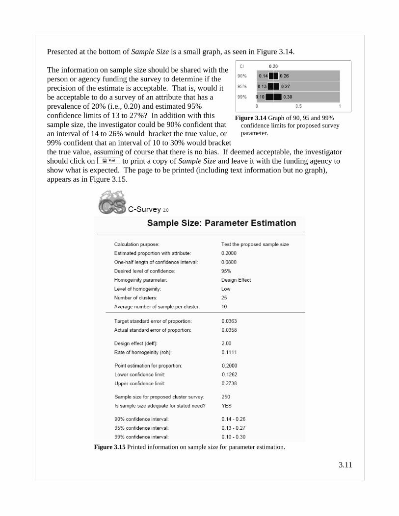
In the example in Figure 3.13, the sample size for the proposed survey would be 250 persons, or25 clusters with 10 eligible households per cluster with 1.0 child, aged 12-23 months, in eacheligible household. In this example, the target standard error of the proportion needed to be nomore than 0.0363 to fulfil the criteria entered in the first column of Sample Size by theinvestigator. Based on the estimated sample size, the standard error of the proportion is 0.0358,less than the target maximum of 0.0363. Hence, the proposed sample size is adequate for thestated need, and the program responds yes. With a “low” level of homogeneity (as selected bythe investigator), the program assumes a design effect of 2.0 (i.e., the variance of the clustersurvey will be twice as great as the variance of a similar-sized survey done as a simple randomsample) and have a rate of homogeneity of 0.1111. The mean and 95% confidence limits areestimated as a proportion as 0.2000 (0.1262, 0.2738), or as a percentage as 20% (12.6%, 27.4%).

Figure 3.13 Check of specified sample size for two-stage cluster survey.

3.11

Presented at the bottom of Sample Size is a small graph, as seen in Figure 3.14.

The information on sample size should be shared with theperson or agency funding the survey to determine if theprecision of the estimate is acceptable. That is, would itbe acceptable to do a survey of an attribute that has aprevalence of 20% (i.e., 0.20) and estimated 95%confidence limits of 13 to 27%? In addition with thissample size, the investigator could be 90% confident thatan interval of 14 to 26% would bracket the true value, or99% confident that an interval of 10 to 30% would bracketthe true value, assuming of course that there is no bias. If deemed acceptable, the investigatorshould click on to print a copy of Sample Size and leave it with the funding agency toshow what is expected. The page to be printed (including text information but no graph),appears as in Figure 3.15.

Figure 3.14 Graph of 90, 95 and 99%confidence limits for proposed surveyparameter.

Figure 3.15 Printed information on sample size for parameter estimation.

3.12

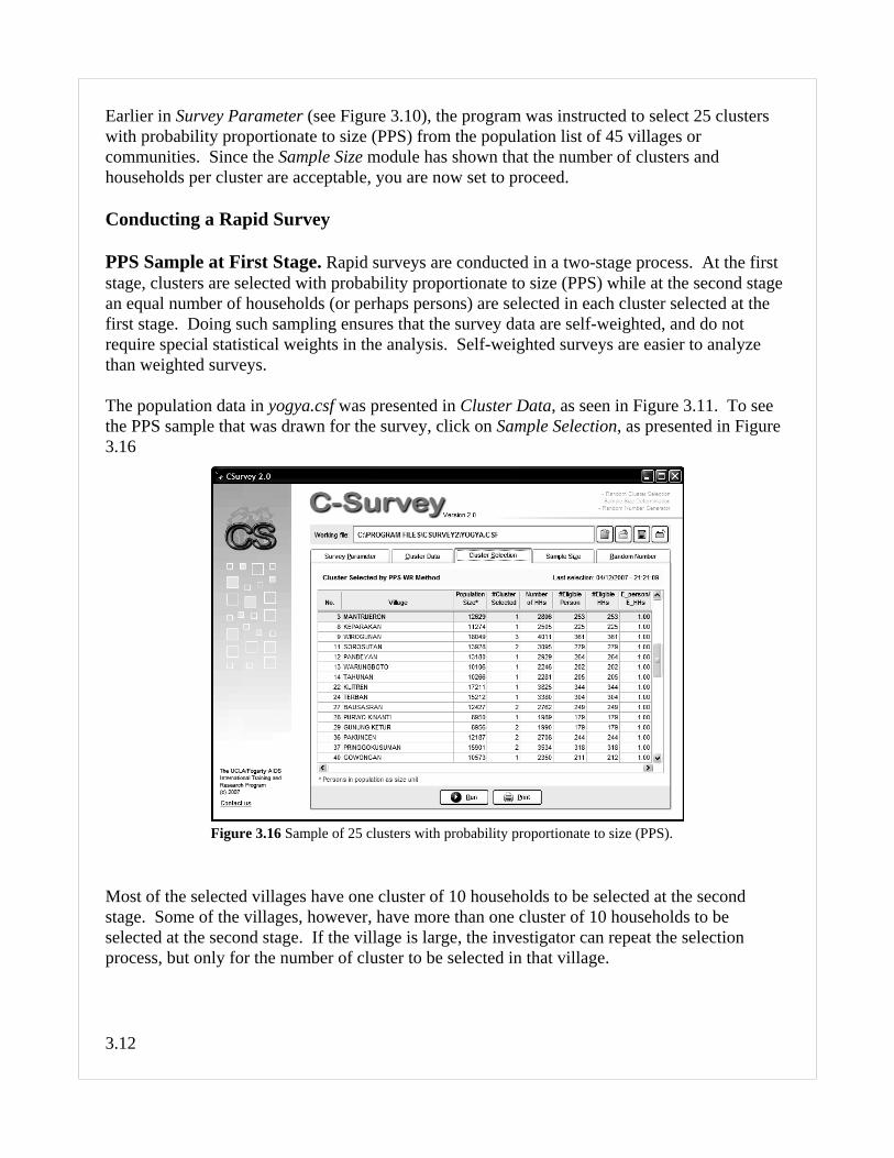
Earlier in Survey Parameter (see Figure 3.10), the program was instructed to select 25 clusterswith probability proportionate to size (PPS) from the population list of 45 villages orcommunities. Since the Sample Size module has shown that the number of clusters andhouseholds per cluster are acceptable, you are now set to proceed.

Conducting a Rapid Survey

PPS Sample at First Stage. Rapid surveys are conducted in a two-stage process. At the firststage, clusters are selected with probability proportionate to size (PPS) while at the second stagean equal number of households (or perhaps persons) are selected in each cluster selected at thefirst stage. Doing such sampling ensures that the survey data are self-weighted, and do notrequire special statistical weights in the analysis. Self-weighted surveys are easier to analyzethan weighted surveys.

The population data in yogya.csf was presented in Cluster Data, as seen in Figure 3.11. To seethe PPS sample that was drawn for the survey, click on Sample Selection, as presented in Figure3.16

Most of the selected villages have one cluster of 10 households to be selected at the secondstage. Some of the villages, however, have more than one cluster of 10 households to beselected at the second stage. If the village is large, the investigator can repeat the selectionprocess, but only for the number of cluster to be selected in that village.

Figure 3.16 Sample of 25 clusters with probability proportionate to size (PPS).

3.13

PPS Sample at First Stage in Multi-Cluster Communities. An example follows for 9.Wirogunan which is shown in Figure 3.16 (line 3) as a village that has three cluster to beselected. To this end, the village of Wirogunan has been further divided, making the processeasier on the field team. To see the data for the Wirogunan village, click on followed byvil9_yogya.csf and ; Figure 3.17 should appear. Notice that the figure shows there arethree clusters to be selected, not 25 as before, but still features 10 households per cluster. Theremaining information about household size and the like is the same as in Figure 3.10.

To see the data for the village of Wirogunan, click on Cluster Data at the top of the panel. Figure 3.18 should appear.

Figure 3.17 Sample of 3 clusters in village Wirogunan.

3.14

The five sub-regions total 18,049, the population of Wirogunan, shown before in Figure 3.16. To select the three clusters in Wirogunan that were originally indicated in Figure 3.16, click onCluster Selection. As seen in Figure 3.19, three of the five sub-regions now have one clusterselected in each.

The same procedure can be repeated for the other villages where more than one cluster wasselected. Alternatively, the villages could have been sub-divided earlier into small units so thatone cluster is likely to be selected in each, but this might entail too much data gathering,entering, and tallying time.

Figure 3.18 Sub-regions in village Wirogunan.

Figure 3.19 PPS sample of thee clusters in sub-regions of Wirogunan.

3.15

Other Features

There are two additional features in the CSurvey program that are useful for doing rapid surveys. These are a random-direction spin dial and the generation of a random number table.

In many regions of the world, households are not clearly identified or numbered. In suchsituations, the most common procedure for selecting a constant number of households (oreligible subjects) at the second stage is first to obtain a random start household, and thencontinue to the next nearest neighbor until the constant quota is met. The intention is for eachhousehold in the cluster to have an equal chance of becoming the random start household. Theprocedure has the surveyor start at the center of the selected village or sub-region. Next, he orshe spins a dial to select a random direction to walk to the periphery of the village or sub-region(i.e., a randomly selected vector), and counts all the households passed along the directed vector(see Figure 3.20). The passed households are marked and numbered on a map form, sketched byhand in the field.

Once all the households along the chosen vector are counted and marked on the map form, oneof them is selected by sampling from a list of random numbers, specifically a number between 1and the last house counted (i.e., #10 in the example). The selected household is deemed therandom start household and is the starting point for obtaining the constant number of eligiblehouseholds (or persons, if one eligible person per household) for the cluster.

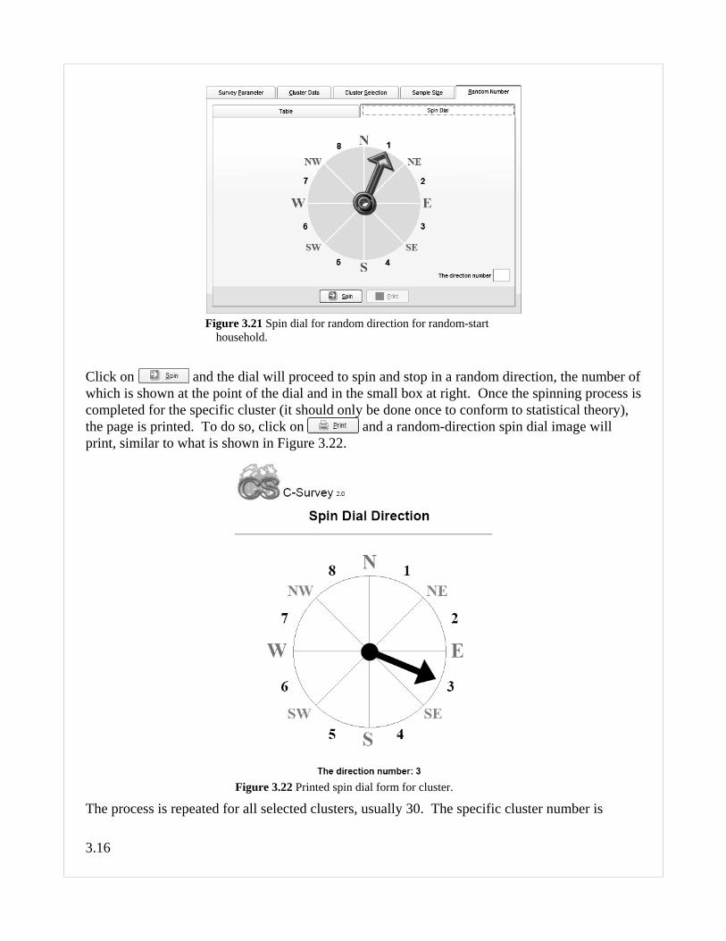
Spin Dial. Click on Random Number at the top of the panels, followed by Spin Dial (the sectionto the right), as presented in Figure 3.20. Notice that the dial is divided into 8 numbered slices ofa circular pie.

Figure 3.20 Count households along random vector toperiphery.

3.16

Click on and the dial will proceed to spin and stop in a random direction, the number ofwhich is shown at the point of the dial and in the small box at right. Once the spinning process iscompleted for the specific cluster (it should only be done once to conform to statistical theory),the page is printed. To do so, click on and a random-direction spin dial image willprint, similar to what is shown in Figure 3.22.

The process is repeated for all selected clusters, usually 30. The specific cluster number is

Figure 3.21 Spin dial for random direction for random-starthousehold.

Figure 3.22 Printed spin dial form for cluster.

3.17

written at the top of the form and the page is given to the appropriate interviewer/examiner. With this page, the field persons needs only a small, inexpensive compass to determine thedirection of the random vector. Using the compass, the field worker determines north, thenwalks along an imaginary line in the random direction shown on the spin dial (i.e., #3 in theexample) towards the periphery of the village or sub-region. All households passed along theway are counted and listed on the map form, as previously shown in Figure 3.20.

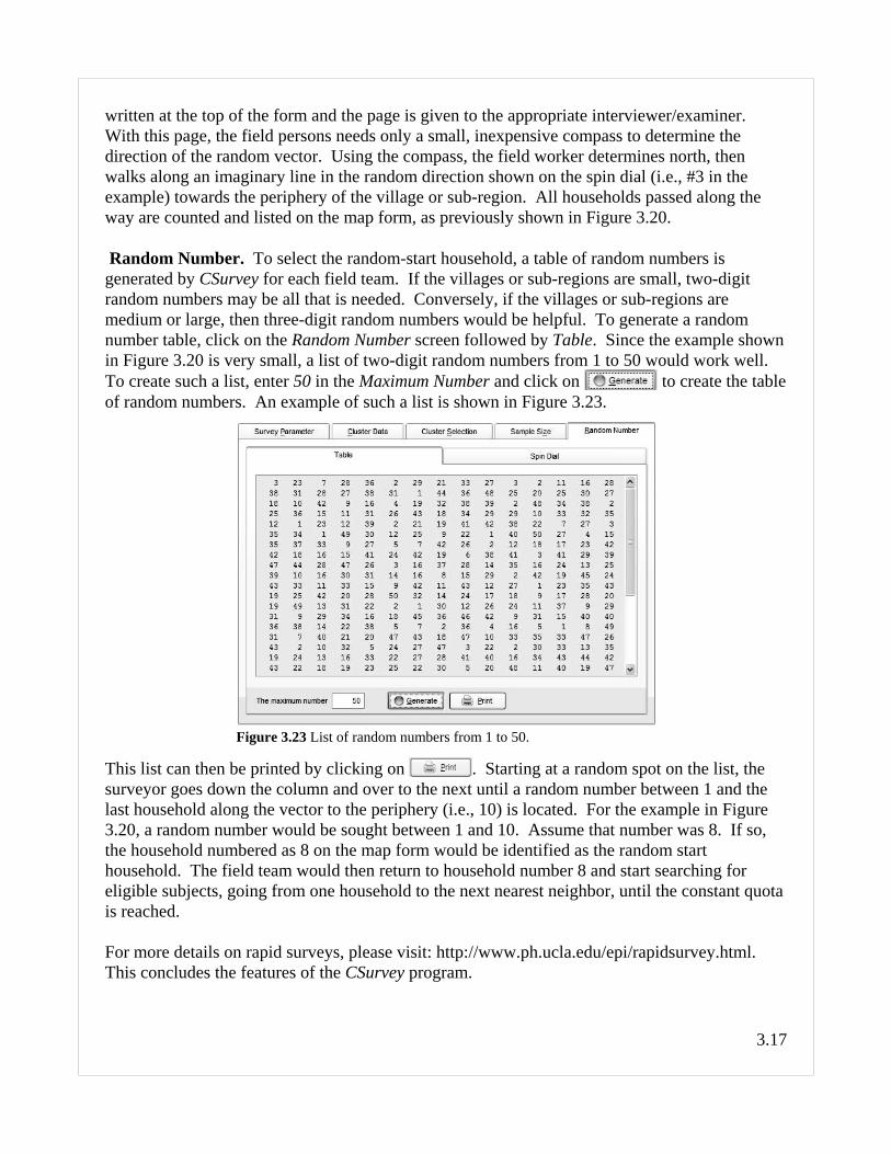
Random Number. To select the random-start household, a table of random numbers isgenerated by CSurvey for each field team. If the villages or sub-regions are small, two-digitrandom numbers may be all that is needed. Conversely, if the villages or sub-regions aremedium or large, then three-digit random numbers would be helpful. To generate a randomnumber table, click on the Random Number screen followed by Table. Since the example shownin Figure 3.20 is very small, a list of two-digit random numbers from 1 to 50 would work well. To create such a list, enter 50 in the Maximum Number and click on to create the tableof random numbers. An example of such a list is shown in Figure 3.23.

This list can then be printed by clicking on . Starting at a random spot on the list, thesurveyor goes down the column and over to the next until a random number between 1 and thelast household along the vector to the periphery (i.e., 10) is located. For the example in Figure3.20, a random number would be sought between 1 and 10. Assume that number was 8. If so,the household numbered as 8 on the map form would be identified as the random starthousehold. The field team would then return to household number 8 and start searching foreligible subjects, going from one household to the next nearest neighbor, until the constant quotais reached.

For more details on rapid surveys, please visit: http://www.ph.ucla.edu/epi/rapidsurvey.html.This concludes the features of the CSurvey program.

Figure 3.23 List of random numbers from 1 to 50.

4.1

Chapter 4: Detailed Explanation

This chapter provides a brief, but detailed, explanation of each procedure featured in CSurvey. Foradditional information on rapid surveys, please go to: http://www.ph.ucla.edu/epi/rapidsurvey.html.

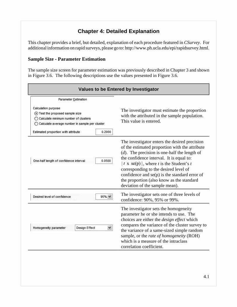
Sample Size - Parameter Estimation

The sample size screen for parameter estimation was previously described in Chapter 3 and shownin Figure 3.6. The following descriptions use the values presented in Figure 3.6.

Values to be Entered by Investigator

The investigator must estimate the proportionwith the attributed in the sample population.This value is entered.

The investigator enters the desired precisionof the estimated proportion with the attribute(d). The precision is one-half the length ofthe confidence interval. It is equal to:

, where t is the Student’s tcorresponding to the desired level ofconfidence and se(p) is the standard error ofthe proportion (also know as the standarddeviation of the sample mean).

The investigator sets one of three levels ofconfidence: 90%, 95% or 99%.

The investigator sets the homogeneityparameter he or she intends to use. Thechoices are either the design effect whichcompares the variance of the cluster survey tothe variance of a same-sized simple randomsample, or the rate of homogeneity (ROH)which is a measure of the intraclasscorrelation coefficient.

4.2

The investigator sets the anticipated level ofthe homogeneity parameter. The choices aresame as a simple random sample (i.e., eithera design effect of 1.0 or the equivalent ROH),low (i.e., either a design effect of 2.0 or theequivalent ROH), medium (i.e., either adesign effect of 4.0 or the equivalent ROH),high (i.e., either a design effect of 7.0 or theequivalent ROH), or manual (i.e., set by theinvestigator).

The investigator either enters an estimate of the average number of eligible persons whoreside in a household, or has the programprovide this value based on informationentered in the Survey Parameter screen (seeFigure 3.10).

The enters the number of cluster to besampled at the first stage with probabilityproportionate to size (PPS) – shown here asthe typical value of 30. This number shouldbe 25 or greater to conform to statisticaltheory regarding an unbiased parameterestimate.

The investigator enters the constant numberof households (or persons, if one person pereligible household) to be selected in eachchosen cluster.

Once the investigator has entered the various values, the program calculates the correspondingsample values that go with the investigator’s entries. As previously, the presentation is based onvalues shown earlier in Figure 3.6.

4.3

Values Derived by the Program

Based on the entered values, the programdetermines the maximum standard error thatwould fulfil the wishes of the investigator. The value is the desired level of precision (d)divided by the value of the Student’s t thatcorresponds to 1 minus the number of

clusters. That is, .

The program calculates the standard errorbased on the entered values, the formula ofwhich is:

,

where p is the proportion with the attribute, qis 1-p, roh is the rate of homogeneity (orintraclass correlation coefficient), is themean number of persons per cluster, and n isthe number of clusters.

Based on entered value of the investigator theprogram calculates the design effect. If rohwas entered, rather than the design effect(deff), the program calculates the designeffect using the formula:

, where is asdefined above.

The rate of homogeneity (roh) is either thevalue entered by the investigator as a measureof the intraclass correlation coefficient, or is

derived by: , where deff, and

are as previously defined.

The point estimate (p) was previously enteredby the investigator and is again shown here.

4.4

The upper and lower confidence limits for thedesired confidence interval (CI) are derivedas: , where p is the pointestimate, t is the Student’s t corresponding to1 minus the number of clusters (i.e., thedegrees of freedom for the analysis of a ratioestimator), and se(p) is the standard error ofthe proportion.

The sample size being proposed by theinvestigator is equal to: , where n is thenumber of clusters and is the mean numberof persons per cluster.

The program compares the derived se(p) tothe target se(p) based on the wishes of the

investigator and enters “yes” if or

“no” if , where se(p) is the

standard error of the proportion, d is one-halfthe length of the confidence interval and t isthe value of the Student’s t corresponding to 1minus the number of clusters.

Finally, the program derives 90, 95 and 99%confidence intervals for the proposed sample.The formula for the confidence interval is

. For the example of 30clusters (i.e., 29 degrees of freedom in thecoming statistical analysis), the values of t are1.699 for the 90% CI, 2.045 for the 95% CIand 2.756 for the 99% CI. The values of tused by the program are dependent on thenumber of clusters entered by theinvestigator. If the lower confidence limit isless than 0 or the upper confidence limit isgreater than 1, the values are truncated to 0and 1, respectively.

The program also calculates the minimum number of clusters that would be needed to fulfill theinvestigator’s wishes (assuming the average number of eligible persons per household and averagenumber of households per cluster are included) or the average number in sample per cluster(assuming the average number of eligible persons per household and number of clusters are

4.5

included).

Sample Size - Hypothesis Testing

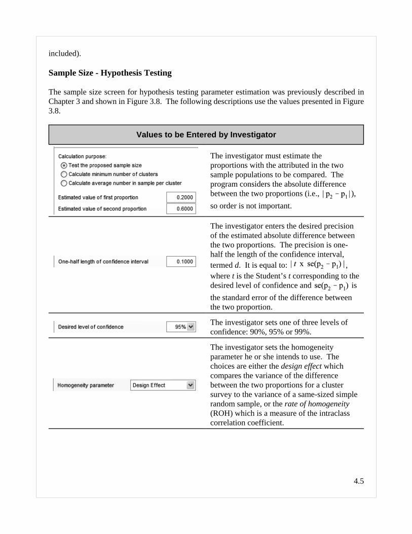
The sample size screen for hypothesis testing parameter estimation was previously described inChapter 3 and shown in Figure 3.8. The following descriptions use the values presented in Figure3.8.

Values to be Entered by Investigator

The investigator must estimate theproportions with the attributed in the twosample populations to be compared. Theprogram considers the absolute differencebetween the two proportions (i.e., ),so order is not important.

The investigator enters the desired precisionof the estimated absolute difference betweenthe two proportions. The precision is one-half the length of the confidence interval,termed d. It is equal to: ,where t is the Student’s t corresponding to thedesired level of confidence and isthe standard error of the difference betweenthe two proportion.

The investigator sets one of three levels ofconfidence: 90%, 95% or 99%.

The investigator sets the homogeneityparameter he or she intends to use. Thechoices are either the design effect whichcompares the variance of the differencebetween the two proportions for a clustersurvey to the variance of a same-sized simplerandom sample, or the rate of homogeneity(ROH) which is a measure of the intraclasscorrelation coefficient.

4.6

The investigator sets the anticipated level ofthe homogeneity parameter for the differencebetween the two proportions. The choices aresame as a simple random sample (i.e., eithera design effect of 1.0 or the equivalent ROH),low (i.e., either a design effect of 2.0 or theequivalent ROH), medium (i.e., either adesign effect of 4.0 or the equivalent ROH),high (i.e., either a design effect of 7.0 or theequivalent ROH), or manual (i.e., set by theinvestigator).

The investigator either enters an estimate of the average number of eligible persons whoreside in a household, or has the programprovide this value based on informationentered in the Survey Parameter screen (seeFigure 3.10).

The enters the number of cluster to besampled at the first stage with probabilityproportionate to size (PPS) in the twosurveys. In the example, each survey has 30clusters selected, for a total of 60 clusters.

The investigator enters the constant numberof households (or persons, if one person pereligible household) to be selected in eachchosen cluster in the two surveys.

Once the investigator has entered the various values, the program calculates the correspondingsample values that go with the investigator’s entries.

4.7

Values Derived by the Program

Based on the entered values, the programderives the maximum standard error of thedifference between two proportions thatwould fulfil the wishes of the investigator. The value is the desired level of precision (d)divided by the value of the Student’s t thatcorresponds to 1 minus the number of clusters

in each survey. That is, .

The program calculates the standard errorbased on the entered values, the formula ofwhich is:

,

where and are the two proportions withthe attribute, and are and ,respectively, deff is design effect, n is thenumber of clusters in each of the two surveys,and is the mean number of persons percluster in each of the two surveys.

Based on entered value of the investigator theprogram calculates the design effect. If rohwas entered, rather than the design effect(deff), the program calculates the designeffect using the formula:

, where is asdefined above.

The rate of homogeneity (roh) is either thevalue entered by the investigator as a measureof the intraclass correlation coefficient, or is

derived by: , where deff, and

are as previously defined.

The two point estimates (i.e., and ) werepreviously entered by the investigator and isshown here as or .

4.8

The upper and lower confidence limits for thedesired confidence interval (CI) are derivedas: , where

and are the two point estimates, t is theStudent’s t corresponding to 1 minus thenumber of clusters, and is thestandard error of the difference between thetwo proportions.

The sample size being proposed by theinvestigator for each of the two clustersurveys is equal to: , where n is thenumber of clusters and is the mean numberof persons per cluster. The total in theexample for the two surveys is 720.

The program compares the derivedto the target based on

the wishes of the investigator and enters

“yes” if or “no” if

, where is the

standard error of the difference between thetwo proportions, d is one-half the length ofthe confidence interval and t is the value ofthe Student’s t corresponding to 1 minus thenumber of clusters.

Finally, the program derives 90, 95 and 99%confidence intervals for the proposed sample.The formula for the confidence interval is

. For theexample of 30 clusters (i.e., 29 degrees offreedom in the coming statistical analysis),the values of t are 1.699 for the 90% CI,2.045 for the 95% CI and 2.756 for the 99%CI. The values of t used by the program aredependent on the number of clusters enteredby the investigator.

The program also calculates the minimum number of clusters that would be needed to fulfill the

4.9

investigator’s wishes (assuming the average number of eligible persons per household and averagenumber of households per cluster are included) or the average number in sample per cluster(assuming the average number of eligible persons per household and number of clusters areincluded).

PPS sample at first stage

For rapid surveys (i.e., two stage cluster surveys), clusters (villages, communities, city blocks, etc)are selected at the first stage with probability proportionate to size. Once the population data isentered for each cluster, the program creates a cumulative list of the total sample population, andretains the location of each cluster in the cumulative list. A random number is then selected between1 and the total sample population. The number is then assigned to the corresponding cluster in thecumulative list. The process is repeated for each of the clusters, typically 30. Hence the clustersare drawn randomly with probability proportionate to size (PPS), with replacement.

This ends Chapter 4 and the Csurvey Manual.