atmosphere

Article

Sodium Resonance Wind-Temperature Lidar at PFRR:Initial Observations and Performance

Jintai Li 1, Bifford P. Williams 2 , Jennifer H. Alspach 3 and Richard L. Collins 3,*1 Department of Physics and Astronomy, Clemson University, Clemson, SC 29634, USA; jintail@g.clemson.edu2 GATS, Boulder, CO 80301, USA; b.p.williams@gats-inc.com3 Geophysical Institute and Department of Atmospheric Sciences, University of Alaska Fairbanks, Fairbanks,

AK 99775, USA; jalspach@alaska.edu* Correspondence: rlcollins@alaska.edu

Received: 4 December 2019; Accepted: 1 January 2020; Published: 15 January 2020�����������������

Abstract: A narrowband sodium resonance wind-temperature lidar (SRWTL) has been deployed atPoker Flat Research Range, Chatanika, Alaska (PFRR, 65◦ N, 147◦W). Based on the Weber narrowbandSRWTL, the PFRR SRWTL transmitter was upgraded with a state-of-the-art solid-state tunable diodelaser as the seed laser. The PFRR SRWTL currently makes simultaneous measurements in the zenithand 20◦ off-zenith towards the north with two transmitted beams and two telescopes. Initial resultsfor both nighttime and daytime measurements are presented. We review the performance of the PFRRSRWTL in terms of seven previous and currently operating SRWTLs. The transmitted power fromthe pulsed dye amplifier (PDA) is comparable with other SRWTL systems (900 mW). However, whilethe efficiency of the seeding and frequency shifting is comparable to other SRWTLs the efficiency ofthe pumping is lower. The uncertainties of temperature and wind measurements induced by photonnoise at the peak of the layer with a 5 min, 1 km resolution are estimated to be ~1 K and 2 m/s fornighttime conditions, and 10 K and 6 m/s for daytime conditions. The relative efficiency of the zenithreceiver is comparable to other SRWTLs (90–97%), while the efficiency of the north off-zenith receiverneeds further optimization. An upgrade of the PFRR SRWTL to a full three-beam system with zenith,northward and eastward measurements is in progress.

Keywords: sodium resonance wind-temperature lidar; solid-state diode laser; Doppler-freespectroscopy; system efficiency; mesopause; upper mesosphere; lower thermosphere

1. Introduction

Sodium resonance wind-temperature lidars (SRWTLs) are uniquely capable of measuring thestate of the upper mesosphere-lower thermosphere. The development of these lidar systems has beendriven by the goal of making high-resolution measurements of temperature and wind profiles toinvestigate wave-driving of the weather and climate of the upper mesosphere-lower thermosphere [1–3].SRWTLs measure the Doppler shift and broadening of sodium atoms to determine wind, temperature,and sodium concentration over the height range of the mesospheric sodium layer (~80–105 km).Temperature measurements using sodium lidar systems were first demonstrated with narrowbandsodium lidars in the late 1970s and further developed in the 1980s [4,5]. The current SRWTL architecturewas established in the 1990s based on three key elements: a continuous wave (CW) laser preciselylocked in frequency using the Doppler-free spectroscopy of the sodium D2 line, a three-frequency shifterusing acousto-optic modulation, and a pulsed-dye amplifier using a powerful single-mode Nd:YAGpump laser [6–10]. These lidar systems have investigated the role of waves in the circulation includingthe multiday variability of waves and tides as well as the role of wind-temperature fluxes [11,12].Despite the successes of SRWTLs, the operation of these lidars was limited by the stability of the

Atmosphere 2020, 11, 98; doi:10.3390/atmos11010098 www.mdpi.com/journal/atmosphere

Atmosphere 2020, 11, 98 2 of 12

frequency-stabilized CW single-mode ring dye laser that served as continuous wave seed lasers.The frequency of the ring dye laser was very sensitive to both mechanical vibrations and changes intemperature which made it challenging to deploy in the field. The ring dye lasers required operatorswith significant experience to maintain the laser at the desired frequency over the duration of anobserving period.

To overcome this limitation, researchers investigated solid-state laser oscillators as alternatives toring dye lasers. A Sum Frequency Generator (SFG) was developed that mixed two Nd:YAG laser beamsat 1319 nm and at 1064 nm in a lithium niobate resonator to generate a CW beam at 589 nm [13–16].The SFG was integrated into an SRWTL and operated as the Weber lidar [16,17]. The SFG wasmore robust than the ring dye laser, had higher frequency stability, and was capable of continuousoperation without replacing dye. However, the SFGs were limited by the optical coatings on thelithium niobite crystals which degraded over time and reduced the power of the seed laser and theperformance of the SRWTL. More general advances in semiconductor amplifier and frequency-doublingtechnology expanded the operating range of tunable lasers based on external cavity diode lasers tomore than 1000 mW power at yellow and orange wavelengths [18]. These developments resulted in thecommercial development of tunable solid-state laser systems (e.g., DL-TA-SHG Pro, Toptica PhotonicsAG, Graefelfing, Germany). The DL-TA-SHG Pro laser system comprises a tunable diode laser (DL),a high-power tapered semiconductor amplifier (TA), and an integrated resonant second harmonicgenerator (SHG). This class of CW lasers generates light from 330 nm to 780 nm with individual laserstunable over several nm. The laser generates single frequency radiation with a bandwidth of less than200 kHz and power of up to 1.2 W.

Recognizing the operational benefits of these CW lasers, the former Consortium of Resonanceand Rayleigh Lidars (CRRL) decided to adopt these commercial CW lasers in both new sodiumlidar systems and upgrades to the existing CRRL SRWTLs. The CRRL SRWTL at the Andes LidarObservatory (ALO) was upgraded in 2014 and this upgrade enabled the first lidar measurementsof horizontal winds and temperatures in the E-region and measurements of turbulent heat fluxesin the upper mesosphere [19,20]. While these scientific discoveries have been presented with theupgraded ALO SRWTL, there has not been a presentation of the performance of these systems. In 2017,the Weber SRWTL was deployed at Poker Flat Research Range (PFRR), Chatanika, Alaska (65◦N,147◦W) and was upgraded with a CW laser. The PFRR SRWTL has been operated on an ongoing basissince early 2018. In this paper we draw on the performance of the PFRR SRWTL to investigate theperformance of this class of lidar systems. In Section 2, we describe the PFRR SRWTL. In Section 3, wepresent the transmitter characteristics and efficiencies of eight former and currently operating SRWTLs.In Section 4, we present the operational performance of the PFRR SRWTL. In Section 5, we present asummary and plans for future research.

2. The PFRR SRWTL

The PFRR SRWTL transmitter has a conventional SRWTL architecture (Figure 1) [21]. The lidartransmitter consists of three major components: one continuous wave (CW) seed laser at 589 nm, oneneodymium-doped yttrium aluminum garnet (Nd:YAG) pump laser with a dedicated 1064 nm seedlaser that yields single longitudinal mode operation, plus one pulsed dye amplifier (PDA). The seedlaser (DLC TA-SHG pro, Toptica Photonics AG) outputs a CW monochromatic beam with a power of500 mW. This laser can produce up to 1.2 W of power, but is operated at 500 mW to extend the lifetimeof the tapered amplifier and to reduce the risk of burning the coatings on the acousto-optic crystals inthe frequency shifter where the beam is focused. A 92/8 beam-splitter is used to direct a small part(30 mW) of this beam through a neutral density (ND) filter into a sodium vapor cell for Doppler-freespectroscopy [22]. Resonantly scattered light from the sodium cell is collected by a photomultipliertube (PMT) and used to lock the seed laser frequency at the D2a peak of the sodium spectrum. The lidarsignal from the atmospheric sodium layer clearly follows the amplitude of the laboratory Doppler-freespectrum as the frequency of the CW laser is tuned (Figure 2). The lidar signal is the ratio of the

Atmosphere 2020, 11, 98 3 of 12

integrated resonance signal (75–155 km) and the Rayleigh signal (25–35 km). The CW laser is tunedover 3.5 GHz by changing the length of the diode laser cavity piezoelectrically. The PMT signal is usedto lock the frequency at the D2a peak by dithering the frequency of the laser around νa ± 1.6 MHz everysecond by applying a small voltage offset (~3 mV) to the CW laser piezo.

Atmosphere 2020, 11, x FOR PEER REVIEW 3 of 12

The CW laser is tuned over 3.5 GHz by changing the length of the diode laser cavity piezoelectrically. The PMT signal is used to lock the frequency at the D2a peak by dithering the frequency of the laser around 𝜈 ± 1.6 MHz every second by applying a small voltage offset (~3 mV) to the CW laser piezo.

Figure 1. Diagram of the Poker Flat Research Range (PFRR) sodium resonance wind-temperature lidar (SRWTL) system. AOM: acousto-optic modulator; BS: beam splitter; CW: continuous wave; PC: personal computer; PCB: polarizing

The remainder of the cube beam splitter; SHG: second harmonic generator; TDL: tunable diode laser.seed laser beam is sent through the frequency shifter, which can shift the seed laser frequency up by 630 MHz, down by 630 MHz, or leave it unshifted. The two acousto-optic modulator (AOM) crystals are synchronized to shift the SRWTL frequency among the three frequencies every 60 laser pulses. The laser beam out of the frequency shifter has a power of ~200 mW and ~100 mW for the unshifted and shifted frequencies, respectively, due to losses in the AOM crystals. This CW beam from the frequency shifter seeds the PDA. The PDA is pumped by a Nd:YAG laser running at 30 Hz with an average power of 13.5 W. The emitted PDA pulses have a full-width-half-maximum (FWHM) linewidth of 100 MHz. The power output of the PDA is typically 900 mW at the unshifted frequency, and 700 mW at the two shifted frequencies. The PDA is aligned so that the power of the amplified spontaneous emission (ASE) is maintained at a low level of 20–50 mW. The ASE is monitored once every hour during data acquisition by automatically blocking the seed beam into the PDA to measure the lidar profile with the ASE beam. The returned signal from the ASE beam is quite weak due to the

Figure 1. Diagram of the Poker Flat Research Range (PFRR) sodium resonance wind-temperaturelidar (SRWTL) system. AOM: acousto-optic modulator; BS: beam splitter; CW: continuous wave; PC:personal computer; PCB: polarizing.

The remainder of the cube beam splitter; SHG: second harmonic generator; TDL: tunable diodelaser.seed laser beam is sent through the frequency shifter, which can shift the seed laser frequencyup by 630 MHz, down by 630 MHz, or leave it unshifted. The two acousto-optic modulator (AOM)crystals are synchronized to shift the SRWTL frequency among the three frequencies every 60 laserpulses. The laser beam out of the frequency shifter has a power of ~200 mW and ~100 mW for theunshifted and shifted frequencies, respectively, due to losses in the AOM crystals. This CW beamfrom the frequency shifter seeds the PDA. The PDA is pumped by a Nd:YAG laser running at 30 Hzwith an average power of 13.5 W. The emitted PDA pulses have a full-width-half-maximum (FWHM)linewidth of 100 MHz. The power output of the PDA is typically 900 mW at the unshifted frequency,and 700 mW at the two shifted frequencies. The PDA is aligned so that the power of the amplifiedspontaneous emission (ASE) is maintained at a low level of 20–50 mW. The ASE is monitored onceevery hour during data acquisition by automatically blocking the seed beam into the PDA to measurethe lidar profile with the ASE beam. The returned signal from the ASE beam is quite weak due to the

Atmosphere 2020, 11, 98 4 of 12

lower power and broader (~5 nm) linewidth. The receiver has a 1 nm passband at night and a ~5 pmpassband during the day, so it only transmits 20% of the ASE signal at night and 1% of the ASE signalat day. We correct the signal for ASE by subtracting the ASE lidar profile from the seeded lidar profile.This correction is generally small.

Atmosphere 2020, 11, x FOR PEER REVIEW 4 of 12

lower power and broader (~5 nm) linewidth. The receiver has a 1 nm passband at night and a ~5 pm passband during the day, so it only transmits 20% of the ASE signal at night and 1% of the ASE signal at day. We correct the signal for ASE by subtracting the ASE lidar profile from the seeded lidar profile. This correction is generally small.

Figure 2. PFRR SRWTL Doppler-free saturation-absorption spectrum measured from a sodium cell (red) and the simultaneous lidar signal (blue) measured on the night of 2–3 February 2018. The temperature of the cell was set at 353 K (80 °C). The frequencies of Doppler-free features at νa, νb, νc along with shifted frequencies ν+ and ν− are marked. νa = −651.4 MHz, νc = 187.8 MHz, νb = 1067.8 MHz, ν− = −1281.4 MHz, and ν+ = −21.4 MHz.

The PFRR SRWTL makes simultaneous measurements in two directions. The PDA output beam is expanded to a 20 mm diameter beam and then split into two beams by a 50/50 beam splitter. One beam is pointed in the zenith and the other is pointed 20° off-zenith towards the north by two motor-controlled beam steering mirrors. One telescope is pointed in each of the beam directions to receive the return signal. Initially, the zenith telescope was a 0.61 m Newtonian telescope with a focal length of 1.9 m. The zenith telescope was later upgraded to a 0.91 m reflecting mirror with a focal length of 3.0 m in August 2019. The 20° off-zenith telescope is a 0.91 m reflecting mirror that has the same focal length as the other 0.91 m zenith telescope. The beam steering mirrors align the transmitted beams to the receiver telescopes by maximizing the received signal from the sodium layer. The receiver telescopes are fiber-coupled to an optical chopper that runs at 300 Hz and has a rapid receiver opening time (0.1 ms, ~15 km). The 300 Hz signal is stepped down to 30 Hz to trigger the Nd:YAG laser flashlamps and the Nd:YAG laser Q-switch. The backscattered lidar signal is detected by a PMT that operates in photon counting mode and recorded by a high-speed multi-channel scaler unit. The scaler unit forms the raw lidar signal profile by co-adding the signals from 60 laser pulses. The raw data profiles are then stored on the data acquisition personal computer (PC). The raw lidar signal from each frequency is recorded at a range resolution of 30 m and integrated for 2 s before shifting to the next frequency. A sequence of three frequencies takes about 8 s to acquire and record before the next sequence begins. The ratio technique is then be applied to the recorded lidar signal profiles to retrieve the wind and temperature over the height of the sodium layer [23,24]. We use the data analysis program originally developed by Dr. Krueger and Dr. She for the Colorado State University

Figure 2. PFRR SRWTL Doppler-free saturation-absorption spectrum measured from a sodium cell (red)and the simultaneous lidar signal (blue) measured on the night of 2–3 February 2018. The temperatureof the cell was set at 353 K (80 ◦C). The frequencies of Doppler-free features at νa, νb, νc along withshifted frequencies ν+ and ν− are marked. νa = −651.4 MHz, νc = 187.8 MHz, νb = 1067.8 MHz, ν− =

−1281.4 MHz, and ν+ = −21.4 MHz.

The PFRR SRWTL makes simultaneous measurements in two directions. The PDA output beamis expanded to a 20 mm diameter beam and then split into two beams by a 50/50 beam splitter.One beam is pointed in the zenith and the other is pointed 20◦ off-zenith towards the north by twomotor-controlled beam steering mirrors. One telescope is pointed in each of the beam directions toreceive the return signal. Initially, the zenith telescope was a 0.61 m Newtonian telescope with afocal length of 1.9 m. The zenith telescope was later upgraded to a 0.91 m reflecting mirror with afocal length of 3.0 m in August 2019. The 20◦ off-zenith telescope is a 0.91 m reflecting mirror thathas the same focal length as the other 0.91 m zenith telescope. The beam steering mirrors align thetransmitted beams to the receiver telescopes by maximizing the received signal from the sodium layer.The receiver telescopes are fiber-coupled to an optical chopper that runs at 300 Hz and has a rapidreceiver opening time (0.1 ms, ~15 km). The 300 Hz signal is stepped down to 30 Hz to trigger theNd:YAG laser flashlamps and the Nd:YAG laser Q-switch. The backscattered lidar signal is detected bya PMT that operates in photon counting mode and recorded by a high-speed multi-channel scaler unit.The scaler unit forms the raw lidar signal profile by co-adding the signals from 60 laser pulses. The rawdata profiles are then stored on the data acquisition personal computer (PC). The raw lidar signalfrom each frequency is recorded at a range resolution of 30 m and integrated for 2 s before shifting tothe next frequency. A sequence of three frequencies takes about 8 s to acquire and record before thenext sequence begins. The ratio technique is then be applied to the recorded lidar signal profiles toretrieve the wind and temperature over the height of the sodium layer [23,24]. We use the data analysis

Atmosphere 2020, 11, 98 5 of 12

program originally developed by Dr. Krueger and Dr. She for the Colorado State University (CSU)and Weber SRWTLs. The analysis of the daytime data takes the ~5 pm wide Faraday Filter spectruminto account [24,25].

3. Performance and Efficiency of SRWTL Transmitters

We compare the operating characteristics of the PFRR SRWTL transmitter with seven otherprevious and currently operating SRWTLs. The previous systems include the original lidar at ColoradoState University (CSU) [9,26,27], the lidar at the University of Illinois at Urbana-Champaign (UIUC)(7,8), and the Weber lidar (Weber) [13,16,28]. The original CSU lidar was upgraded from a 20 ppssystem to a 50 pps system (CSU1 and CSU2, respectively). The current systems are the Utah StateUniversity (USU) system, the Andes Lidar Observatory (ALO) system, the University of Science andTechnology of China (USTC) system, and the system at PFRR (PFRR). The USU system incorporatesthe CSU SRWTL (CSU2), which was relocated from CSU to USU in 2010, and was upgraded with ahigh-power tunable diode laser (DLC TA-SHG Pro, Toptica Photonics AG) as the CW seed laser in2017 [29]. The ALO system incorporates the UIUC system, which was relocated to ALO from UIUC in2009, and was upgraded in 2014 with the same Toptica high-power tunable diode laser as the CW seedlaser [30]. The USTC SRWTL was developed in 2011 and employed a ring dye laser as the CW seedlaser [31]. The UTSC system has recently been upgraded with a Toptica high-power tunable diodelaser. The PFRR SRWTL incorporates the Weber sodium lidar, which was relocated to PFRR in 2017,and was upgraded in 2017 with the same Toptica high-power tunable diode laser. We present thecharacteristics of these seven SRWTLs in Table 1, where the systems are listed in chronological order oftheir development.

Table 1. SRWTL transmitters.

LidarSystem

CW laser Pulsed Pump Laser Pulsed Dye Amplifier Transmitter

Type Power(mW)

Repetition Rate(pps)

Energy(mJ)

Input Power(mW)

Pulse Energy(mJ)

Power(mW)

CSU1 Ring Dye 500 20 300 100 30 600CSU2 Ring Dye 500 50 300 110 22 1100UIUC Ring Dye 550 30 300 375 45 1350Weber SFG 400 50 400 200 22 1100ALO TA-SHG 500 50 320 220 30 1500USU TA-SHG 1000 50 300 300 30 1500

USTC Ring Dye 1300 30 566 350 43 1290PFRR TA-SHG 500 30 450 210 30 900

CW: Continuous wave; CSU: Colorado State University; UIUC: University of Illinois at Urbana Champaign;ALO: Andes Lidar Observatory; USU: Utah State University; USTC: University of Science and Technology ofChina; PFRR: Poker Flat Research Range; SFG: Sum Frequency Generator; TA-SHG: Tapered Amplifier-SecondHarmonic Generator.

The PFRR SRWTL combines a 500 mW CW seed beam at 589 nm and a pulsed Nd:YAG laserwith 450 mJ pulses at 532 nm operating at 30 pps to yield a transmitter with an average output powerof 900 mW. The seven other SRWTLS have CW seed beams with powers between 400 and 1000 mW,are pumped by Nd:YAG lasers with pulse energies between 300 mJ and 566 mJ, and have outputpowers between 600 mW and 1500 mW. We consider the performance of the transmitter in terms ofthree efficiencies. The first is the efficiency of the frequency shifter and is defined as the ratio of theCW power into the PDA to the power of the CW laser. The second is the PDA pump efficiency and isdefined as the ratio of the pump Nd:YAG energy into the PDA and the output pulse energy of thePDA. The third is the PDA seed efficiency and is defined as the ratio of the seed power into the PDAand the output pulse energy of the PDA. For the PFRR system we have a frequency shifting efficiencyof 42%, a PDA pump efficiency of 7%, and a PDA seed efficiency of 14%. This compares with values offrequency shifting efficiency of 20–68%, pump efficiency of 5–15%, and seed efficiency of 10–30% for

Atmosphere 2020, 11, 98 6 of 12

the other seven lidar systems (Figure 3). The PFRR system has a relatively high frequency shiftingefficiency, a typical PDA seed efficiency, and a relatively low PDA pump efficiency. Clearly the area ofgreatest potential improvement in the PFRR SWRTL transmitter is in the Nd:YAG pumping of the PDA.We are currently investigating the coupling, alignment and optics of the PDA to improve the pumpefficiency. We have achieved output power of up to 1.5 W from the PDA, but the ASE was relativelyhigh at ~150 mW, so the challenge is to reduce the ASE while maintaining high seeded laser power.

Atmosphere 2020, 11, x FOR PEER REVIEW 6 of 12

PDA. We are currently investigating the coupling, alignment and optics of the PDA to improve the pump efficiency. We have achieved output power of up to 1.5 W from the PDA, but the ASE was relatively high at ~150 mW, so the challenge is to reduce the ASE while maintaining high seeded laser power.

Figure 3. Transmitter efficiency of SRWTL systems. Left: Efficiency of Frequency Shifter (blue-diamond). Right: Pumping efficiency of the pulsed dye amplifier (PDA) (green-square); seeding efficiency of the PDA (orange-circle).

4. Operational Performance of PFRR SRWTL

We determine the performance of the SRWTL during the Lidar Studies of Coupling in the Arctic Atmosphere and Geospace 1 (LCAGe-1) campaign in the fall of 2018 and LCAGe-3 campaign in the summer of 2019. During LCAGe-1, the PFRR SRWTL obtained both nighttime and daytime measurements of the sodium layer (Figure 4). We identify two representative signal profiles from the nighttime and daytime measurement to demonstrate the performance of the system on the night of 1–2 October 2018 (day 275 UT). These two profiles are chosen as they had the largest backscattered signal measured in the range of 70 km to 120 km, which we will refer to as the sodium signal hereafter.

We analyze the performance of the system in terms of the uncertainties in the sodium temperature and wind measurements due to the statistics of the photon counting process, which is the dominant source of statistical uncertainty in the lidar signals. The lidar signals are detected by the PMTs, and the statistics of the signal obeys a Poisson distribution where the variance of the signal equals the mean value of the signal [32]. The temperature and wind are retrieved using the ratio technique. The temperature is derived from the ratio 𝑅 (𝑧) = ( , ) ( , )( , ) , (1)

where 𝑁 (𝜈, 𝑧) = ( , )( ( , ) )). (2)

NS(ν,z) is the total lidar signal at frequency ν and altitude z, νa, ν+, and ν− are the D2a, upshifted (νa + 630 MHz) and downshifted (νa − 630 MHz) frequencies, respectively, NB is the background signal, and zR is the Rayleigh altitude. The corrections for extinction are not included as they cancel out in Equation (1). The wind is derived from the ratio 𝑅 (𝑧) = ( , ) ( , )( , ) . (3)

Figure 3. Transmitter efficiency of SRWTL systems. Left: Efficiency of Frequency Shifter (blue-diamond).Right: Pumping efficiency of the pulsed dye amplifier (PDA) (green-square); seeding efficiency of thePDA (orange-circle).

4. Operational Performance of PFRR SRWTL

We determine the performance of the SRWTL during the Lidar Studies of Coupling in the ArcticAtmosphere and Geospace 1 (LCAGe-1) campaign in the fall of 2018 and LCAGe-3 campaign inthe summer of 2019. During LCAGe-1, the PFRR SRWTL obtained both nighttime and daytimemeasurements of the sodium layer (Figure 4). We identify two representative signal profiles from thenighttime and daytime measurement to demonstrate the performance of the system on the night of1–2 October 2018 (day 275 UT). These two profiles are chosen as they had the largest backscatteredsignal measured in the range of 70 km to 120 km, which we will refer to as the sodium signal hereafter.

We analyze the performance of the system in terms of the uncertainties in the sodium temperatureand wind measurements due to the statistics of the photon counting process, which is the dominantsource of statistical uncertainty in the lidar signals. The lidar signals are detected by the PMTs, andthe statistics of the signal obeys a Poisson distribution where the variance of the signal equals themean value of the signal [32]. The temperature and wind are retrieved using the ratio technique. Thetemperature is derived from the ratio

RT(z) =Nnorm(v+, z) + Nnorm(v−, z)

Nnorm(va, z), (1)

where

Nnorm(ν, z) =Ns(ν, z) −NB

(NR(ν, zR) −NB)). (2)

NS(ν,z) is the total lidar signal at frequency ν and altitude z, νa, ν+, and ν− are the D2a, upshifted (νa +

630 MHz) and downshifted (νa − 630 MHz) frequencies, respectively, NB is the background signal,and zR is the Rayleigh altitude. The corrections for extinction are not included as they cancel out inEquation (1). The wind is derived from the ratio

RW(z) =Nnorm(v+, z) −Nnorm(v−, z)

Nnorm(va, z). (3)

Atmosphere 2020, 11, 98 7 of 12Atmosphere 2020, 11, x FOR PEER REVIEW 7 of 12

Figure 4. Sodium number density (Na, atom/cm3) measured by the PFRR SRWTL during the Lidar Studies of Coupling in the Arctic Atmosphere and Geospace (LCAGe-1).

Given the definition of 𝑅 and 𝑅 , we use the propagation of error technique to quantify the uncertainties of 𝑅 and 𝑅 as ∆𝑅 = 𝑅 (∆ ) + (∆ ) , (4)

∆𝑅 = 𝑅 (∆ ) + (∆ ) , (5)

where 𝑁 is the lidar signal (total signal minus background) when the laser is tuned to the D2a line, Nsum is the sum of the upshifted and downshifted signals, and Ndiff is the difference in the upshifted and downshifted signals [24,33]. To determine these uncertainties, we first integrate the photon counts in both time and altitude (5 min and 1 km) and use this integrated signal as the expected signal. Based on the assumption that the signals obey Poisson distribution, the uncertainty in the signal is then taken as the square root of the expected total signal (i.e., ∆𝑁 = √𝑁). We estimate the background signal by calculating the average lidar signal over the 150–225 km altitude range, where there is no lidar signal from the atmosphere. We then subtract this background from the total signal and obtain the lidar backscatter signal. We calculate the Rayleigh backscatter signal by integrating the backscatter signal profile over the range of 25 km to 35 km. We use this averaged Rayleigh signal to normalize the sodium backscatter signal, and then determine the ratios, 𝑅 and 𝑅 . By integrating the Rayleigh signal over a much larger range (10 km) than the sodium signal (1 km), we reduce the relative uncertainty in the Rayleigh signal and thus the uncertainty in the estimate of the temperature and wind ratios are dominated by the uncertainties in the resonance signals. We use Equations (4) and (5) to characterize the uncertainties in these ratios. For the nighttime measurements, the sodium signal is highest at 20:12:27 on 1 October 2018 (05:12:27 on day 275 UT). At the peak of the backscatter signal, 91 km overhead, the sodium number density, temperature, and wind are 4170 cm−3, 202.4 K, and 0.6 m/s, respectively. The resonance backscatter signal in the zenith beam at the

Figure 4. Sodium number density (Na, atom/cm3) measured by the PFRR SRWTL during the LidarStudies of Coupling in the Arctic Atmosphere and Geospace (LCAGe-1).

Given the definition of RT and RW , we use the propagation of error technique to quantify theuncertainties of RT and RW as

∆RT = RT

√(∆Na

Na

)2+

(∆Nsum

Nsum

)2, (4)

∆RW = RW

√(∆Na

Na

)2+

(∆Ndi f f

Ndi f f

)2

, (5)

where Na is the lidar signal (total signal minus background) when the laser is tuned to the D2a line,Nsum is the sum of the upshifted and downshifted signals, and Ndiff is the difference in the upshiftedand downshifted signals [24,33]. To determine these uncertainties, we first integrate the photon countsin both time and altitude (5 min and 1 km) and use this integrated signal as the expected signal. Basedon the assumption that the signals obey Poisson distribution, the uncertainty in the signal is thentaken as the square root of the expected total signal (i.e., ∆N =

√N). We estimate the background

signal by calculating the average lidar signal over the 150–225 km altitude range, where there isno lidar signal from the atmosphere. We then subtract this background from the total signal andobtain the lidar backscatter signal. We calculate the Rayleigh backscatter signal by integrating thebackscatter signal profile over the range of 25 km to 35 km. We use this averaged Rayleigh signal tonormalize the sodium backscatter signal, and then determine the ratios, RT and RW . By integratingthe Rayleigh signal over a much larger range (10 km) than the sodium signal (1 km), we reduce therelative uncertainty in the Rayleigh signal and thus the uncertainty in the estimate of the temperatureand wind ratios are dominated by the uncertainties in the resonance signals. We use Equations (4)and (5) to characterize the uncertainties in these ratios. For the nighttime measurements, the sodium

Atmosphere 2020, 11, 98 8 of 12

signal is highest at 20:12:27 on 1 October 2018 (05:12:27 on day 275 UT). At the peak of the backscattersignal, 91 km overhead, the sodium number density, temperature, and wind are 4170 cm−3, 202.4 K,and 0.6 m/s, respectively. The resonance backscatter signal in the zenith beam at the D2a, upshifted,and downshifted frequencies at the peak of the layer are 1.7 × 105, 5.4 × 103, and 4.9 × 103 counts,respectively. The corresponding Rayleigh backscatter signals are 2.4 × 106, 1.7 × 106, and 1.7 × 106

counts, respectively. The background signals are 44, 40, and 40 counts. The relative uncertaintiesin RT and RW are 1% and 20%. The absolute uncertainties in temperature and wind are 1.4 K and2.2 m/s, respectively. At the peak of the sodium layer 20◦ to the north, the sodium number density,temperature, and wind are 4045 cm−3, 201.3 K, and −3.0 m/s, respectively. The resonance backscattersignal in the off-zenith beam at the three frequencies at the peak of the layer are 2.3 × 105, 6.8 × 103, and7.5 × 103 counts, the Rayleigh backscatter signals are 3.6 × 106, 2.6 × 106, and 2.7 × 106 counts, and thebackground signals are 25, 25, and 25 counts, respectively. The relative uncertainties in RT and RW are1% and 18%. The absolute uncertainties in temperature and wind are 1.1 K and 1.8 m/s, respectively.

For the daytime measurements, the total sodium signal is the highest at 08:21:17 on 2 October 2018(17:21:17 on day 275 UT). At the peak of the sodium layer, 93 km overhead, the sodium number densityis 5460 cm−3. The resonance backscatter signal detected in the zenith beam at the D2a, upshifted,and downshifted frequencies at the peak of the layer are 2.3 × 103, 5.2 × 102, and 6.6 × 102 counts,respectively. The Rayleigh backscatter signals are 2.4 × 105, 2.2 × 105, and 1.4 × 105 counts, respectively.The background signals are 4.5 × 103 counts for all three frequencies. The relative uncertainties inRT and RW are 9% and 75%. The uncertainties in the temperature and wind are 9.7 K and 6.1 m/s,respectively. In the 20◦ north beam, at the peak of the sodium layer, 93 km overhead, the sodiumnumber density is 5430 cm−3. The backscatter signal detected at the three frequencies at the peakof the layer are 3.7 × 103, 6.5 × 102, and 9.9 × 102 counts, the Rayleigh backscatter signals are 4.2× 105, 3.4 × 105, and 2.3 × 105 counts, and the background signals are 3.9 × 103 counts for all threefrequencies. The relative uncertainties in RT and RW and the temperatures and winds are 6% and 28%.The uncertainties in the temperature and wind are 6.7 K and 5.1 m/s, respectively. The increase in theuncertainties in the daytime measurements is due to the decrease in signal due to the insertion loss ofthe magneto-optic Faraday filter (factor of ~1/7) in the receiver and the increase in the backgroundskylight (factor of ~160).

We compare the nighttime lidar signals from the PFRR SRWTL obtained during the LCAGe-3 withnighttime signals from the USTC SRWTL in 2012 [31]. We chose the USTC SRWTL for our comparisonas it is the most detailed and recent presentation of raw signal profiles for this class of lidars. TheUSTC SRWTL had the same architecture as the PFRR system. In 2012 the USTC SRWTL incorporated aring dye laser as the seed laser. The USTC SRWTL lidar has recently been upgraded with a solid-statetunable diode laser. Our comparison is conducted in terms of the resonance signal where we normalizethe signals to allow for the transmitter power and receiver aperture. The PFRR lidar has a power of 900mW, split 50/50 between two beams pointing at the zenith and 20◦ off-zenith to the north. The upgradedtwo-direction receiver has one telescope pointing in the zenith and another telescope pointing 20◦

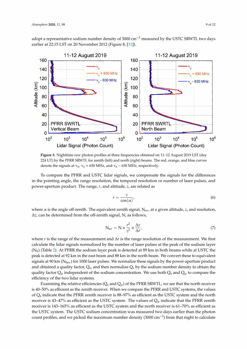
off-zenith to the north, both with a diameter of 0.91 m. The power aperture product of the lidar in bothdirections is 0.292 W-m2. The raw lidar signal measured by the PFRR SRWTL system at 23:44:20 LSTon 11 August 2019 (08:44:20, 12 August 2019 UT) represents the lidar signal acquired over 2 s (60 laserpulses) at each frequency at 30 m range resolution (Figure 5). We retrieved the sodium number densitywith 1 km zenith and 5 min temporal integration at 08:45 LST as 1780 cm−3 (zenith) and 1990 cm−3

(north). The north beam of the USTC lidar has a power of 780 mW, and the receiver telescope has adiameter of 0.76 m, pointing 30◦ off-zenith to the north [31]. The power aperture product is 0.354 W-m2.The east beam of the USTC lidar has a power of 520 mW, and the receiver telescope has a diameter of0.76 m, pointing 30◦ off-zenith to the east [31]. The power aperture product is 0.236 W-m2. We estimatethe raw lidar photon count signal measured by the east and north beams of the USTC SRWTL at 01:30LST on 23 November 2017 (17:30:13, 22 November 2017 UT) (Figure 5, [31]). These profiles representlidar signal acquired over 40 s (1200 laser pulses) for each frequency at 150 m range resolution. We

Atmosphere 2020, 11, 98 9 of 12

adopt a representative sodium number density of 3000 cm−3 measured by the USTC SRWTL two daysearlier at 22:15 LST on 20 November 2012 (Figure 8, [31]).Atmosphere 2020, 11, x FOR PEER REVIEW 9 of 12

Figure 5. Nighttime raw photon profiles at three frequencies obtained on 11–12 August 2019 LST (day 224 UT) by the PFRR SRWTL for zenith (left) and north (right) beams. The red, orange, and blue curves denote the signals at νa, νa + 630 MHz, and νa − 630 MHz, respectively.

To compare the PFRR and USTC lidar signals, we compensate the signals for the differences in the pointing angle, the range resolution, the temporal resolution or number of laser pulses, and power-aperture product. The range, r, and altitude, z, are related as

r = 𝑧 cos (α), (6)

where α is the angle off-zenith. The equivalent zenith signal, Nev, at a given altitude, z, and resolution, Δz, can be determined from the off-zenith signal, N, as follows, N = N , (7)

where r is the range of the measurement and Δr is the range resolution of the measurement. We first calculate the lidar signals normalized by the number of laser pulses at the peak of the sodium layer (NS) (Table 2). At PFRR the sodium layer peak is detected at 89 km in both beams while at USTC the peak is detected at 92 km in the east beam and 88 km in the north beam. We convert these to equivalent signals at 90 km (NSev) for 1000 laser pulses. We normalize these signals by the power-aperture product and obtained a quality factor, Qs, and then normalize Qs by the sodium number density to obtain the quality factor Qρ independent of the sodium concentration. We use both Qs and Qρ to compare the efficiency of the two lidar systems.

Table 2. Comparison PFRR SRWTL and University of Science and Technology of China (USTC) SRWTL.

Lidar System PA (W-m2) ρNa (cm−3) Nsig NBK NS NSev Qs Qρ PFRR SRWTL

Zenith 0.292 1780 3.1 × 101 1.1 × 10−1 5.1 × 10−1 17.4 60 33 North 0.292 1990 1.5 × 101 2.7 × 10−1 2.4 × 10−1 8.4 29 14

USTC SRWTL East 0.236 3000 3.0 × 103 3.7 × 101 2.5 × 100 16 68 23

North 0.354 3000 3.7 × 103 3.9 × 101 3.1 × 100 22 62 20

PA: power aperture product; ρNa: sodium number density, Nsig: lidar signal at the peak of the layer; NBK; background signal; NS: lidar signal per laser shot; NSev: equivalent zenith signal; QS: quality factor normalized by PA; Qρ: QS normalized by sodium concentration.

Figure 5. Nighttime raw photon profiles at three frequencies obtained on 11–12 August 2019 LST (day224 UT) by the PFRR SRWTL for zenith (left) and north (right) beams. The red, orange, and blue curvesdenote the signals at νa, νa + 630 MHz, and νa − 630 MHz, respectively.

To compare the PFRR and USTC lidar signals, we compensate the signals for the differencesin the pointing angle, the range resolution, the temporal resolution or number of laser pulses, andpower-aperture product. The range, r, and altitude, z, are related as

r =z

cos(α), (6)

where α is the angle off-zenith. The equivalent zenith signal, Nev, at a given altitude, z, and resolution,∆z, can be determined from the off-zenith signal, N, as follows,

Nev = N×r2

z2 ×∆z∆r

, (7)

where r is the range of the measurement and ∆r is the range resolution of the measurement. We firstcalculate the lidar signals normalized by the number of laser pulses at the peak of the sodium layer(NS) (Table 2). At PFRR the sodium layer peak is detected at 89 km in both beams while at USTC thepeak is detected at 92 km in the east beam and 88 km in the north beam. We convert these to equivalentsignals at 90 km (NSev) for 1000 laser pulses. We normalize these signals by the power-aperture productand obtained a quality factor, Qs, and then normalize Qs by the sodium number density to obtain thequality factor Qρ independent of the sodium concentration. We use both Qs and Qρ to compare theefficiency of the two lidar systems.

Examining the relative efficiencies (Qs and Qρ) of the PFRR SRWTL, we see that the north receiveris 40–50% as efficient as the zenith receiver. When we compare the PFRR and USTC systems, the valuesof Qs indicate that the PFRR zenith receiver is 88–97% as efficient as the USTC system and the northreceiver is 43–47% as efficient as the USTC system. The values of Qρ indicate that the PFRR zenithreceiver is 143–165% as efficient as the USTC system and the north receiver is 61–70% as efficient asthe USTC system. The USTC sodium concentration was measured two days earlier than the photoncount profiles, and we picked the maximum number density (3000 cm−3) from that night to calculate

Atmosphere 2020, 11, 98 10 of 12

Qρ. Thus, the Qρ we presented for the USTC system is a conservative value. Based on these analyses,we find that the zenith receiver of the PFRR lidar is operating with a slightly lower efficiency thanthe USTC system. This lower efficiency may be attributed to differences in the age of the detectorswhere the PFRR system has older PMTs than the USTC system. The lower efficiency of the PFRR northreceiver relative to the zenith receiver may be attributed to misalignment of the coupling fiber in thenorth receiver that requires further optimization.

Table 2. Comparison PFRR SRWTL and University of Science and Technology of China (USTC) SRWTL.

Lidar System PA (W-m2) ρNa (cm−3) Nsig NBK NS NSev Qs Qρ

PFRR SRWTLZenith 0.292 1780 3.1 × 101 1.1 × 10−1 5.1 × 10−1 17.4 60 33North 0.292 1990 1.5 × 101 2.7 × 10−1 2.4 × 10−1 8.4 29 14

USTC SRWTLEast 0.236 3000 3.0 × 103 3.7 × 101 2.5 × 100 16 68 23

North 0.354 3000 3.7 × 103 3.9 × 101 3.1 × 100 22 62 20

PA: power aperture product; ρNa: sodium number density, Nsig: lidar signal at the peak of the layer; NBK; backgroundsignal; NS: lidar signal per laser shot; NSev: equivalent zenith signal; QS: quality factor normalized by PA; Qρ: QSnormalized by sodium concentration.

5. Summary and Future Research

A sodium resonance wind-temperature lidar system has been deployed at PFRR. As the mostrecent deployment of this class of lidars, this system has the same architecture as the classic SRWTLbut incorporates a solid-state tunable diode laser as the seed laser that has been adopted by currentSRWTLs. This seed laser provides better stability, ease of use, and stable operation compared tothe ring dye lasers that were originally used in SRWTLs. The PFRR SRWTL lidar measures sodiumconcentration, wind, and temperature at the sodium layer altitude range (70–120 km). The transmitterof the system has been aligned and optimized to a level typical of other SRWTLs. However, moreeffort needs to be devoted to the alignment of the PDA in terms of the pumping efficiency to obtainmore output power (~20%). The receiver of the zenith telescope is optimized, while the receiver ofthe north telescope requires some further effort to improve the received signal (50%). An upgrade isin progress to add an eastward pointing beam and telescope. This upgrade will provide three-beammeasurements to the zenith, north, and east, and yield measurements of the complete wind vector.

Author Contributions: Investigation, J.L., B.P.W., J.H.A., and R.L.C.; supervision, R.L.C.; writing—original draft,J.L., B.P.W., and R.L.C. All authors have read and agreed to the published version of the manuscript.

Funding: This research was funded by the United States National Science Foundation under grants AGS-1829161,AGS-1829138, AGS-1734852, and AGS-1734693.

Acknowledgments: The authors acknowledge the staff at Poker Flat Research Range for the ongoing supportof the lidar program. The authors acknowledge Alan Liu, Tao Li, and Titus Yuan for helpful discussions. Theauthors acknowledge support for this research by the United States National Science Foundation under grantsAGS-1829161, AGS-1829138, AGS-1734852, and AGS-1734693.

Conflicts of Interest: The authors declare no conflict of interest.

References

1. Liu, H.L.; McInerney, J.M.; Santos, S.; Lauritzen, P.H.; Taylor, M.A.; Pedatella, N.M. Gravity waves simulatedby high-resolution Whole Atmosphere Community Climate Model. Geophys. Res. Lett. 2014, 41, 9106–9112.[CrossRef]

2. Yigit, E.; Koucká Knížová, P.; Georgieva, K.; Ward, W. A review of vertical coupling in theAtmosphere–Ionosphere system: Effects of waves, sudden stratospheric warmings, space weather, and ofsolar activity. J. Atmos. Sol. Terr. Phys. 2016, 141, 1–12. [CrossRef]

Atmosphere 2020, 11, 98 11 of 12

3. Jackson, D.R.; Fuller-Rowell, T.J.; Griffin, D.J.; Griffith, M.J.; Kelly, C.W.; Marsh, D.R.; Walach, M.T. FutureDirections for Whole Atmosphere Modeling: Developments in the Context of Space Weather. Space Weather2019, 17, 1342–1350. [CrossRef]

4. Gibson, A.J.; Thomas, L.; Bhattachacharyya, S.K. Laser observations of the ground-state hyperfine structureof sodium and of temperatures in the upper atmosphere. Nature 1979, 281, 131–132. [CrossRef]

5. Fricke, K.H.; von Zahn, U. Mesopause temperatures derived from probing the hyperfine structure of the D2resonance line of sodium by lidar. J. Atmos. Terr. Phys. 1985, 47, 499–512. [CrossRef]

6. She, C.Y.; Latifi, H.; Yu, J.R.; Alvarez Ii, R.J.; Bills, R.E.; Gardner, C.S. Two-frequency Lidar technique formesospheric Na temperature measurements. Geophys. Res. Lett. 1990, 17, 929–932. [CrossRef]

7. Bills, R.E.; Gardner, C.S.; Franke, S.J. Na Doppler/temperature lidar: Initial mesopause region observationsand comparison with the Urbana medium frequency radar. J. Geophys. Res. Atmos. 1991, 96, 22701–22707.[CrossRef]

8. Bills, R.E.; Gardner, C.S.; She, C.Y. Narrowband Lidar Technique for Sodium Temperature and Doppler WindObservations of the Upper Atmosphere; SPIE: Bellingham, WA, USA, 1991; Volume 30, pp. 13–21.

9. She, C.Y.; Yu, J.R.; Latifi, H.; Bills, R.E. High-spectral-resolution fluorescence light detection and ranging formesospheric sodium temperature measurements. Appl. Opt. 1992, 31, 2095–2106. [CrossRef]

10. She, C.Y.; Yu, J.R. Simultaneous three-frequency Na lidar measurements of radial wind and temperature inthe mesopause region. Geophys. Res. Lett. 1994, 21, 1771–1774. [CrossRef]

11. She, C.Y.; Li, T.; Collins, R.L.; Yuan, T.; Williams, B.P.; Kawahara, T.D.; Vance, J.D.; Acott, P.; Krueger, D.A.;Liu, H.L.; et al. Tidal perturbations and variability in the mesopause region over Fort Collins, CO (41N,105W): Continuous multi-day temperature and wind lidar observations. Geophys. Res. Lett. 2004, 31.[CrossRef]

12. Gardner, C.S.; Liu, A.Z. Seasonal variations of the vertical fluxes of heat and horizontal momentum in themesopause region at Starfire Optical Range, New Mexico. J. Geophys. Res. Atmos. (1984–2012) 2007, 112.[CrossRef]

13. Vance, J.D.; She, C.Y.; Moosmüller, H. Continuous-wave, all-solid-state, single-frequency 400-mW source at589 nm based on doubly resonant sum-frequency mixing in a monolithic lithium niobate resonator. Appl.Opt. 1998, 37, 4891–4896. [CrossRef]

14. Moosmuller, H.; Vance, J. Sum-frequency generation of continuous-wave sodium D-2 resonance radiation.Opt. Lett. 1997, 22, 1135–1137. [CrossRef] [PubMed]

15. Yue, J.; She, C.Y.; Williams, B.P.; Vance, J.D.; Acott, P.E.; Kawahara, T.D. Continuous-wave sodium D2resonance radiation generated in single-pass sum-frequency generation with periodically poled lithiumniobate. Opt. Lett. 2009, 34, 1093–1095. [CrossRef]

16. She, C.Y.; Vance, J.D.; Williams, B.P.; Krueger, D.A.; Moosmüller, H.; Gibson-Wilde, D.; Fritts, D. Lidar studiesof atmospheric dynamics near polar mesopause. Eos Trans. Am. Geophys. Union 2002, 83. [CrossRef]

17. Williams, B.P.; Fritts, D.C.; Wang, L.; She, C.Y.; Vance, J.D.; Schmidlin, F.J.; Goldberg, R.A.; Müllemann, A.;Lübken, F.J. Gravity waves in the arctic mesosphere during the MaCWAVE/MIDAS summer rocket program.Geophys. Res. Lett. 2004, 31. [CrossRef]

18. Eismann, U.; Enderlein, M.; Simeonidis, K.; Keller, F.; Rohde, F.; Opalevs, D.; Scholz, M.; Kaenders, W.;Stuhler, J. Active and passive stabilization of a high-power violet frequency-doubled diode laser. InProceedings of the Conference on Lasers and Electro-Optics, San Jose, CA, USA, 5 June 2016; p. JTu5A.65.

19. Liu, A.Z.; Guo, Y.; Vargas, F.; Swenson, G.R. First measurement of horizontal wind and temperature in thelower thermosphere (105–140 km) with a Na Lidar at Andes Lidar Observatory. Geophys. Res. Lett. 2016, 43,2374–2380. [CrossRef]

20. Guo, Y.; Liu, A.Z.; Gardner, C.S. First Na lidar measurements of turbulence heat flux, thermal diffusivity, andenergy dissipation rate in the mesopause region. Geophys. Res. Lett. 2017, 44, 5782–5790. [CrossRef]

21. Gardner, C.S. Performance capabilities of middle-atmosphere temperature lidars: Comparison of Na, Fe, K,Ca, Ca+, and Rayleigh systems. Appl. Opt. 2004, 43, 4941–4956. [CrossRef]

22. She, C.Y.; Yu, J.R. Doppler-free saturation fluorescence spectroscopy of Na atoms for atmospheric application.Appl. Opt. 1995, 34, 1063–1075. [CrossRef]

23. Chu, X.; Papen, G.C. Resonance fluorescence lidar for measurements of the middle and upper atmosphere.In Laser Remote Sensing; Fujii, T., Fukuchi, T., Eds.; CRC Press: Boca Raton, FL, USA, 2005.

Atmosphere 2020, 11, 98 12 of 12

24. Krueger, D.A.; She, C.Y.; Yuan, T. Retrieving mesopause temperature and line-of-sight wind fromfull-diurnal-cycle Na lidar observations. Appl. Opt. 2015, 54, 9469. [CrossRef] [PubMed]

25. Harrell, S.D.; She, C.-Y.; Yuan, T.; Krueger, D.A.; Chen, H.; Chen, S.S.; Hu, Z.L. Sodium and potassium vaporFaraday filters revisited: theory and applications. J. Opt. Soc. Am. B 2009, 26, 659–670. [CrossRef]

26. White, M.A. A Frequency-Agile Na Lidar for the Measurement of Temperature and Velocity in the MesopauseRegion. Ph.D. Thesis, Colorado State University, Fort Collins, CO, USA, 1999.

27. Acott, P.E. Mesospheric Momentum Flux Studies over Fort Collins CO (41N, 105W); Colorado State University:Fort Collins, CO, USA, 2009.

28. Vance, J.D. The Sum Frequency Generator Seeded, ALOMAR Weber Sodium LIDAR and Initial Measurementsof Temperature and Wind in the Norwegian Arctic Mesopause Region. Ph.D. Thesis, Colorado State University,Fort Collins, CO, USA, 2004.

29. Titus, T.; (Utah State University, Logan, UT, USA). Personal communication, 2019.30. Liu, A.Z.; (Embry-Riddle Aeronautical University, Daytona Beach, FL, USA). Personal communication, 2019.31. Li, T.; Fang, X.; Liu, W.; Gu, S.Y.; Dou, X. Narrowband sodium lidar for the measurements of mesopause

region temperature and wind. Appl. Opt. 2012, 51, 5401–5411. [CrossRef] [PubMed]32. Papoulis, A.; Pillai, S.U. Probability, Random Variables and Stochastic Processes, 4th ed.; The McGraw-Hill

Companies: New York, NY, USA, 2002.33. Su, L.; Collins, R.L.; Krueger, D.A.; She, C.Y. Statistical Analysis of Sodium Doppler Wind–Temperature

Lidar Measurements of Vertical Heat Flux. J. Atmos. Ocean. Technol. 2008, 25, 401–415. [CrossRef]

© 2020 by the authors. Licensee MDPI, Basel, Switzerland. This article is an open accessarticle distributed under the terms and conditions of the Creative Commons Attribution(CC BY) license (http://creativecommons.org/licenses/by/4.0/).