social data science - tidy data, data manipulation & … · mystique bad female marvel batman...
TRANSCRIPT
social data scienceTidy Data, Data Manipulation & Functions
Sebastian BarfortAugust 08, 2016
University of CopenhagenDepartment of Economics
1/107

intro
“Herein lies the dirty secret about most data scientists’ work– it’s more data munging than deep learning. The bestminds of my generation are deleting commas from log files,and that makes me sad. A Ph.D. is a terrible thing to waste.”
Source
2/107

data janitor
Source
3/107
raw versus processed data
Raw data
The original source of the data
Often hard to use directly for data analysis
You should never process your original data
Processed data
Data that is ready for analysis
Data manipulation involves going from raw to processed data.
This can include merging, subsetting, transforming, etc.
All steps that take you from raw to processed data should be scripted
4/107

today
Introduce some tricks for working (efficiently) with data
Introduce concept and tools for working with tidy data (tidyr)Manipulate tidy data using dplyrIterate over elements using functions (purrr)String processing (stringr, regular expressions)
5/107
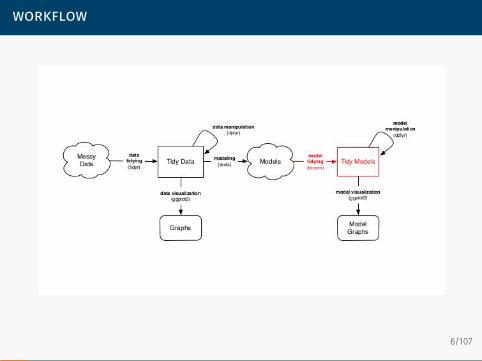
workflow
6/107

The Pipe
7/107

digression: the pipe
8/107

the pipe operator
The pipe operator %>% (RStudio has keyboard shortcuts, learn to usethem!) let’s you write sequences instead of nested functions
x %>% f(y) -> f(x,y)x %>% f(z, .) -> f(z, x)Read %>% as “then”. First do this, then do this, etc…It’s implemented in R by a Danish econometricianAll the packages you will learn today work with the pipe.
9/107


Tidy data
11/107

tidyr
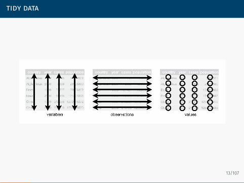
Tidy data: observations are in the rows, variables are in the columns
tidyr: take your messy data and turn it into a tidy formatAdvantages of tidy data:
· Consistency· Allows you to spend more time on your analysis· Speed
12/107
tidy data
13/107

functions in tidyr
· gather: Reshape from wide to long· spread: Reshape from long to wide· separate: Split a variable into multiple variables.
(Also more complicated functions such as nest for nested dataframes, but we won’t go into detail with those here)
14/107

read data
library(”readr”)gh.link = ”https://raw.githubusercontent.com/”user.repo = ”hadley/tidyr/”branch = ”master/”link = ”vignettes/pew.csv”data.link = paste0(gh.link, user.repo, branch, link)df = read_csv(data.link)
15/107

pew data
First five columns
religion <$10k $10-20k $20-30k $30-40k
Agnostic 27 34 60 81Atheist 12 27 37 52Buddhist 27 21 30 34
Question 1: What variables are in this dataset?
Question 2: How does a tidy version of this data look like?
16/107
the gather function
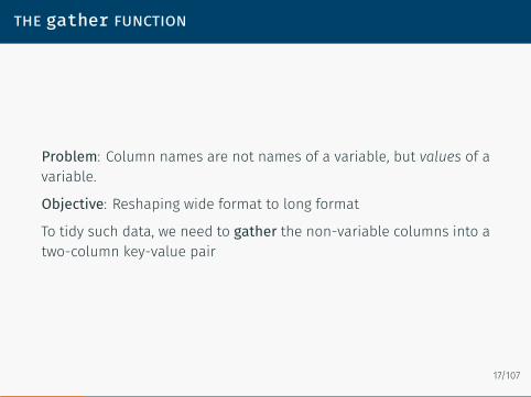
Problem: Column names are not names of a variable, but values of avariable.
Objective: Reshaping wide format to long format
To tidy such data, we need to gather the non-variable columns into atwo-column key-value pair
17/107
gather
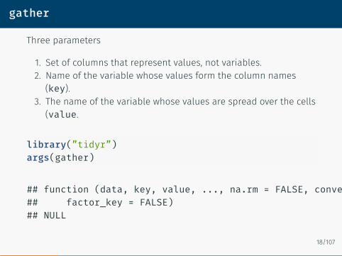
Three parameters
1. Set of columns that represent values, not variables.2. Name of the variable whose values form the column names(key).
3. The name of the variable whose values are spread over the cells(value.
library(”tidyr”)args(gather)
## function (data, key, value, ..., na.rm = FALSE, convert = FALSE,## factor_key = FALSE)## NULL
18/107

gather pew data
df.gather = df %>%gather(key = income,
value = frequency,-religion)
19/107
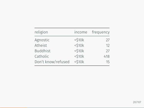
religion income frequency
Agnostic <$10k 27Atheist <$10k 12Buddhist <$10k 27Catholic <$10k 418Don’t know/refused <$10k 15
20/107

alternatives
This
df %>%gather(key = income,
value = frequency,2:11)
returns the same as
df %>%gather(key = income,
value = frequency,-religion)
21/107
more complicated example
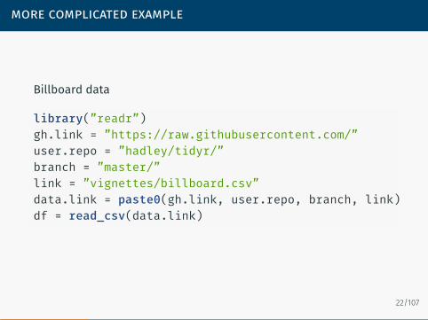
Billboard data
library(”readr”)gh.link = ”https://raw.githubusercontent.com/”user.repo = ”hadley/tidyr/”branch = ”master/”link = ”vignettes/billboard.csv”data.link = paste0(gh.link, user.repo, branch, link)df = read_csv(data.link)
22/107
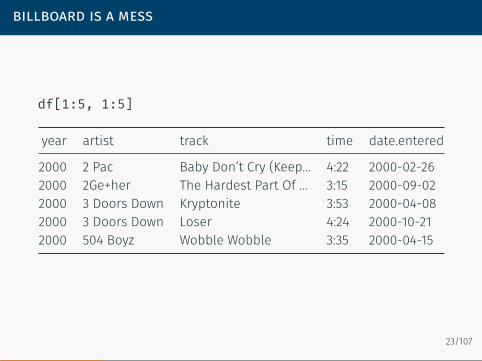
billboard is a mess
df[1:5, 1:5]
year artist track time date.entered
2000 2 Pac Baby Don’t Cry (Keep… 4:22 2000-02-262000 2Ge+her The Hardest Part Of … 3:15 2000-09-022000 3 Doors Down Kryptonite 3:53 2000-04-082000 3 Doors Down Loser 4:24 2000-10-212000 504 Boyz Wobble Wobble 3:35 2000-04-15
23/107
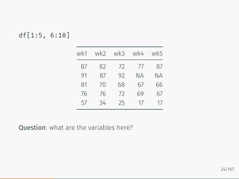
df[1:5, 6:10]
wk1 wk2 wk3 wk4 wk5
87 82 72 77 8791 87 92 NA NA81 70 68 67 6676 76 72 69 6757 34 25 17 17
Question: what are the variables here?
24/107
tidying the billboard data
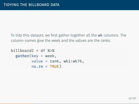
To tidy this dataset, we first gather together all the wk columns. Thecolumn names give the week and the values are the ranks:
billboard2 = df %>%gather(key = week,
value = rank, wk1:wk76,na.rm = TRUE)
25/107

Not displaying the track column
year artist time date.entered week rank
2000 2 Pac 4:22 2000-02-26 wk1 872000 2Ge+her 3:15 2000-09-02 wk1 912000 3 Doors Down 3:53 2000-04-08 wk1 812000 3 Doors Down 4:24 2000-10-21 wk1 762000 504 Boyz 3:35 2000-04-15 wk1 57
Are we done?
26/107
data cleaning
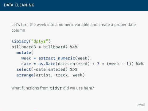
Let’s turn the week into a numeric variable and create a proper datecolumn
library(”dplyr”)billboard3 = billboard2 %>%mutate(
week = extract_numeric(week),date = as.Date(date.entered) + 7 * (week - 1)) %>%
select(-date.entered) %>%arrange(artist, track, week)
What functions from tidyr did we use here?
27/107

year artist track time week
2000 2 Pac Baby Don’t Cry (Keep… 4:22 12000 2 Pac Baby Don’t Cry (Keep… 4:22 22000 2 Pac Baby Don’t Cry (Keep… 4:22 32000 2 Pac Baby Don’t Cry (Keep… 4:22 42000 2 Pac Baby Don’t Cry (Keep… 4:22 5
28/107
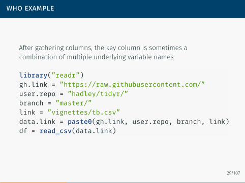
who example
After gathering columns, the key column is sometimes acombination of multiple underlying variable names.
library(”readr”)gh.link = ”https://raw.githubusercontent.com/”user.repo = ”hadley/tidyr/”branch = ”master/”link = ”vignettes/tb.csv”data.link = paste0(gh.link, user.repo, branch, link)df = read_csv(data.link)
29/107
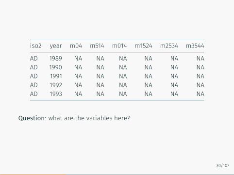
iso2 year m04 m514 m014 m1524 m2534 m3544
AD 1989 NA NA NA NA NA NAAD 1990 NA NA NA NA NA NAAD 1991 NA NA NA NA NA NAAD 1992 NA NA NA NA NA NAAD 1993 NA NA NA NA NA NA
Question: what are the variables here?
30/107

answer
The dataset comes from the World Health Organisation, and recordsthe counts of confirmed tuberculosis cases by country, year, anddemographic group. The demographic groups are broken down bysex (m, f) and age (0-14, 15-25, 25-34, 35-44, 45-54, 55-64, unknown).
31/107
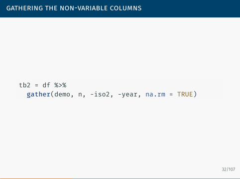
gathering the non-variable columns
tb2 = df %>%gather(demo, n, -iso2, -year, na.rm = TRUE)
32/107
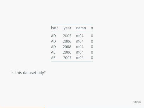
iso2 year demo n
AD 2005 m04 0AD 2006 m04 0AD 2008 m04 0AE 2006 m04 0AE 2007 m04 0
Is this dataset tidy?
33/107
separating the demo variable
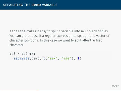
separate makes it easy to split a variable into multiple variables.You can either pass it a regular expression to split on or a vector ofcharacter positions. In this case we want to split after the firstcharacter.
tb3 = tb2 %>%separate(demo, c(”sex”, ”age”), 1)
34/107

iso2 year sex age n
AD 2005 m 04 0AD 2006 m 04 0AD 2008 m 04 0AE 2006 m 04 0AE 2007 m 04 0
35/107
reshaping from long to wide format
There are times when we are required to turn long formatted datainto wide formatted data. The spread function spreads a key-valuepair across multiple columns.
36/107
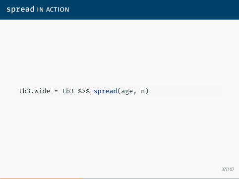
spread in action
tb3.wide = tb3 %>% spread(age, n)
37/107

iso2 year sex 014 04 1524 2534 3544
AD 1996 f 0 NA 1 1 0AD 1996 m 0 NA 0 0 4AD 1997 f 0 NA 1 2 3AD 1997 m 0 NA 0 1 2AD 1998 m 0 NA 0 0 1
38/107
Data Manipulation
39/107
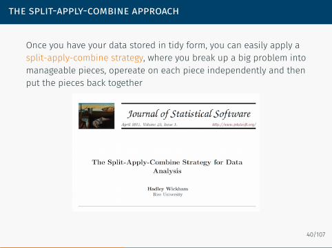
the split-apply-combine approach
Once you have your data stored in tidy form, you can easily apply asplit-apply-combine strategy, where you break up a big problem intomanageable pieces, opereate on each piece independently and thenput the pieces back together
40/107

split-apply-combine
41/107

the dplyr package
dplyr: (efficiently) split-apply-combine for data framesVerbs a verb is a function that takes a data frame as it’s firstargument
· filter: select rows· arrange: order rows· select: select columns· rename: rename columns· distinct: find distinct rows· mutate: add new variables· summarise: summarize across a data set· sample_n: sample from a data set
42/107
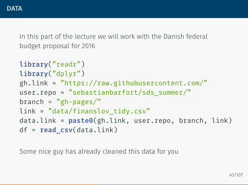
data
In this part of the lecture we will work with the Danish federalbudget proposal for 2016
library(”readr”)library(”dplyr”)gh.link = ”https://raw.githubusercontent.com/”user.repo = ”sebastianbarfort/sds_summer/”branch = ”gh-pages/”link = ”data/finanslov_tidy.csv”data.link = paste0(gh.link, user.repo, branch, link)df = read_csv(data.link)
Some nice guy has already cleaned this data for you
43/107
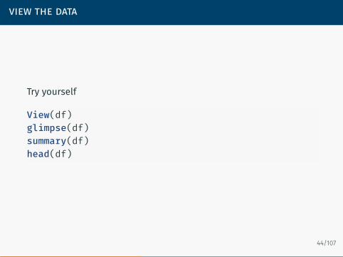
view the data
Try yourself
View(df)glimpse(df)summary(df)head(df)
44/107
filtering data i
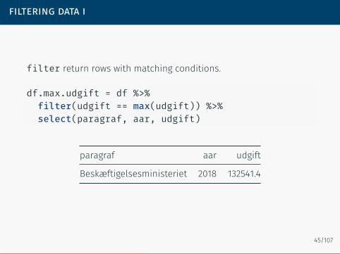
filter return rows with matching conditions.
df.max.udgift = df %>%filter(udgift == max(udgift)) %>%select(paragraf, aar, udgift)
paragraf aar udgift
Beskæftigelsesministeriet 2018 132541.4
45/107
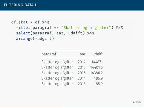
filtering data ii
df.skat = df %>%filter(paragraf == ”Skatter og afgifter”) %>%select(paragraf, aar, udgift) %>%arrange(-udgift)
paragraf aar udgift
Skatter og afgifter 2014 14487.1Skatter og afgifter 2015 14401.6Skatter og afgifter 2016 14386.2Skatter og afgifter 2014 185.9Skatter og afgifter 2015 185.9
46/107

logical operators
47/107
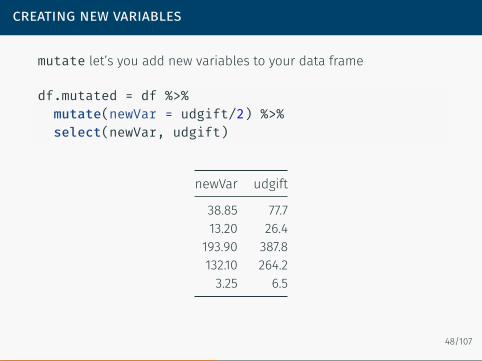
creating new variables
mutate let’s you add new variables to your data frame
df.mutated = df %>%mutate(newVar = udgift/2) %>%select(newVar, udgift)
newVar udgift
38.85 77.713.20 26.4193.90 387.8132.10 264.23.25 6.5
48/107

sampling from a data frame
We can sample from a data frame using sample_n andsample_frac
df.sample.n = df %>%select(paragraf, aar, udgift) %>%sample_n(3)
paragraf aar udgift
Erhvervs- og Vækstministeriet 2017 -26.0Transport- og Bygningsministeriet 2016 5.4Beskæftigelsesministeriet 2016 0.6
49/107

grouped operations
So far, we have primarily learned how to manipulate data frames.
The dplyr package becomes really powerful when we introduce thegroup_by functiongroup_by breaks down a dataset into specified groups of rows.When you then apply the verbs above on the resulting object they’llbe automatically applied “by group”.
Use in conjunction with mutate (to add existing rows to your dataframe) or summarise (to create a new data frame)
50/107

common mutate/summarise options
· mean: mean within groups· sum: sum within groups· sd: standard deviation within groups· max: max within groups· n(): number in each group· first: first in group· last: last in group· nth(n = 3): nth in group (3rd here)· tally: count number in group
51/107

operating on groups i
Which ministry has the largest expenses?
df.expense = df %>%group_by(paragraf) %>%summarise(sum.exp = sum(udgift, na.rm = TRUE)) %>%arrange(-sum.exp)
paragraf sum.exp
Social- og Indenrigsministeriet 1231214.6Beskæftigelsesministeriet 1146997.8Uddannelses- og Forskningsministeriet 296539.2Min. for Børn, Undervisning og Ligestilling 180955.1Pensionsvæsenet 139058.0
52/107
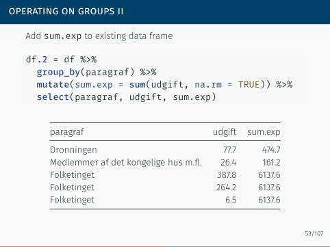
operating on groups ii
Add sum.exp to existing data frame
df.2 = df %>%group_by(paragraf) %>%mutate(sum.exp = sum(udgift, na.rm = TRUE)) %>%select(paragraf, udgift, sum.exp)
paragraf udgift sum.exp
Dronningen 77.7 474.7Medlemmer af det kongelige hus m.fl. 26.4 161.2Folketinget 387.8 6137.6Folketinget 264.2 6137.6Folketinget 6.5 6137.6
53/107

operating on groups iii
You can group by several variables
df.expense.2 = df %>%group_by(paragraf, aar) %>%summarise(sum.exp = sum(udgift, na.rm = TRUE)) %>%arrange(sum.exp)
paragraf aar sum.exp
Afdrag på statsgælden (netto) 2016 -77832.3Afdrag på statsgælden (netto) 2015 -32519.9Afdrag på statsgælden (netto) 2017 0.0Afdrag på statsgælden (netto) 2018 0.0Afdrag på statsgælden (netto) 2019 0.0
54/107
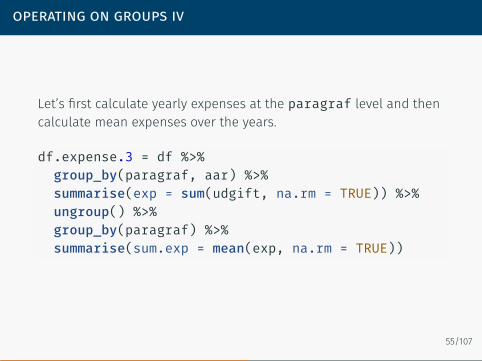
operating on groups iv
Let’s first calculate yearly expenses at the paragraf level and thencalculate mean expenses over the years.
df.expense.3 = df %>%group_by(paragraf, aar) %>%summarise(exp = sum(udgift, na.rm = TRUE)) %>%ungroup() %>%group_by(paragraf) %>%summarise(sum.exp = mean(exp, na.rm = TRUE))
55/107

paragraf sum.exp
Afdrag på statsgælden (netto) -14628.13333Beholdningsbevægelser mv. 1540.65000Beskæftigelsesministeriet 191166.30000Dronningen 79.11667Energi-, Forsynings- og Klimaministeriet 2433.18333
56/107

merging data sets
57/107
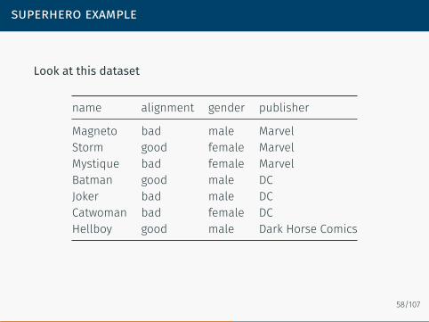
superhero example
Look at this dataset
name alignment gender publisher
Magneto bad male MarvelStorm good female MarvelMystique bad female MarvelBatman good male DCJoker bad male DCCatwoman bad female DCHellboy good male Dark Horse Comics
58/107

publishers
And this
publisher yr_founded
DC 1934Marvel 1939Image 1992
59/107
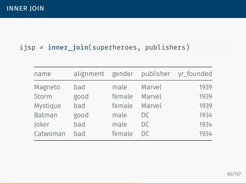
inner join
ijsp = inner_join(superheroes, publishers)
name alignment gender publisher yr_founded
Magneto bad male Marvel 1939Storm good female Marvel 1939Mystique bad female Marvel 1939Batman good male DC 1934Joker bad male DC 1934Catwoman bad female DC 1934
60/107

left join
ljsp = left_join(superheroes, publishers)
name alignment gender publisher yr_founded
Magneto bad male Marvel 1939Storm good female Marvel 1939Mystique bad female Marvel 1939Batman good male DC 1934Joker bad male DC 1934Catwoman bad female DC 1934Hellboy good male Dark Horse Comics NA
61/107

merging different names
superheroes = superheroes %>%mutate(seblikes = (publisher == ”Marvel”))
publishers = publishers %>%mutate(seb = (publisher == ”Marvel”))
ij2 = inner_join(superheroes,publishers)
## Joining by: ”publisher”
62/107

name alignment gender publisher seblikes yr_founded seb
Magneto bad male Marvel TRUE 1939 TRUEStorm good female Marvel TRUE 1939 TRUEMystique bad female Marvel TRUE 1939 TRUEBatman good male DC FALSE 1934 FALSEJoker bad male DC FALSE 1934 FALSECatwoman bad female DC FALSE 1934 FALSE
63/107
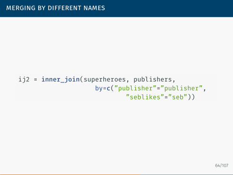
merging by different names
ij2 = inner_join(superheroes, publishers,by=c(”publisher”=”publisher”,
”seblikes”=”seb”))
64/107
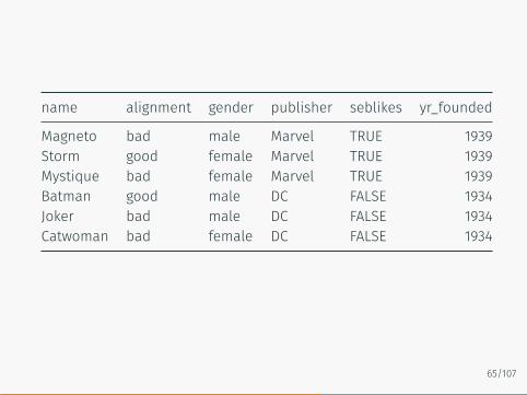
name alignment gender publisher seblikes yr_founded
Magneto bad male Marvel TRUE 1939Storm good female Marvel TRUE 1939Mystique bad female Marvel TRUE 1939Batman good male DC FALSE 1934Joker bad male DC FALSE 1934Catwoman bad female DC FALSE 1934
65/107
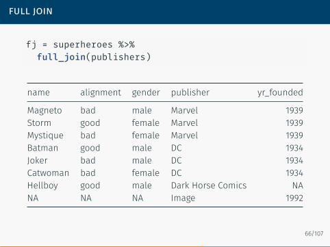
full join
fj = superheroes %>%full_join(publishers)
name alignment gender publisher yr_founded
Magneto bad male Marvel 1939Storm good female Marvel 1939Mystique bad female Marvel 1939Batman good male DC 1934Joker bad male DC 1934Catwoman bad female DC 1934Hellboy good male Dark Horse Comics NANA NA NA Image 1992
66/107

Functions and Iteration
67/107
introduction
Perhaps most important skill for being effective when working withdata: write functions.
Advantages
1. You drastically reduce risk of making mistakes2. When something exogenous changes, you only need to updatecode in one place
3. You can give your function an intuitive name that makes yourcode easier to read
You should write functions to increase your productivity.
68/107
69/107
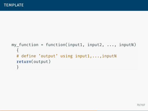
template
my_function = function(input1, input2, ..., inputN){# define ’output’ using input1,...,inputNreturn(output)}
70/107
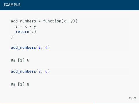
example
add_numbers = function(x, y){z = x + yreturn(z)
}
add_numbers(2, 4)
## [1] 6
add_numbers(2, 6)
## [1] 8
71/107
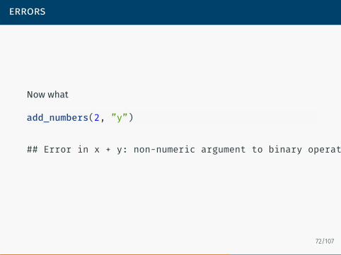
errors
Now what
add_numbers(2, ”y”)
## Error in x + y: non-numeric argument to binary operator
72/107
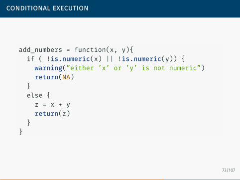
conditional execution
add_numbers = function(x, y){if ( !is.numeric(x) || !is.numeric(y)) {
warning(”either ’x’ or ’y’ is not numeric”)return(NA)
}else {
z = x + yreturn(z)
}}
73/107

testing
add_numbers(2, 4)
## [1] 6
add_numbers(2, ”y”)
## Warning in add_numbers(2, ”y”): either ’x’ or ’y’ is not numeric
## [1] NA
74/107
iteration
One important skill for being an effective data analyst was beingable to write functions. A second is iteration.
Iteration helps you when you need to do the same thing to multipleinputs. For example, repeating the same function on lots of inputs.
Two iteration paradigms
1. Imperative programming (for loops, etc.)2. Functional programming
75/107
data
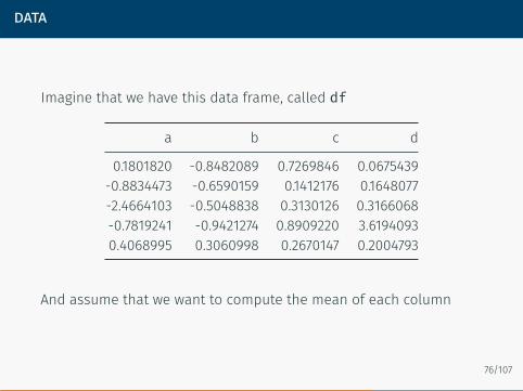
Imagine that we have this data frame, called df
a b c d
0.1801820 -0.8482089 0.7269846 0.0675439-0.8834473 -0.6590159 0.1412176 0.1648077-2.4664103 -0.5048838 0.3130126 0.3166068-0.7819241 -0.9421274 0.8909220 3.61940930.4068995 0.3060998 0.2670147 0.2004793
And assume that we want to compute the mean of each column
76/107
the for loop
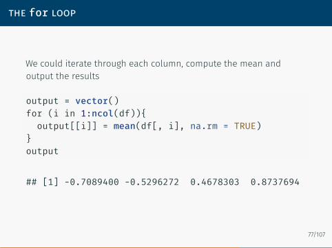
We could iterate through each column, compute the mean andoutput the results
output = vector()for (i in 1:ncol(df)){output[[i]] = mean(df[, i], na.rm = TRUE)
}output
## [1] -0.7089400 -0.5296272 0.4678303 0.8737694
77/107
your turn
We will do Exercise 4.5.1 in Imai (2016).
78/107

read data
intrade
library(”readr”)gh.link = ”https://raw.githubusercontent.com/”user.repo = ”kosukeimai/qss/”branch = ”master/”link = ”PREDICTION/intrade08.csv”data.link = paste0(gh.link, user.repo, branch, link)intrade.08 = read_csv(data.link)
link = ”PREDICTION/intrade12.csv”data.link = paste0(gh.link, user.repo, branch, link)intrade.12 = read_csv(data.link)
79/107

Name Description
day Date of the sessionstatename Full name of each statestate Abbreviation of each statePriceD Predicted vote share of D Nominee’s marketPriceR Predicted vote share of R Nominee’s marketVolumeD Total session trades of D Nominee’s marketVolumeR Total session trades of R Nominee’s market
80/107
pres
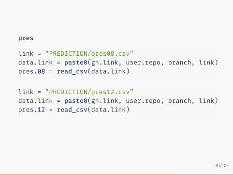
link = ”PREDICTION/pres08.csv”data.link = paste0(gh.link, user.repo, branch, link)pres.08 = read_csv(data.link)
link = ”PREDICTION/pres12.csv”data.link = paste0(gh.link, user.repo, branch, link)pres.12 = read_csv(data.link)
81/107

Name Description
state.name Full name of state (only in pres2008)state Two letter state abbreviationObama Vote percentage for ObamaMcCain Vote percentage for McCainEV Number of electoral college votes for this state
82/107
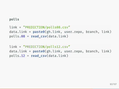
polls
link = ”PREDICTION/polls08.csv”data.link = paste0(gh.link, user.repo, branch, link)polls.08 = read_csv(data.link)
link = ”PREDICTION/polls12.csv”data.link = paste0(gh.link, user.repo, branch, link)polls.12 = read_csv(data.link)
83/107

Name Description
state Abbreviated name of state in which poll was conductedObama Predicted support for Obama (percentage)Romney Predicted support for Romney (percentage)Pollster Name of organization conducting pollmiddate Middle of the period when poll was conducted
84/107
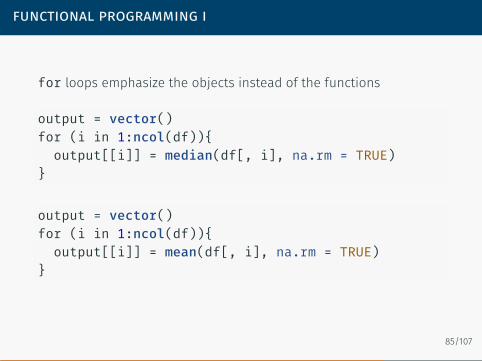
functional programming i
for loops emphasize the objects instead of the functions
output = vector()for (i in 1:ncol(df)){output[[i]] = median(df[, i], na.rm = TRUE)
}
output = vector()for (i in 1:ncol(df)){output[[i]] = mean(df[, i], na.rm = TRUE)
}
85/107

functional programming ii
library(”purrr”)map_dbl(df, mean)
## a b c d## -0.7089400 -0.5296272 0.4678303 0.8737694
map_dbl(df, median)
## a b c d## -0.7819241 -0.6590159 0.3130126 0.2004793
86/107

using you own function
my_function = function(df){my.mean = mean(df, na.rm = TRUE)my.string = paste(”mean is”,
round(my.mean, 2),sep = ”:”)
return(my.string)}
map_chr(df, my_function)
## a b c d## ”mean is:-0.71” ”mean is:-0.53” ”mean is:0.47” ”mean is:0.87”
87/107
String Processing
88/107
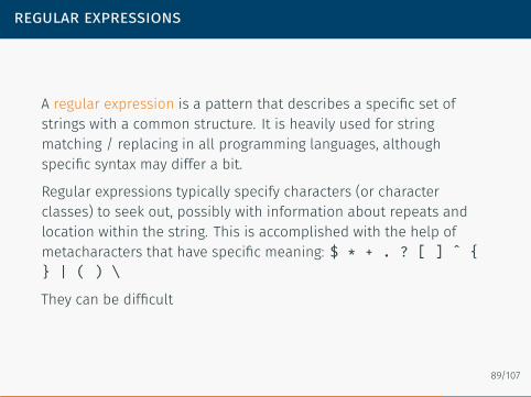
regular expressions
A regular expression is a pattern that describes a specific set ofstrings with a common structure. It is heavily used for stringmatching / replacing in all programming languages, althoughspecific syntax may differ a bit.
Regular expressions typically specify characters (or characterclasses) to seek out, possibly with information about repeats andlocation within the string. This is accomplished with the help ofmetacharacters that have specific meaning: $ * + . ? [ ] ˆ {} | ( ) \They can be difficult
89/107

90/107
quantifiers
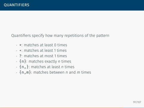
Quantifiers specify how many repetitions of the pattern
· *: matches at least 0 times· +: matches at least 1 times· ?: matches at most 1 times· {n}: matches exactly n times· {n,}: matches at least n times· {n,m}: matches between n and m times
91/107
example
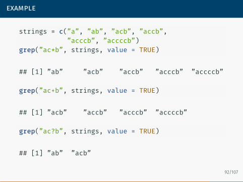
strings = c(”a”, ”ab”, ”acb”, ”accb”,”acccb”, ”accccb”)
grep(”ac*b”, strings, value = TRUE)
## [1] ”ab” ”acb” ”accb” ”acccb” ”accccb”
grep(”ac+b”, strings, value = TRUE)
## [1] ”acb” ”accb” ”acccb” ”accccb”
grep(”ac?b”, strings, value = TRUE)
## [1] ”ab” ”acb”
92/107
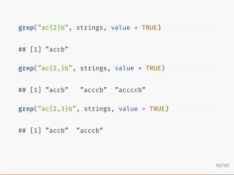
grep(”ac{2}b”, strings, value = TRUE)
## [1] ”accb”
grep(”ac{2,}b”, strings, value = TRUE)
## [1] ”accb” ”acccb” ”accccb”
grep(”ac{2,3}b”, strings, value = TRUE)
## [1] ”accb” ”acccb”
93/107
operators
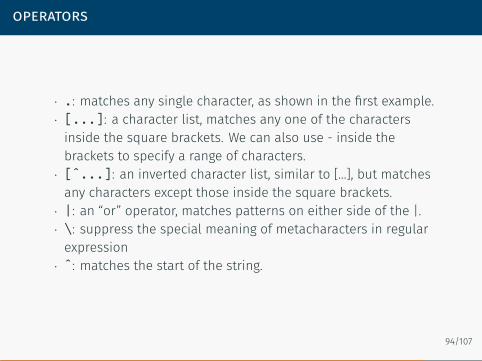
· .: matches any single character, as shown in the first example.· [...]: a character list, matches any one of the charactersinside the square brackets. We can also use - inside thebrackets to specify a range of characters.
· [ˆ...]: an inverted character list, similar to […], but matchesany characters except those inside the square brackets.
· |: an “or” operator, matches patterns on either side of the |.· \: suppress the special meaning of metacharacters in regularexpression
· ˆ: matches the start of the string.
94/107

example
strings = c(”^ab”, ”ab”, ”abc”, ”abd”, ”abe”, ”ab 12”)grep(”ab.”, strings, value = TRUE)
## [1] ”abc” ”abd” ”abe” ”ab 12”
grep(”ab[c-e]”, strings, value = TRUE)
## [1] ”abc” ”abd” ”abe”
grep(”ab[^c]”, strings, value = TRUE)
## [1] ”abd” ”abe” ”ab 12”
95/107
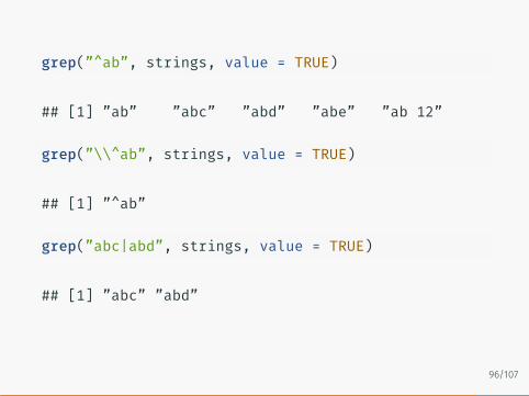
grep(”^ab”, strings, value = TRUE)
## [1] ”ab” ”abc” ”abd” ”abe” ”ab 12”
grep(”\\^ab”, strings, value = TRUE)
## [1] ”^ab”
grep(”abc|abd”, strings, value = TRUE)
## [1] ”abc” ”abd”
96/107
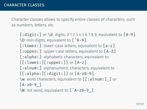
character classes
Character classes allows to specify entire classes of characters, suchas numbers, letters, etc.
· [:digit:] or \d: digits, 0 1 2 3 4 5 6 7 8 9, equivalent to [0-9].· \D: non-digits, equivalent to [ˆ0-9].· [:lower:]: lower-case letters, equivalent to [a-z].· [:upper:]: upper-case letters, equivalent to [A-Z].· [:alpha:]: alphabetic characters, equivalent to[[:lower:][:upper:]] or [A-z].
· [:alnum:]: alphanumeric characters, equivalent to[[:alpha:][:digit:]] or [A-z0-9].
· \w: word characters, equivalent to [[:alnum:]_] or[A-z0-9_].
· \W: not word, equivalent to [ˆA-z0-9_].
97/107
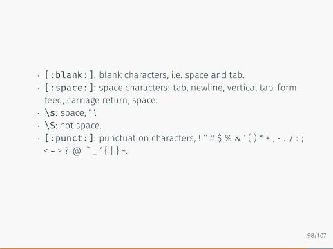
· [:blank:]: blank characters, i.e. space and tab.· [:space:]: space characters: tab, newline, vertical tab, formfeed, carriage return, space.
· \s: space, ‘ ‘.· \S: not space.· [:punct:]: punctuation characters, ! ” # $ % & ’ ( ) * + , - . / : ;< = > ? @ ˆ _ ‘ { | } ~.
98/107
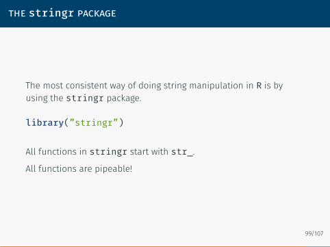
the stringr package
The most consistent way of doing string manipulation in R is byusing the stringr package.
library(”stringr”)
All functions in stringr start with str_.All functions are pipeable!
99/107
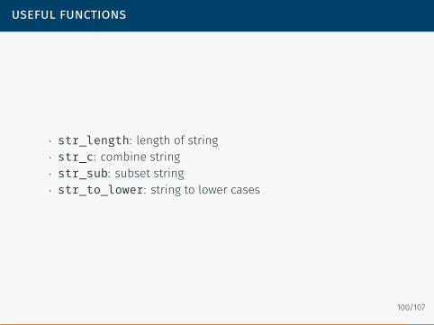
useful functions
· str_length: length of string· str_c: combine string· str_sub: subset string· str_to_lower: string to lower cases
100/107

matching with regular expressions
Detect matches
x = c(”apple”, ”banana”, ”pear”, ”213”)x %>% str_detect(”e”)
## [1] TRUE FALSE TRUE FALSE
x %>% str_detect(”[0-9]”)
## [1] FALSE FALSE FALSE TRUE
x %>% str_detect(”e.r”)
## [1] FALSE FALSE TRUE FALSE101/107
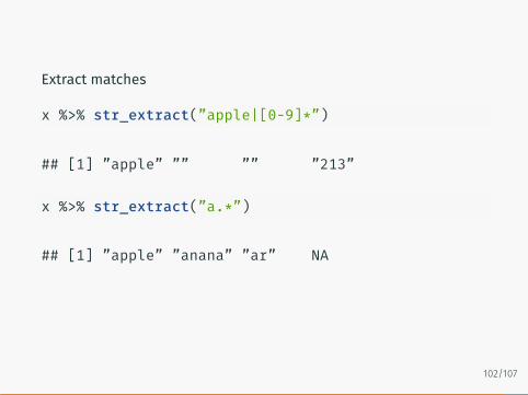
Extract matches
x %>% str_extract(”apple|[0-9]*”)
## [1] ”apple” ”” ”” ”213”
x %>% str_extract(”a.*”)
## [1] ”apple” ”anana” ”ar” NA
102/107
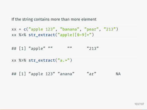
If the string contains more than more element
xx = c(”apple 123”, ”banana”, ”pear”, ”213”)xx %>% str_extract(”apple|[0-9]*”)
## [1] ”apple” ”” ”” ”213”
xx %>% str_extract(”a.*”)
## [1] ”apple 123” ”anana” ”ar” NA
103/107

xx %>% str_extract_all(”apple|[0-9].”)
## [[1]]## [1] ”apple” ”12”#### [[2]]## character(0)#### [[3]]## character(0)#### [[4]]## [1] ”21”
104/107

replacing
Replacing
xx %>% str_replace(”[0-9]”, ”\\?”)
## [1] ”apple ?23” ”banana” ”pear” ”?13”
xx %>% str_replace_all(”[0-9]”, ”\\?”)
## [1] ”apple ???” ”banana” ”pear” ”???”
xx %>% str_replace_all(c(”1” = ”one”, ”2” = ”x”))
## [1] ”apple onex3” ”banana” ”pear” ”xone3”
105/107
split vector
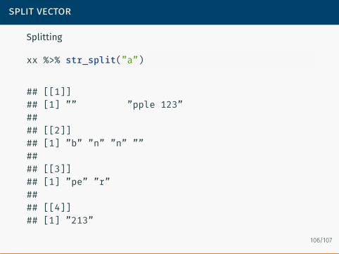
Splitting
xx %>% str_split(”a”)
## [[1]]## [1] ”” ”pple 123”#### [[2]]## [1] ”b” ”n” ”n” ””#### [[3]]## [1] ”pe” ”r”#### [[4]]## [1] ”213”
106/107
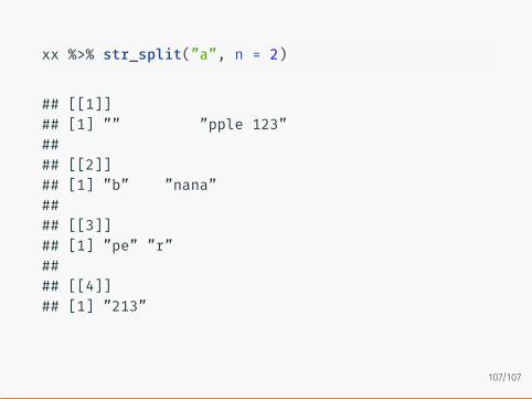
xx %>% str_split(”a”, n = 2)
## [[1]]## [1] ”” ”pple 123”#### [[2]]## [1] ”b” ”nana”#### [[3]]## [1] ”pe” ”r”#### [[4]]## [1] ”213”
107/107