socher & manning's deep learning for nlp...
TRANSCRIPT

Deep Learning for NLP (without Magic)
Richard Socher and Christopher Manning
Stanford University
NAACL 2013, Atlanta h0p://nlp.stanford.edu/courses/NAACL2013/
*with a big thank you to Yoshua Bengio, with whom we parGcipated in the previous ACL 2012 version of this tutorial

Deep Learning
Most current machine learning works well because of human-‐designed representaGons and input features
Machine learning becomes just opGmizing weights to best make a final predicGon
RepresentaGon learning a0empts to automaGcally learn good features or representaGons
Deep learning algorithms a0empt to learn mulGple levels of representaGon of increasing complexity/abstracGon
NER WordNet
SRL Parser
2

A Deep Architecture Mainly, work has explored deep belief networks (DBNs), Markov Random Fields with mulGple layers, and various types of mulGple-‐layer neural networks
Output layer
Here predicGng a supervised target
Hidden layers
These learn more abstract representaGons as you head up
Input layer
Raw sensory inputs (roughly) 3

Five Reasons to Explore Deep Learning
Part 1.1: The Basics
4

#1 Learning representations
5
Handcra^ing features is Gme-‐consuming
The features are o^en both over-‐specified and incomplete
The work has to be done again for each task/domain/…
We must move beyond handcra^ed features and simple ML
Humans develop representaGons for learning and reasoning
Our computers should do the same
Deep learning provides a way of doing this

#2 The need for distributed representations
Current NLP systems are incredibly fragile because of their atomic symbol representaGons
Crazy senten@al complement, such as for “likes [(being) crazy]” 6
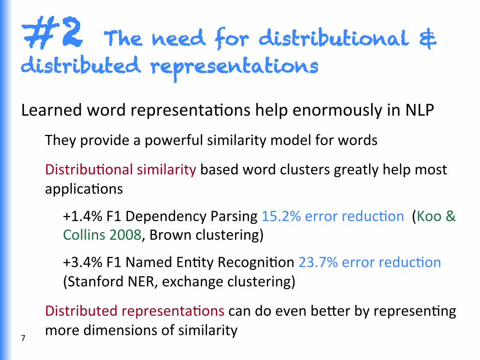
#2 The need for distributional & distributed representations
Learned word representaGons help enormously in NLP
They provide a powerful similarity model for words
DistribuGonal similarity based word clusters greatly help most applicaGons
+1.4% F1 Dependency Parsing 15.2% error reducGon (Koo & Collins 2008, Brown clustering)
+3.4% F1 Named EnGty RecogniGon 23.7% error reducGon (Stanford NER, exchange clustering)
Distributed representaGons can do even be0er by represenGng more dimensions of similarity
7

Learning features that are not mutually exclusive can be exponenGally more efficient than nearest-‐neighbor-‐like or clustering-‐like models
#2 The need for distributed representations
MulG-‐ Clustering Clustering
8
C1 C2 C3
input

Distributed representations deal with the curse of dimensionality
Generalizing locally (e.g., nearest neighbors) requires representaGve examples for all relevant variaGons!
Classic soluGons:
• Manual feature design
• Assuming a smooth target funcGon (e.g., linear models)
• Kernel methods (linear in terms of kernel based on data points)
Neural networks parameterize and learn a “similarity” kernel
9

#3 Unsupervised feature and weight learning
Today, most pracGcal, good NLP& ML methods require labeled training data (i.e., supervised learning)
But almost all data is unlabeled
Most informaGon must be acquired unsupervised
Fortunately, a good model of observed data can really help you learn classificaGon decisions
10

We need good intermediate representaGons that can be shared across tasks
MulGple levels of latent variables allow combinatorial sharing of staGsGcal strength
Insufficient model depth can be exponenGally inefficient
#4 Learning multiple levels of representation
Biologically inspired learning The cortex seems to have a generic learning algorithm
The brain has a deep architecture
Task 1 Output
LinguisGc Input
Task 2 Output Task 3 Output
11

#4 Learning multiple levels of representation
Successive model layers learn deeper intermediate representaGons
Layer 1
Layer 2
Layer 3 High-‐level
linguisGc representaGons
[Lee et al. ICML 2009; Lee et al. NIPS 2009]
12

Handling the recursivity of human language
Human sentences are composed from words and phrases
We need composiGonality in our ML models
Recursion: the same operator (same parameters) is applied repeatedly on different components
A small crowd quietly enters the historic church
historicthe
quietly enters
SVP
Det. Adj.
NPVP
A small crowd
NP
NP
church
N.
Semantic Representations
xt−1 xt xt+1
zt−1 zt zt+1
13

#5 Why now?
Despite prior invesGgaGon and understanding of many of the algorithmic techniques …
Before 2006 training deep architectures was unsuccessful L
What has changed? • New methods for unsupervised pre-‐training have been
developed (Restricted Boltzmann Machines = RBMs, autoencoders, contrasGve esGmaGon, etc.)
• More efficient parameter esGmaGon methods
• Be0er understanding of model regularizaGon
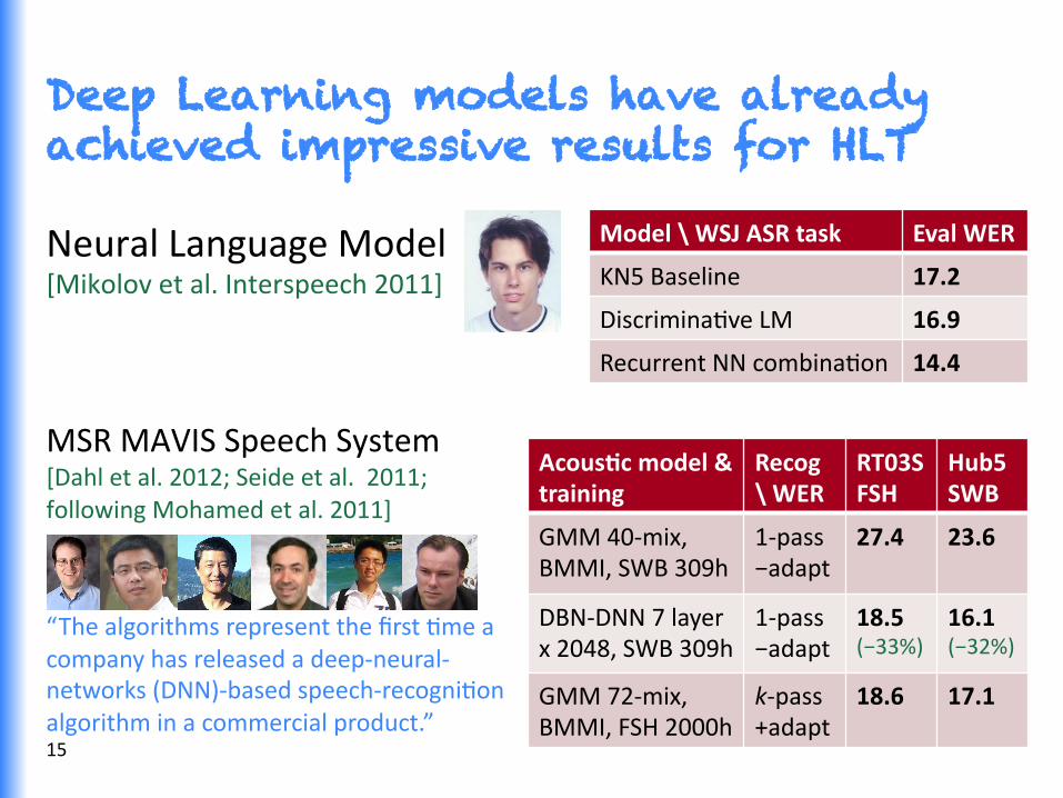
Deep Learning models have already achieved impressive results for HLT
Neural Language Model [Mikolov et al. Interspeech 2011]
MSR MAVIS Speech System [Dahl et al. 2012; Seide et al. 2011; following Mohamed et al. 2011]
“The algorithms represent the first Gme a company has released a deep-‐neural-‐networks (DNN)-‐based speech-‐recogniGon algorithm in a commercial product.”
Model \ WSJ ASR task Eval WER
KN5 Baseline 17.2
DiscriminaGve LM 16.9
Recurrent NN combinaGon 14.4
Acous@c model & training
Recog \ WER
RT03S FSH
Hub5 SWB
GMM 40-‐mix, BMMI, SWB 309h
1-‐pass −adapt
27.4 23.6
DBN-‐DNN 7 layer x 2048, SWB 309h
1-‐pass −adapt
18.5 (−33%)
16.1 (−32%)
GMM 72-‐mix, BMMI, FSH 2000h
k-‐pass +adapt
18.6 17.1
15

Deep Learn Models Have Interesting Performance Characteristics
Deep learning models can now be very fast in some circumstances • SENNA [Collobert et al. 2011] can do POS or NER faster than other SOTA taggers (16x to 122x), using 25x less memory
• WSJ POS 97.29% acc; CoNLL NER 89.59% F1; CoNLL Chunking 94.32% F1
Changes in compuGng technology favor deep learning
• In NLP, speed has tradiGonally come from exploiGng sparsity
• But with modern machines, branches and widely spaced memory accesses are costly
• Uniform parallel operaGons on dense vectors are faster
These trends are even stronger with mulG-‐core CPUs and GPUs
16

17

Outline of the Tutorial
1. The Basics 1. MoGvaGons
2. From logisGc regression to neural networks 3. Word representaGons
4. Unsupervised word vector learning 5. BackpropagaGon Training 6. Learning word-‐level classifiers: POS and NER 7. Sharing staGsGcal strength
2. Recursive Neural Networks 3. ApplicaGons, Discussion, and Resources 18
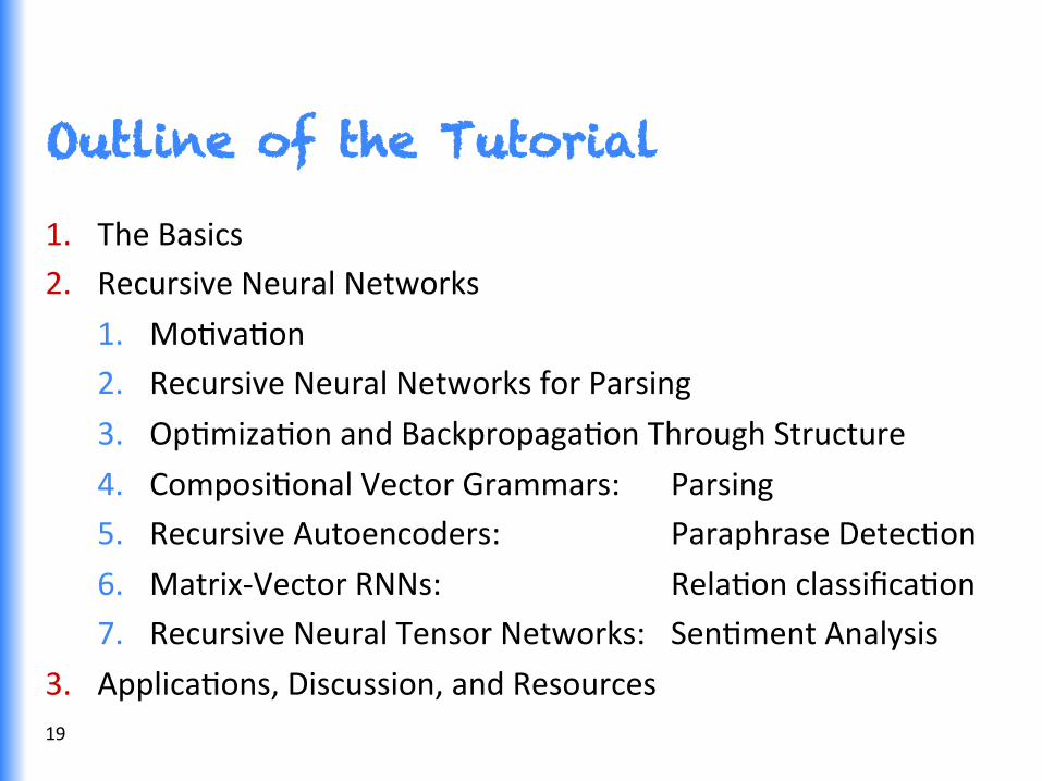
Outline of the Tutorial
1. The Basics 2. Recursive Neural Networks
1. MoGvaGon 2. Recursive Neural Networks for Parsing 3. OpGmizaGon and BackpropagaGon Through Structure
4. ComposiGonal Vector Grammars: Parsing 5. Recursive Autoencoders: Paraphrase DetecGon
6. Matrix-‐Vector RNNs: RelaGon classificaGon 7. Recursive Neural Tensor Networks: SenGment Analysis
3. ApplicaGons, Discussion, and Resources 19

Outline of the Tutorial
1. The Basics 2. Recursive Neural Networks 3. ApplicaGons, Discussion, and Resources
1. Assorted Speech and NLP ApplicaGons 2. Deep Learning: General Strategy and Tricks 3. Resources (readings, code, …) 4. Discussion
20

From logistic regression to neural nets
Part 1.2: The Basics
21
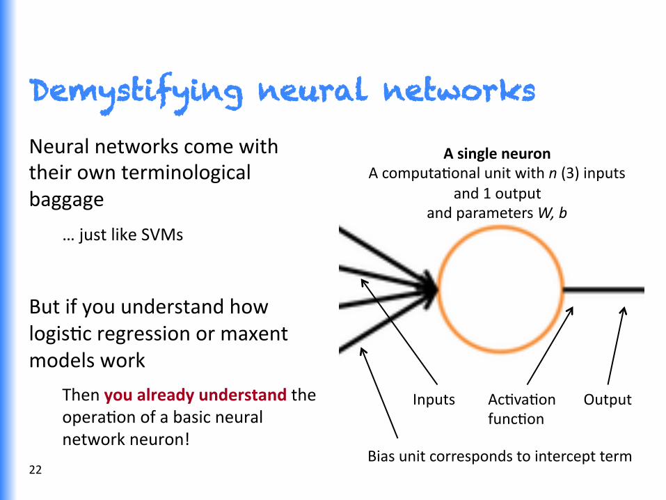
Demystifying neural networks
Neural networks come with their own terminological baggage
… just like SVMs
But if you understand how logisGc regression or maxent models work
Then you already understand the operaGon of a basic neural network neuron!
A single neuron A computaGonal unit with n (3) inputs
and 1 output and parameters W, b
AcGvaGon funcGon
Inputs
Bias unit corresponds to intercept term
Output
22

From Maxent Classifiers to Neural Networks
In NLP, a maxent classifier is normally wri0en as:
Supervised learning gives us a distribuGon for datum d over classes in C
Vector form:
Such a classifier is used as-‐is in a neural network (“a so^max layer”)
• O^en as the top layer: J = so^max(λ·∙x) But for now we’ll derive a two-‐class logisGc model for one neuron
P(c | d,λ) =exp λi fi (c,d)i∑exp λi fi ( "c ,d)i∑"c ∈C∑
P(c | d,λ) = eλT f (c,d )
eλT f ( !c ,d )
!c∑
23
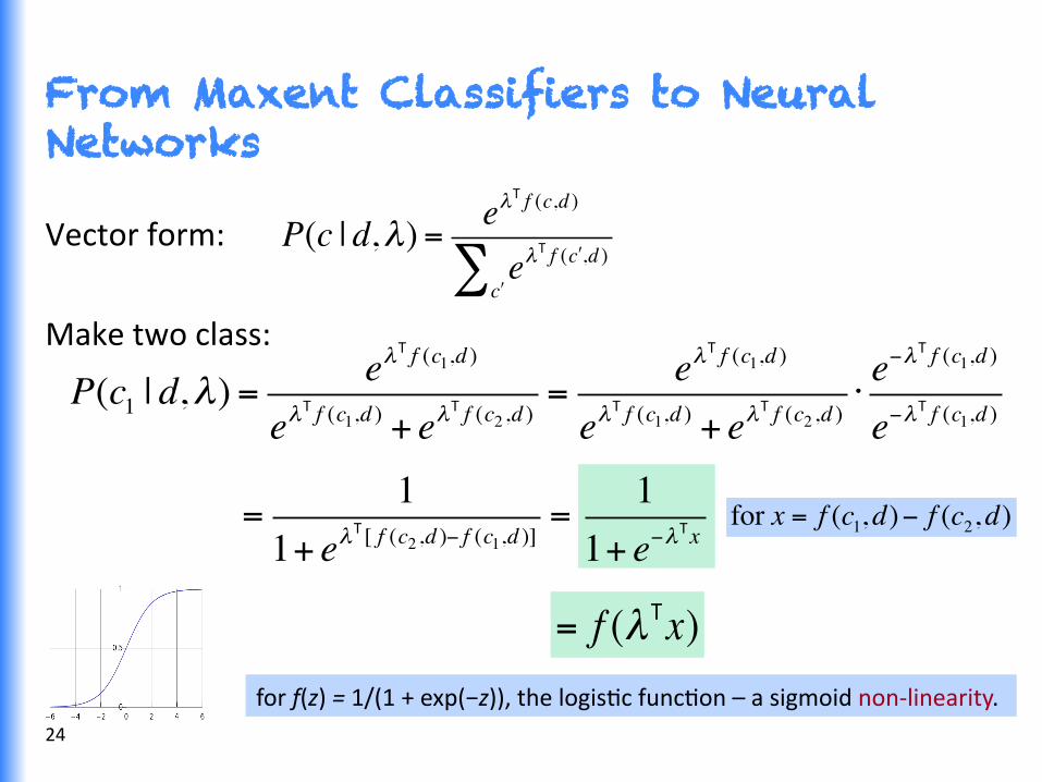
From Maxent Classifiers to Neural Networks
Vector form:
Make two class: P(c1 | d,λ) =
eλT f (c1,d )
eλT f (c1,d ) + eλ
T f (c2 ,d )=
eλT f (c1,d )
eλT f (c1,d ) + eλ
T f (c2 ,d )⋅e−λ
T f (c1,d )
e−λT f (c1,d )
=1
1+ eλT [ f (c2 ,d )− f (c1,d )]
= for x = f (c1,d)− f (c2,d)1
1+ e−λTx
24
= f (λ Tx)
P(c | d,λ) = eλT f (c,d )
eλT f ( !c ,d )
!c∑
for f(z) = 1/(1 + exp(−z)), the logisGc funcGon – a sigmoid non-‐linearity.

This is exactly what a neuron computes
hw,b(x) = f (wTx + b)
f (z) = 11+ e−z
w, b are the parameters of this neuron i.e., this logisGc regression model 25
b: We can have an “always on” feature, which gives a class prior, or separate it out, as a bias term

A neural network = running several logistic regressions at the same time
If we feed a vector of inputs through a bunch of logisGc regression funcGons, then we get a vector of outputs …
But we don’t have to decide ahead of <me what variables these logis<c regressions are trying to predict!
26
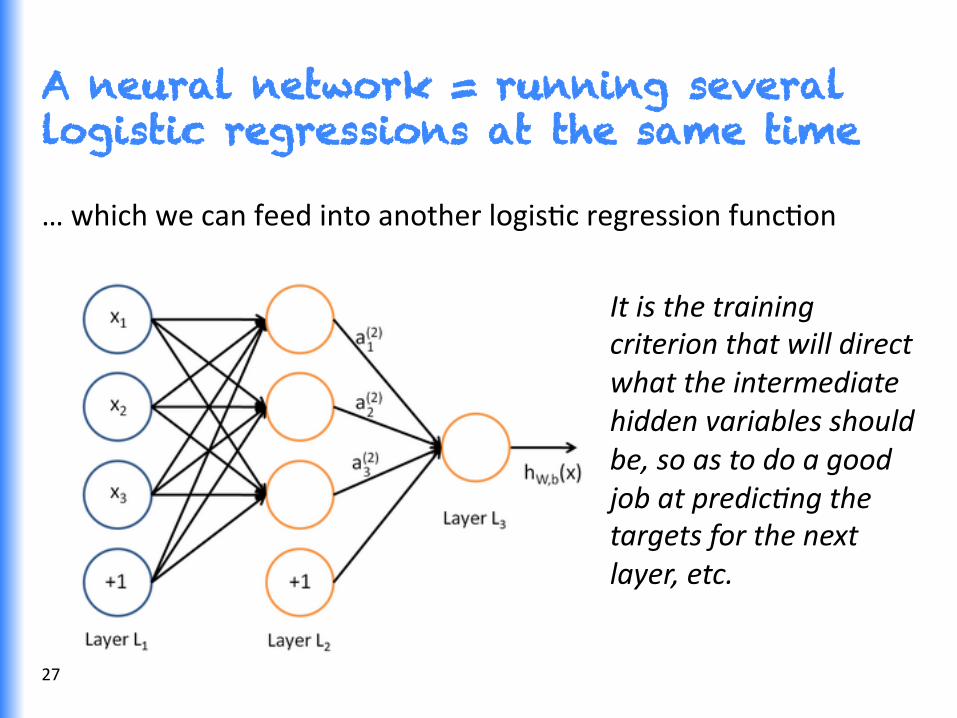
A neural network = running several logistic regressions at the same time
… which we can feed into another logisGc regression funcGon
It is the training criterion that will direct what the intermediate hidden variables should be, so as to do a good job at predic<ng the targets for the next layer, etc.
27

A neural network = running several logistic regressions at the same time
Before we know it, we have a mulGlayer neural network….
28

Matrix notation for a layer
We have
In matrix notaGon
where f is applied element-‐wise:
a1
a2
a3
a1 = f (W11x1 +W12x2 +W13x3 + b1)a2 = f (W21x1 +W22x2 +W23x3 + b2 )etc.
z =Wx + ba = f (z)
f ([z1, z2, z3]) = [ f (z1), f (z2 ), f (z3)]29
W12
b3

How do we train the weights W?
• For a single supervised layer, we train just like a maxent model – we calculate and use error derivaGves (gradients) to improve
• Online learning: StochasGc gradient descent (SGD) • Or improved versions like AdaGrad (Duchi, Hazan, & Singer 2010)
• Batch learning: Conjugate gradient or L-‐BFGS
• A mulGlayer net could be more complex because the internal (“hidden”) logisGc units make the funcGon non-‐convex … just as for hidden CRFs [Qua0oni et al. 2005, Gunawardana et al. 2005] • But we can use the same ideas and techniques • Just without guarantees …
• We “backpropagate” error derivaGves through the model 30

Non-linearities: Why they’re needed
• For logisGc regression: map to probabiliGes • Here: funcGon approximaGon,
e.g., regression or classificaGon • Without non-‐lineariGes, deep neural networks can’t do anything more than a linear transform
• Extra layers could just be compiled down into a single linear transform
• ProbabilisGc interpretaGon unnecessary except in the Boltzmann machine/graphical models
• People o^en use other non-‐lineariGes, such as tanh, as we’ll discuss in part 3
31

Summary Knowing the meaning of words!
You now understand the basics and the relaGon to other models • Neuron = logisGc regression or similar funcGon
• Input layer = input training/test vector • Bias unit = intercept term/always on feature
• AcGvaGon = response • AcGvaGon funcGon is a logisGc (or similar “sigmoid” nonlinearity) • BackpropagaGon = running stochasGc gradient descent backward
layer-‐by-‐layer in a mulGlayer network • Weight decay = regularizaGon / Bayesian prior
32

Effective deep learning became possible through unsupervised pre-training
[Erhan et al., JMLR 2010]
Purely supervised neural net With unsupervised pre-‐training
(with RBMs and Denoising Auto-‐Encoders)
0–9 handwri0en digit recogniGon error rate (MNIST data) 33

Word Representations Part 1.3: The Basics
34

The standard word representation
The vast majority of rule-‐based and staGsGcal NLP work regards words as atomic symbols: hotel, conference, walk
In vector space terms, this is a vector with one 1 and a lot of zeroes
[0 0 0 0 0 0 0 0 0 0 1 0 0 0 0] Dimensionality: 20K (speech) – 50K (PTB) – 500K (big vocab) – 13M (Google 1T)
We call this a “one-‐hot” representaGon. Its problem:
motel [0 0 0 0 0 0 0 0 0 0 1 0 0 0 0] AND hotel [0 0 0 0 0 0 0 1 0 0 0 0 0 0 0] = 0
35

Distributional similarity based representations
You can get a lot of value by represenGng a word by means of its neighbors
“You shall know a word by the company it keeps” (J. R. Firth 1957: 11)
One of the most successful ideas of modern staGsGcal NLP
government debt problems turning into banking crises as has happened in
saying that Europe needs unified banking regulation to replace the hodgepodge
ë These words will represent banking ì
36
You can vary whether you use local or large context to get a more syntacGc or semanGc clustering

Class-based (hard) and soft clustering word representations
Class based models learn word classes of similar words based on distribuGonal informaGon ( ~ class HMM)
• Brown clustering (Brown et al. 1992) • Exchange clustering (MarGn et al. 1998, Clark 2003) • DesparsificaGon and great example of unsupervised pre-‐training
So^ clustering models learn for each cluster/topic a distribuGon over words of how likely that word is in each cluster
• Latent SemanGc Analysis (LSA/LSI), Random projecGons • Latent Dirichlet Analysis (LDA), HMM clustering
37

Neural word embeddings as a distributed representation
Similar idea
Combine vector space semanGcs with the predicGon of probabilisGc models (Bengio et al. 2003, Collobert & Weston 2008, Turian et al. 2010)
In all of these approaches, including deep learning models, a word is represented as a dense vector
linguis<cs =
38
0.286 0.792 −0.177 −0.107 0.109 −0.542 0.349 0.271

Neural word embeddings - visualization
39

Stunning new result at this conference! Mikolov, Yih & Zweig (NAACL 2013)
These representaGons are way be0er at encoding dimensions of similarity than we realized!
• Analogies tesGng dimensions of similarity can be solved quite well just by doing vector subtracGon in the embedding space SyntacGcally
• xapple − xapples ≈ xcar − xcars ≈ xfamily − xfamilies
• Similarly for verb and adjecGve morphological forms SemanGcally (Semeval 2012 task 2)
• xshirt − xclothing ≈ xchair − xfurniture
40

Stunning new result at this conference! Mikolov, Yih & Zweig (NAACL 2013)
Method Syntax % correct
LSA 320 dim 16.5 [best]
RNN 80 dim 16.2
RNN 320 dim 28.5
RNN 1600 dim 39.6
Method Seman@cs Spearm ρ
UTD-‐NB (Rink & H. 2012) 0.230 [Semeval win]
LSA 640 0.149
RNN 80 0.211
RNN 1600 0.275 [new SOTA]
41

Advantages of the neural word embedding approach
42
Compared to a method like LSA, neural word embeddings can become more meaningful through adding supervision from one or mulGple tasks
“DiscriminaGve fine-‐tuning”
For instance, senGment is usually not captured in unsupervised word embeddings but can be in neural word vectors
We can build representaGons for large linguisGc units
See part 2

Unsupervised word vector learning
Part 1.4: The Basics
43

A neural network for learning word vectors (Collobert et al. JMLR 2011)
Idea: A word and its context is a posiGve training sample; a random word in that same context gives a negaGve training sample:
cat chills on a mat cat chills Jeju a mat
Similar: Implicit negaGve evidence in ContrasGve EsGmaGon, (Smith and Eisner 2005)
44

A neural network for learning word vectors
45
How do we formalize this idea? Ask that
score(cat chills on a mat) > score(cat chills Jeju a mat)
How do we compute the score?
• With a neural network • Each word is associated with an
n-‐dimensional vector

Word embedding matrix
• IniGalize all word vectors randomly to form a word embedding matrix |V|
L = … n
the cat mat …
• These are the word features we want to learn • Also called a look-‐up table
• Conceptually you get a word’s vector by le^ mulGplying a one-‐hot vector e by L: x = Le
[ ]
46

• score(cat chills on a mat) • To describe a phrase, retrieve (via index) the corresponding
vectors from L
cat chills on a mat
• Then concatenate them to 5n vector: • x =[ ]
• How do we then compute score(x)?
Word vectors as input to a neural network
47

A Single Layer Neural Network
• A single layer was a combinaGon of a linear layer and a nonlinearity:
• The neural acGvaGons a can then be used to compute some funcGon
• For instance, the score we care about:
48

Summary: Feed-forward Computation
49
CompuGng a window’s score with a 3-‐layer Neural Net: s = score(cat chills on a mat)
cat chills on a mat

Summary: Feed-forward Computation
• s = score(cat chills on a mat) • sc = score(cat chills Jeju a mat)
• Idea for training objecGve: make score of true window larger and corrupt window’s score lower (unGl they’re good enough): minimize
• This is conGnuous, can perform SGD 50
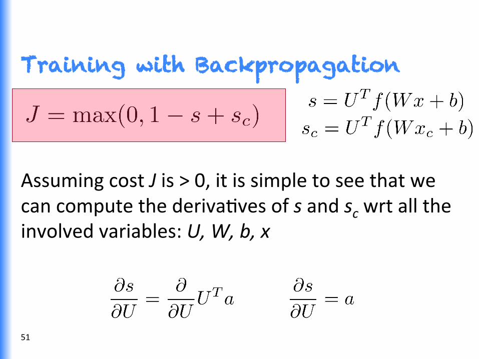
Training with Backpropagation
Assuming cost J is > 0, it is simple to see that we can compute the derivaGves of s and sc wrt all the involved variables: U, W, b, x
51

Training with Backpropagation
• Let’s consider the derivaGve of a single weight Wij
• This only appears inside ai
• For example: W23 is only used to compute a2
x1 x2 x3 +1
a1 a2
s U2
W23
52

Training with Backpropagation
DerivaGve of weight Wij:
53 x1 x2 x3 +1
a1 a2
s U2
W23
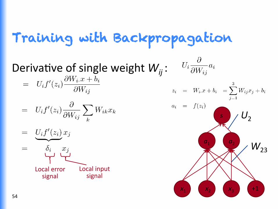
Training with Backpropagation
DerivaGve of single weight Wij :
Local error signal
Local input signal
54 x1 x2 x3 +1
a1 a2
s U2
W23

• We want all combinaGons of i = 1, 2 and j = 1, 2, 3
• SoluGon: Outer product: where is the “responsibility” coming from each acGvaGon a
Training with Backpropagation
• From single weight Wij to full W:
55 x1 x2 x3 +1
a1 a2
s U2
W23

Training with Backpropagation
• For biases b, we get:
56 x1 x2 x3 +1
a1 a2
s U2
W23
Training with Backpropagation
57
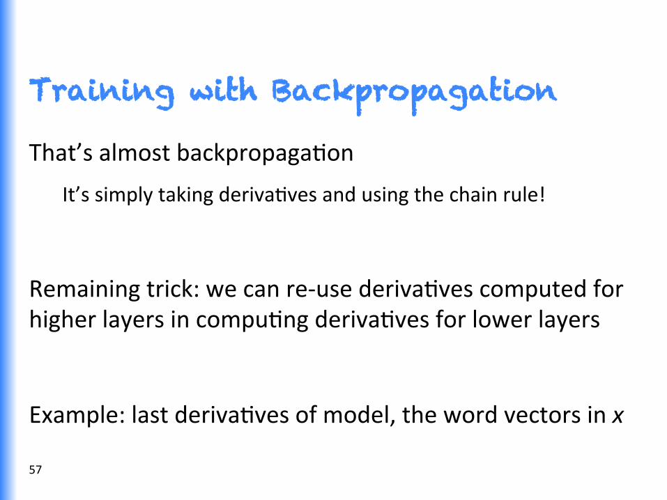
That’s almost backpropagaGon
It’s simply taking derivaGves and using the chain rule!
Remaining trick: we can re-‐use derivaGves computed for higher layers in compuGng derivaGves for lower layers
Example: last derivaGves of model, the word vectors in x

Training with Backpropagation
• Take derivaGve of score with respect to single word vector (for simplicity a 1d vector, but same if it was longer)
• Now, we cannot just take into consideraGon one ai because each xj is connected to all the neurons above and hence xj influences the overall score through all of these, hence:
Re-‐used part of previous derivaGve 58

Training with Backpropagation: softmax
59
What is the major benefit of deep learned word vectors?
Ability to also propagate labeled informaGon into them, via so^max/maxent and hidden layer:
S
c1 c2 c3
x1 x2 x3 +1
a1 a2 P(c | d,λ) = eλ
T f (c,d )
eλT f ( !c ,d )
!c∑

Backpropagation Training Part 1.5: The Basics
60

Back-Prop
• Compute gradient of example-‐wise loss wrt parameters
• Simply applying the derivaGve chain rule wisely
• If compuGng the loss(example, parameters) is O(n) computaGon, then so is compuGng the gradient
61

Simple Chain Rule
62

Multiple Paths Chain Rule
63

Multiple Paths Chain Rule - General
…
64

Chain Rule in Flow Graph
…
…
…
Flow graph: any directed acyclic graph node = computaGon result arc = computaGon dependency
= successors of
65

Back-Prop in Multi-Layer Net
…
…
66
h = sigmoid(Vx)

Back-Prop in General Flow Graph
…
…
…
= successors of
1. Fprop: visit nodes in topo-‐sort order -‐ Compute value of node given predecessors
2. Bprop: -‐ iniGalize output gradient = 1 -‐ visit nodes in reverse order:
Compute gradient wrt each node using gradient wrt successors
Single scalar output
67
Automatic Differentiation
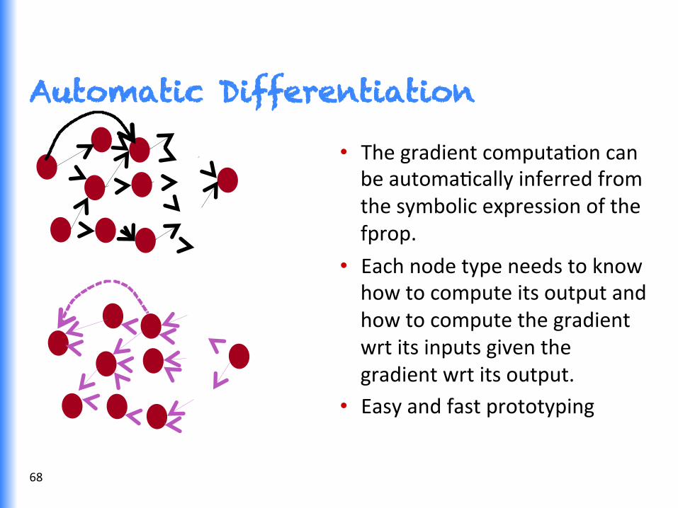
• The gradient computaGon can be automaGcally inferred from the symbolic expression of the fprop.
• Each node type needs to know how to compute its output and how to compute the gradient wrt its inputs given the gradient wrt its output.
• Easy and fast prototyping
68

Learning word-level classifiers: POS and NER
Part 1.6: The Basics
69

The Model (Collobert & Weston 2008; Collobert et al. 2011)
• Similar to word vector learning but replaces the single scalar score with a SoLmax/Maxent classifier
• Training is again done via backpropagaGon which gives an error similar to the score in the unsupervised word vector learning model
70
S
c1 c2 c3
x1 x2 x3 +1
a1 a2

The Model - Training
• We already know the so^max classifier and how to opGmize it • The interesGng twist in deep learning is that the input features
are also learned, similar to learning word vectors with a score:
S
c1 c2 c3
x1 x2 x3 +1
a1 a2
s U2
W23
x1 x2 x3 +1
a1 a2
71

POS WSJ (acc.)
NER CoNLL (F1)
State-‐of-‐the-‐art* 97.24 89.31 Supervised NN 96.37 81.47 Unsupervised pre-‐training followed by supervised NN**
97.20 88.87
+ hand-‐cra^ed features*** 97.29 89.59
* RepresentaGve systems: POS: (Toutanova et al. 2003), NER: (Ando & Zhang 2005)
** 130,000-‐word embedding trained on Wikipedia and Reuters with 11 word window, 100 unit hidden layer – for 7 weeks! – then supervised task training
***Features are character suffixes for POS and a gaze0eer for NER
The secret sauce is the unsupervised pre-training on a large text collection
72

POS WSJ (acc.)
NER CoNLL (F1)
Supervised NN 96.37 81.47
NN with Brown clusters 96.92 87.15
Fixed embeddings* 97.10 88.87
C&W 2011** 97.29 89.59
* Same architecture as C&W 2011, but word embeddings are kept constant during the supervised training phase
** C&W is unsupervised pre-‐train + supervised NN + features model of last slide
Supervised refinement of the unsupervised word representation helps
73

Sharing statistical strength Part 1.7
74

Multi-Task Learning
• Generalizing be0er to new tasks is crucial to approach AI
• Deep architectures learn good intermediate representaGons that can be shared across tasks
• Good representaGons make sense for many tasks
raw input x
task 1 output y1
task 3 output y3
task 2 output y2
shared intermediate representation h
75
Combining Multiple Sources of Evidence with Shared Embeddings
• RelaGonal learning • MulGple sources of informaGon / relaGons • Some symbols (e.g. words, wikipedia entries) shared
• Shared embeddings help propagate informaGon among data sources: e.g., WordNet, XWN, Wikipedia, FreeBase, …
76

Sharing Statistical Strength
• Besides very fast predicGon, the main advantage of deep learning is staGsGcal
• PotenGal to learn from less labeled examples because of sharing of staGsGcal strength:
• Unsupervised pre-‐training & mulG-‐task learning • Semi-‐supervised learning à
77

Semi-Supervised Learning
• Hypothesis: P(c|x) can be more accurately computed using shared structure with P(x)
purely supervised
78

Semi-Supervised Learning
• Hypothesis: P(c|x) can be more accurately computed using shared structure with P(x)
semi-‐ supervised
79

Deep autoencoders
AlternaGve to contrasGve unsupervised word learning • Another is RBMs (Hinton et al. 2006), which we don’t cover today
Works well for fixed input representaGons
1. DefiniGon, intuiGon and variants of autoencoders 2. Stacking for deep autoencoders 3. Why do autoencoders improve deep neural nets so much?
80

Auto-Encoders
• MulGlayer neural net with target output = input • ReconstrucGon=decoder(encoder(input))
• Probable inputs have small reconstrucGon error
…
code= latent features
… encoder
decoder
input
reconstrucGon
81
PCA = Linear Manifold = Linear Auto-Encoder
reconstrucGon error vector
Linear manifold
reconstrucGon(x)
x
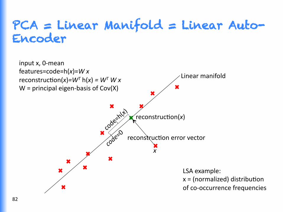
input x, 0-‐mean features=code=h(x)=W x reconstrucGon(x)=WT h(x) = WT W x W = principal eigen-‐basis of Cov(X)
LSA example: x = (normalized) distribuGon of co-‐occurrence frequencies
82

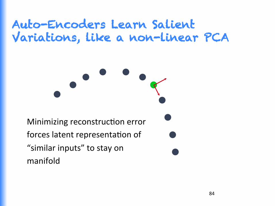
The Manifold Learning Hypothesis
• Examples concentrate near a lower dimensional “manifold” (region of high density where small changes are only allowed in certain direcGons)
83
84
Auto-Encoders Learn Salient Variations, like a non-linear PCA
Minimizing reconstrucGon error forces latent representaGon of
“similar inputs” to stay on manifold

Auto-Encoder Variants • Discrete inputs: cross-‐entropy or log-‐likelihood reconstrucGon
criterion (similar to used for discrete targets for MLPs)
• PrevenGng them to learn the idenGty everywhere: • Undercomplete (eg PCA): bo0leneck code smaller than input
• Sparsity: penalize hidden unit acGvaGons so at or near 0 [Goodfellow et al 2009]
• Denoising: predict true input from corrupted input [Vincent et al 2008]
• ContracGve: force encoder to have small derivaGves
[Rifai et al 2011] 85

Sparse autoencoder illustration for images
Natural Images
Learned bases: “Edges”
50 100 150 200 250 300 350 400 450 500
50
100
150
200
250
300
350
400
450
500
50 100 150 200 250 300 350 400 450 500
50
100
150
200
250
300
350
400
450
500
50 100 150 200 250 300 350 400 450 500
50
100
150
200
250
300
350
400
450
500
≈ 0.8 * + 0.3 * + 0.5 *
x ≈ 0.8 * φ36 + 0.3 * φ42
+ 0.5 * φ63
[a1, …, a64] = [0, 0, …, 0, 0.8, 0, …, 0, 0.3, 0, …, 0, 0.5, 0] (feature representaGon)
Test example
86
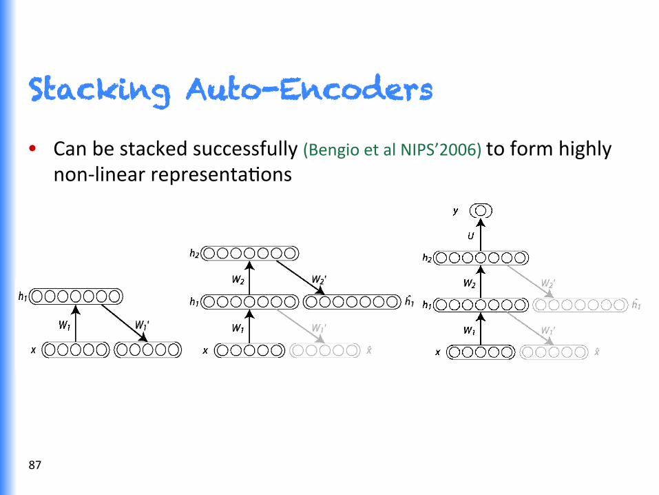
Stacking Auto-Encoders
• Can be stacked successfully (Bengio et al NIPS’2006) to form highly non-‐linear representaGons
87

Layer-wise Unsupervised Learning
… input
88

Layer-wise Unsupervised Pre-training
…
…
input
features
89

Layer-wise Unsupervised Pre-training
…
…
…
input
features
reconstruction of input =
? … input
90

Layer-wise Unsupervised Pre-training
…
…
input
features
91

Layer-wise Unsupervised Pre-training
…
…
input
features
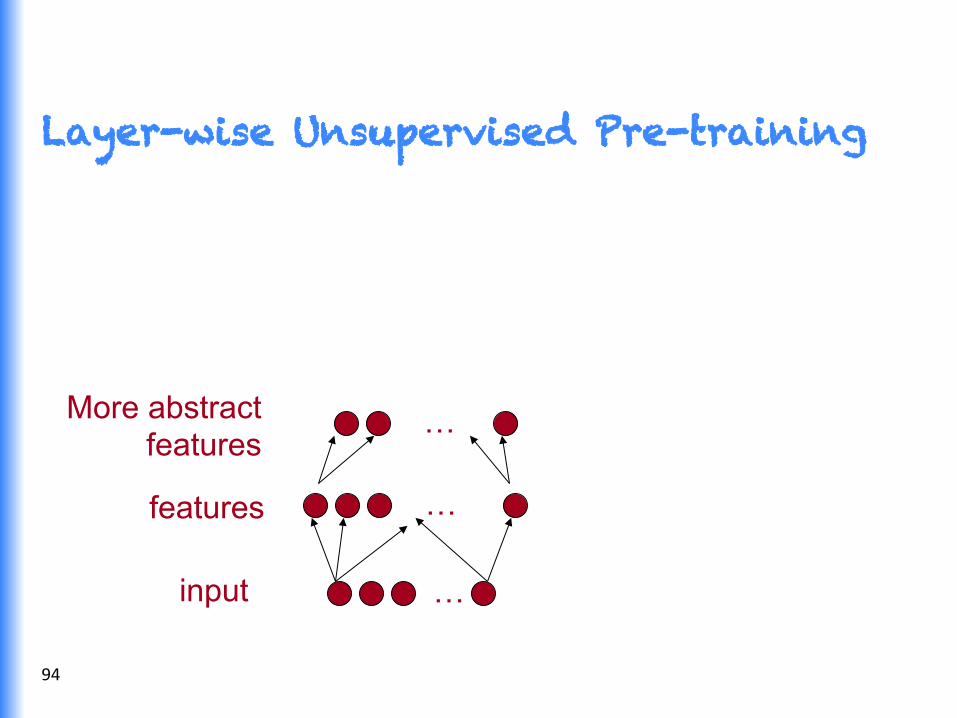
… More abstract features
92

…
…
input
features
… More abstract features
reconstruction of features =
? … … … …
Layer-Wise Unsupervised Pre-training Layer-wise Unsupervised Learning
93
…
…
input
features
… More abstract features
Layer-wise Unsupervised Pre-training
94

…
…
input
features
… More abstract features
… Even more abstract
features
Layer-wise Unsupervised Learning
95

…
…
input
features
… More abstract features
… Even more abstract
features
Output f(X) six
Target Y
two! = ?
Supervised Fine-Tuning
96

Why is unsupervised pre-training working so well?
• RegularizaGon hypothesis: • RepresentaGons good for P(x) are good for P(y|x)
• OpGmizaGon hypothesis: • Unsupervised iniGalizaGons start near be0er local minimum of supervised training error
• Minima otherwise not achievable by random iniGalizaGon
Erhan, Courville, Manzagol, Vincent, Bengio (JMLR, 2010) 97

Recursive Deep Learning Part 2
98

Building on Word Vector Space Models
99
x2
x1 0 1 2 3 4 5 6 7 8 9 10
5
4
3
2
1 Monday
9 2
Tuesday 9.5 1.5
By mapping them into the same vector space!
1 5
1.1 4
the country of my birth the place where I was born
But how can we represent the meaning of longer phrases?
France 2 2.5
Germany 1 3

How should we map phrases into a vector space?
the country of my birth
0.4 0.3
2.3 3.6
4 4.5
7 7
2.1 3.3
2.5 3.8
5.5 6.1
1 3.5
1 5
Use principle of composiGonality
The meaning (vector) of a sentence is determined by (1) the meanings of its words and (2) the rules that combine them.
Models in this secGon can jointly learn parse trees and composiGonal vector representaGons
x2
x1 0 1 2 3 4 5 6 7 8 9 10
5
4
3
2
1
the country of my birth
the place where I was born
Monday
Tuesday
France
Germany
100

Semantic Vector Spaces
• DistribuGonal Techniques • Brown Clusters
• Useful as features inside models, e.g. CRFs for NER, etc.
• Cannot capture longer phrases
Single Word Vectors Documents Vectors
• Bag of words models • LSA, LDA
• Great for IR, document exploraGon, etc.
• Ignore word order, no detailed understanding
Vectors represenGng Phrases and Sentences that do not ignore word order and capture semanGcs for NLP tasks

Recursive Deep Learning
1. MoGvaGon 2. Recursive Neural Networks for Parsing 3. OpGmizaGon and BackpropagaGon Through Structure 4. ComposiGonal Vector Grammars: Parsing
5. Recursive Autoencoders: Paraphrase DetecGon
6. Matrix-‐Vector RNNs: RelaGon classificaGon 7. Recursive Neural Tensor Networks: SenGment Analysis
102

Sentence Parsing: What we want
9 1
5 3
8 5
9 1
4 3
NP NP
PP
S
7 1
VP
The cat sat on the mat. 103

Learn Structure and Representation
NP NP
PP
S
VP
5 2 3
3
8 3
5 4
7 3
The cat sat on the mat.
9 1
5 3
8 5
9 1
4 3
7 1
104

Recursive Neural Networks for Structure Prediction
on the mat.
9 1
4 3
3 3
8 3
8 5
3 3
Neural "Network"
8 3
1.3
Inputs: two candidate children’s representaGons Outputs: 1. The semanGc representaGon if the two nodes are merged. 2. Score of how plausible the new node would be.
8 5
105

Recursive Neural Network Definition
score = UTp
p = tanh(W + b),
Same W parameters at all nodes of the tree
8 5
3 3
Neural "Network"
8 3
1.3 score = = parent
c1 c2
c1 c2
106

Related Work to Socher et al. (ICML 2011)
• Pollack (1990): Recursive auto-‐associaGve memories
• Previous Recursive Neural Networks work by Goller & Küchler (1996), Costa et al. (2003) assumed fixed tree structure and used one hot vectors.
• Hinton (1990) and Bo0ou (2011): Related ideas about recursive models and recursive operators as smooth versions of logic operaGons
107

Parsing a sentence with an RNN
Neural "Network"
0.1 2 0
Neural "Network"
0.4 1 0
Neural "Network"
2.3 3 3
9 1
5 3
8 5
9 1
4 3
7 1
Neural "Network"
3.1 5 2
Neural "Network"
0.3 0 1
The cat sat on the mat.
108

Parsing a sentence
9 1
5 3
5 2
Neural "Network"
1.1 2 1
The cat sat on the mat.
Neural "Network"
0.1 2 0
Neural "Network"
0.4 1 0
Neural "Network"
2.3 3 3
5 3
8 5
9 1
4 3
7 1
109

Parsing a sentence
5 2
Neural "Network"
1.1 2 1
Neural "Network"
0.1 2 0
3 3
Neural "Network"
3.6 8 3
9 1
5 3
The cat sat on the mat.
5 3
8 5
9 1
4 3
7 1
110

Parsing a sentence
5 2
3 3
8 3
5 4
7 3
9 1
5 3
The cat sat on the mat.
5 3
8 5
9 1
4 3
7 1
111

Max-Margin Framework - Details • The score of a tree is computed by
the sum of the parsing decision scores at each node.
• Similar to max-‐margin parsing (Taskar et al. 2004), a supervised max-‐margin objecGve
• The loss penalizes all incorrect decisions • Structure search for A(x) was maximally greedy
• Instead: Beam Search with Chart
8 5
3 3
RNN"
8 3 1.3
112
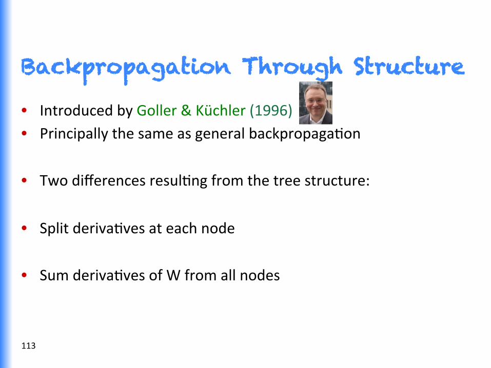
Backpropagation Through Structure
• Introduced by Goller & Küchler (1996) • Principally the same as general backpropagaGon
• Two differences resulGng from the tree structure:
• Split derivaGves at each node
• Sum derivaGves of W from all nodes
113

BTS: Split derivatives at each node • During forward prop, the parent is computed using 2 children
• Hence, the errors need to be computed wrt each of them:
where each child’s error is n-‐dimensional
8 5
3 3
8 3
c1 p = tanh(W + b) c1
c2 c2
8 5
3 3
8 3
c1 c2
114

BTS: Sum derivatives of all nodes • You can actually assume it’s a different W at each node • IntuiGon via example:
• If take separate derivaGves of each occurrence, we get same:
115

BTS: Optimization
• As before, we can plug the gradients into a standard off-‐the-‐shelf L-‐BFGS opGmizer
• Best results with AdaGrad (Duchi et al, 2011):
• For non-‐conGnuous objecGve use subgradient method (Ratliff et al. 2007)
116

Discussion: Simple RNN • Good results with single matrix RNN (more later)
• Single weight matrix RNN could capture some phenomena but not adequate for more complex, higher order composiGon and parsing long sentences
• The composiGon funcGon is the same for all syntacGc categories, punctuaGon, etc
W
c1 c2
pWscore s

Solution: Syntactically-Untied RNN • Idea: CondiGon the composiGon funcGon on the syntacGc categories, “unGe the weights”
• Allows for different composiGon funcGons for pairs of syntacGc categories, e.g. Adv + AdjP, VP + NP
• Combines discrete syntacGc categories with conGnuous semanGc informaGon

Solution: CVG = PCFG + Syntactically-Untied RNN • Problem: Speed. Every candidate score in beam search needs a matrix-‐vector product.
• SoluGon: Compute score using a linear combinaGon of the log-‐likelihood from a simple PCFG + RNN
• Prunes very unlikely candidates for speed • Provides coarse syntacGc categories of the children for each beam candidate
• ComposiGonal Vector Grammars: CVG = PCFG + RNN

Details: Compositional Vector Grammar
• Scores at each node computed by combinaGon of PCFG and SU-‐RNN:
• InterpretaGon: Factoring discrete and conGnuous parsing in one model:
• Socher et al (2013): More details at ACL

Related Work • ResulGng CVG Parser is related to previous work that extends PCFG
parsers • Klein and Manning (2003a) : manual feature engineering
• Petrov et al. (2006) : learning algorithm that splits and merges syntacGc categories
• Lexicalized parsers (Collins, 2003; Charniak, 2000): describe each category with a lexical item
• Hall and Klein (2012) combine several such annotaGon schemes in a factored parser.
• CVGs extend these ideas from discrete representaGons to richer conGnuous ones
• Hermann & Blunsom (2013): Combine Combinatory Categorial Grammars with RNNs and also unGe weights, see upcoming ACL 2013

Experiments • Standard WSJ split, labeled F1 • Based on simple PCFG with fewer states
• Fast pruning of search space, few matrix-‐vector products • 3.8% higher F1, 20% faster than Stanford parser
Parser Test, All Sentences
Stanford PCFG, (Klein and Manning, 2003a) 85.5
Stanford Factored (Klein and Manning, 2003b) 86.6
Factored PCFGs (Hall and Klein, 2012) 89.4
Collins (Collins, 1997) 87.7
SSN (Henderson, 2004) 89.4
Berkeley Parser (Petrov and Klein, 2007) 90.1
CVG (RNN) (Socher et al., ACL 2013) 85.0
CVG (SU-‐RNN) (Socher et al., ACL 2013) 90.4
Charniak -‐ Self Trained (McClosky et al. 2006) 91.0
Charniak -‐ Self Trained-‐ReRanked (McClosky et al. 2006) 92.1
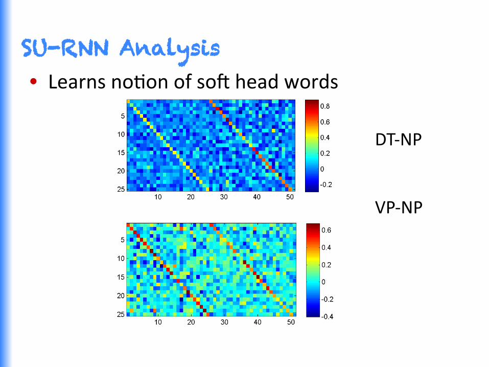
SU-RNN Analysis • Learns noGon of so^ head words
DT-‐NP VP-‐NP

Analysis of resulting vector representations
All the figures are adjusted for seasonal variaGons 1. All the numbers are adjusted for seasonal fluctuaGons 2. All the figures are adjusted to remove usual seasonal pa0erns
Knight-‐Ridder wouldn’t comment on the offer 1. Harsco declined to say what country placed the order 2. Coastal wouldn’t disclose the terms
Sales grew almost 7% to $UNK m. from $UNK m. 1. Sales rose more than 7% to $94.9 m. from $88.3 m. 2. Sales surged 40% to UNK b. yen from UNK b.
"

SU-RNN Analysis
• Can transfer semanGc informaGon from single related example
• Train sentences: • He eats spaghe� with a fork.
• She eats spaghe� with pork.
• Test sentences • He eats spaghe� with a spoon.
• He eats spaghe� with meat.

SU-RNN Analysis

Labeling in Recursive Neural Networks
Neural "Network"
8 3
• We can use each node’s representaGon as features for a soLmax classifier:
• Training similar to model in part 1 with standard cross-‐entropy error + scores
Softmax"Layer"
NP
127

Scene Parsing
• The meaning of a scene image is also a funcGon of smaller regions,
• how they combine as parts to form larger objects,
• and how the objects interact.
Similar principle of composiGonality.
128

Algorithm for Parsing Images Same Recursive Neural Network as for natural language parsing!
(Socher et al. ICML 2011)
Features
Grass Tree
Segments
Semantic Representations
People Building
Parsing Natural Scene ImagesParsing Natural Scene Images
129
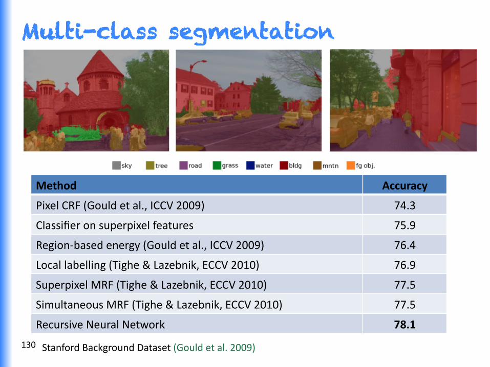
Multi-class segmentation
Method Accuracy
Pixel CRF (Gould et al., ICCV 2009) 74.3
Classifier on superpixel features 75.9
Region-‐based energy (Gould et al., ICCV 2009) 76.4
Local labelling (Tighe & Lazebnik, ECCV 2010) 76.9
Superpixel MRF (Tighe & Lazebnik, ECCV 2010) 77.5
Simultaneous MRF (Tighe & Lazebnik, ECCV 2010) 77.5
Recursive Neural Network 78.1
Stanford Background Dataset (Gould et al. 2009) 130

Recursive Deep Learning
1. MoGvaGon 2. Recursive Neural Networks for Parsing 3. Theory: BackpropagaGon Through Structure 4. ComposiGonal Vector Grammars: Parsing
5. Recursive Autoencoders: Paraphrase DetecGon
6. Matrix-‐Vector RNNs: RelaGon classificaGon 7. Recursive Neural Tensor Networks: SenGment Analysis
131

Semi-supervised Recursive Autoencoder • To capture senGment and solve antonym problem, add a so^max classifier
• Error is a weighted combinaGon of reconstrucGon error and cross-‐entropy • Socher et al. (EMNLP 2011)
Reconstruction error Cross-‐entropy error
W(1)
W(2)
W(label)
132

Paraphrase Detection
• Pollack said the plainGffs failed to show that Merrill and Blodget directly caused their losses
• Basically , the plainGffs did not show that omissions in Merrill’s research caused the claimed losses
• The iniGal report was made to Modesto Police December 28
• It stems from a Modesto police report
133

How to compare the meaning
of two sentences?
134
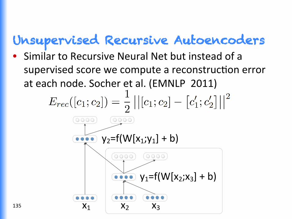
Unsupervised Recursive Autoencoders • Similar to Recursive Neural Net but instead of a supervised score we compute a reconstrucGon error at each node. Socher et al. (EMNLP 2011)
x2 x3x1
y1=f(W[x2;x3] + b)
y2=f(W[x1;y1] + b)
135

Unsupervised unfolding RAE
136
• A0empt to encode enGre tree structure at each node

Recursive Autoencoders for Full Sentence Paraphrase Detection
• Unsupervised Unfolding RAE and a pair-‐wise sentence comparison of nodes in parsed trees
• Socher et al. (NIPS 2011)
137
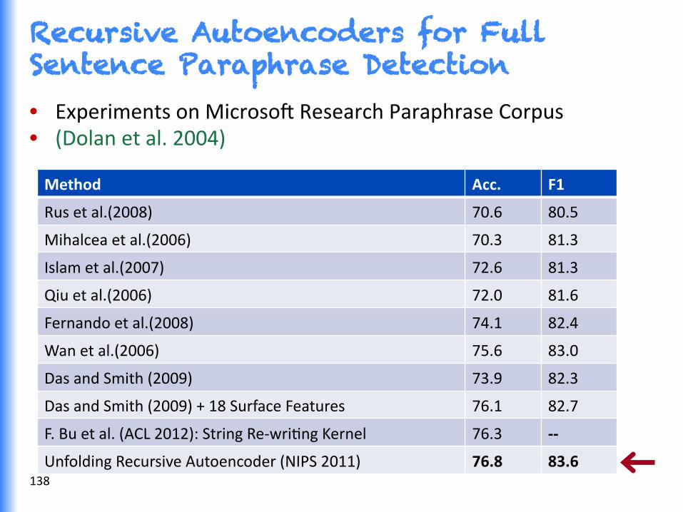
Recursive Autoencoders for Full Sentence Paraphrase Detection • Experiments on Microso^ Research Paraphrase Corpus • (Dolan et al. 2004)
Method Acc. F1
Rus et al.(2008) 70.6 80.5
Mihalcea et al.(2006) 70.3 81.3
Islam et al.(2007) 72.6 81.3
Qiu et al.(2006) 72.0 81.6
Fernando et al.(2008) 74.1 82.4
Wan et al.(2006) 75.6 83.0
Das and Smith (2009) 73.9 82.3
Das and Smith (2009) + 18 Surface Features 76.1 82.7
F. Bu et al. (ACL 2012): String Re-‐wriGng Kernel 76.3 -‐-‐
Unfolding Recursive Autoencoder (NIPS 2011) 76.8 83.6 138

Recursive Autoencoders for Full Sentence Paraphrase Detection
139

Recursive Deep Learning
1. MoGvaGon 2. Recursive Neural Networks for Parsing 3. Theory: BackpropagaGon Through Structure 4. ComposiGonal Vector Grammars: Parsing
5. Recursive Autoencoders: Paraphrase DetecGon
6. Matrix-‐Vector RNNs: RelaGon classificaGon 7. Recursive Neural Tensor Networks: SenGment Analysis
140

Compositionality Through Recursive Matrix-Vector Spaces
• One way to make the composiGon funcGon more powerful was by untying the weights W
• But what if words act mostly as an operator, e.g. “very” in very good
• Proposal: A new composiGon funcGon
p = tanh(W + b)
c1 c2
141

Compositionality Through Recursive Matrix-Vector Recursive Neural Networks
p = tanh(W + b)
c1 c2
p = tanh(W + b)
C2c1 C1c2
142

Predicting Sentiment Distributions • Good example for non-‐linearity in language
143

MV-RNN for Relationship Classification
Rela@onship Sentence with labeled nouns for which to predict rela@onships
Cause-‐Effect(e2,e1)
Avian [influenza]e1 is an infecGous disease caused by type a strains of the influenza [virus]e2.
EnGty-‐Origin(e1,e2)
The [mother]e1 le^ her naGve [land]e2 about the same Gme and they were married in that city.
Message-‐Topic(e2,e1)
Roadside [a0racGons]e1 are frequently adverGsed with [billboards]e2 to a0ract tourists.
144

Sentiment Detection • SenGment detecGon is crucial to business intelligence, stock trading, …
145

Sentiment Detection and Bag-of-Words Models
• Most methods start with a bag of words + linguisGc features/processing/lexica
• But such methods (including �-‐idf) can’t disGnguish: + white blood cells destroying an infecGon -‐ an infecGon destroying white blood cells
146

Sentiment Detection and Bag-of-Words Models • SenGment is that senGment is “easy” • DetecGon accuracy for longer documents ~90%
• Lots of easy cases (… horrible… or … awesome …)
• For dataset of single sentence movie reviews (Pang and Lee, 2005) accuracy never reached above 80% for >7 years
• Harder cases require actual understanding of negaGon and its scope and other semanGc effects

Data: Movie Reviews
Stealing Harvard doesn't care about cleverness, wit or any other kind of intelligent humor.
There are slow and repeGGve parts but it has just enough spice to keep it interesGng.
148

Two missing pieces for improving sentiment
1. ComposiGonal Training Data
2. Be0er ComposiGonal model

1. New Sentiment Treebank

1. New Sentiment Treebank
• Parse trees of 11,855 sentences • 215,154 phrases with labels • Allows training and evaluaGng
with composiGonal informaGon
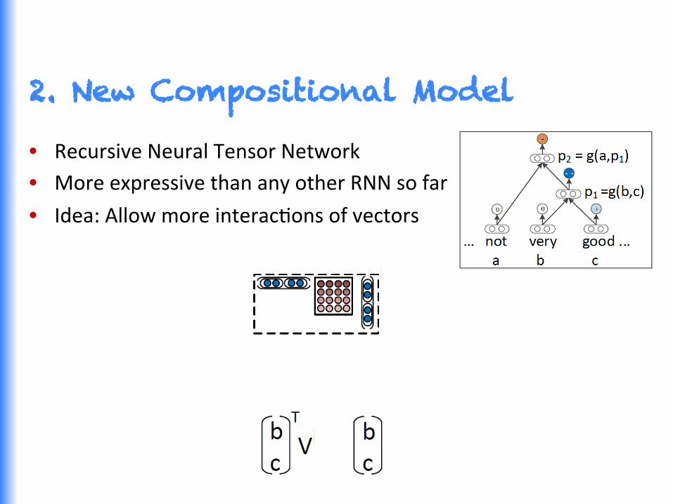
2. New Compositional Model
• Recursive Neural Tensor Network • More expressive than any other RNN so far
• Idea: Allow more interacGons of vectors

2. New Compositional Model
• Recursive Neural Tensor Network
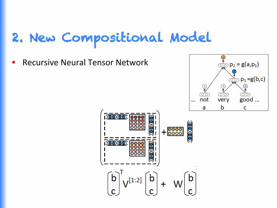
2. New Compositional Model
• Recursive Neural Tensor Network

Recursive Neural Tensor Network

Experimental Result on Treebank

Experimental Result on Treebank • RNTN can capture X but Y • RNTN accuracy of 72%, compared to MV-‐RNN (65),
biNB (58) and RNN (54)

Negation Results
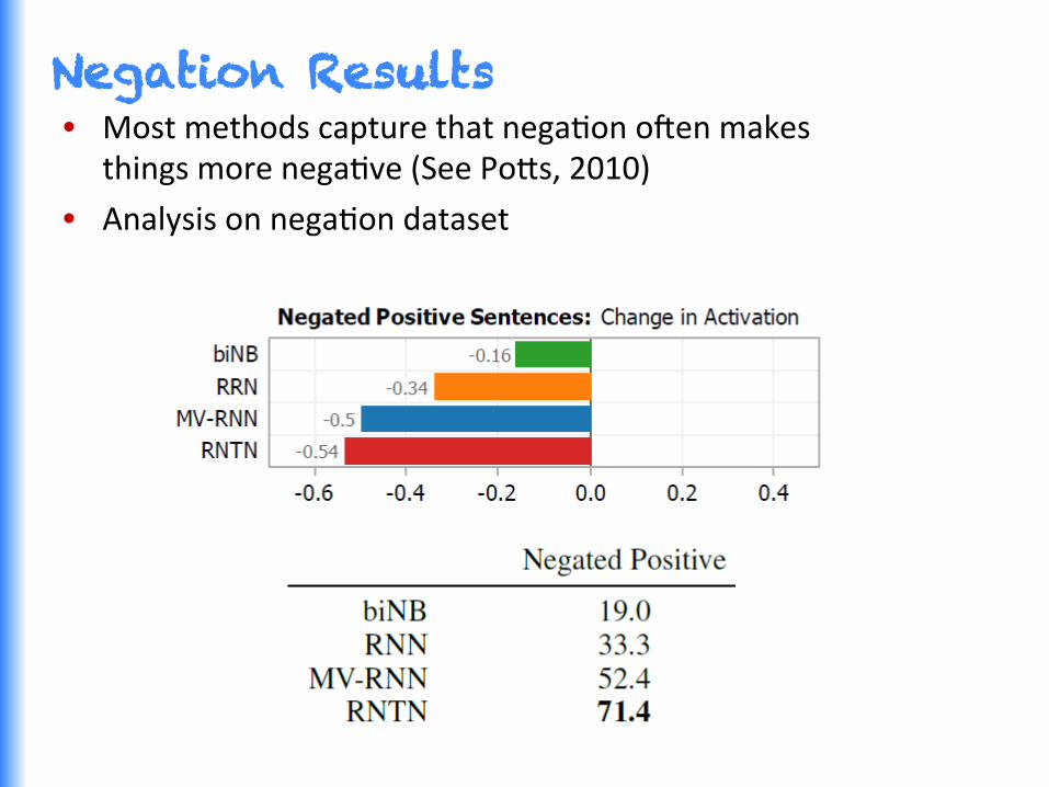
Negation Results • Most methods capture that negaGon o^en makes
things more negaGve (See Po0s, 2010)
• Analysis on negaGon dataset

Negation Results • But how about negaGng negaGves? • PosiGve acGvaGon should increase!

Visualizing Deep Learning: Word Embeddings

Overview of RNN Model Variations • ObjecGve FuncGons
• Supervised Scores for Structure Predic@on • Classifier for Sen@ment, Rela@ons, Visual Objects, Logic
• Unsupervised autoencoding immediate children or enGre tree structure
• ComposiGon FuncGons
• Syntac@cally-‐Un@ed Weights
• Matrix Vector RNN • Tensor-‐Based Models
• Tree Structures
• Cons@tuency Parse Trees • Combinatory Categorical Grammar Trees
• Dependency Parse Trees • Fixed Tree Structures (ConnecGons to CNNs)
162

Summary: Recursive Deep Learning • Recursive Deep Learning can predict hierarchical structure and classify the
structured output using composiGonal vectors • State-‐of-‐the-‐art performance (all with code on www.socher.org)
• Parsing on the WSJ (Java code soon) • Sen@ment Analysis on mulGple corpora • Paraphrase detec@on with unsupervised RNNs • Rela@on Classifica@on on SemEval 2011, Task8 • Object detec@on on Stanford background and MSRC datasets
163
Features
Grass Tree
Segments
A small crowd quietly enters the historic church
historicthe
quietly enters
SVP
Det. Adj.
NP
Semantic Representations
VP
A small crowd
NP
NP
church
N.
People Building
IndicesWords
Semantic Representations
Parsing Natural Language SentencesParsing Natural Language Sentences
Parsing Natural Scene ImagesParsing Natural Scene Images

Part 3
1. Assorted Speech and NLP ApplicaGons 2. Deep Learning: General Strategy and Tricks 3. Resources (readings, code, …) 4. Discussion
164
Assorted Speech and NLP Applications
Part 3.1: ApplicaGons
165

Existing NLP Applications
• Language Modeling (Speech RecogniGon, Machine TranslaGon) • Word-‐Sense Learning and DisambiguaGon
• Reasoning over Knowledge Bases • AcousGc Modeling
• Part-‐Of-‐Speech Tagging • Chunking • Named EnGty RecogniGon
• SemanGc Role Labeling • Parsing • SenGment Analysis • Paraphrasing • QuesGon-‐Answering 166

Language Modeling
• Predict P(next word | previous word)
• Gives a probability for a longer sequence
• ApplicaGons to Speech, TranslaGon and Compression
• ComputaGonal bo0leneck: large vocabulary V means that compuGng the output costs #hidden units x |V|.
167

Neural Language Model
• Bengio et al NIPS’2000 and JMLR 2003 “A Neural Probabilis<c Language Model” • Each word represented by a distributed conGnuous-‐valued code
• Generalizes to sequences of words that are semanGcally similar to training sequences
168

Recurrent Neural Net Language Modeling for ASR
• [Mikolov et al 2011] Bigger is be0er… experiments on Broadcast News NIST-‐RT04
perplexity goes from 140 to 102
Paper shows how to train a recurrent neural net with a single core in a few days, with > 1% absolute improvement in WER
Code: http://www.fit.vutbr.cz/~imikolov/rnnlm/!
Code: h0p://www.fit.vutbr.cz/~imikolov/rnnlm/
169

Application to Statistical Machine Translation
• Schwenk (NAACL 2012 workshop on the future of LM) • 41M words, Arabic/English bitexts + 151M English from LDC
• Perplexity down from 71.1 (6 Gig back-‐off) to 56.9 (neural model, 500M memory)
• +1.8 BLEU score (50.75 to 52.28)
• Can take advantage of longer contexts
• Code: http://lium.univ-lemans.fr/cslm/!
170

Learning Multiple Word Vectors
• Tackles problems with polysemous words
• Can be done with both standard �-‐idf based methods [Reisinger and Mooney, NAACL 2010]
• Recent neural word vector model by [Huang et al. ACL 2012] learns mulGple prototypes using both local and global context
• State of the art correlaGons with human similarity judgments
171

Learning Multiple Word Vectors • VisualizaGon of learned word vectors from
Huang et al. (ACL 2012)
172
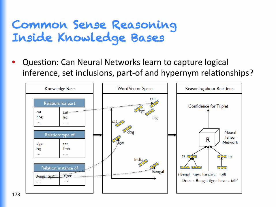
Common Sense Reasoning Inside Knowledge Bases
• QuesGon: Can Neural Networks learn to capture logical inference, set inclusions, part-‐of and hypernym relaGonships?
173

Neural Networks for Reasoning over Relationships
• Higher scores for each triplet T = (e1,R,e2) indicate that enGGes are more likely in relaGonship
• Training uses contrasGve esGmaGon funcGon, similar to word vector learning
• NTN scoring funcGon:
• Cost: 174

Accuracy of Predicting True and False Relationships
• Related Work • Bordes, Weston,
Collobert & Bengio, AAAI 2011)
• (Bordes, Glorot, Weston & Bengio, AISTATS 2012)
175
Model FreeBase WordNet
Distance Model 68.3 61.0
Hadamard Model 80.0 68.8
Standard Layer Model (<NTN) 76.0 85.3
Bilinear Model (<NTN) 84.1 87.7
Neural Tensor Network (Chen et al. 2013) 86.2 90.0

Accuracy Per Relationship
176

Deep Learning General Strategy and Tricks
Part 3.2
177

General Strategy 1. Select network structure appropriate for problem
1. Structure: Single words, fixed windows vs Recursive Sentence Based vs Bag of words
2. Nonlinearity 2. Check for implementaGon bugs with gradient checks
3. Parameter iniGalizaGon 4. OpGmizaGon tricks
5. Check if the model is powerful enough to overfit 1. If not, change model structure or make model “larger”
2. If you can overfit: Regularize
178

Non-linearities: What’s used
logisGc (“sigmoid”) tanh
tanh is just a rescaled and shi^ed sigmoid
tanh is what is most used and o^en performs best for deep nets
tanh(z) = 2logistic(2z)−1
179

Non-linearities: There are various other choices
hard tanh so^ sign recGfier
• hard tanh similar but computaGonally cheaper than tanh and saturates hard.
• [Glorot and Bengio AISTATS 2010, 2011] discuss so^sign and recGfier
rect(z) =max(z, 0)softsign(z) = a1+ a
180
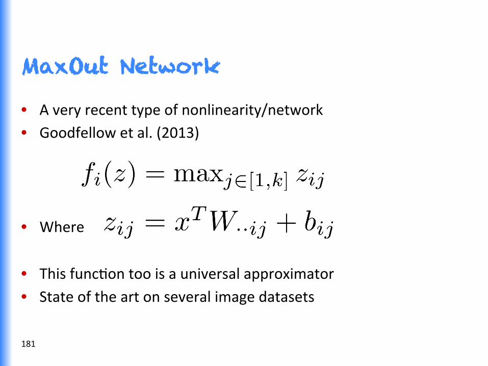
MaxOut Network
• A very recent type of nonlinearity/network • Goodfellow et al. (2013)
• Where
• This funcGon too is a universal approximator • State of the art on several image datasets
181

Gradient Checks are Awesome!
• Allows you to know that there are no bugs in your neural network implementaGon!
• Steps: 1. Implement your gradient 2. Implement a finite difference computaGon by looping
through the parameters of your network, adding and subtracGng a small epsilon (~10^-‐4) and esGmate derivaGves
3. Compare the two and make sure they are the same 182
,

General Strategy 1. Select appropriate Network Structure
1. Structure: Single words, fixed windows vs Recursive Sentence Based vs Bag of words
2. Nonlinearity 2. Check for implementaGon bugs with gradient check
3. Parameter iniGalizaGon 4. OpGmizaGon tricks
5. Check if the model is powerful enough to overfit 1. If not, change model structure or make model “larger”
2. If you can overfit: Regularize
183

Parameter Initialization
• IniGalize hidden layer biases to 0 and output (or reconstrucGon) biases to opGmal value if weights were 0 (e.g. mean target or inverse sigmoid of mean target).
• IniGalize weights ~ Uniform(-‐r,r), r inversely proporGonal to fan-‐in (previous layer size) and fan-‐out (next layer size):
for tanh units, and 4x bigger for sigmoid units [Glorot AISTATS 2010]
• Pre-‐training with Restricted Boltzmann machines
184

• Gradient descent uses total gradient over all examples per update, SGD updates a^er only 1 or few examples:
• L = loss funcGon, zt = current example, θ = parameter vector, and εt = learning rate.
• Ordinary gradient descent as a batch method, very slow, should never be used. Use 2nd order batch method such as LBFGS. On large datasets, SGD usually wins over all batch methods. On smaller datasets LBFGS or Conjugate Gradients win. Large-‐batch LBFGS extends the reach of LBFGS [Le et al ICML’2011].
Stochastic Gradient Descent (SGD)
185

Learning Rates
• Simplest recipe: keep it fixed and use the same for all parameters.
• Collobert scales them by the inverse of square root of the fan-‐in of each neuron
• Be0er results can generally be obtained by allowing learning rates to decrease, typically in O(1/t) because of theoreGcal convergence guarantees, e.g., with hyper-‐parameters ε0 and τ
• Be0er yet: No learning rates by using L-‐BFGS or AdaGrad (Duchi et al. 2011)
186

Long-Term Dependencies and Clipping Trick
• In very deep networks such as recurrent networks (or possibly recursive ones), the gradient is a product of Jacobian matrices, each associated with a step in the forward computaGon. This can become very small or very large quickly [Bengio et al 1994], and the locality assumpGon of gradient descent breaks down.
• The soluGon first introduced by Mikolov is to clip gradients to a maximum value. Makes a big difference in RNNs
187
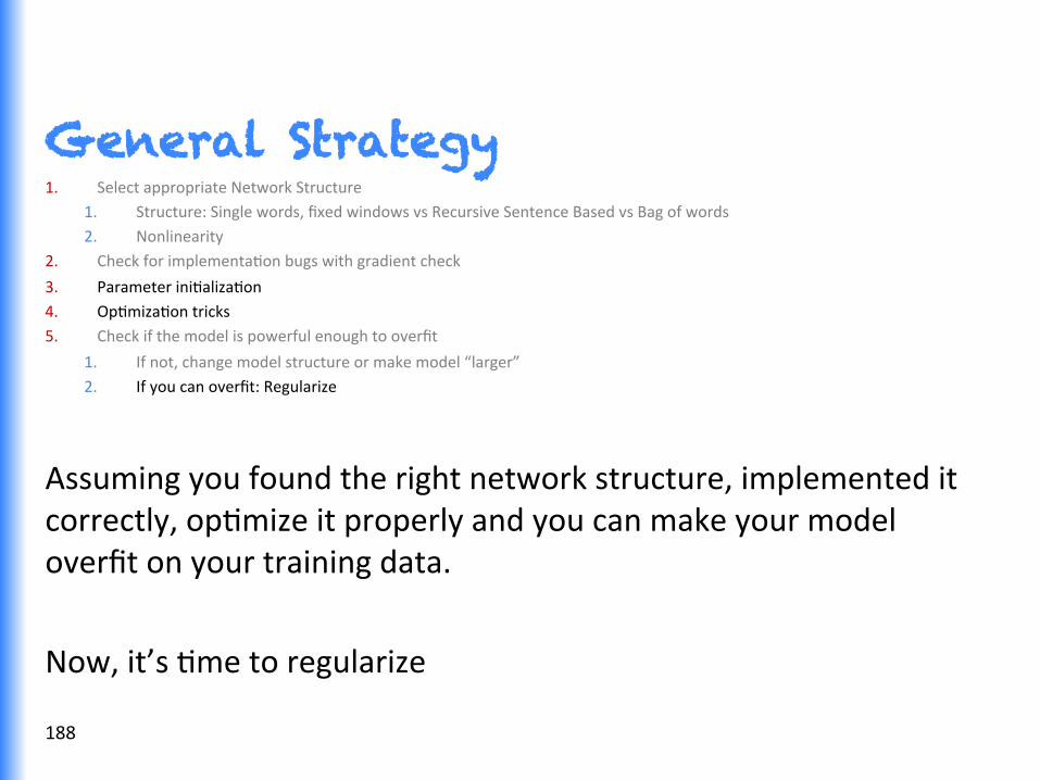
General Strategy 1. Select appropriate Network Structure
1. Structure: Single words, fixed windows vs Recursive Sentence Based vs Bag of words 2. Nonlinearity
2. Check for implementaGon bugs with gradient check
3. Parameter iniGalizaGon 4. OpGmizaGon tricks 5. Check if the model is powerful enough to overfit
1. If not, change model structure or make model “larger” 2. If you can overfit: Regularize
Assuming you found the right network structure, implemented it correctly, opGmize it properly and you can make your model overfit on your training data.
Now, it’s Gme to regularize
188

Prevent Overfitting: Model Size and Regularization
• Simple first step: Reduce model size by lower number of units and layers and other parameters
• Standard L1 or L2 regularizaGon on weights • Early Stopping: Use parameters that gave best validaGon error • Sparsity constraints on hidden acGvaGons, e.g. add to cost:
• Dropout (Hinton et al. 2012): • Randomly set 50% of the inputs at each layer to 0
• At test Gme half the outgoing weights (now twice as many)
• Prevents Co-‐adaptaGon 189

Deep Learning Tricks of the Trade • Y. Bengio (2012), “PracGcal RecommendaGons for Gradient-‐
Based Training of Deep Architectures”
• Unsupervised pre-‐training • StochasGc gradient descent and se�ng learning rates • Main hyper-‐parameters • Learning rate schedule & early stopping • Minibatches • Parameter iniGalizaGon • Number of hidden units • L1 or L2 weight decay • Sparsity regularizaGon
• Debugging à Finite difference gradient check (Yay) • How to efficiently search for hyper-‐parameter configuraGons
190

Resources: Tutorials and Code Part 3.3: Resources
191

Related Tutorials • See “Neural Net Language Models” Scholarpedia entry • Deep Learning tutorials: h0p://deeplearning.net/tutorials • Stanford deep learning tutorials with simple programming
assignments and reading list h0p://deeplearning.stanford.edu/wiki/
• Recursive Autoencoder class project h0p://cseweb.ucsd.edu/~elkan/250B/learningmeaning.pdf
• Graduate Summer School: Deep Learning, Feature Learning h0p://www.ipam.ucla.edu/programs/gss2012/
• ICML 2012 RepresentaGon Learning tutorial h0p://www.iro.umontreal.ca/~bengioy/talks/deep-‐learning-‐tutorial-‐2012.html
• More reading (including tutorial references): hjp://nlp.stanford.edu/courses/NAACL2013/
192

Software
• Theano (Python CPU/GPU) mathemaGcal and deep learning library h0p://deeplearning.net/so^ware/theano
• Can do automaGc, symbolic differenGaGon • Senna: POS, Chunking, NER, SRL
• by Collobert et al. h0p://ronan.collobert.com/senna/ • State-‐of-‐the-‐art performance on many tasks • 3500 lines of C, extremely fast and using very li0le memory
• Recurrent Neural Network Language Model h0p://www.fit.vutbr.cz/~imikolov/rnnlm/
• Recursive Neural Net and RAE models for paraphrase detecGon, senGment analysis, relaGon classificaGon www.socher.org
193

Software: what’s next
• Off-‐the-‐shelf SVM packages are useful to researchers from a wide variety of fields (no need to understand RKHS).
• One of the goals of deep learning: Build off-‐the-‐shelf NLP classificaGon packages that are using as training input only raw text (instead of features) possibly with a label.
194

Discussion Part 3.4:
195
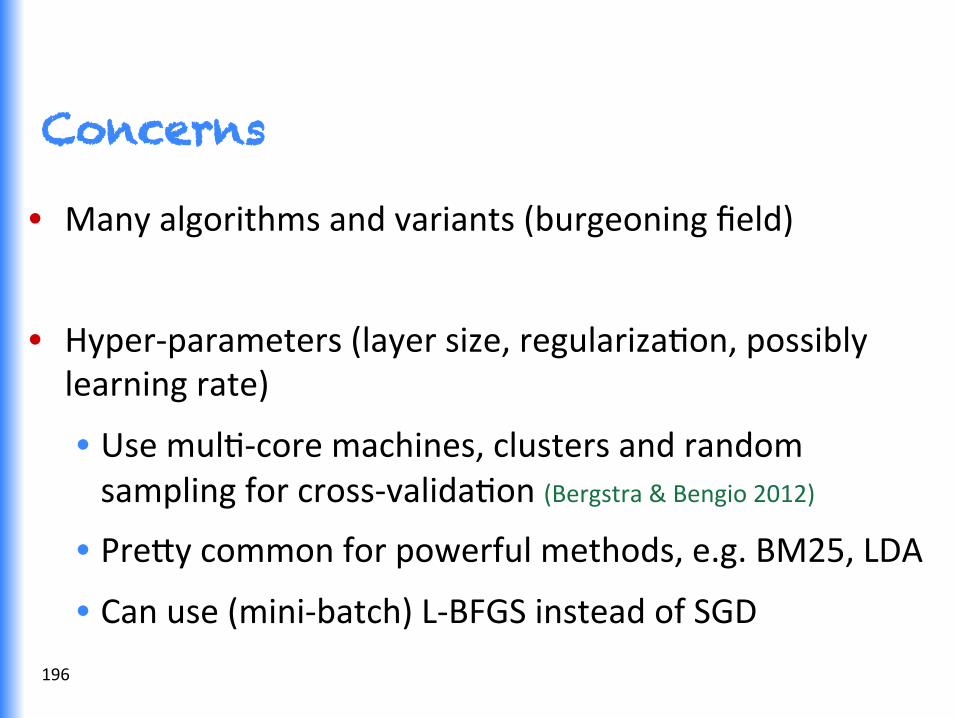
Concerns
• Many algorithms and variants (burgeoning field)
• Hyper-‐parameters (layer size, regularizaGon, possibly learning rate)
• Use mulG-‐core machines, clusters and random sampling for cross-‐validaGon (Bergstra & Bengio 2012)
• Pre0y common for powerful methods, e.g. BM25, LDA
• Can use (mini-‐batch) L-‐BFGS instead of SGD
196

Concerns
• Not always obvious how to combine with exisGng NLP
• Simple: Add word or phrase vectors as features. Gets close to state of the art for NER, [Turian et al, ACL 2010]
• Integrate with known problem structures: Recursive and recurrent networks for trees and chains
• Your research here
197

Concerns
• Slower to train than linear models
• Only by a small constant factor, and much more compact than non-‐parametric (e.g. n-‐gram models)
• Very fast during inference/test Gme (feed-‐forward pass is just a few matrix mulGplies)
• Need more training data
• Can handle and benefit from more training data, suitable for age of Big Data (Google trains neural nets with a billion connecGons, [Le et al, ICML 2012])
198

Concerns
• There aren’t many good ways to encode prior knowledge about the structure of language into deep learning models • There is some truth to this. However:
• You can choose architectures suitable for a problem domain, as we did for linguisGc structure
• You can include human-‐designed features in the first layer, just like for a linear model • And the goal is to get the machine doing the learning!
199
Concern: Problems with model interpretability
• No discrete categories or words, everything is a conGnuous vector. We’d like have symbolic features like NP, VP, etc. and see why their combinaGon makes sense.
• True, but most of language is fuzzy and many words have so^ relaGonships to each other. Also, many NLP features are already not human-‐understandable (e.g., concatenaGons/combinaGons of different features).
• Can try by projecGons of weights and nearest neighbors, see part 2
200

Concern: non-convex optimization
• Can iniGalize system with convex learner • Convex SVM
• Fixed feature space
• Then opGmize non-‐convex variant (add and tune learned features), can’t be worse than convex learner
• Not a big problem in pracGce (o^en relaGvely stable performance across different local opGma)
201

Advantages
• Despite a small community in the intersecGon of deep learning and NLP, already many state of the art results on a variety of language tasks
• O^en very simple matrix derivaGves (backprop) for training and matrix mulGplicaGons for tesGng à fast implementaGon
• Fast inference and well suited for mulG-‐core CPUs/GPUs and parallelizaGon across machines
202
Learning Multiple Levels of Abstraction
• The big payoff of deep learning is to learn feature representaGons and higher levels of abstracGon
• This allows much easier generalizaGon and transfer between domains, languages, and tasks
203

The End
204