so you want to use a real equation of state · so you want to use a "real" equation of...

Operated by Los Alamos National Security, LLC for the U.S. Department of Energy’s NNSA

U N C L A S S I F I E D

LA-UR 10-07860


U N C L A S S I F I E D Slide 1

So you want to use a "real" equation of state

Presented at the Department of Applied Mathematics and Statistics Colloquium

Stony Brook University Stony Brook, NY

John W. Grove CCS-2: Computational Physics

Computer, Computational, and Statistical Sciences Division Los Alamos National Laboratory

P.O. Box 1663, MS D413 Los Alamos National Laboratory Los Alamos, NM 87544

[email protected]



LA-UR 10-07860

Real Equations of State

Some Popular Mythical Creatures

Slide 2

Bigfoot

The Lock Ness Monster

The Abominable Snowman

Unicorns

Genies

Fairies



LA-UR 10-07860

Slide 3

The Equation of State is Where the Rubber Meets the Road

n  The connection of the hydrodynamic equations with real materials is via the EOS •  The abstract conservation laws of mass, momentum, and energy are completely

generic and apply to any flow •  To reproduce the behavior of a real flow requires specifying the relation between

the material stress, internal energy, and material deformation •  For hydrodynamics this reduces to specifying the relation between the specific

internal energy, mass density, and pressure. —  Typically this is done by giving the pressure as a function of density and

specific internal energy:

—  This relation is called an incomplete equation of state and is often sufficient for many applications

—  More generally, the thermodynamics are related via a potential with the temperature, such as a Helmholtz free energy as a function of specific volume and temperature

( ),P P eρ=

( ), , 1 , , F F V T V dF SdT PdV e F TSρ= = = − − = +



LA-UR 10-07860

How a General EOS Enters into a Hydro-code n  The basic ingredients for many hyperbolic solvers include

•  Evaluate the flux •  Compute the eigenvalues and eigenvectors of the flux derivative •  Compute approximations to Riemann problem solutions

n  For hydro these quantities can be expressed in terms of •  Basic thermodynamic quantities

—  Pressure, density, specific internal energy, temperature, and perhaps specific entropy

•  Thermodynamic derivatives —  The Grüneisen exponent:

—  The adiabatic sound speed:

—  The specific heat at constant volume:

—  and/or the specific heat at constant pressure: •  Other thermodynamic expressions may be useful, but any thermodynamic

derivative can be expressed in terms of these quantities

n  Expressing the operations in a solver in terms of these quantities is a first step in modifying a code to support a general equation of state

Slide 4

1 Pe ρρ

∂Γ = ∂2

S e

P P Pc ρ ρ ρ∂ ∂= = +Γ∂ ∂

VV

eC T∂= ∂ ( )

PP P

P

e PVS hC T T T T∂ +∂ ∂= = =∂ ∂ ∂



LA-UR 10-07860

Hyperbolic Systems of Conservation Laws and the Ingredients of Flow Solvers

n  Partial differential equations in divergence form:

n  Hyperbolic: has all real eigenvalues and a complete set of eigenvectors for every spatial direction n.

n  The integral form of these equations form the basis for virtually all numerical solvers:

n  Basically all finite volume type solvers seek to time advance the solution by estimating the integral of the flux over the boundary of the region.

n  A key technique used in estimating the flux integrals is the characteristic form of the equation which for one spatial dimension can be written as:

Slide 5

( )1, , ,t n+∇ = =u F S F F Fr rg K

( ), dd

= FA u n nu

rg

( ) ( ) ( ) ( ) ( ) ( )

( )

,

fixedt t t t t t

d ddV dA SdV dV dA SdVdt dt

t

Ω ∂Ω Ω Ω ∂Ω Ω

+ = + + =

= Ω

∫ ∫ ∫ ∫ ∫ ∫u n F u un b n F

b

r rg g g

boundary velocity of the moving body

[ ] , t xdd

λ λ+ = =Fl u u lS l lu



LA-UR 10-07860

How the Equation of State Enters into Hydro

n  For simplicity we will only discuss inviscid hydrodynamics

n  The Euler equations describing the laws of conservation of mass, momentum, and energy for a conservation system:

n  The equation of state is required to evaluate the flux F

n  Extensions to include material strength, viscosity, thermal conduction, mixtures, mass diffusion, and radiative transport introduce additional constitutive equations that often will require additional equation of state information, in particular the thermodynamic temperature.

Slide 6

2 2

0, , ,

1 12 2

Tt P

u e u e P

ρ ρρ ρ ρ

ρρ ρ

⎛ ⎞ ⎛ ⎞⎜ ⎟ ⎜ ⎟ ⎛ ⎞⎜ ⎟ ⎜ ⎟ ⎜ ⎟⎜ ⎟ ⎜ ⎟+∇ = = = + = ⎜ ⎟⎜ ⎟ ⎜ ⎟ ⎜ ⎟⎛ ⎞ ⎛ ⎞ ⎝ ⎠⎜ ⎟ ⎜ ⎟+ + +⎜ ⎟ ⎜ ⎟⎜ ⎟ ⎜ ⎟⎝ ⎠ ⎝ ⎠⎝ ⎠ ⎝ ⎠

uw F S w u F u u I S g

u gu u

gg



LA-UR 10-07860

Characteristics Analysis Deepens the EOS Usage

n  A fundamental tool in designing hydrodynamic solvers is the characteristic analysis of the Euler equations

n  For simplicity we restrict our attention to one spatial dimension flows and ignore body forces, for smooth flow the equation becomes

n  This form introduces the specific entropy S into the flow equations, which is an equation of state function of say the specific internal energy and density

n  One can rewrite the above equation in characteristic form by introducing the sound speed c:

Slide 7

1, 0, 0, 0D D u Du P DS De uu PDt t x Dt x Dt x Dt Dt x

ρ ρρ

∂ ∂ ∂ ∂ ∂= + + = + = = + =∂ ∂ ∂ ∂ ∂

( ) ( ) 20, 0, S

P P u u S S Pu c c u c u ct x t x t x

ρρ

∂ ∂ ∂ ∂ ∂ ∂ ∂⎡ ⎤ ⎡ ⎤+ ± ± + ± = + = =⎢ ⎥ ⎢ ⎥∂ ∂ ∂ ∂ ∂ ∂ ∂⎣ ⎦ ⎣ ⎦



LA-UR 10-07860

A Little More on Characteristics n  Entropy is not usually a very convenient variable to use

for hydro solvers •  Often it is not easily available and might even require significant computational overhead

to compute

n  Most commonly we desire an expression in terms of functions of density and specific internal energy. The characteristic equations can be written in terms of these two quantities as:

n  This form, which is probably the most commonly used version in hydro-solvers, introduces another EOS quantity, the Grüneisen exponent Γ.

n  When temperature is needed one more EOS quantity enters, the specific heat at constant volume CV:

Slide 8

( ) ( )

2

2 2

,

, , 0, , 0, 0

P PdP c d dee

Pc c u u c u P u u ut x t xe e e e

ρ

ρ ρρ

ρ ρ ρ ρρ ρ ρ

ρ

⎛ ⎞ ∂= −Γ + Γ Γ =⎜ ⎟ ∂⎝ ⎠⎡ ⎤ ⎡ ⎤⎛ ⎞ ⎛ ⎞ ⎛ ⎞ ⎛ ⎞

⎛ ⎞⎛ ⎞ ∂ ∂ ∂ ∂⎢ ⎥ ⎢ ⎥⎜ ⎟ ⎜ ⎟ ⎜ ⎟ ⎜ ⎟−Γ ± Γ + ± = − + =⎜ ⎟⎜ ⎟ ⎢ ⎥ ⎢ ⎥⎜ ⎟ ⎜ ⎟ ⎜ ⎟ ⎜ ⎟∂ ∂ ∂ ∂⎝ ⎠⎝ ⎠ ⎜ ⎟ ⎜ ⎟ ⎜ ⎟ ⎜ ⎟⎢ ⎥ ⎢ ⎥⎝ ⎠ ⎝ ⎠ ⎝ ⎠ ⎝ ⎠⎣ ⎦ ⎣ ⎦

VV

e CT∂ =∂



LA-UR 10-07860

Basic Steps in Hydro Solvers n  Most modern hydro solvers use a combination of calculations to

advance the solution in time n  Reconstruction: Given cell average quantities construct a continuous function that

recovers these averages •  Generally applied to some select set of fields such as density, specific internal energy (or often

pressure), and velocities •  Other fields are then computed using the equation of state to evaluate their values or perhaps

their slope

n  Godunov type schemes compute approximate solutions to Riemann problems across cell faces •  Linear approximate Riemann problem solvers use the characteristic eigenvectors •  Exact solvers require evaluating the Hugoniot and adiabatic waves curves:

n  Semi-discrete formulations also will include Runga-Kutta or other types of integrations for the time derivatives of the flow state in terms of the discretized fluxes, whose evaluations may require additional EOS information.

Slide 9

( ) ( ) ( ) ( ) ( )( ) ( ) ( )

( ) ( )( )

0

0 00 0 0 0 0 0 0 0

0 0 0 0 0

0

0

, ,, , , , , 0, , ,

2

, , ,

,

ah a a a

h

P

PS

P V e P V e dee e V V V V P V e P V e V e V e V V P V edV

P P V V P V e P Pu u dP P P

cρ

+− = − ⇒ = + = = ⇒ =

⎧ − − ≥⎪⎪= ± ⎨

<⎪⎪⎩

∫



LA-UR 10-07860

Slide 10

Equations of State 101 n  The equation of state is what connects the “physical” properties of a

material to the hydrodynamic equations

n  Closes the Euler equations for conservation of mass, momentum, and energy by providing a pressure that can be computed as a function of density and energy (or equivalent).

n  In terms of general thermodynamics, the equation of state is defined by a free energy and its derivatives •  Specific Helmholtz free energy: •  Specific internal energy: •  Specific Enthalpy: •  Specific Gibb’s free energy:

n  The existence of a free energy ensures that the thermodynamics has a well defined entropy

( ) = − −, , F V T dF PdV SdT( ) = − +, , E V S dE PdV TdS

( ) = +, , H P S dH VdP TdS( ) = −, , G P T dG VdP SdT



LA-UR 10-07860

Equations of State 101: Free Energy Constraints

n  Equilibrium thermodynamics constrains convexity of the free energies •  The Helmholtz free energy is separately convex in specific volume and

temperature •  The specific internal energy is jointly convex in specific volume and specific entropy •  The specific enthalpy free energy is concave in pressure and convex in specific

entropy •  The Gibb’s free energy is jointly concave in pressure and temperature

n  These conditions ensure that the sound speed for the material is real (non-negative bulk modulus) and that the specific heats are non-negative

n  We also assume non-negative specific volume (density), and temperature •  Note: we need not assume non-negative pressure and thus allow for materials in

tension —  However in reality such states on only meta-stable

•  This can raise several issues for hydro solvers

Slide 11



LA-UR 10-07860

Equations of State 101: Relations Between Free Energies

n  The free energies are related to one another via Legendre transformations:

n  See the reference: “The Riemann Problem for Fluid Flow of Real Materials”, R. Menikoff and B. Plohr, Rev. Mod. Phys., Vol. 61, no. 1, 1989. Or your favorite book on thermodynamics for more details.

Slide 12

( ) ( ) ( ) ( )

( ) ( ) ( ) ( )

( ) ( ) ( ) ( )

( ) ( ) ( ) ( )

( ) ( ) ( )

⎡ ⎤ ⎡ ⎤= + = −⎣ ⎦ ⎣ ⎦

⎡ ⎤ ⎡ ⎤= + = −⎣ ⎦ ⎣ ⎦

⎡ ⎤ ⎡ ⎤= + = −⎣ ⎦ ⎣ ⎦

⎡ ⎤ ⎡ ⎤= − = +⎣ ⎦ ⎣ ⎦

⎡ ⎤= − + =⎣ ⎦,

, sup , , , inf ,

, inf , , , sup ,

, inf , , , sup ,

, sup , , , inf ,

, inf , , ,

ST

V P

V P

ST

V S

E V S F V T TS F V T E V S TS

G P T F V T PV F V T F V S PV

H P S E V S PV E V S H P S PV

H P S G P T TS G P T H P S TS

G P T E V S TS PV E V S ( )

( ) ( ) ( ) ( )

⎡ ⎤+ −⎣ ⎦

⎡ ⎤ ⎡ ⎤⎡ ⎤ ⎡ ⎤= + + = − −⎣ ⎦ ⎣ ⎦⎢ ⎥ ⎣ ⎦⎣ ⎦

,sup ,

, inf sup , , , sup inf ,

P T

V ST P

G P T TS PV

H P S F V T PV TS F V T F V S PV TS



LA-UR 10-07860

“Observables” and EOS Free Energies n  The “measurable” quantities of interest for an equation of state include n  Specific Heats

•  CV = specific heat at constant volume: —  Often taken as constant for analytic

EOS’s •  CP = specific heat at constant pressure:

—  Is a quantity that is experimentally measurable

•  Thermodynamic stability requires CP ≥ CV ≥ 0

n  Compressibilities: •  KT = isothermal compressibility: •  = isothermal bulk modulus

cT = isothermal sound speed •  KS = isentropic compressibility: •  = isentropic (adiabatic) bulk modulus •  c = isentropic (adiabatic) sound speed •  Thermodynamic stability requires KT ≥ KS ≥ 0

Slide 13

∂ ∂ ∂≡ = = −

∂ ∂ ∂

2

2VV V

S E FC T T

T T T

∂ ∂ ∂≡ = = −

∂ ∂ ∂

2

2PP P

S H GC T T

T T T

ρ∂ ∂ ∂

≡ − = = −∂ ∂ ∂

=2

2 21 1 1 1

TT T T

V F GK

V P PV P V P cρ 2Tc

ρ∂ ∂ ∂

≡ − = = −∂ ∂ ∂

=2

2 21 1 1 1

SS T

V E HK

V P PV P V P cρ 2c



LA-UR 10-07860

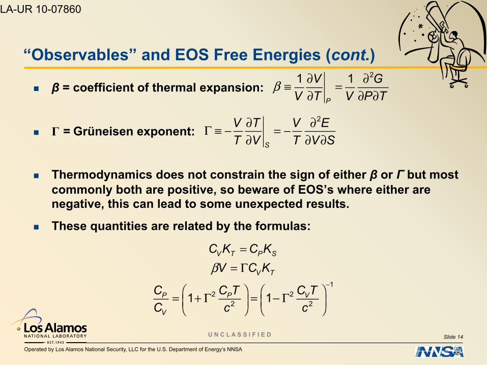
“Observables” and EOS Free Energies (cont.)

n  β = coefficient of thermal expansion:

n  Γ = Grüneisen exponent:

n  Thermodynamics does not constrain the sign of either β or Γ but most commonly both are positive, so beware of EOS’s where either are negative, this can lead to some unexpected results.

n  These quantities are related by the formulas:

Slide 14

β ∂ ∂≡ =∂ ∂ ∂

21 1

P

V GV T V P T

∂ ∂Γ ≡ − = −∂ ∂ ∂

2

S

V T V ET V T V S

β−

== Γ

⎛ ⎞ ⎛ ⎞= + Γ = − Γ⎜ ⎟ ⎜ ⎟⎝ ⎠ ⎝ ⎠

12 2

2 21 1

V T P S

V T

P P V

V

C K C KV C K

C C T C TC c c



LA-UR 10-07860

n  Many “real” (i.e. not perfect gases) are of the Grüneisen form:

n  The temperature is constrained by the incomplete EOS via the relations: •  Scalar hyperbolic equation whose characteristics are the constant entropy curves

of the incomplete EOS. •  The temperature can then be determined from any temperature data on a non-

isentropic curve in energy-specific volume space

•  Commonly we assume a constant specific heat at constant volume: —  For Grüneisen form EOS’s the temperature can be computed by solving the

ordinary linear differential equation:

11( , ), PP T T P TT TP P V e de TdS PdV dS de dV P T

T T V e V e e V

∂ ∂ ∂ ∂ ∂= = − ⇒ = + ⇒ = ⇒ − = − = − Γ∂ ∂ ∂ ∂ ∂

Some Real EOS Examples

Slide 15

( ) ( ) ( )( )r r

Ve e V P P V

VΓ

− = −

VV

SC TT∂≡∂

( ) ( )( ), r rr V r V r r

dT dee e V C T T V C T PdV V dV

Γ⎡ ⎤− = − + = +⎢ ⎥⎣ ⎦



LA-UR 10-07860

EOS Examples

n  Stiff gamma law gas: •  Simple analytic EOS is easy to implement •  Very useful in algorithm development since it can be used to

add stiffness to the EOS thus stressing the hydrodynamic solver •  Also useful to approximate more complicated EOS’s in limited domains •  Domain consists of V > 0 and P > -P∞

n  JWL (Jones-Wilkins-Lee) equation of state: •  Simple exponential reference curve makes implementation relatively easy •  Often used to model detonation products •  Large database of parameter values is available from the LLNL HE reference web

site (registration required)

Slide 16

( )( )1 , VP P V e e C T PV∞ ∞+ Γ+ =Γ = +

( ) ( )( )

( ) ( ) ( ) ( ) ( )

1 2

1 21 2

1 2

01 2 0

1 1 ,

, , , ,

RV R Vr V r

RV R VRV R V

r r r r r

P e A e B e e e V C T T VV RV R V

e e VP V Ae Be e V A B e V P V T V TR R V

ω

ω ω ω

ω

− −

−− −− −

⎛ ⎞ ⎛ ⎞= + − + − − = −⎜ ⎟ ⎜ ⎟

⎝ ⎠ ⎝ ⎠

⎛ ⎞′Γ = = + = + = − = ⎜ ⎟⎝ ⎠



LA-UR 10-07860

EOS Examples: Steinberg-Mie-Grüneisen Equation of State

n  Grüneisen exponent is linear in specific volume:

n  Reference Hugoniot formulation (linear Us-Up at constant volume):

n  Energy and pressure are related by a Hugoniot equation:

n  Pressure reference is a rational function of specific volume:

n  Defined for compression V≤V0 •  Extensions to expansion generally use a stiff gamma law form •  This introduces a discontinuity in the EOS at the reference density that can impact the solver.

n  Commonly used to model metals as part of an elastic-plastic constitutive model •  But is used in many other contexts as well, e.g. unburned high explosives

n  Has a complicated formula for the adiabatic and isothermal sound speeds •  EOS evaluation much more expensive •  Determining whether an evaluation stays in the EOS domain (positive isothermal bulk modulus) can be difficult

Slide 17

00 0

1V VbV V

⎛ ⎞Γ = Γ + −⎜ ⎟

⎝ ⎠

( ) ( ) 2 00 1 2 3

0

, ,s pV VU c S U S S S SV

ξ ξ ξ ξ ξ −= + = + + =

( ) ( ) ( )00 02

rr

P V Pe V e V V

+= + −

( )( )

2 00 0 0 2

0

, 1

rV VP V P cVS

ξρ ξξ ξ

−= + =−⎡ ⎤⎣ ⎦



LA-UR 10-07860

More Sophisticated EOS Models n  Elements and simple compounds are often

modeled using electron structure methods, see for example: •  S. Eliezer, A. Ghatak and H. Hora, Fundamentals of

Equations of State. (World Scientific Publishing Co. Ptc. Ltd., Singapore, 2002)

•  R. B. Bird, W. E. Stewart and E. N. Lightfoot, Transport Phenomena, Second Edition ed. (John Wiley and Sons, New York, NY, 2007).

n  Plastics and polymers EOS models are usually phenomenological and use a variety of methods

n  All of these models try to use the best (or any) experimental data available to calibrate their parameters and may require a numerical integration to compute the appropriate free energy •  However material property data may be few and far

between —  Hugoniot data for solids —  Diamond anvil data for quasi-static responses

•  Dynamic thermal data are difficult to obtain experimentally

Slide 18



LA-UR 10-07860

Tabular Equations of State n  Pre-computes equation of state data and saves it in a tabular format

•  Most commonly as pressure and specific internal energy matrices as functions of density and temperature

•  Examples include the Los Alamos SESAME database and the Lawrence Livermore National Laboratory LEOS tool

•  Some applications take tables of this type and invert them into pressure-temperature based tables —  This is convenient when evaluating pressure-temperature equilibrium mixtures since the

solution method requires frequent EOS evaluations at pressure-temperature points as part of the root finder

n  Allows for the use of arbitrarily complicated (and realistic) EOS models in a format that hides the specific issues of the EOS model from the hydro code •  Well almost!!

n  Evaluation at off-table points is traditionally done by interpolation •  Bilinear is fast, but may not be very accurate •  Rational interpolation methods are generally better for computing off table values but

are more expensive •  Both methods are only C0 in pressure and energy and introduce discontinuities into the

derived fields across mesh boundaries

Slide 19

( ) ( ), , e ,ij i j ij i jP P T e Tρ ρ= =

( ) ( ), , e ,kl k l kl k lP T e P Tρ ρ= =



LA-UR 10-07860

Tabular Equations of State (what lies beneath)

n  Tabular EOS hide a lot of issues that can be of concern to a hydro method n  Thermodynamic derivatives (e.g. sound speeds) may be computed using finite differences

and hence be noisy and inaccurate n  Material phase changes such as melt/vaporization and solid/solid phase changes are

intrinsically discontinuous and introduce difficulties for the evaluation method n  The methods used to derive the original table data may be poorly (or not a all) documented n  The table data may not be thermodynamically consistent

•  Sometimes the models used to derive the EOS data were not consistent in the first place —  Example: tables are often built by using different models in different regions and the overall table data is

not consistent for the reason •  This matters to the hydro since supposedly equivalent EOS formulas can give different results

—  Consider the two formulas for the isentropic bulk modulus:

—  If the EOS is not consistent then these two expressions are not the same and depending on how the code computes the sound speed one may yield a real sound speed and the other an imaginary result.

•  Traditionally when simple artificial finite difference schemes were used the value of the sound speed only mattered in so far as it affect the CFL restricted time step

•  High order Godunov type methods may be much more sensitive to such differences in the way the sound speed is computed and may even fail.

Slide 20

2 2

e V T V

P P P ec V PV V TV e V T

ρ ρ∂ ∂ ∂ ∂= − + = − + Γ∂ ∂ ∂ ∂



LA-UR 10-07860

Tabular Equations of State (what lies beneath … continued)

n  The table data may not be thermodynamically stable •  Thermodynamic stability means:

—  pressure is a non-decreasing function of density at constant temperature (isothermal sound speed is real)

—  specific internal energy is a non-decreasing (preferable increasing) function of temperature for fixed density (CV is non-negative)

•  Often the table contains van-der-Waal loops —  Corresponds to phase changes in the material (typically vaporization) that have both

meta-stable and unstable regions —  Maxwell construction is used to modify the table data to eliminate these loops

•  equivalent to a convexification of the Helmholtz free energy isotherms —  See the previous point about non-consistent data

•  Negative specific heats are completely unphysical so the table data should probably be questioned, but a code will often massage the energy data to force monotonicity.

n  Even “good” data may contain glitches that are manifested in one of the above ways necessitating modifications in the table data •  For example solid-solid phase changes should correspond to flat P-V isotherms, but small

oscillations may have been introduced into the table data due to numerical error.

Slide 21



LA-UR 10-07860

Tabular Equations of State (what lies beneath … we haven’t reached the surface yet) n  Most tables are designed with very large dynamic ranges but it is still

possible that a calculation can exceed the table range •  This is in fact very common at low temperature where the table data tends to be

scarce.

n  How a code treats extrapolations outside of a tables range is an important practical consideration •  Small interpolations outside of the domain that don’t violate stability are usually

okay and provide an important improvement in code robustness

•  Large deviations from the table data are almost assuredly bad and probably should result in a code generated error

•  But will your code check for this or just go merrily along? •  Anecdotally this is one of the most common problems experienced

by users

Slide 22



LA-UR 10-07860

Tabular Equations of State: some practical recommendations (and not just for tables)

n  Developers need to be aware of these issues and design their solvers accordingly

n  Lower order methods may be preferable in some instances when the EOS data is noisy or stiff

n  It is probably a good idea to have the EOS evaluator check for domain violations •  However the extra cost of such checks could degrade code performance, so you may

want to make them optional for production runs where one has a priori confidence that the simulation will stay in a “good” domain

n  Preprocessing tabulated EOS data is probably essential to work around table features and glitches

n  Thermodynamic variable inversions such as creating pressure-temperature tables from other forms can improve code performance for mixtures •  But maybe not for pure materials where you would essentially be inverting the inversion

n  Be prepared to devote a lot of effort to making your EOS interface bug free n  Validation will always be a significant issue that can’t be overlooked.

Slide 23



LA-UR 10-07860

So What’s the Big Deal about Real EOS’s? Knowing the Domain is Critical!

Slide 24

n  Virtually all (all!) models for real equations of state have a finite domain n  The perfect gas EOS is the exception rather than a rule

•  Defined for all positive pressures, densities, specific internal energies

n  When a hydro code gets outside of the domain of the EOS being used unexpected things happen •  If you are lucky your code just crashes

—  E.g. you get an imaginary sound speed and lose hyperbolicity •  More likely it runs (because that is the way you designed it!) but gives an invalid answer

that has nothing to do with reality —  You may be bragging about your great results when some obnoxious person points

out that your solution is completely wrong and unphysical

n  Even when mathematically correct an EOS may at best poorly represent the behavior of a real material outside or a finite range •  Many (most) real equations of state are based on extrapolations off of a limited set of

data —  Mie-Grüneisen models for example are based on an extrapolation off of a reference

Hugoniot and lose validity for flows that deviate very much from the reference values.



LA-UR 10-07860

So What’s the Big Deal about Real EOS’s? They can be expensive!

n  Code performance experience based on simple analytic equations of state (perfect gases) often doesn’t carry over to real EOS. •  The cost of a single EOS evaluation goes from virtually free to a significant fraction of the

solver overhead. •  May even be the dominate cost of the calculation

n  EOS derivatives (e.g. sound speeds) may need to be computed based on finite difference or other approximations. •  This not only adds costs, but can adversely affect high order solvers if the

thermodynamic derivatives are not computed accurately •  Godunov type methods that require Riemann problem solution approximations may

require numerous EOS evaluations

n  Metals and other solids are often stiff which leads to high sound speeds and hence small time step

n  EOS performance for mixtures is particularly sensitive to real equations of state •  P-T equilibrium mixtures may incur significant computational cost to compute the

pressure and temperature

Slide 25



LA-UR 10-07860

Hydro Code Issues n  The flow model assumes:

•  Hyperbolicity, convexity of the EOS means the sound speed is real and hence the flow equations are hyperbolic

•  The existence of a free energy is equivalent to the existence of an entropy and hence governs the admissibility of shock waves as solutions to the flow equations

n  The numerical schemes used to solve the hydro equations use the existence and convexity of a free energy in the derivations of the formulas used to compute the discrete solution •  When the EOS does not have a free energy some of the formulas used to compute

the numerical solution are in fact not satisfied

n  Other physics such as material strength are often defined in a way so that a hydro equation of state serves as a zeroth order term •  For details one might refer to the article: B. Plohr and D. Sharp, A Conservative

Eulerian Formulation of the Equations for Elastic Flow Adv. Appl. Math. 9, 481-499 (1988).

•  Slide 26



LA-UR 10-07860

What about Mixtures? n  Many applications require multiple materials

•  How does this fit into the previous discussion?

n  In pure Lagrangian schemes or explicit interface tracking methods the materials never mix in the sense that an interface is always present that separates different materials. •  In such applications equations of state are only applied to each material separately

and hence nothing is really changed for the previous discussion.

n  Mixed cell treatments (multi-component Eulerian, ALE, etc) require additional assumptions in order to compute the thermodynamic properties of the mixture. Two common models are: •  Pressure-Temperature-Velocity equilibrium

—  This is the workhorse for most codes treating mixtures •  Fully molecularly mixed flows (all components occupy the same volume)

—  Used for miscible fluid mixtures and gases

Slide 27



LA-UR 10-07860

Mixed Cell Models, a Closer Look

n  Treatments for mixed cells are among the most problematic issues for real EOS.

n  Generally for such models one is given a total specific internal energy and specific volume for the mixture together with the mass fractions for the components

n  Separated components with pressure-temperature equilibrium:

n  Volumetrically mixed fluid with temperature equilibrium:

n  Other models such as multiple-temperature separated components have similar sets of equations involving the mass and volume fractions of the components and their pure EOS functions

Slide 28

( ) ( ) ( ) ( )1 11 1

, , , , , , , , , , , ,N N

k k k k N Nk k

e e P T V V P T P P e V T T e Vµ µ µ µ µ µ= =

= = ⇒ = =∑ ∑ K K

( ) ( )1 1

, , , ,N N

k k k k k k k kk k

e e V T V V P P V Tµ µ µ= =

= = =∑ ∑



LA-UR 10-07860

What can go wrong? n  Simultaneous (especially stiff) equations are always a

nuisance •  High performance solvers might like to use Newton type

methods •  But for many EOS models (especially tabular) the EOS

derivatives are apt to be noisy •  Robust backup solvers such as bisection will generally be

necessary —  How to do this for two equations and two unknowns can

be difficult —  Some EOS formulations might even be in the form of

number of materials plus one equations in the same number of unknowns •  Example: When using density-temperature forms of the EOS

n  The problem of EOS domain for mixtures is to find the intersection of the domains of all the models in the mixture •  Many (all?) codes like to be robust and often do some

unexpected things to work around the domain issue •  What does validation mean in this context

Slide 29



LA-UR 10-07860

Slide 30

Material Tension

n  Tension is state of negative pressure that occurs when a material is pulled apart.

n  Many real material equations of state support thermodynamic tension and such states exist as meta-stable conditions for significant periods of time.

n  For many applications the relaxation times for materials in tension are very long compared to those of the simulation, so treating tension as a stable EOS state is a practical assumption.



LA-UR 10-07860

The Maxwell Construction n  The graph on the right shows pressure-specific

volume isotherms for a material from the SESAME database.

n  The original sesame data contains thermodynamically unstable regions where pressure increases with volume at constant temperature. Such regions will produce imaginary sound speeds in the hydro calculation.

n  The Maxwell construction is equivalent to constructing the convex hull of the Helmholtz free energy dF = -SdT – P dV along each isotherm.

Slide 31

n  For the data here this would replace the negative pressure sections by zero pressure, eliminating the meta-stable data we wish to preserve.

n  Instead extend the minimum of each isotherm to infinity specific volume. n  For the time scales of our interest will produce the desired EOS.



LA-UR 10-07860

The Implementation

n  The EOS data illustrated in the previous slide is used to generate a pressure-temperature table of density and specific internal energy as functions of pressure and temperature.

n  The flat pressure regions are not invertible. The code handles this by inserting a slight ramp in the pressure.

n  The inversion slightly moves the flat pressure cutoffs on the isotherms. This is due to the interpolation method used to compute data between the Sesame isotherms.

Slide 32

n  Improvements in this inversion are currently being developed using surfacing fitting schemes for tabular equations of state.

n  It is the data as represented in this figure that is used in the actual equation of state evaluations used in the flow solver



LA-UR 10-07860

A Simple Tension Test

n  Three calculations using different tension support options.

n  Simulates a segment of iron at standard conditions being pulled apart at 100 m/sec. The exact solution is two rarefaction waves moving in opposite directions.

n  The upper-left plot shows what happens when the hydro-code forces positive pressures. The run is an utter failure.

Slide 33

n  The other plots show two different tension options. •  Green: extrapolation by a stiff gamma law gas to extend a positive pressure EOS to

negative pressures. •  Red: the negative pressure data from the SESAME table shown on the previous slides •  The results are similar here butt in other flow regimes the results can be quite different.

n  This test is installed as a standard nightly regression tests.



LA-UR 10-07860

Physics Considerations and Future Work

n  Proper treatment of the meta-stability for tension states •  Incorporate relaxation dynamics for the tension states back

towards non-negative pressures.

•  Complicated by the lack of data for the tension relaxation dynamics of real materials.

n  Improved methods for EOS evaluation •  Free energy based surface fits for sesame data in a least squares

optimal sense. •  Table inversion using discrete Legendre transforms.

Slide 34



LA-UR 10-07860

Porous Aluminum Crush Test Problem

n  Simulation of the crush of porous aluminum target by a flyer plate

n  Derived from work by XTD summer student Shane Walton and XTD staff member Cathy Plesko

n  Model consists of a flyer plate (yellow) of aluminum impacting a porous aluminum target (green). The target has a back plate (blue) behind it and air (magenta) behind the back plate.

n  Includes material strength and pressure ramp EOS modification for the target

n  Tension occurs when a reflected rarefaction produced by a shock refraction into the air interacts with the porous aluminum

Slide 35

Flyer

air Back plate

target



LA-UR 10-07860

Some Practical Recommendations

Slide 36

n  Screaming at the computer won’t solve the problem, but it might make you feel better

n  Implement a stiff gamma law gas EOS in your hydro solver •  Test your methods using large values of the stiff pressure parameter •  This is great for debugging since it tends to really find deficiencies in high order methods

that don’t show up for perfect gases •  Warning – you may encounter negative pressures, what will your code do?

n  Mie-Grüneisen is another good analytic EOS model to stress a code •  This one has domain limits in density, so beware

n  Timing studies for perfect gases can be deceptive for real EOS applications •  Tabular EOS’s are good test subjects here since their evaluations are expensive compared

to analytic EOS’s

n  Don’t forget EOS validation •  Be sure to check the solution against the domain of the EOS



LA-UR 10-07860

Conclusions

n  Time to get off my high-horse

n  Most of these observations are obvious once you start using real EOS models in a code

n  The single most important thing is to make sure your applications are staying inside your EOS domains •  This applies to both users and developers

n  High order methods are both promising and problematic •  Compromise between the increased accuracy you can get from a more complicated

method and the long list of things that can go wrong when using a complex EOS

n  I didn’t discuss coupling with other physics such as chemistry or radiation •  Suffice to say things only get more complicated

n  So long, and thanks for all the Fish*

Slide 37

*The 4th Volume of the increasingly misnamed “Hitchhiker’s Guide to the Galaxy Trilogy”, by Douglas Adams, 1984

so you want to use a real equation of state · so you want to use a "real" equation of...

Documents