smith chart fundamentals

8/8/2019 Smith Chart Fundamentals

http://slidepdf.com/reader/full/smith-chart-fundamentals 1/8

52 www.rfdesign.com J uly 2000

When deal ing wi th the pract ica limplementa t ion of RF appl ica-

tions ther e are always some tasks thatappear nightmarish. One of these is

the need to match the different imped-an ces of t he i n t e r conn ec t ed b lock .Typically these include the antenna tolow-noise amplifier (LNA), RF ouput(RFOUT) to anten-na, LNA output tom i x e r i n p u t , e t c .The matching task i s r e q u i r e d f o r aproper t ransfer of s ignal an d energyfrom a "source" toa "load".

A t h i g h r a d i of r e q u e n c i e s , t h es p u r i o u s ( w i r e sinductances, inter-l a y e r s c a p a c i -tances, conductorsr e s i s t a n c e s , e t c )e l e m e n t s h a v e as i g n i f i c a n t , y e tu n p r e d i c t a b l ei m p a c t u p o n t h ematching network.Above a few tenth sof MHz, theoreticalc a l cu l a t i o n s a n ds i m u l a t i o n s a r eoften insufficient .I n - s i t u R F l a b

m e a s u r e m e n t s , a l on g w i t h t u n i n gwork, have to be considered for deter-mining the proper final values. Thecomputational values are required toset up th e type of structure an d tar getcomponent values.

There are many possible ways to doimpedan ce mat ching. Some are:

Compu ter simulat ions–Complexto use since such simulators are dedi-cated for differing design functionsand not to impedance matching. The

designer has to be familiar with themultiple data inputs that need to beentered and the correct formats. Theyalso need the expertise t o find th e use-fu l da t a among the t ons o f re su l t scoming out. In addition, circuit simu-lation software is not pre-installed oncomputers unless they are dedicated

to such an applicat ion.• Manua l compu t a t i ons–Ted ious

due to the length ("kilometric") of theequations and the complex nature of

the nu mbers to be manipulated.• Inst inct–This can be acquired only

after one has devoted many years tothe RF industry. In short, this is forthe super-specialist!

• S m i t h C h a r t – U p on w h i ch t h i sar ticle concentr at es.

The pr imar y objective of this a rt iclei s to refresh t he Sm ith char t ’s con-stru ction a nd background, and to sum-ma rize practical ways to use it.

Topics addr essed will include pra cti-

cal illustrations of parameters such asfinding ma tching network componentSvalues. Of course, matching for maxi-mum power t ra nsfer i s no t the onlything one can do with Smith charts.They can also help the designer opti-mize for the best noise figures, insurequality factor impact, asses stability

ana lysis, etc.

A quick primerBefore introducing the Smith chart

u t i l it ies , i t wouldbe prudent to pre-s e n t a s h o r t r e -f r e s h e r o n w a v ep r o p a g a t i on p h e -n o m e n o n f or I Cw i r i n g u n d e r R Fcondi t ions (above1 0 0 M H z ) . T h i scan be tr ue for con-tingencies such asR S 4 8 5 l i n e s , b e -tween a PA and anan t enn a , be tw eena LNA and down-c o n v e r t e r / m i x e r ,etc.

It is well knownt h a t t o ge t t h em a x i m u m p ow e rt r a n s f e r f r om as o u r c e t o a l o a d ,the source imped-a n c e m u s t e q u a lthe complex conju-gate of load imped-ance, or :

Rs + jXs = R L – jXL (1)

For this condition, the energy trans-ferred from the source to the load ismaximized. In addition, for efficientp o w e r t r a n s f e r , t h i s c o n d i t i o n i srequired to avoid the reflection of ener-gy from the load back to the source.This is particularly true for high fre-quency environments like video linesand RF and m icrowave networks.

Impedance matching and the Smith

chart – The fundamentals.Tried and true, the S m ith chart is still the basic tool for determ inin gtransm ission line im pedan ces.

By K-C Chan & A. H arter

antennas tx/rx

100.5

Fundamentals of impedance and the Smith chart.




What it isA Smith chart is a circular plot with

a lot of interlaced circles on it. Whencorrectly used, matching impedances,

with appar ent complicate stru ctur es,can be made without any computa tion.The only effort required is the readingan d following of values a long t he circles.

The Smith chart is a polar plot of the complex reflection coefficient (alsocalled gamma and symbolized by Γ ).Or, mathematically defined as the 1-port scatter ing parameter s or s11.

A S m i t h c h a r t i s d e v e l o p e d b yexamining the load where the imped-ance must be matched. Instead of con-sidering i ts impedance directly, oneexpresses its reflection coefficient Γ L,which is used to characterize a load(such as admittances, gain, transcon-ductances, etc). The Γ L is more usefulwhen dealing with RF frequencies.

We know the reflection coefficient isd e f i n e d a s t h e r a t i o b e t w e e n t h ereflected voltage wave and the inci-dent voltage wave :

The amount of reflected signal fromthe load is dependent on the degree of mismatch between the source imped-a n c e a n d t h e l oa d i m p e d a n c e . I t sexpression has been defined as follows:

(2.1)

Since the impedances are complexnumbers, the reflection coefficient willbe a complex num ber a s well.

In order to reduce the number of unknown parameters, i t is

usefu l to freeze the onesthat appear often and arec o m m o n i n t h e a p p l i c a -tion. Here Z

o(the chara c-

t e r i s t i c i m p e d a n c e ) i sof t e n a c on s t a n t a n d areal indust ry normal izedvalue ie: 50 Ω, 75 Ω, 100Ω, 600 Ω, etc. We can t hendefine a normalized loadimpedance by:

z = ZL /Zo = (R + jX) / Zo = r + jx (2.2)

W i th t h i s s imp l i fi ca t i on , w e can

rewrite the reflection coefficient for-mula as:

(2.3)

Here one can see the d i rec t re la-t i o n s h i p b e t w e e n t h e l oa d i m p e d -ance and i t s ref lec t ion coeff ic ien t .Unfortuna tely the complex natu re of the relat ion is not pra ctical ly useful ,so we can use the Smith chart i s atype of graphical representa t ion of the above equation.

To bu i ld t he cha r t , t he equa t ionmust be re-written to extra ct sta ndardgeometrical figures (l ikes circles orstray lines).

Fi rs t , equat ion 2 .3 i s reversed togive:

(2.4)

and,

(2.5)

By se t t ing the rea l part s and thei m a g i n a r y p a r t s o f ( e q u a t i o n 2 . 5 )equal, we obtain two independent newrelationships:

(2.6)

(2.7)

Equation (2.6) is then manipulated, bydeveloping equa t ions (2 .8) thr ough(2.13), into to the final equation (2.14).This equation is a relationship in theform of a parametric equation (x-a)2 +(y-b)2 = R2),in the complex plane (Γ r ,Γ i), of a circle centered at the coordi-nat es (r/r+1, 0), an d having a r adius of 1/1+r.

(2.8)

(2.9)

(2.10

(2.11)

(2.12)

Γ Γ Γ r r ir

r

r

r

r

r

r

r

22

2

2

2

2

2

1 1

1

1

1

−+

++( )

+

− +( ) =−+

Γ Γ Γ r r ir

r

r

r

2 22

1

1

1−

++ =

−+

( ) ( )1 2 1 12 2+ − + + = −r r r r i r iΓ Γ Γ

Γ Γ Γ Γ Γ i r r i ir r r r 2 2 2 22 1+ − + + = −

r r r r r r i r i+ − + = − −Γ Γ Γ Γ Γ 2 2 2 22 1

x

i

r r i= + − +

2

1 22 2

Γ

Γ Γ Γ

r r i

r r i

=− −

+ − +1

1 2

2 2

2 2

Γ Γ Γ Γ Γ

r r i

r r i

=− −

+ − +1

1 2

2 2

2 2

Γ Γ Γ Γ Γ

z r jxj

j

L

L

r i

r i

= + =+−

=+ +− −

1

1

1

1

Γ Γ

Γ Γ Γ Γ

Γ Γ Γ L r i L O

L O

L O

O

L O

O

jZ Z

Z Z

Z Z

Z Z Z

Z

z

z

r jx

r jx

= + =−+

=

−

+

=−+

=+ −+ +

1

1

1

1

Γ Γ Γ = =−+

= +V

V

Z Z

Z Z j

refl

inc

L O

L O

r I

Γ =V

V

refl

inc

E

Zs

Rs Xs

ZL

XL

RL

Figure 1. Diagram of Rs + jXs = RL – jXL

ZO

Vinc

Vrefl ZL

Figure 2. Impedance at the load.

r=0 (short)

0 0.5 1

r=∝ (open)

r=1

Γ i

Γ r

Figure 3. The points situated on a circle are allthe impedances characterized by a same realimpedance part value. For example, the circle, R= 1, is centered at the coordinates (0.5, 0) and hasa radius of 0.5. It includes the point (0, 0) which isthe reflection zero point (the load is matched withthe characteristic impedance). A short-circuit, asa load, presents a circle centered at the coordi-nate (0, 0) and has a radius of 1. For an open-cir-cuit load, the circle degenerates to a single point(centered at 1, 0 and has a radius of 0). This cor-responds to a maximum reflection coefficient of1, at which all of the incident wave is totallyreflected.




2.13)

2.14)(See Figur e 3 for fur th er deta ils)

When developing the Smith chart,t h e r e a r e ce r t a i n p r e c a u t i o n s t h a ts h o u l d b e n o t e d . A m on g t h e m o r eimportant are:

• Al l t he c i rcl e s have one same ,unique intersecting point at the coor-dinate (1, 0).

• The zero Ω circle where there isno resista nce (r = 0) is the lar gest one.

• T h e i n f i n i t e r e s i s t o r c ir c l e isreduced to one point at (1, 0).

• There sh ould be no negative resis-tance. If one (or more) should occur,we will be faced with the possiblity of oscillatory condit ions.

• Another resista nce value can bechosen by simp ly selecting another cir-cle, corr esponding to th e new value.

Back to the drawing boardMoving on, we use equations (2.15)

thr ough (2.18) to furth er develop equa-t i on ( 2 . 7) i n t o a n o t h e r p a r a m e t r i cequa t ion . Th i s re su l t s i n equa t ion(2.19).

(2.15)

(2.16)

(2.17)

(2.18)

(2.19)(See Figur e 3a for furt her det ails)

Again, 2.19 is a par am etric equat ion of the type (x-a)2 + (y-b)2 = R2, in thecomplex plane (Γ r , Γ i), of a circle cen-

tered at the coordinates (1, 1/x)an d ha ving a radiu s of 1/x.

Get the picture?To complete our Smith chart,

we sup erim pose th e two circle’sfami l i es . I t can t hen be seenthat all of the circles of one fam-ily will inter sect all of the circlesof the other family. Knowing theimpeda nce, in th e form of: r + jx,t h e c o r r e s p o n d i n g r e f l e c t i o ncoefficient can be determined. Iti s o n l y n e c e s s a r y t o f i n d t h eintersection point of the two cir-cles, corresponding to the valuesr an d x.

It’s reciprocating tooThe reverse operation is also

possible. Knowing the reflectioncoefficient, find the two circlesin t e r sec t i ng a t t ha t po in t andread the corresponding values rand x on the circles. The proce-dure for this is as follows:

• Determine the imped-a n c e a s a s p o t o n t h eSmith Chart .

• F i n d t h e r e fl ect i oncoe f f i c i en t (Γ) f o r t h eimpedance.

• Having the character-i s t i c im p e d a n c e a n d Γ ,find th e impedance.

• C on v er t t h e i m pe d-ance to admitta nce.

• F i n d t h e eq u iv a le n timpedance.

• F ind t he componen t sv a l u e s f o r t h e w a n t e dreflection coefficient (inparticular the elements of a ma tch ing ne tw ork seeFigure 6).

To extrapolateSince the Smith chart

r e s o l u t i o n t e c h n i q u e i sb a s i c a l l y a g r a p h i c a lmethod, the precision of the solutions

depends directly on the graph defini-t ions. Here are some examples tha tcan be represented by the Smith chartfor RF a pplicat ions:

• Example 1: Consider the char ac-teristic impedance of a 50 Ω termina-tion and th e following impedances:

Z1 = 100 + j50 Ω Z2 = 75 –j100 Ω, Z3 = j200 Ω, Z4 = 150 Ω, Z5 = ∞ (an open-cir-cuit) Z6 = 0 (a short circuit), Z7 = 50 Ω,Z8 = 184 –j900 Ω.

T h e n , n o r m a l i z e a n d p l o t ( s e e

Figure 5.) The points are plotted asfollows:

z1 = 2 + j, z2 = 1.5 –j2, z3 = j4, z4 = 3 ,z5 = 8, z6 = 0, z7 = 1, z8 = 3.68 –j18S.

• I t i s n o w p os s i bl e t o d ir e c t lyextract the reflection coefficient Γ onthe Sm ith chart of Figure 5. Once thei m p e d a n c e p oi n t i s p l ot t e d ( t h eintersection point of a constant resis-tance circle and of a constant reac-

Γ Γ r i

x x−( ) + −

=1

1 122

2

Γ Γ Γ Γ r r i i

x

x x

2 2

2 2

2 12

1 10

− + + −

+ − =

Γ Γ Γ Γ r r i i

x

2 22 12

0− + + −

=

1 222 2+ − + =Γ Γ Γ

Γ r r i

i

x

x x x xr r i i+ − + =Γ Γ Γ Γ 2 22 2

Γ Γ r ir

r r −

+

+ =

+

1

1

1

2

2

2

Γ Γ r ir

r

r

r

r

r r

−+

+ =

−+

++( )

=+( )

1

1

1

1

1

1

2

2

2

2 2

Figure 3a. The points situated on a circle are all the impedancescharacterized by a same imaginary impedance part value x. Forexample, the circle x = 1 is centred at coordinate (1, 1) and having aradius of 1. All circles (constant x) include the point (1, 0). InDiffering with the real part circles, x can be positive or negative.This explain the duplicate mirrored circles at the bottom side of thecomplex plane. All the circles centers are placed on the verticalaxis, intersecting the point 1.

Γ i

Γ r0 0.5 1

Figure 4. The points situated on a circle are all the imped-ances characterized by an identical imaginary impedancepart value x. The circle x = 1 is centered at coordinate (1, 1)and has a radius of 1. Furthermore, x can be positive ornegative, which explains the duplicate mirror circles at thebottom side of the complex plane. Note that the zero-reac-

tance circle (a pure resistive load) is just the horizontalaxis of the complex plane. The infinite reactance hasdegenerated to one point situated at (1, 0). All constantreactance circles have the same unique intersecting pointat 1, 0. Positive reactances (inductors) are on the circleson the upper half, while negative reactances (capacitors)are on the bottom half.




tance circle), simply read the rectan-gular coordinates pro jec t ion on thehorizonta l an d vertical axis. This willgive Γ r, th e real par t of the r eflectioncoefficient) and Γ i , t he imag ina ry

par t of th e reflection coefficient (seeFigure 6).

• It is also possible to ta ke th e eightc a s e s p r e s en t e d i n E x a m p l e 1 a n dextract t heir corresponding Γ directlyfrom the Smith chart of Figure 5. Thenumbers are:

Γ 1 = 0.4 + 0.2j, Γ 2 = 0.51 - 0.4j, Γ 3 =0.875 + 0.48j Γ 4 = 0.5, Γ 5 = 1, Γ 6 = -1, Γ 7= 0 , Γ 8 = 0.96 - 0.1j.

Working with admittance

The Smith chart is built by consid-er ing impedance (res i s tor an d reac-tance). Once the Smith chart is built,it can be used to analyze these para-meters in both the series and parallelworlds. Adding elements in a series isstraightforward. New elements can be

added and their effects determined bysimply moving along the circle to theirrespective values. However, sum mingelements in pa rallel is another m att er.I t r e q u i r e s c o n s i de r i n g a d d i t i o n a l

parameters. Often, it is easier to work with paral lel elements in the admit-ta nce world.

We know that, by definition, Y = 1/Za n d Z = 1 / Y . T h e a d m i t t a n c e i sexpressed in mhos or Ω−1 (in earl iertimes it was expressed as Siemens or

Figure 5. Points plotted on the Smith chart.




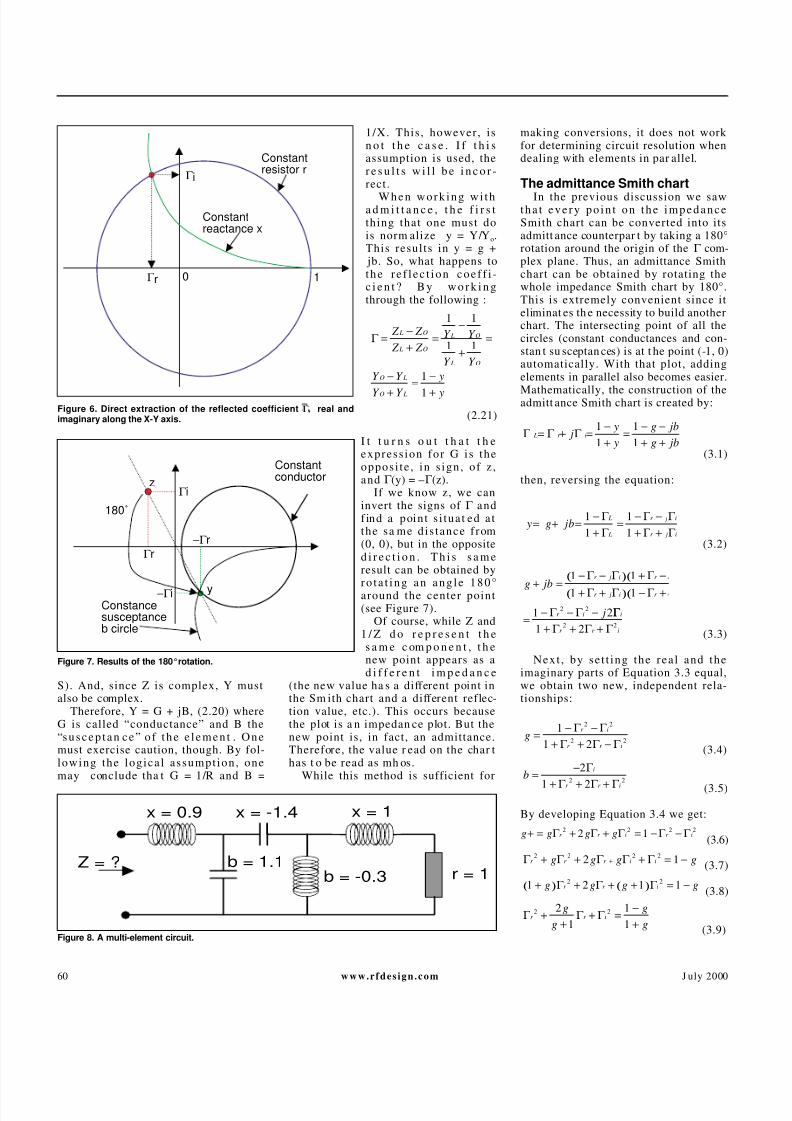
S). And, since Z is complex, Y mustalso be complex.

Therefore, Y = G + jB, (2.20) whereG is called “conductance” and B the“suscep t an ce” o f t he e l emen t . O nemust exercise caution, though. By fol-lowing the logica l assumpt ion , onemay conclude tha t G = 1/R and B =

1/X. This, however, isn o t t h e c a s e . I f t h i sassumption is used, ther e s u l t s w i l l b e i n c o r -rect.

W hen w ork ing w i tha d m i t t a n c e , t h e f i r s tthing that one must dois norm alize y = Y/Yo.This results in y = g +

jb. So, what happens tothe re f l ec t i on coe f f i -c i e n t ? B y w o r k i n gthrough the following :

:

(2.21)

I t t u r n s o u t t h a t t h eexpress ion for G i s theopposi te , in s ign , of z ,and Γ (y) = –Γ (z).

If we know z, we caninvert the signs of Γ andfind a poin t s i tua t ed a tthe sa me d is tance from(0, 0), but in the opposited i r e c t i o n . T h i s s a m eresult can be obtained byro t a t i ng an ang l e 180°around the center point(see Figure 7).

Of course, while Z and1 / Z d o r e p r e s e n t t h es a m e c om p o n e n t , t h enew point appears as ad i f f e r e n t i m p e d a n c e

(the new value ha s a different point inthe Sm ith chart and a different reflec-tion value, etc.). This occurs becausethe plot is a n impedan ce plot. But thenew point is, in fact, an admittance.Therefore, the value r ead on the char thas t o be read as mh os.

While this method is sufficient for

making conversions, it does not work for determining circuit resolution whendealing with elements in par allel.

The admittance Smith chart

In the previous discussion we sawtha t eve ry po in t on t he impedanceSmith chart can be converted into itsadmitt ance counterpar t by taking a 180°rotation around the origin of the Γ com-plex plane. Thus, an admittance Smithchart can be obtained by rotating thewhole impedance Smith chart by 180°.This is extremely convenient since iteliminat es th e necessity to build anotherchart. The intersecting point of all thecircles (constant conductances and con-stan t su sceptan ces) is at t he point (-1, 0)automatically. With that plot, addingelements in parallel also becomes easier.

Mathematically, the construction of theadmitt ance Smith chart is created by:

(3.1)

then, reversing the equation:

(3.2)

(3.3)

Next , by se t t ing the rea l and theimaginary parts of Equation 3.3 equal,we obtain two new, independent rela-tionships:

(3.4)

(3.5)

By developing Equation 3.4 we get:

(3.6)

(3.7)

(3.8)

(3.9)

Γ Γ Γ r r ig

g

g

g

2 22

1

1

1+

++ =

−+

1 2 1 12 2+( ) + + +( ) = −g g g gr r iΓ Γ Γ

Γ Γ Γ Γ Γ r r r i ig g g g2 2 2 22 1+ + + = −+

g g g gr r i r i+ = + + = − −Γ Γ Γ Γ Γ 2 2 2 22 1

bi

r r i

=−

+ + +

2

1 22 2

Γ

Γ Γ Γ

gr i

r r i

=− −

+ + −1

1 2

2 2

2 2

Γ Γ Γ Γ Γ

g jb

j

r j i r

r j i r

r i

+ =

− −( ) + −(

+ +( ) − +(

=− − −

1 1

1 1

1 22 2

Γ Γ Γ

Γ Γ Γ Γ Γ Γ Γ Γ Γ Γ

i

r r i1 22 2+ + +

y g jbL

L

r j i

r j i

= + =−+

=− −+ +

1

1

1

1

Γ Γ

Γ Γ Γ Γ

Γ Γ Γ L r i jy

y

g jb

g jb= + =

−+

=− −+ +

1

1

1

1

Γ =−+

=−

+=

−

+=

−

+

Z Z

Z Z

Y Y

Y Y

Y Y

Y Y

y

y

L O

L O

L O

L O

O L

O L

1 1

1 1

1

1

z

180˚

y

Γ i

Γ r−Γ r

−Γ iConstancesusceptanceb circle

Constantconductor

Figure 7. Results of the 180°rotation.

Γ i

Γ r 0 1

Constant

resistor r

Constant

reactance x

Figure 6. Direct extraction of the reflected coefficient Γ, real andimaginary along the X-Y axis.

x = 0.9 x = -1.4 x = 1

Z = ? b = 1.1

b = -0.3 r = 1

Figure 8. A multi-element circuit.




(3.10)

(3.11)

(3.12)

Which again is a parametric equa-

t ion of the type (x-a)2

+ (y-b)2

= R2

(Equation 3.12), in the complex plane(Γ r , Γ i), of a circle with its coordi-nates centered at (-g/g+1 , 0) and hav-ing a radius of 1/(1+g). Furthermore,By developing (Equation 3.5), we showthat :

(3.13)

(3.14)

(3.15)

(3.16)

(3.17)

which is again a parametric equationo f t h e t y p e ( x - a ) 2 + (y-b)2 = R 2

(Equation 3.17).

Equivalent impedance resolutionWhen solving problems where ele-

men t s i n se r i e s and i n pa ra l l e l a remixed together, one can use the same

Smith chart and rotate it around anypoint where conversions from z to y ory to z exist.

Let’s consider th e net work of Figure8 (the elements are normalized with Zo

= 50 Ω). The series reactance (x) ispositive for inductance and negativefor capaci tors . The susceptance (b)is posit ive for capa cita nce and nega-t ive for in ductan ce.

The circuit needs to to be simplified(see Figure 9). Start ing at the right

Γ Γ r i

b b+( ) + +

=1

1 122

2

Γ Γ Γ Γ r r i i

b b b

2 2

2 22 1

2 1 10+ + + + + − =

Γ Γ Γ Γ r r i i

b

2 22 12

0+ + + + =

1 222 2+ + + =

−Γ Γ Γ

Γ r r i

i

b

b b b br r i i+ + + = −Γ Γ Γ Γ 2 22 2

Γ Γ r ig

g g+

+

+ =

+( )1

1

1

2

2

2

Γ Γ r ig

g

g

g

g

g g

++

+ =

−+

++( )

=+( )

1

1

1

1

1

1

2

2

2

2 2

Γ Γ Γ r r ig

g

g

g

g

g

g

g

22

2

2

2

2

2

1 1

1

1

1

++

++( )

+

−

+( )

=−

+

Figure 10. The network elements plotted on the Smith chart.

Z = ?

x = 0.9 b = 1.1 x = -1.4 b = -0.3x = 1

r = 1

A

B

C

D

Z

Figure 9. The network of Figure 8 with its elements broken out for analysis.




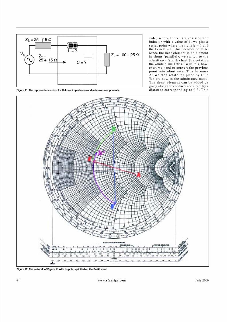
s ide , w here t he re i s a re s i s t o r andinductor with a value of 1, we plot aseries point where the r circle = 1 andthe l circle = 1. This becomes point A.Since the next element is an element

in shunt (paral lel), we switch to theadmittance Smith chart (by rotat ingthe whole plane 180°). To do this, how-ever, we need to convert the previouspoint into admittance. This becomesA’. We then rotat e th e plane by 180°.We are now in the admittance mode.The shunt e lement can be added bygoing along t he conducta nce circle by ad is tan ce corresponding to 0 .3 . This

Figure 12. The network of Figure 11 with its points plotted on the Smith chart.

ZS = 25 - j15 Ω

VS Z* =

25 + j15 Ω

L = ?

C = ?ZL = 100 - j25

Ω

Figure 11. The representative circuit with know impedances and unknown components.




must be done in a counter-clockwisedirection (negative value) and givespoint B. Next, we have another serieselement. We again switch back to theimpedance Smith chart. Before doing

this, it is again necessary to reconvertthe previous point into impedance (itwas an admittance). After the conver-sion, we can deter min e B’. Using th epreviously es tab l i shed rout ine , thechart is again rotat ed 180° to get back to th e impedan ce mode. The serieselement is added by following alongthe resistance circle by a distance cor-responding to 1.4 an d markin g pointC. This has to be done counter-clock-wise (negat ive value). For th e next ele-m e n t , t h e s a m e o p er a t i o n i s p e r -formed(convers ion in to admit tanceand p lane ro ta t ion) . Then move th e

prescribed distance (1.1), in a clock-wise direction (since the value is posi-tive), along the constant conductancecircle. We mark this as D. Finally, wereconvert back to impeda nce modeand add the last element (the seriesi n d u c t o r ) . W e t h e n d e t e r m i n e t h erequired value, z, located at the inter-section of resistor circle 0.2 and reac-tance circle 0.5. Thus z is determinedto be 0.2 +j0.5. If the system charac-terist ic impedan ce is 50 Ω, then Z = 10+ j25 Ω (see Figure 10).

Matching impedances by stepsAnother function of the Smith chart

is the ability to determine impedancematching. This is the reverse opera-tion of finding the equivalent imped-ance of a g iven network . Here , theimpedan ces ar e fixed at the two accessends (often th e source and t he load) asshown in Figure 11. The objective is todesign a network to insert be tweenthem so tha t proper impedance mat ch-ing occurs .

At first glance, it appears that is isno more difficult than finding equiva-len t impedance. But the problem isthat an infini te number of matchingnetwork component combinations can

exist that create similar results. And,other inputs may need to be consid-ered as well (filter type structure, qual-ity factor, limited choice of components,etc.).

The approach chosen to accomplishthis calls for adding series and shuntelements on the Smith chart until thed e s i r e d i m p e d a n c e i s a c h i e v e d .Graphically, i t appears as finding away to l ink the points on the Smithchart.

Again, the best method to illustratethe a pproach is to address th e require-ment as a n example.

The objective is to match a sourceimpedance (ZS) to a load (ZL) a t t he

working frequency of 60 MHz (seeFigure 11). The network stru ctur e hasbeen fixed as a lowpass, L type (anal ternat ive approach i s to v iew theproblem as how to force the load toappea r like an impeda nce of value = ZS

(a complex conjugate of ZS). Here ishow the solution is found.

The first thing to do is to normalizethe different impedance values. If thisis not given, choose a value that is inthe same range as the load/source val-ues. Assume Zo to be 50 Ω. Thus zS =0.5 –j0.3, z*S = 0.5 + j0.3 an d ZL = 2–j0.5.

Next, position th e two points on thechart . Mark A for zL an d D for Z*S.

Then identify the first element con-n e c t e d t o t h e l oa d ( a c a p a c it o r i ns h u n t ) a n d c on v e r t t o a d m i t t a n c e .This gives us point A’.

D e te rmine t he a rc po r t i on w herethe next poin t wi l l appear af ter theconn ection of th e capa citor C. Since wedon’t know the value of C, we don’tknow where to stop. We do, however,k n o w t h e d i r e c t i o n . A C i n s h u n tmeans move in the clock-wise direc-t ion on the admit tance Smith chartun til the value is found . This will bepo in t B (an a dmi t t a nce ). S ince t henext element is a series element, pointB has to be converted to the imped-a n c e p l a n e . P o in t B ’ c a n t h e n b eobtained. Point B’ has to be located ont h e s a m e r e s i s t o r c i r c l e a s D .Graph ically, there is only one solut ionfrom A’ to D, but t he in t erm edia tepoint B (an d hen ce B’) will need t o beveri f ied by a “tes t -and-t r y” se tu p .After having found points B and B’, wecan mea sur e th e lengths of arc A’ – Ban d ar c B’ – D. The first gives the n or-malized susceptance value of C. Thesecond gives the normalized reactancevalue of L. The arc A’ – B measures b

= 0.78 and thus B = 0.78 x Yo = 0.0156mh os. Since ωC = B, th en C = B/ ω =B/(2 π f) = 0.0156/(2 π 60 7) = 41.4 pF.The arc B –- D mea sur es x = 1.2, th usX = 1.2 x Zo = 60 Ω. Since ωL = X,th en L = X/ ω = X/(2 π f) = 60/(2 π607) = 159 nH.

ConclusionGiven today’s wealth of software

and accessibility of high-speed, high-power computers, one may question

the need for such a basic and funda-mental method for determining circuitfundamentals.

In reality, what makes an engineera rea l engineer is not only academ ic

k n o w l e d g e , b u t t h e a b i l i t y t o u s eresources of all types to solve a prob-lem. It is easy to plug a few numbersinto a program a nd have it spit out t hesolutions. And, when the solutions arecomplex and mult ifaceted, having acomputer handy to do the grunt work is “back-savin gly” ha ndy.

However, k nowing u nderlying t heo-ry and principles th at have been port-ed to computer platforms, and wherethey came from, makes th e engineer ordesigner a m ore well rounded an d con-f iden t p ro fess iona l–and makes t heresults more reliable.

About the authorH a r t e r A l p h o n s e i s a C F A E

W ir e l e s s a t M a x i m F r a n ce . H eholds an EE degree from ENS EA inP a r i s , F r a n c e a n d h a s b e e n w i t hMaxim for 7 year s as a F AE special-izing in radio frequency products.E - M a i l : Al p h on se_ H ar t er@com -

puserve.comC h a n K u o - C h a n g i s t h e

Appl ica t ions Manager for MaximF r a n c e . H e h o l d s a n E E d e g r e efrom UCL univers i ty in Louvain ,Belgum. H e joined Maxim 8 m onthsago and was previously employedby Xemics, Switzerla nd, workingf o r t h e i r T r a n s c e i v e r P r o d u c tMarketing. E-Mail: Ma x_Kcc@com -

puserve.com .

smith chart fundamentals

Documents