smart motion sensor for navigated prosthetic surgery
TRANSCRIPT

HAL Id: pastel-00691192https://pastel.archives-ouvertes.fr/pastel-00691192
Submitted on 25 Apr 2012
HAL is a multi-disciplinary open accessarchive for the deposit and dissemination of sci-entific research documents, whether they are pub-lished or not. The documents may come fromteaching and research institutions in France orabroad, or from public or private research centers.
L’archive ouverte pluridisciplinaire HAL, estdestinée au dépôt et à la diffusion de documentsscientifiques de niveau recherche, publiés ou non,émanant des établissements d’enseignement et derecherche français ou étrangers, des laboratoirespublics ou privés.
Smart motion sensor for navigated prosthetic surgeryGöntje Caroline Claasen
To cite this version:Göntje Caroline Claasen. Smart motion sensor for navigated prosthetic surgery. Other. Ecole Na-tionale Supérieure des Mines de Paris, 2012. English. �NNT : 2012ENMP0008�. �pastel-00691192�

T
H
È
S
E
INSTITUT DES SCIENCES ET TECHNOLOGIES
École doctorale nO432: Sciences des Métiers de l’Ingénieur (SMI)
Doctorat ParisTech
T H È S Epour obtenir le grade de docteur délivré par
l’École Nationale Supérieure des Mines de Paris
Spécialité “Mathématique et Automatique”
présentée et soutenue publiquement par
Göntje Caroline CLAASENle 17 février 2012
Capteur de mouvement intelligentpour la chirurgie prothétique naviguée
Directeur de thèse: Philippe MARTIN
JuryMme Isabelle FANTONI-COICHOT, Chargée de recherche HDR, Rapporteur
Heudiasyc UMR CNRS 6599, Université de Technologie de CompiègneM. Philippe POIGNET, Professeur, LIRMM UM2-CNRS RapporteurM. Tarek HAMEL, Professeur, I3S UNSA-CNRS ExaminateurM. Wilfrid PERRUQUETTI, Professeur, LAGIS FRE CNRS 3303-UL1-ECL ExaminateurM. Frédéric PICARD, Docteur en médecine, chirurgien orthopédiste, Examinateur
Golden Jubilee National Hospital, GlasgowM. Philippe MARTIN, Maître de recherche, Centre Automatique et Systèmes, Examinateur
MINES ParisTechMINES ParisTech
Centre Automatique et Systèmes (CAS)60, Bd Saint Michel - 75006 Paris - France


T
H
È
S
E
INSTITUT DES SCIENCES ET TECHNOLOGIES
Graduate School nO432: Sciences des Métiers de l’Ingénieur (SMI)
ParisTech
P H D T H E S I STo obtain the Doctor’s degree from
École Nationale Supérieure des Mines de Paris
Speciality “Mathématique et Automatique”
defended in public by
Göntje Caroline CLAASENon February 17, 2012
Smart motion sensorfor navigated prosthetic surgery
Thesis advisor: Philippe MARTIN
CommitteeMs. Isabelle FANTONI-COICHOT, Chargée de recherche HDR, Reviewer
Heudiasyc UMR CNRS 6599, Université de Technologie de CompiègneMr. Philippe POIGNET, Professor, LIRMM UM2-CNRS ReviewerMr. Tarek HAMEL, Professor, I3S UNSA-CNRS ExaminerMr. Wilfrid PERRUQUETTI, Professor, LAGIS FRE CNRS 3303-UL1-ECL ExaminerMr. Frédéric PICARD, MD, Orthpaedic Surgeon, Golden Jubilee National Hospital, Glasgow ExaminerMr. Philippe MARTIN, Maître de recherche, Centre Automatique et Systèmes, Examiner
MINES ParisTechMINES ParisTech
Centre Automatique et Systèmes (CAS)60, Bd Saint Michel - 75006 Paris - France

Göntje Caroline CLAASEN
Centre Automatique et SystèmesUnité Mathématiques et SystèmesMINES ParisTech60 boulevard St Michel75272 Paris CedexFrance.
E-mail: [email protected], [email protected]
Key words. - optical-inertial data fusion, Kalman filtering, nonlinear observers,computer-assisted surgery, servo-controlled handheld toolMots clés. - fusion de données optiques-inertielles, filtrage de Kalman, observateursnon-linéaires, chirurgie assistée par ordinateur, outil à main asservi

Education is the most powerful weapon which you can use to change the world.
Nelson Mandela


Remerciements
Tout d’abord je tiens à remercier Philippe Martin pour avoir encadré cette thèsependant trois ans. Merci de votre enthousiasme pour ce projet, pour la recherche engénérale et pour les choses qui marchent. Merci pour votre soutien et vos conseils.
Je souhaite remercier Isabelle Fantoni-Coichot ainsi que Philippe Poignet qui ontaccepté d’être les rapporteurs de cette thèse. Je remercie également Tarek Hamel, WilfridPerruquetti et Frédéric Picard qui m’ont fait l’honneur de participer au jury de soutenance.
Un grand merci à tous les membres du Centre Automatique et Systèmes pour leursoutien et leurs conseils et pour avoir répondu à mes nombreuses questions sur la Franceet la langue française. Merci à mes camarades de thèse Eric, Florent et Pierre-Jean. Merciégalement à Erwan pour son aide.
I would like to thank Frédéric Picard and Angela Deakin from the Golden JubileeHospital in Glasgow for having introduced me to the world of orthopaedic surgery.
Danke meiner Familie, besonders meinen Eltern und Großeltern, der Familie Bezansonund natürlich Gregor für ihre immerwährende Unterstützung, die dieses Abenteuer erstmöglich gemacht hat.
Je remercie le Fonds AXA pour la Recherche pour le financement de cette thèse.


Smart motion sensorfor navigated prosthetic surgery


Résumé
Nous présentons un système de tracking optique-inertiel qui consiste en deux camérasstationnaires et une Sensor Unit avec des marqueurs optiques et une centrale inertielle. LaSensor Unit est fixée sur l’objet suivi et sa position et son orientation sont déterminées parun algorithme de fusion de données. Le système de tracking est destiné à asservir un outilà main dans un système de chirurgie naviguée ou assistée par ordinateur. L’algorithmede fusion de données intègre les données des différents capteurs, c’est-à-dire les donnéesoptiques des caméras et les données inertielles des accéléromètres et gyroscopes. Nousprésentons différents algorithmes qui rendent possible un tracking à grande bande passanteavec au moins 200Hz avec des temps de latence bas grâce à une approche directe et desfiltres dits invariants qui prennent en compte les symétries du système. Grâce à cespropriétés, le système de tracking satisfait les conditions pour l’application désirée. Lesystème a été implémenté et testé avec succès avec un dispositif expérimental.
Abstract
We present an optical-inertial tracking system which consists of two stationary camerasand a Sensor Unit with optical markers and an inertial measurement unit (IMU). ThisSensor Unit is attached to the object being tracked and its position and orientation aredetermined by a data fusion algorithm. The tracking system is to be used for servo-controlling a handheld tool in a navigated or computer-assisted surgery system. Thedata fusion algorithm integrates data from the different sensors, that is optical data fromthe cameras and inertial data from accelerometers and gyroscopes. We present differentalgorithms which ensure high-bandwidth tracking with at least 200Hz with low latenciesby using a direct approach and so-called invariant filters which take into account systemsymmetries. Through these features, the tracking system meets the requirements for beingused in the desired application. The system was successfully implemented and tested withan experimental setup.
xi


Contents
1 Introduction 11.1 Navigated Surgery Systems . . . . . . . . . . . . . . . . . . . . . . . . . . . . . 21.2 Handheld Tools for Navigated Surgery . . . . . . . . . . . . . . . . . . . . . . 51.3 Smart Handheld Tool . . . . . . . . . . . . . . . . . . . . . . . . . . . . . . . . 61.4 Tracking for the Smart Handheld Tool . . . . . . . . . . . . . . . . . . . . . . 71.5 Servo-Control for 1D model . . . . . . . . . . . . . . . . . . . . . . . . . . . . 91.6 Outline . . . . . . . . . . . . . . . . . . . . . . . . . . . . . . . . . . . . . . . . . 141.7 Publications . . . . . . . . . . . . . . . . . . . . . . . . . . . . . . . . . . . . . . 15
2 Optical-Inertial Tracking System 172.1 System Setup . . . . . . . . . . . . . . . . . . . . . . . . . . . . . . . . . . . . . 17
2.1.1 Optical System . . . . . . . . . . . . . . . . . . . . . . . . . . . . . . . . 172.1.2 Inertial Sensors . . . . . . . . . . . . . . . . . . . . . . . . . . . . . . . 22
2.2 Mathematical Model . . . . . . . . . . . . . . . . . . . . . . . . . . . . . . . . . 242.2.1 Coordinate systems . . . . . . . . . . . . . . . . . . . . . . . . . . . . . 242.2.2 Quaternions . . . . . . . . . . . . . . . . . . . . . . . . . . . . . . . . . 242.2.3 Dynamics Model . . . . . . . . . . . . . . . . . . . . . . . . . . . . . . . 272.2.4 Output Model . . . . . . . . . . . . . . . . . . . . . . . . . . . . . . . . 272.2.5 Noise Models . . . . . . . . . . . . . . . . . . . . . . . . . . . . . . . . . 282.2.6 Complete Model . . . . . . . . . . . . . . . . . . . . . . . . . . . . . . . 31
3 State of the Art 333.1 Computer Vision and Optical Tracking . . . . . . . . . . . . . . . . . . . . . . 33
3.1.1 Monocular Tracking . . . . . . . . . . . . . . . . . . . . . . . . . . . . . 343.1.2 Stereo Tracking . . . . . . . . . . . . . . . . . . . . . . . . . . . . . . . 373.1.3 Problems/Disadvantages . . . . . . . . . . . . . . . . . . . . . . . . . . 50
3.2 Optical-Inertial Tracking Systems . . . . . . . . . . . . . . . . . . . . . . . . . 503.2.1 Systems Presented in the Literature . . . . . . . . . . . . . . . . . . . 503.2.2 Motivation of Our Approach . . . . . . . . . . . . . . . . . . . . . . . 53
3.3 Calibration . . . . . . . . . . . . . . . . . . . . . . . . . . . . . . . . . . . . . . 54
xiii
CONTENTS
3.3.1 Camera Calibration . . . . . . . . . . . . . . . . . . . . . . . . . . . . . 543.3.2 IMU Calibration . . . . . . . . . . . . . . . . . . . . . . . . . . . . . . . 553.3.3 Optical-Inertial Calibration . . . . . . . . . . . . . . . . . . . . . . . . 57
4 Data Fusion 594.1 Motivation . . . . . . . . . . . . . . . . . . . . . . . . . . . . . . . . . . . . . . . 594.2 Extended Kalman Filter . . . . . . . . . . . . . . . . . . . . . . . . . . . . . . 61
4.2.1 Continuous EKF . . . . . . . . . . . . . . . . . . . . . . . . . . . . . . . 614.2.2 Multiplicative EKF (MEKF) . . . . . . . . . . . . . . . . . . . . . . . 624.2.3 Continuous-Discrete EKF . . . . . . . . . . . . . . . . . . . . . . . . . 63
4.3 Data Fusion for Optical-Inertial Tracking . . . . . . . . . . . . . . . . . . . . 644.3.1 System Observability . . . . . . . . . . . . . . . . . . . . . . . . . . . . 644.3.2 Direct and Indirect Approaches . . . . . . . . . . . . . . . . . . . . . . 654.3.3 MEKF . . . . . . . . . . . . . . . . . . . . . . . . . . . . . . . . . . . . . 654.3.4 Right- and Left-Invariant EKF . . . . . . . . . . . . . . . . . . . . . . 674.3.5 Covariance Parameters . . . . . . . . . . . . . . . . . . . . . . . . . . . 774.3.6 Continuous-Discrete and Multi-rate . . . . . . . . . . . . . . . . . . . 77
4.4 RIEKF for Calibration . . . . . . . . . . . . . . . . . . . . . . . . . . . . . . . 794.4.1 Influence of calibration errors on the RIEKF . . . . . . . . . . . . . . 804.4.2 Calibration of Marker-Body Rotation with RIEKF . . . . . . . . . . 87
5 Implementation and Experimental Results 895.1 Experimental Setup . . . . . . . . . . . . . . . . . . . . . . . . . . . . . . . . . 89
5.1.1 Cameras and Optical Markers . . . . . . . . . . . . . . . . . . . . . . . 895.1.2 Inertial Sensors . . . . . . . . . . . . . . . . . . . . . . . . . . . . . . . 945.1.3 Sensor Unit . . . . . . . . . . . . . . . . . . . . . . . . . . . . . . . . . . 945.1.4 Data Acquisition . . . . . . . . . . . . . . . . . . . . . . . . . . . . . . . 945.1.5 Algorithm Implementation . . . . . . . . . . . . . . . . . . . . . . . . . 975.1.6 Tracking References . . . . . . . . . . . . . . . . . . . . . . . . . . . . . 103
5.2 Experiments . . . . . . . . . . . . . . . . . . . . . . . . . . . . . . . . . . . . . . 1065.2.1 Experiment 1: static case . . . . . . . . . . . . . . . . . . . . . . . . . 1065.2.2 Experiment 2: slow linear motion . . . . . . . . . . . . . . . . . . . . 1065.2.3 Experiment 3: fast oscillating linear motion . . . . . . . . . . . . . . 1065.2.4 Experiment 4: static orientations . . . . . . . . . . . . . . . . . . . . . 106
5.3 Results . . . . . . . . . . . . . . . . . . . . . . . . . . . . . . . . . . . . . . . . . 1105.3.1 General Observations . . . . . . . . . . . . . . . . . . . . . . . . . . . . 1105.3.2 Precision and Accuracy . . . . . . . . . . . . . . . . . . . . . . . . . . . 1185.3.3 High-Bandwidth Tracking . . . . . . . . . . . . . . . . . . . . . . . . . 1195.3.4 Influence of Sensor Unit Calibration . . . . . . . . . . . . . . . . . . . 124
5.4 Calibration . . . . . . . . . . . . . . . . . . . . . . . . . . . . . . . . . . . . . . 128
xiv

CONTENTS
5.4.1 Optical System . . . . . . . . . . . . . . . . . . . . . . . . . . . . . . . . 1285.4.2 Accelerometers . . . . . . . . . . . . . . . . . . . . . . . . . . . . . . . . 1295.4.3 Gyroscopes . . . . . . . . . . . . . . . . . . . . . . . . . . . . . . . . . . 1305.4.4 Sensor Unit . . . . . . . . . . . . . . . . . . . . . . . . . . . . . . . . . . 130
6 Conclusion 135
xv


Chapter 1
Introduction
Les systèmes de chirurgie assistée par ordinateur sont de plus en plus utilisés dans les sallesopératoires. Pour la pose de prothèses de genou, par exemple, un tel système mesure despoints anatomiques, calcule la position optimale de la prothèse et indique les lignes decoupe. Actuellement, les coupes sont exécutées à l’aide de guides de coupe mécaniques,mais une technique de coupe sans guide mécanique est demandée par les chirurgiens.Différentes méthodes ont été proposées, par exemple utilisant un feedback visuel pour lechirurgien ou des systèmes robotiques. Nous considérons un outil à main asservi qui utiliseun système de tracking pour déterminer la position de l’outil par rapport au patient et auxplans de coupe désirés. Le tracking doit avoir une bande passante d’au moins 200Hz pourpouvoir suivre le mouvement rapide de l’outil.
Comme aucun système adapté aux conditions de la salle opératoire et au coût possibled’un système de chirurgie n’existe, nous proposons un nouveau système de tracking quiutilise des capteurs optiques et inertiels pour déterminer la position et l’orientation d’unoutil à main asservi.
Le système a une grande bande passante grâce aux capteurs inertiels haute fréquence.Il a un temps de latence réduit par rapport à des systèmes similaires grâce à deuxcaractéristiques: nous proposons une approche directe utilisant les données brutes descapteurs sans faire des calculs complexes comme dans l’approche standard, et nousutilisons des algorithmes de fusion de données qui prennent en compte les symmétriesdu système ce qui réduit le temps de calcul.
Nous présentons des résultats de simulation pour un modèle simple d’un outil à mainasservi avec différents systèmes de tracking illustrant l’intérêt d’un tel systéme.
1

Chapter 1. Introduction
1.1 Navigated Surgery Systems
Computer-assisted or navigated surgery systems have become more and more common inoperating rooms over the last 15 years [DiGioia et al., 2004].
In orthopedic surgery systems, e.g. for knee replacement, it is important to makeaccurate bone cuts and place the prosthesis correctly. The system acquires relevantpatient anatomical landmarks and calculates appropriate prosthesis placement basedon built up frame of reference. It then defines the desired cutting planes for theknee prosthesis [DiGioia et al., 2004]. Such a computer-assisted surgery system for kneereplacement is described in detail in [Stulberg et al., 2004].
Here we consider so-called image-free or CT-free surgery systems. Image-guidedsystems [Jolesz et al., 1996] use image data from video, computer tomography (CT),magnetic-resonance imaging (MRI) or ultrasound (US) to obtain patient anatomicalinformation before and during surgery. These imaging techniques demand for importantprocessing and some, like CT scans, also expose the patient to radiation. In contrastto this, image-free systems use optical tracking to determine anatomical landmarks[Mösges and Lavallé, 1996, DiGioia et al., 2004]. They make use of cameras but unlikeimage-based systems they do not treat the whole image. Instead, the cameras observeoptical markers which are attached to the patient’s bones. The optical markers aredetected in the images and only the information of their point coordinates are usedin the subsequent analysis instead of the whole image. The first image-free systemfor knee replacement used in an operating room was presented in [Leitner et al., 1997].This system was later commercialized as OrthoPilot (Aesculap AG, Tuttlingen, Germany[Aesculap AG, 2011]). Figure 1.1 shows the OrthoPilot.
It is important to note the difference between computer-assisted surgery systems androbotic surgery systems. In the latter, surgical procedures are executed autonomouslyby a robotic system [Taylor and Stoianovici, 2003]. Robotic systems can perform theseprocedures with high accuracy but rise questions about safety and liability [Davies, 1996].Computer-assisted surgery systems on the other hand, let the surgeon keep the controlover the whole surgical procedure.
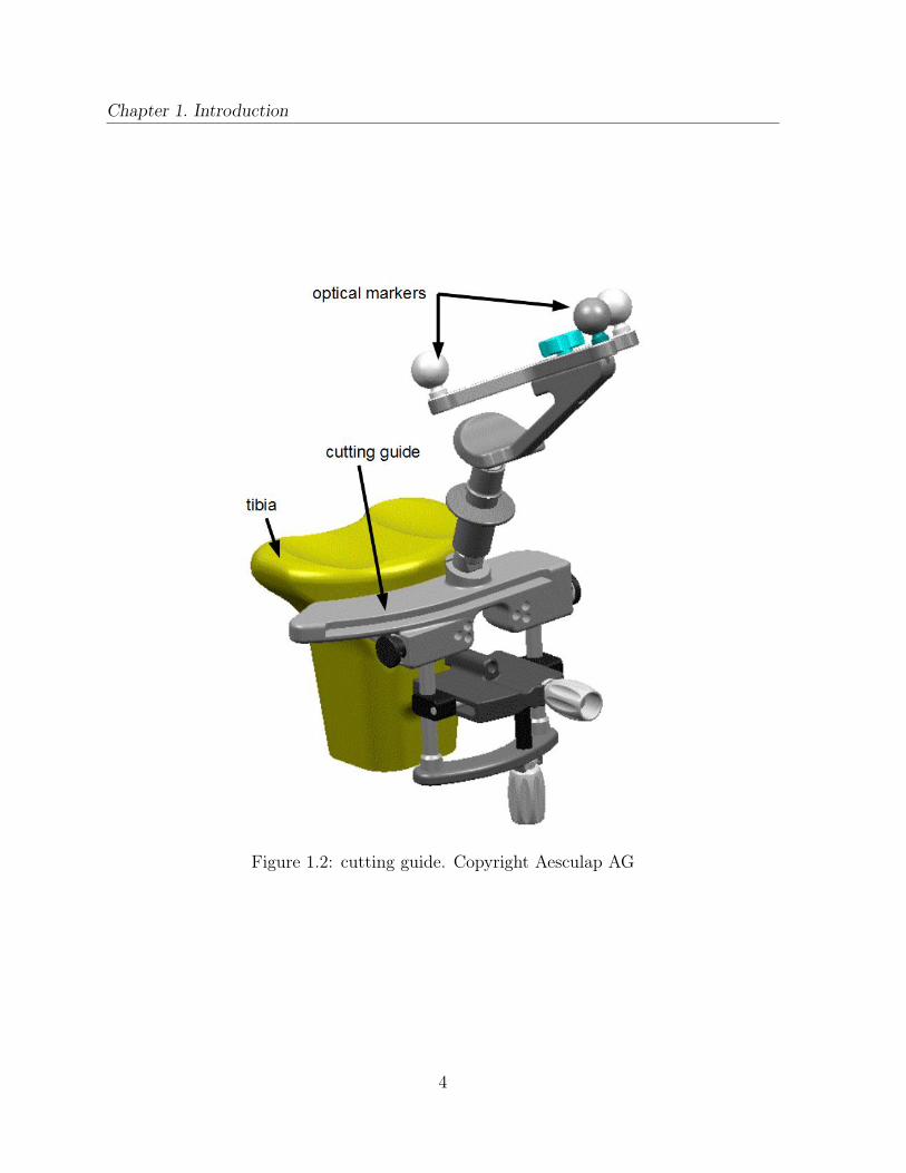
We now return to the original problem of cutting bones for knee replacement. Incurrent systems, the bone cuts are executed with the help of cutting guides (also calledcutting jigs) which are fixed to the patient’s bone in accordance with the desired cuttingplanes [Stulberg et al., 2004]. They guide the bone saw mechanically with good accuracy.A cutting guide is depicted in Figure 1.2. Cutting guides have two main drawbacks:Mounting and repositioning the guide takes time and the procedure is invasive becausethe guide is pinned to the bone with screws.
2

1.1. NAVIGATED SURGERY SYSTEMS
Figure 1.1: OrthoPilot® orthopaedic navigation system for knee replacement. CopyrightAesculap AG
3
Chapter 1. Introduction
Figure 1.2: cutting guide. Copyright Aesculap AG
4

1.2. HANDHELD TOOLS FOR NAVIGATED SURGERY
1.2 Handheld Tools for Navigated Surgery
Using a handheld saw without any cutting guides would have several advantages: theprocedure would be less invasive, demand less surgical material and save time. Obviously,it would have to produce cuts with the same or even better accuracy to be a valuableimprovement.
While a robotic system could achieve this task of cutting along a desired path, manysurgeons wish to keep control over the cutting procedure. Therefore, an intelligenthandheld tool should be used which combines the surgeon’s skills with the accuracy,precision and speed of a computer-controlled system. Such a tool should be small andlightweight so as not to impede on the surgeon’s work, compatible with existing computer-assisted surgery systems and relatively low-cost.
Controlling the tool position and keeping it along the desired cutting path necessitatethe following steps:
1. define desired cutting plane relative to the patient,
2. track tool position and orientation relative to the patient and
3. compare desired and actual positions and correct the tool position accordingly.
The first step is done by the surgery system and the second by a tracking system. Step 3can be executed either by the surgeon, by a robotic arm or directly by the handheld tool.
Several handheld tools have been developed in recent years, employing differentstrategies for the control of the tool position. In [Haider et al., 2007], the patient’s boneand a handheld saw are tracked by an optical tracking system and the actual and desiredcutting planes are shown on a screen. The surgeon corrects the position of the sawbased on what he sees on the screen to make the actual and desired planes coincide.This approach is called "navigated freehand cutting" by the authors. A robotic armis used in [Knappe et al., 2003] to maintain the tool orientation and correct deviationscaused by slipping or inhomogeneous bone structure. The arm is tracked by an opticaltracking system and internal encoders. The optical tracking also follows the patient’sposition. In [Maillet et al., 2005], a cutting guide is held by a robotic arm at the desiredposition, thus eliminating the problems linked to attaching cutting guides to the bone andrepositioning. Several commercial systems with robotic arms are available, for examplethe Mako Rio (Mako Surgical, Fort Lauderdale, USA [Mako Surgical Corp., 2011]) andthe Acrobot Sculptor (Acrobot LTD) [Jakopec et al., 2003].
Several "intelligent" handheld tools which are able to correct deviations from thedesired cutting plane automatically by adapting the blade/drill position without arobotic arm have been developed. The systems presented in [Brisson et al., 2004]and [Kane et al., 2009] use an optical tracking system. [Schwarz et al., 2009] uses an
5

Chapter 1. Introduction
optical tracking system to determine the position of the patient and of the tool which alsocontains inertial sensors. The authors estimated the necessary tracking frequency to beof 100Hz to be able to compensate the surgeon’s hand tremor which range is up to 12 Hzand the patient’s respiratory motion.
The systems presented so far determine a desired cutting path based on absoluteposition measurements of tools and patients. In contrast, tools have been developedwhich are controlled relative to the patient only. [Ang et al., 2004] presents a handheldtool which uses accelerometers and magnetometers for tremor compensation. A handheldtool with actuators controlling the blade position is presented in [Follmann et al., 2010].The goal is to cut the skull only up to a certain depth while the surgeon guides the toolalong a path. While an optical tracking system is used in this work, an alternative versionwith a tracking system using optical and inertial sensors is presented in [Korff et al., 2010].
Three different approaches to bone cutting without cutting guides have been comparedin [Cartiaux et al., 2010]: freehand, navigated freehand (surgeon gets visual feedbackprovided by a navigation system; similar to [Haider et al., 2007]) and with an industrialrobot. The authors find that the industrial robot gives the best result and freehandcutting the worst.
The authors of [Haider et al., 2007] compared their navigated freehand cuts to thosewith conventional cutting jigs and found the cuts had rougher surfaces but betteralignment.
1.3 Smart Handheld Tool
The handheld tool we consider here is supposed to be an extension for an image-freeor image-based computer-assisted surgery system, hence it can make use of an opticaltracking system but not of an active robotic arm. The tool is to be servo-controlled withmotors in the tool joints which can change the blade position. We use a saw as an examplebut the same applies to drilling, pinning or burring tools. In the case of a saw for kneereplacement surgery, the new smart handheld tool would eliminate the need for cuttingguides.
The tracking system and particularly its bandwidth are a key for good performance ofthe servo-control. Firstly, the tracking system should be able to follow human motion andespecially fast movements - these could be due to a sudden change of bone structure whilecutting or to slipping of the surgeon’s hand. These are the movements to be corrected.Secondly, it should be fast enough to let the servo-control make the necessary corrections.The faster the correction, the smaller the deviation will be. Finally, the servo-controlshould make the correction before the surgeon notices the error to avoid conflict betweenthe control and the surgeon’s reaction. We estimate the surgeon’s perception time to be
6
1.4. TRACKING FOR THE SMART HANDHELD TOOL
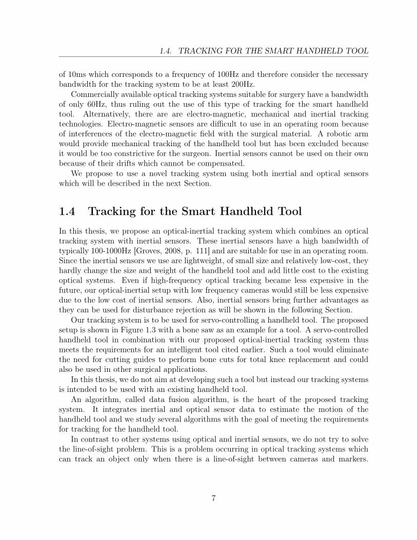
of 10ms which corresponds to a frequency of 100Hz and therefore consider the necessarybandwidth for the tracking system to be at least 200Hz.
Commercially available optical tracking systems suitable for surgery have a bandwidthof only 60Hz, thus ruling out the use of this type of tracking for the smart handheldtool. Alternatively, there are are electro-magnetic, mechanical and inertial trackingtechnologies. Electro-magnetic sensors are difficult to use in an operating room becauseof interferences of the electro-magnetic field with the surgical material. A robotic armwould provide mechanical tracking of the handheld tool but has been excluded becauseit would be too constrictive for the surgeon. Inertial sensors cannot be used on their ownbecause of their drifts which cannot be compensated.
We propose to use a novel tracking system using both inertial and optical sensorswhich will be described in the next Section.
1.4 Tracking for the Smart Handheld Tool
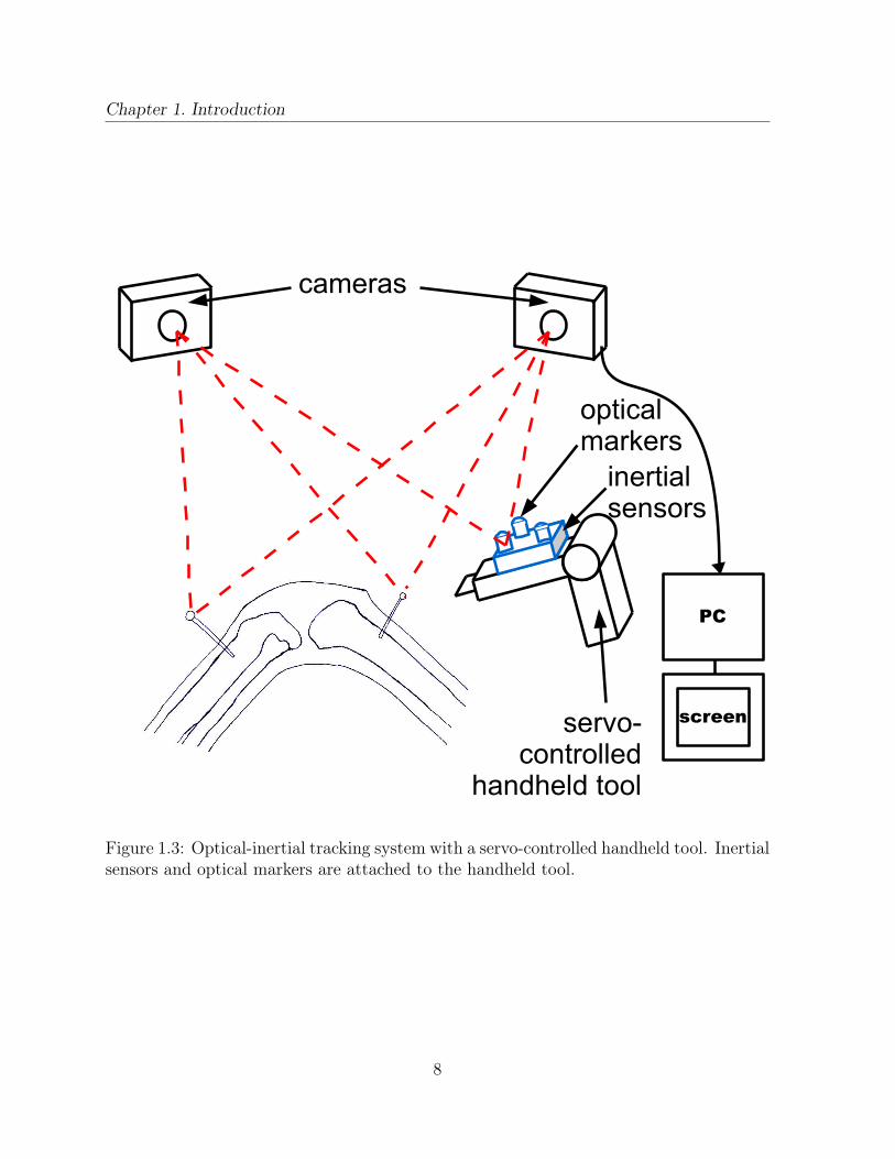
In this thesis, we propose an optical-inertial tracking system which combines an opticaltracking system with inertial sensors. These inertial sensors have a high bandwidth oftypically 100-1000Hz [Groves, 2008, p. 111] and are suitable for use in an operating room.Since the inertial sensors we use are lightweight, of small size and relatively low-cost, theyhardly change the size and weight of the handheld tool and add little cost to the existingoptical systems. Even if high-frequency optical tracking became less expensive in thefuture, our optical-inertial setup with low frequency cameras would still be less expensivedue to the low cost of inertial sensors. Also, inertial sensors bring further advantages asthey can be used for disturbance rejection as will be shown in the following Section.
Our tracking system is to be used for servo-controlling a handheld tool. The proposedsetup is shown in Figure 1.3 with a bone saw as an example for a tool. A servo-controlledhandheld tool in combination with our proposed optical-inertial tracking system thusmeets the requirements for an intelligent tool cited earlier. Such a tool would eliminatethe need for cutting guides to perform bone cuts for total knee replacement and couldalso be used in other surgical applications.
In this thesis, we do not aim at developing such a tool but instead our tracking systemsis intended to be used with an existing handheld tool.
An algorithm, called data fusion algorithm, is the heart of the proposed trackingsystem. It integrates inertial and optical sensor data to estimate the motion of thehandheld tool and we study several algorithms with the goal of meeting the requirementsfor tracking for the handheld tool.
In contrast to other systems using optical and inertial sensors, we do not try to solvethe line-of-sight problem. This is a problem occurring in optical tracking systems whichcan track an object only when there is a line-of-sight between cameras and markers.
7
Chapter 1. Introduction
cameras
PC
screen
optical markers
servo-controlled
handheld tool
inertial sensors
Figure 1.3: Optical-inertial tracking system with a servo-controlled handheld tool. Inertialsensors and optical markers are attached to the handheld tool.
8

1.5. SERVO-CONTROL FOR 1D MODEL
In some optical-inertial systems presented in the literature, tracking depends on theinertial sensors only when there is no line-of-sight. Our goal is a tracking system witha high bandwidth and low latency, i.e. the tracking values should be available with aslittle delay as possible after a measurement has been made. This requires an algorithmwhich is particularly adapted to this problem and which reduces latency compared tosimilar systems using optical and inertial sensors as presented in [Tobergte et al., 2009]or [Hartmann et al., 2010] for example. High-bandwidth tracking is achieved by usinginertial sensors with a sample rate of at least 200Hz and by executing the data fusionalgorithm at this rate. To make tracking with low latencies possible, we propose analgorithm with a direct approach, i.e. it uses sensor data directly as inputs. Thisis opposed to the standard indirect approach which demands for computations on themeasured values before using them in the data fusion algorithm. To further reduce latency,our algorithm takes into account the system geometry which should reduce computationalcomplexity.
The following Section shows the positive effect of high-bandwidth optical-inertialtracking on servo-control of a handheld tool by means of a simulation with a simplemodel. In the rest of the thesis, we will concentrate on the setup of the optical-inertialtracking system and on the data fusion algorithm which integrates optical and inertialsensor data. We will discuss calibration of the hybrid setup and present an experimentalsetup and experimental results which show that the optical-inertial tracking system cantrack fast human motion. While we do not implement the servo-control we develop thenecessary components for a high-bandwidth low-latency tracking system suitable to beused to servo-control a handheld tool in a computer-assisted surgery system.
1.5 Servo-Control for 1D model
In this Section, we are going to show the effect of a higher bandwidth in a Mat-lab/Simulink [Mathworks, 2011] simulation using a simple model of a handheld bone-cutting tool which is servo-controlled using different kind of measurements.
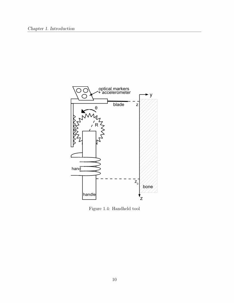
The tool in Figure 1.4 consists of a handle and a blade connected by a gearingmechanism which is actuated by a motor. The goal is to cut in y direction at a desiredheight zr. The surgeon moves the tool in y direction at a speed v. A deviation fromthe desired zr due to a change of bone structure is modeled by a disturbance D actingalong z. In this simple model we assume that the disturbances can make the tool movein z direction only, which means that the tool’s motion is constrained along z except forthe cutting motion along y.
9
Chapter 1. Introduction
z
y
z
z0
R
θ
handle
bone
blade
optical markers
hand
+ accelerometer
Figure 1.4: Handheld tool
10

1.5. SERVO-CONTROL FOR 1D MODEL
The blade position z is determined by
z = Rθ + z0 (1.1)and mz = F +D +mg (1.2)
where R is the radius of the gear wheel, θ the wheel’s angular position, z0 the handleposition, F the force applied by the gear, m the mass of the subsystem carrying the bladeand g is gravity. The motor is governed by
Jθ = U −RF
where J is the motor and gear inertia and U the control input. Combining these equationsgives
z = U
mR + J/R´¹¹¹¹¹¹¹¹¹¹¹¹¹¹¹¹¹¹¹¹¹¹¸¹¹¹¹¹¹¹¹¹¹¹¹¹¹¹¹¹¹¹¹¹¹
u
+ D
m + J/R2+ z0 − g
1 +mR2/J´¹¹¹¹¹¹¹¹¹¹¹¹¹¹¹¹¹¹¹¹¹¹¹¹¹¹¹¹¹¹¹¹¹¹¹¹¹¹¹¹¹¹¹¹¹¹¹¹¹¹¹¹¹¹¹¹¹¹¹¹¹¹¹¹¹¹¹¹¹¹¹¸¹¹¹¹¹¹¹¹¹¹¹¹¹¹¹¹¹¹¹¹¹¹¹¹¹¹¹¹¹¹¹¹¹¹¹¹¹¹¹¹¹¹¹¹¹¹¹¹¹¹¹¹¹¹¹¹¹¹¹¹¹¹¹¹¹¹¹¹¹¹¹
d
+g . (1.3)
This yields the simplified system
z = v (1.4)v = u + d + g . (1.5)
The variable d includes the disturbance D due to bone structure as well as disturbancesdue to the surgeon motion (modeled by z0).
An optical tracking system measures the position zm = z with a frequency of1/T = 50Hz at discrete instants zm,k = zm(kT ), an inertial sensor (accelerometer) measuresam = u + d + ab where ab is the accelerometer constant bias.
The inertial measurements are considered continuous because their frequency is muchhigher than that of the optical ones.
We now present three systems using different types of measurements in a standardservo-control design. In all three cases, we do not take measurement noise into accountand l, L, L, h and K are appropriately calculated constant gains. The disturbance d ismodeled as a constant:
d = 0 .
System 1 uses only optical measurements zm,k. An observer estimates the statex = [z, v, d + g]T :
prediction: ˙x− =⎡⎢⎢⎢⎢⎢⎣
v−
u + (d + g)−
0
⎤⎥⎥⎥⎥⎥⎦=⎡⎢⎢⎢⎢⎢⎣
0 1 00 0 10 0 0
⎤⎥⎥⎥⎥⎥⎦x− +
⎡⎢⎢⎢⎢⎢⎣
010
⎤⎥⎥⎥⎥⎥⎦u (1.6)
correction: xk = x−k +L(zm,k−1 − zk−1) (1.7)
11

Chapter 1. Introduction
where x−k = ∫kT
kT−T˙x−(τ)dτ with x−(kT − T ) = xk−1. The state estimation is used in the
controller which readsuk = −Kxk + hzr .
This system corresponds to the case where only an optical tracking system is used.System 2 uses both optical and inertial data and represents the setup we propose in
Chapter 2. A first observer with state x = [z, v, ab − g]T , measured input am and discreteoptical measurements zm,k reads:
prediction: ˙x− =⎡⎢⎢⎢⎢⎢⎣
v
am − (ab − g)−
0
⎤⎥⎥⎥⎥⎥⎦=⎡⎢⎢⎢⎢⎢⎣
0 1 00 0 −10 0 0
⎤⎥⎥⎥⎥⎥⎦x− +
⎡⎢⎢⎢⎢⎢⎣
010
⎤⎥⎥⎥⎥⎥⎦am (1.8)
correction: xk = x−k +L(zm,k−1 − zk−1) (1.9)
where x−k = ∫kT
kT−T˙x−(τ)dτ with x−(kT − T ) = xk−1. This observer gives a continuous
estimation z(t) which is used as a measurement zm(t) for a second observer with statex = [z, v, d + g]T :
˙x =
⎡⎢⎢⎢⎢⎢⎢⎣
ˆv(g + ˜ )d + u
0
⎤⎥⎥⎥⎥⎥⎥⎦
+ L(zm − ˆz) =⎡⎢⎢⎢⎢⎢⎣
0 1 00 0 10 0 0
⎤⎥⎥⎥⎥⎥⎦
ˆx +⎡⎢⎢⎢⎢⎢⎣
010
⎤⎥⎥⎥⎥⎥⎦u + L(zm − ˆz) (1.10)
This continuous state estimation of the second observer is used in the controller whichreads
u = −K ˆx + hzr .
In system 3 which uses optical and inertial data we suppose that tracking and controlare more tightly coupled than in system 2. A first observer is used to estimate thedisturbance d with inertial measurements am = u + d + ab:
˙d + ab = l(am − u − (d + ab)) (1.11)
This observer gives a continuous estimation d + ab(t) which is used as input for the secondcontroller-observer. Its state is x = [z, v, ab−g]T and it uses discrete optical measurementszm,k:
prediction: ˙x− =⎡⎢⎢⎢⎢⎢⎣
v−
u + (d+ab) − (ab−g)−0
⎤⎥⎥⎥⎥⎥⎦=⎡⎢⎢⎢⎢⎢⎣
0 1 00 0 −10 0 0
⎤⎥⎥⎥⎥⎥⎦x− +
⎡⎢⎢⎢⎢⎢⎣
010
⎤⎥⎥⎥⎥⎥⎦(u + (d+ab)) (1.12)
correction: xk = x−k +L(zm,k−1 − zk−1) (1.13)
12

1.5. SERVO-CONTROL FOR 1D MODEL
0 0.5 1 1.5 2 2.5 3−0.1
−0.05
0
0.05
0.1
0.15
0.2
0.25z
(cm
)
system 1system 2system 3
0 0.5 1 1.5 2 2.5 3−0.1
−0.05
0
0.05
0.1
0.15
0.2
0.25z
(cm
)
system 1system 2system 3
0 0.5 1 1.5 2 2.5 3−0.1
−0.05
0
0.05
0.1
0.15
0.2
0.25z
(cm
)
system 1system 2system 3
0 0.5 1 1.5 2 2.5 3−0.1
−0.05
0
0.05
0.1
0.15
0.2
0.25z
(cm
)
system 1system 2system 3
0 0.5 1 1.5 2 2.5 3−0.1
−0.05
0
0.05
0.1
0.15
0.2
0.25z
(cm
)
y (cm)
system 1system 2system 3
0 0.5 1 1.5 2 2.5 3
0
0.05
0.1
0.15
0.2
d (m
/s2 )
Figure 1.5: Simulation results for the 1D model of a handheld tool, showing the form ofthe cut for three different servo-control systems in response to a disturbance.
where x−k = ∫kT
kT−T˙x−(τ)dτ with x−(kT − T ) = xk−1. The control input is
uk = −Kxk + hzr − (d + ab) .
The handheld tool model and the three servo-control systems were implemented in aSimulink model. Figure 1.5 shows the simulated cuts for these three systems for a desiredcutting position zr = 0cm and a disturbance d occurring from t = 2.002s and t = 2.202s. Ata speed of 0.5cm/s, this means the disturbance acts from y = 1.001cm to y = 1.101cm. Thedisturbance causes the largest and longest deviation in the first system. In system 2, theposition deviation can be corrected much faster and its amplitude is much smaller. Usingthe system 3 can correct the deviation even better. This simulation shows that usinginertial sensors with a higher bandwidth allows the servo-control to correct a deviationcaused by a disturbance much better than a system with a low bandwidth such as anoptical tracking system.
It is important to note that the controller-observer for system 1 cannot be tuned toreject the disturbance faster; the choice of K and L is constrained by the frequency of theoptical measurements.
System 1 corresponds to the case in which the existing optical tracking system ina computer-assisted surgery system would be used for a servo-controlled handheld sawwithout cutting guides. In the following chapters, we will look at an optical-inertialtracking system like the one in system 2. Here, the tracking is independent of the handheld
13

Chapter 1. Introduction
tool. In system 3, the tracking and servo-control are more tightly coupled. This allowsfor a even better disturbance rejection than in system 2 but the setup is more complexsince the tool’s model has to be known.
1.6 OutlineOptical-Inertial Tracking System The system setup and a mathematical model forthe optical-inertial tracking system are described in Chapter 2.
State of the Art An overview of the state of the art of computer vision and opticaltracking and of optical-inertial tracking systems is given in Chapter 3. The motivation ofseveral choices for our optical-inertial tracking system as opposed to existing systems areexposed. Calibration methods for the individual sensors and for the hybrid optical-inertialsystem are discussed in Section 3.3.
Data Fusion Chapter 4 starts by presenting the Extended Kalman Filter (EKF) whichis commonly used for data fusion of a nonlinear system and gives two of its variants: theMultiplicative EKF (MEKF) for estimating a quaternion which respects the geometry ofthe quaternion space and the continuous-discrete EKF for the case of a continuous systemmodel and discrete measurements. Both of these variants are relevant to the consideredproblem since the Sensor Unit orientation is expressed by a quaternion and because themodel for the Sensor Unit dynamics is continuous while the optical measurements arediscrete.
The second part of the Chapter presents several data fusion algorithms for theoptical-inertial tracking system, starting with an MEKF. Since our goal is to reduce thecomplexity of the algorithm, other variants are proposed, namely so-called invariant EKFswhich exploit symmetries which are present in the considered system. We also discuss afundamental difference of our data fusion algorithms to those presented in the literaturewhich consists in using optical image data directly as a measurement instead of usingtriangulated 3D data. We call our approach a "direct" filter as opposed to "indirect"filters using 3D optical data.
The last part of the Chapter is dedicated to the analysis of the influence of parametererrors on one of the invariant EKFs for the optical-inertial system. Using this analysis,we propose a method for calibrating the optical-inertial setup using estimations from theinvariant EKF.
Implementation Different aspects of the implementation of an optical-inertial trackingsystem are studied in Chapter 5. An experimental setup was developed consisting oflow-cost cameras from the Wiimote and a Sensor Unit. A microcontroller is used for
14

1.7. PUBLICATIONS
synchronized data acquisition from optical and inertial sensors with sample rates of50Hz and 250Hz respectively. The data fusion algorithm is implemented in Simulinkand executed in real-time with an xPC Target application.
Several experiments have been conducted and analyzed to evaluate the performanceof the tracking system. They show that the optical-inertial system can track fast motionand does so better than an optical tracking system.
This Chapter also discusses calibration of the individual sensors and of the hybridsetup. It gives the results of several calibration procedures and shows their influence onthe tracking performance.
Conclusion To conclude, we give a summary of the work presented in this thesis andan outlook on future work.
1.7 PublicationsPart of the work described in this thesis was published in articles at the followingconferences:
• Claasen, G., Martin, P. and Picard, F.: Hybrid optical-inertial tracking systemfor a servo-controlled handheld tool. Presented at the 11th Annual Meeting of theInternational Society for Computer Assisted Orthopaedic Surgery (CAOS), London,UK, 2011
• Claasen, G. C., Martin, P. and Picard, F.: Tracking and Control for HandheldSurgery Tools. Presented at the IEEE Biomedical Circuits and Systems Conference(BioCAS), San Diego, USA, 2011
• Claasen, G. C., Martin, P. and Picard, F.: High-Bandwidth Low-Latency TrackingUsing Optical and Inertial Sensors. Presented at the 5th International Conferenceon Automation, Robotics and Applications (ICARA), Wellington, New Zealand,2011
The authors of the above articles have filed a patent application for the optical-inertialtracking with a direct data fusion approach. It has been assigned the Publication no.WO/2011/128766 and is currently under examination.
15


Chapter 2
Optical-Inertial Tracking System
Ce chapitre présente le système optique-inertiel que nous proposons. Nous expliquonsles bases du fonctionnement du système optique et des capteurs inertiels et leurs erreurset bruits respectifs. La deuxième partie traite du modèle mathématique du système enprécisant les coordonnées utilisées, les équations de la dynamique et de sortie et les modèlesdes bruits.
2.1 System Setup
The goal of this tracking system is to estimate the position and orientation of a handheldobject. A so-called Sensor Unit is attached to the object. The Sensor Unit consists ofan IMU with triaxial accelerometers and triaxial gyroscopes and optical markers. TheIMU and the markers are rigidly fixed to the Sensor Unit. A stationary stereo camerapair is placed in such a way that the optical markers are in its field of view. The setup isdepicted in Figure 2.1.
The tracking system uses both inertial data from the IMU and optical data from thecameras and fuses these to estimate the Sensor Unit position and orientation.
This Section presents a few basic elements of the optical system and the inertial sensorswhich will serve as groundwork for the mathematical model of the system in Section 2.2.
2.1.1 Optical System
Vision systems treat images obtained from a camera, a CT scan or another imagingtechnique to detect objects, for example by their color or form. In contrast to this,an optical tracking system observes point-like markers which are attached to an object.Instead of treating and transmitting the whole image captured by the camera, they detectonly the marker images and output their 2D coordinates.
17

Chapter 2. Optical-Inertial Tracking System
cameras
PC
screen
optical markers
servo-controlled
handheld tool
IMU
sensor unit
Figure 2.1: Optical-inertial tracking system with Sensor Unit and handheld tool
18

2.1. SYSTEM SETUP
C
image plane
camera/principal axis
M
m
Y
X
Zu
Figure 2.2: Pinhole camera model
The 2D marker coordinates can then be used to calculate information about the objectposition. For this, we need to model how a 3D point which represents an optical markeris projected to the camera screen. This Section describes the perspective projection weuse and discusses problems and errors which can occur with optical tracking systems.
2.1.1.1 Pinhole Model
The pinhole model is the standard model for projecting object points to the camera imageplane for CCD like sensors [Hartley and Zisserman, 2003, p. 153].
The model is depicted in Figure 2.2 [Hartley and Zisserman, 2003, p. 154]. C is thecamera center. u is the principal point. A 3D point is denoted M and its projection inthe image plane m. The distance between the camera center and the image plane is thefocal distance f .
Figure 2.3 shows the concept of projection as given in [Hartley and Zisserman, 2003, p.154]. The y coordinate of the image m can be calculated with the theorem of interceptinglines:
my
Y= f
Z⇔ my = f
Y
Z
19

Chapter 2. Optical-Inertial Tracking System
C
M
m
Y
Zu
f
f YZ
Figure 2.3: Projection
mx can be calculated analogously. This gives for the image m:
m = f
Z
⎡⎢⎢⎢⎢⎢⎣
XYZ
⎤⎥⎥⎥⎥⎥⎦
Often, images are expressed in the image plane, in coordinates attached to one cornerof the image sensor. In this case, the principal point offset has to be taken into account:
m = [fXZ + u0
f YZ + v0] (2.1)
where u = [u0, v0]T is the principal point, expressed in image plane coordinates.Focal distance and principal point are camera parameters. They are called intrinsic
values and have to be determined for each individual camera by a calibration procedure.
Projection in homogeneous coordinates Perspective projection for pinhole cameramodel is often expressed in homogeneous coordinates. In homogeneous coordinates,point M reads M = [X,Y,Z,1]T and image m reads m = [mx,my,1]T . Point M isthen projected to m by:
m = PM (2.2)
20

2.1. SYSTEM SETUP
where P is the camera matrix. It is equal to
P =⎡⎢⎢⎢⎢⎢⎣
f 0 u00 f v00 0 1
⎤⎥⎥⎥⎥⎥⎦´¹¹¹¹¹¹¹¹¹¹¹¹¹¹¹¹¹¹¹¹¹¹¹¹¸¹¹¹¹¹¹¹¹¹¹¹¹¹¹¹¹¹¹¹¹¹¹¹¹
K
[I3 0] (2.3)
The projection (2.2) then writes
m =⎡⎢⎢⎢⎢⎢⎣
f 0 u0 00 f v0 00 0 1 0
⎤⎥⎥⎥⎥⎥⎦´¹¹¹¹¹¹¹¹¹¹¹¹¹¹¹¹¹¹¹¹¹¹¹¹¹¹¹¹¹¹¹¹¹¹¹¹¸¹¹¹¹¹¹¹¹¹¹¹¹¹¹¹¹¹¹¹¹¹¹¹¹¹¹¹¹¹¹¹¹¹¹¹¹
P
M (2.4)
=⎡⎢⎢⎢⎢⎢⎣
fX + u0ZfY + v0Z
Z
⎤⎥⎥⎥⎥⎥⎦= Z
⎡⎢⎢⎢⎢⎢⎣
fX/Z + u0fY /Z + v0
1
⎤⎥⎥⎥⎥⎥⎦= Z [m
1] (2.5)
The image m can then be retrieved from the homogeneous image m. The image isexpressed in the image plane as in Equation (2.1).
The matrix K is called the intrinsic matrix. If f and [u0, v0] are given in pixels,the projected image will be in pixels. If the pixels are not square, the aspect ration awhich describes the relation between the width and height of a pixel has to be taken intoaccount:
K =⎡⎢⎢⎢⎢⎢⎣
f 0 u00 af v00 0 1
⎤⎥⎥⎥⎥⎥⎦Alternatively, two focal lengths fx and fy for the sensor x and y dimensions can be usedinstead of the common focal length f [Szeliski, 2011, p. 47]. The intrinsic matrix K thenwrites
K =⎡⎢⎢⎢⎢⎢⎣
fx 0 u00 fy v00 0 1
⎤⎥⎥⎥⎥⎥⎦In this model, skew and lens distortion are not taken into account.The values of the intrinsic matrix are usually determined for a individual camera by
a calibration procedure as described in Section 3.3.1.
2.1.1.2 Noise/Error Sources
The image data measured by a camera can be corrupted by measurement noise andquantization noise where the latter depends on pixel size and resolution. When pointimages are considered, they may contain segmentation or blob detection errors.
21

Chapter 2. Optical-Inertial Tracking System
For projection using the pinhole model, errors in the intrinsic values cause errors inthe projected image.
2.1.2 Inertial Sensors
Inertial sensors designate accelerometers and gyroscopes which measure specific accelera-tion resp. angular rate without an external reference [Groves, 2008, p. 97].
An accelerometer measures specific acceleration along its sensitive axis. Mostaccelerometers have either a pendulous or a vibrating-beam design [Groves, 2008, p. 97].
A gyroscope measures angular rate about its sensitive axis. Three types of gyroscopescan be found which follow one of the three following principles: spinning mass, optical,or vibratory [Groves, 2008, p. 97].
Inertial sensors vary in size, mass, performance and cost. They can be grouped in fiveperformance categories: marine-grade, aviation-grade, intermediate-grade, tactical-grade,automotive grade [Groves, 2008, p. 98].
The current development of inertial sensors is focused on micro-electro-mechanicalsystems (MEMS) technology. MEMS sensors are small and light, can be mass producedand exhibit much greater shock tolerance than conventional designs [Groves, 2008, p. 97].
An inertial measurement unit (IMU) consists of multiple inertial sensors, usually threeorthogonal accelerometers and three orthogonal gyroscopes. The IMU supplies power tothe sensors, transmits the outputs on a data bus and also compensates many sensorerrors [Groves, 2008].
2.1.2.1 Noise/Error Sources
Several error sources are present in inertial sensors, depending on design and performancecategory. The most important ones are
• bias
• scale factor
• misalignment of sensor axes
• measurement noise
Each of the first three errors source has four components: a fixed term, a temperature-dependent variation, a run-to-run variation and an in-run variation [Groves, 2008]. Thefixed and temperature-dependent terms can be corrected by the IMU. The run-to-runvariation changes each time the IMU is switched but then stays constant while it is inuse. The in-run variation term slowly changes over time.
22

2.1. SYSTEM SETUP
Figure 2.4: Sample plot of Allan variance analysis results from [IEEE, 1997]
Among the error sources listed above, bias and measurement noise are the dom-inant terms while scale factors and misalignment can be considered constant andcan be corrected by calibration [Gebre-Egziabher, 2004, Gebre-Egziabher et al., 2004,Groves, 2008]. Bias and measurement noise for inertial sensor noise are often de-scribed using the Allan variance [Allan, 1966]. The Allan variance is calculated fromsensor data collected over a certain length of time and gives power as a function ofaveraging time (it can be seen as a time domain equivalent to the power spectrum)[Gebre-Egziabher, 2004, Gebre-Egziabher et al., 2004]. For inertial sensors, different noiseterms appear in different regions of the averaging time τ [IEEE, 1997] as shown inFigure 2.4 for a gyroscope. The main noise terms are the angle random walk, biasinstability, rate random walk, rate ramp and quantization noise.
Since the Allan variance plots of the gyroscopes used in the implementation in Section 5(see Section 5.1.5.3 for details on the noise parameters used in the implementation) canbe approximated using only the angle random walk (for the measurement noise) and raterandom walk (for the time-variation of the bias), we will use only these two terms in thegyroscope models presented in the following Section. The angle random walk correspondsto the line with slope -1/2 and its Allan variance is given [IEEE, 1997] as
σ2(τ) = N2
τ
where N is the angle random walk coefficient. The rate random walk is represented bythe line with slope +1/2 and is given [IEEE, 1997] as
σ2(τ) = K2τ
3
23

Chapter 2. Optical-Inertial Tracking System
where K is the rate random walk coefficient.The accelerometer error characteristics can be described analogously to the gyroscope
case, also using only two of the terms in the Allan variance plot. We will consider thatpossible misalignment and scale factors have been compensated for in the IMU or by acalibration procedure.
2.2 Mathematical Model
2.2.1 Coordinate systems
The motion of the Sensor Unit will be expressed in camera coordinates which are denotedby C and are fixed to the right camera center. Cv is a velocity in camera coordinates,for example. The camera frame unit vectors are E1 = [1,0,0]T , E2 = [0,1,0]T andE3 = [0,0,1]T . The camera’s optical axis runs along E1. Image coordinates are expressedin the image sensor coordinate system S which is attached to one of the corners of thecamera’s image sensor.
The left camera coordinate system is denoted by CL and the image sensor coordinatesystem by SL. The left camera unit vectors are E1, E2 and E3. Coordinates C and CLare related by a constant transformation.
The body coordinates, denoted by B, are fixed to the origin of the IMU frame andare moving relative to the camera frames. Ba is an acceleration in body coordinates, forexample.
The optical markers are defined in marker coordinates M . Marker and bodycoordinates are related by a constant transformation.
Finally, we also use an Earth-fixed world coordinate system, denoted by W .The different frames are depicted in Figure 2.5. Figure 2.6 shows the image sensor
and its frames in detail.
2.2.2 Quaternions
A quaternion q [Stevens and Lewis, 2003] consists of a scalar q0 ∈ R and a vector q ∈ R3:
q = [q0, qT ]T .
The quaternion product of two quaternions s and q is defined as
s ∗ q = [ s0q0 − sqs0q + q0s + s × q
] .
The cross product for quaternions reads:
s × q = 1
2(s ∗ q + q ∗ s) = s × q .
24

2.2. MATHEMATICAL MODEL
CZ
CY CX
u0
v0
fSY
SX
BZ
BY
BX
camera image sensor
sensor unit
MY
MXMZ
IMU
WY
WX
WZ
Figure 2.5: Camera and Sensor Unit
25

Chapter 2. Optical-Inertial Tracking System
Sy
Sx
Cz
CyCx=f
u0
v0
camera image sensor
Figure 2.6: Camera image sensor with sensor and camera frames
26

2.2. MATHEMATICAL MODEL
A unit quaternion can be used to represent a rotation:
R(q)a = q ∗ a ∗ q−1
where a ∈ R3 and R(q) is the rotation matrix associated with quaternion q. If q dependson time, we have q−1 = −q−1 ∗ q ∗ q−1. If
q = q ∗ a + b ∗ q (2.6)
with a,b ∈ R3 holds true, then ∥q(t)∥ = ∥q(0)∥ for all t.
2.2.3 Dynamics Model
We have three equations representing the Sensor Unit motion dynamics:
C p = Cv (2.7)C v = CG + BCq ∗ Ba ∗ BCq−1 (2.8)
BC q = 1
2BCq ∗ Bω (2.9)
where CG = WCq ∗ WG ∗ WCq−1 is the gravity vector expressed in camera coordinates.WG = [0,0, g]T is the gravity vector in the world frame with g = 9.81ms2 and WCq describesthe (constant) rotation from world to camera coordinates. Cp and Cv are the Sensor Unitposition and velocity, respectively. The orientation of the Sensor Unit with respect tocamera coordinates is represented by the quaternion BCq. Ba and Bω are the Sensor Unitaccelerations and angular velocities.
2.2.4 Output Model
To project the markers to the camera we use the standard pinhole model from (2.1) butrewrite it using scalar products:
Cyi =f
⟨Cmi,CE1⟩[⟨Cmi,CE2⟩⟨Cmi,CE3⟩
] (2.10)
withCmi = Cp + BCq ∗ Bmi ∗ BCq−1
where yi is the 2D image of marker i with i = 1, . . . , l (l is the number of markers). f isthe camera’s focal distance. To simplify notations, we use only one common focal length;if pixels are not square (see Section 2.1.1), we should write diag(f, af) instead of f . Cmi
and Bmi are the position of marker i in camera and body coordinates, respectively. ⟨a, b⟩denotes the scalar product of vectors a and b.
27

Chapter 2. Optical-Inertial Tracking System
The 2D image can be transformed from camera to sensor coordinates by a translation:
Syi = Cyi + Su
where Su is the camera principal point.The camera coordinate system in which the Sensor Unit pose is expressed is assumed
to be attached to the right camera of the stereo camera pair. The transformation betweenthe left and right camera coordinates is expressed by RSt and tSt:
CLp = RStCp + tSt (2.11)
To project a marker to the left camera, replace Cmi in (2.10) by
CLmi = RStCmi + tSt (2.12)
and use corresponding parameters and unit vectors:
CLyi =fL
⟨CLmi,CLE1⟩[⟨CLmi,CLE2⟩⟨CLmi,CLE3⟩
] . (2.13)
2.2.5 Noise Models
2.2.5.1 Inertial Sensor Noise Models
The noise models are motivated in Section 2.1.2.1 and will now be described mathemati-cally as part of the dynamics model.
The gyroscope measurement ωm is modeled as
ωm = Bω + νω + Bωb
where ωm is the gyroscope measurement, Bω is the true angular rate, νω is themeasurement noise and Bωb is the gyroscope bias. Note that the parameter νω correspondsto the angle random walk coefficient N in the Allan variance in Section 2.1.2.1.
The gyroscope bias Bωb can be represented by a sum of two components: a constantone and a varying one. The bias derivative depends on the varying component which ismodeled as a random walk as described in Section 2.1.2.1:
Bωb = νωb . (2.14)
Note that the parameter νωb corresponds to the rate random walk coefficient K in theAllan variance in Section 2.1.2.1.
A more complex noise model is proposed in [Gebre-Egziabher et al., 2004,Gebre-Egziabher, 2004] which also models the variation of the time-varying part of the
28

2.2. MATHEMATICAL MODEL
10−1
100
101
102
103
10410
−2
10−1
100
101
τ (s)
root
Alla
n va
rianc
e
angle random walkrate random walkGauss−Markovangle RW + rate RW + Gauss−Markovangle RW + rate RW
Figure 2.7: Allan variance for a hypthetical gyroscope
bias with an additional parameter. The bias ωb is written as the sum of the constantpart ωb0 and the time-varying part ωb1:
ωb = ωb0 + ωb1 .
ωb1 is modeled as a Gauss-Markov process:
˙ωb1 = −ωb1τ
+ νωb1
where τ is the time constant and νωb1 the process driving noise. This model contains threeparameters and the Allan variance is approximated by three terms as shown in Figure 2.7.We use a special case of this model with τ =∞ which simplifies the model but still givesa reasonable approximation in the interval of the Allan variance which we considered andwhich is given in the inertial sensor datasheet used in the implementation as described inSection 5.1.5.3. The approximated Allan variance with τ =∞ is illustrated in Figure 2.7.
29

Chapter 2. Optical-Inertial Tracking System
The accelerometer model is of the same form as the gyroscope model:
am = Ba + νa + Bab
where Ba is the true specific acceleration, νa is the measurement noise and Bab is theaccelerometer bias. Note that the parameter νa corresponds to the velocity random walkcoefficient N in the Allan variance in Section 2.1.2.1.
The accelerometer bias Bab can be represented by a sum of two components: a constantone and a varying one. The bias derivative depends on the varying component which ismodeled as a random walk as described in Section 2.1.2.1:
Bab = νab (2.15)
Note that the parameter νab corresponds to the velocity random walk coefficient K in theAllan variance in Section 2.1.2.1.
Since the IMU consists of a triad of identical accelerometers and a triad of identicalgyroscopes and since we consider the inertial sensor noises to be independent white noiseswith zero mean, we can write for the auto-covariance
E(νj(t)νTj (t + τ)) = ξ2j I3δ(τ) (2.16)
for j ∈ {a,ω, ab, ωb}.
2.2.5.2 Camera Noise Model
The marker images are measured in the sensor frame and are corrupted by noise ηy:
ym = [SySLy
] + ηy .
We use the simplest possible noise model which assumes the noise to be white. Thecamera noise is not actually white but the camera which will be used in the experimentalsetup in Section 5.1 does not have a datasheet. Thus we do not have any informationabout its noise characteristics which could permit us to model the noise realistically. Also,we consider that the camera noise model is not critical for the performance of the datafusion algorithms which will be presented in Section 4.3. However, it is important to use acorrect noise model for the inertial sensors because these are used in the prediction stepsof the data fusion algorithm.
30

2.2. MATHEMATICAL MODEL
2.2.6 Complete Model
The complete model with noises then reads:
C p = Cv (2.17)C v = CG + BCq ∗ (am − νa − Bab) ∗ BCq−1 (2.18)
BC q = 1
2BCq ∗ (ωm − νω − Bωb) (2.19)
Bab = νab (2.20)Bωb = νωb . (2.21)
The outputs for the right and the left camera:
Syi =fR
⟨Cmi,CE1⟩[⟨Cmi,CE2⟩⟨Cmi,CE3⟩
] + SuR (2.22)
SLyi =fL
⟨CLmi,CLE1⟩[⟨CLmi,CLE2⟩⟨CLmi,CLE3⟩
] + SLuL (2.23)
where i = 1, . . . , l. Indices R and L refer to right and left camera resp. (e.g. fL is the focaldistance of the left camera). The measured outputs are:
yim = Syi + ηyi (2.24)y(i+l)m = SLyi + ηy(i+l) . (2.25)
The six accelerometer and gyroscope measurements
u = [am, ωm]
are considered as the inputs of our system and the marker images
y = [Sy1, . . . , Syl´¹¹¹¹¹¹¹¹¹¹¹¹¹¹¹¹¹¹¹¹¹¹¹¹¸¹¹¹¹¹¹¹¹¹¹¹¹¹¹¹¹¹¹¹¹¹¹¹¹
Sy
, SLy1, . . . ,SLyl
´¹¹¹¹¹¹¹¹¹¹¹¹¹¹¹¹¹¹¹¹¹¹¹¹¹¹¹¹¹¹¹¹¹¸¹¹¹¹¹¹¹¹¹¹¹¹¹¹¹¹¹¹¹¹¹¹¹¹¹¹¹¹¹¹¹¹¹¶SLy
]
as its outputs. y is a vector of length 2l+2l = 4l. The state vector which is to be estimatedby the data fusion filter in Chapter 4 is of dimension 16 and has the form:
x = [Cp,Cv,BCq,Bab,Bωb] .
This system is observable with l = 3 or more markers. This is a condition for this modelto be used in an observer/data fusion algorithm as the ones presented in Chapter 4. SeeSection 4.3.1 for an observability analysis.
31


Chapter 3
State of the Art
La présentation de l’état de l’art comporte trois volets: la vision par ordinateur et letracking optique, le tracking optique-inertiel, et enfin le calibrage.
Dans le volet vision par ordinateur et tracking optique, nous abordons des méthodespour déterminer la position et l’orientation d’un point ou d’un objet à partir d’images d’unsystème de caméra monoculaire ou stéréo. Ces méthodes seront utilisées pour le calibragedes caméras et comme référence pour le tracking optique-inertiel.
Des systèmes de tracking utilisant des capteurs optiques et inertiels présentés dansla litérature sont décrits dans la deuxième partie. Ici, nous donnons la motivation denotre approche pour le tracking optique-inertiel et indiquons les différences par rapportaux systèmes existants.
Finalement, nous traitons la question du calibrage des caméras, des capteurs inertielset du système optique-inertiel.
3.1 Computer Vision and Optical Tracking
Optical tracking uses optical markers attached to an object and one or more cameraswhich look at these markers. With a camera model and several camera parameters, itis possible to calculate the object position and/or orientation from the marker images,depending on the setup used. The camera model used here is the pinhole model presentedin Section 2.1.1.1.
The markers can be active or passive. Active markers send out light pulses. Passivemarkers are reflecting spheres which are illuminated by light flashes sent from the camerahousing [Langlotz, 2004]. The markers are attached to a rigid body which is fixed to theobject being tracked. Often, infrared (IR) light and infrared filters are used to simplifymarker detection in the images.
33

Chapter 3. State of the Art
Examples of commercially available optical tracking systems are: Optotrak, Polaris(both Northern Digital Inc., Waterloo, Canada [NDI, 2011]), Vicon (Vicon MotionSystems Limited, Oxford, United Kingdom [Vicon, 2011]) and ARTtrack (advancedrealtime tracking GmbH, Weilheim, Germany [advanced realtime tracking GmbH, 2011]).
The field of computer vision provides algorithms for calculating an object’s positionand orientation from the marker images. Here we look into monocular and stereo trackingwhich use one and two cameras respectively. For monocular tracking, at least fourcoplanar markers have to be attached to the object to determine the object positionand orientation. In stereo tracking, the 3D marker position can be determined from asingle marker with a method called triangulation presented in Section 3.1.2.1. In order tocalculate an object’s orientation, at least 3 non-collinear markers are needed. Calculatingthe the object position and orientation from the three triangulated markers is called the"absolute orientation problem" and is discussed in Section 3.1.2.2. While the monocularsetup is simpler and does not need synchronization between cameras, it only has a poordepth precision. Stereo tracking is the most common setup for optical tracking systems.
Although the optical-inertial tracking system we propose does not use any of thesecomputer vision algorithms which can be computationally complex we study thesealgorithms here for several reasons. Monocular tracking is the basis of the cameracalibration procedure implemented in the Camera Calibration Toolbox [Bouguet, 2010]and used for calibrating the cameras in the experimental setup in chapter 5 which led usto study this method. Wanting to show that the proposed optical-inertial tracking systemis more suitable for following fast motion than an optical tracking system, we examinedstereo tracking algorithms to calculate pose using only optical data from our experimentalsetup. This permits us to compare pose estimation from our optical-inertial system tothat of a purely optical system in Section 5.3.
3.1.1 Monocular Tracking
With a single camera, it is possible to calculate position and orientation of a rigidbody with four non-collinear points lying in a plane. Using less then four markers orfour nonplanar markers does not yield a unique solution while five markers in generalpositions yield two solutions. To obtain a unique solution at least six markers ingeneral positions have to be fixed to the object. The problem of determining an objectposition depending on the number and configuration of markers has been called the"Perspective-n-point problem" where n is the number of markers and the solution wasgiven in [Fischler and Bolles, 1981].
We use the setup and frame notations as presented in Figure 2.5 and Section 2.2.1.The four marker points are known in marker coordinates and we define the object positionas the origin of the marker frame. The position of marker i in camera coordinates then
34

3.1. COMPUTER VISION AND OPTICAL TRACKING
readsCmi = MCRMmi +MCt for i = 1, ...,4
where the rotation MCR and the translation MCt represent the object pose. Mmi is theposition of marker i and the Mmi with i = 1, ...,4 are called the marker model. The goalis to determine the object pose from the camera images Syi.
Images and marker model are related by
S yi =KCmi =K[MCRMCt]Mmi
where we have used homogeneous coordinates (see Section 2.1.1.1). Since we have a planarrigid body, the marker coordinates read
Mmi = [MXi,MYi,0]T
and we can write the homogeneous marker model as
Mmi,2D = [MXi,MYi,1]T
This makes it possible to calculate the homography matrixH between markers and images:
S yi =HMmi,2D . (3.1)
The solution presented here first calculates the homography matrix H between markersand images and then determines MCt and MCR usingH and the camera intrinsic matrixK.
Solving for homography H between model and image This calculation fol-lows [Zhang, 2000] for the derivation of the equations and [Hartley and Zisserman, 2003,ch. 4.1] for the solution for H.
We note the homography matrix:
H =⎡⎢⎢⎢⎢⎢⎣
hT1hT2hT3
⎤⎥⎥⎥⎥⎥⎦.
and the homogeneous image:S yi = [u, v,1]T .
Equation (3.1) gives us:
S yi ×H ⋅ Smi,2D =⎡⎢⎢⎢⎢⎢⎣
uivi1
⎤⎥⎥⎥⎥⎥⎦×⎡⎢⎢⎢⎢⎢⎣
hT1Smi,2D
hT2Smi,2D
hT3Smi,2D
⎤⎥⎥⎥⎥⎥⎦=⎡⎢⎢⎢⎢⎢⎣
vihT3Smi,2D − hT2 Smi,2D
hT1Smi,2D − ui hT3 Smi,2D
uihT2Smi,2D − vihT1 Smi,2D
⎤⎥⎥⎥⎥⎥⎦= 0
35

Chapter 3. State of the Art
Since only two of the three equations above are linearly independent, each marker icontributes two equations to the determination of H. We omit the third equation anduse hTi S yi,2D = S yTi,2Dhi to rewrite the first two equations:
[MTi,2D 0 −ui MT
i,2D
0 MTi,2D −vi MT
i,2D
]
´¹¹¹¹¹¹¹¹¹¹¹¹¹¹¹¹¹¹¹¹¹¹¹¹¹¹¹¹¹¹¹¹¹¹¹¹¹¹¹¹¹¹¹¹¹¹¹¹¹¹¹¹¹¹¹¹¹¹¹¹¹¹¹¹¹¹¹¹¹¹¹¹¹¹¹¹¹¹¹¹¹¹¹¹¹¸¹¹¹¹¹¹¹¹¹¹¹¹¹¹¹¹¹¹¹¹¹¹¹¹¹¹¹¹¹¹¹¹¹¹¹¹¹¹¹¹¹¹¹¹¹¹¹¹¹¹¹¹¹¹¹¹¹¹¹¹¹¹¹¹¹¹¹¹¹¹¹¹¹¹¹¹¹¹¹¹¹¹¹¹¹¶Ai
⋅⎡⎢⎢⎢⎢⎢⎣
h1h2h3
⎤⎥⎥⎥⎥⎥⎦±h
= 0
Matrix Ai is of dimension 2 × 9. The four matrices Ai are assembled into a single matrixA of dimension 8 × 9.
The vector h is obtained by a singular value decomposition of A. The unit singularvector corresponding to the smallest singular value is the solution h which then givesmatrix H. Note that H is only determined up to a scale.
The estimation of H can be improved by a nonlinear least squares which minimizesthe error between the measured image points Syi and the projection S yi of the markercoordinates using the homography H. The projection reads
S yi =1
hT3Mmi,2D
[hT1Mmi,2D
hT2Mmi,2D
]
The cost function which is to be minimized with respect to H is
∑i
∥Syi − S yi∥ .
Closed-form solution for pose from homography and intrinsic matrix Havingdetermined matrix H up to a scale, we can write
sS yi =HMmi,2D (3.2)
where s is a scale. The homogeneous image can be expressed as
S yi =K [MCR MCt]Mmi =K [r1 r2 r3 MCt]
⎡⎢⎢⎢⎢⎢⎢⎢⎣
MXiMYi
01
⎤⎥⎥⎥⎥⎥⎥⎥⎦
(3.3)
=K [r1 r2 MCt]⎡⎢⎢⎢⎢⎢⎣
MXiMYi
1
⎤⎥⎥⎥⎥⎥⎦´¹¹¹¹¹¹¹¸¹¹¹¹¹¹¹¶mi,2D
(3.4)
36

3.1. COMPUTER VISION AND OPTICAL TRACKING
where K is the intrinsic matrix. With (3.2) and (3.4) we can then write
λ [h∗1 h∗2 h∗3]´¹¹¹¹¹¹¹¹¹¹¹¹¹¹¹¹¹¹¹¹¹¹¹¹¹¹¹¹¹¹¸¹¹¹¹¹¹¹¹¹¹¹¹¹¹¹¹¹¹¹¹¹¹¹¹¹¹¹¹¹¹¹
H
=K [r1 r2 MCt]
where λ is an arbitrary scale and h∗j are the columns of matrix H. This gives:
r1 = λK−1h∗1 (3.5)r2 = λK−1h∗2 (3.6)r3 = r1 × r2 (3.7)
MCt = λK−1h∗3 (3.8)
Theoretically, we should have
λ = 1
∥K−1h∗1∥= 1
∥K−1h∗2∥
but this is not true in presence of noise. [DeMenthon et al., 2001] proposes to use thegeometric mean to calculate λ:
λ =√
1
∥K−1h∗1∥⋅ 1
∥K−1h∗2∥(3.9)
Matrix MCR = [r1 r2 r3] is calculated according to (3.5)–(3.7) and MCt accordingto (3.8), using the scale λ given in (3.9).
3.1.2 Stereo Tracking
3.1.2.1 Triangulation
Knowing the camera intrinsic parameters, a marker image point can be back-projectedinto 3D space. The marker lies on the line going through the marker image and thecamera center but its position on this line cannot be determined. When two camerasare used, the marker position is determined by the intersection of the two back-projectedlines. This concept is called triangulation.
However, these two lines only intersect in theory. In the presence of noise (anddue to inaccurate intrinsic parameters), the two back-projected lines will not intersect.Several methods have been proposed to estimate the marker position for this case. Thesimplest one is the midpoint method [Hartley and Sturm, 1997] which calculates themidpoint of the common perpendicular of the two lines. In the comparison presentedin [Hartley and Sturm, 1997] the midpoint method gives the poorest results. This is
37

Chapter 3. State of the Art
explained by the fact that the method is not projective invariant and that the midpoint isnot a projective concept. Alternative methods which will be presented in this chapter arelinear triangulation and optimal triangulation which minimizes a geometric cost function.
In this section, we want to calculate the position Cmi of marker i in camera coordinatesgiven left and right marker images SRyi and SLyi in right and left sensor coordinates, thecamera intrinsic matrices KR and KL and the transformation (RSt, tSt) between left andright camera. The right and left camera matrices can be written as:
PR =KR [I 0] =⎡⎢⎢⎢⎢⎢⎣
p1TRp2TRp3TR
⎤⎥⎥⎥⎥⎥⎦and
PL =KL [RSt tSt] =⎡⎢⎢⎢⎢⎢⎣
p1TLp2TLp3TL
⎤⎥⎥⎥⎥⎥⎦.
The homogeneous images read:
SRyi = PRCmi =⎡⎢⎢⎢⎢⎢⎣
uiRviR1
⎤⎥⎥⎥⎥⎥⎦and SLyi = PLCmi =
⎡⎢⎢⎢⎢⎢⎣
uiLviL1
⎤⎥⎥⎥⎥⎥⎦.
Basic Linear Triangulation Here we describe the homogeneous method given in[Hartley and Zisserman, 2003, ch. 12.2]. The first step is to eliminate the homogeneousscale factor by using the fact that although a projected point and the image are not equalin homogeneous coordinates, they have the same direction and thus their cross productis zero:
SRyi × PR Cmi = 0⇒⎡⎢⎢⎢⎢⎢⎣
viR(p3TR Cmi) − p2TR Cmi
p1TRCmi − uiR(p3TR Cmi)
uiR(p2TR Cmi) − viR(p1TR Cmi)
⎤⎥⎥⎥⎥⎥⎦= 0
Out of these three equations, only two are linearly independent. We use only the first twoequations and write them for both right and left cameras:
⎡⎢⎢⎢⎢⎢⎢⎢⎣
uiR p3TR − p1TRviR p3TR − p2TRuiL p3TL − p1TLviL p3TL − p2TL
⎤⎥⎥⎥⎥⎥⎥⎥⎦´¹¹¹¹¹¹¹¹¹¹¹¹¹¹¹¹¹¹¹¹¹¹¹¹¹¹¹¹¹¹¹¹¹¹¹¹¹¹¸¹¹¹¹¹¹¹¹¹¹¹¹¹¹¹¹¹¹¹¹¹¹¹¹¹¹¹¹¹¹¹¹¹¹¹¹¹¹¹
A
Cmi = 0
We then solve for Cmi by singular value decomposition of A. The unit singular vectorcorresponding to the smallest singular value is the solution Cmi. Since Cmi is ahomogeneous vector, bring it into the form [CmT
i ,1]T to calculate Cmi.
38

3.1. COMPUTER VISION AND OPTICAL TRACKING
Optimal Triangulation [Hartley and Zisserman, 2003, ch. 12.5] presents a triangula-tion method which is optimal if the noise is Gaussian. It minimizes the sum of squareddistances between image and projected point subject to the epipolar constraint
SLyTi FSRyi = 0
where F is the fundamental matrix which can be computed from intrinsic matrices KR
and KL according to [Hartley and Zisserman, 2003, p.246]:
F = [KLtStereo]×KLRStereoK−1R /det(KL)
Two measured stereo image points usually do not satisfy the epipolar constraint dueto the presence of noise. The optimal triangulation method corrects the measured pointsin such a way that they satisfy the epipolar constraint and then triangulates the correctedpoints using the basic linear method presented above.
Planar Triangulation A special triangulation method [Chum et al., 2005] has beendeveloped for the case when the markers are coplanar. It makes use of the homographymatrix between the two cameras. However, this matrix has to be calculated with noise-free image data which is impossible in practice. In consequence, planar triangulation isnot treated here.
Comparison of different methods using synthetic data To compare basic andoptimal triangulation using synthetic data we proceeded the following way:
1. Generation of a trajectory defined by translation MCt and quaternion MCq withn = 214 frames as shown in Figure 3.3.
2. Computation of 3D marker positions Cmi from MCt and MCq using markercoordinates Mmi for i = 1...4.
3. Projection of 3D marker positions to left and right cameras as in (2.4) using intrinsicmatrices KL and KR to obtain image coordinates.
• Test 1: Addition of noise to image coordinates with σ = 1pixel
• Test 2: Addition of error to intrinsic matrices:
KR =⎡⎢⎢⎢⎢⎢⎣
491 1344 0396 0 13371 0 0
⎤⎥⎥⎥⎥⎥⎦´¹¹¹¹¹¹¹¹¹¹¹¹¹¹¹¹¹¹¹¹¹¹¹¹¹¹¹¹¹¹¹¹¹¹¹¹¹¹¹¹¹¹¹¹¹¹¹¹¹¹¹¹¹¹¸¹¹¹¹¹¹¹¹¹¹¹¹¹¹¹¹¹¹¹¹¹¹¹¹¹¹¹¹¹¹¹¹¹¹¹¹¹¹¹¹¹¹¹¹¹¹¹¹¹¹¹¹¹¹
KR
+⎡⎢⎢⎢⎢⎢⎣
10 −25 0−5 0 100 0 0
⎤⎥⎥⎥⎥⎥⎦
39

Chapter 3. State of the Art
0 50 100 150 200 250600
700
800
900
1000
1100
X (
mm
)
true marker positions
0 50 100 150 200 250−200
−100
0
100
200
300
Y (
mm
)
0 50 100 150 200 250−300
−200
−100
0
100
200
Z (
mm
)
frame number j
marker 1marker 2marker 3marker 4
Figure 3.1: synthetic trajectory
40

3.1. COMPUTER VISION AND OPTICAL TRACKING
basic optimalCm1rms(mm) 0.8523 0.8522Cm2rms(mm) 0.8644 0.8644Cm3rms(mm) 0.8697 0.8697Cm4rms(mm) 0.8832 0.8829
Table 3.1: RMS for triangulation error with noisy data and correct intrinsic values (test1)
basic optimalCm1rms(mm) 9.9640 10.1745Cm2rms(mm) 9.8547 10.0385Cm3rms(mm) 10.9958 11.1846Cm4rms(mm) 11.3301 11.5958
Table 3.2: RMS for triangulation error for noise-free data and incorrect intrinsic values(test 2)
KL =⎡⎢⎢⎢⎢⎢⎣
491 1344 0396 0 13371 0 0
⎤⎥⎥⎥⎥⎥⎦´¹¹¹¹¹¹¹¹¹¹¹¹¹¹¹¹¹¹¹¹¹¹¹¹¹¹¹¹¹¹¹¹¹¹¹¹¹¹¹¹¹¹¹¹¹¹¹¹¹¹¹¹¹¹¸¹¹¹¹¹¹¹¹¹¹¹¹¹¹¹¹¹¹¹¹¹¹¹¹¹¹¹¹¹¹¹¹¹¹¹¹¹¹¹¹¹¹¹¹¹¹¹¹¹¹¹¹¹¹
KL
+⎡⎢⎢⎢⎢⎢⎣
0 30 010 0 −200 0 0
⎤⎥⎥⎥⎥⎥⎦
4. Basic and optimal triangulation to obtain estimated marker positions Cmi.
5. Calculation of RMS (root mean square) for error xj = Cmij −Cmij for each marker i:
xrms =
√∑nj=1 ∣∣xj ∣∣2
n
Figure 3.2(a) shows the position error norms for both methods for test 1 andFigure 3.2(b) shows those for test 2. The RMS results for test 1 and 2 are listed in Tables3.1 and 3.2 resp. Note that we use Marker and Camera frames as described in Section2.2.1. For test 1 with noisy data we see that optimal triangulation only brings a verysmall improvement over basic triangulation. When using incorrect intrinsic values - whichcould happen in practice when the cameras have not been calibrated exactly - optimaltriangulation even increases the position error. This is probably due to the fact that thismethod uses the intrinsic values to correct the measured images which obviously demandsfor correct intrinsic values.
In the light of the results of this simulation of basic and optimal triangulation usingsynthetic data we decide to use the basic method in the following because the small
41

Chapter 3. State of the Art
0 50 100 150 200 2500
2
4position error norm in mm for each marker
0 50 100 150 200 2500
2
4
0 50 100 150 200 2500
2
4
0 50 100 150 200 2500
2
4
frame number j
basic triangulation m1optimal triangulation m1
basic triangulation m2optimal triangulation m2
basic triangulation m3optimal triangulation m3
basic triangulation m4optimal triangulation m4
(a) test 1
20 40 60 80 100 120 140 160 180 2009
10
11
position error norm in mm for each marker
basic triangulation m1optimal triangulation m1
20 40 60 80 100 120 140 160 180 200
9
10
11
basic triangulation m2optimal triangulation m2
20 40 60 80 100 120 140 160 180 200
10
11
12
basic triangulation m3optimal triangulation m3
20 40 60 80 100 120 140 160 180 200
910111213
frame number j
basic triangulation m4optimal triangulation m4
(b) test 2
Figure 3.2: Position error norms for tests 1 and 2
42

3.1. COMPUTER VISION AND OPTICAL TRACKING
improvement of accuracy it brings does not justify the additional computational load andbecause it might even deteriorate the estimation when using incorrect intrinsic values.
3.1.2.2 Absolute Orientation Problem
Triangulating marker images gives information about their position only, not abouttheir orientation relative to the camera frame. To determine the orientation of anobject, at least three rigidly fixed non-collinear markers are needed. The problem ofcomputing the transformation between two sets of corresponded feature measurements(here markers and their triangulated 3D positions) is called the "absolute orientationproblem" [Eggert et al., 1997].
We define the position and orientation of a rigid body to be the position and orientationof the origin of the marker frame in camera coordinates. We can express each marker iin camera coordinates:
Cmi = MCt +MCRMmi
where MCt is the translation and MCR the rotation between marker and camera frame.These two variables represent the position and orientation of the rigid body and are tobe determined by the solution to the absolute orientation problem.
Several methods have been proposed to compute a closed-form solution to calculatethe transformation (rotation and translation) between two 3D point sets. In our case, one3D point set is the marker model Mmi (coordinates of each marker in marker coordinates)and the other 3D point set is the set of 3D marker positions in camera coordinatesCmi (calculated from 2D marker images by e.g. triangulation, see Section 3.1.2.1). Thesolution then is the position and orientation of the origin of the marker model in cameracoordinates, the desired variables MCt and MCR.
In this section, we present three different methods to solve the absolute orientationproblem.
Horn’s method using unit quaternions This method was presented in [Horn, 1987].
step 1: calculate centroids and normalize vector centroids:
Cm = 1
l
l
∑i=1
Cmi,Mm = 1
l
l
∑i=1
Mmi
normalize:Cm′
i = Cmi − Cm, Mm′i = Mmi −Mm
step 2: calculate matrix S
43

Chapter 3. State of the Art
S =⎡⎢⎢⎢⎢⎢⎣
Sxx Sxy SxzSyx Syy SyzSzx Szy Szz
⎤⎥⎥⎥⎥⎥⎦with
Suv =l
∑i=1
(Mm′i)u(Cm′
i)v
where (Mm′i)u is the uth element of vector Mm′
i and (Cm′i)v the vth element of
vector Cm′i.
step 3: calculate matrix N
N =
⎡⎢⎢⎢⎢⎢⎢⎢⎣
Sxx + Syy + Szz Syz − Szy Szx − Sxz Sxy − SyxSyz − Szy Sxx − Syy − Szz Sxy + Syx Szx + SxzSzx − Sxz Sxy + Syx −Sxx + Syy − Szz Syz + SzySxy − Syx Szx + Sxz Syz + Szy −Sxx − Syy + Szz
⎤⎥⎥⎥⎥⎥⎥⎥⎦
step 4: calculate quaternion q
Calculate the eigenvalues and eigenvectors of N . The quaternion q is the eigenvectorcorresponding to the most positive eigenvalue of N . Then MCq = q and MCR =R(MCq).
step 5: calculate scale s = ∑li=1
Cm′i(MCRMm′i)∑l
i=1∥Mm′i∥2
step 6: calculate translation MCt = Cm − sMCRMm
Arun’s method by singular value decomposition and Umeyama’s strict solution
step 1: calculate centroids and normalize vectors like in step 1 of Horn’s method
step 2: calculate matrix H
H =l
∑i=1
Mm′iCm′T
i
step 3: calculate SVD of H = UΛV T , then X = V UT .
step 4: solution for MCR
44

3.1. COMPUTER VISION AND OPTICAL TRACKING
Arun’s solution: The result depends on the value of d = det(X):
d =⎧⎪⎪⎨⎪⎪⎩
1 then MCR =X−1 then the solution depends on the singular values of H.
If det(X) = −1 and the kth singular value of H is zero (this corresponds to the caseof coplanar point sets), then
MCR = X = V UT
where V is obtained from V by multiplying the kth column by −1. If more or lessthan one singular value of H is zero, the algorithm fails.
Umeyama’s strict solution:MCR = V SUT
where
S =⎧⎪⎪⎨⎪⎪⎩
I ifdet(U)det(V ) = 1
diag(1,1, ...,1,−1) ifdet(U)det(V ) = −1
which can be expressed [Eggert et al., 1997] as
S =⎡⎢⎢⎢⎢⎢⎣
11
det(V UT )
⎤⎥⎥⎥⎥⎥⎦
step 5: calculate translation MCt = Cm −MCRMm
Walker’s method using dual number quaternions Another method for solving theabsolute orientation problem is proposed in [Walker et al., 1991]. In contrast to the lasttwo algorithms, this approach can incorporate both positional and directional informationand uses weighting factors reflecting data reliability. Here, we present a form of thealgorithm which uses only positional data and no weighting factors [Eggert et al., 1997]and is thus comparable to the other two.
A second difference to the other two algorithms is that rotation and translation areestimated in the same step and not separately as in the other two algorithms.
step 1: Calculate position quaternions
A position quaternion is defined in [Walker et al., 1991] as m = 12 [m0] where m is a
3D position vector. Calculate position quaternions Cmi and Mmi.
45

Chapter 3. State of the Art
step 2: Calculate rotation
Calculate matrices
C1 = −2l
∑i=1Q(Cmi)TW (Mmi)
C2 =m ∗ Im
C3 = 2l
∑i=1
(W (Mmi) −Q(Cmi))
where
K(v) =⎡⎢⎢⎢⎢⎢⎣
0 −v2 v1v2 0 −v0−v1 v0 0
⎤⎥⎥⎥⎥⎥⎦
Q(v) = Q⎛⎜⎜⎜⎝
⎡⎢⎢⎢⎢⎢⎢⎢⎣
v0v1v2v3
⎤⎥⎥⎥⎥⎥⎥⎥⎦
⎞⎟⎟⎟⎠= [v3 ∗ I3 +K(v0..2) v0..2
−vT0..2 v3]
W (v) = [v3 ∗ I3 −K(v0..2) v0..2−vT0..2 v3
] .
A vector r is calculated as the eigenvector corresponding to the largest positiveeigenvalue of the matrix
A = 1
2(CT
3 (C2 +CT2 )−1C3 −C1 −CT
1 ) .
The rotation matrix MCR is determined from this vector r = [r0, r1, r2, r3]T :
MCR = (r23 − rT0...2r0...2)I3 + 2r0...2rT0...2 + 2r3K(r0...2)
step 3: Calculate translation
Calculate s = −(C2 +CT2 )−1C3r and then the position quaternion of the translation
MC t =W (r)T s. Finally, convert to give the translationMCt.
Comparison of different methods using synthetic data We use the generatedtrajectory and projected image data from the comparison of triangulation methods inSection 3.1.2.1 and consider the same two cases: in test 1, the image data are corruptedby noise and in test 2, the triangulation uses erroneous intrinsic values. We apply threeabsolute orientation algorithms (Horn, Umeyama and Walker) and compare the results.
46

3.1. COMPUTER VISION AND OPTICAL TRACKING
0 50 100 150 200 250700
800
900
1000
1100
X (
mm
)
0 50 100 150 200 250
0
100
200
Y (
mm
)
0 50 100 150 200 250
−100
0
100
Z (
mm
)
frame number j
position MCt
(a) position MCt
0 50 100 150 200 250−1
0
1
0 50 100 150 200 250−1
−0.5
0
0 50 100 150 200 250−1
0
1
0 50 100 150 200 250−1
0
1
frame number j
quaternion MCq
(b) quaternion MCq
Figure 3.3: synthetic trajectory
47

Chapter 3. State of the Art
0 50 100 150 200 2500
0.2
0.4
0.6
0.8
1po
sitio
n er
ror
(mm
)
0 50 100 150 200 2500
2
4
6
8x 10
−3
quat
erni
on e
rror
frame number j
HornUmeyamaWalker
Figure 3.4: Position and quaternion error norm for test 1
Horn Umeyama WalkerMCtrms(mm) 0.4949 0.4770 0.4770MCqrms 0.0020 0.0020 0.0020
Table 3.3: RMS errors for test 1
The true trajectory defined by translation MCt and quaternion MCq with n frames isshown in Figure 3.3.
To analyze the results, we calculate the position error x =MC t − MCt and quaternionerror x = 1 − MC q ∗ MCq−1 for each frame and also the RMS (root mean square) of theseerrors over all frames:
xrms =
√∑nj=1 ∣∣x∣∣2
n
Figure 3.4 shows the position and quaternion error norm for test 1 and Figure 3.5displays those for test 2. The RMS errors are listed in Tables 3.3 and 3.4.
These results show that the methods proposed by Umeyama and by Walker give thesame results. Horn’s method gives a slightly larger position error in both tests but thesame quaternion.
48

3.1. COMPUTER VISION AND OPTICAL TRACKING
0 50 100 150 200 2509
10
11
12
posi
tion
erro
r (m
m)
0 50 100 150 200 2502
4
6
8
10x 10
−3
quat
erni
on e
rror
frame number j
HornUmeyamaWalker
Figure 3.5: Position and quaternion error norm for test 2
Horn Umeyama WalkerMCtrms(mm) 10.7835 10.6980 10.6980MCqrms 0.0052 0.0052 0.0052
Table 3.4: RMS errors for test 2
49

Chapter 3. State of the Art
In the light of these results, we choose to implement Walker’s method because it gives asmaller position error than Horn’s method and because it is more elegant than Umeyama’smethod since it calculates position and quaternion in the same step.
3.1.3 Problems/Disadvantages
Optical tracking suffers from the following drawbacks. The most important one withregard to the surgical tool tracking application considered here is its low bandwidth.Typical optical tracking system used in computer-assisted surgery have a maximumbandwidth of 60Hz which might be lower when multiple objects have to be tracked.This bandwidth is too low to capture rapid human motion. Systems with higherbandwidths exist, for example the Vicon (Vicon Motion Systems Limited, Oxford, UnitedKingdom [Vicon, 2011]) tracking system which runs at 120Hz, but cannot be used insurgery due to their high cost. Additionally, computer vision algorithms demand complexcomputations which cause latencies.
Another problem regarding optical tracking is that the object has to always be in thecameras’ field of view. A person or an object blocking the line-of-sight or one markeroccluding another leads to complete or partial loss of tracking information.
The tracking performance is affected by noise in the cameras, camera model errors,inaccurate camera calibration, segmentation errors and motion blur which depends onshutter speed [Szeliski, 2011, p.66].
3.2 Optical-Inertial Tracking Systems
3.2.1 Systems Presented in the Literature
In [Parnian and Golnaraghi, 2008] and [Parnian and Golnaraghi, 2010], the system tracksa pen-like tool to which is attached an IMU and whose tip is detected by four camerasplaced on a curved line. The cameras are placed in a way as to prevent line-of-sightproblems.
[Roetenberg, 2006] presents a setup consisting of a Vicon optical tracking system with6 cameras and an optical marker attached to an IMU which is fixed to the object beingtracked. The system is to be used for offline human motion analysis. Optical data isused to calculate the marker position and inertial data to calculate position, velocity,acceleration and orientation. A Kalman Filter estimates the inertial state errors usingthe difference between optical and inertial positions. Since the data are analyzed offline,a Kalman filter smoothing algorithm is applied. The inertial sample rate is 100Hz andthe optical sample rate is varied from 100Hz to 10Hz. The author finds that in the hybridsystem, the optical rate can be lowered to 10Hz and the pose estimation is as good as
50

3.2. OPTICAL-INERTIAL TRACKING SYSTEMS
the Vicon’s at 100Hz. In the case of occlusions, the hybrid estimation is better than theinterpolation of optical data with a spline function.
The authors of [Tobergte et al., 2009] combine an optical tracking system with twocameras and three markers with a sample rate of about 55Hz with an IMU being sampledat 500Hz which is attached to the optical markers. They take into account the latencyof the optical measurements and find that pose estimation is possible even during shortmarker occlusions, as long as at least one marker is visible to the cameras.
In [Hartmann et al., 2010], only one camera is used which tracks the position (and theyaw angle when the object is moving) of a fiducial marker pattern which is attached to anIMU being sampled at 400Hz. The camera sample rate is 5 to 10Hz. An EKF is used tofuse optical and inertial data. In simulation, the hybrid system can overcome short-timemarker occlusions. Following experiments with a marker pattern and IMU fixed to atest person’s wrist, the authors assume that this system can track a moving object andcompensate short-time marker occlusions although they do not have proof for this due toa lack of ground truth.
[Korff et al., 2010] presents a tracking system for a handheld surgery tool (which isalso presented in [Follmann et al., 2010]) with inertial sensors and an optical trackingsystem (OTS). Two Unscented Kalman Filters are employed: one for position, usingposition and orientation as given by an OTS, updated at the corresponding frequency,and one for orientation, using inertial data, updated at inertial frequency.
3.2.1.1 System Setups
The systems presented in the literature differ in the number of markers and the number ofcameras. This choice determines the number of degrees of freedom which can be estimated.
The system considered here and the systems cited in Section 3.2.1 all consist of opticalmarkers and inertial sensor rigidly fixed to the moving object and of stationary cameras.Thus they belong to the group of "outside-in" setups. A lot of the early research on optical-inertial data fusion has been carried out on "inside-out" setups in which the inertial sensorsand cameras are rigidly attached to the moving object (see for example [You et al., 1999,Rehbinder and Ghosh, 2003, Lobo and Dias, 2003, Bleser and Stricker, 2008]). Most ofthese systems use only one camera which provides poor precision. Also, the systems inthe listed references use visual tracking and detect objects in the surrounding scene whichobviously changes both requirements and the mathematical model. Consequently we donot consider inside-out system here.
3.2.1.2 Motivations
Line-of-sight Problem A problem experienced in purely optical tracking systems isthe occurrence of occlusions when there is no line-of-sight between camera and markers
51

Chapter 3. State of the Art
which makes pose estimation impossible during the time of the occlusion. Several optical-inertial systems have been presented in the literature to solve this problem by usingonly inertial data to estimate pose when markers are out of the cameras’ line-of-sightfor several frames [Parnian and Golnaraghi, 2010, Hartmann et al., 2010]. Roetenbergcompares optical-inertial tracking to optical tracking and shows that in the case ofshort-time marker occlusions, the optical-inertial motion estimate is better than theinterpolation of optical data with a spline function [Roetenberg, 2006].
Reduction of Optical Sample Rate In some applications, inertial sensors areadded to an optical tracking system with the goal of lowering the optical sample rate,thus saving processing time compared to optical tracking [Parnian and Golnaraghi, 2008,Roetenberg, 2006].
The authors of [Parnian and Golnaraghi, 2008] present a system which samples theIMU at 100Hz and the cameras at 20Hz and they find that with this setup it is possibleto lower the camera sample rate to 2Hz. This saves processing time compared to purelyoptical tracking systems.
In [Roetenberg, 2006], an optical sample rate of 10Hz and an IMU sample rate of100Hz are used. With this configuration, the system accuracy is found to be as good asthe Vicon’s at 100Hz.
Augmentation of Bandwidth Inversely to the previous approach of reducing theoptical sample rate, optical-inertial tracking is used in several cases to augment thebandwidth of optical tracking by adding inertial sensors and fusing the different sensordata. Thanks to the high sample rates of inertial sensors, the system bandwidth can beincreased. This is the main motivation for the present work as well as for the systemsin [Tobergte et al., 2009, Hartmann et al., 2010].
3.2.1.3 Applications
Optical-inertial tracking systems are commonly used for human motion tracking. Appli-cations include gait analysis [Roetenberg, 2006], biomechanical research, virtual realityand motion capture for animation.
In augmented reality, inside-out systems are used for head-mounted dis-plays (HMD) [Bleser and Stricker, 2008].
Object tracking with optical and inertial sensors is done for handheldtools, for example of surgery tools [Tobergte et al., 2009], and for industrialtools [Parnian and Golnaraghi, 2010].
[Hartmann et al., 2010] proposes a general indoor tracking system and studies theexample of hand tracking in the presented experiment.
52

3.2. OPTICAL-INERTIAL TRACKING SYSTEMS
inertial data
optical data
directEKF
inertial data
optical data
indirectEKF3D position
computation
low latency approach: “standard” approach:
Figure 3.6: Diagram for direct and indirect approach
3.2.2 Motivation of Our Approach
The intended use of our optical-inertial tracking system for servo-controlling a handheldtool in a computer-assisted surgery system imposes several choices to meet the require-ments stated in Section 1.2. In order to be compatible with existing optical trackingsystems, we use stereo cameras. The use of three optical markers and an three-axis IMUis necessary to obtain the pose with six degrees of freedom. The optical bandwidth isaugmented through the use of an IMU with a high bandwidth (at least 200Hz) and of adata fusion algorithm running at the inertial frequency.
The most important difference to existing approaches is the use of optical data directlyas inputs to the data fusion algorithm instead of triangulated 3D data. This shouldreduce latency because it omits the computationally complex computer vision algorithmsnecessary for obtaining 3D data. It also prevents the optical marker position estimationerrors from being propagated in the data fusion algorithm. We call our approach "direct"as opposed to the "indirect" one using 3D data.
Both approaches are shown in Figure 3.6. Among the systems presented inSection 3.2.1, [Hartmann et al., 2010, Korff et al., 2010] and [Tobergte et al., 2009] aresimilar to our setup. They all use an indirect data fusion approach.
To further reduce the data fusion algorithm’s complexity, we will develop algorithmsin Chapter 4 which take into account system symmetries.
Our optical-inertial tracking system will have a high bandwidth (due to the inertialsensors) and a small latency (due to the direct approach and suitable algorithm whichreduces computational complexity) and will thus be suitable for servo-controlling ahandheld tool, in contrast to existing tracking systems which run with a low bandwidthand/or an important latency or do not meet the requirements to be used in an operatingroom.
53

Chapter 3. State of the Art
3.3 Calibration
Mathematical system models generally contain a number of parameters which describe,for example, scale factors, coordinate transformations and biases. The parameters caneither be measured, obtained from calibration or from a sensor datasheet.
Using sensors also demands knowledge of several parameters. First of all, the sensorreadings have to be converted into physical measurements. Secondly, when employingseveral sensors their relative positions and orientations and possible interactions have tobe known.
For the system presented in Chapter 2, we have to determine the camera intrinsicvalues and misalignment and scale factors for the triaxial inertial sensors. Calibrationprocedures for these cases are described in Sections 3.3.1 and 3.3.2. Since we are usingtwo different kind of sensors, optical and inertial ones, we also have to calibrate this hybridsetup. Calibration of optical-inertial systems is studied in Section 3.3.3.
Calibrating the sensors and other parameters in the system model is important in thiswork because the sensor measurements and the system model will be used in the datafusion algorithms for the optical-inertial tracking system. If the parameters used in themodel differ from their true values, this will have an impact on the data fusion algorithm.This explains why special care has to be taken to calibrate the optical-inertial trackingsystem.
3.3.1 Camera Calibration
Camera calibration methods determine camera intrinsic parameters which are used in thepinhole model as described in Section 2.1.1.1. These parameters are the focal length f ,the aspect ratio a (relation between pixel length and height) and the principal point u.It is also possible to estimate distortion but this parameter will not be treated here.
A widely used method is the one proposed by Zhang [Zhang, 2000] using a planarcalibration pattern which can be a chessboard pattern printed out with an ordinaryprinter. It uses the fact that with a camera and a planar target with at least fournon-collinear points it is possible to calculate the pattern position and orientation (seeSection 3.1.1). Since this method uses only a very simple pattern it is much easier touse than other methods using 3D calibration objects. Zhang’s method is implemented inthe Camera Calibration Toolbox for Matlab [Bouguet, 2010]. The cameras used in theimplementation in Chapter 5 are calibrated using this toolbox.
54

3.3. CALIBRATION
3.3.1.1 Stereo Calibration
When using a stereo camera rig, the transformation (rotation RSt and translation tSt)between the rigidly fixed cameras
CLp = RStCp + tSt
has to be known. It can be calculated using a stereo calibration method, for example theone implemented in the Camera Calibration Toolbox for Matlab [Bouguet, 2010] which isthe one used in Chapter 5 for the experimental setup.
3.3.2 IMU Calibration
We consider the calibration of a triad of accelerometers and of a triad of gyroscopes. Thesecalibration procedures usually estimate the following parameters: biases and scale factors(also called sensitivities or gains) for accelerometers and gyroscopes and additionally axismisalignments for accelerometers.
For gyroscopes, it is usually sufficient to know and compensate only the biases amongthe above mentioned parameters. This is the case for our optical-inertial tracking systemwhich is why we will not study gyroscope calibration methods here. The biases canbe determined by averaging the gyroscope measurements over several second for a staticposition. Since in this case the angular velocities are zero, the measured values correspondto the gyroscope biases.
Traditionally, IMUs have been calibrated using mechanical platforms, for examplea turntable, which turns the IMU with known velocity into known orientations . Thisapproach does not seem appropriate for low-cost MEMS IMUs because in this case thecalibration would be more expensive than the sensor itself. Instead, other accelerometercalibration procedures have been developed which do not need a turntable. All theaccelerometer calibration procedures presented here use the fact that the sensed specificacceleration in a static position should be equal to gravity. Neither of these methods needany additional material. We will compare them here with regard to the data collectionprocess.
One group of methods demands the IMU to be placed in several different orientationsand then kept stationary during data collection. In [Skog and Händel, 2006] the IMU isplaced by hand in 18 different positions (the 6 sides and 12 edges of the IMU) and 100samples are collected for each orientation. The cost function is the sum over all samples ofthe norm of the difference of the measured acceleration and 1g. The estimated parametersare scale factors, biases and misalignments. The calibration in [Fong et al., 2008] is similarto the one in [Skog and Händel, 2006], but additionally estimates cross-axis sensitivities.The authors propose two different procedures. For the first one, the IMU is placed in18 different positions (IMU resting on its 6 flat surfaces and 12 edges). A quasi-static
55
Chapter 3. State of the Art
detector chooses data parts for which the IMU was static. The static signals are averagedover 1s to reduce noise. In the second procedures, the IMU is placed on the head orhand of a non-technical user and is moved and paused at least 24 times. A quasi-staticdetector indicates parts where the sensors were static for 0.25s. In both procedures, thedata are used to compute a cost function which measures the deviation from 1g for eachposition which is then minimized to calculate the calibration parameters. The procedure in[Panahandeh et al., 2010] estimates the same parameters as in [Skog and Händel, 2006]but also two Euler angles for each of the stationary positions. The cost function isagain equal to the sum over all samples of the norm of the difference of the measuredacceleration and 1g. It is first minimized w.r.t. the Euler angles and then w.r.t. to theparameters. A simulation for 9 positions with 25 samples each showed that the square-root of the empirical mean square error converges to the square-root of the Cramer-Raobound which is the lower limit for the estimation error [Panahandeh et al., 2010] after afew measurements.
A different method is proposed in [Lötters et al., 1998] for which data can be collectedwhile the sensors are in use. A quasi-static moments detector discards all samples forwhich the variance of the norm of the measured acceleration vector is above a certainthreshold. The sensor model which is a nonlinear function of the parameters is linearizedaround the previous parameter estimation. The cost function for the estimation of the biasand scale factor parameters is again the difference of the norm to 1g, using the linearizedsensor model. This method has been developed for the case of movement monitoringof a patient wearing an IMU attached to his lower back. Simulations and experimentaldata show that the best results are obtained when the IMU is placed in such a way thatgravity is equally distributed over the three axes. The authors also observe that accuracyis increased the more different orientations are used.
With regard to our optical-inertial tracking system, the first group of methods mightbe difficult to apply when the Sensor Unit is attached to a handheld tool. It also seemsimprobable to have the scenario necessary for the in-use method in [Lötters et al., 1998]in our application.
A method with less constraints on the data collection process is presentedin [Dorveaux et al., 2009]. It only demands the IMU to be moved slowly into differentorientations, ideally covering the whole sphere of possible orientations. N accelerometermeasurements yi with i = 1...N are collected. The actual value of the acceleration isexpressed as
Yi = Ayi +B (3.10)
where the matrix A represents scale factors and misalignment terms and B is the biasvector. Since the IMU moves very slowly, we can consider that the acceleration norm isalways equal to 1g, i.e. ∥Yi∥ = g. The authors propose to estimate the parameters byiterations of least square problems. The following cost function is formulated for the kth
56

3.3. CALIBRATION
iteration:
h(A,B, k) =N
∑i=1
∥Ayi +B − gyi,k
∥yi,k∥∥2 (3.11)
The least-squares minimization of this cost function with respect to A and B gives(Ak+1,Bk+1) which are used to update the data vectors:
yi,k+1 = Ak+1yi,k +Bk+1 (3.12)
After K iterations, the so-called "calibrated" data vectors are obtained:
yi,K = AKyi,k + BK (3.13)
where AK and BK contain the estimated parameters; they have been determinedrecursively by
Ak = AkAk−1 (3.14)
Bk = AkBk−1 +Bk (3.15)
This method is used in the implementation in Chapter 5 because of its simple datacollection process.
3.3.3 Optical-Inertial Calibration
When different kind of sensors are used in a setup, the transformations between thesensor frames has to be known. In many cases, the transformation cannot be measureddirectly but has to be determined by some kind of calibration procedure. For optical-inertial systems, this transformation is between IMU and camera for inside-out systemsand between IMU and markers for outside-in systems.
3.3.3.1 IMU-Camera for inside-out systems
In an inside-out system, the transformation between the rigidly connected IMU andcamera has to be determined. All the methods presented here consider monocular systems.
The most demanding procedure in regard to the data collection and hardwarerequirements was proposed in [Lobo and Dias, 2007]. The translation is estimated usinga turntable by which the system can be turned about the IMU origin into several staticposes and then applying a variant of the hand-eye calibration [Tsai and Lenz, 1989].The rotation is determined from several measurements when the camera is looking ata vertical chessboard pattern in different poses. The problem then corresponds to findingthe rotation between two sets of vectors as in [Horn, 1987].
57

Chapter 3. State of the Art
Two methods which do not need additional hardware except for a chessboardpattern are presented in [Hol et al., 2008] and [Mirzaei and Roumeliotis, 2008]. The latterestimates the translation and rotation as additional states in the Kalman Filter developedfor tracking the sensor position, velocity and orientation. The former first estimates thesame parameters in a Kalman Filter and uses these values as a predictor for a least squaresminimization. Neither of these methods require specific positions or trajectories duringdata collection but a motion which sufficiently excites the different sensors.
A joint calibration of IMU-camera transformation and of IMU parameters (scalefactors, biases and misalignments) with a recursive Sigma-Point Kalman Filter wasproposed in [Zachariah and Jansson, 2010]. This method was only tested in simulationwith a generated trajectory with continuous accelerations.
3.3.3.2 IMU-Marker for outside-in systems
[Kim and Golnaraghi, 2004] presents a calibration procedure which estimates several IMUparameters (biases, scale factors, misalignments) and the rotation between the IMU andseveral optical markers which are rigidly connected. An optical tracking system providesposition and orientation measurements of the optical markers while the system is rotatedand accelerated manually. The optical measurements are derived twice to calculate theIMU’s angular velocities and specific accelerations. The difference between these valuesand the velocities and accelerations measured by the IMU equals the cost function which isminimized with a least squares approach. The IMU-marker translation was not estimatedin the calibration because the authors consider it is "not sensitive to millimeter-levelaccuracy" and thus use the design specifications from manufacturing.
As mentioned earlier, calibration of our optical-inertial system is important to ensuregood performance, but few calibration procedures exist for this setup. It might be possibleto adapt methods for inside-out systems can be adapted to the outside-in case, butthe method in [Lobo and Dias, 2007] demands for a precise data collection which is notpossible for our setup. The method in [Mirzaei and Roumeliotis, 2008] is implemented inSection 5.4.4 but does not converge either with synthetic or real data. Instead we proposea novel method Section 4.4.2 which uses estimations from the optical-inertial data fusionalgorithm to determine the rotation between the optical marker frame and the bodyframe of the IMU. After having calibrated this rotation, we apply a method similar tothe one in [Kim and Golnaraghi, 2004] using optical data as reference to determine thetranslation between marker and body coordinates. The Sensor Unit calibration procedurefor the experimental optical-inertial setup is described in Section 5.4.4.
58

Chapter 4
Data Fusion
Le coeur de notre système optique-inertiel est un algorithme de fusion de données quiintègre les données des différents capteurs pour déterminer la position et l’orientation d’unobjet. Il utilise les informations complémentaires des capteurs pour donner une estimationavec une grande bande passante. L’algorithme prend la forme d’un observateur dont nousrappellons le fonctionnement. Un type d’observateur pour les systèmes nonlinéaires est lefiltre de Kalman étendu. Ce filtre est présenté dans la deuxième partie du chapitre.
La troisième partie présente des filtres pour notre système optique-inertiel. Nouscommençons avec une première modification du filtre de Kalman étendu standard quirespecte la géometrie des quaternions qui sont utilisés pour représenter l’orientation.Ensuite, nous proposons deux autres modifications: le filtre de Kalman étendu invariantà droite et celui invariant à gauche. Ces deux filtres prennent en compte les symmétriesdu système. Le système est invariant par rapport à une rotation et il est logique d’utiliserun filtre qui soit aussi invariant par rapport à cette rotation.
Le calibrage est un point important pour la performance de notre système de tracking.Dans la dernière partie de ce chapitre, nous étudions d’abord l’influence de différentserreurs paramétriques sur l’estimation du filtre de Kalman invariant à droite et proposonsensuite une méthode de calibrage de la rotation entre les repères marqueurs et body quiutilise les estimations du filtre.
4.1 Motivation
The optical-inertial system presented in Chapter 2 measures data from two types ofsensors. The optical sensors output image data from which the object’s absolute positionand orientation can be determined. The bandwidth is usually too low to follow fast humanmotion. Inertial sensors measure angular velocities and specific accelerations at a highbandwidth which is suitable for tracking fast human motion. However, when using inertial
59

Chapter 4. Data Fusion
data to calculate the object position and orientation, these are always relative to an initialposition and will also drift with time due to sensor errors which cannot be compensatedfor. The fact that optical and inertial sensors give complementary information leads tothe idea of using both in a hybrid optical-inertial tracking system.
When using data from different types of sensors, these data are integrated in a socalled data fusion algorithm to calculate the desired variables. These kind of algorithmsdemand for a mathematical model of the system dynamics and output:
x = f(x,u)y = h(x,u)
where x is the state, u the input and y the output. The algorithm usually takes the formof an observer. An observer is a filter which estimates the system state x using the knowninput u and the known output y [Besancon, 2007] and which makes the estimated state xconverge to the real state x. In its most common form, an observer consists of a copy ofthe system dynamics plus a correction term depending on the measured output:
x = f(x, u) −K(y − h(x, u))
where x is the estimated state and y is the measured output. K is the matrix observergain which has to be determined and which can be constant or depend on y, x, u and/ortime.
To design an observer, the considered system must be observable, i.e. it must bepossible to recover information on the system state from the measured output and knowninput [Besancon, 2007]. Conditions for observability are given in [Besancon, 2007].
In the mathematical model for the optical-inertial tracking system as describedin Section 2.2.6, the system dynamics describe the Sensor Unit motion. Inertialmeasurements are considered to be the system inputs and the optical measurements itsoutputs.
A common algorithm for data fusion is the Kalman Filter for linear systems and theExtended Kalman Filter (EKF) for nonlinear systems. It has the form of the observergiven above and calculates the filter gain as well as the estimation uncertainty at each timestep. Introductions to Kalman Filtering can be found in [Simon, 2006, Grewal et al., 2001,Farrel and Barth, 1998, Groves, 2008], for example.
We have chosen an Extended Kalman Filter as a data fusion algorithm for our optical-inertial tracking system. To adapt the filter to our system and to improve its performance,we make several modifications which take into account, and make use of, the systemgeometry.
The general equations for the continuous EKF are presented in Section 4.2.1. The nextSection presents the first modification we have to make in the EKF when one of the statesto be estimated is an quaternion: this gives the Multiplicative EKF which respects the
60

4.2. EXTENDED KALMAN FILTER
quaternion geometry. Section 4.2.3 presents a continuous-discrete form of the EKF whichtakes into account that the system dynamics are continuous but the output measurementsdiscrete.
Section 4.3 treats data fusion for our particular application of an optical-inertialtracking system. It begins with an observability analysis to show that the system state isindeed observable. We then explain the choice of the system output which distinguishesour system from other optical-inertial tracking systems. Our approach is a direct onewhich saves processing time compared to the standard indirect approach. We thencontinue by giving three different versions of the EKF: an MEKF, a Right-Invariant EKFand a Left-Invariant EKF. The invariant EKFs take into account system symmetrieswhich are studied in Section 4.3.4.2. For each of these filters, we give the filter equationand then analyse an error system to calculate the Kalman Filter gain and propagateestimation uncertainties. Finally, we give the continuous-discrete multi-rate version ofthe Right-Invariant EKF which takes into account the different sample rates of opticaland inertial sensors.
The system model we use in the data fusion algorithms for the optical-inertial trackingsystem contains several parameters which have been measured, obtained from calibrationor from a datasheet, such as the camera’s intrinsic values, the marker model and therotation between camera and world frames. The parameters used in the model mightdiffer from their true values which will have an impact on the data fusion algorithm. InSection 4.4 we study the influence of parameter errors on the estimated state and proposea calibration procedure which uses RIEKF estimates to determine the rotation betweenbody and marker frames.
4.2 Extended Kalman Filter
4.2.1 Continuous EKF
We consider a system
x = f(x,u) +Mν (4.1)y = h(x,u) +Nη (4.2)
where ν and η are independent white noises. M is of dimension n× r and N of dimensions×s where n is the number of states, r is the number of input noises and s is the number ofoutputs. The input u and the output y are known. x is the state which is to be estimated.
61

Chapter 4. Data Fusion
The EKF calculates an estimate x(t) of the state x(t) according to
˙x = f(x, u) −K(y − h(x, u)) (4.3)K = PCTR−1 (4.4)
P = AP + PAT +Q − PCTR−1CP (4.5)
where A = ∂1f(x, u) and C = ∂1h(x, u). In this notation, ∂i is the partial derivative withrespect to the ith argument. P is the estimate error covariance. The matrices Q (ofdimension n × n) and R (of dimension s × s) depend on Q and R through
Q =MQMT (4.6)
R = NRNT (4.7)
where Q contains the covariance parameters of ν and R those of η.The estimation error ∆x = x − x satisfies up to higher-order terms the linear equation
∆x = (A −KC)∆x −Mν +KNη . (4.8)
Recall that when A and C are constant, e.g. around a steady state point, the EKFconverges when (A,M) is stabilisable and (A,C) detectable [Goodwin et al., 2001, pp.704], [Wonham, 1968].
4.2.2 Multiplicative EKF (MEKF)
When a quaternion has to be estimated, care has to be taken to preserve its unit norm.This is not the case with the standard correction term K(y −h(x, u)) because it does notrespect Equation (2.6). The differential equation for the quaternion reads
q = 1
2q ∗ ω
where ω is the angular rate. With the standard correction time, we would have thefollowing equation for the estimated quaternion:
˙q = 1
2q ∗ ω −K(y − h(x, u))
which does not respect (2.6) for unit quaternion differential equations.The so-called Multiplicative EKF (MEKF) [Lefferts et al., 1982, Crassidis et al., 2007]
respects the geometry of the quaternion space and preserves the quaternion unitnorm. The first possible correction term for the quaternion differential equationis q ∗Kq(y − h(x, u)). The quaternion differential equation then reads
˙q = 1
2q ∗ ω − q ∗Kq(y − h(x, u)) = q ∗ (1
2ω −Kq(y − h(x, u))) .
62

4.2. EXTENDED KALMAN FILTER
The second possible correction term is Kq(y −h(x, u))∗ q which yields for the quaterniondifferential equation:
˙q = 1
2q ∗ ω −Kq(y − h(x, u)) ∗ q .
Both equations respect (2.6) and thus preserve the quaternion unit norm.Also, the standard linear error q − q in the error system analysis does not make sense
for quaternions. A multiplicative error like q−1 ∗ q or q ∗ q−1 has to be used instead.
4.2.3 Continuous-Discrete EKF
The Extended Kalman Filter exists in a continuous - as presented in Section 4.2.1 - andin a discrete form. However, in many cases the model is continuous while the outputmeasurements are discrete. In this case, a continuous-discrete form of the EKF can beused. This can also be applied to systems with several different sample rates; if one samplerate is much higher than the others it can be considered to be continuous.
In the continuous-discrete EKF, the filter equations are split up into two parts: onewhich uses the continuous model and continuous input measurements and one whichuses the discrete output measurements. The continuous step is called prediction and thediscrete one correction or measurement update. Both steps output an estimated state:the prediction calculates an "a priori" state and the correction an "a posteriori" state.
In the prediction step, the continuous a priori state and matrix P − are calculatedaccording to
˙x−(t) = f(x−(t), u(t)) (4.9)
P −(t) = AP (t) + P (t)AT +Q (4.10)
where A = ∂1f(x−(t), u(t)) and Q =MQMT .For the correction step at a discrete time tk, sampled variables P −
k = P −(tk), x−k = x−(tk)and yk = y(tk) are used. The estimated a priori state and matrix P are corrected to givean a posteriori state according to
xk = x−k −K(yk − h(x−k , uk)) (4.11)Pk = (I −KCk)P −
k . (4.12)
with Ck = ∂1h(x−k , uk) and K = P −k C
Tk (CkP −
k CTk + Rd)−1. Note that for discrete
measurements we have setRd = NRdN
T . (4.13)
The discrete Rd is related to the continuous R by Rd = R/∆t where ∆t is the time betweentwo discrete measurements [Simon, 2006, p. 232].
Figure 4.1 shows a diagram for the continuous-discrete EKF.
63

Chapter 4. Data Fusion
Prediction
Correction
reset reset
yku(t)
Figure 4.1: continuous-discrete EKF diagram
4.3 Data Fusion for Optical-Inertial Tracking
4.3.1 System Observability
To design a data fusion algorithm which takes the form of an observer as presented inSection 4.1, the system has to be observable [Besancon, 2007]. Otherwise it would not bepossible to estimate the entire state.
The system is observable if the system states can be expressed as a function of theinputs, outputs and their derivatives. We will now analyze the observability of theconsidered optical-inertial system and show that the system is indeed observable andespecially that the inertial sensor biases have been placed in a way such that they areobservable. Note that we neglect the noise terms in this analysis.
The Cmi can be determined as a function of the output y via triangula-tion [Hartley and Sturm, 1997]. A solution to the absolute orientation problem,e.g. [Walker et al., 1991], calculates position Cp and quaternion BCq using the Cmi. Hence,Cp and BCq can be expressed as a function of the output:
[CpT ,BCqT ] = ζ1(y) . (4.14)
According to (2.17), Cv = C p and since Cp is a function of y,
Cv = ζ2(y, y) . (4.15)
Equation (2.18) givesBab = am − BCq−1 ∗ (C v − CG) ∗ BCq
64

4.3. DATA FUSION FOR OPTICAL-INERTIAL TRACKING
which can be written asBab = ζ3(u, y, y, y)
thanks to (4.14) and (4.15). Finally, (2.19) can be transformed toBωb = ωm − 2BCq−1 ∗ BC q
which yields, thanks to (4.14):Bωb = ζ4(u, y, y) .
All the states can be expressed as a function of the inputs, outputs and their derivativesand hence the system proposed in Section 2.2.6 is observable.
4.3.2 Direct and Indirect Approaches
The direct approach uses inertial and optical (2D marker images) data directly in theEKF. The output model is the one used here as given in Section 2.2.4:
Cyi =f
⟨Cmi,CE1⟩[⟨Cmi,CE2⟩⟨Cmi,CE3⟩
]
withCmi = Cp + BCq ∗ Bmi ∗ BCq−1 .
This is the output which will be used for all of the data fusion algorithms in the followingSections.
This direct approach which uses 2D optical data as measurements in the EKF is anovel one. It is in contrast the indirect approach which employs 3D marker positions asoptical measurements which have been previously calculated from the 2D marker images.The output model for this case reads
Cyi = Cmi = Cp + BCq ∗ Bmi ∗ BCq−1 .
The indirect approach seems to be the standard in the literature on optical-inertialtracking as presented in Section 3.2.1. Our direct data fusion algorithm saves processingtime otherwise necessary for 3D marker computations and should thus reduce latency. Italso prevents the optical marker position estimation errors from being propagated in theestimation. See also Section 3.2.2 for a motivation of the direct approach.
4.3.3 MEKF
The first data fusion algorithm we propose for the system presented in Chapter 2 is amultiplicative Extended Kalman Filter (MEKF). It uses the system model presentedin Section 2.2.6 and a multiplicative error term for the quaternion as discussed inSection 4.2.2. All other error terms are the standard linear ones of the Extended KalmanFilter presented in Section 4.2.1.
65

Chapter 4. Data Fusion
Filter Equations We propose the following MEKF for the system presented inSection 2.2.6.
C ˙p = C v +Kpey (4.16)C ˙v = CG + BC q ∗ (am − Bab) ∗ BC q−1 +Kvey (4.17)
BC ˙q = 1
2BC q ∗ (ωm − Bωb) + BC q ∗Kqey (4.18)
B ˙ab =Kaey (4.19)B ˙ωb =Kωey (4.20)
with output error ey = ym − y. The gain
K = (−Kp,−Kv,Kq,−Ka,−Kω)T
is calculated according toK = PCTR−1
where P satisfiesP = AP + PAT +Q − PCTR−1CP .
The matrices A and C are calculated using a linearized error system as shown in thefollowing section. The choice of the covariance parameters and the computation of Qand R will be explained in Section 4.3.5.
Error System We consider the state error
e =
⎡⎢⎢⎢⎢⎢⎢⎢⎢⎢⎣
epeveqeaeω
⎤⎥⎥⎥⎥⎥⎥⎥⎥⎥⎦
=
⎡⎢⎢⎢⎢⎢⎢⎢⎢⎢⎣
C p − CpC v − Cv
BC q−1 ∗ BCqBab − BabBωb − Bωb
⎤⎥⎥⎥⎥⎥⎥⎥⎥⎥⎦
.
The error system reads
ep =ev +Kpey
ev =BC q ∗ (am − Bab) ∗ BC q−1 + νa+ BC q ∗ eq ∗ (am − Bab + ea) ∗ e−1q ∗ BC q−1 +Kvey
eq = − (ωm − Bωb) × eq +1
2eq ∗ eω −
1
2eq ∗ νω −Kqeyeq
ea = − νab +Kaey
eω = − νωb +Kωey
66

4.3. DATA FUSION FOR OPTICAL-INERTIAL TRACKING
where we have set νa = BCq ∗ νa ∗ BCq−1. Notice νa also is a white noise with the samecharacteristics as νa. Indeed,
E(νa(t)νTa (t + τ)) = E((Rtνa(t))(Rt+τνa(t + τ))T )= RtE(νa(t)νTa (t + τ))RT
t+τ(2.16)= ξ2aRtR
Tt+τδ(τ)
= ξ2aI3δ(τ)
where Rt = R(BCq(t)).We linearize the corresponding error system around e = (0,0,1,0,0) to bring it into
the form (4.8):⎡⎢⎢⎢⎢⎢⎢⎢⎢⎢⎣
δepδevδeqδeaδeω
⎤⎥⎥⎥⎥⎥⎥⎥⎥⎥⎦
= (A −KC)
⎡⎢⎢⎢⎢⎢⎢⎢⎢⎢⎣
δepδevδeqδeaδeω
⎤⎥⎥⎥⎥⎥⎥⎥⎥⎥⎦
−M
⎡⎢⎢⎢⎢⎢⎢⎢⎣
νaνωνabνωb
⎤⎥⎥⎥⎥⎥⎥⎥⎦
+KNηy
with matrices
A =
⎡⎢⎢⎢⎢⎢⎢⎢⎢⎢⎣
0 I 0 0 00 0 2R(BC q)[am − ab]× –R(BC q) 00 0 −[ωm − ωb]× 0 1
2I0 0 0 0 00 0 0 0 0
⎤⎥⎥⎥⎥⎥⎥⎥⎥⎥⎦
(4.21)
Ci =1
α2[β –α 0γ 0 –α] [I 0 2R(BC q)[Bmi]× 0 0] (4.22)
Ci+l =1
χ2[µ –χ 0κ 0 –χ]RSt [I 0 2R(BC q)[Bmi]× 0 0] (4.23)
M = [ 0diag(−I3, 12I3, I3, I3)
] (4.24)
N = −I4l (4.25)
where Cmi = C p + BC q ∗ Bmi ∗ BC q−1 = [α,β, γ]T and CLmi = RStCmi + tSt = [χ,µ, κ]T . Ci
and Ci+l each correspond to two lines of the matrix C, associated with marker i. For thecross product, we use the notation [a]×b = a × b.
4.3.4 Right- and Left-Invariant EKF
We now present two more filters for the system presented in Chapter 2, called Right-Invariant Extended Kalman Filter (RIEKF) and and Left-Invariant Extended Kalman
67

Chapter 4. Data Fusion
Filter (LIEKF) [Bonnabel et al., 2009]. The system and the filter are right- resp. left-invariant w.r.t. a transformation group, i.e. applying this transformation to the systemequations and the correction terms leaves them invariant. In other words, these filterstakes into account system symmetries.
We begin by giving a motivation for invariant filters and go on to explaining theconcept of system symmetries and invariance and giving two transformation groups forthe system studied here. We then give the filter equations for a Right-Invariant and aLeft-Invariant EKF and show that they are indeed invariant with respect to the respectivetransformation group.
4.3.4.1 Motivation for Invariant Kalman Filters
Many physical systems possess symmetries which means that they are left unchanged byone or more transformations, for example by rotation or translation. It seems logical todesign a filter which will also have these symmetries.
A symmetry-preserving observer are proposed in [Bonnabel et al., 2008]. It gives aconstructive method for designing observers for invariant systems. [Bonnabel et al., 2009]introduces the notion of Invariant Kalman Filters. Here, geometrically adapted correctionterms depending on invariant output errors are used instead of the standard linearcorrection and error terms in an Extended Kalman Filter. Also, the gain matrix iscalculated using an invariant state error instead of the standard linear state error. Thematrices A and C in Equation (4.8) are constant on a larger set of trajectories than theEKF which is only constant for equilibrium points [Salaün, 2009].
The Invariant EKF is in fact a generalization of the Multiplicative EKF presentedin Section 4.2.2. The MEKF is a modification of the general EKF taking into accountthe geometry of the quaternion space and using a multiplicative quaternion error becausea linear error does not make sens for quaternions. Indeed, applying the Invariant EKFconcept to a system which estimates a quaternion leads to the same correction term forthe quaternion differential equation as the MEKF.
The system presented in Chapter 2 is not completely invariant and thus we cannotapply the method for symmetry-preserving observers in [Bonnabel et al., 2008]. Insteadwe propose two Invariant EKFs which take into account the fact that the system isinvariant with respect to a rotation. Since the Sensor Unit works the same way whenrotated into a different orientation, it is indeed logical that the filter should also behavethe same way no matter how the Sensor Unit is oriented in space.
4.3.4.2 System Symmetries
In this Section we study the symmetries of the system presented in Section 2.2.6,that is we study the system’s invariance with respect to a transformation group. We
68

4.3. DATA FUSION FOR OPTICAL-INERTIAL TRACKING
start by defining transformation groups and invariance as in [Bonnabel et al., 2008,Martin and Salaün, 2010].
Definition 1. Let G be a Lie Group with identity e and Σ an open set (or more generallya manifold). A transformation group (φg)g∈G on Σ is a smooth map
(g, ξ) ∈ G ×Σ↦ φg(ξ) ∈ Σ
such that:
• φe(ξ) = ξ for all ξ
• φg2 ○ φg1(ξ) = φg2g1(ξ) .
By construction φg is a diffeomorphism on Σ for all g.We now consider the smooth output system
x = f(x,u) (4.26)y = h(x,u) (4.27)
where (x,u, y) belongs to an open subset X ⊂ Rn × U ⊂ Rm × Y ⊂ Rp (or more generallya manifold). The signals u(t), y(t) are assumed known (y is measured, u is measured ora known control input). Consider also the local group of transformations on X × U × Ydefined by
(X,U,Y ) ∶= (ϕg(x), ψg(u), ρg(y))
where ϕg,ψg and ρg are local diffeomorhpisms.
Definition 2. The system (4.26)-(4.27) is invariant with equivariant output if for all g,x, u
f(ϕg(x), ψg(u)) =Dϕg(x) ⋅ f(x,u)h(ϕg(x), ψg(u)) = ρg(h(x,u))
This property also reads X = f(X,U) and Y = h(X,U), i.e. the system is leftunchanged by the transformation.
Next we define invariance for an observer:
Definition 3. The observer ˙x = F (x, u, y) is invariant if F (ϕg(x), ψg(u)) = Dϕg(x) ⋅F (x, u, y) for all g, x, u, y.
69

Chapter 4. Data Fusion
The property also reads ˙X = F (X,U, Y ).
After having given the definitions for a transformation group and for invariance of asystem and of an observer, the rest of this Section will deal with two transformation groupsfor the system presented in Section 2.2.6. These transformation represent the systemsymmetries. These transformation groups will be used in the following two Sections 4.3.4.3and 4.3.4.4 where two observers will be presented which are invariant with respect to thesetransformation groups.
The first transformation group considered here is
ϕRq0
⎛⎜⎜⎜⎜⎜⎜⎝
pvqabωb
⎞⎟⎟⎟⎟⎟⎟⎠
=
⎛⎜⎜⎜⎜⎜⎜⎝
pv
q ∗ q0q−10 ∗ ab ∗ q0q−10 ∗ ωb ∗ q0
⎞⎟⎟⎟⎟⎟⎟⎠
=∶
⎛⎜⎜⎜⎜⎜⎜⎝
p○
v○
q○
a○bω○b
⎞⎟⎟⎟⎟⎟⎟⎠
. (4.28)
ϕR is indeed a transformation group since we have ϕRq1(ϕRq0(x)) = ϕRq0∗q1(x). Thesystem (2.17)–(2.21) is invariant w.r.t. ϕR; for example, we have for (2.19):
BC q○ =˙³¹¹¹¹¹¹¹¹¹¹¹·¹¹¹¹¹¹¹¹¹¹¹¹µ
BCq ∗ q0 = ˙BCq ∗ q0
= 1
2(BCq ∗ q0) ∗ q−10 ∗ (ωm − νω − Bωb) ∗ q0
= 1
2BCq○ ∗ (ω○m − ν○ω − Bω○b)
Here we have used the transformation group ψ for the input:
ψRq0
⎛⎜⎝
amωmBmi
⎞⎟⎠=⎛⎜⎝
q−10 ∗ am ∗ q0q−10 ∗ ωm ∗ q0q−10 ∗ Bmi ∗ q0
⎞⎟⎠=∶
⎛⎜⎝
a○mω○mBm○
i
⎞⎟⎠
with i ∈ {1,2...l}. The output
yim = fR⟨Cmi,CE1⟩
[⟨Cmi,CE2⟩⟨Cmi,CE3⟩
] + SuR + ηyi = [Syi,uSyi,v
]
70

4.3. DATA FUSION FOR OPTICAL-INERTIAL TRACKING
respects the transformation ϕR which we will show for the component Syi,u of the output:
Syim,u = fR⟨Cmi,CE2⟩⟨Cmi,CE1⟩
+ SuRu + ηyi,u
= fR⟨Cp + BCq ∗ Bmi ∗ BCq−1,CE2⟩⟨Cp + BCq ∗ Bmi ∗ BCq−1,CE1⟩
+ SuRu + ηyi,u
= fR⟨Cp + (BCq ∗ q0) ∗ (q−10 ∗ Bmi ∗ q0) ∗ (q−10 ∗ BCq−1),CE2⟩⟨Cp + (BCq ∗ q0) ∗ (q−10 ∗ Bmi ∗ q0) ∗ (q−10 ∗ BCq−1),CE1⟩
+ SuRu + ηyi,u
= fR⟨Cp○ + BCq○ ∗ Bm○
i ∗ BCq○−1,CE2⟩⟨Cp○ + BCq○ ∗ Bm○
i ∗ BCq○−1,CE1⟩+ SuRu + ηyi,u
Thus we haveym = h(x,u) = h(ϕR(x), ψR(u))
The transformation group ϕR corresponds to a quaternion multiplication by the right andthus the system is called "right-invariant".
The second transformation group for the system considered here is
ϕLq0
⎛⎜⎜⎜⎜⎜⎜⎝
pvqabωb
⎞⎟⎟⎟⎟⎟⎟⎠
=
⎛⎜⎜⎜⎜⎜⎜⎝
q0 ∗ p ∗ q−10q0 ∗ v ∗ q−10q0 ∗ qabωb
⎞⎟⎟⎟⎟⎟⎟⎠
=∶
⎛⎜⎜⎜⎜⎜⎜⎝
p○
v○
q○
a○bω○b
⎞⎟⎟⎟⎟⎟⎟⎠
. (4.29)
ϕL is indeed a transformation group since we have ϕLq1(ϕLq0(x)) = ϕLq1∗q0(x). The system(2.17)–(2.21) is invariant w.r.t. ϕL; for example, we have for (2.19):
BC ˙q =«BCq = q0 ∗ ˙BCq
= 1
2q0 ∗BC q ∗ (ωm − νω − Bωb)
= 1
2BC q ∗ (ωm − νω − Bωb)
Here we have used the transformation group ψL for the input:
ψLq0
⎛⎜⎜⎜⎝
amωmEjEj
⎞⎟⎟⎟⎠=⎛⎜⎜⎜⎝
amωm
q0 ∗Ej ∗ q−10q0 ∗ Ej ∗ q−10
⎞⎟⎟⎟⎠=∶
⎛⎜⎜⎜⎜⎝
a○mω○mE○j
E○j
⎞⎟⎟⎟⎟⎠
with j ∈ {1,2,3}. The output
yim = fR⟨Cmi,CE1⟩
[⟨Cmi,CE2⟩⟨Cmi,CE3⟩
] + SuR + ηyi = [Syi,uSyi,v
]
71

Chapter 4. Data Fusion
respects the transformation ϕL which we will show for the component Syi,u of the output:
Syim,u = fR⟨Cmi,CE2⟩⟨Cmi,CE1⟩
+ SuRu + ηyi,u
= fR⟨Cp + BCq ∗ Bmi ∗ BCq−1,CE2⟩⟨Cp + BCq ∗ Bmi ∗ BCq−1,CE1⟩
+ SuRu + ηyi,u
= fR⟨q0 ∗ (Cp + BCq ∗ Bmi ∗ BCq−1) ∗ q−10 , q0 ∗ CE2 ∗ q−10 ⟩⟨q0 ∗ (Cp + BCq ∗ Bmi ∗ BCq−1) ∗ q−10 , q0 ∗ CE1 ∗ q−10 ⟩
+ SuRu + ηyi,u
= fR⟨Cp○ + (q0 ∗ BCq) ∗ Bmi ∗ (BCq−1 ∗ q−10 ),CE○
2⟩⟨Cp○ + (q0 ∗ BCq) ∗ Bmi ∗ (BCq−1 ∗ q−10 ),CE○
1⟩+ SuRu + ηyi,u
= fR⟨Cp○ + BCq○ ∗ Bmi ∗ BCq○−1,CE○
2⟩⟨Cp○ + BCq○ ∗ Bmi ∗ BCq○−1,CE○
1⟩+ SuRu + ηyi,u
Thus we haveym = h(x,u) = h(ϕL(x), ψL(u))
The transformation group ϕL represents a quaternion multiplication by the left. This iswhy the system is called "left-invariant".
4.3.4.3 Right-Invariant EKF
Filter Equations We propose the following right-invariant EKF for the systempresented in Section 2.2.6.
C ˙p = C v +Kpey (4.30)C ˙v = CG + BC q ∗ (am − Bab) ∗ BC q−1 +Kvey (4.31)
BC ˙q = 1
2BC q ∗ (ωm − Bωb) +Kqey ∗ BC q (4.32)
B ˙ab = BC q−1 ∗Kaey ∗ BC q (4.33)B ˙ωb = BC q−1 ∗Kωey ∗ BC q (4.34)
with ey = ym − y. The gain
K = −[Kp,Kv,Kq,Ka,Kω]T
is calculated according toK = PCTR−1
where P satisfiesP = AP + PAT +Q − PCTR−1CP
with A and C as given in the next section.
72

4.3. DATA FUSION FOR OPTICAL-INERTIAL TRACKING
The transformation group considered here is ϕR as defined in (4.28). The filter (4.30)–(4.34) is invariant w.r.t. ϕR as shown for (4.34):
B ˙ωb =
⋅³¹¹¹¹¹¹¹¹¹¹¹¹¹¹¹¹¹¹¹¹¹¹¹¹¹¹¹¹¹¹¹·¹¹¹¹¹¹¹¹¹¹¹¹¹¹¹¹¹¹¹¹¹¹¹¹¹¹¹¹¹¹¹µq−10 ∗ Bωb ∗ q0 = q−10 ∗ B ˙ωb ∗ q0
= q−10 ∗ BC q−1 ∗Kωey ∗ BC q ∗ q0= BC ˜q−1 ∗Kωey ∗ BC ˜q
Since the transformation group ϕR represents a quaternion multiplication by the right,this type of EKF is called "right-invariant EKF" (RIEKF).
Error System For the proposed system and filter we consider the state error
e =
⎡⎢⎢⎢⎢⎢⎢⎢⎢⎢⎣
epeveqeaeω
⎤⎥⎥⎥⎥⎥⎥⎥⎥⎥⎦
=
⎡⎢⎢⎢⎢⎢⎢⎢⎢⎢⎣
C p − CpC v − Cv
BC q ∗ BCq−1BCq ∗ (Bab − Bab) ∗ BCq−1BCq ∗ (Bωb − Bωb) ∗ BCq−1
⎤⎥⎥⎥⎥⎥⎥⎥⎥⎥⎦
.
These errors are all expressed in camera coordinates. The error system reads:
ep =ev +Kpey (4.35)ev = − e−1q ∗ BC q ∗ (am − Bab) ∗ BC q−1 ∗ eq + νa (4.36)
+ BC q ∗ (am−Bab) ∗ BC q−1−ea +Kvey (4.37)
eq = −1
2eq ∗ eω +
1
2νω +Kqeyeq (4.38)
ea =[e−1q ∗ BC q ∗ (ωm−Bωb) ∗ BC q−1 ∗ eq + eω] × ea (4.39)− νω × ea − νab + e−1q ∗Kaey ∗ eq (4.40)
eω =[e−1q ∗ BC q ∗ (ωm−Bωb) ∗ BC q−1 ∗ eq] × eω (4.41)− νω × eω − νωb + e−1q ∗Kωey ∗ eq (4.42)
where we have set νj = BCq∗νj ∗BCq−1 for j ∈ {a,ω, ab, ωb}. Notice νj also is a white noisewith the same characteristics as νj. Indeed,
E(νj(t)νTj (t + τ)) = E((Rtνj(t))(Rt+τνj(t + τ))T )= RtE(νj(t)νTj (t + τ))RT
t+τ(2.16)= ξ2jRtR
Tt+τδ(τ)
= ξ2j I3δ(τ)
73

Chapter 4. Data Fusion
where Rt = R(BCq(t)).The output error is:
ey = ym − y = [CyCLy
] + ηy − [C yCLy
] .
We linearize the error system around (ep, ev, eq, ea, eω) = (0,0,1,0,0), neglecting higher-order terms, to bring it into the form (4.8):
⎡⎢⎢⎢⎢⎢⎢⎢⎢⎢⎣
δepδevδeqδeaδeω
⎤⎥⎥⎥⎥⎥⎥⎥⎥⎥⎦
= (A −KC)
⎡⎢⎢⎢⎢⎢⎢⎢⎢⎢⎣
δepδevδeqδeaδeω
⎤⎥⎥⎥⎥⎥⎥⎥⎥⎥⎦
−M
⎡⎢⎢⎢⎢⎢⎢⎢⎣
νaνωνabνωb
⎤⎥⎥⎥⎥⎥⎥⎥⎦
+KNηy
with
A =
⎡⎢⎢⎢⎢⎢⎢⎢⎢⎢⎣
0 I3 0 0 00 0 −2[R(BC q)(am−ab)]× −I3 00 0 0 0 −0.5I30 0 0 A1 00 0 0 0 A1
⎤⎥⎥⎥⎥⎥⎥⎥⎥⎥⎦
(4.43)
A1 =[R(BC q)(ωm − ωb)]× (4.44)
Ci =fR1
α2[β –α 0γ 0 –α] [I3 0 –2[R(BC q)Bmi]× 0 0] (4.45)
Ci+l =fL1
χ2[µ –χ 0κ 0 –χ]RSt [I3 0 –2[R(BC q)Bmi]× 0 0] (4.46)
M = [ 0diag([−I3,−0.5I3, I3, I3])
] (4.47)
N =I4l (4.48)
where Cmi = C p + BC q ∗ Bmi ∗ BC q−1 = [α,β, γ]T and CLmi = RStCmi + tSt = [χ,µ, κ]T . Ci
and Ci+l each correspond to two lines of the matrix C, associated with marker i. For thecross product, we use the notation [a]×b = a × b.
74

4.3. DATA FUSION FOR OPTICAL-INERTIAL TRACKING
4.3.4.4 Left-Invariant EKF
Filter Equations We propose the following left-invariant EKF for the system presentedin Section 2.2.6.
C ˙p = C v + BC q ∗Kpey ∗ BC q−1 (4.49)C ˙v = CG + BC q ∗ (am − Bab) ∗ BC q−1 + BC q ∗Kvey ∗ BC q−1 (4.50)
BC ˙q = 1
2BC q ∗ (ωm − Bωb) + BC q ∗Kqey (4.51)
B ˙ab =Kaey (4.52)B ˙ωb =Kωey (4.53)
with ey = ym − y. The gain
K = [−Kp,−Kv,Kq,−Ka,−Kω]T
is calculated according toK = PCTR−1
where P satisfiesP = AP + PAT +Q − PCTR−1CP
with A and C as given in the next section.The transformation group considered here is ϕL as defined in (4.29). The filter (4.49)–
(4.53) is invariant w.r.t. ϕL as shown for (4.49):
C ˙pb =
⋅³¹¹¹¹¹¹¹¹¹¹¹¹¹¹¹¹¹¹¹¹¹¹¹¹¹¹¹·¹¹¹¹¹¹¹¹¹¹¹¹¹¹¹¹¹¹¹¹¹¹¹¹¹¹¹µq0 ∗ C p ∗ q−10 = q0 ∗ C v ∗ q−10 + q0 ∗ BC q ∗Kpey ∗ BC q−1 ∗ q−10
= C ˜v + BC ˜q ∗Kpey ∗ BC ˜q−1
Since the transformation group ϕL represents a quaternion multiplication by the left, thistype of EKF is called "left-invariant EKF" (LIEKF).
Error System For the proposed system we consider the state error
e =
⎡⎢⎢⎢⎢⎢⎢⎢⎢⎢⎣
epeveqeaeω
⎤⎥⎥⎥⎥⎥⎥⎥⎥⎥⎦
=
⎡⎢⎢⎢⎢⎢⎢⎢⎢⎢⎣
BCq−1 ∗ (C p − Cp) ∗ BCqBCq−1 ∗ (C v − Cv) ∗ BCq
BC q−1 ∗ BCqBab − BabBωb − Bωb
⎤⎥⎥⎥⎥⎥⎥⎥⎥⎥⎦
.
75

Chapter 4. Data Fusion
These errors are all expressed in body coordinates. The error system reads:
ep = − (ωm − Bωb − νω) × ep + ev + e−1q ∗Kpey ∗ eqev = − (ωm − Bωb − νω) × ev − e−1q ∗ (am − Bab) ∗ eq + (am − Bab) − ea
+ νa + e−1q ∗Kvey ∗ eq
eq = − (ωm − Bωb) × eq +1
2eq ∗ eω −
1
2eq ∗ νω −Kqey ∗ eq
ea = − νab +Kaey
eω = − νωb +Kωey .
The output error is:
ey = ym − y = [CyCLy
] + ηy − [C yCLy
] .
We linearize the error system around (e) = (0,0,1,0,0), neglecting higher-order terms, tobring it into the form (4.8):
⎡⎢⎢⎢⎢⎢⎢⎢⎢⎢⎣
δepδevδeqδeaδeω
⎤⎥⎥⎥⎥⎥⎥⎥⎥⎥⎦
= (A −KC)
⎡⎢⎢⎢⎢⎢⎢⎢⎢⎢⎣
δepδevδeqδeaδeω
⎤⎥⎥⎥⎥⎥⎥⎥⎥⎥⎦
−M
⎡⎢⎢⎢⎢⎢⎢⎢⎣
νaνωνabνωb
⎤⎥⎥⎥⎥⎥⎥⎥⎦
+KNηy
with
A =
⎡⎢⎢⎢⎢⎢⎢⎢⎢⎢⎣
−[ωm − ωb]× I3 0 0 00 −[ωm − ωb]× 2[am−ab]× −I3 00 0 −[ωm − ωb]× 0 0.5I30 0 0 0 00 0 0 0 0
⎤⎥⎥⎥⎥⎥⎥⎥⎥⎥⎦
(4.54)
Ci =fR1
α2[β –α 0γ 0 –α] [R(BC q) 0 2R(BC q)[Bmi]× 0 0] (4.55)
Ci+l =fL1
χ2[µ –χ 0κ 0 –χ]RSt [R(BC q) 0 2R(BC q)[Bmi]× 0 0] (4.56)
M = [ 0diag([−I3,0.5I3, I3, I3])
] (4.57)
N = − I4l (4.58)
where Cmi = C p + BC q ∗ Bmi ∗ BC q−1 = [α,β, γ]T and CLmi = RStCmi + tSt = [χ,µ, κ]T . Ci
and Ci+l each correspond to two lines of the matrix C, associated with marker i. For thecross product, we use the notation [a]×b = a × b.
76

4.3. DATA FUSION FOR OPTICAL-INERTIAL TRACKING
4.3.5 Covariance Parameters
Matrices Q and R are calculated according to (4.6) and (4.7) with M , N of the filterbeing considered and with noise covariance parameters for noises ν and ηy resp. whichare
Q = diag(ξ2aI3, ξ2ωI3, ξ2abI3, ξ2ωbI3)R = ξ2yI4l
with
• ξa: accelerometer velocity random walk or output noise density in m/s2/√Hz
• ξω: gyroscope angle random walk or output noise density in ○/s/√Hz
• ξab: accelerometer rate random walk in m/s3/√Hz
• ξωb: gyroscope rate random walk in ○/s2/√Hz
• ξy: output noise density in pixels/√Hz.
ξa and ξω are given in the IMU data sheet. ξab and ξωb are tuning parameters; theirvalues are given in the IMU data sheet, but it is reasonable to increase these values totake into account uncompensated bias temperature drift. ξy is a tuning parameter as well,including measurement noise and calibration errors.
4.3.6 Continuous-Discrete and Multi-rate
The system model considered here and presented in Section 2.2.6 is continuous. Since theinertial sensor sample rate is 5 to 15 times higher than the optical sample rate, inertialsensor readings are considered continuous and optical sensor readings discrete.
We take this into account for the implementation of the data fusion algorithms bychoosing a continuous-discrete multi-rate form.
In the continuous-discrete EKF [Simon, 2006] as it is presented in Section 4.2.3 forthe general case, the prediction step is continuous and the correction step discrete. Inthe following Section, the equations for the continuous-discrete RIEKF will be given asan example for the continuous-discrete case. Continuous-discrete versions of other EKFsfollow the same pattern.
Since the two sensors have different sample rates, the filter has to be multi-rate, i.e.predictions and corrections are executed at different rates. In our case, a prediction step isexecuted at each new IMU reading. Whenever a camera reading is available, a correctionstep is done. Since the IMU sample rate is an integer multiple of the optical sample rate,
77

Chapter 4. Data Fusion
a correction is always preceded by a prediction. Both steps calculate an estimation ofthe system state: the prediction outputs the so-called a priori estimate x(t)− and thecorrection the a posteriori estimate xk.
In an ideal case where perfect mathematical models and parameters are used in thefilter, the predictions would estimate the state correctly and no corrections would beneeded. In practice, models and parameters will always deviate from their real values andthus both predictions and corrections are necessary to estimate the system state.
4.3.6.1 Continuous-discrete RIEKF
The right-invariant EKF (RIEKF) in its continuous-discrete version has the followingform: In the prediction step, we have
C ˙p−(t) = C v(t)C ˙v−(t) = CG + BC q−(t) ∗ (Ba(t) − Bab(t))(BC q−(t))
−1
BC ˙q−(t) = 1
2BC q−(t) ∗ (Bω(t) − Bωb(t)) + λ(1 − ∥BC q−(t)∥2)BC q−(t)
B ˙a−b (t) = 0B ˙ω−b (t) = 0
andP −(t)− = AP (t) + P (t)AT +Q
where A is calculated as in (4.43) with x = x− and Q as in (4.6).The term λ(1 − ∥BC q−(t)∥2) ∗ BC q−(t) is added to keep the quaternion norm at 1, since
the norm might deviate due to numerical errors. λ is a positive scalar. We now show howthis term keeps the norm at one. To simplify notations, we note q ∶= BC q−(t). We writethe derivative
˙¬∥q∥2 =2q ˙qT + 2 ˙qqT
=2q(1
2(ωm − Bωb)T qT + λ(1 − ∥q∥2)qT ) + 2(1
2q(ωm − Bωb) + λ(1 − ∥q∥2)q)qT
= q((ωm − Bωb)T + (ωm − Bωb))qT´¹¹¹¹¹¹¹¹¹¹¹¹¹¹¹¹¹¹¹¹¹¹¹¹¹¹¹¹¹¹¹¹¹¹¹¹¹¹¹¹¹¹¹¹¹¹¹¹¹¹¹¹¹¹¹¹¹¹¹¹¹¹¹¹¹¹¹¹¹¹¹¹¹¹¹¹¹¹¹¹¹¹¹¹¹¹¹¹¹¹¹¹¹¹¹¹¹¹¹¹¹¹¹¸¹¹¹¹¹¹¹¹¹¹¹¹¹¹¹¹¹¹¹¹¹¹¹¹¹¹¹¹¹¹¹¹¹¹¹¹¹¹¹¹¹¹¹¹¹¹¹¹¹¹¹¹¹¹¹¹¹¹¹¹¹¹¹¹¹¹¹¹¹¹¹¹¹¹¹¹¹¹¹¹¹¹¹¹¹¹¹¹¹¹¹¹¹¹¹¹¹¹¹¹¹¹¹
=0
+4λ(1 − ∥q∥2) qqT°∥q∥2
=4λ(1 − ∥q∥2) ∥q∥2
If 0 ≤ ∥q∥ < 1, then the derivative is positive and ∥q∥ will increase and tend to 1. If 1 > ∥q∥,then the derivative is negative and ∥q∥ will decrease and tend to 1. Thus the norm willalways tend to 1 with the help of this term.
78

4.4. RIEKF FOR CALIBRATION
For the correction step at a discrete time tk, we use P −k = P −(tk) and x−k = x−(tk). The
estimated a priori state is corrected according to
C pk =C p−k +Kpey,kC vk =C v−k +Kvey,k
BC qk =BC q−k +Kqey,k ∗ BC q−kBab,k =Ba−b,k + (BC q−k )−1 ∗Kaey,k ∗ BC q−kBωb,k =Bω−b,k + (BC q−k )−1 ∗Kωey,k ∗ BC q−k
to give the a posteriori estimate xk. The discrete output error ey,k at time k isey,k = ymk − yk where ymk are the measured outputs at time k, and yk are theestimated marker images calculated with Equations (2.22) and (2.23) using x−k . Thegain K = −[Kp,Kv,Kq,Ka,Kω]T is determined according to
K = P −k C
Tk (CkP −
k CTk +Rd)−1 .
where the matrix Ck is calculated using equations (4.45) and (4.46) for the continuouscase with x = x−k . Since the quaternion norm might deviate from 1 due to numericalproblems, we normalize BC q−k after the correction step.
Finally, the matrix P is updated according to
Pk = (I −KkCk)P −k .
Note that for discrete measurements we have set
Rd = NRdNT . (4.59)
The discrete Rd is related to the continuous R by Rd = R/∆t where ∆t is the time betweentwo optical measurements [Simon, 2006, p. 232].
4.4 RIEKF for CalibrationThe system model we use in the data fusion algorithms for the optical-inertial trackingsystem contains several parameters which have been either measured, obtained fromcalibration or from a datasheet. The parameters used in the model might differ from theirtrue values which will have an impact on the data fusion algorithm. Most importantly,these errors will be absorbed by the estimated biases. Incorrect biases lead to errors in thepredicted state. However, it especially important in our optical-inertial tracking systemto have correct prediction steps because these are the steps which give high-bandwidthinformation. This shows the importance of a correct calibration of the model parameters
79

Chapter 4. Data Fusion
for the performance of the tracking system. Several calibration procedures are presentedin Section 3.3 and Section 5.4 treats the calibration of the experimental setup.
The parameters in question are the marker model, the camera intrinsic values, thetransformation between stereo cameras and the rotation between camera and worldframes. In Section 4.4.1 we study the influence of errors in these parameters on theestimated state. It turns out that the errors in the Marker-Body transformation - that iserrors in the translation and rotation - lead to very simple expressions of their influenceon the estimated state. In fact, a translation error causes an additive error in theposition only. A rotational error leads to additive errors in the position, quaternionand accelerometer bias.
The influence of the other parameters cannot be described by simple terms whichexplains why we go on to analyze only the effect of the camera intrinsic values as anexample and do not cover the remaining parameters.
Having determined the influence of parameter errors on the estimated state, the nextlogical step is to try to determine the parameter errors from the estimated state. However,we do not know the true position, velocity or quaternion and thus cannot determineestimation errors. The only true values of the state we can obtain are accelerometer andgyroscope biases calculated by a calibration procedure as described in Section 5.4. Sincean error in the Marker-Body rotation causes an error on the accelerometer biases and weknow the true bias, we propose a calibration method for the Marker-Body rotation usingRIEKF estimates in Section 4.4.2.
4.4.1 Influence of calibration errors on the RIEKF
4.4.1.1 Error in Marker-Body transformation
True position of marker i:
Cmi = Cp + BCq ∗ (MBRMmi + Bd)´¹¹¹¹¹¹¹¹¹¹¹¹¹¹¹¹¹¹¹¹¹¹¹¹¹¹¹¹¹¹¹¹¹¹¹¹¹¹¹¹¹¹¹¹¹¸¹¹¹¹¹¹¹¹¹¹¹¹¹¹¹¹¹¹¹¹¹¹¹¹¹¹¹¹¹¹¹¹¹¹¹¹¹¹¹¹¹¹¹¹¹
Bmi
∗BCq−1
In the estimated position of each marker i, we make an error ∆d in the Marker-Bodytranslation and an error qE in the Marker-Body rotation:
Cmi = C p + BC q ∗ (MB q ∗Mmi ∗MB q−1 + Bd) ∗ BC q−1 (4.60)= C p + BC q ∗ (qE ∗MBq ∗Mmi ∗MBq−1 ∗ q−1E + Bd +∆d) ∗ BC q−1 (4.61)
To calculate the influence of the Marker-Body transformation error on the estimated statein the direct RIEKF, we consider the error system as for the RIEKF in Section 4.3.4.3.
80

4.4. RIEKF FOR CALIBRATION
The errors are⎡⎢⎢⎢⎢⎢⎢⎢⎢⎢⎣
epeveqeaeω
⎤⎥⎥⎥⎥⎥⎥⎥⎥⎥⎦
=
⎡⎢⎢⎢⎢⎢⎢⎢⎢⎢⎣
C p − CpC v − Cv
BC q ∗ BCq−1BCq ∗ (Bab − Bab) ∗ BCq−1BCq ∗ (Bωb − Bωb) ∗ BCq−1
⎤⎥⎥⎥⎥⎥⎥⎥⎥⎥⎦
. (4.62)
with additional errors ∆d = Bd − Bd and qE = MB q ∗MBq−1. The error system is the sameas for the RIEKF (4.35)-(4.42), except for the output error which now writes for marker i:
ey,i =1
⟨Cmi,E1⟩[⟨Cmi,E2⟩⟨Cmi,E3⟩
] − 1
⟨Cmi,E1⟩[⟨Cmi,E2⟩⟨Cmi,E3⟩
]
withCmi =C p − ep + e−1q ∗ BC q ∗ (Bd −∆d) ∗ BC q−1 ∗ eq
+ e−1q ∗ BC q ∗ (q−1E ∗MB q ∗Mmi ∗MB q−1 ∗ qE) ∗ BC q−1 ∗ eq.
Note that we have omitted the focal distances and principal point parameters to simplifynotations.
The solution of the error system in steady state when the filter has converged wouldgive us the steady-state error e as a function of x,∆d and qE. Since we are only interestedin small errors, we linearize the error system around
(ep, ev, eq, ea, eω,∆dd, qE) = (0,0,1,0,0,0,1), am = a + ab = BG + ab, ωm = ωb
When we neglect the noise terms, this gives for steady-state:
0 = δep =δev +∑i
Kpiδey,i (4.63)
0 = δev = − 2[BC q ∗ (am − Bab) ∗ BC q−1] × δeq − δea +∑i
Kviδey,i
= − 2[BC q ∗ a ∗ BC q−1]×δeq − δea +∑i
Kviδey,i (4.64)
0 = δeq = −1
2δeω +∑
i
Kqiδey,i (4.65)
0 = δea =[BC q ∗ (ωm − Bωb) ∗ BC q−1] × δea +∑i
Kaiδey,i =∑i
Kaiδey,i (4.66)
0 = δeω =[BC q ∗ (ωm − Bωb) ∗ BC q−1] × δeω +∑i
Kωiδey,i =∑i
Kωiδey,i (4.67)
Here we have expressed the correction terms as sums of the output errors associated witheach marker, for example for the position correction term:
KpE = [Kp1Kp2...Kpl][δey,1δey,2...δey,l]T =∑i
Kpiδey,i
81

Chapter 4. Data Fusion
where each Kpi is a 3x2 matrix. Equations (4.63)-(4.67) give
δev = −∑i
Kpiδey,i (4.68)
δea = −2[R(BC q)a]×δeq +∑i
Kviδey,i (4.69)
δeω = 2∑i
Kqiδey,i (4.70)
0 =∑i
Kaiδey,i (4.71)
0 =∑i
Kωiδey,i (4.72)
The linearized output error ey,i = yi − yi for marker i:
δey,i =1
⟨Fi,E1⟩[⟨−δep + 2(BC q ∗ Bmi ∗ BC q−1) × δeq,E2⟩⟨−δep + 2(BC q ∗ Bmi ∗ BC q−1) × δeq,E3⟩
]
−⟨−δep + 2(BC q ∗ Bmi ∗ BC q−1) × δeq,E1⟩
⟨Fi,E1⟩2[⟨C p + BC q ∗ Bmi ∗ BC q−1,E2⟩⟨C p + BC q ∗ Bmi ∗ BC q−1,E3⟩
]
+ 1
⟨Fi,E1⟩[⟨BC q ∗ (2[MBq ∗Mmi ∗MBq−1] × δqE − δd) ∗ BC q−1,E2⟩⟨BC q ∗ (2[MBq ∗Mmi ∗MBq−1] × δqE − δd) ∗ BC q−1,E3⟩
]
− ⟨BC q ∗ (2[MBq ∗Mmi ∗MBq−1] × δqE − δd) ∗ BC q−1,E1⟩⟨Fi,E1⟩2
[⟨Fi,E2⟩⟨Fi,E3⟩
]
= 1
⟨Fi,E1⟩2[⟨Fi,E2⟩ −⟨Fi,E1⟩ 0⟨Fi,E3⟩ 0 −⟨Fi,E1⟩
]
´¹¹¹¹¹¹¹¹¹¹¹¹¹¹¹¹¹¹¹¹¹¹¹¹¹¹¹¹¹¹¹¹¹¹¹¹¹¹¹¹¹¹¹¹¹¹¹¹¹¹¹¹¹¹¹¹¹¹¹¹¹¹¹¹¹¹¹¹¹¹¹¹¹¹¹¹¹¹¹¹¹¹¹¹¹¹¹¹¹¹¹¹¹¹¹¹¹¹¹¹¹¹¹¹¹¹¹¹¹¹¹¹¹¹¹¹¹¹¹¹¹¹¹¹¹¹¹¹¹¹¹¹¹¹¹¹¹¹¹¹¸¹¹¹¹¹¹¹¹¹¹¹¹¹¹¹¹¹¹¹¹¹¹¹¹¹¹¹¹¹¹¹¹¹¹¹¹¹¹¹¹¹¹¹¹¹¹¹¹¹¹¹¹¹¹¹¹¹¹¹¹¹¹¹¹¹¹¹¹¹¹¹¹¹¹¹¹¹¹¹¹¹¹¹¹¹¹¹¹¹¹¹¹¹¹¹¹¹¹¹¹¹¹¹¹¹¹¹¹¹¹¹¹¹¹¹¹¹¹¹¹¹¹¹¹¹¹¹¹¹¹¹¹¹¹¹¹¹¹¹¹¹¶Gi
⋅ (δep − 2(BC q ∗ Bmi ∗ BC q−1) × δeq− BC q ∗ (2[MBq ∗Mmi ∗MBq−1] × δqE − δd) ∗ BC q−1)
where Fi = C p + BC q ∗ Bmi ∗ BC q−1. We can rewrite the linearized output error as
δey,i =Gi(δep − 2(BC q ∗ Bmi ∗ BC q−1) × δeq + BC q ∗ δd ∗ BC q−1
− 2[BC q ∗MBq ∗Mmi ∗MBq−1 ∗ BC q−1] × BC q ∗ δqE ∗ BC q−1)=Gi(δep − 2(BC q ∗ Bmi ∗ BC q−1) × δeq + BC q ∗ δd ∗ BC q−1
− 2[BC q ∗ (Bmi − Bd) ∗ BC q−1] × BC q ∗ δqE ∗ BC q−1)=Gi(δep − 2(R(BC q)Bmi) × (δeq +R(BC q)δqE)
+ 2R(BC q)(Bd × δqE) +R(BC q)δd) (4.73)
82

4.4. RIEKF FOR CALIBRATION
Replacing (4.73) in (4.68) gives
δev = −∑i
KpiGi(δep − 2(R(BC q)Bmi) × (δeq +R(BC q)δqE)
+ 2R(BC q)(Bd × δqE) +R(BC q)δd)⇔ δep =(∑
j
KpjGj)−1(−δev + 2∑j
KpjGj(R(BC q)Bmj) × (δeq +R(BC q)δqE))
− 2R(BC q)(Bd × δqE) −R(BC q)δd (4.74)
Replacing the expression for δep in the linearized output error gives
δey,i =Gi((∑j
KpjGj)−1(−δev + 2∑j
KpjGj(R(BC q)Bmj) × (δeq +R(BC q)δqE))
− 2R(BC q)(Bd × δqE) −R(BC q)δd − 2(R(BC q)Bmi) × (δeq +R(BC q)δqE)+ 2R(BC q)(Bd × δqE) +R(BC q)δd)
=Gi((∑j
KpjGj)−1(−δev + 2∑j
KpjGj(R(BC q)Bmj) × (δeq +R(BC q)δqE))
− 2(R(BC q)Bmi) × (δeq +R(BC q)δqE))=Gi(−(∑
j
KpjGj)−1δev
+ [2(∑j
KpjGj)−1∑j
KpjGj[(R(BC q)Bmj]× − 2[R(BC q)Bmi]×] (δeq +R(BC q)δqE))
=Gi(Hvδev +Hqi(δeq +R(BC q)δqE))
The linearized output error can be expressed as a function of δev and δeq +R(BC q)δqE.Thus, according to (4.68)-(4.72) and (4.74), all the linearized errors can be expressed asfunctions of δev, δeq, δqE and δd. We will now solve for δev and δe∗q ∶= δeq +R(BC q)δqE.
Starting with equation (4.71), we have:
∑i
Kaiδey,i =∑i
KaiGi(Hvδev +Hqiδe∗q) = 0 (4.75)
Equation (4.72) gives:
∑i
Kωiδey,i =∑i
KωiGi(Hvδev +Hqiδe∗q) = 0 (4.76)
Equations (4.76) and (4.75) form a homogeneous linear system in δev and δe∗q :
[∑iKaiGiHv ∑iKaiGiHqi
∑iKωiGiHv ∑iKωiGiHqi]
´¹¹¹¹¹¹¹¹¹¹¹¹¹¹¹¹¹¹¹¹¹¹¹¹¹¹¹¹¹¹¹¹¹¹¹¹¹¹¹¹¹¹¹¹¹¹¹¹¹¹¹¹¹¹¹¹¹¹¹¹¹¹¹¹¹¹¹¹¹¹¹¹¹¹¹¹¹¹¹¹¹¹¹¹¹¹¹¹¹¹¹¹¸¹¹¹¹¹¹¹¹¹¹¹¹¹¹¹¹¹¹¹¹¹¹¹¹¹¹¹¹¹¹¹¹¹¹¹¹¹¹¹¹¹¹¹¹¹¹¹¹¹¹¹¹¹¹¹¹¹¹¹¹¹¹¹¹¹¹¹¹¹¹¹¹¹¹¹¹¹¹¹¹¹¹¹¹¹¹¹¹¹¹¹¹¶H
[δevδe∗q
] = [00] (4.77)
83

Chapter 4. Data Fusion
We consider H is invertible because it is a submatrix of A−KC. This matrix is constantin steady-state and since we look at the case where the filter has converged, all theeigenvalues have negative real parts and the matrix is invertible. We verified numericallythat the submatrix H of A −KC is also invertible. Consequently, δev = 0, δe∗q = 0 andδey,i = 0. The complete linear state error reads
from (4.74): δep = −2R(BC q)(Bd × δqE) −R(BC q)δd (4.78)δev = 0 (4.79)δeq = −R(BC q)δqE (4.80)
from (4.69): δea = −2[R(BC q)a]×δeq = 2R(BC q)[a]×δqE (4.81)from (4.70): δeω = 0 (4.82)
An error ∆d in the Marker-Body translation produces an error in the estimated positionbut does not affect the other estimated states.
An error qE in the Marker-Body rotation causes errors in the estimated position,quaternion and accelerometer biases but does not affect the other estimated states. Whenusing calibrated accelerometer measurements we know the true biases and can use thisinformation to determine the error caused by the rotation error. From the error, we cancalculate the rotation error and the true Marker-Body rotation. In Section 4.4.2, wepropose a method for calibration of the Marker-Body rotation using this reasoning.
Here, we have considered the case where a single (right) camera is used. We omittedthe second (left) camera from the calculations to avoid further complicating the equations,but using two cameras would lead to the same result.
4.4.1.2 Error on Principal Point
True position of marker i:
Cmi = Cp + BCq ∗ (MBRMmi + Bd)´¹¹¹¹¹¹¹¹¹¹¹¹¹¹¹¹¹¹¹¹¹¹¹¹¹¹¹¹¹¹¹¹¹¹¹¹¹¹¹¹¹¹¹¹¹¸¹¹¹¹¹¹¹¹¹¹¹¹¹¹¹¹¹¹¹¹¹¹¹¹¹¹¹¹¹¹¹¹¹¹¹¹¹¹¹¹¹¹¹¹¹
Bmi
∗BCq−1
In the estimated position of marker i:
Cmi = C p + BC q ∗ (MBRMmi + Bd)´¹¹¹¹¹¹¹¹¹¹¹¹¹¹¹¹¹¹¹¹¹¹¹¹¹¹¹¹¹¹¹¹¹¹¹¹¹¹¹¹¹¹¹¹¹¸¹¹¹¹¹¹¹¹¹¹¹¹¹¹¹¹¹¹¹¹¹¹¹¹¹¹¹¹¹¹¹¹¹¹¹¹¹¹¹¹¹¹¹¹¹
Bmi
∗BC q−1
The true principal point is Su and the estimated principal point is Su = Su + ∆u where∆u = [∆u0, ∆v0]T is the principal point error.
For the error analysis, we follow the same reasoning as in the previous section. Westart by examining the steady-state error system with the same state error as in the
84

4.4. RIEKF FOR CALIBRATION
previous Section in Equation (4.62) with an additional error eu = ∆u. We linearize theerror system around
(ep, ev, eq, ea, eω, eu) = (0,0,1,0,0,0), am = a + ab = BG + ab, ωm = ωb
which gives the same result as in equations (4.68)-(4.72). The output error ey,i = yi − yifor marker i reads:
ey,i =1
⟨Cmi,E1⟩[fu⟨
Cmi,E2⟩fv⟨Cmi,E3⟩
] + (Su −∆u) − 1
⟨Cmi,E1⟩[fu⟨
Cmi,E2⟩fv⟨Cmi,E3⟩
] − Su (4.83)
For the linearized output error we obtain:
δey,i =1
⟨Fi,E1⟩2[fu⟨Fi,E2⟩ −fv⟨Fi,E1⟩ 0fv⟨Fi,E3⟩ 0 −fv⟨Fi,E1⟩
]
´¹¹¹¹¹¹¹¹¹¹¹¹¹¹¹¹¹¹¹¹¹¹¹¹¹¹¹¹¹¹¹¹¹¹¹¹¹¹¹¹¹¹¹¹¹¹¹¹¹¹¹¹¹¹¹¹¹¹¹¹¹¹¹¹¹¹¹¹¹¹¹¹¹¹¹¹¹¹¹¹¹¹¹¹¹¹¹¹¹¹¹¹¹¹¹¹¹¹¹¹¹¹¹¹¹¹¹¹¹¹¹¹¹¹¹¹¹¹¹¹¹¹¹¹¹¹¹¹¹¹¹¹¹¹¹¹¹¹¹¹¹¹¹¹¹¹¹¹¹¹¹¹¹¹¹¹¹¹¹¹¹¹¹¹¹¸¹¹¹¹¹¹¹¹¹¹¹¹¹¹¹¹¹¹¹¹¹¹¹¹¹¹¹¹¹¹¹¹¹¹¹¹¹¹¹¹¹¹¹¹¹¹¹¹¹¹¹¹¹¹¹¹¹¹¹¹¹¹¹¹¹¹¹¹¹¹¹¹¹¹¹¹¹¹¹¹¹¹¹¹¹¹¹¹¹¹¹¹¹¹¹¹¹¹¹¹¹¹¹¹¹¹¹¹¹¹¹¹¹¹¹¹¹¹¹¹¹¹¹¹¹¹¹¹¹¹¹¹¹¹¹¹¹¹¹¹¹¹¹¹¹¹¹¹¹¹¹¹¹¹¹¹¹¹¹¹¹¹¹¹¹¹¶Gi
⋅(δep−2(BC q∗Bmi∗BC q−1)×δeq)−δu
where Fi = C p+Bi = Cmi. Note that the matrix Gi is the same as in the previous section,except for the focal distances which are taken into account here. We now rewrite theterm −δu, using the expression δU = [0, δu0/fu, δv0/fv]T :
−δu = − [δu0δv0
] = − [fu⟨∆U,E2⟩fv⟨∆U,E3⟩
] = − [0 fu 00 0 fv
] δU
= 1
⟨Fi,E1⟩2[0 −fu⟨Fi,E1⟩ 00 0 −fv⟨Fi,E1⟩
] ⟨Fi,E1⟩δU
Since ⟨δU,E1⟩ = 0, we can finally write
−δu = 1
⟨Fi,E1⟩2[fu⟨Fi,E2⟩ −fu⟨Fi,E1⟩ 0fv⟨Fi,E3⟩ 0 −fv⟨Fi,E1⟩
] ⟨Fi,E1⟩δU = Gi⟨Fi,E1⟩δU
This yields for the linearized output error:
δey,i = Gi(δep − 2(BC q ∗ Bmi ∗ BC q−1) × δeq + ⟨Fi,E1⟩δU)
which we can approximate to
δey,i = Gi(δep − 2Bi × δeq + ⟨F ,E1⟩δU) for all i .
The principal point error ∆u causes an error of the same form as in (4.73) for the Marker-Body translation error. Thus all the errors are zero except for the position error whichis
δep = −⟨F ,E1⟩δU = −⟨F ,E1⟩⎡⎢⎢⎢⎢⎢⎣
0∆u0/fu∆v0/fv
⎤⎥⎥⎥⎥⎥⎦
85
Chapter 4. Data Fusion
This is the result for an optical-inertial system with a single (right) camera. Usingtwo cameras would lead to a different error on the estimated state because the error hasan effect on the projection to the right camera only. We do not consider this case furtherbecause we cannot exploit this result to determine the principal point in the absence ofthe reference of the true position.
4.4.1.3 Error on Focal Distance
The true focal distances are fu and fv and the estimated ones fu = fu + ∆fu andfv = fv +∆fv. The focal distance errors are noted ∆fu and ∆fv.
For the error analysis, we follow the same reasoning as in the Section 4.4.1.1. We startby examining the steady-state error system with the same state error as in the previousSection in equation (4.62) with additional errors efu = ∆fu and efv = ∆fv. We linearizethe error system around
(ep, ev, eq, ea, eω, efu, efv) = (0,0,1,0,0,0,0), am = a + ab = BG + ab, ωm = ωb
which gives the same result as in equations (4.68)-(4.72). The output error ey,i = yi − yifor marker i reads:
ey,i =1
⟨Cmi,E1⟩[(fu −∆fu)⟨Cmi,E2⟩(fv −∆fv)⟨Cmi,E3⟩
] + Su − 1
⟨Cmi,E1⟩[fu⟨
Cmi,E2⟩fv⟨Cmi,E3⟩
] − Su
For the linearized output error we obtain:
δey,i =1
⟨Fi,E1⟩2[fu⟨Fi,E2⟩ −fu⟨Fi,E1⟩ 0fv⟨Fi,E3⟩ 0 −fv⟨Fi,E1⟩
]
´¹¹¹¹¹¹¹¹¹¹¹¹¹¹¹¹¹¹¹¹¹¹¹¹¹¹¹¹¹¹¹¹¹¹¹¹¹¹¹¹¹¹¹¹¹¹¹¹¹¹¹¹¹¹¹¹¹¹¹¹¹¹¹¹¹¹¹¹¹¹¹¹¹¹¹¹¹¹¹¹¹¹¹¹¹¹¹¹¹¹¹¹¹¹¹¹¹¹¹¹¹¹¹¹¹¹¹¹¹¹¹¹¹¹¹¹¹¹¹¹¹¹¹¹¹¹¹¹¹¹¹¹¹¹¹¹¹¹¹¹¹¹¹¹¹¹¹¹¹¹¹¹¹¹¹¹¹¹¹¹¹¹¹¹¹¸¹¹¹¹¹¹¹¹¹¹¹¹¹¹¹¹¹¹¹¹¹¹¹¹¹¹¹¹¹¹¹¹¹¹¹¹¹¹¹¹¹¹¹¹¹¹¹¹¹¹¹¹¹¹¹¹¹¹¹¹¹¹¹¹¹¹¹¹¹¹¹¹¹¹¹¹¹¹¹¹¹¹¹¹¹¹¹¹¹¹¹¹¹¹¹¹¹¹¹¹¹¹¹¹¹¹¹¹¹¹¹¹¹¹¹¹¹¹¹¹¹¹¹¹¹¹¹¹¹¹¹¹¹¹¹¹¹¹¹¹¹¹¹¹¹¹¹¹¹¹¹¹¹¹¹¹¹¹¹¹¹¹¹¹¹¹¶Gi
(δep − 2Bi × δeq)
+ 1
⟨Fi,E1⟩[δfu⟨Fi,E2⟩δfv⟨Fi,E3⟩
]
=Gi(δep − 2Bi × δeq) +⎡⎢⎢⎢⎢⎣
⟨Fi,E2⟩⟨Fi,E1⟩ 0
0 ⟨Fi,E3⟩⟨Fi,E1⟩
⎤⎥⎥⎥⎥⎦[δfuδfv
]
=Gi(δep − 2Bi × δeq) + diag(yi)δf .
The term with δf depends on the marker i which prevents simple expressions for thelinearized state errors like we found in sections 4.4.1.1 and 4.4.1.2 for Marker-Bodytransformation and principal point errors. Also, we only considered one (right) camerain the above calculations. The use of two cameras would further complicate the analysissince an error on the focal distances of one camera only affects the projection to thiscamera.
86
4.4. RIEKF FOR CALIBRATION
4.4.2 Calibration of Marker-Body Rotation with RIEKF
The analysis of the influence of marker-body transformation errors on the estimated statein Section 4.4.1.1 shows that the errors are propagated to certain state variables only. Wewould like to use this fact to determine the marker-body transformation errors and thuscalibrate the marker-body transformation. We will propose here a method to determinethe marker-body rotation using the RIEKF estimation for several static measurements.
The position, quaternion and accelerometer biases are affected by the transformationerrors. Since we do not know the true position and orientation, we cannot compute theposition and quaternion error. However, we can determine the true accelerometer biasesfrom one of the accelerometer calibration routines described in Section 3.3. From thebiases estimated by the RIEKF, we can compute the bias error. The accelerometer biaserror was calculated in (4.81):
δea = 2R(BC q)[am − Bab] × δqE
Also, from the definition of the bias error in Section 4.3.4.3 we have
ea = BCq ∗ (Bab − Bab) ∗ BCq−1 ⇒ δea = BC q ∗ (Bab − Bab) ∗ BC q−1
in steady state. These equations give
2R(BC q)[am − Bab] × δqE =R(BC q)(Bab − Bab) (4.84)⇔ 2[am − Bab] × δqE =Bab − Bab (4.85)
This equation permits us to compute δqE from the accelerometer measurements am, thetrue biases ab as determined by an accelerometer calibration procedure and the biases Babestimated by an RIEKF. This is done for a static case.
Equation (4.85) provides only two linearly independent equations for the threeelements of vector δqE. Consequently we have to measure am and estimate Bab for atleast two different orientations. The equations (4.85) for different orientations are thenstacked to give
2
⎡⎢⎢⎢⎢⎢⎣
[a′m − Ba′b]×[a′′m − Ba′′b ]×
⋯
⎤⎥⎥⎥⎥⎥⎦´¹¹¹¹¹¹¹¹¹¹¹¹¹¹¹¹¹¹¹¹¹¹¹¹¹¹¹¹¹¹¹¹¹¹¹¸¹¹¹¹¹¹¹¹¹¹¹¹¹¹¹¹¹¹¹¹¹¹¹¹¹¹¹¹¹¹¹¹¹¹¹
A
δqE =⎡⎢⎢⎢⎢⎢⎣
Ba′b − Ba′bBa′′b − Ba′′b
⋯
⎤⎥⎥⎥⎥⎥⎦´¹¹¹¹¹¹¹¹¹¹¹¹¹¹¹¹¹¹¹¹¹¹¹¹¹¹¹¹¸¹¹¹¹¹¹¹¹¹¹¹¹¹¹¹¹¹¹¹¹¹¹¹¹¹¹¹¹
b
A is a 3N ×3 matrix and b is a vector of length 3N where N is the number of differentorientations. The rank of A is 3 if the orientations are different. We solve this over-determined set of linear equations with a linear least-squares solution using the SVD[Hartley and Zisserman, 2003, p.589].
87

Chapter 4. Data Fusion
The above equations and the analysis of the calibration result can be simplified byusing calibrated accelerometer measurements in which the biases have been compensatedfor. The calibrated measurements are noted
am = am − Bab .
Equation (4.85) then becomes2am × δqE = Bab .
With calibrated accelerometer measurements, the accelerometer biases estimated by theRIEKF should be zero.
This method is implemented and tested for the experimental setup in Section 5.4.4.2.
88

Chapter 5
Implementation and ExperimentalResults
Ce chapitre porte sur l’implémentation d’un système de tracking optique-inertiel et desalgorithmes de fusion de données proposés.
La première partie décrit le dispositif expérimental avec des capteurs optiques et iner-tiels, l’acquisition de données par un microcontrôleur et l’implémentation des algorithmesen Simulink et avec xPC Target pour une exécution en temps réel.
Nous présentons ensuite les expériences faites avec le dispositif expérimental et lesrésultats obtenus. Ils montrent que le système optique-inertiel peut suivre le mouvementde la Sensor Unit avec une grande bande passante. Nous montrons aussi l’intérêt ducalibrage du système optique-inertiel.
Finalement, nous traitons des différentes méthodes utilisées pour calibrer les différentscapteurs et le système optique-inertiel.
5.1 Experimental Setup
5.1.1 Cameras and Optical Markers
The camera used in the experimental setup is a Wiimote image sensor. The Wi-imote is the remote control of the Wii game console (Nintendo Co., Ltd., Japan[Nintendo Co., Ltd., 2011]) and is depicted in Figure 5.1. The image sensor wasunsoldered and put on a dedicated PCB board [Jürss and Rudolph, 2008] to be usedon its own. Figure 5.2(b) shows the PCB board with the image sensor and Figure 5.2(a)the sensor on its own.
The image sensor sees up to four luminous points which are called blobs and outputsthe 2D image coordinates and the blob size. In [Hay et al., 2008] the sensors were sampled
89

Chapter 5. Implementation and Experimental Results
Figure 5.1: Wiimote
90

5.1. EXPERIMENTAL SETUP
(a) Image sensor on PCB board
(b) Image sensor
Figure 5.2: Wiimote image sensor
91

Chapter 5. Implementation and Experimental Results
left image sensorwith infrared filter
right image sensorwith infrared filter
I2C switch
Figure 5.3: stereo rig
at 120Hz but this rate seems to be too high for such a low-cost sensor; the true rate atwhich the sensor processes new data is probably lower. We decided to sample the imagesensor at 50Hz. Each sensor reading consists of three bytes for each of the four blobs.The first two bytes correspond to the lower eight bits of the two blob coordinates. Thethird byte includes the coordinates’ higher two bits and the blob size.
The image sensor communicates via the Inter-Integrated Circuit (I2C) protocol whichis a two-wire interface with a clock (SCL) and a data (SDA) line.
To build a stereo system, two image sensors are fixed relative to each other in a rigwith a baseline of approximately 30cm. Since all the image sensors have the same I2Caddress we use an I2C switch to commute between the two sensors. Figure 5.3 depictsthe stereo rig with the I2C switch and the STK600 development board.
Four Vishay light-emitting diodes (LEDs) are used as optical markers. An infraredfilter in front of the image sensor ensures that it only detects the LEDs and no other lightsources.
This image sensor was chosen as a camera in the experimental setup because it islow-cost (a Wiimote costs about 35e), can be easily interfaced and synchronized with amicrocontroller and because it does image processing internally.
92

5.1. EXPERIMENTAL SETUP
(a) ADIS 16355 IMU
(b) inside of ADIS 16355 IMU
Figure 5.4: ADIS 16355 IMU from Analog Devices
93

Chapter 5. Implementation and Experimental Results
5.1.2 Inertial Sensors
The inertial measurement unit "ADIS 16355" [ADIS16355, 2009] from Analog Devicesis used in this experimental setup. It consists of 3 orthogonal accelerometers and 3orthogonal gyroscopes. The sensor with its casing is shown in figure 5.4(a). Figure 5.4(b)illustrates the positioning of the different sensors and other components in the inside ofthe ADIS IMU.
The ADIS 16355 outputs a 14-bit value per sensor which has to be transformedto a specific acceleration resp. an angular velocity following the format given in thedatasheet [ADIS16355, 2009]. The measurements are temperature-compensated and havea bandwidth of 350Hz. Default settings were used for all parameters (maximum internalsample rate of 810.2 samples/s, dynamic range of ±300°/s, no automatic calibration)except for the linear acceleration bias compensation which was enabled for the gyroscopes.
The IMU communicates via the Serial Peripheral Interface (SPI) Bus. This is a fourwire serial bus, consisting of the four logic signals SCLK (serial clock), MOSI (masteroutput, slave input), MISO (master input, slave output) and SS (slave select).
5.1.3 Sensor Unit
Four LEDs are mounted on a board (see Figure 5.5) and connected at the back to an anexternal power supply. They are arranged in a plane with distances such that they canbe detected by the image sensor. The ADIS IMU is fixed on the back of the board asshown in Figure 5.5. Figure 5.6 pictures the Sensor Unit without its casing and illustrateshow the IMU is attached to the Sensor Unit front. The Sensor Unit is connected to amicrocontroller for communication and power supply.
Note that the size of this experimental Sensor Unit is much bigger than that of thefinal Sensor Unit which would be attached to a handheld tool. This size was chosen tobe able to adapt the setup during the development of this experimental setup and to fixit to the rail carriage. Also, the low-cost camera we use demands a distance of severalcentimeters between the LEDs.
5.1.4 Data Acquisition
An Atmega2560 microcontroller [ATmega2560, 2007] from Atmel on a STK600 develop-ment board reads sensor data from the image sensor via I2C and from the IMU via SPIand sends them to a PC via its UART. A counter triggers the different sensor readingsat the chosen frequency.
The SPI protocol is intended for use over short distances of a few centimeters, but inthis case a distance of 1m has to be overcome between the IMU and the microcontroller.
94

5.1. EXPERIMENTAL SETUP
xM
yM
xB
yB
IMU
m4
m3
m1
m2
26cm
Figure 5.5: Sensor unit
95

Chapter 5. Implementation and Experimental Results
IMU
optical fibre receiver and transmitter
(a) inside
IMU
optical markers
(b) side
Figure 5.6: Sensor Unit without its casing
96

5.1. EXPERIMENTAL SETUP
STK600
Atmega2560
I2C switch
leftimagesensor
rightimagesensor
ADISIMU
Sensor unit
optic
al fi
ber
data
UAR
T
I2C
SPI VTG
VTG
Figure 5.7: Setup
To prevent problems due to interferences, we used optical fiber for transmission of MISOand MOSI signals.
The setup in figure 5.7 shows how the IMU and image sensors are connected to themicrocontroller.
5.1.5 Algorithm Implementation
The different data fusion algorithms for the optical-inertial tracking systems presented inSection 4.3 were implemented in two ways: at first offline with Simulink and secondly inreal-time.
5.1.5.1 Offline implementation with Simulink
Several data fusion algorithms were implemented in their continuous-discrete forms (seeSection 4.3.6) in Simulink [Mathworks, 2011] for offline analysis of saved data sequences.
97

Chapter 5. Implementation and Experimental Results
The data sequences have been acquired by the ATmega2560 microcontroller, then readby the PC via its serial port and saved in a Matlab file. In the data sequences, each frameis time-stamped. Correction steps are triggered at the chosen optical sample rate by apulse function.
Figure 5.8 shows the Simulink model for the RIEKF. Subfigure 5.8(a) gives an overviewof the model. The measured data are read in "from workspace" blocks in the upper leftcorner and inertial data are transformed from raw data to physical values. The lowerleft corner contains several constant parameters. The block "RIEKF" represents the datafusion algorithm and outputs the estimated vector "xhat" which is saved in a Matlabfile. The inside of the RIEKF block is illustrated in Subfigure 5.8(b). Corrections andpredictions are placed in separate blocks. The correction block is executed according tothe optical sample rate; it is triggered by signal generated in the "pulse generator". Theintegrators are reset at the same frequency.
5.1.5.2 Real-time implementation with xPC Target
The RIEKF was implemented in real-time using xPC Target, the real-time softwareenvironment in Matlab/Simulink [Mathworks, 2011]. Sensor data are acquired by theATmega2560 microcontroller and sent via UART and are then read on the serial portby the xPC Target application. This application executes the RIEKF (as implementedin Simulink in Section 5.1.5.1) with a step of 1ms and outputs the estimated state.Predictions are executed when new inertial measurements are available. Corrections aretriggered by new optical measurements.
Figure 5.9 shows the setup for the real-time implementation with xPC Target.Data acquisition timing in xPC Target: Sending one frame via the UART with a baud
rate of 115200bps takes a little under 4ms. This latency is not taken into account in theanalysis. However, the frames comprise a variable latency of up to 1ms due to the fact thatxPC Target samples the serial port every 1ms and that this sampling is not synchronizedwith the microcontroller. This leads to variable time gaps between consecutive predictionsand between consecutive corrections.
The xPC target application logs the state estimated by the RIEKF but also the dataframes read on the serial port. These data are sent to the host PC and can then be usedfor offline analysis for optical tracking or other data fusion algorithms under the sameconditions as for the real-time RIEKF.
5.1.5.3 Filter Tuning
The filter’s covariance parameters are presented in Section 4.3.5. For the ADIS16355,the white noise parameters can be read from the Allan variance plots given in thedatasheet [ADIS16355, 2009] which give the Allan variance on a certain time interval.
98

5.1. EXPERIMENTAL SETUP
marker model
-C-
intrinsic values
-C-
covariance R
-C-
covariance Q
-C-
To File
xhat .mat
T_stereo
-C-
Raw Data Conversion
raw dat data
R_stereo
[3x3]
RIEKF
u
ym
f
marker
Q
R
R_stereo
t_stereo
G_C
xhat
G_C
-C-
FromWorkspace 2
t_Wii
FromWorkspace 1
t_ADIS
(a) Overview
xhat1
X0
55 325
PulseGenerator 1
Prediction
u
Xhat
P
Q
G_C
xhatdot
Pminus_dot
fcn
P0
2e 5 2e
IntegratorX
1sxo
IntegratorP
1sxo
Correction
P_minus<Lo>
vector _Xhatminus<Lo>
ym
f
marker
R_cov
R_stereo
t_stereo
Vector_xhat
P
G_C9
t_stereo8
R_stereo7
R6
Q5
marker4
f3
ym2
u1
(b) Inside of block "RIEKF"
Figure 5.8: RIEKF Simulink model
99

Chapter 5. Implementation and Experimental Results
STK600
Atmega2560
I2C switch
leftimagesensor
rightimagesensor
ADISIMU
Sensor unit
optic
al fi
ber
hostPC
ethernet
UA
RT
I2C
SPI VTG
VTGtarget
PCserial
Figure 5.9: Experimental setup for real-time implementation with xPC Target
100
5.1. EXPERIMENTAL SETUP
The remaining parameters were found by graphically approximating the Allan variancevalues given in the datasheet by the two lines representing the two terms we use in thesensor model.
Figure 5.10(a) shows the points read from the datasheet plot for the accelerometerAllan variance, the two lines and the approximated Allan variance. The velocity randomwalk ξa is equal to 2.84mg/
√Hz and the accelerometer rate random walk ξab has been
determined as 0.04mg/s/√Hz.
Figure 5.10(b) shows the points read from the datasheet plot for the gyroscope Allanvariance, the two lines and the approximated Allan variance. The angle random walk ξωis equal to 0.07○/s/
√Hz and the gyroscope rate random walk ξωb has been determined as
9 ⋅ 10−4○/s2/√Hz.
The output noise density ξy of the Wiimote image sensor is not known and can onlybe estimated. We chose ξy = 1.5pixels/
√Hz for an optical sample rate of 50Hz which
takes into account the estimated noise density but also calibration errors.
5.1.5.4 Data Association
Data association is the process of finding the correspondence between a) markers in stereoimages and b) marker images and the marker model.
Stereo Matching Left and right images can be matched using epipolar geometry. Acorresponding pair of right and left images (yR, yL) satisfies [Hartley and Zisserman, 2003,p. 245] the relation
yTLFyR = 0
where F is the fundamental matrix. For a stereo rig with known camera ma-trices PR = KR [I 0] and PL = KL [RSt tSt], the fundamental matrix reads[Hartley and Zisserman, 2003, p. 244]
F = [PLB]×PLP +R . (5.1)
P +R is the pseudo-inverse of PR, i.e. PRP +
R = I [Hartley and Zisserman, 2003, p. 244], andB = [0,0,0,1]T . Equation (5.1.5.4) can be developed to
F = [KLtSt]×KLRStK−1R .
Association of Marker Images with Marker Model This association can beachieved in the Kalman filter (see for example Section 4.3.4.3 for the RIEKF) using theMahalanobis distance [Jung and Wohn, 1997] which depends on the difference betweenmeasured and estimated outputs and on their respective covariances:
dij = (ym,i − yj)T (Ri +CjPCTj )−1(ym,i − yj)
101

Chapter 5. Implementation and Experimental Results
10−2
10−1
100
101
102
10310
−4
10−3
10−2
10−1
τ (s)
root
Alla
n va
rianc
e (g
)
velocity random walk with N=2.84mg/ √Hzaccelerometer rate random walk with K=0.04mg/s/ √Hzapproximated Allan variancepoints read from datasheet Allan variance plot
(a) Allan variance plot for the accelerometer
10−2
10−1
100
101
102
10310
−3
10−2
10−1
100
τ (s)
root
Alla
n va
rianc
e (°
/s)
angle random walk with N=0.07°/s/ √Hz
rate random walk with K=9*10 −4°/s2/√Hzapproximated Allan variancepoints read from datasheet Allan variance plot
(b) Allan variance plot for the gyroscope
Figure 5.10: Allan variance plots with points read from the sensor datasheet andapproximated curves
102

5.1. EXPERIMENTAL SETUP
ym,i is the 2D measurement vector of the ith image and Ri its measurement covariance.Cj are two lines of matrix C, corresponding to jth model marker. P is the estimate errorcovariance.
5.1.6 Tracking References
Obviously, one of the main goals for the experimental setup and the implementation of theoptical-inertial data fusion algorithm was to study the accuracy of the pose tracking andto show that our proposed optical-inertial system determines the object motion correctly.For this, we needed a reference to which to compare the optical-inertial pose estimation.This reference had to give the true pose at a high sample rate.
One possibility was to use an independent optical tracking system and attach thissystem’s rigid body and our Sensor Unit to the same object. With this setup interferencesoccurred between the two optical systems and the transformation between the rigid bodyand the Sensor Unit could only be determined approximately. The same was true forthe transformation between the two reference frames in which the pose estimation wereexpressed. The main problem which prevented this setup from being used as referencewas that the optical tracking bandwidth was too low to follow fast motion which is thecase we are interested in.
The best solution we found was to use a motorized linear rail. The Sensor Unit isattached to the rail carriage. The rail measures the carriage position with a resolver witha sample rate of 250Hz. We know the movements executed by the rail carriage to belinear, that is the Sensor Unit moves along a line, which permits us to interpolate thetrue carriage position between resolver measurements. Note that there is no automaticsynchronization between the rail resolver measurement and the optical-inertial setup. Theresolver values are shifted in time until they are superposed with the optical-inertial datawhere the beginning and end of a movement serve as reference points.
A second goal for this implementation was to compare the performance of our optical-inertial tracking system and of purely optical tracking to show the advantages of the firstone. For this, we used the optical data from our setup to determine the Sensor Unitposition using computer vision algorithms presented in Section 3.1.
In the following we present a few details on how we obtained references from the linearrail and for optical tracking.
5.1.6.1 Linear Rail
A 3m motorized linear rail was used to execute repeatable experiments with known linearmotions. Figure 5.11 shows the linear rail.
The rail can be controlled manually in the "JOG mode" or automatically in the"Positioning mode". In the latter a motion profile can be defined. This motion profile
103

Chapter 5. Implementation and Experimental Results
motor
carriage
Figure 5.11: linear rail
104

5.1. EXPERIMENTAL SETUP
stereo image sensors sensor unit
linear rail
micro-controller
rail motor
Figure 5.12: Experimental setup with stereo camera rig, Sensor Unit and linear rail
or trajectory consists of ramps and static parts. For each ramp, the desired position isdefined together with the maximal acceleration, deceleration and velocity values allowedfor attaining the desired position.
The Sensor Unit is mounted rigidly on the carriage. Figure 5.12 shows the experimentalsetup with the Sensor Unit mounted on the carriage.
The rail measures the carriage position with a resolver with a sample time of 4ms.The measurements may contain small errors due to the fact that it does not measure theabsolute position of the carriage on the rail but deduces the position from the resolvermeasurements in the motor which introduces uncertainties caused by the transmission.The resolver measurement gives this carriage position in 1D, that is its position along thelinear rail. We use this information to determine the 3D position of the Sensor Unit bytaking the position estimated by the RIEKF at the beginning and at the end of a motionalong the rail to be the beginning and end of the linear motion in 3D. The resolvermeasurement then gives the position along this line.
105

Chapter 5. Implementation and Experimental Results
5.1.6.2 Optical Tracking
Computer Vision algorithms for calculating the pose of the Sensor Unit using onlyoptical data from the experimental setup were implemented in Matlab [Mathworks, 2011].Image data were first triangulated by basic triangulation [Hartley and Zisserman, 2003]as presented in Section 3.1.2.1 to obtain 3D marker positions. The Sensor Unit pose wascalculated by Walker’s solution [Walker et al., 1991] to the absolute orientation problemas presented in Section 3.1.2.2.
5.2 Experiments
The following experiments were conducted using the setup presented in Section 5.1.
5.2.1 Experiment 1: static case
The Sensor Unit was set on a horizontal surface during several minutes.
5.2.2 Experiment 2: slow linear motion
In this experiment, the Sensor Unit was rigidly fixed to the carriage of the linear rail andmoved along the rail according to a pre-defined trajectory.
Figure 5.13 shows the trajectory for the linear rail. The position varies between 0 and10cm with a maximal acceleration/deceleration of 4m/s2 and maximal velocity of 30cm/s.
5.2.3 Experiment 3: fast oscillating linear motion
The linear rail was used to execute an oscillating motion with an amplitude of 1cm.Figure 5.14 shows the planned trajectory for the linear rail. The position oscillates
between 0 and 1cm with a maximal acceleration/deceleration of 10m/s2 and maximalvelocity of 30cm/s. Note that due to the high accelerations and decelerations overshootsoccurred during the oscillations. A detail of the actual trajectory executed by the railcarriage and measured by the resolver is shown in Figure 5.15.
5.2.4 Experiment 4: static orientations
For the calibration of marker-body rotation 5.4.4.2, the Sensor Unit was fixed in 7 differentstatic orientations and kept static for about 90s in each orientation. A tripod was usedto rotate the Sensor Unit as shown in figure 5.16.
106

5.2. EXPERIMENTS
−1 0 1 2 3 4 5 6
0
20
40
60
80
100
time (s)
dist
ance
(m
m)
Figure 5.13: Trajectory for the linear rail in positioning mode for experiment 2 (slowlinear motion)
107
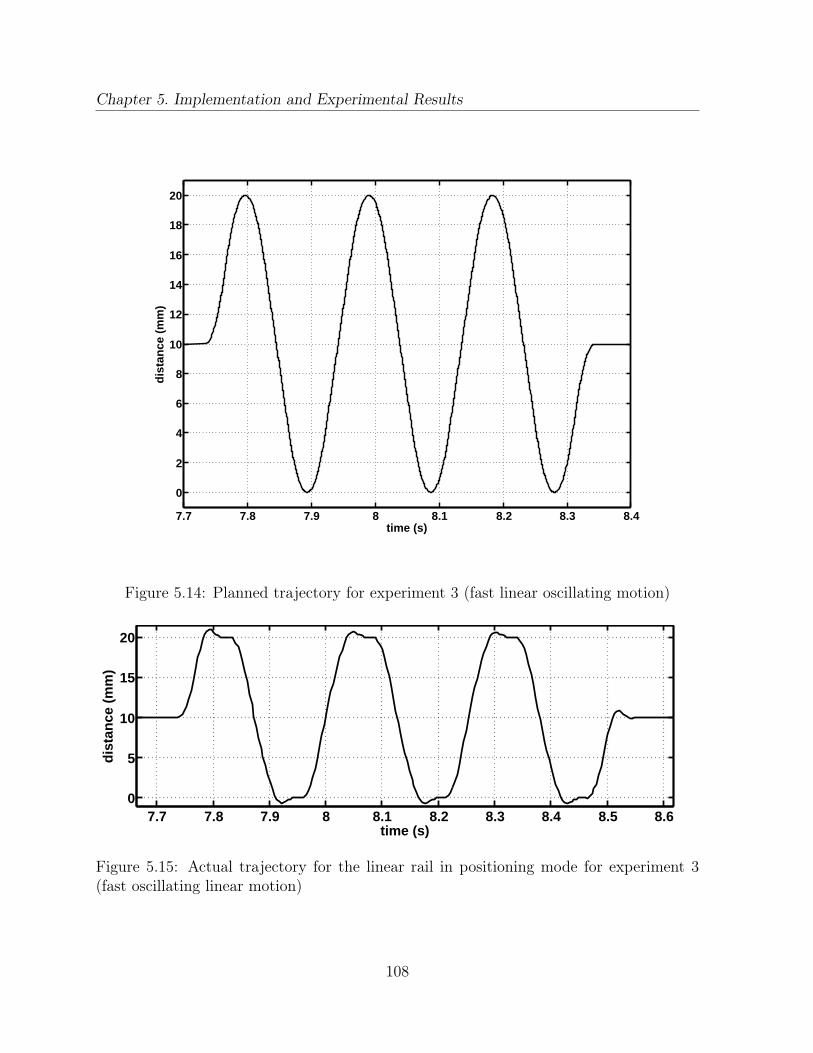
Chapter 5. Implementation and Experimental Results
7.7 7.8 7.9 8 8.1 8.2 8.3 8.4
0
2
4
6
8
10
12
14
16
18
20
time (s)
dis
tan
ce (
mm
)
Figure 5.14: Planned trajectory for experiment 3 (fast linear oscillating motion)
7.7 7.8 7.9 8 8.1 8.2 8.3 8.4 8.5 8.60
5
10
15
20
time (s)
dis
tan
ce (
mm
)
Figure 5.15: Actual trajectory for the linear rail in positioning mode for experiment 3(fast oscillating linear motion)
108

5.2. EXPERIMENTS
Figure 5.16: Sensor unit attached to tripod for calibration
109

Chapter 5. Implementation and Experimental Results
5.3 Results
The algorithm can be executed offline with Simulink or in real time on an xPC Target.The experimental results shown in this Section have all been obtained in real-time. Tocompare different algorithms under the same conditions, the sensor data from the real-time run was saved and then used to re-run a different algorithm with the same datasequence. Data association works correctly if the state estimation is not too far from thetruth; for this, the position has to be initialized with values which are approximately lessthan 20mm from the true position.
Most of the results in this Section were obtained with the Right-Invariant ExtendedFilter presented in Section 4.3.4.3. We chose this filter over the left-invariant one (seeSection 4.3.4.4) because it expresses all errors in camera coordinates and this seemssensible since we are interested in the Sensor Unit motion expressed in the camera frame.However, our analysis has not shown any significant difference between estimations fromthe Right or Left-Invariant EKF.
5.3.1 General Observations
5.3.1.1 Position and Orientation
Figure 5.17 shows the estimated position and the Euler angles calculated from theestimated quaternions for the static case in experiment 1. The position is compared tothe resolver measurement which shows that the RIEKF estimates the position correctly.We do not have a reference for the orientation; we can only say that the RIEKF estimatesa constant orientation which is correct.
Figures 5.18 and 5.19 show the estimated position and Euler angles resp. for thelinear motion in experiment 2. A comparison with the rail resolver measurement showsthat the RIEKF estimates the motion correctly, except for occasional small deviations atthe beginning or end of the motion. The RIEKF also detects a change in orientation, butagain we do not have a reference to compare this estimation to.
5.3.1.2 Filtering of Inertial Measurements
The RIEKF filters noisy measurements. Figures 5.20 and 5.21 show the measured inertialdata for experiment 1. All the signals are noisy and the accelerometer signals also shownumerous peaks. These peaks and most of the noise are filtered by the RIEKF in theposition and orientation as illustrated in Figure 5.17.
Figure 5.22 show the accelerometer data for experiments 2 and 3, illustrating whatkind of signals the IMU measures for these motions.
110

5.3. RESULTS
0 10 20 30 40 50 60 70 80 90 100883
883.5
884
884.5
885
X (
mm
)
resolver 250Hz, rel. to RIEKFdirect RIEKF 50/250Hz
0 10 20 30 40 50 60 70 80 90 100
−7
−6.8
−6.6
−6.4
−6.2
Y (
mm
)
0 10 20 30 40 50 60 70 80 90 100
−27.8
−27.6
−27.4
−27.2
−27
Z (
mm
)
time (s)
(a) Position: X coordinate (depth), horizontal Y coordinate, vertical Z coordinate
0 10 20 30 40 50 60 70 80 90 100
−94
−93
−92
−91
phi (
°)
0 10 20 30 40 50 60 70 80 90 10088
89
90
91
92
thet
a (°
)
0 10 20 30 40 50 60 70 80 90 100
−132
−131
−130
−129
psi (
°)
time (s)
(b) Euler angles
Figure 5.17: RIEKF estimation of position and Euler angles (calculated from estimatedquaternions) for experiment 1 (static)
111

Chapter 5. Implementation and Experimental Results
150 155 160 165
900
920
940X
(m
m)
150 155 160 165
0
20
40
60
Y (
mm
)
150 155 160 165−34
−32
−30
−28
Z (
mm
)
time (s)
resolver 250Hz, rel. to RIEKFdirect RIEKF 50/250Hz
Figure 5.18: RIEKF position estimation for experiment 2 (linear motion)
112

5.3. RESULTS
150 155 160 165
−94
−93
−92
−91
phi (
°)
150 155 160 16588
89
90
91
92
thet
a (°
)
150 155 160 165
−132
−131
−130
−129
psi (
°)
time (s)
Figure 5.19: Euler angles calculated from quaternions estimated by the RIEKF forexperiment 2 (linear motion)
0 10 20 30 40 50 60 70 80 90 1008.5
9
9.5
10
10.5accelerometer measurement X (m/s 2)
0 10 20 30 40 50 60 70 80 90 100−0.5
0
0.5
1
1.5accelerometer measurement Y (m/s 2)
0 10 20 30 40 50 60 70 80 90 100−1
−0.5
0
0.5
1
time (s)
accelerometer measurement Z (m/s 2)
Figure 5.20: Accelerometer measurements for experiment 1
113

Chapter 5. Implementation and Experimental Results
0 10 20 30 40 50 60 70 80 90 100−0.04
−0.02
0
0.02
0.04gyroscope measurement X (°/s)
0 10 20 30 40 50 60 70 80 90 100−0.05
0
0.05gyroscope measurement Y (°/s)
0 10 20 30 40 50 60 70 80 90 100−0.02
0
0.02
0.04
0.06
time (s)
gyroscope measurement Z (°/s)
Figure 5.21: Gyroscope measurements for experiment 1
5.3.1.3 Bias estimation
The estimated accelerometer and gyroscope biases should theoretically be identical tothe true biases present in the sensors. In fact, the estimated biases might also absorbparameter errors as mentioned in Section 4.4. The additional error terms can be constantor depend on the Sensor Unit position and/or orientation, implying that the estimatedbiases might change when the Sensor Unit moves although the true bias stays constant.
Figure 5.23 shows the estimated biases for an experiment in which the Sensor Unit waskept static for 150s and was then moved along the rail (several runs of the the trajectoriesfrom experiments 2 and 3). Since the accelerometer biases need longer than 150s toconverge, they have not been initialized with 0 but with their final values. The gyroscopebiases have been initialized with 0.
The gyroscope biases converge quickly and stay almost constant during the SensorUnit motions. The largest variation of about 7% occurs in the bias X. The accelerometerbiases are affected more strongly by the Sensor Unit motion. They vary by 9% for the Xaxis, by 5% for the Y axis and by 15% for the Z axis.
114

5.3. RESULTS
167.8 167.9 168 168.1 168.2 168.3 168.4 168.5 168.6 168.7 168.8−30
−20
−10
0
10
20oscillating linear motion (exp. 3)
time (s)acce
lero
met
er m
easu
rem
ents
(m
/s2 )
160 160.5 161 161.5 162 162.5 163 163.5 164 164.5 165
−5
0
5
10
slow linear motion (exp. 2)
time (s)acce
lero
met
er m
easu
rem
ents
(m
/s2 )
acc Xacc Yacc Z
acc Xacc Yacc Z
Figure 5.22: Accelerometer measurements for experiment 2 (above) and experiment 3(below)
115

Chapter 5. Implementation and Experimental Results
0 50 100 150 200 250 3000
0.05
0.1
0.15
0.2
0.25
0.3
acce
lero
met
er b
ias
(m/s
2 )
0 50 100 150 200 250 300
0
0.2
0.4
0.6
0.8
time (s)
gyro
scop
e bi
as (
°/s)
acc bias Xacc bias Yacc bias Z
gyro bias Xgyro bias Ygyro bias Z
Figure 5.23: Estimated accelerometer and gyroscope biases
116

5.3. RESULTS
Figure 5.24: Real-time execution times for direct and indirect RIEKF and direct MEKF
5.3.1.4 Latency
The real-time implementation with xPC Target permits us to study the computationalcost of a data fusion algorithm. The xPC Target application runs with a step of 1msand measures the execution time for each step, called target execution time (TET). Foran algorithm to run in real-time, the TET for each step has to be below 1ms. The TETmeasures the algorithm latency because it gives the time between a new measurementand the corresponding filter output.
Our first goal is to show that the direct approach reduces latency compared to theindirect approach. For this we implemented an indirect RIEKF and compared the TETfor the direct and indirect RIEKF.
The second goal is to show that the RIEKF presented in Section 4.3.4.3 has a smallerlatency than the MEKF from Section 4.3.3 because we consider that it is computationallyless complex since it takes into account system symmetries.
Figure 5.24 illustrates task execution times for the direct and indirect RIEKF and thedirect MEKF. The upper lines (marked "C") indicate times for corrections. The lowerlines (marked "P+I") and the intermediate points represent times for prediction andintegration steps (note that the red line for direct RIEKF is masked almost completelyby the blue line for the indirect RIEKF). The direct RIEKF yields the smallest executiontime, thus it has the lowest latency of the three algorithms. However, the differences
117

Chapter 5. Implementation and Experimental Results
between the algorithms are too small to be significant. A more precise measurementwould be necessary to evaluate latencies.
5.3.1.5 Discussion
In this Section, we made general observations about the RIEKF estimations. We showedthat the optical-inertial tracking system with the RIEKF can estimate the motion of theSensor Unit while filtering the noise inertial measurements. Gyroscope biases convergequickly and stay constant during the motion of the Sensor Unit, which is in accordancewith our model. The accelerometer biases however depend on the Sensor Unit motionwhich is probably due to parameter errors. Finally, we also studied the latency of thedirect RIEKF and compared to the indirect RIEKF and to the MEKF.
5.3.2 Precision and Accuracy
Measurement systems are often evaluated regarding their precision and accuracy, andthese terms are also applied to indirect measurements where values are obtainedby some computation from measured data [Miller et al., 2009]. Precision is the de-gree to which repeated measurements under unchanged conditions show the sameresults [Miller et al., 2009]. For our optical-inertial tracking system for example, we wouldlike to study the precision of the position estimation, that is by how the estimated positionvaries when the true position is constant. Accuracy describes how close a measurement isto its true value [Miller et al., 2009]. In our case, accuracy describes whether the estimatedposition is equal to the true position or whether it is offset by a systematic error.
5.3.2.1 Precision (static case)
We study the precision using data from experiment 1 (static case) from t=10s to t=100s(we leave out the first 10s because the filter has not converged yet during this time).Figure 5.17(a) shows the position estimationand Figure 5.17(b) the Euler angles calculatedfrom the estimated quaternions.
The position has the following mean and standard deviation:
C p =⎡⎢⎢⎢⎢⎢⎣
884.1436−6.6690−27.3574
⎤⎥⎥⎥⎥⎥⎦mm std(C p) =
⎡⎢⎢⎢⎢⎢⎣
0.09960.04520.0404
⎤⎥⎥⎥⎥⎥⎦mm .
The position varies from
C pmin =⎡⎢⎢⎢⎢⎢⎣
883.8088−6.8435−27.5295
⎤⎥⎥⎥⎥⎥⎦mm to C pmax =
⎡⎢⎢⎢⎢⎢⎣
884.4879−6.4642−27.1763
⎤⎥⎥⎥⎥⎥⎦mm
118

5.3. RESULTS
which gives a difference of
∆C p =⎡⎢⎢⎢⎢⎢⎣
0.67900.37940.3532
⎤⎥⎥⎥⎥⎥⎦mm .
Both the standard deviation and the difference between minimum and maximum valuesshow that the precision is approximately the same in Y and Z and that it is twice as goodin these directions than depth precision (coordinate X).
The angles have the following mean and standard deviation:
⎡⎢⎢⎢⎢⎢⎣
φ
θ
ψ
⎤⎥⎥⎥⎥⎥⎦=⎡⎢⎢⎢⎢⎢⎣
−1.61961.5756−2.2812
⎤⎥⎥⎥⎥⎥⎦degrees std(
⎡⎢⎢⎢⎢⎢⎣
φθψ
⎤⎥⎥⎥⎥⎥⎦) =
⎡⎢⎢⎢⎢⎢⎣
0.3628 ⋅ 10−3
0.6661 ⋅ 10−3
0.5064 ⋅ 10−3
⎤⎥⎥⎥⎥⎥⎦degrees .
The angles vary from
⎡⎢⎢⎢⎢⎢⎣
φθψ
⎤⎥⎥⎥⎥⎥⎦min=⎡⎢⎢⎢⎢⎢⎣
−1.62081.5735−2.2825
⎤⎥⎥⎥⎥⎥⎦degrees to
⎡⎢⎢⎢⎢⎢⎣
φθψ
⎤⎥⎥⎥⎥⎥⎦max=⎡⎢⎢⎢⎢⎢⎣
−1.61851.5774−2.2793
⎤⎥⎥⎥⎥⎥⎦degrees
which gives a difference of⎡⎢⎢⎢⎢⎢⎣
∆φ∆θ∆ψ
⎤⎥⎥⎥⎥⎥⎦=⎡⎢⎢⎢⎢⎢⎣
0.00230.00380.0032
⎤⎥⎥⎥⎥⎥⎦degrees .
5.3.2.2 Accuracy
Since we do not have an absolute reference for the Sensor Unit position and orientation,we cannot evaluate the accuracy of the optical-inertial system with the RIEKF.
5.3.3 High-Bandwidth Tracking
Figures 5.25-5.27 show the position estimated by the RIEKF (with an optical frequencyof 50Hz and an inertial frequency of 250Hz) for two repeats of the oscillation with 1cmamplitude during experiment 3. Figure 5.25 depicts the X coordinate (which representsdepth), Figure 5.26 the horizontal Y coordinate and Figure 5.25 the vertical Z coordinateof the position. The RIEKF follows the oscillating motion well. There are a few deviations,namely at the points where the rail carriage changes direction. At these inversions, theremight be a problem with the resolver measurement which is used as ground truth. Sinceit is only an indirect measurement counting the number of turns of the motor, it possiblydoes not give the correct value at inversions due to transmission errors. Thus we cannot
119

Chapter 5. Implementation and Experimental Results
167.8 168 168.2 168.4 168.6 168.8 169
882
884
886
888
890
892
894
896
time (s)
X (m
m)
resolver 250Hz, rel. to RIEKFoptical 50Hzdirect RIEKF 50/250Hz
(a) first run
184.2 184.4 184.6 184.8 185 185.2
882
884
886
888
890
892
894
896
time (s)
X (m
m)
resolver 250Hz, rel. to RIEKFoptical 50Hzdirect RIEKF 50/250Hz
(b) second run
Figure 5.25: X position coordinate for oscillation in experiment 3
120
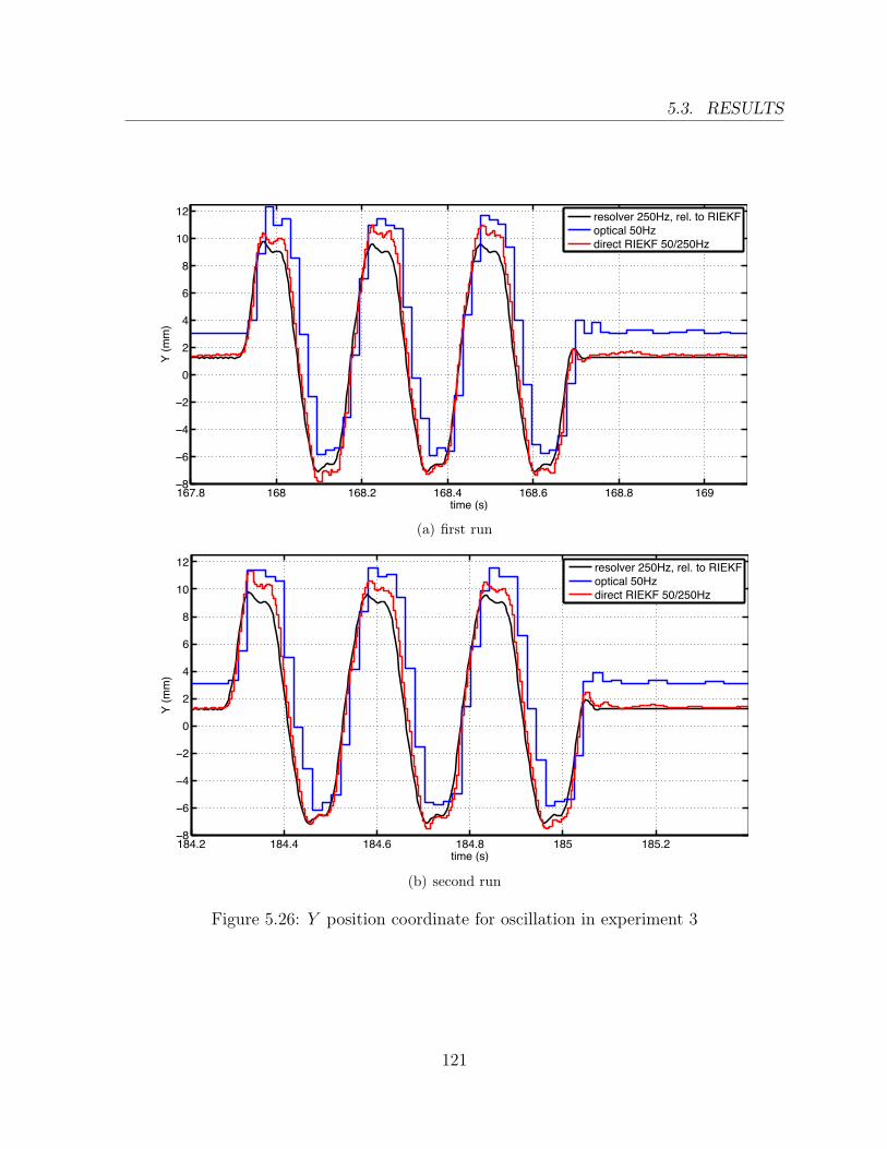
5.3. RESULTS
167.8 168 168.2 168.4 168.6 168.8 169−8
−6
−4
−2
0
2
4
6
8
10
12
time (s)
Y (m
m)
resolver 250Hz, rel. to RIEKFoptical 50Hzdirect RIEKF 50/250Hz
(a) first run
184.2 184.4 184.6 184.8 185 185.2−8
−6
−4
−2
0
2
4
6
8
10
12
time (s)
Y (m
m)
resolver 250Hz, rel. to RIEKFoptical 50Hzdirect RIEKF 50/250Hz
(b) second run
Figure 5.26: Y position coordinate for oscillation in experiment 3
121
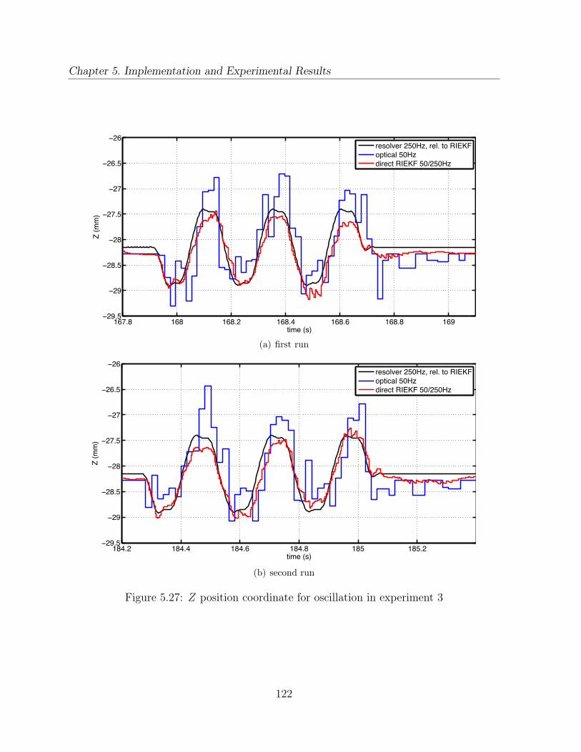
Chapter 5. Implementation and Experimental Results
167.8 168 168.2 168.4 168.6 168.8 169−29.5
−29
−28.5
−28
−27.5
−27
−26.5
−26
time (s)
Z (m
m)
resolver 250Hz, rel. to RIEKFoptical 50Hzdirect RIEKF 50/250Hz
(a) first run
184.2 184.4 184.6 184.8 185 185.2−29.5
−29
−28.5
−28
−27.5
−27
−26.5
−26
time (s)
Z (m
m)
resolver 250Hz, rel. to RIEKFoptical 50Hzdirect RIEKF 50/250Hz
(b) second run
Figure 5.27: Z position coordinate for oscillation in experiment 3
122

5.3. RESULTS
167.8 167.9 168 168.1 168.2 168.3 168.4 168.5 168.6 168.7 168.8
−94
−93
−92
−91ph
i (°)
167.8 167.9 168 168.1 168.2 168.3 168.4 168.5 168.6 168.7 168.888
89
90
91
92
thet
a (°
)
167.8 167.9 168 168.1 168.2 168.3 168.4 168.5 168.6 168.7 168.8−131
−130
−129
−128
−127
psi (
°)
time (s)
direct RIEKF 50/250Hzoptical 50Hz
Figure 5.28: Angles for oscillation in experiment 3
judge the RIEKF estimation at these points because we might not have a correct groundtruth.
Having compared the RIEKF estimation to the rail reference, we next look at itin contrast to optical tracking. The optical position is determined as described inSection 5.1.6.2 and plotted in Figures 5.25-5.27. We start by examining the Y coordinatein Figure 5.26 which is the axis in which most of the motion took place. The opticalposition gives only a very imprecise approximation of this curve. This is even moreevident when looking at the Z coordinate in Figure 5.27. The Sensor Unit moved byonly approximately 1.5mm in this axis and the optical system does not see this motioncorrectly. This shows that the optical-inertial tracking system with its high bandwidth ismore suitable than an optical tracking system to follow fast motion.
Figure 5.28 illustrate the Euler angles estimated by the RIEKF and from opticaltracking for the 1cm oscillation in experiment 3. We cannot judge the accuracy of thisestimation since we do not have a reference but the optical Euler angles obviously display
123

Chapter 5. Implementation and Experimental Results
167.8 167.9 168 168.1 168.2 168.3 168.4 168.5 168.6 168.7 168.8880
882
884
886
888
890
892
894
896
898
time (s)
X (
mm
)
resolver 250Hz, rel. to RIEKFoptical 12.5Hzdirect RIEKF 12.5/250Hz
Figure 5.29: X position coordinate for oscillation in exp. 3 with an optical rate of 12.5Hz
sudden changes which is not correct.Having determined that the optical-inertial tracking system with an inertial sample
rate of 250Hz and an optical sample rate of 50Hz can in fact follow the fast motionof the Sensor Unit we would now like to study if it is possible to further augment thesystem bandwidth. The experimental setup described in Section 5.1 does not permit usto increase the inertial sample rate beyond 250Hz. Augmenting the inertial rate meansaugmenting the number of predictions between two corrections. Since we cannot increasethe inertial rate we lower the optical rate to 12.5Hz instead. This gives a factor of 20between the optical and inertia sensor rates and consequently 20 predictions are executedin the RIEKF between two corrections. Figures 5.29-5.31 show the position estimationfrom the RIEKF and optical tracking for this case. The RIEKF estimation is of courseless good than for the case of a 50Hz optical rate, but it still detects the oscillating motionand does so much better than the optical tracking.
5.3.4 Influence of Sensor Unit Calibration
In Section 4.4.1.1 we studied the influence of Marker-Body transformation errors onthe RIEKF estimation in theory. Now we look at the effect of a change of Marker-Body transformation on the RIEKF estimations obtained from real data and will
124

5.3. RESULTS
167.8 167.9 168 168.1 168.2 168.3 168.4 168.5 168.6 168.7 168.8−10
−5
0
5
10
15
time (s)
Y (
mm
)
resolver 250Hz, rel. to RIEKFoptical 12.5Hzdirect RIEKF 12.5/250Hz
Figure 5.30: Y position coordinate for oscillation in exp. 3 with an optical rate of 12.5Hz
167.8 167.9 168 168.1 168.2 168.3 168.4 168.5 168.6 168.7 168.8−30
−29.5
−29
−28.5
−28
−27.5
−27
time (s)
Z (
mm
)
resolver 250Hz, rel. to RIEKFoptical 12.5Hzdirect RIEKF 12.5/250Hz
Figure 5.31: Z position coordinate for oscillation in exp. 3 with an optical rate of 12.5Hz
125

Chapter 5. Implementation and Experimental Results
10 20 30 40 50 60 70 80 90 100
−4.02−4.01
−4−3.99−3.98
X (
mm
)
10 20 30 40 50 60 70 80 90 100
9.9
9.91
9.92
9.93
Y (
mm
)
10 20 30 40 50 60 70 80 90 1005.82
5.84
5.86
5.88
Z (
mm
)
time (s)
∆ p between case with Bd=[6.0429,−4.6087,9.5305] T and Bd=0− R(q) ∆ Bd
Figure 5.32: Difference of the position estimated with Bd = [6.0429,−4.6087,9.5305]T andBd = 0 (blue), and error −R(BC q)∆Bd as calculated in the error analysis (red), static case
see that the theoretical values are confirmed. We compare the case of the markermodel measured with a ruler (here, Bd = 0 and MBR = I3) and that with a Marker-Body transformation determined from calibration procedures. The different models aredescribed in Section 5.4.4.
We start by looking at the effect of a change of the translation vector. Using differenttranslation vectors Bd leads to a translation in the estimated Sensor Unit position asdetermined in the error analysis in Section 4.4.1.1. Figure 5.33 plots the difference betweentwo positions for experiment 1, one estimated with
Bd = [6.0429,−4.6087,9.5305]T
and the other with Bd = 0. This figure also shows the term −R(BC q)∆Bd where ∆Bd is thedifference between the two translation vectors considered here. The term −R(BC q)∆Bdis the one given in Equation (4.78) for a translation error ∆Bd. Since both curves overlapafter the initialization phase, this illustrates that the theoretical result from the erroranalysis is confirmed when using experimental data. The error analysis was done forsteady-state and consequently it is only true for the static case. This is illustrated inFigure 5.33 where the same variables are shown for the oscillating motion in experiment 3:in this non-static case, the two variables are not equal.
126

5.3. RESULTS
167.8 167.9 168 168.1 168.2 168.3 168.4 168.5 168.6 168.7 168.8−4.07
−4.06
−4.05
−4.04
−4.03
X (
mm
)
167.8 167.9 168 168.1 168.2 168.3 168.4 168.5 168.6 168.7 168.89.83
9.84
9.85
9.86
9.87
Y (
mm
)
167.8 167.9 168 168.1 168.2 168.3 168.4 168.5 168.6 168.7 168.85.88
5.9
5.92
5.94
5.96
Z (
mm
)
time (s)
∆ p between case with Bd=[6.0429,−4.6087,9.5305] T and Bd=0− R(q) ∆ Bd
Figure 5.33: Difference of the position estimated with Bd = [6.0429,−4.6087,9.5305]T andBd = 0 (blue), and error −R(BC q)∆Bd as calculated in the error analysis (red), duringmotion
127

Chapter 5. Implementation and Experimental Results
We now move on the effect of the Marker-Body rotation matrix. Two differentrotation matrices MBR lead to small changes in position and orientation as given inEquations (4.78) and (4.80). The main difference lies in the estimated accelerometerbiases which will be illustrated in Section 5.4.4.2 about the calibration of the Marker-Body rotation.
5.4 Calibration
5.4.1 Optical System
Regarding the calibration of the optical system, we have to determine the camera intrinsicvalues, the rotation between the world and camera frame and the transformation betweenthe two stereo cameras.
The optical system has to be calibrated only once since its parameters are constant.The rotation between world and camera frame and the stereo transformation have to bere-calibrated when the setup has been changed.
5.4.1.1 Camera
Each camera is calibrated using the method presented in Section 3.3.1 and a planarcalibration target consisting of four LEDs. This gives the camera’s intrinsic parameters.
For the left camera, we obtained
fu,L = 1366.2208, fv,L = 1368.8532, SuL = [542.6768, 366.07549]T
and for the right camera
fu,R = 1366.5736, fv,R = 1358.715, SuR = [531.61743, 360.94375]T .
All the parameters are in pixels.
Rotation between world and camera frame The orientation WCq of the cameraframe C with respect to the world frame W has to be known in order to calculateCG = WCq ∗WG ∗WCq−1 in the differential equation for the Sensor Unit velocity (2.8).We chose the following procedure to determine WCq.
1 The Sensor Unit is placed in such a way in front of the cameras that the marker planeis aligned with the vertical axis.
2 The orientation BCq is calculated using optical data.
128

5.4. CALIBRATION
3 Since the world and marker frames are aligned, the rotation matrix
Mp = WMRWp
can be determined easily; the quaternion WMq is then deduced from WMR.
4 WCq can then be calculated from BCq :
WCq = BCq ∗MBq ∗WMq
where the rotation MBq between marker and body frame has been determined bycalibration (see Sensor Unit Calibration below).
5.4.1.2 Stereo rig
The stereo rig is calibrated according to the method [Bouguet, 2010] as described inSection 3.3.1.1. The procedure yielded the following stereo transformation:
RSt =⎡⎢⎢⎢⎢⎢⎣
0.9698 −0.2421 −0.02830.2410 0.9698 −0.03660.0363 0.0287 0.9989
⎤⎥⎥⎥⎥⎥⎦, tSt =
⎡⎢⎢⎢⎢⎢⎣
42.7094−374.9868−2.4414
⎤⎥⎥⎥⎥⎥⎦mm
5.4.2 Accelerometers
Axis misalignment, scale factors and biases were calibrated with an iterative algorithm[Dorveaux et al., 2009] as described in Section 3.3.2.
For one calibration procedure we obtained a matrix
A =⎡⎢⎢⎢⎢⎢⎣
1.0003 −0.0022 −0.00010.0032 0.9997 −0.00080.0006 0.0011 0.9977
⎤⎥⎥⎥⎥⎥⎦
containing scale factor and misalignments and a bias vector
B =⎡⎢⎢⎢⎢⎢⎣
32.2661668.485670.2366
⎤⎥⎥⎥⎥⎥⎦
mm
s2.
Note that these values might change every time the sensors are turned on.
129

Chapter 5. Implementation and Experimental Results
5.4.3 Gyroscopes
Regarding the gyroscopes, we do not consider scales or misalignment but only biases. Thebias consists of a constant part ωb and a term depending on the specific acceleration, calledg-dependent bias [Groves, 2008]: Bg
Ba. Most of this g-dependent bias can be compensatedin the IMU used here [ADIS16355, 2009], but a small dependency remains. To determinethe constant bias term ωb, the Sensor Unit is rotated into several different orientationsand then kept static for several second. The gyroscope measurements are averaged over10s to give ωi for each orientation i. Accelerometer measurements are compensated formisalignment, scale factors and biases as described in the previous Section and averagedover 10s to give ai. The g-dependent bias matrix Bg and the gyroscope bias are calculatedusing linear least squares:
Bgai + ωb = ωi
⇔⎡⎢⎢⎢⎢⎢⎣
g1g2g3
⎤⎥⎥⎥⎥⎥⎦ai + ωb = ωi
⇔⎡⎢⎢⎢⎢⎢⎣
aTi 0 0 ∥0 aTi 0 ∥ I30 0 aTi ∥
⎤⎥⎥⎥⎥⎥⎦
⎡⎢⎢⎢⎢⎢⎢⎢⎣
g1T
g2T
g3T
ωb
⎤⎥⎥⎥⎥⎥⎥⎥⎦
= ωi
5.4.4 Sensor Unit
The calibration of the Sensor Unit consists in determining the optical marker positions inthe Body frame which is the frame of the inertial sensors. In a first step, the positions weremeasured with a ruler as given in Section 5.4.4.1. These measurements are inaccurate dueto two reasons: Firstly, it was impossible to perfectly align the IMU and the circuit boardcontaining the optical markers. Secondly, the center of the IMU frame inside the casingis not given in the datasheet and could only be estimated. This explains the need for acalibration of the Marker-Body transformation as described in Section 5.4.4.2.
The marker model and the Marker-Body transformation have to be determined onlyonce since they only depend on the Sensor Unit geometry and are constant.
5.4.4.1 Marker Model
Positions Mmi are measured with a ruler:
[Mm1Mm2
Mm3Mm4] =
⎡⎢⎢⎢⎢⎢⎣
−30 48.5 31 −122−63.5 −63.5 78.5 78.5−58 −58 −58 −60
⎤⎥⎥⎥⎥⎥⎦mm
130

5.4. CALIBRATION
0 100 200 300 400 500 600 700 800−1500
−1000
−500
0
500
1000accelerometer bias estimation
(mm
/s2 )
0 100 200 300 400 500 600 700 800−0.2
0
0.2
0.4
0.6
0.8
1
1.2gyro bias estimation
time (s)
(°/s
)
acc x with MBR=Iacc yacc zacc x with new MBRacc yacc z
gyro bias xgyro bias ygyro bias zmean gyro xmean gyro ymean gyro z
Figure 5.34: Estimated accelerometer biases for different orientations, with MBR = I (solidlines) and with MBR from calibration (dashed lines).
5.4.4.2 Marker-Body Transformation
The Marker-Body transformation (MBR, Bd) has to be known in order to transform themarker model to body coordinates:
Bmi = MBRMmi + Bd
Estimation as Additional State in the RIEKF We adapted the idea of adding thetransformation as additional states as presented in [Mirzaei and Roumeliotis, 2008] to theoutside-in case. That is we added the quaternion MBq and Bd to the state of the systemto be estimated and changed the RIEKF accordingly. But this filter did not convergeeither in simulation or with real data.
Method Using RIEKF Bias Estimates The Marker-Body rotation was estimatedwith the method described in Section 4.4.2. For this calibration, the Sensor Unit wasrotated into seven different orientation as described in Section 5.2.4. For each orientation,the system state was estimated using the RIEKF. The measured calibrated accelerometermeasurements and the estimated accelerometer biases were then averaged over 10s to giveam and Bab which are the values used in the calibration procedure.
The Marker-Body rotation found through this calibration isMBq = [0.9987 − 0.0079 0.0478 − 0.0143]
which gives a rotation matrix
MBR =⎡⎢⎢⎢⎢⎢⎣
0.9950 0.0277 0.0959−0.0292 0.9995 0.0146−0.0954 −0.0173 0.9953
⎤⎥⎥⎥⎥⎥⎦
131
Chapter 5. Implementation and Experimental Results
Figure 5.34 shows the biases estimated by the RIEKF for the 7 different static orientationsfor MBR = I (before calibration) and for the matrix MBR determined by calibration usingthese 7 orientations. In call cases, "calibrated" accelerometer measurements have beenused in which the biases have been removed; thus the biases estimated by the RIEKFshould be zero.
Firstly, we see that the estimated biases depend on the orientation which is dueto parameter errors as discussed in Section 4.4.1. Obviously, the goal of calibrationprocedures would be to eliminate these errors from the model in order to remove parametererror terms from the accelerometer biases. With correct parameters, the estimated biaseswould be equal to the true sensor biases. Secondly, and most importantly, the Figureshows that with the calibrated MBR, the biases are reduced for almost all orientations.They are not equal to zero, probably due to other calibration errors which have not yetbeen compensated, but this result still shows the positive effect of this calibration method.
Least Squares Approach Using Optical Measurements We adapted the calibra-tion in [Kim and Golnaraghi, 2004] which uses pose information from an optical trackingsystem as ground truth. [Kim and Golnaraghi, 2004] estimates biases, gains and axesmisalignments for a triad of gyroscopes and accelerometers. We use this approach toestimate the transformation only because biases, gains and misalignments have alreadybeen compensated for by the accelerometer calibration.
The marker positions are determined by triangulation:Cmi =Cp + BCq ∗ Bmi ∗ BCq−1
=Cp + BCq ∗ Bd ∗ BCq−1
´¹¹¹¹¹¹¹¹¹¹¹¹¹¹¹¹¹¹¹¹¹¹¹¹¹¹¹¹¹¹¹¹¹¹¹¹¹¹¹¹¹¹¹¹¹¹¹¹¹¹¹¹¹¹¹¹¹¹¹¹¹¹¹¹¸¹¹¹¹¹¹¹¹¹¹¹¹¹¹¹¹¹¹¹¹¹¹¹¹¹¹¹¹¹¹¹¹¹¹¹¹¹¹¹¹¹¹¹¹¹¹¹¹¹¹¹¹¹¹¹¹¹¹¹¹¹¹¹¹¶=∶Cr
+ (BCq ∗MBq)´¹¹¹¹¹¹¹¹¹¹¹¹¹¹¹¹¹¹¹¹¹¹¹¹¹¹¹¹¹¸¹¹¹¹¹¹¹¹¹¹¹¹¹¹¹¹¹¹¹¹¹¹¹¹¹¹¹¹¹
=∶MCq
∗Mmi ∗ (BCq ∗MBq)−1
Cr is the origin of the marker frame in camera coordinates and MCq is the Marker-bodyrotation. Cr and MCq are determined by one of the solutions of the Absolute OrientationProblem (see Section 3.1.2.2), in our case by Walker’s method [Walker et al., 1991].
We differentiate the Marker-Camera quaternion to get the angular velocity:
MC q =BC q ∗MBq = 1
2BCq ∗ ω ∗MBq
=1
2MCq ∗MBq−1 ∗ ω ∗MBq
⇔ ω =2MBq ∗MCq−1 ∗MC q ∗MBq−1
and we differentiate ω to get ω:
ω =2MBq ∗ (MCq−1 ∗MC q −MCq−1 ∗MC q ∗MCq−1 ∗MC q) ∗MBq−1
=2MBq−1 ∗MCq−1 ∗ (MC q −MC q ∗MCq−1 ∗MC q) ∗MBq
132

5.4. CALIBRATION
The position Cr is now derived twice to obtain the acceleration:
C r =C p + BCq ∗ (ω × (ω × Bd) + ω × Bd) ∗ BCq−1
=CG +MCq ∗MBq−1 ∗ (a + ω × (ω × Bd) + ω × Bd) ∗MBq ∗MCq−1
⇔ a =MBq ∗MCq−1 ∗ (C r − CG) ∗MCq ∗MBq−1 − ω × (ω × Bd) − ω × Bd
We have now expressed ω and a as functions of the measured optical position andorientation and their derivatives and of the transformation (Bd,MBq).
The rotation MBq has been determined in the previous Section and does not need tobe re-estimated here. In this case, the equation for the specific acceleration is linear inBd and can be written as
([ω]×[ω]× + [ω]×)Bd = −a +MBq ∗MCq−1 ∗ (C r − CG) ∗MCq ∗MBq−1
This equation is written for each frame. We obtain an overdetermined linear system whichwill be of rank 3 if ω and ω are different from zero and vary from frame to frame. Thesolution of this system will give the translation vector Bd.
The necessary IMU and optical measurements are obtained from a calibration routineduring which the Sensor Unit is moved in front of the stereo camera rig. The opticalmeasurements give Cr and MCq. The accelerometer measurements are "calibrated" (i.e.biases, gains and misalignments are compensated for) to give a for each frame.
This calibration procedure yielded the following translation vector:
Bd =⎡⎢⎢⎢⎢⎢⎣
6.0429−4.60879.5305
⎤⎥⎥⎥⎥⎥⎦mm
5.4.4.3 Final Sensor Unit Model
The marker coordinates in Body coordinates after calibration read:
Bmi = MBRMmi + Bd
with
MBR =⎡⎢⎢⎢⎢⎢⎣
0.9950 0.0277 0.0959−0.0292 0.9995 0.0146−0.0954 −0.0173 0.9953
⎤⎥⎥⎥⎥⎥⎦and
Bd =⎡⎢⎢⎢⎢⎢⎣
6.0429−4.60879.5305
⎤⎥⎥⎥⎥⎥⎦mm
133

Chapter 5. Implementation and Experimental Results
which gives
[Bm1Bm2
Bm3Bm4] =
⎡⎢⎢⎢⎢⎢⎣
−31.1281 46.9800 33.5022 −118.9256−68.0422 −70.3373 72.0986 76.5428−44.2353 −51.7264 −52.5117 −39.9018
⎤⎥⎥⎥⎥⎥⎦mm .
134

Chapter 6
Conclusion
Dans cette thèse, nous avons présenté un système de tracking qui utilise des capteursoptiques et inertiels pour déterminer la position et l’orientation d’une Sensor Unit. Letracking a une grande bande passante d’au moins 200Hz et un petit temps de latence.
Le système permet de suivre un outil à main dans un système de chirurgie assistée parordinateur. Grâce au tracking, l’outil peut être asservi pour rester dans un plan ou surune trajectoire.
Le cœur du système est un algorithme de fusion de données qui intègre les donnéesdes différents capteurs pour déterminer la position et l’orientation de la Sensor Unit. Ila une grande bande passante car il tourne à la fréquence élevée des capteurs inertiels. Lefiltre repose sur une approche directe utilisant des données brutes pour réduire le temps decalcul et il prend en compte les symmétries du système.
L’implémentation en temps réel avec un dispositif expérimental avec des caméras etdes capteurs inertiels a permis de montrer que le tracking optique-inertiel peut en effetsuivre un objet en mouvement avec une grande bande passante. Nous suggérons plusieursaméliorations pour les versions futures du dispositif expérimental.
In this work, we presented an optical-inertial tracking system. It consists of twostationary cameras and a Sensor Unit with optical markers and an inertial measurementunit. This Sensor Unit is attached to the object being tracked.
The tracking system was developed with an application in a computer-assisted surgerysystem in mind. The goal is to track a handheld tool and to servo-control it to make itstay in a desired plane or make it move along a desired trajectory. The fact of using thetracking for servo-control introduces two main requirements which are not met by theoptical tracking systems currently used for computer-assisted surgery. The system hasto have a high bandwidth of at least 200Hz and a low latency, i.e. the delay betweena measurement and the tracking output has to be small. Our optical-inertial trackingsystem meets these requirements. Optical tracking systems used today have a bandwidth
135
Chapter 6. Conclusion
of 60Hz. Faster systems exist but are too expensive for applications in computer-assistedsurgery. Even if the cost for faster systems were to be reduced in the future, an optical-inertial tracking system like the one we propose would always be less expensive due tothe low cost of the inertial sensors. Also, the use of inertial sensors has the advantages ofimproving disturbance rejection which is important for servo-control.
The heart of the optical-inertial tracking system is the data fusion algorithm whichintegrates data from the different sensors, that is optical data from the cameras andinertial data from accelerometers and gyroscopes. It uses a mathematical model of thesystem dynamics and output. The algorithm runs at the inertial sensor frequency of200Hz or more which ensures high-bandwidth tracking. In order to reduce latency, wepropose a direct approach using sensor data directly in the filter without any previouscomputations and we also present algorithms taking into account system symmetries andthereby reducing the computational complexity. They are called Right-Invariant andLeft-Invariant Extended Kalman Filters. This low-latency approach presents the mostimportant distinction of our system from others presented in the literature.
Calibration of individual sensors and of the optical-inertial setup is important forthe system performance. Since the inertial sensors are used to provide high-bandwidthinformation, they have to be correctly calibrated because the tracking depends solely onthe inertial data and the system model between two optical measurements. Determinationof the relation between optical markers and the IMU in the Sensor Unit also turned outto be crucial to the system performance. We proposed a novel method to determine therotation between the optical markers and the IMU using estimations from our data fusionalgorithm.
To test the proposed data fusion algorithms, we developed an experimental setup withimages sensors from the Wiimote and an IMU. Sensor data was read by a microcontrollerat 50Hz from the cameras and at 250Hz from the inertial sensors. The algorithms wereimplemented in Simulink and executed in real time with an xPC Target application. Toevaluate the performance, estimations from the optical-inertial system were comparedto resolver measurements from a linear rail and to optical tracking. Experiments withmovements executed by the linear rail show that our system can track the movementscorrectly and with a high bandwidth.
In the future, the experimental setup would have to be improved to make a moreaccurate evaluation possible. The cameras would have to be replaced by more performingones which can see more than four points and would thus be able to track more thanone object. In the final application, the handheld tool has to be tracked relative to thepatient, requiring at least two rigid bodies with optical markers attached to the patient.In the OrthoPilot [Aesculap AG, 2011], for example, three rigid bodies are currently used:on attached to the tibia, on to the femur and one which can be fixed to the foot or toan instrument. The size of the Sensor Unit could also be reduced because it is currently
136

needlessly large. In order to provide real-time tracking, the data transmission speed shouldbe increased.
Ultimately, the goal is to test the tracking system with a servo-controlled tool in orderto evaluate its performance.
137


Bibliography
[ADIS16355, 2009] ADIS16355 (2009). ADIS16350/ADIS16355 data sheet, rev. B. AnalogDevices (Norwood, MA,USA).
[advanced realtime tracking GmbH, 2011] advanced realtime tracking GmbH (2011).Weilheim, Germany. http://www.ar-tracking.de/.
[Aesculap AG, 2011] Aesculap AG (2011). Tuttlingen, Germany. http://www.orthopilot.de/.
[Allan, 1966] Allan, D. (1966). Statistics of atomic frequency standards. Proceedings ofthe IEEE, 54(2):221 – 230.
[Ang et al., 2004] Ang, W. T., Khosla, P. K., and Riviere, C. N. (2004). Kalman filteringfor real-time orientation tracking of handheld microsurgical instrument. In Proceedingsof 2004 IEEE/RSJ International Conference on Intelligent Robots and Systems, pages2574–2580, Sendai, Japan.
[ATmega2560, 2007] ATmega2560 (2007). Data sheet, Rev. 2549L-08/07. AtmelCorporation, San Jose, CA, USA.
[Besancon, 2007] Besancon, G. (2007). Nonlinear Observers and Applications, vol-ume 363/2007 of Lecture Notes in Control and Information Sciences. SpringerBerlin/Heidelberg.
[Bleser and Stricker, 2008] Bleser, G. and Stricker, D. (2008). Advanced tracking throughefficient image processing and visual-inertial sensor fusion. In IEEE Virtual RealityConference (VR), pages 137–144.
[Bonnabel et al., 2008] Bonnabel, S., Martin, P., and Rouchon, P. (2008). Symmetry-preserving observers. IEEE Transactions on Automatic Control, 53(11):2514–2526.
[Bonnabel et al., 2009] Bonnabel, S., Martin, P., and Salaün, E. (2009). Invariantextended Kalman filter: theory and application to a velocity-aided attitude estimationproblem. In Proceedings of the 48th IEEE Conference on Decision and Control.
139

BIBLIOGRAPHY
[Bouguet, 2010] Bouguet, J.-Y. (2010). Camera calibration toolbox for Matlab. http://www.vision.caltech.edu/bouguetj/calib_doc.
[Brisson et al., 2004] Brisson, G., Kanade, T., Gioia, A. M. D., and Jaramaz, B. (2004).Precision freehand sculpting of bone. In Medical Image Computing and Computer-Assisted Intervention (MICCAI), volume 3217 of LNCS, pages 105 – 112. SpringerBerlin / Heidelberg.
[Cartiaux et al., 2010] Cartiaux, O., Paul, L., Docquier, P. L., Raucent, B., Dombre, E.,and Banse, X. (2010). Computer-assisted and robot-assisted technologies to improvebone-cutting accuracy when integrated with a freehand process using an oscillatingsaw. Journal of Bone and Joint Surgery - Series A, 92(11):2076–2082.
[Chum et al., 2005] Chum, O., Pajdla, T., and Sturm, P. (2005). The geometric error forhomographies. Computer Vision and Image Understanding, 97(1):86–102.
[Crassidis et al., 2007] Crassidis, J. L., Markley, F. L., and Cheng, Y. (2007). Survey ofnonlinear attitude estimation methods. Journal of Guidance, Control, and Dynamics,30(1):12–28.
[Davies, 1996] Davies, B. L. (1996). Computer-Integrated Surgery, chapter 19, pages 287–296. MIT Press, Boston, Massachusetts.
[DeMenthon et al., 2001] DeMenthon, D., David, P., and Samet, H. (2001). SoftPOSIT:An algorithm for registration of 3D models to noisy perspective images combiningSoftassign and POSIT. Technical report car-tr-969, cs-tr-4257, Center for AutomationResearch, University of Maryland, College Park, MD.
[DiGioia et al., 2004] DiGioia, A. M., Jaramaz, B., Picard, F., and Nolte, L.-P., editors(2004). Computer and Robotic Assisted Knee and Hip Surgery. Oxford University Press.
[Dorveaux et al., 2009] Dorveaux, E., Vissière, D., Martin, A.-P., and Petit, N. (2009).Iterative calibration method for inertial and magnetic sensors. In IEEE Conference onDecision and Control and 28th Chinese Control Conference.
[Eggert et al., 1997] Eggert, D., Lorusso, A., and Fisher, R. (1997). Estimating 3-D rigidbody transformations: a comparison of four major algorithms. Machine Vision andApplications, 9:272–290.
[Farrel and Barth, 1998] Farrel, J. A. and Barth, M. (1998). The Global PositioningSystem and Inertial Navigation. McGraw-Hill Companies, Inc.
140

BIBLIOGRAPHY
[Fischler and Bolles, 1981] Fischler, M. A. and Bolles, R. C. (1981). Random sampleconsensus: a paradigm for model fitting with applications to image analysis andautomated cartography. Communications of the ACM, 24(6):381–395.
[Follmann et al., 2010] Follmann, A., Korff, A., Fürtjes, T., Lauer, W., Kunze, S.,Schmieder, K., and Radermacher, K. (2010). Evaluation of a synergistically controlledsemiautomatic trepanation system for neurosurgery. In 2010 Annual InternationalConference of the IEEE Engineering in Medicine and Biology Society (EMBC), pages2304 –2307.
[Fong et al., 2008] Fong, W. T., Ong, S. K., and Nee, A. Y. C. (2008). Methods forin-field user calibration of an inertial measurement unit without external equipment.Measurement Science and Technology, 19(8):085202.
[Gebre-Egziabher, 2004] Gebre-Egziabher, D. (2004). Design and Performance Analysisof a Low-Cost Aided Dead Reckoning Navigator. PhD thesis, Standford University.
[Gebre-Egziabher et al., 2004] Gebre-Egziabher, D., Hayward, R., and Powell, J. (2004).Design of multi-sensor attitude determination systems. IEEE Transactions onAerospace and Electronic Systems, 40(2):627 – 649.
[Goodwin et al., 2001] Goodwin, G. C., Graebe, S. F., and Salgado, M. E. (2001). ControlSystem Design. Prentice Hall.
[Grewal et al., 2001] Grewal, M. S., Weill, L. R., and Andrews, A. P. (2001). GlobalPositioning Systems, Inertial Navigation, and Integration. John Wiley & Sons, Inc.
[Groves, 2008] Groves, P. D. (2008). Principles of GNSS, Inertial, and MultisensorIntegrated Navigation Systems. Artech House.
[Haider et al., 2007] Haider, H., Barrera, O. A., and Garvin, K. L. (2007). Minimallyinvasive total knee arthroplasty surgery through navigated freehand bone cutting:Winner of the 2005 HAP Paul Award. Journal of Arthroplasty, 22(4):535 – 542.
[Hartley and Zisserman, 2003] Hartley, R. and Zisserman, A. (2003). Multiple ViewGeometry in Computer Vision. Cambridge University Press, 2nd edition.
[Hartley and Sturm, 1997] Hartley, R. I. and Sturm, P. (1997). Triangulation. ComputerVision and Image Understanding, 68(2):146 – 157.
[Hartmann et al., 2010] Hartmann, B., Link, N., and Trommer, G. F. (2010). Indoor 3Dposition estimation using low-cost inertial sensors and marker-based video-tracking. InIEEE/ION Position Location and Navigation Symposium (PLANS), pages 319 –326.
141

BIBLIOGRAPHY
[Hay et al., 2008] Hay, S., Newman, J., and Harle, R. (2008). Optical tracking usingcommodity hardware. In 7th IEEE/ACM International Symposium on Mixed andAugmented Reality (ISMAR), pages 159–160.
[Hol et al., 2008] Hol, J., Schon, T., and Gustafsson, F. (2008). A new algorithm forcalibrating a combined camera and imu sensor unit. In 10th International Conferenceon Control, Automation, Robotics and Vision (ICARCV), pages 1857 –1862.
[Horn, 1987] Horn, B. K. P. (1987). Closed-form solution of absolute orientation usingunit quaternions. Journal of the Optical Society of America, 4(4):629–642.
[IEEE, 1997] IEEE (1997). Std 95-1997: IEEE standard specification format guide andtest procedure for single-axis interferometric fiber optic gyros.
[Jakopec et al., 2003] Jakopec, M., Rodriguez y Baena, F., Harris, S., Gomes, P., Cobb,J., and Davies, B. (2003). The hands-on orthopaedic robot "Acrobot": Earlyclinical trials of total knee replacement surgery. IEEE Transactions on Robotics andAutomation, 19(5):902 – 911.
[Jolesz et al., 1996] Jolesz, F. A., Kikinis, R., and Shtern, F. (1996). Computer-IntegratedSurgery, chapter 58: The Vision of Image-Guided Computerized Surgery: The High-Tech Operating Room, pages 717–721. MIT Press, Boston, Massachusetts.
[Jung and Wohn, 1997] Jung, S. and Wohn, K. (1997). Tracking and motion estimationof the articulated object: a hierarchical Kalman filter approach. Real-Time Imaging,3(6):415 – 432.
[Jürss and Rudolph, 2008] Jürss, U. and Rudolph, W. (2008). Sur la trace des hot-spots.elektor, 11:64–69.
[Kane et al., 2009] Kane, G., Eggers, G., Boesecke, R., Raczkowsky, J., Wörn, H.,Marmulla, R., and Mühling, J. (2009). System design of a hand-held mobile robotfor craniotomy. In Medical Image Computing and Computer-Assisted Intervention(MICCAI), volume 5761 of LNCS, pages 402–409. Springer Berlin / Heidelberg.
[Kim and Golnaraghi, 2004] Kim, A. and Golnaraghi, M. F. (2004). Initial calibrationof an inertial measurement unit using an optical position tracking system. In IEEEPosition Location and Navigation Symposium (PLANS), pages 96–101.
[Knappe et al., 2003] Knappe, P., Gross, I., Pieck, S., Wahrburg, J., Kuenzler, S., andKerschbaumer, F. (2003). Position control of a surgical robot by a navigation system. InIEEE/RSJ International Conference on Intelligent Robots and Systems (IROS), pages3350–3354.
142

BIBLIOGRAPHY
[Korff et al., 2010] Korff, A., Elfring, R., Lindhord, S., Follmann, A., Schmieder, K., andRadermacher, K. (2010). Hybrid position control for a synergistic trepanation tool.International Journal of Computer Assisted Radiology and Surgery, 5:111–113.
[Langlotz, 2004] Langlotz, F. (2004). Computer and Robotic Assisted Knee and HipSurgery, chapter 5.1: Localizers and trackers for computer assisted freehand navigation,pages 51–53. Oxford University Press.
[Lefferts et al., 1982] Lefferts, E. J., Markley, F. L., and Shuster, M. D. (1982). Kalmanfiltering for spacecraft attitude estimation. Journal of Guidance, Control, andDynamics, 5(5):417–429.
[Leitner et al., 1997] Leitner, F., Picard, F., Minfelde, R., Schulz, H., Cinquin, P., andSaragaglia, D. (1997). Computer-assisted knee surgical total replacement. In Troccaz,J., Grimson, E., and Mösges, R., editors, CVRMed-MRCAS’97, volume 1205 of LectureNotes in Computer Science, pages 629–638. Springer Berlin / Heidelberg.
[Lobo and Dias, 2003] Lobo, J. and Dias, J. (2003). Vision and inertial sensor cooperationusing gravity as a vertical reference. IEEE Transactions on Pattern Analysis andMachine Intelligence, 25(12):1597 – 1608.
[Lobo and Dias, 2007] Lobo, J. and Dias, J. (2007). Relative pose calibration betweenvisual and inertial sensors. The International Journal of Robotics Research, 26(6):561–575.
[Lötters et al., 1998] Lötters, J., Schipper, J., Veltink, P., Olthuis, W., and Bergveld,P. (1998). Procedure for in-use calibration of triaxial accelerometers in medicalapplications. Sensors and Actuators A: Physical, 68(1-3):221 – 228.
[Maillet et al., 2005] Maillet, P., Nahum, B., Blondel, L., Poignet, P., and Dombre, E.(2005). BRIGIT, a robotized tool guide for orthopedic surgery. In Proceedings of theIEEE International Conference on Robotics and Automation (ICRA), pages 211 – 216.
[Mako Surgical Corp., 2011] Mako Surgical Corp. (2011). Fort Lauderdale, Florida.http://www.makosurgical.com/physicians/knee-products/rio.html.
[Martin and Salaün, 2010] Martin, P. and Salaün, E. (2010). Design and implementationof a low-cost observer-based attitude and heading reference system. Control EngineeringPractice, 18(7):712 – 722. Special Issue on Aerial Robotics.
[Mathworks, 2011] Mathworks (2011). Natick, Massachusetts, USA. http://www.mathworks.fr/products/.
143

BIBLIOGRAPHY
[Miller et al., 2009] Miller, F. P., Vandome, A. F., and McBrewster, J. (2009). Accuracyand precision. Alphascript Publishing.
[Mirzaei and Roumeliotis, 2008] Mirzaei, F. and Roumeliotis, S. (2008). A Kalman filter-based algorithm for IMU-camera calibration: Observability analysis and performanceevaluation. IEEE Transactions on Robotics, 24(5):1143–1156.
[Mösges and Lavallé, 1996] Mösges, R. and Lavallé, S. (1996). Computer-IntegratedSurgery, chapter 1: Multimodel Information for Computer-Integrated Surgery, pages5–19. MIT Press, Boston, Massachusetts.
[NDI, 2011] NDI (2011). Northern Digital Inc., Waterloo, Candada. http://www.ndigital.com/products.php#OpticalMeasurementSystems.
[Nintendo Co., Ltd., 2011] Nintendo Co., Ltd. (2011). Kyoto, Japan. http://www.nintendo.fr/NOE/fr_FR/wii_54.html.
[Panahandeh et al., 2010] Panahandeh, G., Skog, I., and Jansson, M. (2010). Calibrationof the accelerometer triad of an inertial measurement unit, maximum likelihoodestimation and Cramer-Rao bound. In International Conference on Indoor Positioningand Indoor Navigation (IPIN), pages 1–6.
[Parnian and Golnaraghi, 2008] Parnian, N. and Golnaraghi, F. (2008). A low-cost hybridSDINS/multi-camera vision system for a hand-held tool positioning. In IEEE/IONPosition, Location and Navigation Symposium (PLANS), pages 489–496.
[Parnian and Golnaraghi, 2010] Parnian, N. and Golnaraghi, F. (2010). Integration of amulti-camera vision system and strapdown inertial navigation system (SDINS) with amodified Kalman filter. Sensors, 10(6):5378–5394.
[Rehbinder and Ghosh, 2003] Rehbinder, H. and Ghosh, B. (2003). Pose estimationusing line-based dynamic vision and inertial sensors. IEEE Transactions on AutomaticControl, 48(2):186 – 199.
[Roetenberg, 2006] Roetenberg, D. (2006). Inertial and Magnetic Sensing of HumanMotion. PhD thesis, Universiteit Twente.
[Salaün, 2009] Salaün, E. (2009). Filtering Algorithms and Avionics Systems forUnmanned Aerial Vehicles. PhD thesis, Mines ParisTech.
[Schwarz et al., 2009] Schwarz, M. L., Wagner, A., El-Shenawy, A., Gundling, R., Köpfle,A., Handel, H., Badreddin, E., Männer, R., Scharf, H. P., Götz, M., Schill, M., andPott, P. P. (2009). A handheld robot for orthopedic surgery - ITD. In Dössel, O.,
144

BIBLIOGRAPHY
Schlegel, W. C., and Magjarevic, R., editors, World Congress on Medical Physics andBiomedical Engineering, September 7 - 12, 2009, Munich, Germany, volume 25/6 ofIFMBE Proceedings, pages 99–102. Springer Berlin Heidelberg.
[Simon, 2006] Simon, D. (2006). Optimal State Estimation: Kalman, H∞, and NonlinearApproaches. John Wiley & Sons, Inc., Hoboken, New Jersey.
[Skog and Händel, 2006] Skog, I. and Händel, P. (2006). Calibration of a MEMS inertialmeasurement unit. In IMEKO World Congress.
[Stevens and Lewis, 2003] Stevens, B. L. and Lewis, F. L. (2003). Aircraft control andsimulation. John Wiley & Sons, Inc., Hoboken, New Jersey.
[Stulberg et al., 2004] Stulberg, S. D., Saragaglia, D., and Miehlke, R. (2004). Computerand Robotic Assisted Knee and Hip Surgery, chapter 14: Total knee replacement:navigation technique intra-operative model system, pages 157–177. Oxford UniversityPress.
[Szeliski, 2011] Szeliski, R. (2011). Computer Vision. Algorithms and Applications.Springer-Verlag London.
[Taylor and Stoianovici, 2003] Taylor, R. and Stoianovici, D. (2003). Medical roboticsin computer-integrated surgery. IEEE Transactions on Robotics and Automation,19(5):765 – 781.
[Tobergte et al., 2009] Tobergte, A., Pomarlan, M., and Hirzinger, G. (2009). Robustmulti sensor pose estimation for medical applications. In IEEE/RSJ InternationalConference on Intelligent Robots and Systems (IROS), pages 492–497.
[Tsai and Lenz, 1989] Tsai, R. and Lenz, R. (1989). A new technique for fully autonomousand efficient 3D robotics hand/eye calibration. IEEE Transactions on Robotics andAutomation, 5(3):345 –358.
[Vicon, 2011] Vicon (2011). Vicon Motion Systems Limited, Oxford, United Kingdom.http://www.vicon.com/products/system.html.
[Walker et al., 1991] Walker, M. W., Shao, L., and Volz, R. A. (1991). Estimating 3-Dlocation parameters using dual number quaternions. CVGIP: Image Understanding,54(3):358–367.
[Wonham, 1968] Wonham, W. M. (1968). On a matrix Riccati equation of stochasticcontrol. SIAM Journal on Control, 6(4):681–397.
145

[You et al., 1999] You, S., Neumann, U., and Azuma, R. (1999). Hybrid inertial andvision tracking for augmented reality registration. In Proceedings of IEEE VirtualReality, pages 260–267.
[Zachariah and Jansson, 2010] Zachariah, D. and Jansson, M. (2010). Joint calibrationof an inertial measurement unit and coordinate transformation parameters using amonocular camera. In International Conference on Indoor Positioning and IndoorNavigation (IPIN), pages 1–7.
[Zhang, 2000] Zhang, Z. (2000). A flexible new technique for camera calibration. IEEETransactions on Pattern Analysis and Machine Intelligence, 22(11):1330–1334.


INSTITUT DES SCIENCES ET TECHNOLOGIES
Capteur de mouvement intelligentpour la chirurgie prothétique naviguée
Résumé: Nous présentons un système de tracking optique-inertiel qui consiste en deuxcaméras stationnaires et une Sensor Unit avec des marqueurs optiques et une centraleinertielle. La Sensor Unit est fixée sur l’objet suivi et sa position et son orientation sontdéterminées par un algorithme de fusion de données. Le système de tracking est destiné àasservir un outil à main dans un système de chirurgie naviguée ou assistée par ordinateur.L’algorithme de fusion de données intègre les données des différents capteurs, c’est-à-dire lesdonnées optiques des caméras et les données inertielles des accéléromètres et gyroscopes.Nous présentons différents algorithmes qui rendent possible un tracking à grande bandepassante avec au moins 200Hz avec des temps de latence bas grâce à une approche directeet des filtres dits invariants qui prennent en compte les symétries du système. Grâce àces propriétés, le système de tracking satisfait les conditions pour l’application désirée. Lesystème a été implémenté et testé avec succès avec un dispositif expérimental.Mots clés: fusion de données optiques-inertielles, filtrage de Kalman, observateurs non-linéaires, chirurgie assistée par ordinateur, outil à main asservi
Smart motion sensorfor navigated prosthetic surgery
Abstract: We present an optical-inertial tracking system which consists of two stationarycameras and a Sensor Unit with optical markers and an inertial measurement unit (IMU).This Sensor Unit is attached to the object being tracked and its position and orientationare determined by a data fusion algorithm. The tracking system is to be used for servo-controlling a handheld tool in a navigated or computer-assisted surgery system. Thedata fusion algorithm integrates data from the different sensors, that is optical data fromthe cameras and inertial data from accelerometers and gyroscopes. We present differentalgorithms which ensure high-bandwidth tracking with at least 200Hz with low latenciesby using a direct approach and so-called invariant filters which take into account systemsymmetries. Through these features, the tracking system meets the requirements for beingused in the desired application. The system was successfully implemented and tested withan experimental setup.Keywords: optical-inertial data fusion, Kalman filtering, nonlinear observers, computer-assisted surgery, servo-controlled handheld tool