smarest. a survey of small area estimation · osie a ume o coece issues wee iscusse i eickse a kaae...

99/9 DocumentsApril 1999

Statistics NorwayDepartment for Coordination and Development

Li-Chun Zhang

SMARESTA survey of SMall ARea ESTimation

Preface The present survey of small area estimation techinques contains three parts which, whilebeing dependent of each other, can be read separately. The first part provides an overview of anumber of techniques in the literature. The second part concentrates on models for continuoussurvey variables, whereas the third part deals with categorical variables.

SMAREST (1): An overview

1 The growing demand on small area statistics for policy making, fund distribution, and local planninghas generated considerable research interest in the last twenty or so years at many national statisticalagencies, including Statistics Norway.

1.1 Review articles, bibliogrphical notes: Ghosh and Rao (1994) presented a review which was central in the

recent years. Earlier ones included, among others, Chaudhuri (1992), Rao (1986), Purcell and Kish (1979),and Morrison (1971), which more or less covered the subject up to their respective time of appearance. Platek,

Rao, S5rndal, and Singh (1987) and Platek and Singh (1986), and Kalton, Kordos, and Platek (1993) broughttogether contributions from two international symposia on small area estimation in 1986 and 1992. Whereas

Small Area Estimation Research Team (1983) contained a large reference list.

1.2 Experiences from international statistical agencies: On general practice there are, for instance, Singh,

Gambino, and Mantel (1993) for U.S., Brackstone (1987), Statistics Canada (1987) for Canada, and Ansen,Hallen, and Ylander (1988) for Sweden. For empirical study, Drew, Singh, and Choudhry (1982) and Falorsi,

Falorsi, and Russo (1994) compared different methods for the Labour Force Survey (LFS) in, respectively,Canada and Italy. Whereas Lundstrom (1987) and Decaudin and Labat (1997) dealt with demographical

statistics in Sweden and France. The debate on U.S. Census 1980 found Ericksen and Kadane (1985) and

Ericksen, Kadane, and Tukey (1989) on the one side, and Freedman and Navidi (1986, 1992) as the sharpingoppsite. A number of connected issues were discussed in Ericksen and Kadane (1987), Cressie (1989, 1992)

and lsaki, Schultz, Smith, and Diffendal (1987).

1.3 Some Norwegian experience: Research conducted in Statistics Norway often utilises data from the LFS.

Laake (1978, 1979) contained some early attempts at the synthetic estimator in combination with post-

stratification. The study was carried further in Heldal, Swensen, and Thomsen (1987) in connection with

Norwegian Census 1990. Spjotvoll and Thomsen (1987) concentrated on the composite estimator and proposedan efficient empirical Bayes approach. Also Neural Network (e.g. Nordbotten, 1996) has been investigated in

more recent methodological works.

2 While earlier methods often appeared ambiguous in this respect, the metodological developementon SMAREST has witnessed an increasing emphasis on modelling.

2.1 (Sample) regression-symptomatic method: The use of symptomatic variables have originated from the

so-called Symptomatic Accounting Technique (SAT) (Marker, 1983), which is one of the oldest small area

estimation methods. Basically, these should be known from various administration registers, and are correlated

with the survey variable. (Sample) regression-symptomatic method (Ericksen, 1974; Purcell and Kish, 1979,

1980; Zidek, 1982; Marker, 1983) generalises the SAT under the multiple regression framework.

2.1.1 Denote by y the survey variable, and x the vector of symptomatic variables. Let a be the index of small

area, and t the index of time. Let pa ,t(y) and ra ,t(y) Pa,t(Y)/Pa,t- 1(y) -Ya,t / Ea Ya,t Similarly, let

Pa,t (X) = Xa,tI Ea Xa,t, and ra , t (x) = pa ,t(x)/pa ,t_i (x). In particular, (t — 1, t) represent past census, so

that both ra , t (x) and ra , t (y) are known for the entire population. The multiple regression gives us, at t + 1,

ra ,t(y) = 00 + ra,t(x ) TO fa,t+1(Y) = ra,t+1 (x) T41

where t + 1 can be any time after the last census at t, and ra ,t+i are known from the updated registers, and

(i30 , 4) are based on census at t — 1 and t.

2.1.2 The sample symptomatic regression method assumes that sample based estimates of f a ,t+i (y) are

available for some, but not all, of the small areas. The multiple regression model is first fitted based on these

areas at (t, t + 1), i.e. a,t+1(y) = 00 ra ,t+i(X) 7 , and afterwards used on the rest small areas.

Remark One needs to balance the cost and uncertainty associated with sample based 7'a4+1 (y) against thebias of (i3o, /3) based on past census.

2.2 SPREE: Purcell and Kish (1980) summarized the structure preserving estimation (SPREE) method, de-

veloped in Freeman and Koch (1976), Chambers and Feeney (1977), and Purcell (1979). The SPREE adjusts

3

past simultaneous distribution of the survey variable and the auxiliary variable over the small areas, according

to the updated/present marginal distributions. In a way it can be viewed as a constrained raking method.

2.2.1 Assume categorical variables. Denote by Naxy (t) the a priori simultaneous distribution of (X, Y) over

small areas, which is called the association structure. (Typically, Naxy (t) can obtained from the last census.)

Denote by m. xy (t + 1) the updated marginal distribution (summed over all small areas), which is called the

allocation structure. The estimator for the updated Naxy (t + 1), which is said to preserve the association

structure while respecting the allocation structure, is defined as

Naxy (t + 1) = INaxy (t)/N.xy (t)}m.xy (t + 1).

2.2.2 Alternative association and allocation structures (Purcell and Kish, 1980), omitting index (t, t + 1),

include (i) {Araxy7(m-xy,nla--)} , (ii) {Naxy , (7n.xy , Max .)}, (iii) {Nas.,m.xy }, (iv) {Nax., (M-xy,Ma..)}, and

(v) {Nax ., (m.xy ,max .)}. These sometimes lead to iterative proportional fitting (1PF), or raking, if the

allocation structure contains more than one marginal distribution. Moreover, correspondence between these

procedures and their log-linear model-representations implies e.g. that Naxy can often be reduced to lower-

order interactions, without much loss of information.

Remark Before applying the SPREE one should consider whether it is appropriate to preserve the (associate)structure in the first place.

2.3 Synthetic estimator: According to Gonzalez (1973), "An unbiased esetimate is obtained from a samplesurvey for a large area; when this estimate is used to derive estimates for subareas under the assumption

that the small area have the same characteristics as the large area, we identify these estimates as synthetic

estimates."

2.3.1 In practice it is seldom to apply the mean of a large area directly to all the small areas. Synthetic estimatesare often formed in combination with post-stratification, the assumption being that the post-stratum meandoes not vary over some or all of the small areas, which usually cut across the post-strata (Laake, 1978; Heldal,

Swensen, and Thomsen, 1987). Let h be the post-stratum index. A synthetic estimator is given as

= E Nah( 17.hIN-h)

N.h = E Nah - and = Yalt-a a

2.3.2 Holt and Smith (1979) noted that the "post-stratified" synthetic estimator can be evaluated under the

group-mean model, i.e. for i j and h g,

Yi,ah = ei,ah

Eki,ahj= 0 and Var(fi,ah) = (72

and Cav(fi,ah, ei,a g ) = 0.

Whereas Laake (1979) had a more general variance structure on Ei, ah, further extensions can e.g. be found in

Lui and Cumberland (1991).

Remark Holt and Smith (1979) studied sensitivity of the group-mean model under alternative models, suchas (i) = p, E[yi,ah] = (iii) E[yi,ah] = + Ph, or (iv) E[yi,ah] = Pah, etc.

2.4 Composite estimator: Composite estimator balances the potential bias of an indirect estimator against

the instability of a direct/local estimator from the small area in question.

2.4.1 In the literature, indirect estimator is often set to be a synthetic estimator, and the composite

estimator, denoted by Vac, takes the simple linear form, i.e.

kac = wakaD ± (1 woka/ 7

where YD is the direct estimator, and kJ the indirect one.

2.4.2 In mean-square-error based approach, wa is continuous on (0,1). The MSE of kac is minimized at

wa = MSE(t1 )1{MSE(kai ) + Var(YD )}-

4

In practice, though, it is often difficult to obtain stable estimates of w a , and several remedies were suggestedin Schaible (1978) and Purcell and Kish (1979).

2.4.3 Drew, Singh, and Choudhry (1982) proposed a sample-dependent estimator, where wa = 1 providedNa > .5Na , and wa = Ars a / (8Na ) otherwise. In particular, Na is the direct, unbiased estimator of small areapopulation size Na , and (5 some preassigned constant. Whereas Sarndal and Hidiroglou (1989) suggestedwa = 1 provided Na > Na , and wa = (ga /Nar-1 otherwise. Notice that the two estimators coincide incase = 1 and 7 2.Remark The difficulty of the sample-dependent estimator lies in the choice of the 'cut-off' limit for wa .Unless the total sample size is sufficiently large, kac can fail to borrow strength from related small areas, evenwhen E[na ] is actually not large enough to make YD reliable (Ghosh and Rao, 1994). In any case, due to thediscontinuity caused by the 'cut-off' limit, the composite estimator may behave unreasonably in those smallareas close to the chosen limit, depending on which side they happen to be.

2.5 Non-Bayesian predictive methods: Unless small area estimation is solely based on direct estimators,modeling of the survey variable is necessary. This can be seen clearly once the model assumptions, whichunderline the various estimators so far discussed, are made explicit — see e.g. Marker (1983) on the (sample)regression-symptomatic methods, and Holt and Smith (1979) on the synthetic estimator. Both the randomarea-effect model (e.g. Fay and Herriot, 1979) and the nested error regression model (Battese, Harter, andFuller, 1988) extend the group-mean model to incoorperate the between-area variation. While the formerintroduces a random error at the area-level, the latter remains at the individual level.

2.5.1 The random area-effect model adds to the group-mean model a random error at the small area level,

Y a = XTf3 za ea Elea] = 0 and Var(ea ) = (72 .

Let ka be some unbiased direct estimator, we have

Ya = Zaea ± Ea Eka j = 0 and Var(E a IYa) = Ta,

where /-Z refers to the sampling error. Cressie (1992), Prasad and Rao (1990), and Ghosh and Rao (1994)studied the random effect model under the variance component approach.

2.5.2 The nested error regression model assumes individual auxiliary information, and

Yi,a = xTa o + ea + Ei,a ,

where both ea and Ei, a are model effects, i.e. none of them depends on sampling. In particular, modeling atthe individual level implies the predictive approach. The best linear unbiased predictor (BLUP) depends notonly on the BLUE of (3, but also the predicted ea conditional to the realized sample. Battese, Harter, andFuller (1988), Fuller and Harter (1987) (the multivariate version), Prasad and Rao (1990), and Stukel (1991)studied the model in details; whereas Holt and Moura (1993) extends it to allow for area-specific "slope".

Remark The between-area variation is introduced at the area-level through e a in both models, which ismeaningful for a particular small area only if it is represented in the sample.

2.6 Empirical and hierarchical Bayesian methods: Whereas empirical Bayes (EB) approach (Morris, 1983)does not require explicit form of the prior distribution of the parameters, hierarchical Bayes (HB) approach(Dana and Ghosh, 1991; Ghosh, Natarajan, Stroud, and Carlin, 1998), operates under full parameterization,where the posterior distribution is obtained using the Bayes theorem.

2.6.1 With the empirical Bayes (EB) approach, one first derives the posterior distribution of the survey variable,denoted by p(Ya Ika , 0), as if the model parameters 0 were known. To base prediction on p(Ya Ika , 6) alonewould obviously lead to underestimation of the posterior variance. Adjustments need to be made to accountfor the uncertainty in ö (Laird and Louis, 1987; Kass and Steffey, 1989).

2.6.2 The past twenty years have witnessed enormous development in Markov Chain Monte Carlo (MCMC)methods, which made the HB approach more feasible than ever before. Whereas Ghosh and Larihi (1987),Raghunathan (1993) and DeSouza (1992) contained approximate, or modified, EB or HB methods.

5

2.6.3 Ghosh (1992) established, under rather general settings, that the Bayesian posterior estimates, denotedby YaB, contain less variation than that among the true Ya . A general method was proposed (Ghosh, 1992),which leads to the constrained hierarchical Bayes (CHB) approach. Earlier the problem was dealt with byLouis (1984) and Spjotvoll and Thomsen (1987) under alternative EB frameworks, i.e. the CEB approach.

Remark Similar problems exist also in the non-Bayesian predictive approach, which call for similar developmentof constrained approach.

3 To make use of indrect data, modelling of small area statistics must contain structural featureswhich are common to the population; whereas to allow for between-area variation, it must also dealwith area-specific deviation from these common, baseline, synthetic features.

3.1 Let be the mean-parameter of the survey variable from area a, i.e. 11 a = E[ya]. The synthetic featurescommon to the population can often be summarized in the following manner, i.e.

h(pa ) = ea = g(e, xa)

Notice that h(), 6 and g() are independent of a. The model is specified at the area-/domain-level if y a is ascalar, in which case auxiliary x a is a vector in general; whereas the model is specified at the individual-levelif ya is a vector, i.e. ya = , in which case x a is a matrics in general.

Remark Typically g() is of the linear form which, through the link function h(), leads to generalized linearmodels. We have retained the general form which, among others, allow for non-parametric approach as well.

Remark The group-mean model (which motivates the synthetic estimator based on post-stratification) canbe expressed in this way, where stands for the post-stratum mean across the areas, and x a the knownpost-stratum proportions within the relevant small area, and g = xa 'e.

3.2 The deviation part can similarly be summarized in another parameter, denoted by ri a = 7/(za , ea ), whereza contains relevant auxiliary information, and e a are random errors with prior distribution OP) — thoughoften OP) is only specified up to the first two moments of ea .

Remark In the random area-effect model we have 77a = Zaea, whereas in the nested error regression model,we have 77a = ea and za = 1.

3.3 Combining synthetic feature with local deviation, we have, for ea and 77a defined as above,

h(Pia) = ea + 71a = 9(67 xa) + 71(z a ea).

We call ea the synthetic-parameter, and na the deviation-parameter, and 6a + 77a the linear predictor of themean-parameter which is obtained through a transformation defined by the link function hO.

Remark Let g = xaT 6, we obtain the standard linear model if h(p a ) = fia and 7a = 0; the variance-component model if h(pa) = and ria = ri(za, e a ); the generalized linear model if h(p a ) = h(pa ) and77a = 0; the generalized linear mixed model if h(pa ) = h(pa ) and na = ri(za , e a ). Whereas in non-parametric,or semi-parametric, approach, g() can be left unspecified.

6

SMAREST (II): Models for continuous survey variables

1 In small area estimation, the finite population is divided into a number of sub-groups, i.e. domains.

1.1 Denote by U the population, which is divided into H domains, denoted by Uh, such that U = U 11,1,_ 1 (1hwhere U9 n Uh = 0 for g h. Denote by s the sample, and by sh the h-th domain in the sample, and so on.

Example In a business survey conducted by the Norwegian Fishing Directory in 1996, the sample contained394 fish boats (from 1283 in the population). Classified according to (i) the length of the boat (4 classes),(ii) the type of lisence granted (22 types), and (iii) the county in which the boat was registered (9 counties),there were altogether 166 non-empty domains in the population, of which 109 were represented in the sample.

1.2 Denote by y the survey variable. Let Yh = E jEuh Yi, and Y = E h Yh. Let yh = E iEsh yi , and

Ys = Eh yh. In particular, let yh = 0 if sh = 0.Example (cont'd) Let the amount of fished catched be y, such that 31, is the mean Catch in domain h, etc..

The Catch is in fact known for all the fish boats in the population, so the various methods of prediction canbe checked against the true vaules.

1.3 Denote by x the auxiliary variable, which may be (column) vector-valued. Let Xh = EiEUh Xi, and=E Xh.E h Let Xh = EjEs h xi, and xs = Eh Xh-Lt

Example (cont'd) Based on monthly report to the Directory, a yearly fishing income, denoted by x, isavailable for each boat, which will be used as the auxiliary variable.

2 The random (domain-) effect model (Fay and Herriot, 1979; Cressie, 1992; Prasad and Rao, 1990;

Ghosh and Rao, 1994) accounts for the between-domain variation at the domain level. Whereasthe (one-fold) nested-error model (Battese, Harter, and Fuller, 1988; Prasad and Rao, 1990; Stukel,

1991) further introduces a random error at the individual level. Variance Components approach

(Harville, 1977; Robinson, 1991) is applied in both cases.

2.1 Let vh be the random domain-effect, such that

Yh = Xh ,(3 ZhV h E[vh] = 0 and Var(vh) = c Cov(vg ,vh) = 0

for some domain-related constant zh. Let Yh be some unbiased direct estimator of Yh, we have

XiTt ± ZhVh ± eh

E[eh] = 0 and Var(ehlYh) =

Notice that while vh is introduced by the model, eh is the sampling error which is independent of the model.

2.1.1 Under the random effect model, Yh of different domains are uncorrelated, and the variance of Yh isgiven as 74 = + 7-12,. The transformation

17h1011 = (Xh NO T 13 Uh

achieves constant variance in uh. In other words, estimating /3 under the random effect model is the same asapplying the ordinary least square (OLS) technique to the regression of YON on Xh /2'h , i.e.

(Exhxvoliri(Exhkog).h h

Remark Given univariate auxiliary variable, this reduces to i3 = (Eh X h I 04) I (Eh Xh /0h).2.1.2 The best linear unbiased predictor (BLUP) of Yh is .X17:+ zhi)h, where XITS is the regression syntheticpredictor, and zhi)h = (f7h, )(171:)1'h the predictor of the domain-effect conditional to Yh — X iT ia and

'Yh = (z4o-2 )/q. The BLUP of Yh is thus seen to be

Yh = X774 + (fth — XTM'Y = PYITh + (1 — -y)X iT ifj,

In particular, let xh = 0 if sh = 0.

7

and it turns out to be the weighted sum of a direct estimator and a synthetic estimator.

Remark Due to historical reasons, estimators of the random effects are referred to as predictors.

2.1.3 The empirical best linear unbiased predictor (EBLUP) is obtained from replacing a v2 in the BLU.P withany asymptotically consistent estimator er v2 . Since E[E h (Yh XT4') 2 /01t] = H — dimCL3), a method ofmoments estimator, which does not depend on normality of vh, is given by max(er v2 , 0), where

E(i-h—xV)2/(4.6-v24-7D= H — dim(83).

Remark The mean square error (MSE) of the EBLUP is often estimated by replacing u t,2 in the MSE of theBL UP with ei-v2 . However this may leads to serious underestimation, and an additional term accounting for theuncertainty in 13-v will be needed (Prasad and Rao, 1990). The authors there also gave an alternative momentestimator of a v2 .

2.2 Let uh,i be the random effect in yi for i E Uh. The (one-fold) nested-error model assumes decompositionuh,i = vh + ei, where vh is the random domain-effect as under the random effect model, so that, for i E Uh,

TYi = xi + vh + ei E[e i j = 0 and Var(e i ) = ol and Cov(e i , ej) = 0.

Through e i the random effect is now modeled directly at the individual level. Notice also that the nested-errormodel here contains no variance-inflating constants, such as zh under the random effect model.

Remark Fuller and Harter (1987) contains the multivariate extension of the nested-error model; whereas Holtand Moura (1993) discusses mixed models which allow for domain-specific /3.

2.2.1 The simple within-domain-deviation transformation gets rid of the domain effect vh such that, for i E sh,

Y2 — yh = (xi h)7' + ( ei — eh)

Var(e i — Eh ) = (1 — nh— l )o-! and Cov(ei — eh, ei — eh ) = 0.

Regressing the y-deviations on the x-deviations gives us, for i E sh where nh > 1,

ei = (yi —gh) — (xi— ±h)Tf[ E (xi — feh)(xi — ±h)27(1—n,v)i -- 1[ 2_, (xi — ±h) (yi — gh)i},h;nh>1 h;nh>1

and 6 i = 0 for i E sh where nh = 1. The method of moments estimator of o is given as

= (E 1 {Enh — 1 — dim(j3)} .

iEs

Remark Applying simple OLS technique to obtain alternative estimates of e i — eh is equivalent to ignoringthe variation in the sample domain size nh.

Example (cont'd) Among the 109 domains represented in the sample, 66 have more than one observation.Based on these, we obtain 6,e2 = 6.456 x 1011 . Whereas the OLS technique gives us erl = 6.449 x 10 11 .

2.2.2 To estimate av2 the method of mements is often applied. Starting with the OLS regression of y on x,one may derive the second moment of the resulting residuals, denoted by ii, as a weighted sum of o andOne such estimator, obtained from substituting or e2 with Ore2 , is given as max(0, O-v2 ), where

= {(2 — [7.-t — dim(0)]61}/{n — Tr[(E xixT) -1 (E xIxh)1}-i h

h

Example (cont'd) With univariate auxiliary variable the denominator above reduces to n— (E h 42 )/(> i

and we obtain "6-! = 6.316 x 1012 .

2.2.3 Given the variance components, the following transformation, i.e. for i E sh,

yi = yi — ahgh and -X i = x i — ahxh and ei = yi — ±7,3 and ah = 1 — [ae2 1(nhor .;), +

8

• •

; • *-.• •••• •

makes ê i uncorrelated with constant variance ol (Fuller and Battese, 1973). In other words, estimating

under the nested-error model is the same as applying the OLS technique to the regression of y on "X, i.e.

The EBLUP is obtained by replacing (6l,cr2 ) with their respective estimates.

Example (cont'd) In this case /3EBLUP = 0.260, whereas I3OLS = 0.272 based directly on y and x. Also,

R = (E i th)/(E i = 0.306, and R = (E i yi)/(E i x i ) = 0.293. In other words, the choice between ratio

estimation and regression estimation appears to make a bigger difference than the assumptions about the

variance structure.

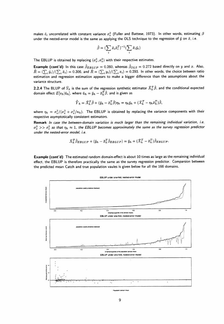
2.2.4 The BLUP of 17-h is the sum of the regression synthetic estimator .5-C9, and the conditional expected

domain effect where Uh = gh - 473, and is given as

Yh = + (gh 4)77h = rmsh + - rihgt ,

where im 0. v2/ ( 0. ;27 + ovnh \) The EBLUP is obtained by replacing the variance components with their

respective asymptotically consistent estimators.

Remark In case the between-domain variation is much larger than the remaining individual variation, i.e.0-2 >> al so that nh ti 1, the EBLUP becomes approximately the same as the survey regression predictorunder the nested-error model, i.e.

'EBLUP (gh — ±-Th EBLUP) = gh+(XT

4:)4EBLUP-

Example (cont'd) The estimated random domain-effect is about 10 times as large as the remaining individual

effect, the EBLUP is therefore practically the same as the survey regression predictor. Comparsion between

the predicted mean Catch and true population vaules is given below for all the 166 domains.

EBLUP under one-fold, nested-error model

population (solid) prediction (dashed)

..... ......... . ......

..........

0.8

1.00.0 0.2 0.4 0.6

Empirical quantile of the domain means



f. A

0. 0

0.2

0.4 0.6

0.8

1.0

Empirical gumtile ot the population domain mean


Population domain mean

a

9

Remark In the predictive approach the EBLUP is only applied to the rest population outside of the sample.

3 Generalized regression model with LINearized AREa-effect (LINARE) postulates a linear structureof the area-/domain-effect. Inference is based on the faimiliar generalized regression techinuques.Remark The random domain-effect of both the random effect and the nested-error model is trivial and cannot be 'predicted', unless the relevant domain is represented in the sample. This causes often problems inunanticipated, or badly planned, production of small area statistics — "In general the approach involvingcomponents of variance has arisen from the need to take account of the between-small-area components ofvariance. However a much more rewarding approach is to seek to explain why small areas differ." (Holt andMoura, 1993).

3.1 Consider the case with univariate auxiliary variable. The regression model which fully takes account of

the between-domain effect would allow the parameter to differ from one domain to another, i.e. for i E Uh,

yi xi/3h + ei .E[ei] = 0 and Var(e i ) = v(xi)02 .

The LINARE postulates a linear structure of 13 = (th, i3H)T through a constant (design) structure-matrixBH", and correspondingly a parameter vector of p components, such that

,3 = B.

The univariate within-domain regression model is thus replaced by a synthetic multiple regression with linearized

domain-effect. (Obviously setting B to be the H x H identity matrix recovers the complete model.) Inparticular, the structure-matrix B can arise from dummy-indexing in the same way calibration arises frompost-stratification.

Remark Given the corresponding structure matrices, the LINARE can be extended to include domain-dependent intercepts, as well as multivariate auxiliary variables, while the linear predictor remains additive.

Illustration Suppose that the domains arise from post-stratification according to Sex and Age with, say, 3age-groups. Suppose calibration w.r.t. marginal totals of both variables. The dummy indices for the post-stratification, denoted by I, and the calibration, denoted by B, and the linearization of the domian effect,involving /3 = (01, --,136) T and = (6, ..., 5 ) 7', can be expressed as

I=

/1 o 0 0 0 o\0 1 0 0 0 00 0 1 0 0 00 0 0 1 0 00 0 0 0 1 00 0 0 0 0 1

and B =

/1 o 1 o o\1 0 0 1 01 0 0 0 10 1 1 0 00 1 0 1 0

\ 0 1 0 0 1

and = f3 = Be.

3.2 Let Q = (qij ) be the n x p (sample) structure-matrix, defined according to the design structure matrix,where the i-th row corresponds to i E s. Let Qz be such that its (i, j)-th element is given by xiq ii . The

sample can thus be rewritten as

y = y = yn)T and e =

Standardize the data so that y i = yi/ViTi, and x i = xi/037, and define "O x based on x similiarly to Qz on x.Generalized regression (GREG) of y on x is the same as the OLS regression of y on i.e.

= (C2IC2x) -1 (C25) = (QTV —1 Q x) -1 (QTV'y) and diag(V) =

Typically the variance inflating constant vi takes the form vi = for some fixed r. The standardized -6 has

constant variance a 2 , whose method of mements estimator is thus given as

6'r2 = 'è") I In — rank(C2 x )}.

10

Remark The sample structure-matrix Q is usually not of the full rank, in which case deletion of the redundantcolumns are necessary.

3.3 If normality of e holds, the scaled log-likelihood and its derivatives are given as, let 7 = o2 and e ET 6. ,

21 = —n log T — el7

avia=201.617- a207= —n17 + e/72

a2 1 /ae = 0.)/T a221/a72 n/72 — 2e/7-3 .

Since ae/ae E 0 whenever evaluated at = 4, the variances of and T can be estimated separately, i.e.

liar (4) =(QT x) -11"

Var('r) = 2i-2 /{n 2rank(C2x )}.

3.4 More important, however, is the estimation of the MSE of 17h. Under the model, the BLUP is unbiased.Let 0 = (,o-2 ) and ignoring the sampling fraction, we have

E[Yh 1O] = XhBh, and Var(kh1O) = 5-2(E = 6 2 VZ,iE Uh

where Bh is the h-th row of the design structure-matrix which corresponds to domain h, i.e.

V ar(i>i,) = cr 2 11 + (XhBh)Var()(XhBh) T

Remark These variance estimates, as well as those derived under any other model, depends on the validityof the model, and should be treated with caution. For instance, it is probably unwise to base the choice ofpredictor on variances derived under their respective models alone. In fact one of the greatest challanges insmall area estimation is to develop robust and sensible measures of error and uncertainty.

Example (cont'd) In applying the LINARE to the present data, we first compared the choice of the varianceinflating constant r.

BLUP under LINARE (r=0) of domain-effect, without intercept


0.0

0.2 0.4 0.6

0.8

1.0

Empirical quanta. of the population domain mean

BLUP under LINARE (r,0.5) of domain-effect, without intercept

population (solid) predict. (dashed)

0.0

0.2

0.4

0.6

0.8

1.0

Empirical qua.. of the poputabon dom. mean



0.0

0.2

0.4 0.6

0.8

1.0

Empirical wangle of the population domain moan

11


••


•

Next we investigated whether intercept, in constant or linearized form, is necessary.

BLUP under LINARE (r=1) of domain-effect, with linearized intercept


0.0

0.2 0.4 0.6

0.8

1.0

Empirical quartile of the population domain mean

BLUP under LINARE (r=1) of domain-effect, with constant intercept

0.0

0.2 0.4 0.6

0.8

1.0



43

2

24

0.0

0:2

0.4 0.6

0.8 1.0


Fixing the LINARE at r = 1, we compare it with the nested-error model, first, for all the 109 domains whichwere represented in the sample - also shown is the direct within-domain ratio predictor.

Direct within-domain ratio predictor


2

domains which are represented in the sample

0.0

0.2

0.4 0.6

0.8

1.0



population (sad) prediction (dashed)


33

0.0

0.2

0.4 0.6

1.0

Empirical quarttile of the population domain mean


popi.dation (solid) prediction (dashed)

2


24

0.0

0.2

0.4 0.6

0.8

1.0


12

population (solid) prediction (dashed)domains which are NOT represented in the sample

.---*** ........... • • •

. .. . . ..... ... . . .... . ...... .. . ........................................

C

EC

-Ft-s

0-c)

a)0CaEC

CCa

EC

0

a)0CaEC

Cas

EC

E0

-a-0a)0

2

Ca)E

CaE00

a)0as2

We next compare the two methods for the 57 domians which were not represented in the sample.



0.0 0.2 0.4 0.6

0.8

1.0



0.0 0.2 0.4 0.6

0.8

1.0




0.0

0.2

0.4

0.6

0.8

1.0

Empirical quantile of the population domain mean



0.0 0.2 0.4 0.6

0.8

1.0

Empirical quantile of the population domain mean

The conclusion seems clear: both the LINARE and the nested-error models account adequately for the between-domain variation for the domains which were represented in the sample; however the nested-error model is

13

:42

O

O

unsuitable for those which were not represented in the sample, as compared to the LINARE.

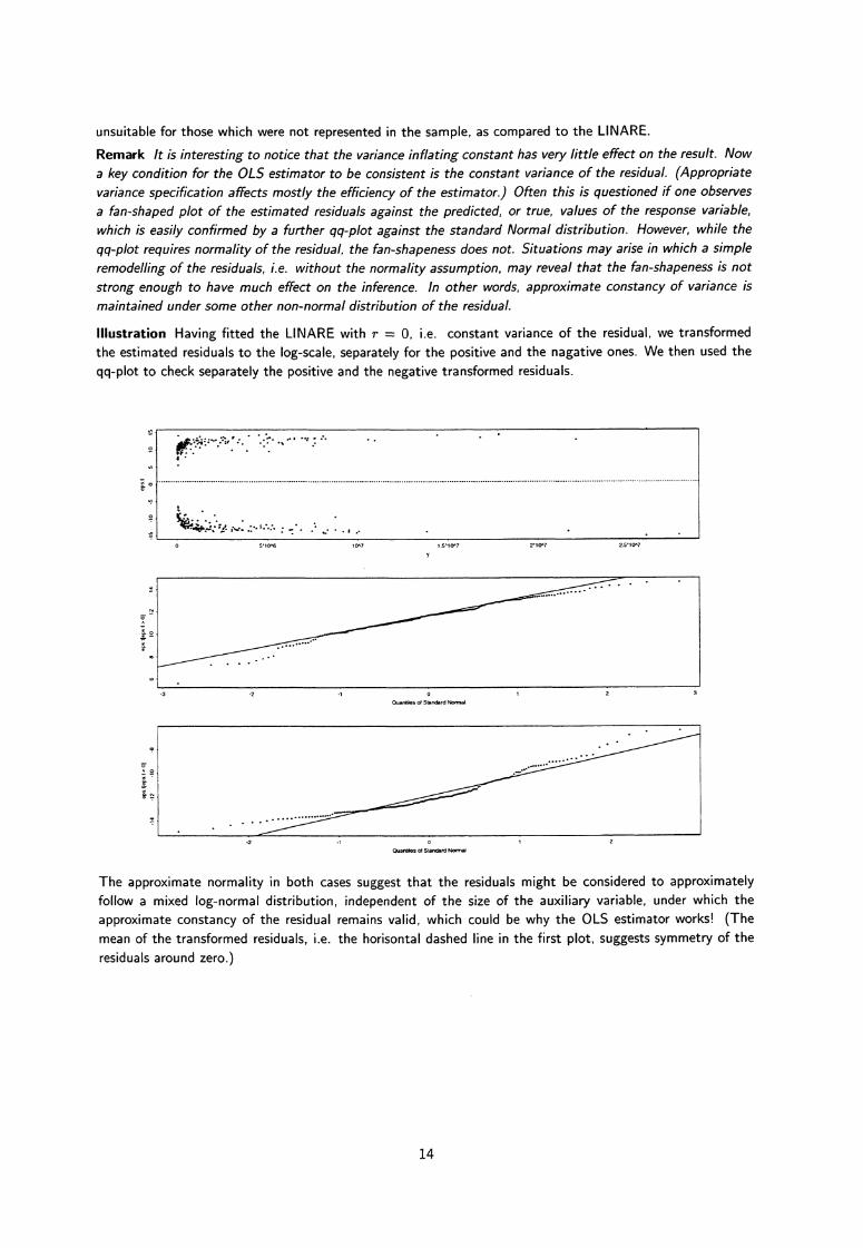
Remark It is interesting to notice that the variance inflating constant has very little effect on the result. Nowa key condition for the OLS estimator to be consistent is the constant variance of the residual. (Appropriatevariance specification affects mostly the efficiency of the estimator.) Often this is questioned if one observesa fan-shaped plot of the estimated residuals against the predicted, or true, values of the response variable,which is easily confirmed by a further qq-plot against the standard Normal distribution. However, while theqq-plot requires normality of the residual, the fan-shapeness does not. Situations may arise in which a simpleremodelling of the residuals, i.e. without the normality assumption, may reveal that the fan-shapeness is notstrong enough to have much effect on the inference. In other words, approximate constancy of variance ismaintained under some other non-normal distribution of the residual.

Illustration Having fitted the LINARE with r = 0, i.e. constant variance of the residual, we transformedthe estimated residuals to the log-scale, separately for the positive and the nagative ones. We then used theqq-plot to check separately the positive and the negative transformed residuals.

514; • •• •: .

5 . 10.6

10.7

1.5.10.7

2.5.10.7

...

.3

.2

Quartiles of Standard Normal

....... ......

• • • • • ............. •

-2 -1

0

Ouantiles of Standard Normal

The approximate normality in both cases suggest that the residuals might be considered to approximatelyfollow a mixed log-normal distribution, independent of the size of the auxiliary variable, under which theapproximate constancy of the residual remains valid, which could be why the OLS estimator works! (Themean of the transformed residuals, i.e. the horisontal dashed line in the first plot, suggests symmetry of theresiduals around zero.)

14

SMAREST (III): Models for binary survey variables

1 Apply post-stratification to the Labour Force Survey (LFS) based on auxiliary information of (i)Register-Status, (ii) Sex and (iii) Age. Let the LFS-Employment within each municipality be theinterest of the survey.

1.1 Let h, where 1 < h < H, be the post-stratum index. Let a, where 1 < a < A, be the municipality index.

Let Yah be the total LFS-Employment within munipicality a and post-stratum h. Let Pah = Yah/Nah be the

corresponding LFS-Employment Rate, where Nah is the corresponding sub-population total. Similarly, let yah

be the observed LFS-Employment in the corresponding sub-sample. Let ijah Yahinah provided nah > 0 and

Yah = 0 otherwise, where n ah is the size of the sub-sample.

1.2 The complete group-mean model allows {paid, i.e. A x H of them, to be entirely free, i.e.

Pah = Ph + ea where ph 7-= (E NahPah)/ (E Nah)-

(1)a a

2 While the synthetic estimator assumes that the post-stratum mean has null variation across themunicipalities, empirical Bayes (EB) and generalized linear mixed models (GLMM) allow for randomarea-effects. Whereas EB leads towards a constrained approach (Spjavoll and Thomsen, 1987),estimation under the GLMM is based on the penalized quasi-likelihood (Green, 1987).

2.1 The synthetic, or post-stratified, estimator can be based on the following synthetic model, i.e.

Pah = Ph ea = O. (2)

Illustration Observed within-post-stratum LFS-Employment Rate yh = (E a nahvah)I(E h)a na_, •

LFS Employment for (Register_Employment, Man)

Overall mean

E

Lij)LL N

OO

2

4 6

8

10

12

Age group

LFS Employment for (Register_Employment, Woman)

Overall mean

2

4 6

8

10

12

Age group

LFS Employment for (Register_Unemployment, Man)

•Overall mean

2

4 6

10

12

Age group

LFS Employment for (Register_Unemployment, Woman)

Overall mean

2

4

6

10

12

Age group

—cam o

I r,

.O

O

-

O

OO

15

• • • • • • • • • • • • • • • • • • • • • • •• •• • •••■•••• ••••••• •■••••.... .•

• • • • •

O °

O

overall mean 0.968

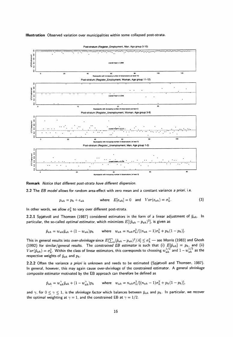
Illustration Observed variation over municipalities within some collapsed post-strata.

Post-stratum (Register_Employment, Man, Age group 3-10)

0

20

40 60 80

100

120

Municipality with increasing number of observations (at least 10)

Post-stratum (Register Employment, Woman, Age group 11-12)

°

L2-., cc.),

overall mean = 0.546

0

10 20

30


Post-stratum (Register Unemployment, Woman, Age group 3-9)

• • • • • • • • • overall mean, 0.315 . • • • • • • • •

• • . . • • • • • • • •

0

20 40 60

80

100


Post-stratum (Register Unemployment, Man, Age group 1-2)

• . •

overall mean s 0.338 • • • • •• • • • • •

0

20

40

60

80


Remark Notice that different post-strata have different dispersion.

2.2 The EB model allows for random area-effect with zero mean and a constant variance a priori, i.e.

Pah = Ph eah where E[e ah] = 0 and Var(eah) =

(3)

In other words, we allow al to vary over different post-strata.

2.2.1 Spjotvoll and Thomsen (1987) considered estimators in the form of a linear adjustment of V ah. In

particular, the so-called optimal estimator, which minimizes E[(Pah — pah ) 2 ], is given as

Pah Wahgah + (1 Wah)Ph where wah = naha2h1Rnah — 1)0i +ph(1 - ph)].

This in general results into over-shrinkage since E[E a (Pah —Pah)'/24] < — see Morris (1983) and Ghosh

(1992) for similar/general results. The constrained EB estimator is such that (i) E [pah ]

V ar(Pah) = zu Ia'I,

aWithin the class of linear estimators, this corresponds to choosing

;7_ Pwh /ii2aa nd the

i i

respective weights of gah and ph.

2.2.2 Often the variance a priori is unknown and needs to be estimated (Spjotvoll and Thomsen, 1987).

In general, however, this may again cause over-shrinkage of the constrained estimator. A general shrinkagecomposite estimator motivated by the EB approach can therefore be defined as

Pah = Wa-Y hgah + ( 1 — W -Yah)Ph where Wah -7= nahah2 IRnah 1)01„ ph(1 — ph )},

and 7 , for 0 < 7 < 1, is the shrinkage factor which balances between y ah and ph. In particular, we recover

the optimal weighting at = 1, and the constrained EB at 'y = 1/2.

16

..........................................

•..... ...............

Observed (solid) EB (dotted. sannkage_tactor = 0.1)

/ E a nah

711h — elh

71Ah eAh I

/ E a vah Vlh V2h

Vlh 1 + Vih 0and j =

0

VAh 0 • • •

VAh

0

0

1 + vAh /

• • •

u=

Illustration Over-shrinkage of the skrinkage composite estimator under the EB approach.

Post-stratum (Register_Employment, Man, Age group 3-9)

Observed (solid) EB (dolled. skrinkage_lactor . 1)

70 MATCHED municipalities (at least 10 can)

Post-stratum (Register Employment, Man, Age group 3-9)

12,ti O

O

Observed (solid) EB (dotted. sktinkage_tactor 0.5)

70 MATCHED municipalities (al least 10 obs)


70 MATCHED municipalities (at least 10 obs)

Remark It is quite clear that the constrained EB, with shrinkage factor 7 = 0.5, did not successfully adjust forover-shrinkage. We believe that this is because o was estimated based on the sample. Further investigationshould therefore consider using known variance oh a priori, for instance, based on earlier Census results.

2.3 Generalized linear mixed models (GLMM) (Breslow and Clayton, 1993) are useful for accommodating

overdispersion in binomial data — a general discussion of hierarchical generalized linear model can be found

in Lee and Nelder (1996). Under the present setting, we have

logit pah = log pah — log(1 — Pah) = eh + eah where Eleah] = 0 and V ar(eah) = (4)

2.3.1 Without restrictions on eah, the maximum likelihood estimator (mle) results into over-fitting. A penalized

(quasi) log-likelihood (Green, 1987) can be defined here as

le(h,011,;Y) =[EYah(eh e ah)±71ahlOg(1 Pah)i — eah,

a a

where the last term on the right-hand side is the penalty to be paid for non-zero random effects.

2.3.2 Estimation based on 1 e employs Fisher

andFor the present values of and eah,nd v

according to (4), and let rah Yah — nahPah = nahPah( 1— Pah), and

calculate pa h

g°.21„2

,1)O

Update 9 = elh, eAh) T as 0 + j — lu, and iterate till convergence, upon which estimate based on

the estimated eah.

17

....................... ......................

Observed (solid) GLMM (dotted)

.................................................

Observed (solid) GLMM (dotted)

.........

................................

Observed (wild) GLMM (dotted)

12

2ea .

Illustration Fitting GLMM to some collapsed post-strata.



Post-stratum (Register Employment, Woman, Age group 11-12)


Post-stratum (Register Unemployment, Woman, Age group 3-9)

..... ....................................Observed (solid) GLMM (dotted)

................


Post-stratum (Register Unemployment, Man, Age group 1-2)


3 The random area-effect model of the GLMM-type can be defined at the level of municipality. Alinear structure can be introduced to accommodate area-specific post-stratification, which allows forbetter data usage. A similar linear structure can be introduced for the random area-effect to accountfor difference between the sample and population configurations.

3.1 Let pa be the LFS-Employment Rate of municipality a, with auxiliary vector X a which, typically, arises

from calibrating post-stratification (Zhang, 1998). Based on the sample, we define, for t' a = xa/na,

logit pa = xa ± ea where E[ea] = 0 and Var(e a )

(5)

In this way, within each municipality, there is only one random effect. Notice that, the usual GLM is obtained

from setting ea E 0. Estimation is, as under(4), based on the penalized quasi log-likelihood, defined as

(72 ; Y) = [E Ya (±7a' + e a ) + na log(1 — pa)] —a a

Let na = Ya naPa and va = napa (1 —pa ). Let e = (e i ,..., eA) T , and 77 = , and V the diagonal

matrix with va as the ath element on the diagonal. Let B = (baj) be the A x q design matrix whose ath row

is given by -±a , and

g

t!

1°!;

„,

OO

OO

BT 77 = 77

—e andB . TVB BTV

3 VB I +V

where I is the A x A identity matrix. Update 0 = eq, et , ..., eA) T as 8 + j'u, and iterate till

convergence, upon which estimate cr2 based on the estimated ea .

18

...............................

............................... • .................

Observed (sdid) GLM (dotted)

..............

.......................................

Observed (solid) GLOM (dotted)

................. •

Observed (solid) Adjusted Register (dotted)

Illustration Fitting GLM and GLMM with random area-effect to random sub-sample of the LFS (I).

LFS-Employment Rate within 108 UNMATCHED municipalities

Municipality (at least 5 obs)


Municipality (at bast 5 obs)


Muniapality (at least 5 obs)

Illustration Fitting GLM and GLMM with random area-effect to random sub-sample of the LFS (II).

LFS-Employment Rate within 76 MATCHED municipalities

tr, °

ut.)Observed (solid) GLM (dotted)

7E

Cu- ;

°

;

72,



• • „

Observed (sohd) GLMM (dotted)



••

Observed (solid) Adjusted Register (dotted)

;


19

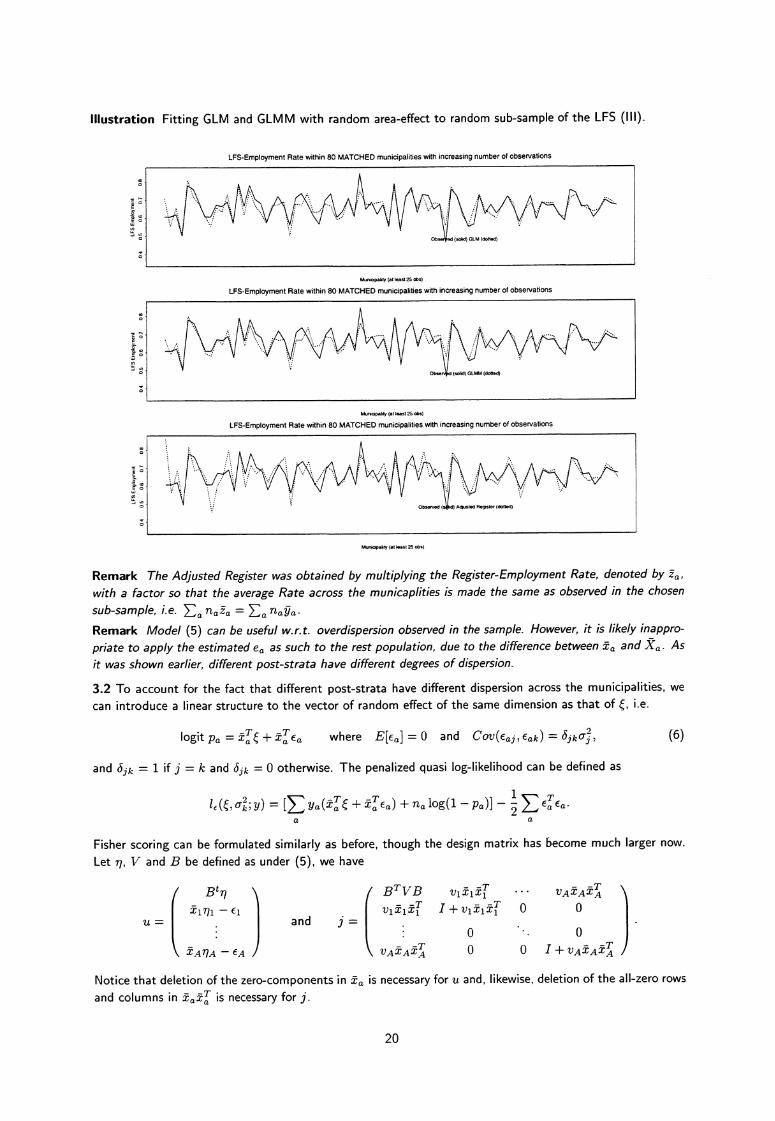
Illustration Fitting GLM and GLMM with random area-effect to random sub-sample of the LFS (Ill).

LFS-Employment Rate within 80 MATCHED municipalities with increasing number of observations

(solid) GLM (dotted)

Munsopabty (at least 25 obs)


(solid) GLMM (dotted)

Munsopabty (at least 25 obs)


Observed

Id) Adjusted Register (dotted)

Municipality (at Was' 25 obs)

Remark The Adjusted Register was obtained by multiplying the Register-Employment Rate, denoted by za ,with a factor so that the average Rate across the municaplities is made the same as observed in the chosensub-sample, i.e. E a na fa => a nag..Remark Model (5) can be useful w.r.t. overdispersion observed in the sample. However, it is likely inappro-priate to apply the estimated ea as such to the rest population, due to the difference between ".±a, and fCa . Asit was shown earlier, different post-strata have different degrees of dispersion.

3.2 To account for the fact that different post-strata have different dispersion across the municipalities, wecan introduce a linear structure to the vector of random effect of the same dimension as that of i.e.

logit pa, ga ea where Ejfai = 0 and COV(Eaj, Eak) Ojkaj,

(6)

and Oik = 1 if j = k and Sik = 0 otherwise. The penalized quasi log-likelihood can be defined as

1E (e7 C12; y) = [E Ya( Ta e ±1 6a) na 100 Pa)] —1 x- T

—2 1- Ea Ea.a a

Fisher scoring can be formulated similarly as before, though the design matrix has become much larger now.Let 77 , V and B be defined as under (5), we have

B t n I BTVB

-±, -±T vAt- A±5.

—

I +

f,LL

7,

u= and j =. 0 0

vAxAxA 0 0 I + vAXAtTA )471A — EA I

Notice that deletion of the zero-components in -±a is necessary for u and, likewise, deletion of the all-zero rowsand columns in -± a 2Ta is necessary for j.

20

References

Ansen, H., HaIlen, S.-A., and Ylander, H. (1988). Statistics for regional and local planning in Sweden. J. Off.Statist., 4, 35-46.

Battese, G.A., Harter, R.M., and Fuller, W.A. (1988). A error-component model for prediction of county cropareas using survey and satelite data. J. Amer. Statist. Assoc., 83, 28-36.

Brackstone, G.J. (1987). Small area data: policy issues and technical challenges. In Small Area Statistics, ed.by R. Platek, J. Rao, C.-E. S5rndal, and M. Singh, pp. 3-20. Wiley, New York.

Breslow, N.E. and Clayton, D.G. (1993). Approximate inference in generalized linear mixed models. J. Amer.Statist. Assoc., 88, 9-25.

Chambers, R.L. and Feeney, G.A. (1977). Log linear models for small area estimation. Unpublished paper,Australian Bureau of Statistics.

Chaudhuri, A. (1992). Small domain statistics: A review. Technical Report ASC/92/2, Indian StatisticalInstitute, Calcutta.

Cressie, N. (1989). Empirical Bayes estimation of undercount in the decennial census. J. Amer. Statist. Assoc.,84, 1033-44.

Cressie, N. (1992). REML estimation in empirical Bayes smoothing of census undercount. Survey Methodology,18, 75-94.

Datta, G.S: and Ghosh, M. (1991). Bayesian prediction in linear models: Applications to small area estimation.Ann. Statist., 19, 1748-70.

Decaudin, G. and Labat, J.-C. (1997). A synthetic, robust and efficient method of making small area popula-tion estimates in France. Survey Methodology, 23, 91-8.

DeSouza, C.M. (1992). An approximate bivariate Bayesian method for analyzing small frequencies. Biometrics,48, 1113-30.

Drew, D., Singh, M.P., and Choudhry, G.H. (1982). Evaluation of small area estimation techniques for theCanadian Labour Force Survey. Survey Methodology, 8, 17-47.

Ericksen, E.P. (1974). A regression method for estimating populations of local areas. J. Amer. Statist. Assoc.,69, 867-75.

Ericksen, E.P. and Kadane, J.B. (1985). Estimating the population in a census year (with discussion). J. Amer.Statist. Assoc., 80, 98-131.

Ericksen, E.P. and Kadane, J.B. (1987). Sensitivity analysis of local estimates of undercount in the 1980 U.S.Census. In Small Area Statistics, ed. by R. Platek, J. Rao, C.-E. S5rndal, and M. Singh, pp. 23-45. Wiley,New York.

Ericksen, E.P., Kadane, J.B., and Tukey, J.W. (1989). Adjusting the 1981 census of population and housing.J. Amer. Statist. Assoc., 84, 927-44.

Falorsi, P.D., Falorsi, S., and Russo, A. (1994). Empirical comparison of small area estimation methods forthe Italian Labour Force Survey. Survey Methodology, 20, 171-76.

Fay, R.E. and Herriot, R.A. (1979). Estimates of income for small places: an application of James-Stein pro-cedures to census data. J. Amer. Statist. Assoc., 74, 269-77.

Freedman, D.A. and Navidi, W.C. (1986). Regression models for adjusting the 1980 Census (with discussion).Statistical Science, 1, 1-39.

Freedman, D.A. and Navidi, W.C. (1992). Should we have adjusted the U.S. Census of 1980? (with discus-sion). Survey Methodology, 18, 3-74.

Freeman, D.H. and Koch, G.G. (1976). An asymptotic covariance structure for testing hypotheses on rakedcontingency tables from complex sample surveys. In Proccedings of the Social Statistics Section, pp. 330-5.

Amer. Statist. Assoc., Washington, DC.

Fuller, W.A. and Battese, G.E. (1973). Transformations for estimation of linear models with nested-error struc-ture. J. Amer. Statist. Assoc., 68, 626-32.

Fuller, W.A. and Harter, R.M. (1987). The multivariate components of variance model for small area estima-tion. In Small Area Statistics, ed. by R. Platek, J. Rao, C.-E. Sarndal, and M. Singh, pp. 103-23. Wiley,

New York.

Ghosh, M. (1992). Constrained Bayes estimation with applications. J. Amer. Statist. Assoc., 87, 533-40.

Ghosh, M. and Larihi, P. (1987). Robust empirical Bayes estimation of means from stratified samples. J. Amer.Statist. Assoc., 82, 1153-62.

Ghosh, M., Natarajan, K., Stroud, T.W.F., and Carlin, B.P. (1998). Generalized linear models for small-areaestimation. J. Amer. Statist. Assoc., 93, 273-82.

Ghosh, M. and Rao, J.N.K. (1994). Small area estimation: An appraisal (with discussion). Statistical Science,9, 55-93.

Gonzalez, M.E. (1973). Use and evaluation of synthetic estimators. In Proceedings of the Social StatisticsSection, pp. 33-6. Amer. Statist. Assoc., Washington, DC.

Green, P.J. (1987). Penalized likelihood for general semi-parametric regression models. Int. Statist. Rev., 55,245-59.

Harville, D.A. (1977). Maximum likelihood approaches to Variance Component estimation and to relatedproblems. J. Amer. Statist. Assoc., 72, 320-38.

Heldal, J., Swensen, A.R., and Thomsen, I. (1987). Census statistics through combined use of surveys andregisters. Statistical Journal of the United Nations ECE, 5, 43-51.

Holt, D. and Moura, F. (1993). Mixed models for making small area estimates. In Small Area Statistics andSurvey Designs, ed. by G. Kalton, J. Kordos, and R. Platek, vol. 1, pp. 221-31. Central Statistical Office,

Warsaw.

Holt, D. and Smith, T.M.F. (1979). Post stratification. J. Roy. Statist. Soc. A, 142, 33-46.

Isaki, C.T., Schultz, L.K., Smith, P.J., and Diffendal, D.J. (1987). Small area etimation research for censusundercount - progress report. In Small Area Statistics, ed. by R. Platek, J. Rao, C.-E. S5rndal, and M. Singh,

pp. 219-38. Wiley, New York.

Kalton, G., Kordos, J., and Platek, R. (1993). Small Area Statistics and Survey Designs Vol 1: Invited Papers;Vol II: Contributed Papers and Panel Discussion. Central Statisticcal Office, Warsaw.

Kass, R.E. and Steffey, D. (1989). Approximate Bayesian inference in conditionally independent hierarchicalmodles (parametric empirical Bayes models). J. Amer. Statist. Assoc., 84, 717-26.

Laake, P. (1978). An evaluation of synthetic estimates of employment. Scand. J. Statist, 5, 57-60.

Laake, P. (1979). A predictive approach to subdomain estimation in finite populations. J. Amer. Statist. Assoc.,74, 355-8.

Laird, N.M. and Louis, T.A. (1987). Empirical Bayes confidence intervals based on bootstrap samples. J.Amer. Statist. Assoc., 82, 739-50.

Lee, Y. and Nelder, J.A. (1996). Hierarchical generalized linear models (with discussion). J. Roy. Statist. Soc.B, 58, 619-78.

Louis, T. (1984). Estimating a population of parameter values using bayes and empirical Bayes methods. J.Amer. Statist. Assoc., 79, 393-8.

Lui, K.-J. and Cumberland, W.G. (1991). A model-based approach: composite estimators for small area esti-mation. J. Off. Statist., 7, 69-76.

Lundstrom, S. (1987). An evaluation of small area estimation methods: The case of estimating the number ofnonmarried cohabiting persons in Swedish munucipalities. In Small Area Statistics, ed. by R. Platek, J. Rao,C.-E. Sarndal, and M. Singh, pp. 239-56. Wiley, New York.

Marker, D.A. (1983). Organization of small area estimators. In Proceedings of Survey Research MethodsSection, pp. 409-14. Amer. Statist. Assoc., Washington, DC.

Morris, C. (1983). Parametric empirical Bayes inference: Theory and applications (with discussion). J. Amer.Statist. Assoc., 78, 47-65.

Morrison, P. (1971). Demographic information for cities: a manual for estimating and projecting local popu-lation characteristics. RAND report R-618-HUD.

Nordbotten, S. (1996). Neural Network imputation applied to the Norwegian 1990 population census data. J.Off. Statist., 12, 385-401.

Platek, R., Rao, J.N.K., S5rndal, C.-E., and Singh, M.P. (1987). Small Area Statistics. Wiley, New York.

Platek, R. and Singh, M.P. (1986). Small Area Statistics: Contributed Papers. Laboratory for Research inStatistics and Probability, Carleten Univ.

Prasad, N.G. and Rao, J.N.K. (1990). The estimation of mean square errors of small area estimators. J. Amer.Statist. Assoc., 85, 163-71.

Purcell, N.J. (1979). Efficient Small Domain Estimation: A categorical data analysis approach. Ph.D. thesis,Univ. of Michigan, Ann Arbor, Michigan.

Purcell, N.J. and Kish, L. (1979). Estimation for small domain. Biometrics, 35, 365-84.

Purcell, N.J. and Kish, L. (1980). Postcensal estimates for local areas (or domains). Int. Statist. Rev., 48,3-18

Raghunathan, T.E. (1993). A quasi-empirical Bayes method for small area estimation. J. Amer. Statist. Assoc.,88, 1444-8.

Rao, J.N.K (1986). Synthetic estimators, SPREE and best model based predictors. In Proceedings of theConference on Survey Research Methods in Agriculture, pp. 1-16. U.S. Dept. Agriculture, Washington, DC.

Robinson, G.K. (1991). That BLUP is a good thing: the estimation of random effects (with discussion).Statistical Science, 6, 15-51.

Sarndal, C.-E. and Hidiroglou, M.A. (1989). Small domain estimation: a conditional analysis. J. Amer. Statist.Assoc. , 84, 266-75.

Schaible, W.L. (1978). Choosing weights for composite estimators for small area statistics. In Proceedings ofSurvey Research Methods Section, pp. 741-6. Amer. Statst. Assoc., Washington DC.

Singh, M.P., Gambino, J., and Mantel, H. (1993). Issues and options in the provision of small area data. InSmall Area Statistics and Survey Designs, ed. by G. Kalton, J. Kordos, and R. Platek, vol. 1, pp. 37-75.

Central Statistical Office, Warsaw.

Small Area Estimation Research Team (1983). A bibliography for small area estimation. Survey Methodology,9, 241-61.

Spjavoll, E. and Thomsen, I. (1987). Application of some empirical Bayes methods to small area statistics.Bulletin of the International Statistical Institute, 2, 435-49.

Statistics Canada (1987). Population Estimation Methods, Canada. Catalogue 91-528E. Statistics Canada,

Ottawa.

Stukel, D. (1991). Small Area Estimation Under One and Two-fold Nested Error Regression Model. Ph.D.

thesis, Carleton Univ.

Zhang, L.-C. (1998). Post-stratification and calibration — A synthesis. Statistics Norway (Discussion paperNo. 216).

Zidek, J.V. (1982). A review of methods for estimating the populations of local areas. Technical Report 82-4,Univ. British Columbia, Vancouver.

Recent publications in the series Documents

97/9 H. Berby and Y. Bergstrom: Development of aDemonstration Data Base for Business RegisterManagement. An Example of a StatisticalBusiness Register According to the Regulationand Recommendations of the European Union

97/10 E. Holmoy: Is there Something Rotten in thisState of Benchmark? A Note on the Ability ofNumerical Models to Capture Welfare Effects dueto Existing Tax Wedges

97/11 S. Blom: Residential Consentration amongImmigrants in Oslo

97/12 0. Hagen and H.K. Ostereng: Inter-BalticWorking Group Meeting in Bodo 3-6 August1997 Foreign Trade Statistics

97/13 B. Bye and E. Holmoy: Household Behaviour inthe MSG-6 Model

97/14 E. Berg, E. Canon and Y. Smeers: ModellingStrategic Investment in the European Natural GasMarket

97/15 A. Braten: Data Editing with Artificial NeuralNetworks

98/1 A. Laihonen, I. Thomsen, E. Vassenden andB. Laberg: Final Report from the DevelopmentProject in the EEA: Reducing Costs of Censusesthrough use of Administrative Registers

98/2 F. Brunvoll: A Review of the Report"Environment Statistics in China"

98/3: S. Holtskog: Residential Consumption ofBioenergy in China. A Literature Study

98/4 B.K. Wold: Supply Response in a Gender-Perspective, The Case of Structural Adjustmentsin Zambia. Tecnical Appendices

98/5 J. Epland: Towards a register-based incomestatistics. The construction of the NorwegianIncome Register

98/6 R. Chodhury: The Selection Model of SaudiArabia. Revised Version 1998

98/7 A.B. Dahle, J. Thomasen and H.K. Ostereng(eds.): The Mirror Statistics Exercise between theNordic Countries 1995

98/8 H. Berby: A Demonstration Data Base forBusiness Register Management. A data basecovering Statistical Units according to theRegulation of the European Union and Units ofAdministrative Registers

98/9 R. Kjeldstad: Single Parents in the NorwegianLabour Market. A changing Scene?

98/10 H. Briingger and S. Longva: InternationalPrinciples Governing Official Statistics at theNational Level: are they Relevant for theStatistical Work of International Organisations aswell?

98/11 H.V. Smbo and S. Longva: Guidelines forStatistical Metadata on the Internet

98/12 M. Ronsen: Fertility and Public Policies -Evidence from Norway and Finland

98/13 A. BrAten and T. L. Andersen: The ConsumerPrice Index of Mozambique. An analysis ofcurrent methodology — proposals for a new one. Ashort-term mission 16 April - 7 May 1998

98/14 S. Holtskog: Energy Use and Emmissions to Airin China: A Comparative Literature Study

98/15 J.K. Dagsvik: Probabilistic Models for QualitativeChoice Behavior: An introduction

98/16 H.M. Edvardsen: Norwegian Regional Accounts1993: Results and methods

98/17 S. Glomsrod: Integrated Environmental-EconomicModel of China: A paper for initial discussion

98/18 H.V. Smbo and L. Rogstad: Dissemination ofStatistics on Maps

98/19 N. Keilman and P.D. Quang: Predictive Intervalsfor Age-Specific Fertility

98/20 K.A. Brake (Coauthor on appendix: Jon Gjerde):Hicksian Income from Stochastic Resource Rents

98/21 K.A.Brekke and Jon Gjerde: OptimalEnvironmental Preservation with StochasticEnvironmental Benefits and IrreversibleExtraction

99/1 E. Holm0y, B. Strom and T. Avitsland: Empiricalcharacteristics of a static version of the MSG-6model

99/2 K. Rypdal and B. Toms* Testing the NOSEManual for Industrial Discharges to Water inNorway

99/3 K. Rypdal: Nomenclature for Solvent Productionand Use

99/4 K. Rypdal and B. Toms* Construction ofEnvironmental Pressure Information System(EPIS) for the Norwegian Offshore Oil and GasProduction

99/5 M. Soberg: Experimental Economics and the USTradable SO2 Permit Scheme: A Discussion ofParallelism

99/6 J. Epland: Longitudinal non-response: Evidencefrom the Norwegian Income Panel

Returadresse:Statistisk sentralbyraPostboks 8131 Dep.N-0033 Oslo

Documents PORTO BETALTVED

INNLEVERINGAPP

VP.NORGE/NOREG

Tillatelse nr.159 000/502

Statistics NorwayP.O.B. 8131 Dep.N-0033 Oslo

Tel: +47-22 86 45 00Fax: +47-22 86 49 73

ISSN 0805-9411

00 Statistisk sentralbyrfi4110 Statistics Norway