small world networks made and presented by : harshit bhatt 901929988
TRANSCRIPT

SMALL WORLD NETWORKS
Made and Presented By :
Harshit Bhatt
901929988

WHAT ARE SMALL WORLD NETWORKS? In general a network is considered Small-World Network if the mean geodesic distance(path
length) between all pair of nodes in the network is small as compared to the total number of nodes in the network.
This can also be considered as if one could reach any other random member in the graph/network within small number of hops.(generally considered <=6)
A general formula for considering a network as Small-World is that the Path Length(L) of the network must increase in direct proportion to the logarithm of the total no of nodes(N).
(i.e. )
Examples of this type of network are Social Network, Internet, Human Genes etc.
The major redefinition on the Small-World networks was done by Duncan J. Watts and Steven Strogatz in their 1998 joint Nature Paper further which it starts to be known as Watts–Strogatz Model.
In their 1998 landmark paper, Watts and Strogatz described small-world networks as those which are “highly clustered, like regular lattices, yet have small characteristic path lengths, like random graphs”.

Since that original paper, numerous networks have been described as exhibiting small-world properties, including systems as diverse as the Internet, social groups, and biochemical pathways.
After the Watts-Strogatz paper there was a deluge of research papers on this topic.
Noted ones of them were the Newman and Watts 1999a and 1999b, Argollo de Menezes et al., 2000, Albert and Barabasi 2002, Newman 2003, Newman2010, Joyce, Telesford and Laurineti, 2011.
Newman have a great contribution in the Small World Network due to his various influential research.
He with Watts produced a variant of the WS Model to generate Small World Networks which is used as latest definition of WS Model.
Image on the left shows the general construction of Small World Network according to Watts-Strogatz Model for 20 Nodes where random edges are added to lower the network path length.
Whereas the image on the right shows a Watts-Strogatz Small world Model of 100 Nodes as generated by Cytoscape.
Where Albert and Barabasi helped to formulate the two most important aspects in the Small World Networks, Clustering Coefficient(C) and Path Length(L) which helped to define the Small World Networks in great detail and new light.

Mathematically, C is the proportion of edges ei that exist between the neighbors of a particular node (i) relative to the total number of possible edges(ki) between neighbors. Hence we could formulate it as :
After which we take the mean of all nodes Clustering Coefficient to evaluate C.
Path length is a measure of the distance between nodes in the network, calculated as the mean of the shortest geodesic distances between all possible node pairs :
where, d(vi, vj) is the shortest geodesic distance between nodes i and j n = total number of vertices in the Graph
Watts and Strogatz developed a network model (WS model) that resulted in the first-ever networks with clustering close to that of a lattice and path lengths similar to those of random networks. The WS model demonstrates that random rewiring of a small percentage of the edges in a lattice results in a precipitous decrease in the path length, but only trivial reductions in the clustering. Across this rewiring probability, there is a range where the discrepancy between clustering and path length is very large, and it is in this area that the benefits of small-world networks are realized.
(ref. : http://www.ncbi.nlm.nih.gov/pmc/articles/PMC3604768/#!po=20.8333)

In early days Small-World Networks were considered as a subset of only Random Networks but Watts and Strogatz proposed that the Small-World Networks exhibit the nature of both Regular Lattice like structure Network and Random Networks.
Where the Real World Networks(mostly small-world networks) have small Path Length(L) as in ‘Random Networks’ they also have high Clustering Coefficient(C) as seen in “large-world” Regular Networks(such as lattice).
Variants of Watts-Strogatz Model(Small World Networks)
(ref : https://cascade.madmimi.com/promotion_images/0643/1044/original/Small-world-network-.png?1395142912) (ref : http://optimizationandanalytics.files.wordpress.com/2013/01/complex-network-structure.png)

Even though WS Model made Small World independent of Random Networks the small world property was still formulated on Random Networks alone.
Humphry and his team in 2006 gave the first formula to measure the small world property but it was totally dependent on the comparison with the equivalent random network of small world model.
(given by Humphries et al., 2006)
where, σ = Small World Measurement
Lrand = Path length of the equivalent random network
Crand = Clustering Coefficient of the equivalent random network
L = Path length of the Small-World(real) Network
C = Clustering coefficient of the Small-World(real) Network
γ and λ being the ratios for clustering and path length between real and equivalent random network. The conditions that must be met for a network to be classified as small-world
are C≫Crand and L≈Lrand, which results in σ>1.
Comparing path length to that of a random network makes sense—the path length of a small-world network should be short, like that of a random network. However, the comparison of clustering to an equivalent random network does not properly capture small-world behavior because clustering in a small-world network more closely mimics that of a lattice network. Furthermore, it is generally accepted that clustering in the original network is much greater than that of a random network.

Consider two networks, A and B, with similar path lengths yet disparate clustering coefficients of 0.5 and 0.05, respectively. If the clustering coefficients of the equivalent random networks are both 0.01, then network A clearly has greater small-world properties. However, if the clustering of the random networks for A and B are 0.01 and 0.001, respectively, then the two networks will have similar values of σ. Interpretation of σ suggests that both networks have the same small-world characteristics even though network B has considerably lower clustering.
The comparison of clustering to a random network presents several limitations to the use of σ. The σ ranges from 0 to ∞ and differ even with the network size even if the clustering and path length are same.
Due to high discrepancy in measuring the small world properties by comparing it with the Random Network alone the later researchers came to a solution in which they took both highly clustered lattice-like structure and random network properties to compare to the small(real) world networks.
Later researchers came to the formula : (given by Joyce,Telesford,Laurineti, 2011)
where, ω = Small World Measurement
Lrand = Path length of the equivalent random network
Clatt = Clustering Coefficient of the equivalent lattice-like network
L = Path length of the Small-World(real) Network
C = Clustering coefficient of the Small-World(real) Network

This formula could be used for any size of structure and the best part is that it has the range of small world property from -1 to +1 which makes it easy to distinguish the Small World Networks which lie in the range around 0, also if ω is close to -1 it shows the Regular Network property while near +1 it shows the Random Network.
The network in the left shows the difference in the Small World measurement in later and earlier evaluations depending on the network size. Where in earlier(right) the value differs for different network size, in the later(left) the value is same for every network size corresponding to the different Rewiring probability.
(ref. : http://www.ncbi.nlm.nih.gov/pmc/articles/PMC3604768)
The other major benefit of the new formula is that it also helps in deciding whether a network is Random or Regular which was not possible in the earlier formula, hence it proves to be of great help while studying various Real World Networks as it helps to decide their properties.
One possible reason why comparisons with network lattices have not been used in the literature up to this point is the length of time it takes to generate lattice networks, particularly for large networks. One appeal of comparing the original network to only a random network is the rather fast processing time to generate the random network. Although latticization is fast in smaller networks, large networks such as functional brain networks and the Internet can take several hours to generate and optimize.

(ref. : http://www.ncbi.nlm.nih.gov/pmc/articles/PMC3604768)
Image to the left explains the stark contrast between small-world measurements earlier(right half) and now(left half).
The dotted line represents the small-world measurement which varies highly in the earlier method and have a low variety in the later method.
The squares represent the clustering coefficient, circles the path length and p the rewiring probability of the network.
Where in the later measurement small-world coefficient(ω) near 0 represents small world property, in earlier the coefficient(σ) above 1 represents the small world network. Hence with the earlier formula every network except when p=1 is considered a small world network whereas later only a handful networks (ω ≈ 0) can be considered small world(which is true as for real world networks).
Comparing earlier and later approaches to measure Small World Property
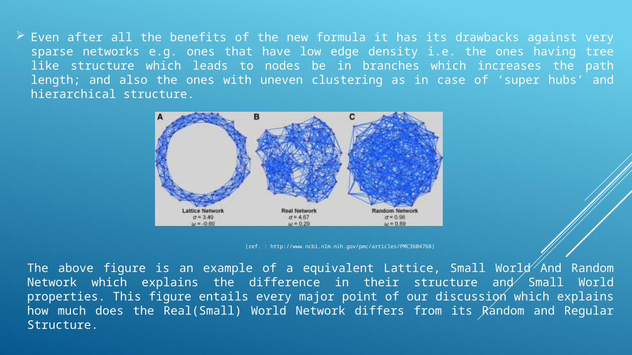
Even after all the benefits of the new formula it has its drawbacks against very sparse networks e.g. ones that have low edge density i.e. the ones having tree like structure which leads to nodes be in branches which increases the path length; and also the ones with uneven clustering as in case of ‘super hubs’ and hierarchical structure.
The above figure is an example of a equivalent Lattice, Small World And Random Network which explains the difference in their structure and Small World properties. This figure entails every major point of our discussion which explains how much does the Real(Small) World Network differs from its Random and Regular Structure.
(ref. : http://www.ncbi.nlm.nih.gov/pmc/articles/PMC3604768)

Another point to mention is that when we are comparing equivalent Random and Regular networks with the Real Network the coefficients such as Clatt and Lrand are evaluated with taking average of many such (Regular or Random) networks.
Let in our study, for constructing an equivalent Random Network we make edges rewired at random an average of 10 times for the actual network. Let this Network randomization be performed for 50 different equivalent Random Networks, with the clustering coefficient and path length calculated for each network through which we get the Crand and Lrand of the equivalent Random Network. It is important to note that ω or σ is valid only if the comparable Random Network preserves the degree distribution of the original network.
The Lattice(Regular) Network is generated by using a modified version of the “latticization” algorithm (Sporns and Zwi, 2004). The procedure is based on a Markov-chain algorithm that maintains node degree and swaps edges with uniform probability; however, swaps are carried out only if the resulting matrix has entries that are closer to the main diagonal. To optimize the clustering coefficient of the lattice network, the latticization procedure is performed over several user-defined repetitions. Storing the initial adjacency matrix and its clustering coefficient, the latticization procedure is performed on the matrix. If the clustering coefficient of the resulting matrix is lower, the initial matrix is kept and latticization is performed again on the same matrix; if the clustering coefficient is higher, then the initial adjacency matrix is replaced. This latticization process is repeated until clustering is maximized.
Constructing Equivalent Random and Regular Networks of a Real Network

The figure on the left shows (a) A ring network in which each node is connected to the same number l=3 nearest neighbors on each side. (This network resembles a one-dimensional lattice with periodic boundary conditions.) (b) A Watts-Strogatz network is created by removing each edge with uniform, independent probability p and rewiring it to yield an edge between a pair of nodes that are chosen uniformly at random. (c) The Newman-Watts variant of a Watts-Strogatz network, in which one adds "shortcut" edges between pairs of nodes in the same way as in a WS network but without removing edges from the underlying lattice.
Watts – Strogatz and Newman - Watts Networks
To discuss the Watts-Strogatz family of small-world networks, we need a notion of clustering. A global clustering coefficient is : C = (3 * Number of triangles)/ number of connected triples.
As we can see from the figure above a triangle would be constructed when a triangle consists of 3 nodes that are completely connected to each other (i.e., a 3-clique) and a connected triple consists of three nodes {i,j,k} such that node i is connected to node j and node j is connected to node k. The factor of 3 arises because each triangle gets counted 3 times in a connected triple. The clustering coefficient C indicates how many triples are in fact triangles. A complete graph, in which every pair of nodes is connected by an edge, with N≥3 nodes yields the maximum possible value of C=1, as all triples are also triangles. The minimum value of the clustering coefficient is C=0.
The WS model, which is parameterized by p(Rewiring Probability)∈[0,1], includes a regime of networks that simultaneously exhibit both significant clustering and the small-world property. When p=0, we obtain a ring graph in which each node is coupled to its c(degree)=2l nearest neighbors; when p=1, we obtain an ER random graph.
(ref. : http://www.scholarpedia.org/article/Small-world_network)

When one states a property of the WS model for a fixed set of parameter values (and with p≠0), it is to be understood as a mean over an ensemble of graphs.
As it is problematic to define WS Model for p=0, hence Newman proposed his theory which we could see in the fig. (c) part, where when adding a random edge between two nodes we need not to remove a direct edge between the node and its neighbors.
Therefore using Newman’s theory for p=0, the clustering coefficient is : C = 3(c-2)/4(c-1). This is independent of the no. of nodes and varies from C=0 for c=2 to C→3/4 for c→∞.
One can see using numerical computations that WS networks have high C and low ℓ for many values of p, but it is not easy to verify these features with rigorous calculations. In an NW network(fig. c), the substrate ring(fig. a) remains intact, which simplifies calculations enormously. The downside is that C↛0 as p→1 (for c>2), as one no longer obtains an ER random graph in that limit. Hence, the NW variant of the WS model has similar behavior for small and intermediate values of p but not for values of p that are too close to 1.
To examine the small-world property, it is desirable to have an expression for the mean geodesic distance L. In NW networks, one can show using scaling considerations and a mean-field approximation that : L ~ (N/c) * f(Ncp)
where, f(x) ~ 2/ rt(x2 + 4x) tanh-1 (rt(x/x+4))
and Ncp is the expected number of shortcut edges

Clustering coefficient C and mean geodesic distance ℓ between nodes in the Newman-Watts variant of the Watts-Strogatz small-world model as a function of rewiring probability p. Observe that there is a regime with high clustering but low mean geodesic distance. The clustering coefficient C∈[0,1], as one obtains C=1 for a complete graph with N≥3 nodes.
(ref. : http://www.scholarpedia.org/article/Small-world_network)

QUESTIONS?

THANK YOU FOR YOUR COOPERATION.
For further Queries and Information please contact me :