i

SMALL, SHORT DURATION TECHNICAL TEAM DYNAMICS

S-RES-024-XXX-R2-04

PAMELA JO KNIGHT, PH.D.

FINAL RESEARCH REPORT

MAY 2006

PUBLISHED BY THE DEFENSE ACQUISITION UNIVERSITY PRESS FORT BELVOIR, VIRGINIA

Report Documentation Page Form ApprovedOMB No. 0704-0188

Public reporting burden for the collection of information is estimated to average 1 hour per response, including the time for reviewing instructions, searching existing data sources, gathering andmaintaining the data needed, and completing and reviewing the collection of information. Send comments regarding this burden estimate or any other aspect of this collection of information,including suggestions for reducing this burden, to Washington Headquarters Services, Directorate for Information Operations and Reports, 1215 Jefferson Davis Highway, Suite 1204, ArlingtonVA 22202-4302. Respondents should be aware that notwithstanding any other provision of law, no person shall be subject to a penalty for failing to comply with a collection of information if itdoes not display a currently valid OMB control number.

1. REPORT DATE MAY 2006

2. REPORT TYPE N/A

3. DATES COVERED -

4. TITLE AND SUBTITLE Small, Short Duration Technical Team Dynamics

5a. CONTRACT NUMBER

5b. GRANT NUMBER

5c. PROGRAM ELEMENT NUMBER

6. AUTHOR(S) 5d. PROJECT NUMBER

5e. TASK NUMBER

5f. WORK UNIT NUMBER

7. PERFORMING ORGANIZATION NAME(S) AND ADDRESS(ES) The Defense Acquisition University Press Fort Belvoir, VA

8. PERFORMING ORGANIZATIONREPORT NUMBER

9. SPONSORING/MONITORING AGENCY NAME(S) AND ADDRESS(ES) 10. SPONSOR/MONITOR’S ACRONYM(S)

11. SPONSOR/MONITOR’S REPORT NUMBER(S)

12. DISTRIBUTION/AVAILABILITY STATEMENT Approved for public release, distribution unlimited

13. SUPPLEMENTARY NOTES The original document contains color images.

14. ABSTRACT

15. SUBJECT TERMS

16. SECURITY CLASSIFICATION OF: 17. LIMITATION OF ABSTRACT

SAR

18. NUMBEROF PAGES

342

19a. NAME OFRESPONSIBLE PERSON

a. REPORT unclassified

b. ABSTRACT unclassified

c. THIS PAGE unclassified

Standard Form 298 (Rev. 8-98) Prescribed by ANSI Std Z39-18

i

SMALL, SHORT DURATION TECHNICAL TEAM DYNAMICS

S-RES-024-XXX-R2-04

PAMELA JO KNIGHT, PH.D.

MAY 2006

DEFENSE ACQUISITION UNIVERSITY 9820 Belvoir Road

Fort Belvoir, Virginia

ii

iii

ABSTRACT

How to build effective teams is one of the most significant management questions of the day. Small, short duration technical teams drive critically important decision-making processes in a broad range of organizations in all sectors of the economy. Thus, gaining a better understanding of how small, short duration technical teams develop is of critical importance to contemporary managers. There has been much theorizing about how teams function, and many theoretical constructs have been proposed to define a general model of team development. The Tuckman (1965) four-stage sequential model of team development (Forming, Storming, Norming, and Performing, or FSNP) may be today’s most widely used model. However, the Tuckman model is a conceptual statement that was suggested by the data and has not been empirically validated (Tuckman 1965). Hadyn et al. (1997, p. 118) state that, “despite increasing interest in teamwork, much of the literature on the subject is inconclusive and often derived from anecdote rather than primary research.” It was the intent of this study to develop empirical evidence to determine whether or not the Tuckman model or some variant thereof provides an appropriate model to explain the development of small, short duration technical teams. A validated survey instrument of 31 questions was administered to 368 small, short duration technical teams within the Department of Defense, Defense Acquisition University (DAU). The resulting data were analyzed with scientific rigor to determine if these teams followed the Tuckman model or a variant of that model. This research has discovered a new general model of team dynamics (called the Defense Acquisition University (DAU) model) that applies to technical teams. It is a variant of the Tuckman model with a new twist that better fits the data. A technical team is defined as a group of individuals with specific expertise who are assembled to complete a task, which results in a product. This research demonstrates that not only do technical teams generally follow the DAU model; but that teams following the DAU model produce better products than teams that do not follow this model. It may, therefore, be possible to significantly improve productivity in technical teams by facilitating the DAU model—that is, to encourage teams to first coalesce as a team and form their intent and structure; then develop their approach, ground rules, and processes; to be followed by assigning sub-tasks and getting the work done—all the while cooperatively challenging, re-evaluating, and improving the overall team process as they work together to accomplish the task they were given. The results showed that, to a 95% confidence level, that only 6 (1.9%) of 321 teams followed the Tuckman model (FSNP). However a modified model (FNP—Tuckman model sans Storming), was experienced by 229 of the 321 teams (77%). This discrete three-stage model along with a redefined Storming function that takes place throughout the teams’ duration constitutes a strong model of team dynamics for the studied population. A strong correlation between teams producing above average products and teams following the DAU model points toward a methodology for optimizing team productivity. Establishing a firm causality between

iv

following the development structure of the DAU model and improving a technical team’s productivity will require additional corroborating research. A two-stage variant of the Tuckman model (F N/P—F occurs before N and P) was experienced by 90% of the teams. Though this two-stage model constitutes a very strong model of team dynamics, it is so simple (Forming before everything else) that it has little practical application other than to make sure a team forms up solidly in the first 25% of its duration. No major gains in team productivity are likely to be realized based upon such a simple prescription; however, minor but still significant gains may accrue. This research also demonstrated that DAU teams of all durations and task types found the F, N, and P stages to occur at about the same fraction of their duration (Forming occurs more or less universally at 25% of the teams’ duration, Norming at 40%, and Performing at 45%). Additionally, this study contributes to the field of group dynamics an entirely unique analytical model that enables the scientifically rigorous development of a sufficient quantity of empirical data to clearly confirm or deny theoretical constructs. The methodology and set of analytical tools that have been developed can provide future researchers with the processes they need to analyze the dynamics of a large number of teams in a relatively short period of time, with few resources, and with thorough scientific and statistical rigor.

v

ACKNOWLEDGMENTS

The results of this effort would not be available to the group dynamics research community if it were not for the cooperation and support of the Defense Acquisition University (DAU). More specifically, without the support of the faculty at DAU who helped me collect data; Jim McCullough, the DAU South Region Dean; and Dr. Beryl Harmon, DAU Director of Research, this research project would not have been possible. Thanks also go to Dr. Diane Miller for allowing me to use her Group Process Questionnaire for data collection. There are many individuals deserving my acknowledgment and appreciation for their contributions to this research effort including the 1,448 DAU students who participated in the study. Special thanks are given to Dr. P.J. Benfield who influenced me to focus my research in the field of team dynamics. I owe a special thanks to my family—to the love of my life for the past 25 years, Thomas W. Campbell Jr., who has encouraged and supported me on a daily basis in this and all endeavors; and to my daughters, Michelle and Danielle Campbell, and my son, Kristopher Campbell, all of whom have had to forego many home cooked meals while mom worked on this project.

vi

vii

TABLE OF CONTENTS

ABSTRACT .......................................................................................................................iii

ACKNOWLEDGMENTS................................................................................................... v

LIST OF FIGURES...........................................................................................................xii

LIST OF TABLES ........................................................................................................... xvi

CHAPTER I—INTRODUCTION ...................................................................................... 1

A. Importance of Teams............................................................................................... 1

B. Nature of Small, Short Duration Technical Teams ................................................. 1

C. Teams Within the Department of Defense (DoD) Acquisition Community........... 2

D. The Defense Acquisition University (DAU)........................................................... 3

E. Definitions............................................................................................................... 4

1. Teams ............................................................................................................... 4

2. Technical Teams ............................................................................................... 4

3. Short Duration ................................................................................................... 4

F. The Tuckman Model ............................................................................................... 5

1. Tuckman Model Assumptions .......................................................................... 5

G. Research Objectives ................................................................................................ 6

H. Research Significance ............................................................................................. 7

I. Layout and Design of this Research Report............................................................ 7

J. Point of Contact....................................................................................................... 7

CHAPTER II—LITERATURE REVIEW.......................................................................... 9

A. Significance of Teaming ......................................................................................... 9

B. Team Development Background........................................................................... 10

C. Tuckman Group Development Model................................................................... 11

D. Contemporary Studies of the Tuckman Model ..................................................... 15

E. A Scarcity of Empirical Data to Validate Team Development Models ................ 19

F. Short Duration Teams ........................................................................................... 21

G. Team Settings ........................................................................................................ 21

H. Summary of Literature Search .............................................................................. 22

CHAPTER III—RESEARCH STATEMENT .................................................................. 23

A. Research Idea and Concept ................................................................................... 23

B. Research Question................................................................................................. 23

viii

C. Contribution to the Field........................................................................................24

CHAPTER IV—DEMOGRAPHICS AND TEAM CHARACTERISTICS .....................25

A. Team Size...............................................................................................................25

B. Duration of Team Activity.....................................................................................26

C. Median Time Resolution........................................................................................27

D. Instructor Evaluations of Team Performance ........................................................27

E. Demographics ........................................................................................................28

1. Gender ..............................................................................................................28

2. Education Levels..............................................................................................28

3. Experience........................................................................................................28

4. Career Background ..........................................................................................29

5. Department of Defense (DoD) Affiliation.......................................................29

6. Skills Available to the Team............................................................................30

F. Summary: A Portrait of the Average Team in the Qualified Database. ................30

CHAPTER V—RESEARCH METHODOLOGY, EXPERIMENT DESIGN, AND DATA COLLECTION...................................................................31

A. Population From Which Data Were Collected ......................................................31

1. Background......................................................................................................31

2. Motivation Level and Attitude with Which Tasks Are Approached ...............32

3. Reason for Selecting DAU Teams for this Study ............................................32

B. Team and Task Attributes......................................................................................32

1. Measuring Duration of Teaming Experience...................................................32

2. The Size of DAU Teams..................................................................................33

3. Types of Classes and Tasks .............................................................................33

C. Data Collection ......................................................................................................34

1. Objective ..........................................................................................................34

2. Selecting a Data Collection Methodology .......................................................34

3. Miller Instrument—Group Process Questionnaire ..........................................35

4. GPQ Reliability and Validity...........................................................................37

5. Performance of the GPQ as it was Applied to DAU Teams............................38

6. Team Instrument Distribution..........................................................................39

7. Instructor Information/Feedback .....................................................................39

D. Issues of Input Data Quality ..................................................................................40

ix

E. Measuring Agreement Among Team Members—Kappa Analysis ...................... 42

F. Capability of the GPQ Measurement Methodology to Support Research Objectives .............................................................................................. 44

G. Summary of Research Data Collection Methodology........................................... 48

H. Summary of the Assessment of the Ability of the Data Collection Methodology to Fully Support the Goals of this Research Project....................... 48

CHAPTER VI—ANALYSIS AND RESULTS................................................................ 49

A. Combining Individual Team Member Data to Define Collective Team Experiences. .......................................................................................................... 49

1. Introduction ..................................................................................................... 49

2. Team IRA Characterization ............................................................................ 50

3. Team UTD Characterization ........................................................................... 51

4. Team MOM Characterization ......................................................................... 52

5. Combining Individual Team Member Data Summary.................................... 55

B. Stage Occurrence and Timing Sequences within Raw Time-of-Occurrence Data ....................................................................................................................... 55

C. Minimum Stage Separation—Discrete Event Analysis ........................................ 62

D. A Universal Experience of Tuckman Stages......................................................... 69

1. Four-Stage Kruskal-Wallis Assessment.......................................................... 70

2. Three-Stage Kruskal-Wallis Assessment ........................................................ 71

E. Defining Statistically Valid Teaming Experience................................................. 72

1. Introduction ..................................................................................................... 72

2. Satisfying Statistical Requirement 1: Sequence Analysis (SA) ...................... 72

3. Satisfying Statistical Requirement 2: Discrete Stage Analysis ....................... 75

4. Assessing Stage Sequence: An Optional More Restrictive Validation Requirement .................................................................................................... 76

5. Statistical Validation Summary....................................................................... 76

F. Overall Summary of Analytical Methodology and Numerical Process. ............... 77

G. Results ................................................................................................................... 79

1. How Well did DAU Teams Follow the Tuckman Model or Either of its Variants?.......................................................................................................... 79

2. Other Considerations—Individuals, Team UTD, and Team IRA................... 81

3. Comparison of the DAU Results with the Results of Other Research............ 81

4. Instructor Evaluation Results .......................................................................... 83

x

H. Sensitivity Analysis ...............................................................................................88

CHAPTER VII—CONCLUSIONS AND RECOMMENDATIONS ...............................91

A. Introduction............................................................................................................91

B. Conclusions (at 95% level of confidence) .............................................................91

1. The F<S<N<P Four-Stage Model (Tuckman model) ......................................91

2. The F<N<P Three-Stage Model ......................................................................93

3. The F<N/P Two-Stage Model..........................................................................93

4. The Time-of-Occurrence of Tuckman Stages Universally Occurring Near a Given Fraction of Any Team’s Timeline. .....................................................94

5. A New Group Development Model Suggested by this Research ....................94

C. Secondary Conclusions..........................................................................................94

D. Recommendations for Future Questionnaire Development...................................95

E. Recommendations for Additional Research ..........................................................96

F. Recommendation for Encouraging and Supporting Research in the Field of Group Dynamics ....................................................................................................96

APPENDIX A: HUMAN SUBJECTS PERMISSION..................................................97

APPENDIX B: DEPARTMENT OF DEFENSE (DOD) MANPOWER APPROVAL ......................................................................................101

APPENDIX C: MILLER 1997 GROUP PROCESS QUESTIONNAIRE (GPQ) HARDCOPY......................................................................................107

APPENDIX D: ELECTRONIC VERSION OF THE GROUP PROCESS QUESTIONNAIRE (GPQ)................................................................119

APPENDIX E: MILLER PERMISSION TO USE THE GROUP PROCESS QUESTIONNAIRE (GPQ)................................................................137

APPENDIX F: E-MAIL TO INSTRUCTORS...........................................................141

APPENDIX G: ELECTRONIC INSTRUCTOR FEEDBACK ..................................149

APPENDIX H: MILLER GROUP PROCESS QUESTIONNAIRE (GPQ) VALIDATION AND RELIABILITY ...............................................155

APPENDIX I: PARAMETRIC STUDIES, SENSITIVITY ANALYSIS, AND OTHER COMPARISONS .......................................................163

Appendix I.1: Bottom line Summary: Statistically Validated Results as a Function of Variations in MSS, αSA, Median, and Quality Filtering..............................................................................................165

Appendix I.2: General Results as a Function of Various MSS and αSA Values........169

Appendix I.3: Non-validated Sequences Observed in Raw Data .............................180

xi

Appendix I.4: How Results Are Affected By Combining Multiple Event Times with Average Time-of-Occurrence (ATO) or Median Time-of- Occurrence (MTO), or First Time-of-Occurrence (FTO) ................. 183

Appendix I.5: Results with and without Input Data Quality Filtering ..................... 192

APPENDIX J: SEQUENCE ANALYSIS ................................................................. 195

Appendix J.1: F<S<N<P Sequence Analysis ........................................................... 197

Appendix J.2: F<N<P Sequence Analysis................................................................ 206

Appendix J.3: F<N/P Sequence Analysis................................................................. 209

Appendix J.4: MSS Evaluated.................................................................................. 212

APPENDIX K: KRUSKAL-WALLIS ANALYSIS................................................... 213

APPENDIX L: METHODOLOGY FOR COMBINING TIMELINE DATA—AN OVERVIEW................................................................ 229

Appendix L.0: Methodology for Combining Timeline (Time-of-Occurrence) Data—An Overview.......................................................................... 231

Appendix L.1: Top-Level Analysis Process.............................................................. 233

Appendix L.2: Aggregating Individual Data to Define a Collective Team Experience......................................................................................... 235

Appendix L.3: A Collection of Individuals Rather Than a Collection of Teams...... 248

Appendix L.4: Details of Comparing First Time-of-Occurrence (FTO), Average Time-of-Occurrence (ATO), and Median Time-of-Occurrence (MTO) Methodologies for Combining Event Timing Data .............. 249

Appendix L.5: Details of Various Team Characterizations (Team IRA, Team UTD, and Team MOM) .................................................................... 259

APPENDIX M: DATA QUALITY............................................................................ 271

APPENDIX N: ABILITY OF DATA COLLECTION METHODOLOGY TO SUPPORT RESEARCH GOALS (LIMITATIONS OF THE METHODOLOGY) ......................................................................... 281

REFERENCES ........................................................................................................... 305

BIBLIOGRAPHY........................................................................................................ 311

GLOSSARY OF ACRONYMS AND TERMS .......................................................... 319

xii

LIST OF FIGURES

Figure 2.1 Visual Stage Behaviors, Adapted from Lacoursiere (1980, p. 26)................15

Figure 4.1 Team Sizes for Qualified and Original Database ..........................................26

Figure 4.2 Duration of Teaming Activity .......................................................................26

Figure 4.3 Skill Levels vs. Performance.........................................................................30

Figure 5.1 Example of How the Questionnaire Timeline Might be Completed.............37

Figure 6.1 Average IRA Algorithm Confidence Over All Teams that “YES” Answers Are Not Produced by Chance .........................................................54

Figure 6.2 Percent of All Questions Answered “YES” by Individuals by Stage ...........57

Figure 6.3 Percent of DAU Team MOMs Observing a Particular Tuckman Stage .......57

Figure 6.4 Frequency of Occurrence of the Top 25 Sequences Observed by Individuals .....................................................................................................59

Figure 6.5 Percent of Sequences Observed by Individuals.............................................60

Figure 6. 6 Frequency of Occurrence of the Top 20 Sequences Observed by Teams .....60

Figure 6.7 Percent of Sequences Observed by Teams....................................................61

Figure 6.8 Four Sets of Normal Distributions with Standard Deviation = 9.5 and with Mean Separations of 1, 3, 5, and 7 Timeline Units ...............................64

Figure 6.9 Distribution of DAU Team MOM Tuckman Stages Occurring at Specific Locations on the Timeline for 321 Teams.......................................65

Figure 6.10 Probability of Tuckman Stages Being Found at Specific Portions of the Timeline...................................................................................................65

Figure 6.11 Distribution of the Standard Deviation of Time-of-Occurrence Data by Stage ..............................................................................................................67

Figure 6.12 Probability of Occurrence within DAU Data of Various Values of Standard Deviation ........................................................................................67

Figure 6.13 Four Sets of Normal Distributions with Standard Deviation = 14.5 and with Mean Separations of 1, 3, 5, and 7 Timeline Units ...............................68

Figure 6.14 Fifteen (3 + 4 + 4 + 4) Questions Produce 192 (3 x 4 x 4 x 4) Possible Tuckman Sequences ......................................................................................74

Figure 6.15 Instructor Evaluation vs. Percent of Teams Producing Statistically Significant F<S<N<P Sequences ..................................................................86

Figure 6.16 Instructor Evaluation vs. Percent of Teams Producing Statistically Significant F<N<P Sequences.......................................................................86

Figure 6.17 Instructor Evaluation vs. Percent of Teams Producing Statistically Significant F<N/P Sequences ........................................................................87

Figure I.1 SA Score Statistical Significance vs. MSS..................................................175

xiii

Figure I.2 SA Score Statistical Significance vs. αSA .................................................... 175

Figure I.3 Sorted Raw Timing Data (Non-validated) Sequences Observed by Individuals and Teams Using Average Time-of-Occurrence (ATO) (Quality Filtering On) ................................................................................. 182

Figure I.4 Team Average Time-of-Occurrence by Tuckman Stage (MTO Left and ATO Right) .......................................................................................... 185

Figure I.5 Average Team Sizes for Original, Responding, and Qualified Teams (MTO Left and ATO Right) ....................................................................... 185

Figure I.6 Frequency of Team Sizes for Qualified and Original Database (MTO Left and ATO Right)................................................................................... 185

Figure I.7 MTO (Left) and ATO (Right) Successful KW Filter Stage Differentiation Terms of Timeline Units .................................................... 187

Figure I.8 MTO (Left) and ATO (Right) Failed KW Filter Stage Differentiation Terms of Timeline Units............................................................................. 188

Figure I.9 MTO Distribution of Tuckman Stages Occurring at Specific Locations on the Timeline ........................................................................................... 188

Figure I.10 ATO Distribution of Tuckman Stages Occurring at Specific Locations on the Timeline ........................................................................................... 189

Figure I.11 Sorted Raw Timing Data (Non-validated) Sequences Observed by Individuals and Teams Using Median Time-of-Occurrence (MTO).......... 190

Figure I.12 Sorted Raw Timing Data (Non-validated) Sequences Observed by Individuals and Teams Using First Time-of-Occurrence (FTO) ................ 191

Figure I.13 Sorted Raw Timing Data (Non-validated) Sequences Observed by Individuals and Teams Using Average Time-of-Occurrence (ATO) (Quality Filtering Off)................................................................................. 194

Figure J.1 Fifteen Questions Produce 192 Tuckman Sequences ................................. 197

Figure J.2 Sequence Analysis Logical Algorithm (Tuckman Model) ......................... 199

Figure J.3 Sequence Analysis Logical Algorithm (Tuckman Model) with MSS = 3 ...................................................................................................... 201

Figure J.4 Random Distribution Curve—F<S<N<P Sequence Analysis .................... 202

Figure J.5 Cumulative Probability Model Tuckman Sequence Analysis .................... 203

Figure J.6 Distribution of Alternative Arrangements of Tuckman Stages for Individuals................................................................................................... 204

Figure J.7 Distribution of Alternative Arrangements of Tuckman Stages for Team MOM ................................................................................................ 204

Figure J.8 Sequence Analysis Logical Algorithm (F<N<P Model) with MSS = 3 ..... 206

Figure J.9 Random Distribution Curve—F<N<P Sequence Analysis......................... 207

xiv

Figure J.10 Cumulative Probability Model F<N<P Sequence Analysis ........................208

Figure J.11 Sequence Analysis Logical Algorithm (F<N/P Model) with MSS = 3.......209

Figure J.12 Random Distribution Curve—F<N/P Sequence Analysis ..........................210

Figure J.13 Cumulative Probability Model F<N/P Sequence Analysis .........................211

Figure J.14 SA Score Statistical Significance vs. MSS..................................................212

Figure K.1 A Notional Characterization of the Dynamics of Tuckman Stages.............216

Figure K.2 Significance, Stage Separation, and Output of KW Test Applied to 321 Teams ...................................................................................................221

Figure K.3 Successful KW Algorithm Stage Separation in Terms of Timeline Units ............................................................................................................223

Figure K.4 Failed KW Algorithm Stage Differentiation in Terms of Timeline Units ............................................................................................................224

Figure K.5 KW Output of 540 Randomized Teams with Various Fixed Separations (MSS) Between the Mean Time-of-Occurrence of the Four Tuckman Stages. .................................................................................226

Figure K.6 Probability of Tuckman Stages Being Found at Specific Portions of the Timeline.................................................................................................227

Figure L.1 Average Time-of-Occurrence and Standard Deviation for ATO Methodology (Team MOM)........................................................................255

Figure L.2 Average Time-of-Occurrence and Standard Deviation for MTO Methodology (Team MOM)........................................................................256

Figure L.3 Formation of Team MOM Timing Sequences—ATO ................................256

Figure L.4 Formation of Team MOM Timing Sequences—MTO ...............................257

Figure L.5 MTO Distribution of Tuckman Stages Occurring at Specific Locations on the Timeline............................................................................................257

Figure L.6 ATO Distribution of Tuckman Stages Occurring at Specific Locations on the Timeline............................................................................................258

Figure L.7 Probability Curve vs. Average Team Scores for Thresh2 = 0.76.................262

Figure L.8 Confidence Levels for Multiple Team Sizes ...............................................263

Figure L.9 Average Confidence Levels Over All Team Sizes for Values of Thresh1 .........................................................................................................264

Figure M.1 Four Independent Quality Filters in Series..................................................273

Figure N.1 Random Kappa Distribution........................................................................285

Figure N.2 Random Kappa Distribution Probability Curve ..........................................285

Figure N.3 Kappa Statistic Measure of Agreement .......................................................286

xv

Figure N.4 Reference Distribution of Average Times-of-Occurrence for Random 5-Person Team.............................................................................. 290

Figure N.5 Cumulative Probability for Random 5-Person Team.................................. 290

Figure N.6 Variance of Timing Data Generated within Teams .................................... 291

Figure N.7 Four Sets of Normal Distributions with Standard Deviation = 9.5 and with Mean Separations of 1, 3, 5, and 7 Timeline Units ............................ 293

Figure N.8 Distribution of the Standard Deviation of Time-of-Occurrence Data by Stage....................................................................................................... 294

Figure N.9 Probability of Occurrence within DAU Data of Various Values of Standard Deviation...................................................................................... 294

Figure N.10 Four Sets Normal Distributions with Standard Deviation = 14.5 and with Mean Separations of 1, 3, 5, and 7 Timeline Units ............................ 296

Figure N.11 Distribution of Average Times-of-Occurrence for a Random 5-Person Team ............................................................................................ 298

Figure N.12 Cumulative Probability of Average Times-of-Occurrence for a Random 5-Person Team.............................................................................. 299

Figure N.13 Confidence Levels and Average Stage Time-of-Occurrence ..................... 300

Figure N.14 Distribution of DAU Team Tuckman Stages Occurring at Specific Locations on the Timeline .......................................................................... 301

Figure N.15 Probability of DAU Team Tuckman Stages Being Found at Specific Portions of the Timeline.............................................................................. 302

xvi

LIST OF TABLES

Table 2.1 Benfield Data Demographics...........................................................................18

Table 2.2 Contemporary Studies of Tuckman Model......................................................20

Table 2.3 Team Duration (Actual Time Spent Teaming) ................................................21

Table 4.1 Instructor Evaluations of Team Products for 321 Teams ................................27

Table 4.2 Instructor Evaluation of Dropped Teams’ Products ........................................27

Table 4.3 Instructor Evaluation of Products of Teams Experiencing Storming ..............28

Table 4.4 DAU Survey Population Education Levels .....................................................28

Table 4.5 DAU Survey Population Experience Levels....................................................29

Table 5.1 Team Development Data Collection Instruments Summary ...........................35

Table 5.2 Tuckman Questions in the Group Process Questionnaire................................36

Table 5.3 GPQ Performance by Individual Question ......................................................38

Table 5.4 GPQ Performance by Stage .............................................................................38

Table 6.1 Example Time-of-Occurrence Data for a 4-Member Team UTD ...................52

Table 6.2 Example Time-of-Occurrence Data for a 4-Member Team MOM .................53

Table 6.3 Frequency and Percent of Observations by Individuals and Teams ................57

Table 6.4 DAU Team MOM Average Time-of-Occurrence by Tuckman Stage ............59

Table 6.5 Individual and Team Sequence Occurrence Results for DAU Data................62

Table 6.6 Most Likely Time-of-Occurrence by Tuckman Stage .....................................66

Table 6.7 Ensemble of 1,448 Individuals—Average Stage Times ..................................69

Table 6.8 Average Quantity of Time-of-Occurrence Data Per Stage Per Team..............70

Table 6.9 Kruskal-Wallis Stage Differences Four-Stage.................................................71

Table 6.10 Kruskal-Wallis Stage Differences Three-Stage ...............................................71

Table 6.11 Results..............................................................................................................80

Table 6.12 Instructor Evaluation of Dropped Teams’ Products ........................................83

Table 6.13 Instructor Evaluation of Products of Teams Observing Storming...................84

Table 6.14 Instructor Evaluation vs. Teams Producing Statistically Significant Sequences.........................................................................................................84

Table 6.15 Correlation between Team Performance and Team Development Model Followed ...............................................................................................85

Table 6.16 Overall Correlation between Team Performance and Team Development Model Followed for Three Analytical Team Formations .........87

xvii

Table 6.17 Correlation between Team Performance and Team Development Model Followed for Three Analytical Team Formations and Four Performance Pairs ................................................................................................................. 88

Table 6.18 Variable Input Parameters ............................................................................... 90

Table 6.19 Variable Data Quality Parameters................................................................... 90

Table I.1 Bottom Line Summary: Statistically Validated Results as a Function of Various MSS, αSA, Median, and Quality Filtering for Team MOM.............. 166

Table I.2 Bottom Line Summary: Statistically Validated Results as a Function of Various MSS, αSA, Median, and Quality Filtering for Individuals................ 168

Table I.3 Standard Parameters (MSS = 3, αSA = 0.05, ATO, Quality Filtering On) ..... 169

Table I.4 MSS = 0.01 (αSA = 0.05, ATO, Quality Filtering On) ................................... 170

Table I.5 MSS = 1 (αSA = 0.05, ATO, Quality Filtering On) ........................................ 171

Table I.6 MSS = 5 (αSA = 0.05, ATO, Quality Filtering On) ........................................ 172

Table I.7 MSS = 7 (αSA = 0.05, ATO, Quality Filtering On) ........................................ 173

Table I.8 MSS = 9 (αSA = 0.05, ATO, Quality Filtering On) ........................................ 174

Table I.9 αSA = 0.1 (MSS = 3, ATO, Quality Filtering On) .......................................... 176

Table I.10 αSA = 0.15 (MSS = 3, ATO, Quality Filtering On) ........................................ 177

Table I.11 αSA = 0.20 (MSS = 3, ATO, Quality Filtering On) ........................................ 178

Table I.12 αSA = 0.25 (MSS = 3, ATO, Quality Filtering On)........................................ 179

Table I.13 Raw Timing Data (Non-validated) Sequences Observed by Individuals and Teams (ATO, Quality Filtering On) ....................................................... 181

Table I.14 Median Time-of-Occurrence (MSS = 3, αSA = 0.05, Quality Filtering On).. 183

Table I.15 Correlation between Team Performance and MTO Team Development Model Followed for Three Analytical Team Formations and Four Performance Pairs ......................................................................................... 186

Table I.16 Correlation between Team Performance and ATO Team Development Model Followed for Three Analytical Team Formations and Four Performance Pairs ......................................................................................... 186

Table I.17 Instructor Evaluation vs. Teams Producing Statistically Significant Sequences for Both MTO and ATO Methodologies..................................... 187

Table I.18 Quality Filtering Off (MSS = 3, αSA = 0.05, ATO)........................................ 192

Table K.1 Quantity of Time-of-Occurrence Data for an Ensemble of 1,448 Individuals ..................................................................................................... 217

Table K.2 Average Quantities of Time-of-Occurrence Data for a Team....................... 217

Table K.3 Average Stage Time-of-Occurrence.............................................................. 218

xviii

Table L.1 Attributes of Applying ATO, MTO, or FTO to Time-of-Occurrence Data ................................................................................................................252

Table L 2 The Tie Problem Associated with Using the Median to Combine a Small Collection of Numbers.........................................................................253

Table L.3 Confidence of Not Getting a “YES” Answer by Chance for 12 Values of Thresh1 for All Team Sizes and Given that Thresh2 = 0.76 ......................263

Table M.1 Instructor Evaluation of Dropped Teams’ Products ......................................279

Table N.1 Confidence (1-Probability) that a Team's Time-of-Occurrence Data Defining Each Tuckman Stage Will Have a Standard Deviation (σ) between σ Low and σ High.............................................................................295

Table N.2 Averaged Time-of-Occurrence Data for Each Team for Each Stage Averaged Over All Teams and All Stages (Random Data) ...........................298

1

CHAPTER I

INTRODUCTION

How to build effective teams is one of the most significant management issues of the day. Significant effort is being expended to gain a better understanding of how teams develop, in hopes that better functioning teams can be developed that will accelerate the movement of high-quality products to the marketplace (Osterman 1994). According to Blair (1993, p. 1), “The use of small teams is rapidly becoming seen as a panacea leading to certain success. In Quality Circles, Concurrent Engineering, and many other management innovations, the team is the organizational unit to which creative control is being delegated.” As the pace of technology increases, there is increasing reliance on small, task-focused teams (Kayser 1990). As a result of these developments, there is a great need to better understand the development of small, short duration technical teams.

A. Importance of Teams The culture of many of today’s businesses places equal importance on a person’s ability to work together effectively in a team environment as on technical skills (Tarricone and Luca 2002). Osterman (1994) found that teams are being used extensively by organizations that need to get products to market faster. Some industries have reported that teaming brings advantages such as increased productivity and decreased absenteeism (Beyerlein and Harris 1998). According to Beyerlein (2001), the use of task-oriented teams within organizations has spread across many industries, nonprofits, and national boundaries in the last decade. Kinlaw (1991) found that teamwork is the main driver for continuous improvement and increased competitiveness. According to Marks et al. (2001), the advantage of teamwork is that people working together can often achieve something beyond the capabilities of individuals working alone. Furthermore, Marks points out that success is not only a function of team members' talents and the available resources but also of the processes team members use to interact with each other. Research on the development and functioning of teams is needed to enable organizations to retool human resource systems so that managers can better select, train, develop, and reward personnel for effective teamwork (Marks et al. 2001). To remain competitive, it is important for organizations to understand how to create and maintain teams that are highly effective (Yancey 1998). B. Nature of Small, Short Duration Technical Teams Small, short duration technical teams represent a significant proportion of the team activities within government and corporate organizations. These teams come together, focus on the task at hand, produce whatever products are required, communicate their results, and then disband as easily and quickly as they were formed (Canadian Business and Current Affairs 2001). Wherever highly specialized knowledge spanning multiple disciplines is required, the small, short duration technical team, enjoys widespread use. Some examples are as follows:

2

● Multi-disciplinary Integrated Product Teams ● Tiger Teams (narrow focus, single issue) ● Proposal Teams ● Design Teams ● Educational/Training Teams ● Problem Resolution Teams ● Product Development Teams ● Marketing/Sales Teams

Short duration teams often support longer duration teams (Department of Defense (DoD) Defense Acquisition Guidebook (DAG) 2004). For example, in weapon systems development, there may be a short duration team representing many different disciplines (e.g., mechanical engineering, systems engineering, materials, manufacturing, contracts, survivability, and logistics) assembled to determine if a particular vehicle should be designed with wheels or treads. This team may provide input to a larger, longer duration vehicle team. The vehicle team may in turn be just one element of a larger, even longer duration weapon system team. Although the example above involves a weapon system, there are many commercial organizations that are using small, short duration technical teams as well. In a global economy, businesses must react quickly if they are to successfully integrate interactive design, production, and marketing functions to keep pace with rapidly changing technology and global markets. To effectively compress delivery timelines and to improve process efficiency, critical expertise and experience are brought together in small, short duration teams that focus on a clearly defined task and develop integrated solutions that enable critical management decisions (Canadian Business and Current Affairs 2001). According to studies performed by Offerman and Spiros (2001), the optimum task-oriented team size is 9, with a range of 5 to 19. Technical, short duration teams, which represent a more streamlined, highly focused, time critical, and product-driven subset of task-oriented teams, are more likely to have between 3 and 10 team members, as reported by Katzenbach and Smith (1993), and Offerman and Spiros (2001). These teams are usually pressed to deliver critical products quickly, and smaller team sizes generally improve the efficiency of interaction between members. Technical teams typically are composed of the smallest number of individuals (with the appropriate assortment of expertise) required to get the job done. C. Teams Within the Department of Defense (DoD) Acquisition Community In today’s environment, small, short duration technical teams drive an enormous quantity of critically important decisions in all sectors of the U.S. economy within a broad range of organizations. The DoD acquisition community is one such sector that makes extensive use of small, short duration technical teams. Thus, understanding how these teams develop is of critical importance to the DoD acquisition community. DoD acquisition professionals are those in the government who are responsible for acquiring weapon systems for the DoD. Their collective decisions, made primarily by small, short duration technical teams, move hundreds of billions of dollars per year and can influence the

3

outcome of international conflicts and the safety and effectiveness of U.S. servicemen and women. To perform its mission, the acquisition community employs thousands of small, short duration technical teams to develop the information necessary to make critical decisions and to integrate the development and production of very large, costly, and complex weapon systems. Teams such as these are called Integrated Product Teams (IPTs) and “are not new to the federal government. But increasingly, they are being hailed as the way to manage large-scale acquisitions” (Weinstock 2002, p. 1). DoD Directive 5000.1 requires that the “Acquisition Community implement the concept of Integrated Product and Process Development (IPPD) utilizing IPTs as extensively as possible” (DoD DAG 2004, p. 113). DoD technical teams are often multi-disciplinary, and could include scientists and engineers as well as management, contracts, budget, security, quality, survivability, and logistics personnel from both the developer and the user organizations (DoD DAG 2004). DoD teams often include contract personnel as well as government employees. DoD acquisition activity centers on extremely large and complex systems that often push the state-of-the-art in many fields simultaneously. The acquisition workforce numbers approximately 134,000 people including both military and civilians. It is vital to the success of integrated military systems that all the stakeholders work together as efficiently and productively as possible (Weinstock 2002). D. The Defense Acquisition University (DAU) Because countless lives, billions of dollars, and the national interest are at stake, the U.S. Congress required the Department of Defense to take action to promote high levels of professionalism and competency within its acquisition workforce. One action taken by DoD was to establish a process of training and certification for individuals in the acquisition workforce. The DAU was established to implement this training. This process, called the Acquisition Certification Program, was designed to ensure that an employee meets the professional standards (education, training, and experience) established for acquisition career positions at three separate levels of decision-making responsibility, and promotion opportunities are tied to these certification levels. The DAU charter is to provide training to the DoD workforce that sets the direction for all DoD acquisitions. Due to the emphasis DoD places on teamwork, many of the DAU classes are conducted utilizing student teams to generate typical DoD acquisition products. Examples of classes that make use of teams are Systems Engineering, Program Management, Software Acquisition Management, and Information Technology Acquisition Management. The DAU’s use of student teams is consistent with many conventional universities who are also requiring teaming activities in their courses. These student teams are used to enable the generation of more complex products and to prepare the students for the inevitable teaming requirement in the workforce.

4

E. Definitions 1. Teams Katzenbach and Smith (1993, p.92) defined a team as “a small number of people with complementary skills who are committed to a common purpose, performance goals, and approach for which they hold themselves mutually accountable.” DoD similarly defines teaming as a business approach that brings together a group of people with complementary skills, who individually, and as a group, commit to and hold themselves mutually accountable towards achieving a common purpose (Defense Contract Management Agency (DCMA) 2002). Clark (1997, p. 1) defined a team as “a group of people coming together to collaborate. This collaboration is to reach a shared goal or task for which they hold themselves mutually accountable.” There are many definitions of teams in the literature. These definitions have common elements such as “small group of people” and “working together towards a common goal.” The definition most prominent in the literature and one that incorporates all of the principal elements was formulated by Katzenbach and Smith (1993); this is the definition used in this research. 2. Technical Teams A technical team, as it applies to the population and specific setting studied by this research, is typified by teams in government and contractor organizations that do engineering/scientific research, concept development, prototyping, demonstration, product and system development, production, improvement, and disposal. The teams that naturally occur within the DoD, DAU fit this definition in that they are teams of professionals that have special knowledge about the task being performed. 3. Short Duration Nothing was found in the literature that specifies the minimum or maximum duration of a short duration team. Typical accounts of research performed on teams provide data such as team duration equals 1 month (Miller 1997) or 9 years (McGrew et al. 1999). However, in most cases there is not enough data to determine how much time the team actually spent together in a teaming environment. For instance, does 1-month duration mean 40 hours per week for 4 weeks, which totals 160 hours or 8 hours per week for 4 weeks, which is only 32 hours? From the literature review, it is recognized that technology is changing, which requires teams to form quickly, perform their task, and dissolve (Canadian Business and Current Affairs 2001). In many cases, businesses can begin and end in a matter of months (Perlow 2000). Small, short duration technical teams are ubiquitous across all segments of our economy and play important roles in both the product and service industries. Examples of such teams are those providing rapid response mapping services to the 2005 Southeast Asia Tsunami disaster.

5

In this specific application (Reid 2005), small, short duration technical teams, in existence for a few days to a week, provided invaluable technical information that allowed search and rescue efforts to be more effectively managed and executed. An example of the short duration team was provided by Lau’s (1999) discussion of the typical compressed timelines involved in financing Internet companies. The venture capital firms that Lau represents are the epitome of technical organizations using short duration teams, and the sense of urgency experienced within these teams can be gleaned from the quote below.

When you invest in a fast-moving, dynamic sector like the Internet, you will discover that the accelerating pace of change—where an Internet year is 1 week—is going to require you to move much more quickly in every aspect of your investment process. Whatever it is you were doing, you have a lot less time than you used to ... or you're going to be shut out of that market. (Lau 1999, p. 2)

For purposes of this research, short duration is defined to be less than 40 interactive hours and within a 1-month period. The 40 hours is consistent with Lau’s (1999) definition of the Internet week, meaning that a team must deploy new products within a week or the product is obsolete before being deployed. Because the calendar life span of a team may be quite different from the number of hours its members spend in active interaction, a maximum duration of 1 month was placed (as a constraint) upon the 40 or less hours of team interaction. The amount of teamwork experienced is the critical variable here, not the longevity of the team. Thus a team that meets for half an hour every other week for 2 years does not qualify as a short duration team, as defined by this research, even though the team experiences only 26 hours of interaction. This research effort focuses on a more intense teaming experience. F. The Tuckman Model In 1965, Tuckman examined 50 empirical research efforts to arrive at his own group development model. Tuckman (1965) concluded that groups develop in four stages: the first stage, Forming, is the initial group coming together; the second stage, Storming, involves conflict among the group members; the third stage, Norming, is when the group actually begins to find value in working together and establishes processes that enable the group to function; and the fourth stage, Performing, represents the time when the group is working together smoothly and is able to share ideas and accomplish goals. However, Tuckman (1965) warned researchers that the application of this model to generic team settings may be inappropriate since the majority of his data came from the population of Therapy Group and Human Relations Training Groups. 1. Tuckman Model Assumptions Many government organizations, contractors, and management consultants appear to be working under the assumption that a team’s productivity can be significantly improved by optimally guiding the interaction of the team’s members through the Tuckman model’s sequence of stages in order to maximize the final Performing stage (Glacel and Robert 1995).

6

Buchanan and Huczynski (1997) found the Tuckman model to be the preferred model of team development. It is widely believed that a leadership knowledgeable in how to apply Tuckman’s theory of team development can markedly enhance a team’s performance. Consulting firms are teaching or offering training services based at least partially upon the assumption that the Tuckman model applies generically to most teaming arrangements (Glacel and Robert 1995; Smith 2005). Many DoD organizations have received such training. Glacel and Robert (1995) state that the Tuckman model can be used to facilitate the team development process. They discuss the efficacy of the Tuckman model as a general model that applies to all teams. They state with certainty: “In the development of any team, certain stages of behavior [Tuckman stages model] take place which impact how well the individuals and the team accomplish their task” (Glacel and Robert 1995, p. 97). Notwithstanding its widespread use, Tuckman did not empirically validate his model (Tuckman and Jensen 1977). The government and industry managers are thus teaching and implementing a team development model that has never been validated for any type of team, including the small, technical, short duration teams that are predominant within the DoD acquisition process. Large sums of money and critical outcomes may be influenced by the wide use of the Tuckman Theory, which was primarily developed through an analysis of data describing the development of therapy groups and human relations training groups during the mid 1960s. Tuckman himself warned the group development community that his stage model had never been empirically validated and recommended caution in applying it to other settings (Tuckman 1965). Subsequent to the original work, Tuckman and Jensen (1977) reviewed another 22 studies in an effort to determine if anyone had validated the Tuckman model. In 1977, the only new research that had attempted to validate the model was Runkel et al. (1971). Runkel partially supported the Tuckman model; however, Tuckman and Jensen (1977) felt that the results were not necessarily reliable due to the researcher’s methodology. Even if the Tuckman model of group development was valid for therapy groups and human relations training groups, there is no reason to assume that it would be applicable to groups in other settings. Do the members of a missile design team interact in the same way as the members of a psychiatric therapy group? Perhaps, but independent empirical validation is needed before giving credibility to such an assumption. G. Research Objectives

1. The specific focus of this research is to empirically determine whether small, short duration technical teams, as represented by DoD acquisition teams, follow the Tuckman model of team development. The Tuckman model has four stages that are thought to be identifiable and occur sequentially. Forming must occur before Storming, which must occur before Norming, which must occur before Performing. Data will be collected and statistically analyzed to determine if small, short duration technical teams follow the Tuckman teaming development model or some variant.

7

2. Secondly this research is dedicated to developing the methodology and analysis processes required to efficiently assess large numbers of teams with scientific rigor. H. Research Significance This study is important to both industry and government organizations that are currently teaching and utilizing the Tuckman model. A better understanding of how teams develop is needed where complex products are generated and deployed utilizing multidisciplinary teams. The intent is that this study will provide empirical evidence to determine whether or not the Tuckman model is an appropriate model to use with small, short duration technical teams. The knowledge gained from this research will benefit the DoD Acquisition Workforce in particular and other government and private organizations in general. This may lead to better team management and a more effective use of teams. The methodology developed for this study will also contribute to the overall body of knowledge relating to team behavior. Hopefully, it will encourage other research efforts to look at different populations within different settings to determine if the Tuckman model or other team development models apply. The methodology and set of analytical tools that have been developed by this research can provide future researchers with the processes they need to analyze the dynamics of a large number of teams in a relatively short period of time, with few resources, and with thorough scientific and statistical rigor. Beyond its assessment of the Tuckman model’s applicability to technical team settings, this research project contributes to the field of group dynamics an entirely unique analytical model that enables the scientifically rigorous development of a sufficient quantity of good quality empirical data capable of clearly confirming or refuting theoretical constructs. I. Layout and Design of this Research Report This report is composed of a main body followed by appendices. The main body is designed to function as an overall summary of the research project and its results. The appendices are designed to contain much of the analytical rigor, analysis details, and document the research processes. Those wishing a comprehensive overview of the work who have no need to know the details will find the main body to be sufficient; while those wishing to fully understand the analysis, evaluate the rigor of this effort, and perhaps use this research as a reference or stepping stone to their own research efforts will need to read the appendices and study the detail offered there. This research report is displayed in its entirety on the following Web sites:

http://www.dau.mil/pubs/Online_Pubs.asp#Research http://www.teamresearch.org

J. Point of Contact

Questions should be referred to Pamela Knight at:

8

DAU South Region 6767 Old Madison Pike Road, Building 7 Huntsville, AL 35806 Phone: (256) 722-1071 e-mail: pamela.knight@dau.mil P.O. Box 4103 Huntsville, AL 35815 Phone: (256) 882-2420 e-mail: pjk29@comcast.net.

9

CHAPTER II

LITERATURE REVIEW

A literature review was conducted to verify that the Tuckman model has not yet been validated for short duration technical teams. The first section of this chapter addresses the significance of contemporary teamwork. The following section provides some background on team development. The next two sections deal with the Tuckman model, defining the model itself, and reviewing contemporary studies of the Tuckman model. The last sections address the data used to create team development models as well as team duration. A. Significance of Teaming In today’s fast-paced global environment, technical or highly specialized skills are often a prerequisite to employment, but the ability to work effectively in a teaming environment is often valued just as much (Tarricone and Luca 2002). “The speed and efficiency with which effective teams can be brought together to resolve problems is crucial to success in the modern organization” (Economist 2006, p. 15). Gordon (1992) performed research showing that 82% of U.S. organizations surveyed participate in teaming activities. Examples of companies utilizing teams include Hewlett-Packard, Motorola, General Motors, and Ford Motor Company who have successfully used multifunctional teams to implement concurrent engineering processes (Bhuiyan et al. 2006; Design News 2002). Teams have also become a valuable asset in managing crisis medical situations and are therefore being used by doctors, nurses, and others in the medical field (Higgins 2003). Teams are considered essential in both large and small businesses and in many different types of industries such as printing companies (Leland 2000), industrial engineering (Elliott 2004), reference services (Kutzik 2003), information technology (Sander 2001), social work (Metcalfe and Garrett 2005), policy making (Information Outlook 1998), and architecture (Nixon 2001). Large multi-national organizations such as Toyota contribute part of their success to the use of teams (Economist 2006). Along with early adoption of new technology, the understanding of how to develop and use teams is a key enabler for firms trying to get products to the market faster in Europe (Cravotta 2003). In Australia it is also felt that to achieve success with the fast rate of technology growth, teams are crucial (Walters 2005). There are many stories in the literature citing a team’s ability to support complex, high-stress situations and provide a result that would not have been possible without effective teamwork. The passengers of United Airlines Flight 232 were pleased to have such an effective team managing the crisis of an engine explosion during flight. The team’s successful efforts resulted in survival of the crew and passengers (McKinney 2005). The Department of Defense (DoD) has decided that teamwork is a more effective way to work and requires that all acquisition programs use Integrated Product Teams (DoD Directive (DoDD) 5000.1, 2003). The literature has revealed that teams are an integral part of industrial

10

and government organizations both nationally and internationally and are having a significant impact on the current global economic environment. B. Team Development Background There have been many theories about how teams function and many theoretical constructs have been proposed to define a general model of team development. However, a review of the literature to date indicates that these theoretical models have not been satisfactorily validated nor have they focused on short duration technical teams. Hadyn et al. (1997, p. 118) state that, “despite increasing interest in teamwork, much of the literature on the subject is inconclusive and often derived from anecdote rather than primary research.” The teams of primary interest in this dissertation are populated by a small number of well educated professionals with specific technical expertise who have been assembled to accomplish a well-defined task that has a technical or analytical solution. Often technical teams are multidisciplinary and are assembled to support critical management or technical decisions. Group development as a field of study has been pursued since the late 1800s (Cartwright and Zander 1960); however, it became a more recognized and accepted field of study at the end of the 1930s (Cartwright and Zander 1960) and has experienced a rapid growth since that time in large part due to the substantial and continuing increase of work teams (Katzenbach and Smith 1998). The terms team development and group development are often used synonymously. In the 50 research efforts that Tuckman (1965) studied, this type of research was called group development; however, much of the more recent literature uses the term team development to describe the Tuckman model (Chapman 2001). The term group is a more general term connoting little more than a willing association of individuals (Merton 1957). As the interest in working teams or problem-solving teams has steadily grown over the past two decades, the study of group development has evolved into the more specialized branch of team development. “Group development research involves the study of group activities and how those activities change over the life of the group” (Miller 2003, p. 122). Over the past century, researchers have examined significant qualitative changes in the nature of the interaction of group members, and categorized these changes as stages, phases, or modes of group development (Miller 1997). The terms stage, phase, and mode will be considered synonymous for this research effort. The most widely known and accepted team development model is the four-stage Tuckman (1965) (Forming, Storming, Norming, Performing) model (Buchanan and Huczynski 1997). According to Smith (1993), the Tuckman model can be used to explain how teams develop. The Tuckman model is used by consulting organizations to guide both government and industry teams in their development process (Glacel and Robert 1995). Smith (2005, p. 1) stated that, “The most influential model of the developmental process—certainly in terms of its impact upon texts aimed at practitioners—has been that of Bruce W. Tuckman (1965).” Contemporary organizations are interested in understanding how teams develop so they can

11

guide the team to a high Performing stage in an effort to meet the competitive pressures of the marketplace (Groesbeck and Van Aken 2001). The Tuckman model is one of the most popular models found in the literature; however, it is not the only model of team development. “Two popular alternatives are McGrath’s (1990, 1991) Time, Interaction, and Performance Theory (TIP) and Gersick’s punctuated equilibrium model (1988, 1989)” (Miller 2003, p. 122). Like the Tuckman (1965) model, McGrath’s (1991) model, which focuses on the timing of team processes and interactions, contains four modes or stages. However, these modes are considered potential and are not required. All teams “begin with Mode I and end with Mode IV; however, any given project may or may not entail Modes II and III” (McGrath 1991). The four modes are described below (McGrath 1991):

Mode I: inception and acceptance of a project (goal choice) Mode II: solution of technical issues Mode III: resolution of conflict Mode IV: execution of the performance requirements (goal attainment).

Gersick’s (1988, 1989) model is focused on how groups change over time. She found that “groups’ progress was triggered more by members’ awareness of time and deadlines than by completion of an absolute amount of work” (Gersick, 1988).The theory in this model is that each group functions similarly in time patterns with a major change taking place at the midpoint of the project timeline. Gersick’s (1988, 1989) model involves two phases. Phase 1 includes the first half of the team’s task duration, and the pattern of activity for this phase is set by the first meeting. The transition to Phase 2 happens around the midpoint of the task duration. At this time, the team transitions to Phase 2, which involves a new pattern of behavior that then carries the team through task completion. Although these popular models are of interest, this research will focus on the Tuckman (1965) model due to the fact that it is widely used and accepted within both government and industry organizations serving the acquisition community. C. Tuckman Group Development Model In an effort to understand how groups develop, Tuckman (1965) analyzed 50 group development studies and created a generalized model or hypothesis of group development over time. The types of groups evaluated fell into four general categories that Tuckman called settings. Tuckman’s settings included: therapy groups (26 studies); human relations training groups (11 studies); and natural and laboratory groups, which were combined due to the small number of studies in each (13 total). Tuckman’s descriptions of these types of settings were as follows:

● Therapy Groups: 26 studies

12

o Task: Focused on dealing with personal problems. o Duration: Approximately 3 months.

o Data: Subjective observations by therapists and trainees.

o The therapy group’s goal was to help individuals deal with their personal problems.

These groups usually had 5 to 15 members. The majority of the historical research on group development was done with therapy groups.

● Human Relations Training Groups: 11 studies

o Task: Focused on people interacting with each other. o Duration: 3 weeks to 6 months.

o Data: Subjective, collected by the trainer and coworkers; results were often based

on the observations of a single group.

o The goal of the training groups (sometimes called human relations training groups) was to help individuals interact in a more productive and less defensive way within a group setting. Typical sizes were 15 to 30 members.

● Natural Groups or Work Groups:

o Task: Social or professional function that researcher had no control over. o Duration: From a few hours to a few years. o Data: There were limitations to generalization based on the manner of data

collection (subjective observations) and number of groups observed.

o Natural groups were teams that were brought together to accomplish a specific task or solve a problem over which the researcher had no control.

● Laboratory Groups:

o Task: Given an assigned task. o Duration: 1 hour to several weeks.

o Data: Quantitative data were collected and analyzed based on subjective

observations of multiple-group performances.

o The laboratory group was brought together to perform a task or solve a problem while being studied.

13

There were no technical teams involved in these research efforts. The majority of the studies analyzed by Tuckman were psychoanalytic studies of therapy or human relations training groups (Tuckman 1965). Tuckman distinguished between interpersonal stages of group development and task behaviors exhibited in the group. Each of his four stages is defined in terms of both interpersonal behavior and task behavior. In the Tuckman (1965) model, the stages occur sequentially as defined below:

● First—Forming: orientation to the task, testing and dependence.

o Interpersonal Behavior: Testing and dependence, determining roles, relying on traditional roles, determining how members fit within the team.

o Task Behavior: Orientation to the task, in which group members attempt to identify

the task in terms of its relevant parameters and the manner in which the group experience will be used to accomplish the task.

● Second—Storming: Resistance to group influence and task demands.

o Interpersonal Behavior: Intra-group conflict: emphasis on autonomy and individual

rights. o Task Behavior: Emotional response to task demands. Group members react

emotionally to the task as a form of resistance to the demands of the task on the individual, that is, the discrepancy between the individual's personal orientation and that demanded by the task.

● Third—Norming: Openness to other group members.

o Interpersonal Behavior: In-group feeling and cohesiveness develop; new standards

evolve and new roles are adopted. o Task Behavior: Group cohesion development; open exchange of relevant

interpretations; information being acted on so that alternative interpretations of the information can be arrived at.

● Fourth—Performing: Emergence of solutions.

o Interpersonal Behavior: Roles become flexible and functional; structural issues

have been resolved; structure can support task performance. o Task Behavior: Group energy is channeled into the task; emergence of solutions.

After reviewing the 50 studies, Tuckman (1965) declared that his four-stage model was no more than a conceptual statement that had been suggested by the data itself and was subject to further test. He was keenly aware of the limitations of his data. Tuckman concluded that what

14

appeared to be a general model of group development was suggested by these studies; however, he acknowledged that the fit was not perfect and that any claim of generality needed to be substantiated by further research. Tuckman (1965) noted that his research was based on 50 previous studies that were based on qualitative rather than quantitative data. He further noted that because the observations were derived from the subjective assessments of the group evaluators, they were subject to bias. Tuckman (1965) recommended that future research was needed to develop more objective methodologies. Tuckman and Jensen (1977) reviewed an additional 22 studies to determine whether Tuckman’s original model had been empirically tested/validated, and to look at alternative models that may have been developed. Again, the populations for these studies did not include technical teams. Tuckman found only one study that attempted to test his model, Runkel et al. (1971). Although Runkel’s study did partially support the Tuckman model, Tuckman and Jensen (1977) noted that the methodology used was prone to observer (interpretive) bias, a common fault of many of the previous studies. Tuckman and Jensen (1977) also reviewed the Braaten (1974) study. This study included 14 group development theories that led to Braaten’s four-stage composite model. Braaten’s composite model stages were: initial–Forming, early phase–Storming, mature work phase–Performing, and Termination. Braaten concluded, as did Tuckman, that there appeared to be widespread agreement at the conceptual level as to the fundamental stages of a sequential developmental model but that systematic research was needed to verify the theoretical concepts. Braaten (1974) and Tuckman and Jensen (1977) concurred that the review of the literature suggested that empirical research in the stages of small group development was inadequate and inconclusive. In fact Tuckman and Jensen (1977, p. 426) stated:

The empirical testing of existing models of group stage development is virtually an untapped field… There is need to supply statistical evidence to the usefulness and applicability of the various models suggested in the literature.

Tuckman and Jensen (1977) made the point that the majority of studies performed before 1977 were involved with describing a group’s behavior, formulating a model to describe that behavior, and was not concerned with empirically testing existing models. Based on their review of the teaming literature, Tuckman and Jensen added a final stage to Tuckman’s model. This stage was called Adjourning to include activities brought about by the team’s imminent dissolution. Tuckman’s model has been classified as a Linear-Progressive model, which means that groups develop through a series of consecutive phases or stages (Mennecke and Hoffer 1992). This is not to say that one phase must be completed before another phase begins. Remnants of the previous phases may be seen in later phases, and hints of later phases seen in earlier phases (Lacoursiere 1980). The concept of overlapping stages is illustrated notionally in Figure 2.1.

15

Beginning TIME End

Phase 1

Phase 2

Phase 4

Phase 3

Beha

vior

Figure 2.1. Visual Stage Behaviors, Adapted from Lacoursiere (1980, p. 26) D. Contemporary Studies of the Tuckman Model Eben (1979), in an attempt to validate the Tuckman model, studied a total of six groups, made up of psychiatric nursing students. These teaming experiences lasted a little less than 9 hours total. Typical group sizes were 8 or 9 students. Groups were described as falling between the Tuckman (1965) settings of therapy groups and training groups. For each group, thirty-five 5-minute sessions of the meetings were audiotaped at regular intervals for a total of approximately 3 hours of taped time for each team. Twelve judges were divided into 4-person teams to rate each segment and determine the appropriate Tuckman stage. If judges were uncertain about a segment, both a primary stage assessment and a secondary stage assessment were provided. Both Kappa and Interclass correlation were used to determine inter-rater agreement on rater stage assignments to taped segments. Eben (1979, p. 70) concluded that the “behaviors which comprise Tuckman’s stages do not constitute an invariant sequence but rather might be more appropriately considered domains of activity that occur in various combinations at varying times over the life of a group and that are dependent on a variety of factors.” Therefore, he was unable to validate the Tuckman model and recommended that a larger sample size be studied. Maples (1988) built on Tuckman’s research to generate an extended version of the model. According to Maples (1988, p. 17) “graduate students in group work find Tuckman’s theory of the stages of group development too limiting.” Maples did not describe the group settings in terms of the Tuckman (1965) definitions. This academic setting was not like any of the settings that Tuckman defined and would probably fall somewhere between the Tuckman (1965) laboratory setting and the natural or work team setting. Similar to Tuckman’s (1965) work groups, Maples’ academic teams were brought together to accomplish a specific task or solve a problem over which the researcher had no control. However, these teams were not actually in a work environment; they were in an academic setting, which may somewhat

16

resemble the laboratory setting that Tuckman (1965) defined as groups who were brought together and given an assignment so that the researcher could study group development. Maples assumed the validity of the Tuckman model and from that point endeavored to extend the model by adding a clarifying layer. Maples’ teams contained 6 to 7 people and met 13–14 times, with meetings lasting 1-½ hours for a total group time of approximately 20 hours. Maples used observations, discussion, and written surveys to gather data. Maples maintained the five Tuckman stages and, based on the characteristics that her teams provided for each stage, generated four additional attributes to further describe each stage.

• Forming: courtesy, confusion, caution, and commonality • Storming: concern, conflict, confrontation, and criticism • Norming: cooperation, collaboration, cohesion, and commitment • Performing: challenge, creativity, consciousness, and consideration • Adjourning: compromise, communication, consensus, and closure

Maples did not actually validate the Tuckman model; she assumed it was valid and used her research to expand the definition of the stages. Caouette (1995) studied the impact of group support systems on the stages of development of corporate teams. She studied two teams of 8 members each in a business environment, which corresponds to Tuckman’s natural team setting. Data were collected by three methods: (1) audiotapes, (2) interviews, and (3) an electronic group data support information technology system, which was used by teams to input data comments anonymously. The teams’ goal was to solve a business problem unique to this organization. Caouette observed each of two teams over the course of 1 day while the teams worked on two tasks—one in the morning and one in the afternoon. Consequently, a total of four team experiences was studied. The data from all three sources were used to determine that these teams did not progress linearly through the Tuckman development stages. Miller (1997) evaluated the Tuckman stages model to determine the relationship between group development and group effectiveness. To collect data on team behavior, Miller generated and validated an instrument called the Group Process Questionnaire (GPQ). Miller’s research was based on 176 participants formed into 42 teams, each of which was given a 4-week task. Miller actually only surveyed 21 teams that worked on a single project for 4 weeks, and then surveyed those same 21 teams working on a second 4-week project. Miller (1997) did not define her population settings in terms of the Tuckman (1965) definitions. Like Maples’ (1988) population, Miller’s teams were in an academic setting. Miller developed these teams from students enrolled in college courses in organizational theory. The students were taking the course for credit, and team formation was required to complete the task. Miller concluded that only 15 of the 42 teams followed the Tuckman sequence.

17

The fact that Miller’s study was in a business environment, with students pretending to be corporate executives setting up corporate structures and not with therapy groups, may explain the lack of Tuckman sequences. Miller reported that 36% of her teams followed the Tuckman model. Although Miller’s work in developing and validating an instrument to test the Tuckman model is a significant contribution to the study of team development, there was no statistical significance test applied to determine that the sequences she reported were unable to be reproduced from her data by random fluctuations to a 95% level of confidence. Also, there was no attempt to determine if the stages reported by her teams were discrete, clearly defined stages to some specified level of statistical confidence. McGrew et al. (1999) conducted a study designed to extend Tuckman’s stage theory to make it more applicable to software development teams that remain together for years. They used individual and group interviews to determine where the teams were in the Tuckman stage model. The team sizes ranged from 5 to 16. The teams under study had life spans ranging from less than a year to 9 years. Similar to Maples’ (1988) study, this study started with the assumption that teams in general follow the Tuckman model of development. The teams fit into the Tuckman (1965) definition of work teams. This study focused on 10 software development teams within an organization that had been working to achieve Level 2 of the Software Engineering Institute (SEI)’s, Software Capability Maturity Model (CMM). The CMM has five levels, and it generally takes about 2 years’ worth of hard work for an organization to change levels. A higher level implies the entity is more capable at developing quality software within cost and schedule. McGrew et al. (1999) did not actually validate the Tuckman model; they assumed it was valid and used their research to extend the Tuckman four stages model to seven stages. They indicated that the extended model stages start after the Tuckman Performing stage and are:

● De-norming: Drift back toward previous patterns of behavior as team changes in size and other team changes take place.

● De-storming: The group starts to become uncomfortable as the Norming behaviors

decline. Interpersonal emotions become an issue.

● De-forming: Members are again in a state of determining whether or not they belong to the group.

Chang et al. (2003) attempted to verify that teams follow a linear progressive stages model similar to Tuckman’s model. The model used in the study—the integrated stage model—has five stages defined as follows:

● Stage 1: Dependency and Inclusion where members initially feel uncertain about the upcoming group experience.

● Stage 2: Counter-dependency and fight stage where members struggle to determine

their roles.

18

● Stage 3: Trust and Structure where goals are clarified and initial fears of uncertainty

have been allayed.

● Stage 4: Work. This is the point where productive work has reached an optimal state.

● Stage 5: Termination is the time when members feel the project is completed and the group will either change or dissolve.

The 25 teams involved in this research were composed of 8 groups of 5 and 17 groups of 4. Team members were first-year college students in an academic setting. This is not one of the settings defined by Tuckman in 1965. The teams were allotted 40 minutes to develop an advertisement for a commercial product. Team interaction was videotaped, transcribed, and analyzed. To validate the stages model, the researchers divided the 40 minutes of team interaction time into four 10-minute intervals. For each interval, the proportion of time allocated to each stage was calculated by dividing the number of statements made corresponding to a particular stage by the total number of statements made in that time interval. The stage that had the highest number was allocated to that time interval. Chang et al. (2003) concluded that the study partially supported the stages model in that the data trends indicated that Forming characteristics decrease over time, while work (Performing) characteristics increase over time. There was not enough data to statistically determine whether or not the stages model was supported. Benfield (2005) conducted a study to determine if the Tuckman theory would explain the team development process in science and engineering organizations. Benfield (2005) used the Group Process Questionnaire (Miller 1997) to survey teams. There were 122 work teams analyzed in this study. Table 2.1 below shows how the 122 teams were broken out according to team size and team duration.

Table 2.1. Benfield Data Demographics

0-7 8-10 11+ Team Size 51 18 53

0-3 3-6 6-9 9-12 12+ Task Length (months)

16 17 18 6 65 Benfield, using an analysis approach similar to Miller (1997) (i.e., an assessment of raw timing data that provides no statistical confidence that his results represented discrete stages or were more than random fluctuations in the data), found that 16 of the 122 teams (13%) perceived they followed the Tuckman model. A Kruskal-Wallis analysis of all the individual time-of-occurrence data from all 122 teams pooled together as if they represented a single team suggested that there were three discrete stages perceived by this collection of all teams: Forming, Storming, and Norming/Performing (F, S, N/P). However, since the Storming stage

19

was reported by Benfield to have a much smaller incidence of occurrence (34%) than the other two stages and to be spread more or less evenly over the entire timeline (not producing any distinct stage in time), it is not clear that his result of: F, S, N/P has any particular meaning relative to individual teams or even to an ensemble of all teams other than that a Forming stage was found to be collectively discrete. By applying a similar Kruskal-Wallis analysis to each individual team, Benfield (2005) concluded that the four-stage Tuckman model was not followed by any team. However, it can be shown that the Kruskal-Wallis test, being largely unsuited to this particular application, is highly unlikely to find any incidence of any four-stage model being followed regardless of how a team might have filled out Miller’s (1997) Group Process Questionnaire. Benfield’s individual team results appear to be an artifact of his methodology rather than an assessment of the data collected. This assessment is more thoroughly treated in Appendix K. Clearly, there have been numerous research projects that have attempted to verify the Tuckman model using various team sizes and teaming durations. Eben (1979), Maples (1988), Caouette (1995), Miller (1997), McGrew et al. (1999), Chang et al. (2003), and Benfield (2005) did not validate the Tuckman model—none had a methodology that could associate a level of confidence with their results. Only one study (Miller 1997) had results that showed any appreciable support (36%) of the Tuckman model. Because she worked with only 21 unique teams, used a noisy first time-of-occurrence assessment methodology, did not require a test for the discreteness of consecutive stages, and developed results without the rigor necessary to demonstrate how her results were statistically different from those that would be achieved by analyzing randomly filled out questionnaires, her finding that 36% of her teams followed the Tuckman model is more suggestive than factual. On the other hand, Miller’s (1997) research did produce a very significant contribution to the field in the form of a validated, reliable quantitative methodology for data collection that is free of interpretive or observational bias. A summary of the contemporary research that has leveraged or tried to validate the Tuckman model is shown in Table 2.2. E. A Scarcity of Empirical Data to Validate Team Development Models In the 40 years since Tuckman’s 1965 paper was published, there has been very little empirical data generated that might confirm or deny Tuckman’s model. Besides the lack of rigorous analysis, the number of teams studied and the quality of the data produced are additional problems that have found no solution in a better methodology. There has been only one study that used more than 25 independent teams (Benfield 2005), and most have studied 21 or fewer (Eben 1979; Caouette 1995; Miller (1997); Chang et al. 2003), which makes it very difficult to generalize results to an entire population or setting. No research has generated a rigorous statistical assessment of stage existence as a discrete, clearly defined element within a temporal sequence. Most research has historically depended upon qualitative assessments of team behavior by a few trained individuals—a process that has a tendency to introduce bias (Tuckman 1965). Much of the contemporary research has tried to fit the collected data to a given model, rather than develop a model that fits the collected data

20

(Maples 1988; McGrew et al. 1999). Such an approach is susceptible to interpretive bias and calls into question the objectivity of the results.

Table 2.2. Contemporary Studies of Tuckman Model

Researcher No. of

Groups Studied

Size Group Duration

Group Setting

Collection/ Analysis Method

Results

Eben (1979) 6 8-9 ~9 hrs

Therapy/ Training Groups

Observation Did not validate the Tuckman model

Maples (1988) 24-32 6-7 ~20 hrs Academic Observation

Did not validate the Tuckman model—tried to better fit the data by extending Tuckman’s model

Caouette (1995)

2 (2 tasks/ team)

8 4 hrs/ task Work teams

Observation/Interviews

Did not validate the Tuckman model

Miller (1997) 21 (2 tasks/ team)

4-5 4 weeks Academic Survey 15 teams out of 42 followed Tuckman

model

McGrew et al. (1999) 10 5-16 1-9 yrs Work

Teams Interviews

Did not validate the Tuckman model—tried to better fit the data by extending Tuckman’s model

Chang et al. (2003) 25 4-5 40 min Academic Observation Did not validate the

Tuckman model

Benfield (2005) 122 See

Table 2.1

See Table 2.1

Work Teams Survey Did not validate the

Tuckman model There has been little research that has been focused on the development of technical teams in particular or settings other than therapy groups and human relations training groups. Few work teams or teams that closely approximate work teams have been studied. The low quantity and statistical quality of research focused on validating models of team development (particularly Tuckman’s model—the most widely accepted theory at this time) is primarily due to the difficulty and intransigence of the problem. Competent researchers have done the best they could under extremely difficult circumstances. Until recently, there has been no practical way to rigorously assess the behavior of a large number of teams. With the information technology available in today’s environment, it is easier to collect large amounts of data using electronic forms and software tools to evaluate the data.

21

F. Short Duration Teams The literature review revealed a gap in research on the short duration team. No definition of the short duration team was found. Of the teams studied by Tuckman (1965), teaming durations ranged from 1 hour to a few years. However, it was not clear how much of the time was actually spent in the teaming environment. In the more contemporary studies, teaming durations ranged from 40 minutes (Chang et al. 2003) to 9 years (McGrew et al. 1999). Of the contemporary research, there were only four studies with durations of 20 hours or less as shown in Table 2.3, and none of these studies validated the Tuckman model.

Table 2.3. Team Duration (Actual Time Spent Teaming)

Researcher Teaming Time Eben (1979) 9 hours Maples (1988) 20 hours Caouette (1995) 4 hours Chang et al. (2003) 40 minutes

G. Team Settings As presented earlier in this chapter, Tuckman (1965) defined four types of team settings (environments in which data were collected):

(1) Therapy Groups—Therapists and patients performing problem-solving activities to help individuals overcome personal issues.

(2) Human Relations Training Groups—People brought together to learn how to work

more effectively in groups. (3) Laboratory Groups—People brought together by the researcher and given a task to

perform while being studied. (4) Natural or Work Groups—People who naturally came together to accomplish a

task. The contemporary research on group or team development typically falls into one of two settings:

(1) Work teams—Defined as Tuckman’s (1965) Natural Groups. (2) Academic teams—Teams that naturally occur in an academic environment where

students are required to form teams to jointly develop a product. Three of the seven studies cited in this research (Caouette 1995; McGrew et al. 1999; Benfield 2005) used work teams as defined by Tuckman (1965). These were teams that were formed out of necessity, and the researchers were able to capitalize on the opportunity and study the

22

teams’ development. Three of the seven studies (Maples 1988, Miller 1997, and Chang et al. 2003) used teams in an academic environment for their studies. They were teams that were formed to generate a team product in an academic setting. The academic environment does not fit into any of the four settings defined by Tuckman (1965); however, this setting, depending on the circumstances, may fall anywhere between the laboratory setting and the work team setting. These contemporary studies made no comparison between the developmental behaviors of these academic teams and the developmental behavior of teams that occur naturally in a work environment. Nothing was found in the literature that compared teams that formed in academic settings to teams that formed in the work environment. H. Summary of Literature Search This literature review has provided a brief synopsis of the Tuckman group development model and the limitations of its associated data (due to being largely based upon therapy group and human relations training group data). This review has confirmed that the Tuckman model has not been empirically validated for small, short duration technical teams or for any other team setting. Although the Tuckman model has not been validated, it is widely used in organizations and consulting firms as if it had been validated (Glacel and Roberts 1995 and Buchanan and Huczynski 1997). The research generated over the last 25 years exploring the use of Tuckman’s model has been reviewed. These studies generally utilized observation as the data collection methodology. Observation is extremely labor-intensive and time-consuming, thus making it more difficult to sample larger populations and, according to Tuckman and Jensen (1977), is inherently susceptible to interpretive bias. Tuckman has commented on the need for studies of larger populations and for more rigorous methodologies (1965 and 1977). Since Tuckman and Jensen’s (1977) research, there have been only five researchers who have directly attempted to validate the Tuckman model (Eben 1979; Caouette 1995; Miller 1997; Chang et al. 2003; Benfield 2005). In general, most of the researchers have started with the hypothesis that the Tuckman model was valid and attempted to find artifacts of that model within their data. Others such as Maples (1988) and McGrew et al. (1999) generalized the Tuckman model to better fit their data. Of the five researchers attempting to validate the Tuckman model, only Miller (1997) and Benfield (2005) used a methodology other than observational data collection and had sample sizes significantly larger than the other researchers. The scientific credibility of results remains the primary issue. In summary, none of these researchers were able to validate the Tuckman model as a generic model that was applicable to the teams they studied. This literature review uncovered no research validating the Tuckman model in general or as it is applied to the short duration teams that are affecting large sums of money and critical decisions in contemporary society. As a result, if the Tuckman model is to be broadly used for short duration teams, there is a need to determine the ability of the model to explain short duration team development.

23

CHAPTER III

RESEARCH STATEMENT

Most of the research generated over the last four decades that attempted to verify team development models evaluated less than 22 teams. Because of small sample sizes and generally subjective methodologies, conclusions have remained tentative. Only Benfield (2005), who analyzed data on about 122 teams, has broken this mold by collecting data through a validated questionnaire instrument instead of subjective observation. Previous team research was limited to a relative small number of teams because of the time consuming and labor-intensive methodology required to observe a team at work and to make sure that multiple independent assessments were made to minimize individual subjectivity (bias). In addition to the resource challenge, it is inherently difficult for outside observers to correctly and consistently identify subtle shifts in behavior and among team members and then be able coalesce those individual observations into a clear collective team behavior or attribute. Nevertheless, observation has, historically, been the data collection technique of choice because there have been no better alternatives. A. Research Idea and Concept To empirically determine whether or not short duration technical teams follow the Tuckman team development model, a large enough number of teams must be rigorously assessed to allow the results to be generalized. This design criteria drove the present research approach and methodology. The intent of this research is to study a much larger number of teams than has been studied in the past. All teams will be taken from a group setting that is of critical importance to the government and one that has been almost entirely ignored by previous research: small (4 to 8 members), short duration (≤ 40 interactive hours that takes place in ≤ 1 month) technical teams. B. Research Question The primary objective of this research is to empirically determine whether or not the Tuckman model of group development applies to small, short duration technical teams. This can be stated in the following hypothesis:

The hypothesis is: H0: Small, short duration technical team development does follow the Tuckman model. H1: Small, short duration technical team development does not follow the Tuckman

model.

24

If the results show that teams follow the Tuckman model in small, short duration teams, then the null hypothesis will be accepted, and the Tuckman model will be supported. A secondary objective is to determine if there is a correlation between quality of the team product, and the team development model followed.

H3: There is a correlation between team product quality and team development model. H4: There is no correlation between team product quality and team development

model.

If the results show a correlation between the quality of the product generated by each team and the development model experienced by that team, then H3 will be accepted. C. Contribution to the Field This research will provide a better understanding of whether or not the Tuckman model of team development is able to explain how small, short duration technical teams develop. Since the model is predominant in both government and industry, whether or not this model applies to these teams is of interest. In addition, a scientifically rigorous methodology for evaluating and analyzing a large number of teams with respect to group development models in general, and the Tuckman team development model in particular, will provide an added contribution to researchers attempting to validate the Tuckman model or other models in diverse team settings.

25

CHAPTER IV

DEMOGRAPHICS AND TEAM CHARACTERISTICS

This chapter will describe the more salient attributes of the teams under study (size, duration, time scale resolution, and instructor’s assessment of team performance) and summarize the demographics (gender, education, experience, career field, organization type, and skill level) that define the individual team members. It will provide some insight into the characteristics of both individual team members and the collective teams upon which this research is based. A. Team Size Original team sizes varied from 4 to 8 members. The number of qualified responses from teams varied in size from 2 to 8 members. The following provides three progressively smaller characterizations of the Defense Acquisition University (DAU) team data:

1) Original—the original team that worked together. 1,974 original team members participated on 368 teams. Average Team Size: 5.4

2) Respondents—that portion of the original team that responded to the questionnaire.

1,773 team members on 368 teams returned questionnaires. Average Team Size: 4.8

3) Qualified—that portion of the respondents that filled out their questionnaires

properly and with due diligence (successfully passed all input data quality filters. See Appendix M). 1,367 team members forming 321 teams were contained in the qualified database. Average Team Size: 4.3

For example, the collection of all the data representing just the qualified teams is called the qualified team database. Figure 4.1 shows team sizes vs. number of teams for both qualified and original teams. Teams of 5 to 6 members were by far the most common team size within DAU classes.

26

Number of Team Members

100

0

10

20

30

40

50

60

70

80

90

0 1 2 3 4 5 6 7 8 9

Num

ber o

f Tea

ms

Research Qualified Original

Figure 4.1. Team Sizes for Qualified and Original Database B. Duration of Team Activity Though all the teams in this study were of short duration, some were longer or shorter than others. The median team duration was 4 hours and the average team duration was 5.8 hours. Figure 4.2 shows how many qualified teams experienced various durations of teaming activity. The x-axis displays 10 duration bins in terms of hours of team interaction. For example, a team that worked together 10 hours a day for 2 days or a team that worked together 4 hours a day for 5 days would all be credited with 20 hours of team interaction. For the most part, the duration of the exercise and the duration of the teaming interaction were the same. Teams would be formed and then work intensively together without major interruptions or distractions until they presented their final products at the end of the exercise.

Hours

0

10

20

30

40

50

60

0 to <1 1 to <2 2 to <3 3 to <4 4 to <5 5 to <6 6 to <8 8 to <10 10 to <15 15 to <21

Num

ber o

fTea

ms

Figure 4.2. Duration of Teaming Activity

27

C. Median Time Resolution The timeline is composed of 50 units. Dividing the median time of the teaming exercises (4 hours) by 50 produces the median, or most typical, time resolution experienced by DAU teams. The time resolution is the amount of “real-time” represented by one timeline unit. The median was used because there were a small number of team exercises that took 20 hours to complete. These pushed up the average value to 7 minutes, which no longer represented what most teams were experiencing. In DAU qualified teams, the median time resolution was 4.8 minutes. D. Instructor Evaluations of Team Performance The lead instructor of each class, often in consultation with additional class instructors, evaluated the quality of each team’s products. Table 4.1 shows how those evaluations were distributed over the 321 teams. The instructors judged there to be 145 above average, 151 average, and 25 below average products.

Table 4.1. Instructor Evaluations of Team Products for 321 Teams

Above Average Average Below Average Number 145 151 25 Percent 45% 47% 8%

Table 4.2 shows how those evaluations were distributed over the 47 teams that were dropped because of poor quality or lack of responsiveness. It should be noted that a team being dropped from the qualified team database because of poor response and/or poor quality is not an indicator of below average performance. In fact, the data indicate that teams with average performance were a little more likely to be dropped while teams with below average performance were much less likely to be dropped.

Table 4.2. Instructor Evaluation of Dropped Teams’ Products

Above Average Average Below Average Number 21 25 1 Percent 45% 53% 2%

Table 4.3 shows how team performance evaluations were distributed over the 44 teams that experienced significant Storming. The data indicate that a team that storms much more than usual is not an indicator of poor performance. In fact, 40 of the 44 Storming teams produced average or above average products. This indicates that the Storming that did take place was seldom counterproductive. It was either quickly dealt with or dispensed with, or it served a useful, or at least benign, purpose.

28

Table 4.3. Instructor Evaluation of Products of Teams Experiencing Storming

Above Average Average Below Average Number 21 29 4 Percent 48% 43% 9%

E. Demographics 1. Gender This population contained 67.75% males, 30.31% females, and 1.94% who did not indicate their gender. Because the more technical professions (particularly engineering) are predominately male, this lopsided gender breakdown is normal and expected within DAU. 2. Education Levels The DAU students studied in this research project represent a typical set of DAU students. They are generally well educated career professionals working in a predominately technical environment. Table 4.4 shows the percent of team members vs. highest degree attained. Eighty-eight percent have at least a college degree (BS/BA) and almost forty percent have completed graduate degrees. These team members are generally aware and bright and should have no trouble understanding the questions asked by the questionnaire or being able to relate those questions to the events they witness in their teams.

Table 4.4. DAU Survey Population Education Levels

3. Experience The courses offered at DAU are typically not taken by inexperienced acquisition employees. These are not entry-level courses but rather are aimed at mid- and senior-level professionals who are actively trying to advance their careers. This group of career-ladder climbers tends to have more drive and energy and is a little more intellectually aggressive than the typical acquisition employee. The first two columns of Table 4.5 show the average numbers of years of professional experience and the average numbers of years the team members have spent working within product-oriented teams. The third column indicates whether the team members have ever worked together as teammates on some other occasion. The last column indicates the percent of team members who have been exposed to team development training.

High School BS/BA MS/MBA Ph.D. Doctorate

12.26% 49.45% 36.4% 2.15%

29

Table 4.5. DAU Survey Population Experience Levels

In summary, the DAU teams in the qualified database are, on the average, composed of mid-level (11.29 years’ experience) professionals on the way up in their organizations. They have been working in product-oriented technical teams in a professional capacity for over 7 years and have previously worked in teams with one or two of their current teammates. Incredibly enough, over 71% of them have had some training in the techniques of productive teaming. Bottom line: These teams are highly experienced, motivated, and well prepared to work efficiently together to produce whatever products are demanded by their various class exercises. 4. Career Background The professional backgrounds of the team members are as follows:

● 38.88% have their professional experience in Engineering, Science, Math, or Computers.

● 37.76% have their professional experience in Business, Purchasing, Cost, or Finance.

● 23.36% have their professional experience in some other field.

Analytical thinking is a major part of their training and experience. Correctly interpreting the questionnaire and answering it with a clear and accurate understanding of what they observed within their teams should be a simple matter for these well-educated, seasoned professionals. 5. Department of Defense (DoD) Affiliation Knowing the general type of organization that employs the team members, provides a look at the professional cultures from which they come. The qualified team database contained:

● 24.10% active military, ● 69.34% government civilians, ● 2.11% were employed by private industry, and ● 4.46% fell into some other category.

The dominate culture is that of civilians working for the government (DoD) with a large subculture of active military.

Professional Years of

Experience Teaming Years of

Experience Average Number of Members Teamed

with Previously

Percent of Team Members Who Have Had Team

Development Training 11.29 7.14 1.94 71.04%

30

6. Skills Available to the Team Team members were asked to assess if their team possessed all the skills required to produce the products required by the exercise. On average, the teams felt that they possessed 82.23% of all the skills required. The data indicate that it would be largely incorrect to assume that teams who judged themselves to be lacking in skill might constitute the majority of below average performers even though there was a slight tendency in that direction. The data shown in Figure 4.3 do not strongly support that conjecture. For example, 17.93% of the above average teams felt that they had between 70% and 80% of the skill mix required, 15.89% of the average teams felt that they had between 70% and 80% of the skill mix required, and 28% of the below average teams felt that they had between 70% and 80% of the skill mix required. In general, most teams felt they had almost all the necessary skills at hand no matter how well they ultimately performed. The extremes: The few that judged themselves to be seriously under skilled did show a greater tendency to perform poorly while those claiming the highest level of preparedness were equally likely to be above average, average, or below average performers.

05

101520253035

0 to <50 50 to <60 60 to <70 70 to <80 80 to <90 90 to 100Percent of Skills Required

Perc

ent o

f Tea

ms

Above Average Average Below Average

Figure 4.3. Skill Levels vs. Performance F. Summary: A Portrait of the Average Team in the Qualified Database The results of this research are entirely based upon the 321 teams that submitted good quality input. The average team has a little over 4 members, spends 4 hours (median duration) in team activity, and has a timeline with a median real-time resolution of 4.8 minutes. For the average team, both the team members and their instructor rate their overall performance at 80%. The members of this average team are 68% male. Most have bachelor degrees and are mid-level, upwardly mobile, technical professionals who are employed by the government and have been trained in how to work in teams effectively. They feel relatively confident of their ability to get the job done (i.e., they possessed about 82% of all the skills required to produce an outstanding product, which is in good agreement with their self-assessment and the quality of their products).

31

CHAPTER V

RESEARCH METHODOLOGY, EXPERIMENT DESIGN, AND DATA COLLECTION

The objective of this research was to set up and execute a methodology that would enable an objective, rigorous analysis of a large number of teams in order to determine whether these teams are following the four-stage Tuckman model, or some variant thereof. This chapter will provide a description of (1) the population from which the research data were drawn, (2) the data collection methodology, (3) the data quality assessment methodology, (4) the accuracy and consistency of team member observations and the transparency of the interface between team members and the survey instrument, and (5) whether or not the data collected by the survey instrument are capable of generating scientifically credible results. A. Population from Which Data Were Collected 1. Background For this research, the team members were drawn from the population of students attending the Department of Defense (DoD), Defense Acquisition University (DAU) courses. The DAU employs small, short duration technical teams in most of its classroom courses to emulate the activities that acquisition professionals face in their everyday work experiences. The classroom courses are used to provide hands-on experiential learning. Experiential learning at DAU requires that students work in teams where they gain professional experience solving real-world problems that closely mirror both the teams and the tasks that they encounter in their workplace environment (Knight 2005). These DAU teams could technically be classified as academic teams because they take place in a classroom where an instructor assigns the team project. However, functionally it could be argued that they are more like work teams because the assigned tasks that emulate real-world problems that the team members are asked to solve in a work team environment within their own organizations. The DAU teams are brought together to learn and to practice working real-world problems. If the DAU teams are role playing, then the roles they are playing mirror those in the workplace. As with work teams, the researcher had no control over the team tasks. Individual team projects, which take from 1 to 20 hours of team interaction to complete, are relevant to the tasks team members accomplish within their own organizations. The team projects are selected by the course instructor. DAU teams normally contain from 4 to 8 team members. Because small, short duration technical teams perform such a critical function within the acquisition process, and because they dominate the DAU instructional process, there is a strong incentive to better understand the mechanics and development of these teams. It is the intent of this research to help pave the way toward better team management, higher team productivity, and a more effective use of teams within the DoD and the DAU in particular, as well as for the management of small, short duration technical teaming in general.

32

2. Motivation Level and Attitude with Which Tasks Are Approached All team exercises within the DAU require products to be developed and delivered by the end of the exercise. The products delivered in the class are similar to products delivered in the DoD acquisition environment. For example, a Systems Engineering class is required to perform a Requirements Analysis Task within the class team. These are the people who perform Requirements Analysis Tasks within the Acquisition Workforce. The instructor grades product quality. It can be assumed that students are generally motivated to develop the best products they are capable of producing within their teams because the quality of their work is openly graded. Furthermore, passing DAU courses is dependent upon the quality of their teamwork as well as the quality of their team products (in addition to their final exam grades). Since passing a DAU course earns a certain level of certification within the Acquisition Corps and since certification levels are tied to career advancement opportunities (DoD Directive (DoDD) 5000.52, 2005), DAU students generally take their teaming activities seriously and are motivated to work well together. 3. Reason for Selecting DAU Teams for this Study

(a) The DAU sponsored this research project because it is interested in understanding the team development process within DAU teams.

(b) Because DAU teams are reflective of the overall DoD acquisition population, better

understanding the development of DAU teams is the first step toward enhancing team productivity within the entire acquisition community.

(c) DAU classes typically last from 1 to 6 weeks and incorporate multiple team

assignments and projects (each independent and unique) during that time. Having the teams in a classroom setting leverages the labor and cooperation of more than 120 instructors, provides a graded evaluation of the teams’ products, ensures a consistent population within a consistent setting, provides strong motivation for the teams to work diligently together, and offers up an endless supply of small, short duration technical teams to study.

(d) DAU classes generate hundreds of small, short duration technical teams every month.

In a timeframe of 4 to 6 months, sufficient data can be collected to gain a representative sample of the DAU population.

B. Team and Task Attributes 1. Measuring Duration of Teaming Experience For the purposes of this research, team duration is specified in terms of the time teams spend in active interaction between members. Some of the teaming exercises in this study were very short (1 hour) and some were longer (20 hours). The teaming exercises were either concentrated, i.e., 5 hours straight without interruption, or they required the team to meet for a

33

short time, do some individual research/work, and then meet again later to resume working as a team. Data were not captured on whether the team duration was concentrated or spread over several days. The team durations that were reported in this research refer to the actual hours that the team members spend together working on a single teaming exercise, not necessarily the time elapsed from the start of a given exercise to its completion. For example, a 20-hour team duration means that team members interacted directly with each other for at least 20 hours in order to complete a single project or exercise. This interaction may have occurred within a 3- to 4-day exercise that was part of a 6-week course. Consistent with Lau’s (1999) definition of the short duration Internet team, this research will define short duration teams as those that have less than 40 hours of interaction between team members. Additionally, the 40 or less hours must be experienced within a period of time that is no longer than 1 month’s duration. 2. The Size of DAU Teams The size of the teams studied for this research project varied from 4 to 8 members. It is the policy of most DAU instructors to divide teams of 8 or greater into smaller teams in order to maximize the personal interaction required of team members. The distribution of team size, duration, and other team attributes (e.g., average age, gender, and education) within the research population is discussed in Chapter IV. 3. Types of Classes and Tasks The types of classes that participated in this research were Systems Engineering, Acquisition and Program Management, Software Acquisition Management, Information Technology, Budget and Cost, Contracts, and Logistics. The types of exercises varied based on the class. Some examples are as follows:

● Systems Engineering: Teams were asked to spend approximately 2 hours developing a Requirements Analysis for a new missile system based on a threat document and user needs.

● Contracts: Teams were asked to put together a contracts package and prepare for

contract negotiations. Two teams are then pitted against each other to perform negotiations.

● Budget and Cost: Teams were required to prepare a case study with a weapon systems

cost estimate.

● Information Technology: Teams were required to evaluate a case for an information technology program and prepare a detailed earned value analysis.

34

C. Data Collection 1. Objective This research project required a data collection instrument that would test for the occurrence of Tuckman’s initial four-stage model over the life of a single task-oriented teaming experience. The instrument should be reliable, validated, unobtrusive, and relatively easy to administer. 2. Selecting a Data Collection Methodology Using a questionnaire to collect information from team members to determine if and when a Tuckman stage occurred provides the only data collection process that can reasonably assess a large number (>300) of teams. Questionnaires reduce time required in the research process significantly by making it unnecessary to employ more labor and time-intensive methods (such as systematic observation by multiple individuals) (Wheelan 1994). Furthermore, questionnaires can be generated electronically and published to the Web, thereby automating the data collection process and allowing the researcher to expand the number of teams that can practically participate in a single study. Fortunately, reliable and validated questionnaires have been developed that measure both the developmental stage that a group is presently in or the developmental sequence of stages that individual group members experienced during their teaming experience. An instrument is considered to be valid if it performs as intended. According to Nunnally (1967), validation of an instrument is a matter of degree—an unending process that, when successful, eventually converges to a solution that is judged to be good enough. The types of validity of interest are: (1) content validity and (2) construct validity. “Content Validity includes any validity strategies that focus on the content of the test … that is, test items match test objectives” (Brown 2000, p. 7). “Construct Validity is defined as the experimental demonstration that a test is measuring the construct it claims to be measuring” (Brown 2000, p. 7). An instrument is considered reliable if it is consistent. In other words, repeatedly measuring the same thing with the same process yields the same result (Trochim 1991). It is the intent of this research to use a questionnaire to collect data that has been validated by testing reliability and both content and construct validity, and is able to measure the time-of-occurrence of the four Tuckman stages over the team life cycle. Wheelan (1994) conducted research to evaluate the existing team development instruments and found: (1) the Team Development Inventory, (2) the Group Development Assessment, (3) the Group Development Stage Analysis, (4) the Reactions to Group Situations Test, and (5) the Group Attitude Scales. In this research, a review was conducted to determine what other instruments have become available since 1994, and the following were found: (1) the Group Development Questionnaire (Wheelan and Hochberger 1996), (2) the Group Process Questionnaire (Miller 1997), and (3) the Team Questionnaire (Clark 2001).

35

These eight instruments were reviewed to determine which had been tested for both reliability and validity. The instruments that met these criteria were the Group Attitude Scales, Group Development Questionnaire, and Group Process Questionnaire. Of these three, the Group Development Questionnaire and the Group Attitude Scales were only designed to measure a team’s current stage. Multiple measurements would be required to determine the occurrence time for each Tuckman stage. The only applicable instrument that met all of the requirements of this research study was the Group Process Questionnaire (Miller 1997). The Group Process Questionnaire (GPQ) passed standard tests for reliability and validity and is capable of measuring the time-of-occurrence of each of the four Tuckman stages over the life of the team. A summary of these instruments is provided in Table 5.1 with the Group Process Questionnaire highlighted as the instrument of choice.

Table 5.1. Team Development Data Collection Instruments Summary

Instrument Reliability Tested Validated

Good for Evaluating Current

Stage or Stages Over Team Life

The Team Development Inventory N N Neither The Group Development Assessment N N Team Life Group Development Stage Analysis N N Neither The Reactions to Group Situations Test N N Neither Group Attitude Scales Y Y Current Stage Group Development Questionnaire Y Y Current Stage Group Process Questionnaire Y Y Team Life Team Questionnaire N N Current Stage

3. Miller Instrument—Group Process Questionnaire The GPQ was specifically designed to test the Tuckman model over the life of the team, is task-oriented, and has undergone both reliability and validity testing. This instrument was designed to test both the Tuckman (1965) model and the Gersick Temporal model (1984). The Gersick group development model is an alternative team development model that states that teams have two phases with a midpoint transition (Gersick 1988). This research is only interested in the Tuckman model; however, all questions were used since the instrument had been validated using all questions. Modification of the instrument could invalidate the reliability and validation tests that were performed. There was an additional advantage to leaving the instrument in its original form. If only Tuckman questions were in the instrument, it is possible that some within the DAU student population might make the connection to the Tuckman model and try to provide what they consider to be the correct answer. This would create a bias in favor of the Tuckman model. This population is very much aware of the Tuckman model, since the DoD introduces the

36

Tuckman model in many courses. The additional questions make it less likely that the DAU population would make the connection to the Tuckman model. The GPQ contains 31 questions, 15 of which pertain to the Tuckman model. Table 5.2 shows the stage next to its associated question number. For example, the second Storming question (S2) is addressed by question number five in the GPQ. Note that the questions are randomly distributed throughout the questionnaire to minimize recognition of the Tuckman stages.

Table 5.2. Tuckman Questions in the Group Process Questionnaire

Stage Question GPQ Question

F1 14 The team attempted to discover what was to be accomplished F2 24 Individuals tried to determine what was to be accomplished F3 31 The team tried to determine the parameters of the task S1 1 There was conflict between group members S2 5 Individuals demonstrated resistance towards the demands of the task S3 16 The group was experiencing some friction S4 20 Group members became hostile towards one another N1 11 Individuals identified with the group N2 23 Group norms were developed N3 26 The team felt like it had become a functioning unit N4 30 Group cohesion had developed P1 3 Solutions were found which solved the problem P2 6 A unified group approach was applied to the task P3 21 Constructive attempts were made to resolve project issues P4 22 Problem solving was a key concern

F=Forming S=Storming N=Norming P=Performing The instrument asks if an event occurred during the teaming experience and the team member can select, “YES,” “NO,” or “UNCERTAIN.” If the answer “YES” is selected, the team member is asked to identify when the event happened on a timeline that contains 50 blocks. The respondent can select one box if it were a singular event or multiple boxes if it continued or reoccurred. (See Figure 5.1; here the boxes are represented by circles that turn dark once selected.) The limit of time measurement resolution for the GPQ instrument is the team duration divided by 50.

37

1 50

1 50

1 50

1 50

“Problem solving was a key concern”

“Group cohesion had developed”

“Individuals demonstrated resistance towards the demands of the task”

“The team tried to determine the parameters of the task”

Figure 5.1. Example of How the Questionnaire Timeline Might be Completed To make the GPQ easier to administer and analyze, it was converted to an electronic format and made available on the Internet so that team members could respond via Web access. Though the directions were updated for the electronic version, none of the original 31 questions was changed. Appendix C contains the original GPQ, Appendix D contains the electronic version, and Appendix E contains the letter from Dr. Miller granting permission to use the instrument. 4. GPQ Reliability and Validity Miller’s (1997) questions were developed and evaluated by a group of 12 subject matter experts in the group development field. Miller (1997) used 143 undergraduate students participating in a 4-week teaming exercise to test the construct validity, content validity, and reliability of the GPQ. To determine the instrument construct validity, Miller (1997) utilized videotape segments showing each of the Tuckman stages. Forty-five individuals who were provided training on the Tuckman model viewed the tapes to identify which items in the questionnaire were found in the videotapes. The results were analyzed to determine whether the individuals were able to identify a stage and when it took place. Content validity was assessed by comparing the results of the questionnaire for 10 random groups to the evaluation of the Tuckman stages experienced by these groups as deduced (by experienced raters) from audiotapes recorded during the teaming sessions. More details on Miller’s Validity study can be found in Appendix H and in Miller’s 1997 Dissertation, The Effects of Group Development, Member Characteristics, and Results on Teamwork Outcomes. Miller (1997) used a Cronbach alpha coefficient to test Reliability. Reliabilities for the Tuckman stages were 0.68, 0.81, 0.80, and 0.63 respectively (Miller 1997). According to Kline (1986, 1993), values of .6 and .7 are considered to be within an acceptable range for reliability tests.

38

A Pilot reliability study was conducted on the initial DAU data to determine if the process of converting the Miller (1997) GPQ to an electronic version affected the reliability. A Cronbach (1960) alpha coefficient was used. This study involved 8 teams and a total of 35 respondents. The results of this study showed reliabilities of 0.72 for Forming, 0.93 for Storming, 0.67 for Norming, and .80 for Performing. These reliability values are consistent with Miller’s (1997) reliability study and in the acceptable range according to Kline (1986, 1993). 5. Performance of the GPQ as it was Applied to DAU Teams Table 5.3 shows how the data collected by the GPQ were distributed over the 15 questions. Table 5.4 shows how the data collected by the GPQ were distributed over the four stages.

Table 5.3. GPQ Performance by Individual Question

Performance By Question F1 F2 F3 S1 S2 S3 S4 N1 N2 N3 N4 P1 P2 P3 P4

Of all the questions that were actually answered "YES" to a given stage by the 1,448 individual DAU team members,

what % were answered "YES" to each question

within that stage?

34% 33% 33% 37% 17% 37% 8% 27% 19% 27% 28% 30% 29% 26% 15%

Out of all the possible "YES" answers for a

given question, what % were actually answered

"YES" by the 1,448 individual DAU team

members ?

89% 85% 85% 25% 12% 25% 6% 80% 56% 80% 82% 90% 85% 77% 46%

Table 5.4. GPQ Performance by Stage

Performance By Stage Forming Storming Norming Performing Of all the questions for a given stage that could have possibly been answered "YES," what % were actually answered "YES” by the 1,448

individual DAU team members? 86.21% 17.04% 74.38% 74.64%

Of all the Forming+Storming+Norming+Performing

questions that were actually answered "YES," by the 1,448 individual DAU team members, what %

were answered "YES" to each stage?

28.03% 7.39% 32.24% 32.35%

Nominal value 20.00% 26.67% 26.67% 26.67%

39

From the first row of Table 5.3, one sees that all the Forming questions triggered about the same amount of response. Storming question 1 (S1) and Storming question 3 (S3) were responsible for almost 75% of all Storming response. S2 triggered only half as much response as S1 and S3 while S4 triggered only half as much response as S2 and one-fourth as much as S1 and S3. When this outcome is combined with the data in the second row of Table 5.3 and with the Storming column of Table 5.4 where one sees that Storming was observed only one-fifth as often as the other stages, it becomes clear that questions S2 and especially S4 were largely irrelevant to the experience of the DAU teams. Though the second Norming question (N2) was a little weak, all the Norming questions triggered about the same amount of response. The first three Performing questions captured 85% of the response relative to Performing with the last Performing question describing an event that evidently remained largely unobserved within DAU teams. Table 5.4 indicates that Forming, Norming, and Performing were all observed most of the time while Storming represented a much weaker attribute of DAU team development. Only 17% of the possible Storming questions were answered “YES” while the other stages responded to about 80% of their available questions. Furthermore, Storming accounted for only 7% of the “YES” answers given while the remaining 93% were divided almost equally between the other three stages. 6. Team Instrument Distribution The complete Web-based survey included the GPQ and demographics questions. DAU course instructors asked students to complete the Web-based instrument immediately following a teaming exercise. When the respondent clicked the submit button, the instrument results were e-mailed directly to the researcher. All data were collected anonymously, but the respondent was asked to provide the course name, course number, team number, and instructor name. These data were used to correlate teams. In an effort not to bias the results, instructors only told the students the following:

A recent General Accounting Office (GAO) [now known as the Government Accountability Office] Study—“DoD Teaming Practices Not Achieving Potential Results,” GAO-01-510 indicated that a better understanding of team development could help produce more productive teams. This DAU research project is making an effort to help develop this understanding. Perhaps together we can discover how to help improve Acquisition, Technology and Logistics (AT&L) Workforce teaming efficiency and productivity.

7. Instructor Information/Feedback The electronic instrument is task-based. That is, it asks questions about the team’s experience during the production of one major product. For this reason, the DAU teams were studied during only one major teaming exercise. Even though the teams may have participated in several exercises over the course of the week, or 6 weeks depending on the class length, only one exercise experience was studied. It would have been too obtrusive to the classes to have the survey completed on more than one teaming exercise.

40

The electronic data collection technique allowed convenient and immediate access to the questionnaire by all team members immediately after the exercise was completed. This convenience factor enabled the DAU instructors to support this research. Appropriate team exercises were described to course instructors in the following way:

● The team members must work closely together in an integrated team effort to produce a significant product by the end of the exercise. A major report, briefing, or presentation is a satisfactory product—the more significant the product (i.e., requiring more interaction among the team members) the better.

● The team exercise should allow for a minimum of 30 minutes of team/group activity.

Longer is better.

● Immediately after the teaming exercise (at least before the start of the next team exercise), all team members must complete the electronic survey instrument (a Web-based questionnaire that takes 10 to 15 minutes to complete).

The instructors were encouraged to select the first exercise or one of the first exercises for this research effort. However, the researcher had no control over which exercise would be chosen. The instructors were given the freedom to choose an exercise and could select based on available time to complete the survey. The instructors did not report what exercise was selected for each class. However, based on conversations with more than half of the instructors, in most cases the first exercise was selected. Appendix F contains a copy of the e-mail that was sent to instructors outlining constraints. The instructors were also asked to provide feedback on the quality of the products produced by the teams and the duration of the teaming experience (i.e., how much time the team actually spent working together on the exercise). The quality evaluation was expressed as above average, average, or below average relative to what is typically produced by students in these courses. Appendix G contains a copy of the instructor electronic questionnaire. D. Issues of Input Data Quality A careful analysis of the questionnaire data being input by individual team members indicated that there were three types of problems that, when they occurred, rendered the data useless at best, and misleading at worst. These problems occurred often enough to significantly affect the final results. Poor quality input data primarily introduces additional noise into the research database. To a lesser extent, input data quality problems may produce a low level of bias in addition to simply obscuring results with additional noise. Clearly, steps need to be taken to eliminate as much of this poor quality input data as possible without eliminating a significant amount of good quality data. By automating the quality filtering process, inconsistency was eliminated. Great care was taken to make sure that the automated process was based upon clear, objective, quantified criteria in order to ensure that the quality filters were not creating a systematic bias of their own. See Appendix M for more detail on data quality issues.

41

The first type of poor quality input was produced by team members not taking the time and due diligence to use the questionnaire properly. Such input data were full of errors. A “YES” answer with no timeline data, a “NO” answer with timeline data, or questions skipped altogether represented fatal errors in producing useful data. If more than 20% of the 15 Tuckman questions had such fatal errors (Tuckman Error Threshold (TET) = 3), the data were eliminated from consideration. If more than 20% of the total 31 questions represented fatal errors (Total Error Threshold (ToET) = 6.2), the data were eliminated from consideration. The second type of poor quality input was produced by team members who simply answered “NO” or “UNCERTAIN” to almost all of the questions thereby creating little or no useful timeline data. It was assumed that most of these team members simply wanted to “get through” the questionnaire as quickly and with as little effort as possible. Based on the overall high Kappa scores discussed below, it is possible, but much less likely that team members may have been genuinely unable to relate the questions asked to their teaming experience. If more than 80% of the total 31 questions were answered with a “NO” or “UNCERTAIN” (N + U = 24.8), the data were eliminated from consideration. The third type of poor quality input was produced by team members who generated the same timeline data for all or almost all of the questions thereby creating little or no useful timeline data for this research. (All stages had the same time-of-occurrence; therefore, no sequence of stages could be defined.) It would appear that most individuals generating entirely redundant time-of-occurrence data simply wanted to “get through” the questionnaire as quickly and with as little effort as possible so, for example, they checked timeline box 1 for every “YES” answer. In this case, it is reasonably assumed that the “YES” answers were probably chosen at random. Also, there were a few who could not differentiate the stages and felt that every stage happened all the time. These individuals checked all 50 timeline boxes for every “YES” answer. Eventually, that would grow tiresome and they would check just box 1 and box 50. Based on the overall high Kappa scores discussed below, it remains possible, but less likely that a very small number of team members may have been genuinely unable to relate the questions asked to their teaming experience. If the team member did not differentiate at least three of the four Tuckman stages (not necessarily in the Tuckman order) with their answers to the questionnaire, their data were eliminated from consideration. In other words, their timeline data were required to generate at least a three-stage sequence [Cooperation and Awareness Threshold (CAT) = 3]. An analysis of all input data indicates that generating at least a three-stage sequence is basically unavoidable for any team member using due diligence in filling out the questionnaire. To produce a three-stage sequence, an individual must relate at least 1 of the 15 questions to 3 of the 4 Tuckman stages. One hundred percent of all questionnaires that were properly filled out (passed the error criteria defined above) accomplished this—it was only the individuals who generated an identical average time-of-occurrence for all (or almost all) Tuckman events who were eliminated from the database because of highly suspicious repetition. Individuals who were dropped due to this quality criterion were manually checked. Almost all were found to be clear cases of non-cooperation or “gaming” the questionnaire—very few produced data that were not obviously gamed.

42

A fourth type of quality check was applied to the teams as a whole instead of to the input data. After the three sets of quality checks described above were applied and all individual team members producing poor quality data had been dropped from the database, at least 50% of the original team members (not just those who submitted a questionnaire) had to be present in the database or the team was disqualified and dropped from consideration. In other words, if more than 50% (Threshold for Minimum Team size (MT) = 50%) of the original team members either did not submit a questionnaire or produced unacceptable quality data, the team was disqualified and eliminated from consideration. After applying all 4 sets of quality filters (which also take into account nonresponding team members), approximately 13% of the teams and 18% of responding individuals were dropped due to input quality issues. To summarize: Five independent criteria were used to assess team data quality. Two assessed individual unintentional errors, two assessed individual intentional errors, and one required each team to have at least half of its original members represented after those producing no data or poor quality data had been removed. The removal of poor quality data reduced the number of participating team members and valid teams. One thousand nine hundred seventy-four original team members participated on 368 teams. Of these, 1,773 (89.8%) returned questionnaires; however, only 1,448 (73.34%) returned usable questionnaires. Additionally, teams were dropped if less than one half of the team members returned usable questionnaires. Finally, of the 368 original teams, only 321 teams populated by 1,367 individual team members provided usable team data for this research. Appendix M provides a more detailed discussion of the processes used to ensure data quality. E. Measuring Agreement Among Team Members—Kappa Analysis When using questionnaires to collect data, some variance in the responses given by individual team members is to be expected. Asking team members to specify the time-of-occurrence of each Tuckman stage at the end of the teaming experience requires significant skill in clearly identifying specific team behaviors and accurately remembering when they occurred. Errors should be expected. Because the GPQ was filled out independently by each team member, these errors will be uncorrelated between team members and can thus be described as noise. Variations in attention, perception, interpretation, language use, and understanding among individual team members also produce noise in the collected data. Relative to both sources of noise, it must be mathematically demonstrated that these variations among questionnaire responses among the members of a single team are small enough to support rigorous unambiguous research results and conclusions. This and the next section address that question. To assess team member competence and the effectiveness of the team member to GPQ interface, a Kappa Analysis was performed to determine the extent to which the two following conditions were met: (1) The GPQ questions are clear and unambiguous. Team members generally agree on the interpretation of each question’s meaning. (2) The team members were able to clearly assess the development of their team experience and successfully associate that experience with questions on the GPQ.

43

Recall that team members individually filled out the GPQ without discussing their answers with their teammates. Since each GPQ was filled out independently, a lack of knowledge and understanding among the team members would be expected to create vagueness, uncertainty, and non-uniformity among the “YES,” “NO” and “UNCERTAIN” answers produced by a given team. The assumption is that team members would not show strong agreement in their answers if they could not clearly understand the questions or if they were unable to clearly relate the questions to the behavior they witnessed in their team experience. Exceptionally strong team agreement, on the other hand, would indicate that the interface between actual team behavior and the questionnaire was more or less universally clear and well understood. Only if all the team members observe and interpret the same behaviors in the same way would they be likely to strongly agree on how the questions should be answered. Because of the simplicity and straightforwardness of the required observations and because of the proven validity of the GPQ, it is extremely unlikely that most team members would consistently and uniformly make the same erroneous observations about what their team experienced in the same way at the same time. Since Kappa (Cohen 1960) is one of the most widely used and accepted inter rater agreement statistics, it was selected for this analysis. The Kappa statistic measures the consistency and agreement between groups of k independent raters evaluating N questions of which each have m possible answers. The Kappa statistic was calculated for each of the Tuckman stages and all the stages combined for each team. The DAU data produced average Kappa scores between 0.47 and 0.64 for all stages. Once the Kappa score has been determined, one must determine the significance of this value or in other words, “one would want to determine whether the observed value was greater than the value which would be expected by chance” (Siegel and Castellan 1988). For large N where a normal distribution can be assumed, Siegel and Castellan (1988) provide a z statistic based on the variance of Kappa that can be used to determine significance levels. However, the Kappa calculations in this research involve N = 3 (Forming questions) and N = 4 (Storming, Norming, and Performing questions). Therefore, a normal distribution cannot be assumed, and an alternative method was needed to determine significance. Barnard (1963) declared that an exact test of significance can always be determined by generating a reference distribution based on random data. A Monte Carlo simulation using a random number generator can be used to generate the reference distribution. The larger the number of Monte Carlo simulations, the more precise the significance test (Barnard 1963). “Monte Carlo significance test procedures consist of the comparison of the observed data with random samples generated in accordance with the hypothesis being tested” (Hope 1968). The Monte Carlo approach to significance testing “finds a natural application in non-parametric situations” (Besag and Diggle 1977). A Monte Carlo simulation was used to generate a reference distribution and cumulative probability curve for the Kappa statistic. In order to maximize the accuracy of the significance test, as many simulations as were practical were used. This number was based on the hardware

44

and software limitations. 586,000 randomly generated GPQs were simulated. These randomly generated GPQs were formed into 117,200 5-person teams, and the Kappa scores were assessed for each simulated team. A histogram was constructed using the resultant scores to produce the reference Kappa distribution (see Figure N.1 in Appendix N). The reference distribution was used to generate a cumulative probability curve (see Figure N.2) to determine the probability of producing any given Kappa score with completely uncorrelated data (total lack of agreement). There is a probability of 2.56 x 10-5 or less that group members who are in complete disagreement will produce a Kappa score equal to or greater than 0.29. Since the probability curve had already become asymptotic to zero (10-5) at Kappa equals 0.29, there was no point in trying to generate probabilities that necessarily must be less than 10-5 for Kappa scores greater than 0.29. In other words, generating a Kappa score greater than 0.29 by randomly filling out the GPQ is virtually impossible. The details of calculating Kappa scores and deriving the reference distribution and cumulative probability curve are found in Appendix N. The measured Kappa scores derived from the 321 DAU teams were then compared to the reference distribution probability curve. The Kappa scores computed for each Tuckman stage using DAU data were in all cases greater than or equal to 0.47. Comparing this to the reference distribution, the results show an extremely strong agreement among the DAU team members for all stages. The probability that DAU team members in total disagreement could produce a Kappa score of 0.47 is essentially zero (much smaller than 10-5). This Kappa analysis concludes that individual DAU team members assessed the behavior within their teams in a similar and consistent manner and that they had no trouble relating their observations of that behavior to the GPQ. F. Capability of the GPQ Measurement Methodology to Support Research Objectives Measurement error, randomness, and the limits of measurement capability together produce what is called “noise” in the measured data, which results in uncertainty and limitations within the research results. Information contained within the collected data that reflects the actual experience of DAU team members is defined as “signal” and exclusively constitutes the data subset from which scientifically credible results must be derived. Thus, an accurate assessment of both the signal and noise inherent to the GPQ measurement instrument and data collection methodology is not only critical to what this research can consider valid individual or team data, but also to a meaningful interpretation of the research’s results.

1. Sources of uncorrelated or incoherent error (noise) and the methodology for assessing the probability that the collected data can rigorously support credible results.

The GPQ methodology used requires that team members, at the end of the teaming experience, estimate (based on their memory only) the time each Tuckman event (described by a question in the questionnaire) occurred. Moreover, previous research assessing the validity of the Tuckman model documents the fact that it is often difficult, even for highly trained experts studying videotaped teams, to accurately specify the time-of-occurrence of a Tuckman stage because the point of initiation (in time) of a Tuckman stage is often a subtle or nebulous event

45

without clear or reliable markers. Consequently, considerable variance in a team’s time-of-occurrence data, as measured by the Miller GPQ, can be expected. The mathematical process used to assess how much noise, randomness, or lack of coherent content is contained within the DAU data compares the results generated by some specific process implemented within the DAU dataset to the results generated by a similar process applied to a reference dataset composed entirely of noise. This reference dataset is generated by randomly filling out a large number of GPQs. To affect this process, a random number generator determines whether each question is answered “YES,” “NO,” or “UNCERTAIN”; and if “YES,” then a random time-of-occurrence is produced. The results of a given process (such as determining the location in time of Tuckman stages for a 5-person team) are generated using the reference (random) dataset by repeating the calculation a large number of times (e.g., 100,000) employing a unique set of random numbers each time. The 100,000 random results are then sorted into bins thus forming a distribution of random results. This distribution is then numerically integrated to produce a cumulative probability curve. The probability curve enables a numerically expressed statistical comparison between results produced by the DAU dataset (which contains information and noise) relative to the reference dataset (which contains only noise). In other words, the application of this mathematical process enables us to determine that results based upon the DAU data are, to a certain level of statistical confidence, not random (not derivable from random fluctuations). Or equivalently, that the probability of the results being random is equal to or less than some specific number α. This means that by comparing any result derived from data collected from DAU teams to the same result derived from data produced by a random process, the probability, Pα, that the research results could be derivable from uncorrelated or random data can be calculated. Here α denotes some threshold of acceptability. Thus, in order for a result to be deemed credible, the probability that this result could actually be generated by random fluctuations in the data must be ≤ α. Or equivalently, the confidence that these research results are not derivable from random data must be: Confidence ≥ (1 - α) * 100%. For this research project, α is generally specified to be ≤ 0.05, thus ensuring a 95% level of confidence that the results and conclusions reported by this research are based on measured signal and not noise. The statistical methodology just described was employed earlier in this chapter to assess the statistical significance of the Kappa calculation. This methodology was used a half dozen or more times within this research to generate a particularly useful reference distribution and then integrate that distribution to produce a cumulative probability curve, which enables accurate assessments of the statistical significance of the measured results. The details of applying this statistical methodology including graphs of distributions and probability curves have been relegated to appendices.

2. Applying this methodology to the DAU dataset. Assessing the probability that the data collected by the GPQ can rigorously support credible results. It is assumed that the variance of the measured time-of-occurrence data is a direct measure of the overall noise inherent within the research measurement process. Subsections a) and b)

46

below outline two independent approaches to assessing the variance of time-of-occurrence data in order to measure how accurately and consistently DAU team members were able to determine the time-of-occurrence of the 15 Tuckman events described by 15 Tuckman questions (thereby determining the time-of-occurrence of the four Tuckman stages). What we wish to demonstrate here is that the “signal” or information content within the collected data is statistically different (to some specified level of confidence) from what one would expect if the GPQ had been filled out randomly (all noise, no information). If it can be shown that the time-of-occurrence data and subsequent locations of the Tuckman stages as measured by the GPQ are highly unlikely (P ≤ 0.05) to be the result of random fluctuations, then it follows that our results and conclusions are, to a confidence level of ≥ 95% based upon coherent information (signal as opposed to noise) measured by the GPQ. In other words, it would be rigorously demonstrated that the data collected by GPQ would represent, to a 95% level of confidence, a scientifically sound measurement of the actual experience of the DAU teams and team members.

a. The first approach calculates the variation within the timing data generated by each DAU team by computing the variance in the timing data for each Tuckman stage. The variance for each stage averaged over all teams was then compared to the variance that would be generated if the timing data were random. Similar to the Kappa analysis, 30,000 5-person teams (150,000 independent questionnaires) with randomized timing data were used to generate both a reference distribution and a cumulative probability curve that enabled the association of a given value of measured variance with the probability that this value could be produced by random time-of-occurrence data. The distribution and probability curve are shown in Figures N.4 and N.5 respectively in Appendix N. Approach a) results:

● DAU Forming variance was at the 91% confidence level that it could not be the result of a random process.

● DAU Storming variance was at the 95% confidence level that it could not be the result

of a random process.

● DAU Norming variance was at the 86% confidence level that it could not be the result of a random process.

● DAU Performing variance was at the 90% confidence level that it could not be the

result of a random process.

● Variance over all stages was at the 90% confidence level that it could not be the result of a random process.

● The time-of-occurrence data generated by the typical DAU team had a standard

deviation of 9.5 timing units and a probability of 0.1 of being generated randomly.

47

The measured level of variance in the DAU timing data produces an overall 90% confidence that the measured occurrences of discrete Tuckman stages are real (as opposed to random) events. Since the median duration of DAU teams was 4 hours, the GPQ produces a median timeline resolution of 4.8 minutes or a timeline measurement accuracy of ± 2.4 minutes. Thus, a Standard Deviation of 9.5 timing units represents a one sigma measurement accuracy of ± 22.8 minutes of real-time. Thus, on the average, the team members within the 321 qualified teams studied by this research, generally agreed on the time-of-occurrence of any given Tuckman event to within about 23 minutes (less than 10%) of a 240-minute team duration.

b. The second approach calculates the average location of each Tuckman stage on the 50-unit timeline for each of the 321 Teams and then determines the distribution of those average stage means over the timeline. Next, 30,000 5-person teams (150,000 questionnaires) were assembled that produced random timing data each time a question was answered “YES.” These random data were reduced to determine where each random team located each Tuckman stage. Because the timing was random, all stages were equivalent and, as expected, their averages occurred at the midpoint of the timeline (25.5 timeline units—the average of the integers 1 through 50). From this reference distribution, a cumulative probability curve was calculated that would allow the determination of the probability that the DAU stage location data were random. A distribution of the random data stage locations in timeline units and the associated cumulative probability curve are found in Appendix N (see Figures N.11 and N.12).

Approach b) results:

It was seen that, on the average, for Forming, the DAU teams find that the occurrence of Forming happens at about 12.68 timeline units, which has a probability of only 0.015 of occurring randomly (see Figure N.13). This is the same as a confidence level of 98.5% that the stage location represents a bona fide measurement of team behavior (signal as opposed to noise). Other stages are assumed to have similar results since they are all constructed the same way. The details of assessing collective stage time-of-occurrence and deriving the reference distribution may be found in Appendix N.

Summary: The GPQ is an instrument that is designed, validated, and proven reliable to measure the extent that the Tuckman model is experienced by teams. It has been demonstrated that the output of the GPQ instrument is of such quality that one can be confident (to a level of 90% to 99%) of the meaningfulness of its measurements within the DAU data. Therefore, if DAU teams experience the Tuckman model in a general way, the data collected by the Miller GPQ, should be able to accurately measure the extent of this occurrence within the DAU population. If instead, Tuckman sequences were not present within the data, or were present but non-distinct in either time-of-occurrence or sequence, or were equally distributed throughout the timeline without generating a pronounced peak, or were scattered about randomly, then this methodology would not detect or report any valid Tuckman sequences.

48

G. Summary of Research Data Collection Methodology In summary, an electronic form of the Miller (1997) GPQ was generated and posted to a Web site. The instructors within DAU voluntarily assisted in data collection within classes that had appropriate teaming exercises and appropriate Internet connections. Faculty provided the Web site to DAU student teams and provided some generic background information on the study. Students completed the instruments online. When the student clicked “SUBMIT” to complete the questionnaire, the responses were automatically e-mailed to the researcher in a format designed to support the data analysis process. The data were copied from the e-mail to the analysis engine, and final results were automatically generated. H. Summary of the Assessment of the Ability of the Data Collection Methodology to

Fully Support the Goals of this Research Project An analysis of the time-of-occurrence data generated independently by each DAU team member clearly demonstrated that the data are able to support statistically rigorous results and conclusions about whether or not DAU teams followed the Tuckman linear sequential model. It has been shown how data quality standards were enforced to ensure that the research database contained a minimum of noise and disinformation. Also, it has been demonstrated that team members were able to clearly assess the behavior within their teams relative to the Tuckman model event descriptions described by the GPQ. Finally, it was shown that the time-of-occurrence data upon which the results of this research is based contain a high enough signal-to-noise ratio to ensure that derived results can be scientifically credible. Appendices N and M derive the details supporting these conclusions.

49

CHAPTER VI

ANALYSIS AND RESULTS

The objective of this research was to determine if the Tuckman team development model applies to small, short duration technical teams formed within the Defense Acquisition University (DAU) classrooms. The general methodology was to select an in-depth teaming exercise that required DAU student teams to produce a product that is both complex and typically demanded within the acquisition community, which would subsequently be graded by the instructor. This chapter presents the analysis methodology and final results of this study and will demonstrate:

● How individual data were combined into team data.

● How well the raw data support the Tuckman model.

● How teams and individuals were assessed to determine the extent to which they followed the Tuckman model (or some variant thereof).

● How the analysis methodology ensures that all results and conclusions derived from

team and individual data collected by the Miller (1997) Group Process Questionnaire (GPQ) are statistically significant.

● How various parameters reflecting analysis assumptions affected the final results.

● How the results of instructor assessments of team products were related to following

the Tuckman model (F<S<N<P) or some variant of the Tuckman model (F<N<P or F<N/P).

A. Combining Individual Team Member Data to Define Collective Team Experiences 1. Introduction Each of the 15 Tuckman questions in the Miller GPQ represents a “Tuckman event.” Various mathematical methodologies can be used to combine a single individual’s multiple time-of-occurrence data for a given question into a single time-of-occurrence for the event specified by that question. Similarly, the multiple event-times generated by individual teammates describing the time-of-occurrence of a single Tuckman event (question) can be combined into team-level event-time data. Likewise, team-level event-time data can be combined to produce team stage-time data. Team stage-time data are computed by combining all the team-level event-time data belonging to the same stage. The team-level stage-time data (the time-of-occurrence of each stage experienced by the team) define the potential sequence of stages experienced by the team. Each methodology for combining timeline data has inherent advantages and limitations; some produce noisier less accurate results than others when

50

applied to the DAU data. A detailed assessment of the methodology used to combine individual data into team data is presented in Appendix L. This research evaluated three independent ways of combining timing data: First Time-of-Occurrence (FTO) as used by Miller (1997), Average Time-of-Occurrence (ATO) as used by this research, and Median Time-of-Occurrence (MTO) as used by Benfield (2005). These are more thoroughly developed in Appendix L.2, and presented again with greatly expanded detail in Appendix L.4. Result: Using ATO is shown to be significantly superior to (less noisy than) the other two for the DAU data. Different mathematical approaches to combining individual question data into a collective team position lead to different results being attributed to the same team. Three such team characterizations (Team Inter-Rater Agreement (IRA), Team Unconstrained Team Data (UTD), and Team Measure of Merit (MOM) are defined in this chapter. These three team characterizations are more thoroughly discussed in Appendix L.2 and then greatly expanded in Appendix L.5. Results: Team MOM, which removes anomalous data that do not accurately represent the team, is shown to be significantly superior to the other team characterizations. Another independent view of the data is achieved by assessing the experience of individuals. This approach looks at the 1,448 individuals who submitted a questionnaire of acceptable quality and asks: How many individuals experienced fully validated Tuckman sequences or variants? Individuals must meet the same validation requirements as teams. This research report may have simply used ATO and Team MOM and not mentioned other methodologies that were explored but found to be inferior. However, because these discarded approaches were used by other researchers, and since final choices were not always intuitively obvious, a thorough discussion is in the best interest of supporting and encouraging future research. Also, it is a demonstration of the accuracy and robustness of both the data and the methodology that multiple independent approaches deliver similar results and conclusions. Moreover fully implementing multiple approaches provides a deeper understanding of the information contained within the collected data, and builds confidence that the result and conclusions of this research are independent of the methodology used to generate them—a fundamental requirement of any scientifically credible result. 2. Team IRA Characterization Team IRA uses an Inter-Rater Agreement (IRA) methodology to determine collective answers to the questionnaire. The IRA looks at the individual “YES,” “NO,” and “UNCERTAIN” answers produced by each teammate and determines a team answer for each question. If the IRA determines that the collective team position on a given question was “YES,” then the individual time-of-occurrence data for each team member who answered “YES” were averaged to produce the team’s collective time-of-occurrence for that question. The end result of applying an IRA to the question data rather than to the timing data is the same as if the team members got together and cooperatively filled out a single questionnaire according to the IRA’s rule-set. The result of the IRA algorithm is subjected to all the same data quality validation requirements as any team or individual.

51

The IRA algorithm can be thought of as a mathematical process or rule-set used to determine team consensus on the 15 individual GPQ questions defining potential Tuckman events. It is configured by setting two parameters (Thresh1 and Thresh2) that define two independent threshold criteria that must be simultaneously met before the algorithm outputs a “YES” answer representing the collective position of the team. Input data feeding the IRA algorithm are the various “YES,” “NO,” and “UNCERTAIN” answers provided by each team member. The output of the IRA algorithm is a consolidated “YES” team position whenever the IRA algorithm calculates that the input data warrant such a conclusion. Because Tuckman event timing data are only produced for “YES” answers, calculating collective “NO” or “UNCERTAIN” answers to represent the team’s collective experience produces no timing data and can therefore be safely ignored. However, “NO” and “UNCERTAIN” answers do help Team MOM (which also uses this IRA algorithm in one of its three analysis criteria) determine a more accurate picture of the collective experience of the team. A derivation of the Thresh1 and Thresh2 values will be given in the Team MOM discussion below. 3. Team UTD Characterization It is easiest to describe Team Unconstrained Team Data (UTD) by offering an example. Table 6.1 shows the time-of-occurrence data for a hypothetical 4-member team. The Tuckman questions from which the data were assembled are shown in the first column. The Average time-of-occurrence for each Tuckman stage (in timeline units) is shown in the next to the last column. For example, 14.96 is the average of {24.5, 2, 10, 4, 25.19, 37, and 2}. The average time-of-occurrence for each Tuckman event (question) is given in the last column. For example 12.17 is the average of {24.5, 2, and 10}. Because 14.96 < 19 < 23.75 < 28.31, the Team UTD sequence defined by the average stage times is: F<S<N<P. Therefore, UTD timing data indicate the team is following the Tuckman model even though only one team member answered one Storming question “YES.” In this example, if only one team member of a 4-person team answered “YES” to one of the four Storming questions while all other team members answered “NO” to all Storming questions, there would be one “YES” answer out of a possible total of 16. In other words, 6.2% of the Storming questions were answered “YES” (Storming was observed), and 93.8% of the Storming questions indicated that Storming behavior was not observed by this team. To say that this team’s average Storming time-of-occurrence is equal to the time-of-occurrence specified by the one question answered “YES” could be a misrepresentation of the team’s collective experience.

52

Table 6.1. Example Time-of-Occurrence Data for a 4-Member Team UTD

4. Team MOM Characterization Table 6.2 shows identical time-of-occurrence data for the same 4-member team used in the Team UTD example above. As before: The Tuckman questions from which the data were taken are shown in the first column. The average time-of-occurrence for each Tuckman stage and the average event time (in timeline units) are shown in the last two columns. The column labeled “MOM factor” shows the results of the Measure of Merit (MOM) factors that are independently applied to each stage. Because the MOM factor for Storming is zero, the average stage time for Storming is set to zero and all of the event times for Storming are set to zero. Because the MOM factors for Forming, Norming, and Performing are all ones, the average stage times and all of the event times for Forming, Norming, and Performing are unchanged from the Team UTD example above. Therefore, while Team UTD saw a validated F<S<N<P Tuckman sequence, Team MOM saw a validated F<N<P sequence.

Time-of-Occurrence Data Stage Event 1 2 3 4

Average Stage Time

Average Event Time

F1 24.5 2 10 12.17 F2 4 25.19 37 22.06 F3 2 14.96 2 S1 0 S2 19 19 S3 2 S4 19 0 N1 26.5 26 26.25 N2 24.5 24.5 N3 25 26.5 25 25.5 N4 12.5 24 23.75 18.25 P1 37 23.63 16.82 39.5 29.24 P2 11.5 11.5 P3 31.5 20.81 26.16 P4 45.7 28.31 45.7

53

Table 6.2. Example Time-of-Occurrence Data for a 4-Member Team MOM In determining a team’s collective average time-of-occurrence for a Tuckman event, the significance of both “NO” and “YES” answers must be considered to provide information. To assume that only “YES” answers convey meaningful information about whether or not an event took place is not defendable in a situation where events are often very subtle and thus dependent upon individual interpretation. Anomalous data that do not accurately represent the team should be discarded. For example, if only one team member of a 5-person team answered “YES” to only one of the four Storming questions while all other team members answered “NO” to all Storming questions, there would be one “YES” answer out of a possible total of 20. In other words, 5% of the Storming questions were answered “YES” (Storming was observed), and 95% of the Storming questions indicated that Storming behavior was not observed by this team. To say that this team’s average Storming time-of-occurrence is equal to the time-of-occurrence specified by the one question answered “YES” would be a gross misrepresentation of the team’s collective experience. This research used a three-criteria MOM to prevent anomalous data from misrepresenting team time-of-occurrence data. Criteria 1: Criteria 1 uses the same IRA described above. Two thresholds (Thresh1 = 0.6667 and Thresh2 = 0.76) determine which, if any, of the 15 Tuckman events were observed by enough team members to pass both thresholds to earn a collective “YES” from Criteria 1. Using the Storming stage as an example: Thresh1 asks if at least 66.67% of the team had answered “YES” to any Storming question; and Thresh2 asks if the average yes/no/uncertain score produced by averaging the team’s answers for each Storming question (“YES” = 1, “UNCERTAIN” = 2, “NO” = 3) was at least 76% of the way from “NO” toward “YES,” that

Team Member Number Stage Event 1 2 3 4

MOM Factor

Average Stage Time

Average Event Time

F1 24.5 2 10 12.17 F2 4 25.19 37 22.06 F3 2 1 14.96 2 S1 0 S2 19 0 S3 0 S4 0 0 0 N1 26.5 26 26.25 N2 24.5 24.5 N3 25 26.5 25 25.5 N4 12.5 24 1 23.75 18.25 P1 37 23.63 16.82 39.5 29.24 P2 11.5 11.5 P3 31.5 20.81 26.16 P4 45.7 1 28.31 45.7

54

is, was their average “yes/no/uncertain score” ≤ 1.48 for any question. These threshold values guarantee, with a 95% level of confidence, that random input could not produce a “YES” answer. To determine this confidence level a Monte Carlo simulation process like that described in the Kappa Analysis discussion of Chapter IV was used to generate a random reference distribution of “YES,” “NO,” and “UNCERTAIN” answers. The associated probability curve was developed to determine the 95% confidence level. From this probability curve it was found that there was a probability of 0.05 or less that random processes could produce an average (for the team) yes/no/uncertain score ≤ 1.48. A score of 1.48 corresponds to a Thresh2 value of 0.76. Therefore setting Thresh2 = 0.76 ensures that there is less than a 0.05 probability that the Thresh2 threshold criteria could be met by random processes (i.e., less than a 0.05 probability that the Thresh2 criteria could be met by collected data that were nothing more than random fluctuations). Next a parametric analysis of Thresh1 values for all team sizes (2 to 8 team members) was performed to determine the value of Thresh1 that (along with Thresh2 = 0.76) produces an overall IRA that has less than a 0.05 probability of producing a “YES” answer by chance. Figure 6.1 shows the average confidence levels of the IRA algorithms not producing a “YES" answer by chance for 12 values of Thresh1 and for Thresh2 = 0.76. Notice that the average confidence over all team sizes maintains a confidence of 95% or greater if Thresh1 ≥ 0.6667. Appendix L provides details justifying both the Thresh1 and Thresh2 curves and derives the statistical significance of the IRA algorithm given the values of Thresh1 = 0.6667 and Thresh2 = 0.76.

90919293949596979899

100

0.5 0.55 0.6 0.65 0.7 0.75 0.8 0.85 0.9 0.95 1

Thresh1 Values

Conf

iden

ce in

Perc

ent

0.6667

Figure 6.1. Average IRA Algorithm Confidence Over All Teams that “YES” Answers Are Not Produced by Chance

Criteria 2: In order to pass Criteria 2, the Ratio (R) of actual “YES” answers to potential “YES” answers must be ≥ Ratio Threshold1 = RT1 = 0.333 and at the same time the Kappa score (κ) for the stage must be greater than Kappa Threshold1 = κT1 = 0.1225 (there is about a 0.05 probability of achieving a Kappa score of 0.1225 with random answers). Criteria 2 supports the existence of a collective stage experience within a team if a sizeable minority (R ≥

55

RT1) of team members agrees very strongly (κ ≥ κT1) that a given stage was observed. Appendix N, Figure N.2, provides the Kappa probability distribution. Criteria 3: Criteria 3 is similar to Criteria 2. In order to pass Criteria 3, the Ratio (R) of actual “YES” answers to potential “YES” answers must be ≥ than RT2 = 0.499 and at the same time the κ for the stage must be greater than Kappa Threshold2 = κT2 = 0.05 (there is about a probability of 0.36 of achieving a Kappa score of 0.05 with random answers). Criteria 3 supports the existence of a collective stage experience within a team if a majority (R ≥ RT2) of team members agrees to some notable extent (κ ≥ κT2) that a given stage was observed. If any of the three criteria are passed, then the MOM factor equals 1. For instance, if Criteria 1 fails and Criteria 2 fails, but Criteria 3 passes, then the MOM factor equals 1. Therefore, the only condition where data are found to be anomalous and subsequently tossed out, is when all three criteria fail simultaneously (MOM factor equals 0). The average stage time is multiplied by the MOM factor before it is combined into team data. 5. Combining Individual Team Member Data Summary It is critical to use an averaging process to combine time-of-occurrence data (as opposed to using FTO as Miller (1997) did or taking MTO as Benfield (2005) did) in order to avoid generating unnecessary noise in the DAU results. The analysis that justifies this position is found in Appendix L. Comparisons of results produced with ATO, MTO, and FTO methodologies are given in Appendix I. Three different characterizations for combining time-of-occurrence data were analyzed. To eliminate spurious data points from the team’s time-of-occurrence data, a MOM was developed. This three-criteria MOM was configured such that (1) it was very unlikely (P ≤ 0.05) that random answers generated by a team’s members could result in a collective team “YES” answer, and (2) time-of-occurrence data were tossed out only if those data were judged to seriously misrepresent the team’s collective experience. Team UTD, as used by Benfield (2005) gives value only to “YES” answers, thus losing all information represented by the “NO” answers. Consequently, it skews the results by artificially boosting the impact of data representing extreme minority positions that are unrepresentative of the team’s experience. For this reason, Benfield’s (2005) report that 34% of his teams experienced Storming is likely to be an overstatement of the occurrence of Storming within his teams. This research found that only 14% of the DAU teams experienced Storming. B. Stage Occurrence and Timing Sequences within Raw Time-of-Occurrence Data Sequences generated from raw time-of-occurrence data refer to the sequence of Tuckman stages observed by each team before any statistical analysis has been performed to determine the validity or significance of that observation. Thus, the individual single Tuckman event-times generated by each team member for a given stage are averaged to establish a collective team position for the mean stage time-of-occurrence. An ordering of the mean stage time-of-occurrence associated with each stage from the smallest to the largest defines the sequence of

56

stages experienced by each team. In this research these are referred to as “timing sequences” since they are based solely upon raw measured time-of-occurrence data (no assessment is made to determine whether or not the collected time-of-occurrence data represented anything more than random fluctuations). Using timing sequences to directly represent the measured results of team development requires an assumption that all collected data represented pure signal, i.e., that the GPQ measurement of the team development process contains no uncertainty, no randomness, and no noise. Since previous research [specifically Miller (1997) and Benfield (2005)] used only timing sequences to represent their results, a comparison with these studies must necessarily take place at the level of timing sequences. However limiting and inconclusive a view based upon the assumption of a perfect data collection instrument might be, initially looking at the raw time-of-occurrence data to discover its fundamental limitations under the optimistic assumption of a perfect (noiseless) measurement, is a worthwhile exercise that will set realistic limits on what the data can be expected to support. Assessing Individuals: The series of Tuckman events and their associated times-of-occurrence that were observed by each individual team member were assessed to determine if that individual’s experience followed the Tuckman model F<S<N<P or one of its variants. Here, the capital letters F, S, N, P are used to denote the time-of-occurrence of the Forming, Storming, Norming, and Performing stages of the Tuckman model. Because each event described by a GPQ question could have multiple times associated with that event, averaging was used to combine a team member’s time-of-occurrence data for each event/question. There were 1,448 individual team members who submitted useable questionnaires. Assessing Teams: The individual results from each team member were also combined to define a team’s collective experience. That collective experience was then assessed to determine if the team followed the Tuckman model F<S<N<P or one of its variants. Averaging was used to combine individual team member time-of-occurrence data into team time-of-occurrence, and the MOM factor was applied. There were 321 teams composed of 2 to 8 team members each. DAU data results shown reflect teams with the MOM factor applied unless stated otherwise. A close look at the raw timing data revealed inherent constraints that strongly restrict the possible results that could be produced under any analytical or statistical methodology. Even if the Miller (1997) GPQ were a perfect noiseless instrument, the DAU data are not likely to strongly support the Tuckman model. Figures 6.2, 6.3, and Table 6.3 show why this is true. Figure 6.2 shows that the 1,448 individuals analyzed by this research answered “YES” to Storming questions only 17% of the time. Similarly, Figure 6.3 shows that less than 14% of the 321 Team MOMs reported observing a Storming stage. These data are numerically presented in Table 6.3

57

01020

30

4050

6070

8090

100

Forming Storming Norming Performing

Perc

ent o

f Pos

itive R

espo

nses

Figure 6.2. Percent of All Questions Answered “YES” by Individuals by Stage

0102030405060708090

100

Forming Storming Norming PerformingPerc

ent o

f Tea

ms O

bser

ving

Each

Sta

ge

Figure 6.3. Percent of DAU Team MOMs Observing a Particular Tuckman Stage

Table 6.3. Frequency and Percent of Observations by Individuals and Teams

1,448 Individuals 321 Team MOMs Yes No & Uncertain Observed Not Observed

Stage Freq % Freq % Freq % Freq %

Forming 3,745 86.21 599 13.79 312 97.20 9 2.80 Storming 987 17.04 3,357 82.96 44 13.71 277 86.29 Norming 4,308 74.38 36 25.62 289 90.03 32 9.97

Performing 4,323 74.64 21 25.36 313 97.51 8 2.49

58

Obviously, there was not much Storming going on in DAU teams relative to the other stages. Since a discrete Storming stage is required to produce a Tuckman sequence, the DAU data could not possibly strongly support the Tuckman model (F<S<N<P). However, other variants of the model using the Forming, Norming, and Performing stages may find a robust following. The DAU data’s lack of Storming events is consistent with Benfield’s (2005) data, which “showed evidence that the behaviors associated with the Storming stage were not perceived on most of the teams (only 34% experienced Storming behavior).” Furthermore, Benfield’s result of 34% was generated while using the UTD analysis methodology, which tends to overstate the incidence of Storming within his teams (no mechanism such as the MOM algorithm described above for removing anomalous data that do not accurately represent the team). Benfield, looking at raw timing data observed 13% of his teams following the Tuckman model. Miller (1997) also measured much less Storming activity than the activity found in the other three stages. Miller, who reported 36% of her teams following the Tuckman model, did employ a process for eliminating low levels of Storming found within her teams. A more thorough comparison is made in the results section of this chapter. A relative small amount of Storming behavior is also consistent with two of the contemporary studies cited in the literature review that did not use the Miller (1997) GPQ to collect data (Eben 1979; Chang et al. 2003). The lack of Storming behavior within DAU teams may be due to the way Storming was described by Tuckman (and subsequently presented by the Miller GPQ) as an emotive and often disruptive event expressing personal conflict. The four Storming questions listed in Table 5.2 exhibit the following key words: “conflict,” “resistance,” “friction,” and “hostile.” If Storming in the sense of “brainstorming”—a cooperative sharing and challenging of ideas and assumptions—had been measured by the GPQ, then perhaps observations of Storming behavior would have approached the same frequency of occurrence as Forming, Norming, and Performing. Looking at Tables 5.2 and 5.3 in Chapter V, one sees that the two Storming questions—S1 (conflict) and S3 (friction) —that could marginally be associated with cooperative intellectual challenges were the ones that triggered almost all of the Storming response. Questions S2 (resistance to the task) and especially S4 (hostility) were virtually unobserved by DAU teams. DAU teaming exercises take place in the presence of an instructor and are subsequently graded by this instructor. This is analogous to a natural team where management is a part of the team or closely monitors the team. Cooperative professionalism is encouraged while emotive conflict, resistance, friction, and hostility are often discouraged when a neutral authority with significant power (the instructor or the boss) is observing the process. Team members may have been displaying their best, most professional behavior. Table 6.4 indicates that the averaged raw time-of-occurrence data show Forming occurring early on and then the other three stages happening more or less at the same time just prior to the middle (25.5 timeline units) of the timeline. When one considers that less than 2 timeline units separate the average occurrence of the Storming and Norming stages and that less than 2.5 timeline units separate the average occurrence of the Norming and Performing stages, it does not seem likely that many Tuckman sequences with clear and distinct stage separation will emerge from these data.

59

Table 6.4. DAU Team MOM Average Time-of-Occurrence by Tuckman Stage

Forming Storming Norming Performing Time-of-Occurrence 12.68 21.91 20.19 22.66 Standard deviation 5.05 6.91 6.11 5.08

Figures 6.4 and 6.6 indicate which sequences (as defined by the raw time-of-occurrence data) are most often experienced by individuals and teams. Figures 6.5 and 6.7 indicate the percentage of the 1,448 individuals and 321 teams that experienced F<S<N<P, F<N<P, and F<P<N sequences. Here, the capital letters F, S, N, P are used to denote the time-of-occurrence of the Forming, Storming, Norming, and Performing stages of the Tuckman model. For both teams and individuals, the most commonly observed sequence was F<N<P followed by F<P<N. The third-place sequence N<F<P, occurred much less frequently than the other two.

0

50

100

150

200

250

300

350

400

FNP

FPN

NFP

FSPN PF

N

FNPS

FSNP

SFPN NP

F

FNSP

FPNS FS

P

PNF

FPS

FPSN

SFNP

SPFN

NFPS

SPNF SF

P

NFSP

PFSN

NPFS

PFNS

NSPF

Num

ber o

f Cou

nts

Figure 6.4. Frequency of Occurrence of the Top 25 Sequences Observed by Individuals

60

0

10

20

30

40

50

60

FSNP FNP FPN Total

Perc

ent o

f Ind

ividu

als O

bser

ving

Figure 6.5. Percent of Sequences Observed by Individuals

0

20

40

60

80

100

120

140

160

180

FNP

FPN

NFP FP

FSPN FS

P

FNPS FP

S NP PFN

NPF FN

FNSP

FSNP PN

F

NFPS

SFPN FS

FPNS

FPSN

Num

ber o

fCou

nts

Figure 6.6. Frequency of Occurrence of the Top 20 Sequences Observed by Teams

61

0

10

20

30

40

50

60

70

80

FSNP FNP FPN Total

Perc

ent o

f Tea

ms O

bser

ving

Figure 6.7 Percent of Sequences Observed by Teams Table 6.5 gives the frequency of all possible sequences for both the 1,448 individuals and for Team MOM. Clearly, the F<N<P sequence is by far the most prevalent with F<P<N taking a distant second place. Because less than 2.5 timeline units separate the Forming and Performing means, F<N<P and F<P<N represent similar developmental experiences. Consequently, in addition to assessing the Tuckman model’s applicability to small, short duration technical teams, this study also assessed two variations of sequences of Tuckman stages: Tuckman variant 1 representing an F<N<P three-stage model of team development and Tuckman variant 2 representing an F<N/P two-stage model (Forming occurs before Norming and Performing). F<N/P was an obvious Tuckman variant candidate because, as Table 6.5 shows, F<N<P and F<P<N together account for 71% of the 321 team MOM sequences that were generated by raw time-of-occurrence data. The next section discusses the methodology for determining a measure of statistical confidence that consecutive stages are separated in time sufficiently to define a sequence of discrete stages. In summary, a glance at the raw time-of-occurrence data (before any statistical requirements were imposed) indicated that supporting the Tuckman model will be problematical. Thus, the apparent lack of support for the F<S<N<P Tuckman model cannot be primarily attributed to analytical issues, tight statistical rigor, or GPQ measurement imprecision. The raw data simply do not strongly support the Storming stage. Perhaps a redefinition of Storming (and the four Storming questions) to include the more cooperative and positive challenging of knowledge, understanding, and ideas (brainstorming) would greatly enhance the quantity of Storming behavior measured. The data do, however, appear to support two variants of the Tuckman model: F<N<P and F<N/P.

62

Table 6.5. Individual and Team Sequence Occurrence Results for DAU Data

C. Minimum Stage Separation—Discrete Event Analysis A sequence of consecutive stages must be composed of discrete, clearly discernable, separate entities or it becomes a mixture of multiple stages not a sequence of stages. If stage time-of-occurrences are so overlapped and intermingled in time such that one cannot clearly differentiate consecutive stages, then no bona fide sequence exists. This section is concerned with defining a stage separation criteria or a discreteness test that when applied to the data

Individual Team MOM Individual Team MOM Sequence Freq % Freq %

Sequence Freq % Freq %

FSNP 48 3% 2 1% SFN 6 0% 0 0% FSPN 70 5% 8 2% SNF 3 0% 0 0% FNPS 57 4% 5 2% SPF 3 0% 0 0% FNSP 35 2% 2 1% SFP 11 1% 0 0% FPSN 20 1% 1 0% NPF 37 3% 3 1% FPNS 35 2% 1 0% NFP 120 8% 14 4% SNPF 4 0% 0 0% NSF 2 0% 0 0% SNFP 5 0% 0 0% NFS 2 0% 0 0% SPFN 16 1% 0 0% NSP 2 0% 1 0% SPNF 12 1% 0 0% NPS 1 0% 0 0% SFNP 20 1% 0 0% PFS 5 0% 0 0% SFPN 40 3% 2 1% PSF 4 0% 0 0% NPFS 6 0% 0 0% PSN 3 0% 0 0% NPSF 1 0% 0 0% PNS 0 0% 0 0% NFSP 9 1% 0 0% PNF 27 2% 2 1% NFPS 16 1% 2 1% PFN 66 5% 3 1% NSPF 5 0% 0 0% FS 0 0% 2 1% NSFP 4 0% 1 0% FN 0 0% 3 1% PFSN 6 0% 0 0% FP 0 0% 14 4% PFNS 6 0% 1 0% SN 0 0% 0 0% PSNF 1 0% 0 0% SP 0 0% 0 0% PSFN 4 0% 1 0% SF 0 0% 0 0% PNSF 2 0% 0 0% NP 0 0% 5 2% PNFS 1 0% 0 0% NF 0 0% 1 0% FSN 4 0% 0 0% NS 0 0% 0 0% FNS 4 0% 0 0% PF 0 0% 1 0% FSP 28 2% 8 2% PS 0 0% 0 0% FPS 21 1% 5 2% PN 0 0% 1 0% FNP 376 26% 158 49% F 0 0% 1 0% FPN 292 20% 71 22% S 0 0% 1 0% SNP 3 0% 1 0% N 0 0% 0 0% SPN 5 0% 0 0% P 0 0% 0 0%

63

representing the experience of a given team will tell us (to some statistical level of confidence) whether or not that team’s experience, as measured by the GPQ, constitutes a valid sequence of Tuckman events. In other words, one must precisely define the conditions for sequence validation that determine when two broadly overlapping events belonging to consecutive stages can be said to be separated in time such that they represent two discrete and separate stages to some specified level of statistical confidence. It was initially thought that the Kruskal-Wallis (KW) test could be used to define adequate stage separation. The idea was to let each team’s time-of-occurrence data defining stage location be tested as a potentially unique population. If the KW test declared consecutive populations of stage time-of-occurrence data to come from different populations, the stages would be considered discrete. Unfortunately, as described in Appendix K, the DAU data had too small a value of N (too little time-of-occurrence data per stage) and contained too much noise for this approach to be viable. In fact the KW test is so poor at separating stages within DAU teams, that the probability of any four-stage sequence being validated by Kruskal-Wallis is less than 0.001 even if there are eight or nine timeline units between consecutive stage means. An alternative approach was developed that requires one to specify how much separation (in timeline units) is needed between events belonging to consecutive stages in order to define a distinct sequence of Tuckman events to some specified level of statistical confidence. Therefore, a value of Minimum Stage Separation (MSS) between event means belonging to consecutive stages was derived in order to define the conditions for discrete event separation. The appropriate value of MSS is dependent upon how accurately and consistently DAU team members were able to determine the time-of-occurrence of the 15 Tuckman events described by 15 Tuckman questions—noisier data would require a larger MSS. To determine the MSS value, three independent analyses were performed and are described below. Appendix N provides a more detailed discussion of all three approaches. Approach 1: The first approach calculates the average standard deviation for time-of-occurrence value for all teams across all stages to be 9.5 timeline units. To determine how difficult it is to recognize individual distributions (each with a Standard deviation of 9.5) when they are located very close to a similar distribution on the same timeline (representing two closely spaced adjacent Tuckman Stages), two normal distributions with standard deviations of 9.5 and whose means were separated by various values of MSS were plotted to model the event timing data. Figure 6.8 shows the four sets of curves that help establish the minimum separation between means of consecutive stages required to be able to clearly resolve discrete Tuckman stages. In this figure, the time-of-occurrence data from a generic team are modeled with a normal distribution. Because team members independently fill out the GPQ, it is expected that their attempts to specify (by marking a 50-unit timeline at the end of their teaming experience) when a specific event happened would fall randomly about the actual time, thus generating a roughly normal distribution (if there were enough data, i.e., a large enough number of team members to actually define a distribution). Though we have small teams, modeling a nominal team’s time-of-occurrence data with a normal distribution should be an adequate representation of time-of-occurrence data in general. It would appear from Figure 6.8 that, in general, consecutive stage means with a standard deviation of σ = 9.5 would

64

need to be separated by three or more timeline units before one could claim that two discrete stages existed within the combined data.

Two normalized normal distributions whosemeans are separated by the constant MSS = 1

00.10.20.30.40.50.60.70.80.9

11.1

0 2 4 6 8 10 12 14 16 18 20 22 24 26 28 30 32 34 36 38 40 42 44 46 48 50

Timeline Units

Normal Dist 1 Normal Dist 2

00.10.20.30.40.50.60.70.80.9

11.1

0 2 4 6 8 10 12 14 16 18 20 22 24 26 28 30 32 34 36 38 40 42 44 46 48 50

Timeline Units

Normal Dist 1 Normal Dist 2

00.10.20.30.40.50.60.70.80.9

11.1

0 2 4 6 8 10 12 14 16 18 20 22 24 26 28 30 32 34 36 38 40 42 44 46 48 50

Timeline Units

Normal Dist 1 Normal Dist 2

00.10.20.30.40.50.60.70.80.9

11.1

0 2 4 6 8 10 12 14 16 18 20 22 24 26 28 30 32 34 36 38 40 42 44 46 48 50

Timeline Units

Normal Dist 1 Normal Dist 2

Two normalized normal distributions whosemeans are separated by the constant MSS = 5

Two normalized normal distributions whosemeans are separated by the constant MSS = 3

Two normalized normal distributions whosemeans are separated by the constant MSS = 7

Figure 6.8. Four Sets Normal of Distributions with Standard Deviation = 9.5 and with Mean Separations of 1, 3, 5 and 7 Timeline Units

Approach 2: The second approach uses the distribution and probability curves of the average stage time-of-occurrence data for teams that was discussed in Chapter V. (See Figures 6.9 and 6.10 below, and for more detail look at the text leading to Figures N.14 and N.15 in Appendix N.) First, one calculates the average location of each Tuckman stage on the 50-unit timeline for each of the 321 Team MOMs and then determines the distribution of those average stage means over the timeline (Figure 6.9). By inspection of the well-defined distribution of all DAU teams’ time-of-occurrence data (Figure 6.9) for each stage and their associated probability curves (Figure 6.10), it is clear that GPQ measurements of stage time-of-occurrence data could produce distinct Tuckman stages if means were separated by at least 3 timeline units.

1 2 1 2

1 2

1 2

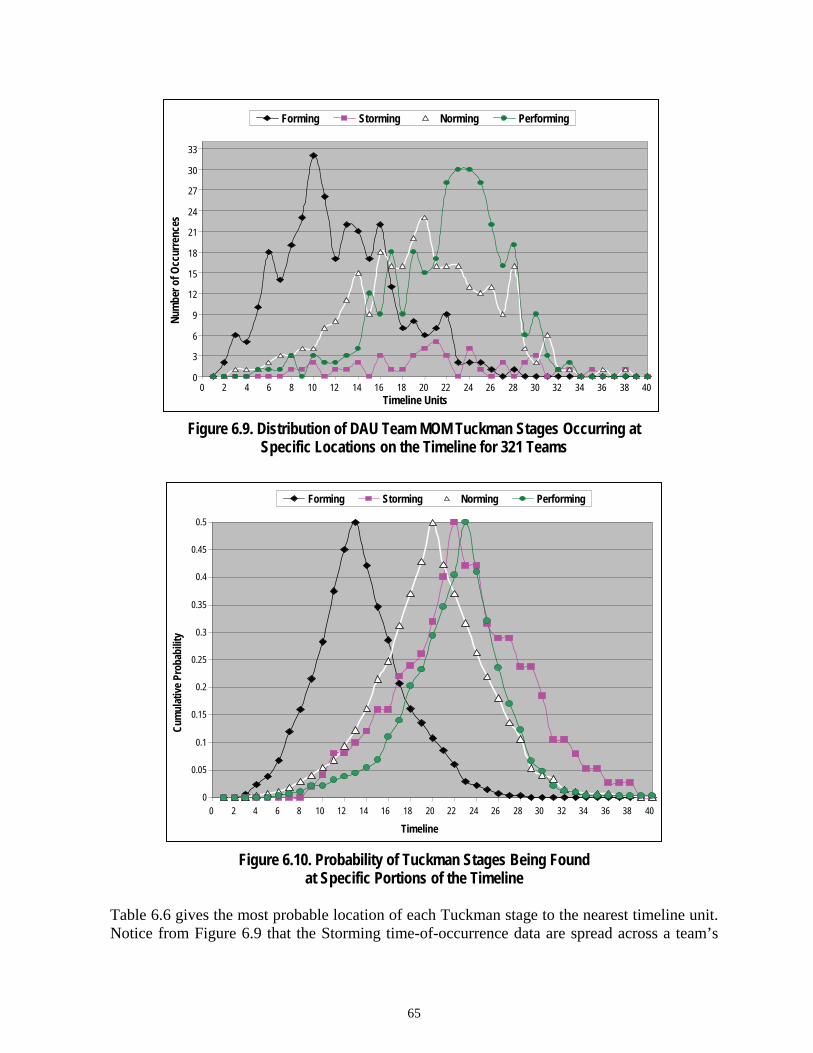
65

0

3

6

9

12

15

18

21

24

27

30

33

0 2 4 6 8 10 12 14 16 18 20 22 24 26 28 30 32 34 36 38 40Timeline Units

Num

ber o

f Occ

urre

nces

Forming Storming Norming Performing

Figure 6.9. Distribution of DAU Team MOM Tuckman Stages Occurring at Specific Locations on the Timeline for 321 Teams

0

0.05

0.1

0.15

0.2

0.25

0.3

0.35

0.4

0.45

0.5

0 2 4 6 8 10 12 14 16 18 20 22 24 26 28 30 32 34 36 38 40

Timeline

Cum

ulat

ive P

roba

bilit

y

Forming Storming Norming Performing

Figure 6.10. Probability of Tuckman Stages Being Found at Specific Portions of the Timeline

Table 6.6 gives the most probable location of each Tuckman stage to the nearest timeline unit. Notice from Figure 6.9 that the Storming time-of-occurrence data are spread across a team’s

66

entire duration more or less evenly. Unlike the other stages, the Storming data do not form a distinct stage location. Of course an average stage time can be calculated for Storming, but it does not represent a clumping of the data around any particular point on the timeline.

Table 6.6. Most Likely Time-of-Occurrence by Tuckman Stage

Forming Storming Norming Performing Time-of-Occurrence 13 22 20 23

Interpreting the Probability Curve: Figure 6.10 tells us that there is a statistical confidence of 95% (P=0.05) that the Forming stage will occur at a point on the timeline that is greater than five timeline units but less than 22.3 timeline units. Similarly, there is a statistical confidence of 95% that the Performing stage will occur at a point on the timeline that is greater than 14 timeline units but less than 30 timeline units. Furthermore, there is a probability of only 0.17 that the Forming and Performing stages will overlap (that Forming will occur at a point on the timeline that is greater than 17.5 or that Performing will occur at a point on the timeline that is less than 17.5). This is equivalent to saying that there is an 83% level of confidence that the Forming and Performing stages will not overlap. There is a 73% level of confidence that the Forming and Norming stages will not overlap and a 62% level of confidence that the Norming and Performing stages will not overlap. Figure 6.9 depicts stages (F<N<P) that are separated by three or more timeline units and one sees that because of the well-defined peaks, consecutive stages are clearly discernable. Summary: From Figures 6.9 and 6.10 it can be seen that, on the average, consecutive stages that are separated by three or more timeline units appear to be discretely separated. In other words, Tuckman events that are separated by three or more timeline units are, on the average, distinguishable as different stages. Approach 3: This approach is the most quantitative; it measured the Probability (Pσ) of obtaining a given value of the standard deviation (σ) for any stage time-of-occurrence measurement generated by the GPQ. The value of Pσ was determined by first sorting all the measured values of σ (standard deviation of the time-of-occurrence data) computed for each team for each stage into time-of-occurrence bins. The resulting distribution of standard deviation data by stage and its associated cumulative probability curves are displayed in Figures 6.11 and 6.12.

67

02468

1012141618202224262830

0 2 4 6 8 10 12 14 16 18 20Standard Deviation in Timeline Units

Num

ber o

f Occ

urre

nces

STDEV (orig data): 3.13 2.31 2.65 2.86Mean (orig data): 8.95 7.71 10.52 9.39Median (orig data): 9.02 7.78 10.58 9.43

Forming Storming Norming Performing

Figure 6.11. Distribution of the Standard Deviation of Time-of-Occurrence Data by Stage

0

0.05

0.1

0.15

0.2

0.25

0.3

0.35

0.4

0.45

0.5

0 1 2 3 4 5 6 7 8 9 10 11 12 13 14 15 16 17 18 19 20

Cum

ulat

ive P

roba

bilit

y

Standard Deviation in Timeline Units

Forming Storming Norming Performing

Figure 6.12. Probability of Occurrence within DAU Data of Various Values of Standard Deviation

The results of this process showed that there was a 0.05 or less probability that any measurement of any stage would exhibit a standard deviation of more than 14.5 timeline units. By modeling time-of-occurrence data curves with a normal distribution with a 14.5 standard deviation, a good estimate of the maximum separation between stage means required to ensure

68

adequate separation between consecutive stages for the “worst case” level of noise was determined. In Figure 6.13, normalized normal distributions with standard deviations of 14.5 model the distribution of the time-of-occurrence data generated by a worst case team given various constant separations between stages. The results of this comparison of MSS values indicate that Tuckman sequences with a separation of three or more timeline units between consecutive stage means would satisfy the requirement that a valid Tuckman sequence must have discrete stages.

Two normalized normal distributions whose means are separated by the constant MSS = 1

00.10.20.30.40.50.60.70.80.9

11.1

0 2 4 6 8 10 12 14 16 18 20 22 24 26 28 30 32 34 36 38 40 42 44 46 48 50

Timeline Units

Normal Dist 1 Normal Dist 2

Two normalized normal distributions whose means are separated by the constant MSS = 3

00.10.20.30.40.50.60.70.80.9

11.1

0 2 4 6 8 10 12 14 16 18 20 22 24 26 28 30 32 34 36 38 40 42 44 46 48 50

Timeline Units

Normal Dist 1 Normal Dist 2

Two normalized normal distributions whose means are separated by the constant MSS = 5

00.10.20.30.40.50.60.70.80.9

11.1

0 2 4 6 8 10 12 14 16 18 20 22 24 26 28 30 32 34 36 38 40 42 44 46 48 50

Timeline Units

Normal Dist 1 Normal Dist 2

Two normalized normal distributions whose means are separated by the constant MSS = 7

00.10.20.30.40.50.60.70.80.9

11.1

0 2 4 6 8 10 12 14 16 18 20 22 24 26 28 30 32 34 36 38 40 42 44 46 48 50

Timeline Units

Normal Dist 1 Normal Dist 2

Figure 6.13. Four Sets of Normal Distributions with Standard Deviation = 14.5 and with Mean Separations of 1, 3, 5, and 7 Timeline Units

Because the justification for setting MSS = 3 is dependent upon claims of reasonableness and are not 100% analytically derived, the results of this research were generated for values of MSS = 0.01, 1, 3, 5, 7, and 9. This parametric assessment (shown in Appendix I) concludes that the results and conclusions relative to the occurrence of the Tuckman sequence F<S<N<P are not at all sensitive to the value of MSS. The variants F<N<P and F<N/P are somewhat more sensitive to changes in MSS but not sensitive enough to change the overall results and conclusions relative to these models even for very wide excursions of the MSS value. In summary, consecutive stages that are separated by three or more timeline units appear to be discernable as unique, discrete stages capable of defining a statistically meaningful sequence. In other words, Tuckman events that are separated by three or more timeline units are

1 2

1 2

1

2

1

2

69

distinguishable as belonging to different stages. Consequently, to effect discrete event separation, a constant value of MSS between stage means belonging to consecutive stages needs to be imposed. Thus, the three conditions for a Tuckman sequence of discrete stage events would be: F ≤ (S - MSS), S ≤ (N - MSS), and N ≤ (P - MSS). It has been shown that setting MSS = 3 provides for a sequence of discrete stages. Therefore the specific conditions for a sequence of discrete Tuckman stages for MSS = 3 become:

F ≤ (S - 3), S ≤ (N - 3), and N ≤ (P - 3)

A parametric analysis of how various values of MSS affect the final results is provided in Appendix I. The results of the parametric analysis indicate that the results and conclusions of this research are not particularly sensitive to small or even moderate changes in the value of MSS. D. A Universal Experience of Tuckman Stages Recall that the second approach to specifying MSS in Section C above began with the calculation of the average location of each Tuckman stage on the 50-unit timeline for each team. Then the frequencies of these average stage locations for each team were distributed on the timeline to produce Figure 6.9. Figure 6.9 does not represent the stage locations of any team, but rather produces a view of all teams in general. It is very interesting that for all DAU teams there appears to be (see Figure 6.10) a common (90% confidence) experience of the Forming stage between 6.5 and 20 timeline units independent of team type or duration. Similarly, Figure 6.10 indicates there was near universal experience (90% confidence level) of Norming occurring between 12 and 28 timeline units and Performing occurring between 16 and 29 timeline units. That unrelated teams experienced the various Tuckman stages at about the same fraction of their duration was an unexpected finding. For the DAU teams, Forming appears to occur at about 25% of the timeline, Norming at about 40% of the timeline, and Performing at about 45% of the timeline. To test this phenomenon more fully, all of the individual event time-of-occurrence data gathered by 1,448 good quality GPQ responses were pooled together as if representing one very large team with 1,448 members who had their own unique but unrelated teaming experiences of various durations. Collectively, this represented over 13,363 pieces of timing data (N) distributed over the stages (ni) as shown in Table 6.7

Table 6.7. Ensemble of 1,448 Individuals—Average Stage Times

Ensemble of Individuals Data Forming Storming Norming Performing Average Stage Time 12.66 22.37 20.23 22.60 Quantity of Time-of-Occurrence Data, ni 3,745 987 4,308 4,323

Note that the average stage times computed for the ensemble of 1,448 individuals are very close to those averaged over teams given in Table 6.6 thus indicating a reasonably accurate roll up of individual team member data into collective team positions. Because large amounts of

70

data were now available to define the time-of-occurrence of each stage, use of the KW test was appropriate. The ni shown in the bottom row of Table 6.7 represents the quantity of time-of-occurrence data defining each stage (the populations of data the Kruskal-Wallis statistic was testing for uniqueness). The average ni equals about 3,341 for the ensemble of all individuals as opposed to the average ni = 9 for DAU teams. Table 6.8 shows the ni values for teams.

Table 6.8. Average Quantity of Time-of-Occurrence Data Per Stage Per Team

The KW test was applied to the ensemble of individuals to determine if the Tuckman stages would be seen as independent (separate and discrete) populations to a confidence level of 95%. The KW test was applied to both four-stage sequences (3 degrees of freedom) and three-stage sequences (2 degrees of freedom). The three-stage assessment was performed on the same dataset as the four-stage assessment except that all the Storming data had been removed.

1. Four-Stage Kruskal-Wallis Assessment

Performing the KW test with the DAU ATO data yielded T = 1562, which is greater than the reference value of 7.815. Thus, the null hypothesis was rejected, indicating that the difference between the means of at least two of the Tuckman stages was statistically significant. Testing for the difference in the means of the time-of-occurrence of each of the Tuckman stages (α = 0.05) revealed that three of the Tuckman stages were significantly different from one another as shown in Table 6.9. Forming and Norming were found to be distinct; however, the difference between Storming and Performing was not statistically significant (α = 0.05). Because the ATO data did not exhibit a Storming peak (Figure 6.9), one would not expect the KW test to find a separate Storming stage. Furthermore, from Table 6.7 the average Storming time-of-occurrence is only separated by 0.23 timeline units from the Performing ATO, which would make it likely that the Storming data would be grouped with the Performing stage data. The KW test result, F<N<S/P, indicates that if the Storming data were discounted, the ensemble would universally perceive a common F<N<P sequence of discrete separate events. It appears that an ensemble of all DAU team members from all teams does, to some extent, collectively experience a similar sequence of the F, N, and P Tuckman stages at about the same fraction of their team’s duration. This result raises the possibility of a common experience of Tuckman stages at predictable intervals independent of team task or team duration.

Time-of-Occurrence Data For Teams Forming Storming Norming Performing

The average number of time-of-occurrence data points (ni) that a single

team produces for each stage? 10.20 2.69 11.74 11.78

71

Table 6.9. Kruskal-Wallis Stage Differences Four-Stage

Stage Comparisons

ji

i j

RRn n

⋅ ( )

11 222

1 2

1 1 1a

i j

N Tt SN k n n−

⎛ ⎞− −⎛ ⎞ +⎜ ⎟⎜ ⎟ ⎜ ⎟−⎝ ⎠ ⎝ ⎠ Difference

Forming vs. Storming 3055.8 255.5 Yes

Forming vs. Norming 2422.5 159.5 Yes

Forming vs. Performing 3218.5 159.4 Yes

Storming vs. Norming 633.3 252.0 Yes

Storming vs. Performing 162.7 251.9 No

Norming vs. Performing 796.0 153.7 Yes

2. Three-Stage Kruskal-Wallis Assessment

A three-stage version of the Kruskal-Wallis test was also applied to the DAU ensemble of all individuals from all teams to determine if the F<N<P sequence could be separated into discrete stages. The DAU ATO data with two degrees of freedom yielded a reference value of 2

2χ = 5.991 and T = 1466. Since T was greater than the reference value, the null hypothesis was rejected, indicating that the difference between the means of at least two of the three stages is statistically significant. Testing for the difference in the means of the time-of-occurrence of each of the three stages (α = 0.05) revealed that all three of the stages were significantly different from one another as shown in Table 6.10.

Table 6.10. Kruskal-Wallis Stage Differences Three-Stage

Stage Comparisons

ji

i j

RRn n

⋅ ( )

11 222

1 2

1 1 1a

i j

N Tt SN k n n−

⎛ ⎞− −⎛ ⎞ +⎜ ⎟⎜ ⎟ ⎜ ⎟−⎝ ⎠ ⎝ ⎠ Difference

Forming vs. Norming 2233.34 147.55 Yes

Forming vs. Performing 2967.93 147.43 Yes

Norming vs. Performing 734.59 142.18 Yes

As expected, the time-of-occurrence data representing the Forming, Norming, and Performing stages do (to a 95% level of confidence) appear to be from different populations indicating that

72

the ensemble of 1,448 individuals perceives the F<N<P model as a sequence of discrete stages. This can only happen if stages more or less universally occur at about the same fraction of the timeline for all teams. The Kruskal-Wallis analysis is consistent with the analysis of raw timing data, which indicate that Forming occurs at about 25% of a team’s duration, Norming occurs at approximately 40% of a team’s duration, and Performing occurs near 45% of a team’s duration. E. Defining Statistically Valid Teaming Experience 1. Introduction This research uses two statistical requirements each with its own statistical criteria that must be imposed upon the analysis methodology to ensure that the results are scientifically credible. The first statistical requirement provides the confidence level that the results are derived from signal, or equivalently, not derived from noise. The first requirement ensures a statistically valid teaming experience is one that can be proven to a 95% level of confidence to be derived from accurate and meaningful information measured by the GPQ. That is, each team’s qualitative and quantitative experience of a given sequence of Tuckman events (as measured by the GPQ) must be shown to be very unlikely (P ≤ 0.05) to have occurred as a result of random fluctuations in the data (noise). To meet the first requirement, an analysis of the sequences defined by the answers to the questionnaire was undertaken. This methodology is called Sequence Analysis. Secondly, there is a requirement that consecutive stages experienced by the team must be (to a 95% confidence level) separate discrete stages. This second statistical requirement is imposed to make sure that overlapped and commingled consecutive stages that have stage means separated by less than the measurement resolution of the instrument (for stage location) do not constitute a valid sequence. If consecutive stage separation is too small relative to noise levels and measurement capability, it would be impossible to determine (to a 95% confidence level) which stage preceded which, and no valid sequence is defined. The MSS described in Section B above was used to meet this statistical requirement. All results and conclusions offered by this research are based upon statistically validated team and individual data. This section discusses the analysis employed to validate team and individual experiences in support of the three models of interest: F<S<N<P, F<N<P, and F<N/P. The fundamental issues underlying both statistical requirements, and the ability of the Miller (1997) GPQ instrument to provide the necessary data to adequately resolve each, are discussed in Chapter IV and Appendices J and N. 2. Satisfying Statistical Requirement 1: Sequence Analysis (SA) As defined earlier in this research, let the letters F, S, N, P represent the mean time-of-occurrence of Forming, Storming, Norming, and Performing events respectively. There were three Forming questions Fi = {F1, F2, F3}, where i = 1, 2, 3. There were four Storming questions Sm = {S1, S2, S3, S4}, where m = 1, 2, 3, 4. There were four Norming questions Nj =

73

{N1, N2, N3, N4}, where j = 1, 2, 3, 4. And there were four Performing questions Pk = {P1, P2, P3, P4}, where k = 1, 2, 3, 4. If a Tuckman event was observed (indicated by a team member answering “YES” to one of the Tuckman questions), the subject was required to indicate on a timeline when that event occurred. Thus, each member of each team indicated which Tuckman event they observed and when that event occurred during their teaming experience to the nearest 1/50 of the duration of the teaming experience. Each event could be given one or multiple time-of-occurrence observations by each team member. If a respondent had more than one time-of-occurrence observation selected, the data had to be combined. The data were combined by averaging the time-of-occurrence values. Averaging was also used to combine team member timing data for each question to form a collective team experience such that every Tuckman event collectively observed by each team had one associated mean time-of-occurrence. a. Counting Tuckman Sequences. Using the notation defined above, it should be clear that for all possible values of the subscripts, Fi < Sm < Nj < Pk implies that the three times-of-occurrence for the three Forming questions are less than (occur before) the four times-of-occurrence associated with the four Storming questions … and so on. If all 15 Tuckman questions were answered “YES,” and if Fi < Sm < Nj < Pk for all values of i, m, j, k, there are exactly 192 unique Tuckman sequences that could be defined. 3 x 4 x 4 x 4 = 192. In other words, there are 192 possible ways that the answers to the 15 Tuckman questions can support a Tuckman sequence (F<S<N<P). Both the sequences of Tuckman events produced by individuals as well as those produced by teams were evaluated using the SA methodology. Let SAF<S<N<P represent a logical algorithm that allows the researcher to determine what percentage of the sequences generated by individuals and teams were Tuckman sequences. The Tuckman score (FSNP-score) is defined as the percentage of the 192 possible Tuckman sequences that a team or an individual generated based upon the time-of-occurrence data produced for each of the 15 Tuckman questions. Appendix J provides more detail on how FSNP-Scores were computed with the SAF<S<N<P logical algorithm. Consider Figure 6.14: If I = 1, m = 3, j = 2, and k = 4, the sequence F1<S3<N2<P4 is defined, which is one of the 192 possible sequences, wherein the time-of-occurrence of the first Forming question (F1) is less than the time-of-occurrence of the third Storming question (S3), which in turn has a time-of-occurrence that is less than the second Norming question (N2), which in turn has a time-of-occurrence that is less than the fourth Performing question (P4). F1<S2<N4<P3 is another one of the 192 possible sequences and F3<S2<N3<P2 is yet another.

74

Figure 6.14. Fifteen (3 + 4 + 4 + 4) Questions Produce 192 (3 x 4 x 4 x 4) Possible Tuckman Sequences

Given the set of answers and corresponding time-of-occurrence data generated by an individual team member, or after all team members’ data have been coalesced into a single collective team position for each of the 15 questions, one can calculate how many of the 192 possible Tuckman sequences (Fi<Sm<Nj<Pk) were experienced by that individual or team. This number divided by 192 and multiplied by 100 gives the percent of all possible Tuckman sequences that the individual or team experienced. This percentage is defined as that individual’s or team’s Tuckman score or FSNP-Score.

b. Deriving Significance Thresholds A Monte Carlo simulation was used to generate a reference distribution of Tuckman scores. A Large number (102,000) of questionnaires were filled out randomly—i.e., Randomly answering “YES,” “NO,” or “UNCERTAIN” to each of the 15 Tuckman questions and then producing random times-of-occurrence for each “YES” answer. A Tuckman score was calculated for each of the 102,000 random teams. A reference distribution was generated for these FSNP-Scores by sorting the 102,000 random FSNP-Scores into 100 bins. For example, all the FSNP-Scores between 15.5 and 16.499 were counted and that number was put into bin 16. Because accuracy improves with the number of samples generated, the number of samples used (102,000) simply reflects the practical limits of the available computing resources. Next, integrating over the distribution produced a cumulative probability curve. This probability curve was then used to generate a numerical level of confidence that a given score was not produced by random data. Obviously, very low FSNP-Scores requiring little specific organization of the input values are more easily produced by random inputs and very high FSNP-Scores (requiring all F times to be less than all S times, etc.) are nearly impossible to produce from 15 random inputs created by a random number generator.

F 1 F 2 F 3

S1 S2 S3 S4

N 1 N 2 N 3 N 4

P1 P2 P3 P4

3 Forming

4 Norming

4 Performing

F 1 F 2 F 3 F 1 F 1 F 2 F 2 F 3 F 3

S1 S2 S3 S4 S1 S1 S2 S2 S3 S3 S4 S4

N 1 N 2 N 3 N 4 N 1 N 1 N 2 N 2 N 3 N 3 N 4 N 4

P1 P2 P3 P4 P1 P1 P2 P2 P3 P3 P4 P4

3 Forming

4 Storming

4 Norming

4 Performing

75

Each FSNP-Score produced by the DAU data was required to be larger than the random FSNP-Score associated with a αSA = 0.05 probability (of being produced by random processes) in order to be declared “significant.” In other words, for an FSNP-Score generated by a DAU team to be considered statistically significant, it must be large enough such that the probability of that score being produced by random input data is less than 0.05. To summarize: An individual’s or team’s FSNP-Score was counted as being supportive of the Tuckman model only if its value was equal to or greater than the calculated “significance threshold.” The significance threshold is an FSNP-Score calculated within the SA algorithm associated with a probability of 0.05 that a given FSNP-Score could have been generated by random inputs. From the random reference distribution and its associated cumulative probability curve, it was determined that an FSNP-Score of 0.0976 had a probability of 0.05 of being random. Thus any score equal to, or greater than, 0.0976 represented a significant score. Appendix J provides more detail on random Tuckman score distributions and probability curves. The two variants of the Tuckman sequential stages model, F<N<P and F<N/P, were assessed using the same analytical methodology. In the exact same manner described above for creating an SA algorithm SAF<S<N<P that calculates FSNP-Scores in order to assess the degree to which a statistically valid Tuckman model (F<S<N<P) was experienced by DAU teams, an SAF<N<P algorithm was developed that calculates FNP-Scores in order to assess the degree to which a statistically valid F<N<P model was experienced by DAU teams. Similarly, an SAF<N/P algorithm was developed that calculates FN/P-Scores in order to assess the degree to which a statistically valid F<N/P model was experienced by DAU teams. The significance threshold for F<N<P sequences was 4.251, and the significance threshold for F<N/P sequences was 6.511. Appendix J.2 and Appendix J.3 provide more detail on F<N<P and F<N/P distributions and SA calculations. A parametric analysis of how various values of αSA = 0.05, 0.1, 0.15, 0.2, and 0.25 affect the final results is provided in Appendix I. Also, Appendix I shows how the significance thresholds vary as a function of MSS (Figure I.1) and αSA (Figure I.2). 3. Satisfying Statistical Requirement 2: Discrete Stage Analysis The MSS analysis was used to satisfy this statistical requirement. Three independent approaches were used to determine that a separation of three timeline units was sufficient to ensure discrete stage separation to a 95% level of confidence. The three conditions that must be met in order to define a sequence of discrete Tuckman stages can be stated as:

Fi ≤ (Sm - 3), Sm ≤ (Nj - 3), and Nj ≤ (Pk - 3)

These conditions were integrated into the logical SA algorithms that defined FSNP-Scores, FNP-Scores, or FN/P-Scores for a given individual or team. Individuals and teams that satisfied both conditions were statistically validated. Individuals and teams that did not satisfy both conditions were dropped out of the analysis process at this

76

point to become counted as individuals and teams that did not follow the Tuckman model. In this last group were those who never experienced the Tuckman model and those who may have experienced the Tuckman model in some vague and minor way but not solidly enough to rise above the noise or achieve statistical credibility as having done so. 4. Assessing Stage Sequence: An Optional More Restrictive Validation Requirement One can go a step further and require that each team or individual experience the average Tuckman stage times-of-occurrence in the proper order. The difference lies between how event times-of-occurrence and stage times-of-occurrence are defined. To say a team is statistically validated means that its teaming experience of F<S<N<P, F<N<P, or F<N/P, as measured in terms of Tuckman events by the Miller GPQ, is verified to be scientifically credible. This means that the team has implicitly experienced a statistically validated Tuckman development sequence of event-stages. There is no need to compute a mean time-of-occurrence for each stage in order to determine if a team is statistically valid—i.e., one only needs to define a mean time-of-occurrence for each observed Tuckman event to determine statistical significance. Recall that each question in the GPQ describes a Tuckman event. Team members place marks on the timeline to indicate when various Tuckman events occurred. All the Tuckman events belonging to the same question are averaged to provide input for the SA algorithm as described above. When all the Tuckman events belonging to the same stage have their times-of-occurrence averaged, they produce a mean time-of-occurrence for that stage. That is, a stage time is computed by averaging all of the event times generated by each team member for a given stage. However, SA scores are computed using average event times for each question not for each stage. Because the Tuckman model is a stage model not an event model (even though each event is stage-specific), one may wish to verify that the statistically validated individuals and teams did indeed experience the Tuckman model by determining the ATO of each stage and then verifying that the stages occurred in the required sequence (F<S<N<P, F<N<P or F<N/P). Assessing the explicit experience of the Tuckman model (F<S<N<P) imposes an extra (unnecessary) constraint upon a team’s measured developmental process in order to make a “most conservative” comparison with the accepted results of SA alone. Implicit and explicit results are compared in Appendix I under a variety of circumstances. 5. Statistical Validation Summary The SA algorithm only requires that statistically validated teams experienced enough sequences of Tuckman events among their question data to be statistically significant (results not derivable from random fluctuations) and that those Tuckman events represent discrete consecutive events (separated by at least 3 timeline units) that are not smeared together within some non-differentiable mass of event data. Thus, statistical validation for a given model like F<S<N<P, F<N<P, or F<N/P, which is based upon the ATO of the event described by each question, can occur without a team experiencing the proper sequence of Tuckman stages,

77

which are defined by averaging the event time-of-occurrence data over all questions belonging to the same stage. To create a more robust test to assess the Tuckman model, a more restrictive validation process that goes beyond the requirements of statistical rigor could determine how many of the statistically validated individuals and teams also experienced average stage time-of-occurrences in the F<S<N<P sequence. Similarly, a more restrictive validation process for the F<N<P and F<N/P variants may also be performed. The results of these more restrictive validation processes will be reported along with the results of the statistical analysis produced by SA so that comparisons can be made. F. Overall Summary of Analytical Methodology and Numerical Process A Kappa analysis of the level of agreement between team members’ answers to the Miller (1997) GPQ indicated that the team members clearly understood what they were experiencing within their teams and had no trouble relating that experience to the questionnaire instrument. (This is discussed in more detail in Chapter V and Appendix N.) A variance analysis determined that the timing data collected by the Miller GPQ was able to accurately detect and measure discrete Tuckman stages separated by as few as three timeline units. (This is discussed in more detail in Chapter V, Chapter VI, and Appendix N.) Four types of automated data quality filters were defined. Each filter was carefully designed to eliminate a particular type of “noise” from the collected data. Noise sources and misleading data, if not effectively eliminated, were shown to introduce errors of 15% to 20% in the results. (This is discussed in more detail in Chapter V and Appendix M.) It was shown that if consecutive Tuckman stages were separated by three or more timeline units, one could be 95% confident that, in general, these stages represented discrete separate entities capable of forming a well-defined sequence. Furthermore, it was shown that this requirement could be easily integrated with the logical algorithm used in defining SA scores for each model studied (FSNP-Score, FPN-Score, and FN/P-Score). A method of SA was devised that determined the percentage of possible Tuckman sequences (FSNP-Score) that each team or individual generated from the data collected by the GPQ. A reference distribution was generated to define a statistical significance threshold for FSNP-Scores. It was demonstrated that any FSNP-Score that was greater than this threshold value had less than a 0.05 probability of being the result of random processes. It was demonstrated that the information content of the collected data had a high enough signal-to-noise ratio to support scientific credibility and that the analysis methodology enforced both of the statistical requirements necessary to fully validate the sequences upon which the results were based. A similar methodology was used to statistically assess the meaningfulness of the F<N<P and F<N/P models as well. Combining the FSNP-Score criteria and the MSS criteria into the SA process fully satisfied and implemented the two fundamental statistical requirements that together support a

78

statistically rigorous analysis. The first requirement ensured that the results of this research (to a numerical level of confidence specified by αSA = 0.05) could not be obtained from the analysis of random input data. The second requirement ensured that the results of this research (to a level of confidence specified by ασ = 0.05) were clearly derived from sequences of discrete Tuckman stages. The results of this research are derived only from data that fully satisfy both requirements. Evidence for a universal or common experience of the F, N, and P stages at 25%, 40%, and 45% of a team’s duration (regardless of team activity or duration) was presented for team data and then verified by individual data using the KW test for population uniqueness. An additional requirement that the ATO of stages follow the model being assessed was discussed as an optional criteria for more strictly assessing team and individual results. Results are reported using both sets of criteria. Because choice of methodology can impact results, it was extremely important to carefully evaluate how the individual question data were coalesced into a collective team position. Competing methodologies were analyzed, accuracy was assessed, and sensitivity analyses were conducted to select the best (most accurate, transparent, and introduces minimum dispersion in the data) methods for each step in the data reduction process. Three alternative team views of the same data—Team IRA, Team UTD, and Team MOM—were defined. A fourth alternative view of the data was in terms of the teaming experience of each of the 1,448 individual team members. Team IRA uses an IRA methodology to determine collective answers to the questionnaire. Team UTD collects together the unconstrained team (raw) data from each of its members and simply averages all of the individual times-of-occurrence for each stage. Team MOM applies some additional criteria to the UTD data (a MOM that tests the quality of the data representing each stage) to make sure that collective event and stage times-of-occurrence accurately represent the team’s overall experience. Details of the criteria enforced by the MOM process and a discussion of results in terms of alternative views can be found in Appendix L. All of the alternative analysis approaches produced results that were compatible with, supportive of, and similar to the results and conclusions of this research. That several independent approaches reached more or less the same conclusions gives weight to the accuracy of the methodology and analysis and to the strong signal-to-noise ratio of the measured data. All key analytical assumptions were represented by variable input parameters that enabled the researcher to understand how the choice of each parameter affects the accuracy of the calculations and the final results. If the results were shown to be sensitive to a given parameter, then the utmost care was taken to specify such a parameter precisely or multiple sets of outputs spanning the outer limits of reasonability were used to produce a range of plausible results. A parametric analysis of how certain parameters (MSS, αSA, average vs. median, etc.) affected the final results is provided in Appendix I.

79

G. Results 1. How Well did DAU Teams Follow the Tuckman Model or Either of its Variants? As mentioned elsewhere, Team MOM represents the analysis configuration of team data that most accurately reflects each team’s experience as measured by the GPQ. Team MOM results and only Team MOM results represent the final results or output of this research of small, short duration technical team development. The results of assessing individuals and other team analysis configurations (Team UTD and Team IRA) provide a more well-rounded understanding of the results, facilitate comparisons to other research, and are presented here for comparisons only. The final results are shown in Table 6.11. To make sure that this results table is clearly understood, a description of the Team MOM result for the F<N<P three-stage sequence (area being discussed in table is double-bordered). Every other section of the table follows the exact same interpretation as those given in this example. F<N<P is a three-stage model defined as “Tuckman Variant 1.” The F<N<P sequence as experienced by the 321 DAU teams with the MOM factor applied produced 158 (49.22%) “Natural” F<N<P sequences. “Natural” simply means that the teams directly reported experiencing 158 F<N<P sequences from the raw timing data. Additionally, these 321 teams reported 9 other sequences that collapsed to an F<N<P sequence once Storming was removed. For example S<F<N<P and F<S<N<P and F<N<S<P and F<N<P<S all collapse to F<N<P when the “S” is removed (as if the Storming questions were eliminated from the questionnaire) to test a three-stage alternative model of Forming, Norming, and Performing. This produced a total of 167 (52.02%) F<N<P timing sequences (i.e., 167 F<N<P sequences were experienced by the 321 teams). Of these 167 F<N<P sequences, 6 (1.87%) were not found to be statistically significant [their FSNP-Scores were too low (less than a 95% confidence that their event sequences were not derivable from random inputs) and/or their stage means occurred too close together to have a confidence of ≥ 95% that they were indeed discrete stages)]. That left (167 - 6) = 161 statistically validated F<N<P sequences that also met the additional requirement that their stages were in the correct F<N<P order. There were 229 teams (71.34% of the total 321 teams) deemed to have passed both statistical tests by producing a significant “Tuckman Variant 1 score (FNP-Score ≥ 4.251) where 4.251 was the αSA = 0.05 significance threshold for the SAF<N<P Algorithm) and by having means of its F, N, and P events separated by at least 3 timeline units.

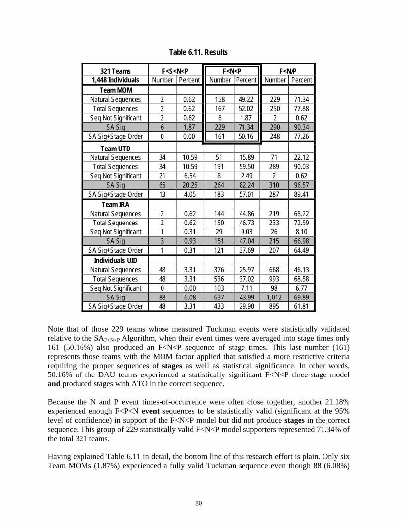
80

Table 6.11. Results

321 Teams F<S<N<P F<N<P F<N/P 1,448 Individuals Number Percent Number Percent Number Percent

Team MOM Natural Sequences 2 0.62 158 49.22 229 71.34 Total Sequences 2 0.62 167 52.02 250 77.88

Seq Not Significant 2 0.62 6 1.87 2 0.62 SA Sig 6 1.87 229 71.34 290 90.34

SA Sig+Stage Order 0 0.00 161 50.16 248 77.26 Team UTD

Natural Sequences 34 10.59 51 15.89 71 22.12 Total Sequences 34 10.59 191 59.50 289 90.03

Seq Not Significant 21 6.54 8 2.49 2 0.62 SA Sig 65 20.25 264 82.24 310 96.57

SA Sig+Stage Order 13 4.05 183 57.01 287 89.41 Team IRA

Natural Sequences 2 0.62 144 44.86 219 68.22 Total Sequences 2 0.62 150 46.73 233 72.59

Seq Not Significant 1 0.31 29 9.03 26 8.10 SA Sig 3 0.93 151 47.04 215 66.98

SA Sig+Stage Order 1 0.31 121 37.69 207 64.49 Individuals UID

Natural Sequences 48 3.31 376 25.97 668 46.13 Total Sequences 48 3.31 536 37.02 993 68.58

Seq Not Significant 0 0.00 103 7.11 98 6.77 SA Sig 88 6.08 637 43.99 1,012 69.89

SA Sig+Stage Order 48 3.31 433 29.90 895 61.81 Note that of those 229 teams whose measured Tuckman events were statistically validated relative to the SAF<N<P Algorithm, when their event times were averaged into stage times only 161 (50.16%) also produced an F<N<P sequence of stage times. This last number (161) represents those teams with the MOM factor applied that satisfied a more restrictive criteria requiring the proper sequences of stages as well as statistical significance. In other words, 50.16% of the DAU teams experienced a statistically significant F<N<P three-stage model and produced stages with ATO in the correct sequence. Because the N and P event times-of-occurrence were often close together, another 21.18% experienced enough F<P<N event sequences to be statistically valid (significant at the 95% level of confidence) in support of the F<N<P model but did not produce stages in the correct sequence. This group of 229 statistically valid F<N<P model supporters represented 71.34% of the total 321 teams. Having explained Table 6.11 in detail, the bottom line of this research effort is plain. Only six Team MOMs (1.87%) experienced a fully valid Tuckman sequence even though 88 (6.08%)

81

out of 1,448 individuals experienced a valid Tuckman sequence. Obviously, many of these individuals were not on the same teams. Of the six teams that experienced a valid Tuckman sequence, none produced average stage time-of-occurrences in the correct F<S<N<P order. DAU teams did not follow the Tuckman four-stage model of F<S<N<P to any appreciable degree. A little more than 71% of the DAU teams experienced a valid Tuckman model Variant 1 (F<N<P) sequence of Tuckman stages, while over 90% of the DAU teams experienced a valid Tuckman model Variant 2 (F<N/P) sequence of stages. 2. Other Considerations—Individuals, Team UTD, and Team IRA Without a MOM to toss out spurious data, Team UTD results indicated many more Tuckman sequences than the other team characterizations. Of the 65 statistically validated Team UTDs following the Tuckman model, only 6 actually experienced enough Storming to be meaningful. The other 59 were the result of noisy non-representative data and carry no meaning. Notice that Team UTD produced few natural F<N<P or F<N/P sequences compared to the others because the large amount of non-representative Storming produced more natural four-stage sequences and fewer three-stage sequences. Evidently, quite a few teams had one or two Storming events that were determined by the MOM to be spurious data. When all the Storming data were tossed out in order to assess three (F<N<P) and two (F<N/P) stage models, Team UTD still outproduced Team MOM because the MOM algorithm eliminated spurious data from all stages, not just Storming. Though the preponderance of spurious data was found in the Storming stage, all stages were occasionally affected. Notice that Team IRA consistently sees fewer sequences than Team MOM in almost all categories. That is because the IRA algorithm that wholly defines Team IRA is just one of three criteria in the MOM calculation. Since MOM is a logical OR spanning three criteria, it is less restrictive (has two other possible paths to success) than the single IRA criteria defining Team IRA. It is also interesting to note that the team development experience of individuals remains spread out over more varied sequences and is not as likely to clump into F<N<P and F<N/P structures like the averaged team data do. This makes the individuals look more like Team IRA than the other two team characterizations. The most important thing to notice here is that all analytical configurations of the data (all three team characterizations and individuals) generally come to similar conclusions: The Tuckman model has almost no support while there is significant support for the Tuckman variant F<N<P and even more support for the simple two-stage model F<N/P. Team MOM represents the best analytical team configuration and the most accurate results. 3. Comparison of the DAU Results with the Results of Other Research Both Miller (1997) and Benfield (2005) employed a data collection methodology that was similar to the data collection methodology used by this research. Furthermore, Benfield (2005) studied technical teams drawn from the same DoD acquisition environment that spawned the

82

DAU teams. Given these similarities, one might assume that strong comparisons could be made between these three research projects that would shed light on both the efficacy of the methodology and the consistency of results. Unfortunately, because of the complete dissimilarity in data analysis methodology, it is difficult to compare the results of this research with either Miller’s or Benfield’s results. Although a comparison of the results of this research with Benfield’s (2005) results is problematical, a comparison of Benfield’s data with the DAU data, as is done in this chapter and in Chapter IV, may be valuable as long as one looks at generalities and not detail. Neither Benfield (2005) nor Miller (1997) assessed the F<N<P or F<N/P variants of the Tuckman model. As expected, Team UTD, because of the greatly increased weighting it gives to spurious or unrepresentative Storming data, saw 65 (20.25%) of its teams support the F<S<N<P Tuckman model. This value is a little less than half way between the 36% Tuckman following reported by Miller (1997) and the 13% Tuckman following reported by Benfield. However, it is 10 times greater than the more accurate 2% reported by this research for Team MOM. Miller (1997) used the FTO data aggregating methodology (a process that is shown in Appendix L to be relatively noisy) to assess her role playing teams (21 teams of college students in an organizational theory course playing the role of corporate officers). It is of interest to note that of the 65 statistically validated DAU Team UTDs observing the Tuckman model, only 13 produced stages in the correct order. Since Miller (1997) and Benfield only evaluated stage order and did not require any statistical validation of the sequences reported by their teams, an assessment similar to theirs would have reported that 13 of the DAU teams (4.05%) followed the Tuckman model. Because of the dissimilarity in analysis methodology, and the small number of independent teams studied by Miller, it is difficult to compare the results of this research with those produced by Miller and Benfield. Like Miller, Benfield (2005) evaluated only stage order and did not impose any statistical requirements on the team sequences he reported. Furthermore, he aggregated time-of-occurrence data using the median which has been shown (Appendix L) to introduce additional noise into the analysis process. Moreover, no quality filtering of the input data was used to eliminate noise, errors, and misinformation from the data. Furthermore, 53% of Benfield’s (2005) teams were reported to have durations of greater than 1 year. Three possibilities exist: 1) the teams were still in process (had not completed their tasks) when the GPQ was filled out; or 2) team members were asked to remember specific events and the time these events occurred many months after the fact; or 3) perhaps the task of these long duration teams was ongoing and not discrete. The first and third possibilities represent situations for which the GPQ was not designed. All three cases represent sub-optimal conditions for collecting data via the GPQ and would appear to introduce noise and imprecision into the data. Whether or not Benfield’s other teams (with durations smaller than 1 year) fell into one or more of these three issue categories is unknown. Though Benfield attempted to use the KW test to validate the discreteness or separateness of consecutive stages within a sequence, this test is not suitable for the task because of small N combined with very noisy data. The noisy data is the major issue; small N simply prevented noise reduction through averaging from being effective. In Appendix K it is demonstrated that

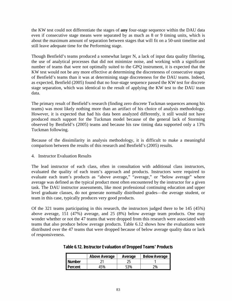
83

the KW test could not differentiate the stages of any four-stage sequence within the DAU data even if consecutive stage means were separated by as much as 8 or 9 timing units, which is about the maximum amount of separation between stages that will fit on a 50-unit timeline and still leave adequate time for the Performing stage. Though Benfield’s teams produced a somewhat larger N, a lack of input data quality filtering, the use of analytical processes that did not minimize noise, and working with a significant number of teams that were not optimally suited to the GPQ instrument, it is expected that the KW test would not be any more effective at determining the discreteness of consecutive stages of Benfield’s teams than it was at determining stage discreteness for the DAU teams. Indeed, as expected, Benfield (2005) found that no four-stage sequence passed the KW test for discrete stage separation, which was identical to the result of applying the KW test to the DAU team data. The primary result of Benfield’s research (finding zero discrete Tuckman sequences among his teams) was most likely nothing more than an artifact of his choice of analysis methodology. However, it is expected that had his data been analyzed differently, it still would not have produced much support for the Tuckman model because of the general lack of Storming observed by Benfield’s (2005) teams and because his raw timing data supported only a 13% Tuckman following. Because of the dissimilarity in analysis methodology, it is difficult to make a meaningful comparison between the results of this research and Benfield’s (2005) results. 4. Instructor Evaluation Results The lead instructor of each class, often in consultation with additional class instructors, evaluated the quality of each team’s approach and products. Instructors were required to evaluate each team’s products as “above average,” “average,” or “below average” where average was defined as the typical product most often encountered by the instructor for a given task. The DAU instructor assessments, like most professional continuing education and upper level graduate classes, do not generate normally distributed grades—the average student, or team in this case, typically produces very good products. Of the 321 teams participating in this research, the instructors judged there to be 145 (45%) above average, 151 (47%) average, and 25 (8%) below average team products. One may wonder whether or not the 47 teams that were dropped from this research were associated with teams that also produce below average products. Table 6.12 shows how the evaluations were distributed over the 47 teams that were dropped because of below average quality data or lack of responsiveness.

Table 6.12. Instructor Evaluation of Dropped Teams’ Products

Above Average Average Below Average Number 21 25 1 Percent 45% 53% 2%

84

It should be noted that dropping a team from the research database because of below average response and/or below average quality data is not an indicator of below average performance. In fact, the data indicate that teams with average performance were a little more likely to be dropped while teams with below average performance were less likely to be dropped. Another concern is whether or not teams that Storm produce below average products. Table 6.13 shows how team performance evaluations were distributed over those 44 (14%) teams out of 321 that observed significant Storming. The data indicate that a team that Storms much more than usual is not an indicator of below average performance. In fact, the percentage of Storming decreases as team performance decreases.

Table 6.13. Instructor Evaluation of Products of Teams Observing Storming

Above Average Average Below Average Number 21 19 4 Percent 48% 43% 9%

Additionally, it is important to determine if there was a significant correlation between those teams observing statistically significant F<S<N<P, F<N<P or F<N/P sequential stage models and the teams’ performance as assessed by the class instructor. To be more specific, the question was: Of the Team MOMs receiving a particular instructor assessment (above average, average, or below average), what percentage produced an output SA sequence of F<S<N<P, F<N<P or F<N/P? Table 6.14 provides the data that answer that question for all three models.

Table 6.14. Instructor Evaluation vs. Teams Producing Statistically Significant Sequences

Sequence Rating Number Percent Above Average (145) 6 4.14%

Average (151) 0 0 F<S<N<P Below Average (25) 0 0

Above Average (145) 114 78.62% Average (151) 102 67.55% F<N<P

Below Average (25) 13 52% Above Average (145) 138 95.17%

Average (151) 131 86.75% F<N/P Below Average (25) 21 84%

From Table 6.14, 4.14% of the 145 above average teams produced a statistically significant FSNP-Score for the F<S<N<P sequence. Note that all six of the F<S<N<P sequences that passed the SA logical algorithm produced above average products.

85

From Table 6.14, it can be seen that for all three sequences models, above average teams produced the most statistically significant results followed by average teams, while below average teams produced the fewest statistically significant results. The table shows consistent descending stairstepped results in quantity of sequences generated for each team dynamics model as the teams’ rating moves from above average to below average. A chi square r x c contingency test was performed to determine the correlation between instructor assessment and a team’s probability of producing one of the three sequences of Tuckman stages (F<S<N<P, F<N<P or F<N/P). The results are shown in Table 6.15.

Table 6.15. Correlation between Team Performance and Team Development Model Followed

Sequence F<S<N<P F<N<P F<N/P Correlation 0.95 0.99 0.95

The correlation numbers given in Table 6.15 are the probabilities that the populations are not independent—i.e., the probability that there is a relationship between a team’s performance and the model of team development followed by that team. Correlations of 0.95 or greater are considered to represent a relationship between populations that is statistically significant. The more productive and successful a team was, the more likely they were to observe one of the three sequences of Tuckman stages assessed by this research. A strong correlation between team performance and the model of team development followed is important enough that one might ask if this association was just some fluke related to Team MOM or would all team analytical structures exhibit the same behavior? To be more specific, the question is: Of the Team IRA and Team UTD receiving a particular instructor grade (above average, average, or below average), what percentage produced a final output sequence of F<S<N<P, F<N<P or F<N/P? Figures 6.15, 6.16, and 6.17 answer that question for all three models.

86

0.00

5.00

10.00

15.00

20.00

25.00

30.00

35.00

Team IRA Team UTD Team MOM

Perc

ent P

rodu

cing

F<S<

N<P

Above Ave Average Below Ave

Figure 6.15. Instructor Evaluation vs. Percent of Teams Producing

Statistically Significant F<S<N<P Sequences

0.00

20.00

40.00

60.00

80.00

100.00

120.00

Team IRA Team UTD Team MOM

Perc

ent P

rodu

cing

F< N

/P

Above Ave Average Below Ave

Figure 6.16. Instructor Evaluation vs. Percent of Teams Producing Statistically Significant F<N<P Sequences

87

0.00

10.00

20.00

30.00

40.00

50.00

60.00

70.00

80.00

90.00

100.00

Team IRA Team UTD Team MOM

Perc

ent P

rodu

cing

F<N<

P

Above Ave Average Below Ave

Figure 6.17. Instructor Evaluation vs. Percent of Teams Producing Statistically Significant F<N/P Sequences

It can be seen for all three Team characterizations (except Team UTD experiencing F<S<N<P) that above average teams produced the most statistically significant results followed by average teams, while below average teams produced the fewest statistically significant results A chi square r x c contingency test was performed to determine the correlation between grade received and a team’s probability of producing one of the three sequences of Tuckman stages (F<S<N<P, F<N<P or F<N/P). The correlation for each team characterization vs. each sequence is given in Table 6.16.

Table 6.16. Overall Correlation between Team Performance and Team Development Model Followed for Three Analytical Team Formations

r x c Results F<S<N<P F<N<P F<N/P Team MOM Correlation 0.95 0.99 0.95

Team UID Correlation 0.8 0.9 0.1

Team IRA Correlation 0.8 0.95 0.999

The general conclusion is that the higher any team characterization (MOM, UTD, or IRA) was graded on product quality, the more likely they were to experience one of the three sequences of Tuckman stages assessed by this research.

88

The one exception (Team UTD experiencing F<S<N<P) is not surprising because without using either a MOM or IRA to make sure that the calculated collective team experience was actually representative of the team, teams appeared to have experienced much more Storming than was actually the case—thus producing many non-representative F<S<N<P sequences spread more or less evenly over all three evaluation categories. Because there were so few below average teams, adding extra F<S<N<P sequences to the relative small number in the below average category dramatically boosted the percentage of below average teams that produced statistically significant F<S<N<P sequences. Table 6.17 gives a more detailed result matrix of r x c correlations between product quality pairs and the development model followed for each team configuration. Note that team UTD, which is the noisiest and least coherent of the three team characterizations, shows significantly less correlation across most categories.

Table 6.17. Correlation between Team Performance and Team Development Model Followed for Three Analytical Team Formations and Four Performance Pairs

Team Type Model Overall Above

Average vs.

Average

Above Average and Average

vs. Below Average

Average vs.

Below Average

Above Average vs.

Average and Below Average

F<S<N<P 0.95 0.9856 0.4977 -- 0.9856 F<N<P 0.99 0.9273 0.968 0.8794 0.9856 Team MOM

F<N/P 0.95 0.9856 0.6006 0.248 0.9856 F<S<N<P 0.8 0.7616 0.7616 0.8794 0.4977

F<N<P 0.9 0.7616 0.9273 0.7616 0.8794 Team UTD

F<N/P 0.1 0.353 0.112 0 0.353 F<S<N<P 0.8 0.9273 0.353 -- 0.9273

F<N<P 0.95 0.6006 0.968 0.9273 0.7616 Team IRA

F<N/P 0.9995 0.9948 0.9856 0.8794 0.9995 In summary, it is clear that the DAU teams that followed a team development model of F<S<N<P, F<N<P or F<N/P performed better than the teams that did not. There was not enough data in the Team MOM experience of F<S<N<P to support a strong conclusion but the same tendency was clearly present since all six teams that exhibited statistically valid F<S<N<P sequences were judged to be above average. Likewise for Team IRA, all three teams that exhibited statistically valid F<S<N<P sequences were judged to be above average. H. Sensitivity Analysis A parametric analysis was used to assess the sensitivity of research results to the analytical assumptions driving the analysis by varying the thresholds and criteria that numerically represented each assumption. User input parameters specifying constraints imposed upon the analysis were set up as user inputs to the analysis engine to allow a parametric analysis of how

89

each input affected both intermediate and final results. A few examples of user inputs are: Thresh1 = 0.6667 and Thresh2 = 0.76 define how restrictive the IRA algorithm is; αSA = 0.05 defines the level of statistical confidence required by the SA logical algorithm; TET = 3 requires that if more than 20% of the 15 Tuckman questions were skipped on a given questionnaire, that questionnaire was tossed out by the input data quality filters; and MSS = 3 requires the mean time-of-occurrence of consecutive event means to be separated by at least 3 timeline units. A parametric analysis of each user input was done to enable the researcher to understand how the choice of each parameter affects the accuracy of subsequent calculations and the final results. If the results were shown to be very sensitive to a given parameter, then the utmost care was taken to specify such a parameter precisely, or multiple sets of outputs spanning the outer limits of reasonability were used to produce a range of plausible results. On the other hand, if the results were not affected by dramatically changing a parameter, then the function controlled by that parameter was probably superfluous and unnecessary to the analysis. The analysis engine was designed such that all input parameters were easily modifiable and the results recomputed with little difficulty. The researcher studied the effect that each parameter had on the results until it was clear that all assumptions were implemented properly and produced effects that were both expected and reasonable. A set of 19 user input values defined the parameters that were adjustable and therefore available for parametric analysis. Among these parameters were the various specifications of statistical significance αSA and αKW. There were five criteria defining the data quality filtering process, four criteria specifying the MOM that were used to define Team MOM, and two parameters that define an IRA algorithm, which was used as an alternative way of grouping team data (Team IRA) as well as in the MOM calculation. Additionally, a parameter, CTOD (Combining Time-of-Occurrence Data), allowed the researcher to specify the use of averaging, median, or first time-of-occurrence methodology to combine the timing data of team members. A sensitivity analysis involving each of these parameters has determined that the results of this research were not overly sensitive to any of the assumptions driving the analytical process. Thus, no parameter value required an unusually high level of precision or accuracy in its specification. The variable input parameters are shown in Table 6.18. Data Quality variables are shown in Table 6.19. A limited parametric assessment of the final results of this research is given in Appendix I where one can see the effect that various values of MSS, αSA, applying input data quality filtering, or using median rather than averaging had on the final results.

90

Table 6.18. Variable Input Parameters

Parameter Value Characteristic Minimum SA Stage Separation MSS = 3 Consistent with KW MOM Ratio Threshold 1 RT1 = 1/3 Significant Minority

MOM Kappa Threshold 1 κT 1 = 0.1225 Prand = 0.05

MOM Ratio Threshold 2 RT2 = .499 Majority

MOM Kappa Threshold 2 κT 2 = 0.05 Prand = 0.36

IRA Threshold 1 Thresh1 = 0.6667 2/3 majority, Prand = 0.05 IRA Threshold 2 Thresh2 = 0.76 Prand = 0.05 Average Time-of-Occurrence CTOD = 1 all ATO calc Median Time-of-Occurrence CTOD = 2 all MTO calc KW Significant Separation Confidence αKW = 0.05 Pdifferent Populations = 0.05 SA Confidence αSA = 0.05 Prandomly following model = 0.05

Table 6.19. Variable Data Quality Parameters

Data Quality Parameters Value Characteristic Threshold for defining Minimum Team Size MT = 50% Majority of quality responses

Tuckman Errors Threshold TET = 3 20% of 15 Questions Total Error Threshold ToET = 6.2 20% of 31 Questions NO + Uncertain Error Threshold N+U = 24.8 80% of 31 Questions Cooperation & Awareness Threshold CAT = 3 ≥ 3 stages generated

91

CHAPTER VII

CONCLUSIONS AND RECOMMENDATIONS

A. Introduction This research investigated three models of sequential Tuckman stages.

● Model 1: F<S<N<P (The Tuckman model)

● Model 2: F<N<P (Tuckman Variant 1)

● Model 3: F<N/P or equivalently, F < (N AND P) (Tuckman Variant 2) B. Conclusions (at 95% level of confidence) 1. The F<S<N<P Four-Stage Model (Tuckman model) Since only 6 teams (1.87%) out of 321 experienced a statistically valid Tuckman sequence, it is clear that the small, short duration technical teams of Defense Acquisition University (DAU) did not follow the Tuckman model. This outcome was primarily driven by a lack of Storming within the teams. Secondly, Norming and Performing appear to be interspersed in time to such an extent that it is difficult to separate the two. There were several attributes of the DAU teams that might possibly be related to the lack of Storming behavior. The first attribute is team size. Typical DAU team sizes were 4 to 8 team members. One might wonder if small teams Storm less than larger teams. Further research would have to be performed to provide a conclusive answer to this question; however, Benfield (2005) also found very little Storming in his data and his team sizes were not restricted to such small sizes. In fact, 43% of his teams had more than 11 team members. The second attribute is the short duration of teaming activity. The median DAU team duration was 4 hours while no team duration was greater than 20 hours. The question here is, Do short duration teams Storm less than longer duration teams? To conclusively determine the effect of team duration upon the incidence of Storming, further research is required. However, according to Benfield’s (2005) research, 53% of the teams he studied lasted longer than 12 months and also produced very little Storming behavior relative to the other stages. The third attribute that may have influenced the lack of Storming within DAU teams is team setting. The DAU teams were in an academic setting which, because of the nature of DAU and DAU teams, could be considered somewhere between Tuckman’s (1965) natural and laboratory settings; however, as discussed in Chapter IV, DAU teams are most similar to Tuckman’s natural teams. Benfield (2005) studied natural teams working in a Department of Defense (DoD) technical environment and similarly found a low level of Storming relative to the other stages. There is yet another attribute of the DAU academic setting that may have influenced the amount of Storming behavior exhibited. DAU teaming exercises take place in

92

the presence of an instructor and are subsequently graded by this instructor. This is analogous to a natural team when “management” is a part of the team or closely monitors the team. Cooperative professionalism is encouraged while conflict, resistance, and hostility are often discouraged whenever a neutral authority with significant power over the team members is observing the process. In other words, team members may have been exhibiting their best professional behavior rather than the less politically correct behavior they might have exhibited within a group of peers. Certainly, “resistance to the task” would be muted in the presence of the instructor who assigned the task and who was going to grade the task products. In addition to the lack of Storming found, the distribution of Storming data was more or less uniform across the entire timeline (team duration). This characteristic of a constant low level of Storming spread evenly across the entire duration of a team’s activity was also observed in Benfield’s (2005) data. The other three stages generally occurred at a specific location on the timeline, i.e., their distribution exhibited a well-formed peak on the timeline much like that predicted by LaCoursiere (1980) and shown in Figure 2.1 and Figure 6.8 of this document. Thus, if the Storming questions were changed to be more sensitive to the vigorous (but cooperative, positive, and professional) competition of ideas that often takes place within a technical team, there may be more of this newly defined Storming (e.g., cooperative brainstorming) but perhaps still no well-defined Storming stage. To achieve their goals, it is often necessary for technical team members to challenge each other. Although disagreements and divergent points of view were common among DAU teams, they usually were resolved quickly within a cooperative and non-confrontational (minimal friction, resistance, or hostility) atmosphere according to their technical merits. This type of professional challenging may have occurred at any time throughout the teaming process but did not cause many DAU teams to exhibit the Storming behavior as defined by the Tuckman model and as represented by the Miller Group Process Questionnaire (GPQ) (i.e., conflict, resistance, hostility, and friction). The two Storming questions that described conflict and friction (as in conflicting ideas and the friction between competing viewpoints) were responsible for Storming behavior being lightly (14%) scattered throughout the DAU data. So lightly, in fact, that the Measure of Merit (MOM) algorithm discounted much of it as non-representative of the collective team experience. The Storming questions that focused on resistance to the task and especially the one focused on hostility between team members were not relevant to the observations of the teams being studied. In summary, a comparison to Benfield’s (2005) data suggests that the lack of Storming within the DAU data is not an attribute of team size or duration. Thus, it is suspected that the lack of Storming is a natural attribute of technical professionals working under time constraints to produce good quality products for which they are held collectively responsible. The technical team setting of this research and Benfield’s (2005) research is dramatically different in form, purpose, and content than the dominant setting (therapy groups) used by Tuckman (1965). It seems reasonable that Storming, as Tuckman (1965) defined it and Miller (1997) implemented, would occur more often in a therapy group setting emphasizing personal interaction than in a technical team setting emphasizing professional interaction where each team member’s personal success is dependent upon the collective success of the team.

93

2. The F<N<P Three-Stage Model Performing Sequences Analysis (SAs) for the F<N<P three-stage (α = 0.05) model revealed that 229 (71%) of the 321 teams generated statistically valid sequences that followed the F<N<P three-stage model. Of these, 161 (50%) teams also produced an F<N<P ATO sequence of stages. Six hundred and thirty-seven (44%) of the 1,448 individuals also experienced a statistically valid F<N<P sequence. This variant does clearly constitute a majority model of team behavior. Because almost three-quarters of the DAU teams experienced a statistically valid F<N<P sequence, the F<N<P model is a reasonably strong contender for a general model of small, short duration technical team dynamics. Because about 27% more teams with above average performance observed this sequence of Tuckman stages than did below average teams (a 0.99 correlation between experiencing F<N<P and being judged above average in performance), it would appear that better team performance might be encouraged by guiding a team to deliberately move through an F<N<P sequence. Certainly, more research is required to evaluate the causal connection between a team’s productivity and its experience of the F<N<P development process. More work will be needed to assess the efficacy and general applicability of guiding a team through the F<N<P development process in order to enhance its performance. If the definition and description of Storming is generalized in the survey instrument to include brainstorming, perhaps it too would play a part in developing a strategy to optimize team performance. 3. The F<N/P Two-Stage Model Because the Norming and Performing behaviors seemed to be intermingled on the timeline (on the average, their means are separated by about 2.5 timeline units), differentiating between the first (F<N<P) and second (F<P<N) most commonly experienced sequence is problematical. Consequently, a two-stage model F<N/P (Forming occurs before Norming, and Forming occurs before Performing) that combines both should represent the single most widely experienced sequence. The SA (α = 0.05) was applied to the two-stage model F<N/P. The results indicate that 290 (90.34%) of the 321 teams had a statistically valid experience of the F<N/P sequence. Of these, 248 (77.26) also produced the two stages of this sequence in the correct time-of-occurrence order. This variant clearly constitutes a strong model of DAU team behavior. Eight hundred ninety-five (62%) of the 1,448 individuals also experienced a valid F<N/P sequence. Unfortunately, a simple two-stage model (first a team experiences Forming, and then it experiences everything else) does not provide much information about how one might possibly optimize team productivity other than make sure that every team thoroughly accomplishes Forming at its beginning. Because 11% more teams performing at above average observed this two-stage sequence than did below average teams (a 0.99 correlation between experiencing F<N/P and being judged above average in performance), a strategy to make sure a team gets formed properly and then allow the team to progress with no further guidance is unlikely to be more than a mediocre enhancer of team productivity. Further research would have to be performed to provide a more in-depth assessment of this performance-enhancing strategy.

94

4. The Time-of-Occurrence of Tuckman Stages Universally Occurring Near a Given Fraction of Any Team’s Timeline

After generating a distribution of stage time-of-occurrence data, it was noticed that the stage times-of-occurrence for all 321 teams tended to group together. In other words, all the DAU teams, regardless of their task or duration, experienced the Forming, Norming, and Performing stages at about the same place on the 50-unit timeline. To verify this phenomenon, the Kruskal-Wallis test, as described by Conover (1980) was used to determine if an ensemble of the DAU time-of-occurrence data generated by each of the 1,448 individuals for each Tuckman question could be separated into discrete stages. The data indicate that an ensemble of all DAU team members from all teams do collectively experience a discrete sequence of at least three Tuckman stages. This result corroborates the possibility of a universal experience of the Forming, Norming, and Performing stages of the Tuckman model (Tuckman variant 1, F<N<P) at a somewhat predictable fraction of a team’s duration. However, the Storming data were spread across the entire timeline, producing no distinct peak. Forming appears to occur at about 25% of the timeline, Norming at about 40% of the timeline, and Performing at about 45% of the timeline. 5. A New Group Development Model Suggested by this Research The development of small, short duration technical teams in particular and technical teams in general appears to follow a variant of the Tuckman model (F<S<N<P). This model, which will be called the DAU model, has three discrete stages (F<N<P) and one continuous Brainstorming stage that takes place over the entire duration of the group. The brainstorming activity can be described as group members challenging each other’s ideas and approaches in a cooperative way with the intention of producing a better product or improving the group’s process (efficiency and productivity). Recall that a technical team is defined as a group of individuals with specific expertise who are assembled to complete a task, which results in a product of some sort. This research demonstrates that not only do technical teams follow the DAU model, but that teams following the DAU model produce better products than teams that do not follow this model. It may, therefore, be possible to significantly improve productivity in technical teams by facilitating the DAU model—that is, to encourage teams to first coalesce as a team and form their intent and structure; then develop their approach, ground rules, and processes; to be followed by assigning tasks and getting the work done—all the while cooperatively challenging, re-evaluating, and improving the overall team process as they work together to accomplish the task they were given. Establishing a firm causality between following the development structure of the DAU model and improving a technical team’s productivity will require additional corroborating research. C. Secondary Conclusions The tools and methods developed in this research project are widely applicable to a broad assortment of team dynamics research projects. Furthermore, developing a custom set of tools

95

to fit each individual research application is not difficult. These two facts should encourage much additional research. Though learning how to make teaming more efficient and productive has always been considered of vital importance to large numbers of users, the research process has been so cumbersome, difficult, inconsistent, and lengthy that the field has languished (relative to its importance) for decades. Now that this research project has developed a statistically and scientifically rigorous process that enables the assessment of a large number of teams relatively easily and quickly, it is hoped that the pace of progress will quicken. The analysis engine and methodology developed for this project provide a general model for facilitating low-budget, quick-turnaround, and high-yield, statistically rigorous research focusing on various team types, settings, sizes, durations, compositions, and configurations. Fortunately, an instrument and its associated analysis engine once developed can easily be used by others to perform similar research in different settings, with different populations, with different types of tasks, and with teams of different sizes and durations D. Recommendations for Future Questionnaire Development Below are listed four improvements in the questionnaire methodology that should enhance the accuracy of the results:

1. Create and validate and test the reliability of a new questionnaire instrument that refines the Storming questions to capture the more subtle process of non-confrontational competition (brainstorming) between ideas and approaches.

2. Create and validate and test the reliability of a new questionnaire instrument that

contains more than 15 questions relating to the Tuckman model (or any other model being tested). Thirty-two questions with eight questions representing each of the four Tuckman stages would provide enough data to more accurately define stage time-of-occurrence means. Implementing this suggestion would more than double the amount of data as well as greatly decrease the level of noise in the results without significantly increasing the burden on the team members.

3. Let each team member have access to a computer during the teaming experience. Go

over all 32 questions at the beginning of the teaming experience. Give each team member a hard copy list of the questions. Record each start and stop time defining the teaming experience (at the beginning, and before and after significant breaks in the team’s active interaction). Instruct each team member to record the time on the computerized questionnaire whenever he/she notices behavior that correlates with a given question. This eliminates the team member having to work from memory at the end of the team experience and introduces the equivalent of a continuous (more accurate) timeline. Implementing this suggestion would go a long way toward reducing noise (error) in the collected data.

4. Create, test reliability, and test validity of a new questionnaire instrument that more

clearly differentiates between the Norming and Performing stages.

96

E. Recommendations for Additional Research 1. Determine how many teams must be measured before the results no longer change

significantly. The experience of this research indicates that about 75 to 150 teams should be enough, but a more thorough study is required.

2. Recommend that additional technical teams of varying size and duration be studied. 3. Recommend additional research using the analysis tools developed by this effort be

applied to therapy groups to determine if Tuckman’s model applies to the setting from which it was generated when a rigorous statistical approach is applied. If it does, one would assume the methodology is accurate and that the Tuckman model, as represented by the GPQ, may be largely setting-dependent. If it does not, either Tuckman’s assertions were not correct or the application of the methodology is flawed. Perhaps if the definitions of stages were refined to include non-confrontational Storming, more clearly defined Norming and Performing, and a questionnaire was developed and tested to accurately represent these refined stage definitions, the model would become more universal. Additional research would be required.

4. Different types of team settings should be assessed to see if the Tuckman model’s

applicability, as measured by this methodology, is substantially setting-dependent. 5. Recommend that reliable and validated instruments be developed to test models other

than those based on Tuckman’s four stages over the teaming life cycle.

F. Recommendation for Encouraging and Supporting Research in the Field of Group Dynamics

Since a questionnaire instrument and its associated analysis engine, once developed, can easily be adapted by others to perform research in different settings, with different populations, with different types of tasks, and with teams of different sizes and durations, recommend that copies of all such instruments and their associated analysis engines be collected, validated, and maintained in a single Group Development Library. This database of instruments and analysis tools should be made publicly available to all who would use them to advance knowledge in this field. Such a central repository could, over some years, greatly enhance the completeness of the teaming knowledge base. With a small investment, well maintained data collection and analysis tools would grow over time in capability, applicability, and availability as each new user refined, improved, and modified the available tools to suit his/her own needs.

97

APPENDIX A

HUMAN SUBJECTS PERMISSION

98

99

UAHDepartment of Philosophy College of Liberal Arts

The University 0f Alabama in Huntsville William S. Wilkerson

wilkerw@email.uah.edu

Huntsville, Alabama 35899 Phone: (256) 824-6555

November 15, 2004 Pamela Knight c/o Dr. Donald Tippett ISEEM, TH N135 University of Alabama in Huntsville Huntsville, AL 35899

Dear Ms. Knight,

As chair of the IRB Human Subjects Committee, I have reviewed your proposal, Short duration high tech team dynamics within the defense acquisition university, to be carried out during Fa1l 2004-Spring 2005, and have found it meets the necessary criteria for exemption from review according to 45 CFR 46. I have approved this proposal, and you may commence your research.

Contact me if you have any questions.

Sincerely,

A Space Grant College An Affirmative Action/Equal Opportunity Institution

100

101

APPENDIX B

DEPARTMENT OF DEFENSE

MANPOWER APPROVAL

102

103

DEPARTMENT OF DEFENSE DEFENSE MANPOWER DATA CENTER

June 30, 2004

REPLY TO DMDC 1600 WILSON BLVD., SUITE 400 ARLINGTON, VIRGINIA 22209-2593

MEMORANDUM FOR DEFENSE ACQUISITION UNIVERSITY (ATTN: BERYL HARMAN) SUBJECT: Review of Team Development Research Survey

As requested, we have reviewed the subject survey. Because the questionnaire requests detailed demographics that could be used to identify unique individuals, the resulting dataset will contain confidential information. In addition, the question on ethnicity does not meet current standards for federally funded surveys. Therefore, we recommend the survey be approved (under DoDI 1100.13) only if it meets the certain requirements. We also offer a number of recommendations for consideration.

Requirements

Either a Privacy Act Statement must be added to the survey instrument before the first question, or a letter must be submitted from your Privacy Act officer determining that a Privacy Act Statement is not needed. It is not DMDC’s decision whether a survey requires a Privacy Act Statement. However, when we see a survey that might require one but does not have one, we have to verify that an appropriate official has determined a Privacy Act Statement is unnecessary.

If a Privacy Act Statement is required, and if DAU wants to possess and maintain a

copy of the dataset containing detailed demographics, then the data must become part of a Systems of Record that has been announced in a Notice in the Federal Register.

ETHNICITY QUESTION WAS DELETED. You must modify the item that asks for ethnicity with a single question and allows only

one choice. While OMB and DMDC do not recommend the single-question approach, OMB does allow a single question asking about Hispanic origin and race as follows. If used, this question (including the “one or more” instruction, the response options, and the examples) cannot be changed in any way:

104

What is your race? Mark one or more races to indicate what you consider yourself to be. X American Indian or Alaska Native. A person having origins in any of the original

peoples of North and South America (including Central America), and who maintains tribal affiliation or community attachment.

X Asian. A person having origins in any of the original peoples of the Far East, Southeast Asia, or the Indian subcontinent including, for example, Cambodia, China, India, Japan, Korea, Malaysia, Pakistan, the Philippine Islands, Thailand, and Vietnam.

X Black or African American. A person having origins in any of the black racial groups of Africa, including, for example, Haitian.

X Hispanic or Latino or Spanish origin. A person of Cuban, Mexican, Puerto Rican, Cuban, South or Central American, or other Spanish culture or origin, regardless of race.

X Native Hawaiian or Other Pacific Islander. A person having origins in any of the original peoples of Hawaii, Guam, Samoa, or other Pacific Islands.

X White. A person having origins in any of the original peoples of Europe, the Middle East, or North Africa.

OMB and DMDC recommend use of the two-question format, below, which first asks

about being of Hispanic/Latino/Spanish origin and then allows a respondent to choose multiple races:

Are you Spanish/Hispanic/Latino? Mark “No” if not Spanish/Hispanic/Latino. X No, not Spanish/Hispanic/Latino X Yes, Mexican, Mexican-American, Chicano, Puerto Rican, Cuban, or other

Spanish/Hispanic/Latino What is your race? Mark one or more races to indicate what you consider yourself to

be. X White X Black or African American X American Indian or Alaska Native X Asian (e.g., Asian Indian, Chinese, Filipino, Japanese, Korean, Vietnamese) X Native Hawaiian or other Pacific Islander (e.g., Samoan, Guamanian or Chamorro)

Comments and Recommendations

In the letter to survey participants, consider a couple of changes to the bold-faced sentences. First, consider bolding only “DAU course you are taking” (DONE) and “first major course exercise.” DONE) Second, consider changing “exercise” to “task” if this exercise is the same as the task referenced in Questions 1-31. Alternatively, consider changing “Task” to “Exercise” in those questions. Added (task) after the word exercise. Could not change it in the 31 questions as that was what was used in the validated instrument, however, instructors usually use the word exercise so I thought this would solve the problem.

105

In the directions, consider a couple of changes to the first multi-sentence paragraph. First, consider deleting the three sentences beginning with “If you select YES” and ending with “the extent of its duration.” Second, consider moving the bolded sentence at the end of this paragraph to the end of the paragraph that begins with, “Because you answered YES” and now ends with “your best guess.” Good suggestion, DONE

The first section of the questionnaire (Course Name through Instructors) was too wide

for my screen. Consider laying out the elements more vertically and less horizontally. This was not a problem in the classroom setting where the instrument is used.

In Questions 1-31, two of the three radio buttons for the response options (Yes,

Uncertain, and No) are equidistant between two response options. Consider modifying the spacing. (DONE)

The timeline in Questions 1-31 requires 48 clicks to indicate an event occurred

throughout the task. Consider offering a way to select the entire timeline with one click. (Was not able to implement)

In Question 18, it is unclear to us how work could be completed prior to End of Task.

Consider dropping the timeline or rewording the question. (Could not change, as it was part of the originally validated instrument – did not want to null the validation process and have to revalidate instrument.)

In the section on demographics, team membership, and team performance, a question

asks for the “level of skill,” but the response is to be given as a “percent.” The question and the answer should correspond more closely. (added (in percent) to make it clearer) Also consider the following changes in this section:

• Highest level of education “completed” DONE • A lower-case “c” for “Class” when asking for team size. DONE • Radio buttons instead of a drop-down box when there are six or fewer response

options DONE in appropriate cases • This group is very good at planning how to accomplish “its” work objectives.

DONE

Please let me know if you need any clarification of our requirements and recommendations. The point of contact for this project is Dr. Robert Simmons, who can be reached by phone at 703-696-8961 or by e-mail at simmonro@osd.pentagon.mil. The DMDC reference number for this review is 04-0014. (Original signed by Timothy W. Elig) Timothy W. Elig Chief, Survey and Program Evaluation Division cc: Bob Cushing, WHS Bridget Perras, OUSD(AT&L)

106

107

APPENDIX C

MILLER 1997

GROUP PROCESS QUESTIONNAIRE (GPQ)

HARDCOPY

108

109

110

111

112

113

114

115

116

117

118

119

APPENDIX D

ELECTRONIC VERSION OF THE

GROUP PROCESS QUESTIONNAIRE (GPQ)

120

121

The Defense Acquisition University

Team Development Research Survey

A DAU Sponsored Study of Team Dynamics

S-RES-024-XXX-R2-04

Dear Survey Participant, The goal of this research is to determine whether there is a group developmental pattern for high technology teams. During the time that groups spend together, members take part in many different interpersonal and work related activities. Some of these group activities seem to occur consistently across different types of groups but others are unique to the group. The purpose of this questionnaire is to examine these various types of group processes.

Some of the events listed below may have occurred in your group, some may not. If the events did occur they may have happened one, two, or more times while your group was together. They may also have occurred over a very short or very long period of time. We are interested in collecting this type of information.

Below is a questionnaire for you to complete, which should take between 10 and 15 minutes to finish. These questions will probe your team experiences in the DAU course you are taking. Please fill out the questionnaire based on the experiences you had in your first major course exercise (task). Please take the time to complete this questionnaire and submit it. Your participation in this research is greatly appreciated. You will not be identified as having participated in this study. The team identification information is used only for tracking purposes at the team/group level. If you have any questions or problems filling out the survey, please contact Pamela Knight at (256) 722-1071 or pjk29@comcsast.net. Sincerely, Pamela J. Knight

122

123

124

125

126

127

128

129

130

131

132

133

134

135

136

137

APPENDIX E

MILLER PERMISSION TO USE

GROUP PROCESS QUESTIONNAIRE (GPQ)

138

139

140

141

APPENDIX F

E-MAIL TO INSTRUCTORS

142

143

INITIAL E-MAIL SENT TO ALL FACULTY: DAU Faculty, Hello, I am Pamela Knight, Professor of System Engineering and Software Acquisition Management at DAU-South Region. I am leading the DAU Research effort - S-RES-024-XXX-R2-04 Short Duration Team Dynamics. I am asking, and will continue to ask over the next several months, for your support in collecting data to support this research. Information about the research provided below for instructors only. Do not tell this to the students as it may bias their answers to the survey questions. This DAU applied research effort is studying how teams form and develop. Many DoD agencies and industry have adopted the 1965 Tuckman model of group dynamics: “Forming,” “Storming,” “Norming,” and “Performing,” however, most people using this model do not realize that it has never been empirically validated and that it is primarily based on observations of psychiatric therapy groups that have very little in common with the types of DoD task oriented teams that control so much of our technical and management decision making within the acquisition community. This research is designed to empirically determine whether or not the Tuckman model of team dynamics (Forming, Storming, Norming, Performing) applies to the short-duration teams formed in connection with certain training exercises conducted by the Department of Defense (DoD) Defense Acquisition University. It is expected that the results generated by this research will be directly applicable to the thousands of teams operating within the DoD acquisition process, and to the general body of knowledge on team dynamics. What to tell the students: A recent GAO Study – “DOD Teaming Practices Not Achieving Potential Results,” GAO-01-510 indicated that a better understanding of team dynamics could help produce more productive teams. This DAU research project is making an effort to help develop this understanding. Perhaps together we can discover how to help improve AT&L Workforce teaming efficiency and productivity. Student surveys can be found at: www.teamresearch.org/DAU.htm (note the capital letters DAU) Fill out the questionnaire on the team exercise that has just been completed. The number of team members = the number of people working together interactively (sans instructors) to complete the products required by this teaming exercise. A few things are critically important:

1) Encourage Every team member to complete the survey and to use due diligence. Team data are unusable if there are: A) Too few responses, or B) too many errors, or C) signs of non-cooperative gaming or just randomly filling out the questionnaire. Misleading data are worse than no data.

144

2) Make sure every student is clear about the Course Number, Section Number and most importantly, their Team name or table Number. (All information is collected anonymously from multiple teams within multiple courses; thus this identifying data is critical in allowing me to correlate team members data.)

3) The instructor (preferably the primary instructor or the one best able to evaluate the output of each team) must fill out the instructor’s questionnaire at the same time the students are filling out their questionnaire (or soon thereafter). Instructors are asked to rate the quality of each teams products and this cannot be accurately accomplished days later after memories have faded. Instructor site: www.teamresearch.org/Instructor.htm

I really appreciate the support of those instructors who have already participated and urge everyone to participate with the classes that are appropriate. (i.e. have team exercises and computer availability) Attached is a copy of a letter that was circulated earlier describing the types of teams and teaming situations we are looking for. If you have, now or in the future, such teams and the required supporting situation, please help this DAU research effort collect the quality data it needs to derive accurate and defendable conclusions. Thanks so much, Pamela J. Knight Professor of Systems Engineering DAU South Campus, Huntsville, AL Phone (256) 722-1071 (DSN 788) Fax (256) 722-1003 (DSN 788)

145

FOLLOW UP E-MAIL SENT TO SPECIFIC FACULTY PRIOR TO EACH CLASS: Would it be possible to collect data for the DAU Team Dynamics research in your upcoming XXXXXXX class on the week of XXXXX? Every respondent will need access to a computer with Internet as the survey is online. In our region, we are often able to get the IT folks to provide one computer per two persons. We can then have ½ the class complete the survey after the teaming exercise while ½ the class takes a break and then the students switch. Student site: www.teamresearch.org/DAU.htm (DAU all Caps) Instructor feedback site: www.teamresearch.org/Instructor.htm (only need response from one instructor) (provide info on the team product as: ave, above ave or below ave) More info about the data collection is provided in the email thread below. If you are able to participate, it is imperative that each student provide the course name, section number and team/table number. All data are collected anonymously so these data are required to correlate teams. It is also important that all team members participate to represent the team as a whole. Thanks for your support!!

Pamela J. Knight

Professor of Systems Engineering DAU South Campus, Huntsville, AL Phone (256) 722-1071 (DSN 788) Fax (256) 722-1003 (DSN 788)

146

DATA COLLECTION INFO: I am leading the DAU Research effort - S-RES-024-XXX-R2-04, on short duration team dynamics. Initial results indicate that this study will have a major impact on how we teach the use and application of teaming within the AT&L workforce. This research effort has been authorized by DAU to collect data from individual students completing team activities in the classroom. The data collection instrument has been reviewed and approved for use by Dr. Beryl Harman, DAU Research Program Director, the DoD Defense Manpower Data Center and Michelle Parchman, DAU Lawyer. Criteria and constraints:

1) The team members must work closely together in an integrated team effort to produce a significant product by the end of the exercise. A major report, briefing, or presentation is a satisfactory product—the more significant the product (requiring more give and take interaction among the team members) the better.

2) The team exercise should allow for a minimum of 30 minutes of team/group

activity. Longer is better. 3) Immediately after the teaming exercise (at least before the start of the next team

exercise), all team members must complete an electronic survey instrument (A web-based questionnaire that takes 10 to 15 minutes to fill out.) [Find the instrument at www.teamresearch.org/DAU.htm].

4) To minimize the interruption to class time, it is optimal if every student has access

to a computer with web access. I know that in some situations, this may not be possible. If the end of the teaming experience occurs at the beginning of a major break, students may share computers. The IT folks can often assist in accommodating this research effort by setting up a classroom with laptops for the day that the questionnaire is to be completed.

All data are collected anonymously. No names are used. [Individual data are sent to me directly from the website. Thus, I do have to collect the course name and number and the table number/team name so that I can sort individual data from many sources into the appropriate teams. The course instructor is also asked to fill out a report on how well the team performed—how good (below average, average, above average) their product was. This rating instrument can be found at www.teamresearch.org/Instructor.htm. All data (both student data and instructor data) are sent directly to me for evaluation from the Web site. There is no data collection or data shipping requirement for you or the instructor. Thank you for your support and consideration.

147

Pamela J. Knight Professor of Systems Engineering DAU South Campus, Huntsville, AL Phone (256) 722-1071 (DSN 788) Fax (256) 722-1003 (DSN 788)

148

149

APPENDIX G

ELECTRONIC INSTRUCTOR FEEDBACK

150

151

152

153

154

155

APPENDIX H

MILLER GROUP PROCESS QUESTIONNAIRE (GPQ)

VALIDATION AND RELIABILITY

156

157

Excerpted From: Miller, Diane L,: The Effects of Group Development, Member Characteristics, and Results on

Teamwork Outcomes, 1997, Doctoral Dissertation, University of Toronto.

CHAPTER 5

QUESTIONNAIRE DEVELOPMENT

This research proceeded in several phases. To overcome some of the problems of single method measurement the group development process was evaluated by two methods, by questionnaire and by observation. Phase one of this research consisted of the creation and evaluation of a group development questionnaire.

Item Creation From Gersick and Tuckman’s descriptions of their models, 67 items representing the phases and transitions of Gersick’s model and 48 items representing stages in Tuckman’s model were developed by the researcher. These items were individually evaluated by twelve persons familiar with both literatures. Items which all experts agreed were representative of the model were then used to create a questionnaire. The Group Process Questionnaire (see Appendix A) consisted of 67 items. Items represented both phases and stages of the two models in approximately equal proportions. The stages model was represented by 33 items while the punctuated equilibrium model had 34 items. Equal representation is important because over representation of one or the other theory could bias results in favor of the more strongly represented construct (Cooper & Richardson, 1986). In addition, since timing or when events occur, is the key to group development models the questionnaire was developed to capture this information. Not only were subjects required to indicate whether or not an event had taken place in their group, they also had to mark, on a time line, when the event occurred. This was done for every group development item in the questionnaire.

Reliability Study Subjects Twenty-seven university students attending a second year management course participated in an initial reliability assessment of the questionnaire. These students were part of a class of 95, who were working on a group assignment over a time period of four weeks. Each group contained four to five students, however, there were no groups in which all members returned questionnaires. Group returns consisted of one, two, or three individuals. In total, only 25% of the class returned questionnaires. There were no representational differences between subjects who returned their questionnaires and those who did not in terms of age, sex and final course grade. Method At the time that the group project was assigned, students were handed out a copy of the group process questionnaire. They were informed that the researcher was interested in observing the types of activities that took place in their groups as they worked on their projects, and they

158

were asked for their voluntary participation in the study. For those who agreed to participate, it was suggested that as they worked on their projects, they may want to check to see if any of the activities listed in the questionnaire took place in their groups. After the completion of the project, students were given time in class to complete and return the questionnaire. Unfortunately, this date coincided with the class’s mid-term exam date which had been postponed because of a school closure due to inclement weather. It may be for this reason that a low return rate occurred. Results The preliminary test of reliability measured whether subjects were consistent in identifying the presence or absence of the group development process represented by the questionnaire items. The measures of the timing of the event were not analysed. This was because timing required within group analysis and there were not enough questionnaires returned to get reliable measures of within group variance. Forty-three of the most reliable items were selected from the data. There were between four to six ‘best items” for each stage or phase. Table 5.1 presents the break down of item reliabilities by theory and stage or phase. Reliabilities for best items from Gersick’s punctuated equilibrium model ranged between a low value of .50 for the completion phase to the highest value of .81 for the transition phase. Reliabilities for items chosen from the Tuckman’s model ranged from .63 for performing to .81 for storming. These items went on to the next stage of research, the validity study.

Validity Study Subjects Ninety university students participated in a validity analysis of the group development questionnaire. While this number of subjects is low for a test of validity (Nunnally (1978) has recommended that n’s of 300 or more persons should be employed in studies of measurement theory), numbers were limited by the availability of subjects. In addition, the test of validity was not the primary purpose of this research so the smaller number of subjects was accepted as a limitation of the study. Subjects were obtained from undergraduate and graduate students who had signed up to participate in a research study for course bonus marks. Method To evaluate the construct validity of the questionnaire, videotapes were developed to depict the various stages or phases identified in the group development models. Separate tapes were created for each theoretical model. Segments showing each of the four stages of Tuckman’s model were taken from the commercially developed training film, “Building High Performance Teams” (Fanizzo, 1990). To create the phases and transition periods of the punctuated equilibrium model, the group member dialogue provided in Gersick’s papers, was made into three video segments. The dialogue was taken from the “hospital administrators” group (Gersick 1984; 1988). Student actors depicted the members of the task force team working to complete a project. The three video segments were made to represent the phase activities, pre-transition and transition activities, and completion activities. The length of video

159

segments representing the stages or phases ranged from one minute, 43 seconds to two minutes. To overcome order effects, each segment was randomly put together into three different orders. This resulted in three tapes for each model, with the phases or stages appearing in a different order for each tape. While the three different versions did not cover the full spectrum of all possible orders, it was deemed sufficient for the purposes of this research for the following reasons:

1) The development of the questionnaire is not the primary purpose of the study so some adaptation had to be made in the interests of time and availability of subjects.

2) The three orderings allowed for an evaluation of order effects. 3) The orders were randomly chosen so that no researcher bias entered into the

presentation order. Half the subjects (45 individuals) viewed the tapes of the Gersick model and half the subjects viewed tapes of the Tuckman model. Prior to viewing the videotapes, subjects were given a short training session on group development models. As they viewed each stage. they were asked to identify which items in the questionnaire were depicted in the video segment (each segment representing one of the stages or phases). They were also asked to try to choose each item only once. Subjects were also instructed that if they felt that the event depicted by the item could have occurred in more than one segment, they were to place the item into the segment that it best fit. Results The video data was analysed using non-parametric Statistics. The first analysis was designed to evaluate whether subjects were actually able to identify the occurrence of a stage or phase activity when it took place. The capability to be able to observe an event and place it in the correct phase or stage was vital for the validity of the questionnaire. For this first analysis, the choices made by subjects were categorized as correct or incorrect. Thus, if the item selected by the subject as occurring in a particular segment, did in fact occur in that segment it was coded as a “1” for a correct choice, otherwise it was coded as a “0” for an incorrect choice. A binomial test of the data was then used to assess whether subjects were able to correctly place the item into the video segment in which it occurred. A .50 cut point was used for a correct selection. This was above the level of guessing, which would be .30 for the Gersick data and .25 for the Tuckman analysis. Therefore, an item was deemed as a usable questionnaire item if it was identified correctly at a proportion significantly greater than the 50% of the time. Based on this analysis 16 items were scheduled to be removed (Appendix B). However, a further examination showed that only one of the six forming items from Tuckman’s model could be identified from the videotapes so all other items from this construct were to be removed from the questionnaire. On further examination of the items, it was realized that the forming construct was difficult to identify through observation by agents external to a group. This construct more than any other was made up of feelings rather than actions. Group norms and group cohesion are difficult to identify by people outside of the group. It was decided by the

160

researcher to leave the four best items from this construct in the item pool. Therefore, only 12 items were removed, leaving 32 items for the questionnaire.

● A Kruskal-Wallis analysis of the differences between groups was used to assess order effects for the remaining items (Means, chi-square values and significance levels can be found in Appendix C). One item showed order effect problems and was removed from the final questionnaire. The remaining 31 items were considered the most reliable and valid, and were used in the main research study. These items consisted of 16 items representing the punctuated equilibrium model (3 items measuring phase activities; 5 pre-transition items; 5 transition items; and 3 completion items); and 15 items representing the stage model (3 forming items; 4 storming items; 4 forming items; and 4 performing items). The breakdown of the items by theory and factor can be found in Table 5.2 and the Group Process Questionnaire (GPQ), used in the main research study, is located in Appendix D.

Table 5.1

Item Reliabilities

Stages Model (n) (r)

Forming 4 .6778 Storming 5 .8062 Norming 6 .7951 Performing 6 .6312 Punctuated Equilibrium Model

(n) (r)

Phase work 7 .7266 Pre-transition 6 .7700 Transition 5 .8075 Completion 4 .5035

161

CHAPTER 7

RESULTS

This Appendix presents the results of the various analyses designed to test the research hypotheses. In general, the hypotheses tested: the presence or absence of group development processes in teamwork; the contribution of group development to team effectiveness; the impact of individual differences on group processes and outcomes; and the effects of disconfirming feedback on future group processes. Factor Analysis The questionnaire data was evaluated using a Lisrel confirmatory factor analysis procedure. This determined whether the constructs relevant to the Tuckman and Gersick models were apparent from the questionnaire items. The Lisrel analysis of the four factors of the Tuckman model (forming, norming, storming, and performing) produced a perfect fit (X2 (84df) = 341. p= l.OO). These results, therefore, indicated that the items were an excellent representation of the four factor Tuckman model.

162

163

APPENDIX I:

PARAMETRIC STUDIES, SENSITIVITY ANALYSIS,

AND OTHER COMPARISONS

Appendix I.1: Bottom line Summary: Statistically Validated Results as a Function of Variations in MSS, αSA, Median, and Quality Filtering

Appendix I.2: General Results as a Function of Various MSS and αSA Values Appendix I.3: Non-validated Sequences Observed in Raw Data Appendix I.4: How Results are Affected by Combining Multiple Event times with

Average Time-of-Occurrence (ATO) or Median Time-of-Occurrence (MTO) or First Time-of-Occurrence (FTO)

Appendix I.5: Results with and without Input Data Quality Filtering

164

165

Appendix I.1: Bottom line Summary: Statistically Validated Results as a Function of Variations in MSS, αSA, Median, and Quality Filtering

Table I.1 shows the final results of this study for Team Measure of Merit (MOM) as a function of:

1. Minimum Stage Separation (MSS), the statistical significance values αSA 2. Using the median vs. average to combine an individual’s multiple timeline marks

for a given question, and 3. Whether or not the input data quality filter was turned on or off.

The above three functions are represented by three groups of rows in Table I.1. The standard parameters used to generate output in this study were MSS = 3, αSA = 0.05, and averaging and quality filtering were both used. These are the parameters used unless otherwise noted. This standard set is repeated in the third row of group one and in the first row of groups two and three along with the number of teams so the percentages can be converted into frequencies. For example, 321 teams used averaging while only 309 teams remained when the median was used because 12 teams were dropped by the input quality filters since using the median to combine timeline data adds much noise to the data collected by the Group Process Questionnaire (GPQ). The columns of Table I.1 are divided into three groups, one for each model being studied (F<S<N<P, F<N<P, F<N/P). Results for the Defense Acquisition University (DAU) teams are reported for each of these models for two conditions.

1. The percent of statistically significant occurrences of each model. 2. The percent of statistically significant occurrences of each model that also have

stage time-of-occurrence means that are in the proper sequence for the model being assessed (a more restrictive requirement).

Because there were so few valid Tuckman sequences generated by the DAU teams, the results were not at all sensitive to variations in the parameters shown. This means that no assumption of input value or imposed statistical significance requirement was responsible for the almost total lack of teams following the Tuckman model F<S<N<P. For the exact opposite reason—it’s difficult not to follow the simple “Forming first” F<N/P model—the F<N/P model results are also very insensitive to even wide swings in the varied parameters. The F<N<P model falls somewhere between—it is moderately sensitive to MSS (because N and P occur at about the same place on the timeline) and not at all sensitive to αSA (because threshold values are low relative to score values). Note that MSS = 3 and MSS = 5 both support the same conclusion that F<N<P represents a majority model of team development for the DAU teams.

166

Table I.1. Bottom Line Summary: Statistically Validated Results as a Function of Various MSS, αSA, Median, and Quality Filtering for Team MOM

F<S<N<P F<N<P F<N/P

Team MOM % Statistical Significant

% Stat Sig and Stage Means in Proper Order

% Statistical Significant

% Stat Sig and Stage Means in Proper Order

% Statistical Significant

% Stat Sig and Stage Means in Proper Order

321 MSS = 0.01 3.74 0.31 83.8 52.02 92.52 77.88

MSS = 1 3.12 0.31 81.31 51.71 91.9 77.88 MSS = 3 1.87 0 71.34 50.16 90.34 77.26 MSS = 5 0.62 0 57.94 44.86 89.1 76.95 MSS = 7 0 0 39.25 33.33 83.49 73.52 MSS = 9 0 0 22.43 20.56 76.01 67.91 αSA = 0.05 1.87 0 71.34 50.16 90.34 77.26 αSA = 0.10 1.87 0 76.95 51.09 90.97 77.57 αSA = 0.15 1.87 0 77.57 51.4 91.28 77.57 αSA = 0.20 1.87 0 77.57 51.4 91.59 77.88 αSA = 0.25 1.87 0 77.57 51.4 91.59 77.88

Average (321) 1.87 0 71.34 50.16 90.34 77.26

Median (309) 1.29 0 69.26 43.69 90.94 70.55

Input Quality Filter On

(321) 1.87 0 71.34 50.16 90.34 77.26

Input Quality Filter Off

(368) 1.63 0 67.39 45.92 84.78 74.18

Using the median added significant noise to the collected data. Some of this noise was in the form of excessive ties generated by using the median function on small quantities of data spanning only 50 integers. Appendix L provides a full discussion of the problems generated by using the median function to combine an individual’s multiple timeline marks for each question. Because of the high number of ties produced by using the median, team members failed to observe at least three of the four Tuckman stages—too many of their questions representing multiple stages occurred simultaneously, which fails the third quality filter, inspecting for highly suspicious repetition, that is the sign of non-cooperation or “gaming” the survey. The 12 dropped were all marginal cases at best before using the median. (Appendix M

167

provides the details of the input data quality filtering process. Note that using the noisy median methodology decreases the percent of teams that have statistically valid experiences of the F<S<N<P and F<N<P models.) Looking at the last group in Table I.1, the data indicate that with the quality filter turned off the number of teams increased by 47 (going from 321 teams with the filter on to 368 teams with the filter off). No team was dropped for any reason. It is easy to see that including misleading and bad data decreases the number of statistically valid experiences of all models. As expected, not eliminating obvious noise and error from the data always denigrates the accuracy and value of the research. Table I.2 shows the final results of this study for Individuals as a function of the same variables. Because individuals were treated just like the teams (except there was less processing of the data since collective team positions were not assessed), many of the comments made for the last table also apply to this table. Obviously there were 48 (3.31% of 1,448) individuals who experienced the more restrictive requirement for a Tuckman (F<S<N<P) sequence. These same 48 show up in all variations of the first category (MSS and αSA). Using the median drops that number down to 32 (1,336 x 2.4%) because of the noise added to the collected data, while one bogus sequence gets added to make a total of 49 (1,773 x 2.76%) when there is no quality filtering to remove misinformation and errors.

168

Table I.2. Bottom Line Summary: Statistically Validated Results as a Function of Various MSS, αSA, Median, and Quality Filtering for Individuals

F<S<N<P F<N<P F<N/P

Team MOM % Statistical Significant

% Stat Sig and Stage Means in Proper Order

% Statistical Significant

% Stat Sig and Stage Means in Proper Order

% Statistical Significant

% Stat Sig and Stage Means in Proper Order

1,448 MSS = 0.01 11.95 3.31 62.91 35.15 79.21 65.95

MSS = 1 10.57 3.31 57.94 3439 77.14 65.26 MSS = 3 6.08 3.31 43.99 29.9 69.89 61.81 MSS = 5 3.87 3.31 41.16 27.21 67.75 60.36 MSS = 7 1.52 3.31 31.08 22.72 62.64 56.98 MSS = 9 0.76 3.31 22.51 18.09 57.46 52.83 αSA = 0.05 6.08 3.31 43.99 29.9 69.89 61.81 αSA = 0.10 6.08 3.31 51.52 30.87 72.72 65.47 αSA = 0.15 6.08 3.31 54.56 37.02 76.8 65.47 αSA = 0.20 6.08 3.31 54.56 37.02 78.52 66.02 αSA = 0.25 6.08 3.31 54.56 37.02 78.52 66.02

Average (1,448) 6.08 3.31 43.99 29.9 69.89 61.81

Median (1,336) 6.51 2.4 45.88 29.64 71.78 58.68

Input Quality Filter On (1,448)

6.08 3.31 43.99 29.9 69.89 61.81

Input Quality Filter Off (1,773)

5.02 2.76 36.49 24.59 58.04 51.04

169

Appendix I.2: General Results as a Function of Various MSS and αSA Values Tables I.3 through I.8 provide a more thorough look at statistically validated results for MSS = 0.01, 1, 3, 5, 7, and 9; while Tables I.9 through I.12 provide a more thorough look at statistically validated results for αSA = 0.05, 0.1, 0.15, 0.20, and 0.25. These tables are in the exact same form discussed in Chapter VI in the Results section. Between the two sets of Tables are Figures I.1 and I.2 that show how the threshold defining statistical significance changes as a function of MSS and αSA for all three of the models studied.

Table I.3. Standard Parameters (MSS = 3, αSA = 0.05, ATO, Quality Filtering On)

321 Teams F<S<N<P F<N<P F<N/P

1,448 Individuals Number Percent Number Percent Number Percent

Team MOM Natural Sequences 2 0.62 158 49.22 229 71.34 Total Sequences 2 0.62 167 52.02 250 77.88

Seq Not Significant 2 0.62 6 1.87 2 0.62 SA Sig 6 1.87 229 71.34 290 90.34

SA Sig+Stage Order 0 0.00 161 50.16 248 77.26 Team UTD

Natural Sequences 34 10.59 51 15.89 71 22.12 Total Sequences 34 10.59 191 59.50 289 90.03

Seq Not Significant 21 6.54 8 2.49 2 0.62 SA Sig 65 20.25 264 82.24 310 96.57

SA Sig+Stage Order 13 4.05 183 57.01 287 89.41 Team IRA

Natural Sequences 2 0.62 144 44.86 219 68.22 Total Sequences 2 0.62 150 46.73 233 72.59

Seq Not Significant 1 0.31 29 9.03 26 8.10 SA Sig 3 0.93 151 47.04 215 66.98

SA Sig+Stage Order 1 0.31 121 37.69 207 64.49 Individuals UID

Natural Sequences 48 3.31 376 25.97 668 46.13 Total Sequences 48 3.31 536 37.02 993 68.58

Seq Not Significant 0 0.00 103 7.11 98 6.77 SA Sig 88 6.08 637 43.99 1,012 69.89

SA Sig+Stage Order 48 3.31 433 29.90 895 61.81

170

Table I.4. MSS = 0.01 (αSA = 0.05, ATO, Quality Filtering On)

321 Teams F<S<N<P F<N<P F<N/P

1,448 Individuals Number Percent Number Percent Number Percent

Team MOM Natural Sequences 2 0.62 158 49.22 229 71.34 Total Sequences 2 0.62 167 52.02 250 77.88

Seq Not Significant 1 0.31 0 0.00 0 0.00 SA Sig 12 3.74 269 83.80 297 92.52

SA Sig+Stage Order 1 0.31 167 52.02 250 77.88 Team UTD

Natural Sequences 34 10.59 51 15.89 71 22.12

Total Sequences 34 10.59 191 59.50 289 90.03 Seq Not Significant 10 3.12 1 0.31 0 0.00

SA Sig 116 36.14 307 95.64 318 99.07 SA Sig+Stage Order 24 7.48 190 59.19 289 90.03

Team IRA Natural Sequences 2 0.62 144 44.86 219 68.22 Total Sequences 2 0.62 150 46.73 233 72.59

Seq Not Significant 0 0.00 7 2.18 15 4.67 SA Sig 7 2.18 206 64.17 236 73.52

SA Sig+Stage Order 2 0.62 143 44.55 218 67.91 Individuals UID

Natural Sequences 48 3.31 376 25.97 668 46.13 Total Sequences 48 3.31 536 37.02 993 68.58

Seq Not Significant 0 0.00 27 1.86 38 2.62 SA Sig 173 11.95 911 62.91 1,147 79.21

SA Sig+Stage Order 48 3.31 509 35.15 955 65.95

171

Table I.5. MSS = 1 (αSA = 0.05, ATO, Quality Filtering On)

321 Teams F<S<N<P F<N<P F<N/P

1,448 Individuals Number Percent Number Percent Number Percent

Team MOM Natural Sequences 2 0.62 158 49.22 229 71.34 Total Sequences 2 0.62 167 52.02 250 77.88

Seq Not Significant 1 0.31 1 0.31 0 0.00 SA Sig 10 3.12 261 81.31 295 91.90

SA Sig+Stage Order 1 0.31 166 51.71 250 77.88 Team UTD

Natural Sequences 34 10.59 51 15.89 71 22.12

Total Sequences 34 10.59 191 59.50 289 90.03 Seq Not Significant 11 3.43 2 0.62 0 0.00

SA Sig 102 31.78 299 93.15 316 98.44 SA Sig+Stage Order 23 7.17 189 58.88 289 90.03

Team IRA Natural Sequences 2 0.62 144 44.86 219 68.22 Total Sequences 2 0.62 150 46.73 233 72.59

Seq Not Significant 0 0.00 11 3.43 19 5.92 SA Sig 5 1.56 188 58.57 225 70.09

SA Sig+Stage Order 2 0.62 139 43.30 214 66.67 Individuals UID

Natural Sequences 48 3.31 376 25.97 668 46.13 Total Sequences 48 3.31 536 37.02 993 68.58

Seq Not Significant 0 0.00 38 2.62 48 3.31 SA Sig 153 10.57 839 57.94 1,117 77.14

SA Sig+Stage Order 48 3.31 498 34.39 945 65.26

172

Table I.6. MSS = 5 (αSA = 0.05, ATO, Quality Filtering On)

321 Teams F<S<N<P F<N<P F<N/P

1,448 Individuals Number Percent Number Percent Number Percent

Team MOM Natural Sequences 2 0.62 158 49.22 229 71.34 Total Sequences 2 0.62 167 52.02 250 77.88

Seq Not Significant 2 0.62 23 7.17 3 0.93 SA Sig 2 0.62 186 57.94 286 89.10

SA Sig+Stage Order 0 0.00 144 44.86 247 76.95 Team UTD

Natural Sequences 34 10.59 51 15.89 71 22.12

Total Sequences 34 10.59 191 59.50 289 90.03 Seq Not Significant 30 9.35 27 8.41 4 1.25

SA Sig 22 6.85 215 66.98 305 95.02 SA Sig+Stage Order 4 1.25 164 51.09 285 88.79

Team IRA Natural Sequences 2 0.62 144 44.86 219 68.22 Total Sequences 2 0.62 150 46.73 233 72.59

Seq Not Significant 1 0.31 46 14.33 27 8.41 SA Sig 1 0.31 122 38.01 209 65.11

SA Sig+Stage Order 1 0.31 104 32.40 206 64.17 Individuals UID

Natural Sequences 48 3.31 376 25.97 668 46.13 Total Sequences 48 3.31 536 37.02 993 68.58

Seq Not Significant 0 0.00 142 9.81 119 8.22 SA Sig 56 3.87 596 41.16 981 67.75

SA Sig+Stage Order 48 3.31 394 27.21 874 60.36

173

Table I.7. MSS = 7 (αSA = 0.05, ATO, Quality Filtering On)

321 Teams F<S<N<P F<N<P F<N/P

1,448 Individuals Number Percent Number Percent Number Percent

Team MOM Natural Sequences 2 0.62 158 49.22 229 71.34 Total Sequences 2 0.62 167 52.02 250 77.88

Seq Not Significant 2 0.62 60 18.69 14 4.36 SA Sig 0 0.00 126 39.25 268 83.49

SA Sig+Stage Order 0 0.00 107 33.33 236 73.52 Team UTD

Natural Sequences 34 10.59 51 15.89 71 22.12

Total Sequences 34 10.59 191 59.50 289 90.03 Seq Not Significant 33 10.28 70 21.81 15 4.67

SA Sig 4 1.25 143 44.55 287 89.41 SA Sig+Stage Order 1 0.31 121 37.69 274 85.36

Team IRA Natural Sequences 2 0.62 144 44.86 219 68.22 Total Sequences 2 0.62 150 46.73 233 72.59

Seq Not Significant 2 0.62 79 24.61 48 14.95 SA Sig 0 0.00 77 23.99 187 58.26

SA Sig+Stage Order 0 0.00 71 22.12 185 57.63 Individuals UID

Natural Sequences 48 3.31 376 25.97 668 46.13 Total Sequences 48 3.31 536 37.02 993 68.58

Seq Not Significant 0 0.00 207 14.30 168 11.60 SA Sig 22 1.52 450 31.08 907 62.64

SA Sig+Stage Order 48 3.31 329 22.72 825 56.98

174

Table I.8. MSS = 9 (αSA = 0.05, ATO, Quality Filtering On)

321 Teams F<S<N<P F<N<P F<N/P

1,448 Individuals Number Percent Number Percent Number Percent

Team MOM Natural Sequences 2 0.62 158 49.22 229 71.34 Total Sequences 2 0.62 167 52.02 250 77.88

Seq Not Significant 2 0.62 101 31.46 32 9.97 SA Sig 0 0.00 72 22.43 244 76.01

SA Sig+Stage Order 0 0.00 66 20.56 218 67.91

Team UTD

Natural Sequences 34 10.59 51 15.89 71 22.12

Total Sequences 34 10.59 191 59.50 289 90.03 Seq Not Significant 34 10.59 116 36.14 34 10.59

SA Sig 2 0.62 84 26.17 262 81.62 SA Sig+Stage Order 0 0.00 75 23.36 255 79.44

Team IRA Natural Sequences 2 0.62 144 44.86 219 68.22 Total Sequences 2 0.62 150 46.73 233 72.59

Seq Not Significant 2 0.62 113 35.20 80 24.92 SA Sig 0 0.00 37 11.53 154 47.98

SA Sig+Stage Order 0 0.00 37 11.53 153 47.66 Individuals UID

Natural Sequences 48 3.31 376 25.97 668 46.13 Total Sequences 48 3.31 536 37.02 993 68.58

Seq Not Significant 0 0.00 274 18.92 228 15.75 SA Sig 11 0.76 326 22.51 832 57.46

SA Sig+Stage Order 48 3.31 262 18.09 765 52.83

175

Figures I.1 and I.2 show how the threshold defining statistical significance decreases with MSS and αSA for all three of the models studied.

0

1

2

3

4

5

6

7

8

9

10

0 1 3 5 7 9

Minimum Stage Separation (MSS)

SA S

core

Sig

nific

ance

Thr

esho

ldF<S<N<P F<N<P F<N/P

Figure I.1. SA Score Statistical Significance vs. MSS (αSA = 0.05, ATO, Quality Filtering On)

0

1

2

3

4

5

6

7

0 0.05 0.1 0.15 0.2 0.25 0.3 0.35 0.4 0.45 0.5Statistical Significance Level – Alpha (SA)

SA S

core

Sig

nific

ance

Thr

esho

ld

F<S<N<P F<N<P F<N/P

Figure I.2. SA Score Statistical Significance vs. αSA (MSS = 3, ATO, Quality Filtering On)

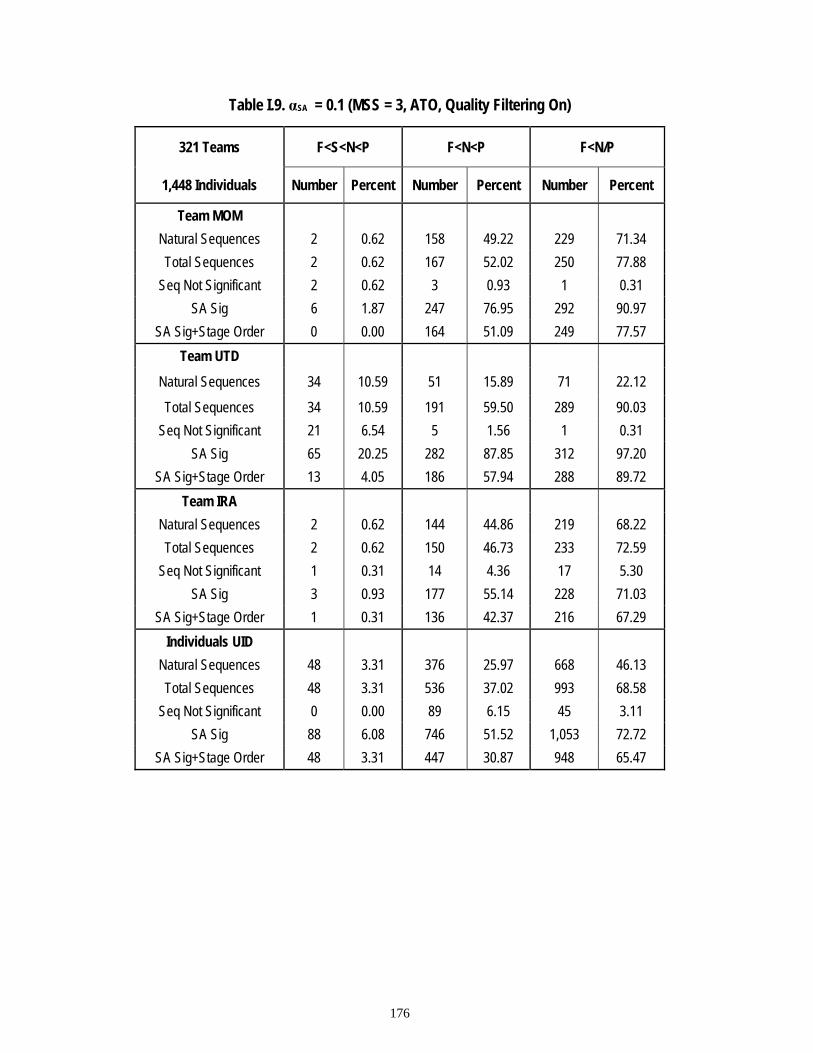
176

Table I.9. αSA = 0.1 (MSS = 3, ATO, Quality Filtering On)

321 Teams F<S<N<P F<N<P F<N/P

1,448 Individuals Number Percent Number Percent Number Percent

Team MOM Natural Sequences 2 0.62 158 49.22 229 71.34 Total Sequences 2 0.62 167 52.02 250 77.88

Seq Not Significant 2 0.62 3 0.93 1 0.31 SA Sig 6 1.87 247 76.95 292 90.97

SA Sig+Stage Order 0 0.00 164 51.09 249 77.57 Team UTD

Natural Sequences 34 10.59 51 15.89 71 22.12

Total Sequences 34 10.59 191 59.50 289 90.03 Seq Not Significant 21 6.54 5 1.56 1 0.31

SA Sig 65 20.25 282 87.85 312 97.20 SA Sig+Stage Order 13 4.05 186 57.94 288 89.72

Team IRA Natural Sequences 2 0.62 144 44.86 219 68.22 Total Sequences 2 0.62 150 46.73 233 72.59

Seq Not Significant 1 0.31 14 4.36 17 5.30 SA Sig 3 0.93 177 55.14 228 71.03

SA Sig+Stage Order 1 0.31 136 42.37 216 67.29 Individuals UID

Natural Sequences 48 3.31 376 25.97 668 46.13 Total Sequences 48 3.31 536 37.02 993 68.58

Seq Not Significant 0 0.00 89 6.15 45 3.11 SA Sig 88 6.08 746 51.52 1,053 72.72

SA Sig+Stage Order 48 3.31 447 30.87 948 65.47

177

Table I.10. αSA = 0.15 (MSS = 3, ATO, Quality Filtering On)

321 Teams F<S<N<P F<N<P F<N/P

1,448 Individuals Number Percent Number Percent Number Percent

Team MOM Natural Sequences 2 0.62 158 49.22 229 71.34 Total Sequences 2 0.62 167 52.02 250 77.88

Seq Not Significant 2 0.62 2 0.62 1 0.31 SA Sig 6 1.87 249 77.57 293 91.28

SA Sig+Stage Order 0 0.00 165 51.40 249 77.57

Team UTD

Natural Sequences 34 10.59 51 15.89 71 22.12

Total Sequences 34 10.59 191 59.50 289 90.03 Seq Not Significant 21 6.54 4 1.25 1 0.31

SA Sig 65 20.25 284 88.47 313 97.51 SA Sig+Stage Order 13 4.05 187 58.26 288 89.72

Team IRA Natural Sequences 2 0.62 144 44.86 219 68.22 Total Sequences 2 0.62 150 46.73 233 72.59

Seq Not Significant 1 0.31 9 2.80 10 3.12 SA Sig 3 0.93 193 60.12 241 75.08

SA Sig+Stage Order 1 0.31 141 43.93 223 69.47 Individuals UID

Natural Sequences 48 3.31 376 25.97 668 46.13 Total Sequences 48 3.31 536 37.02 993 68.58

Seq Not Significant 0 0.00 0 0.00 45 3.11 SA Sig 88 6.08 790 54.56 1,112 76.80

SA Sig+Stage Order 48 3.31 536 37.02 948 65.47

178

Table I.11. αSA = 0.20 (MSS = 3, ATO, Quality Filtering On)

321 Teams F<S<N<P F<N<P F<N/P

1,448 Individuals Number Percent Number Percent Number Percent

Team MOM Natural Sequences 2 0.62 158 49.22 229 71.34 Total Sequences 2 0.62 167 52.02 250 77.88

Seq Not Significant 2 0.62 2 0.62 0 0.00 SA Sig 6 1.87 249 77.57 294 91.59

SA Sig+Stage Order 0 0.00 165 51.40 250 77.88 Team UTD

Natural Sequences 34 10.59 51 15.89 71 22.12

Total Sequences 34 10.59 191 59.50 289 90.03 Seq Not Significant 21 6.54 4 1.25 0 0.00

SA Sig 65 20.25 284 88.47 314 97.82 SA Sig+Stage Order 13 4.05 187 58.26 289 90.03

Team IRA Natural Sequences 2 0.62 144 44.86 219 68.22 Total Sequences 2 0.62 150 46.73 233 72.59

Seq Not Significant 1 0.31 9 2.80 4 1.25 SA Sig 3 0.93 193 60.12 249 77.57

SA Sig+Stage Order 1 0.31 141 43.93 229 71.34 Individuals UID

Natural Sequences 48 3.31 376 25.97 668 46.13 Total Sequences 48 3.31 536 37.02 993 68.58

Seq Not Significant 0 0.00 0 0.00 37 2.56 SA Sig 88 6.08 790 54.56 1,137 78.52

SA Sig+Stage Order 48 3.31 536 37.02 956 66.02

179

Table I.12. αSA = 0.25 (MSS = 3, ATO, Quality Filtering On)

321 Teams F<S<N<P F<N<P F<N/P

1,448 Individuals Number Percent Number Percent Number Percent

Team MOM Natural Sequences 2 0.62 158 49.22 229 71.34 Total Sequences 2 0.62 167 52.02 250 77.88

Seq Not Significant 2 0.62 2 0.62 0 0.00 SA Sig 6 1.87 249 77.57 294 91.59

SA Sig+Stage Order 0 0.00 165 51.40 250 77.88 Team UTD

Natural Sequences 34 10.59 51 15.89 71 22.12

Total Sequences 34 10.59 191 59.50 289 90.03 Seq Not Significant 21 6.54 4 1.25 0 0.00

SA Sig 65 20.25 284 88.47 314 97.82 SA Sig+Stage Order 13 4.05 187 58.26 289 90.03

Team IRA Natural Sequences 2 0.62 144 44.86 219 68.22 Total Sequences 2 0.62 150 46.73 233 72.59

Seq Not Significant 1 0.31 9 2.80 4 1.25 SA Sig 3 0.93 193 60.12 249 77.57

SA Sig+Stage Order 1 0.31 141 43.93 229 71.34 Individuals UID

Natural Sequences 48 3.31 376 25.97 668 46.13 Total Sequences 48 3.31 536 37.02 993 68.58

Seq Not Significant 0 0.00 0 0.00 37 2.56 SA Sig 88 6.08 790 54.56 1,137 78.52

SA Sig+Stage Order 48 3.31 536 37.02 956 66.02

180

Appendix I.3: Non-validated Sequences Observed in Raw Data This sub-appendix looks at the non-validated (no statistical significance required) sequences generated from raw time-of-occurrence data. Table I.13 and Figure I.3 use averaged time-of-occurrence (ATO) data, which is the standard for this research project. Table I.13 shows the frequency of occurrence of every possible sequence for all three team configurations (see Chapter VI).

181

Table I.13. Raw Timing Data (Non-validated) Sequences Observed by Individuals and Teams (ATO, Quality Filtering On)

INDIV Team MOM Team UTD Team IRA INDIV Team MOM Team UTD Team IRA SEQ

Freq % Freq % Freq % Freq % SEQ

Freq % Freq % Freq % Freq %

FSNP 48 3% 2 1% 34 11% 2 1% SFN 6 0% 0 0% 0 0% 0 0% FSPN 70 5% 8 2% 37 12% 4 1% SNF 3 0% 0 0% 0 0% 0 0% FNPS 57 4% 5 2% 67 21% 3 1% SPF 3 0% 0 0% 0 0% 0 0% FNSP 35 2% 2 1% 17 5% 1 0% SFP 11 1% 0 0% 0 0% 1 0% FPSN 20 1% 1 0% 11 3% 1 0% NPF 37 3% 3 1% 1 0% 3 1% FPNS 35 2% 1 0% 14 4% 0 0% NFP 120 8% 14 4% 7 2% 23 7% SNPF 4 0% 0 0% 2 1% 0 0% NSF 2 0% 0 0% 0 0% 0 0% SNFP 5 0% 0 0% 4 1% 0 0% NFS 2 0% 0 0% 0 0% 0 0% SPFN 16 1% 0 0% 0 0% 0 0% NSP 2 0% 1 0% 0 0% 0 0% SPNF 12 1% 0 0% 0 0% 0 0% NPS 1 0% 0 0% 0 0% 0 0% SFNP 20 1% 0 0% 22 7% 0 0% PFS 5 0% 0 0% 0 0% 0 0% SFPN 40 3% 2 1% 16 5% 3 1% PSF 4 0% 0 0% 0 0% 0 0% NPFS 6 0% 0 0% 0 0% 0 0% PSN 3 0% 0 0% 0 0% 0 0% NPSF 1 0% 0 0% 0 0% 0 0% PNS 0 0% 0 0% 0 0% 0 0% NFSP 9 1% 0 0% 0 0% 0 0% PNF 27 2% 2 1% 1 0% 2 1% NFPS 16 1% 2 1% 7 2% 2 1% PFN 66 5% 3 1% 0 0% 8 2% NSPF 5 0% 0 0% 1 0% 0 0% FS 0 0% 2 1% 0 0% 2 1% NSFP 4 0% 1 0% 2 1% 0 0% FN 0 0% 3 1% 0 0% 3 1% PFSN 6 0% 0 0% 1 0% 0 0% FP 0 0% 14 4% 0 0% 20 6% PFNS 6 0% 1 0% 3 1% 0 0% SN 0 0% 0 0% 0 0% 0 0% PSNF 1 0% 0 0% 0 0% 0 0% SP 0 0% 0 0% 0 0% 1 0% PSFN 4 0% 1 0% 1 0% 0 0% SF 0 0% 0 0% 0 0% 0 0% PNSF 2 0% 0 0% 0 0% 0 0% NP 0 0% 5 2% 0 0% 5 2% PNFS 1 0% 0 0% 1 0% 0 0% NF 0 0% 1 0% 0 0% 2 1% FSN 4 0% 0 0% 0 0% 0 0% NS 0 0% 0 0% 0 0% 0 0% FNS 4 0% 0 0% 0 0% 0 0% PF 0 0% 1 0% 0 0% 0 0% FSP 28 2% 8 2% 1 0% 8 2% PS 0 0% 0 0% 0 0% 0 0% FPS 21 1% 5 2% 0 0% 2 1% PN 0 0% 1 0% 0 0% 3 1% FNP 376 26% 158 49% 51 16% 144 45% F 0 0% 1 0% 0 0% 1 0% FPN 292 20% 71 22% 20 6% 75 23% S 0 0% 1 0% 0 0% 1 0% SNP 3 0% 1 0% 0 0% 0 0% N 0 0% 0 0% 0 0% 0 0% SPN 5 0% 0 0% 0 0% 0 0% P 0 0% 0 0% 0 0% 1 0%

Figure I.3 shows the top 24 most often occurring sequences sorted from greatest to smallest and the percent of teams supporting each of the three models being studied (F<S<N<P, F<N<P, and F,N/P) for individuals and for each of the three team analysis configurations (Team MOM, Team UTD, and Team IRA). Note that Team UTD generates many more four-stage sequences than the others because it retains Storming data that are spurious or non-representative of a team’s collective experience. Because it spreads itself more thinly over more of the possible 64 sequences, it does not generate very high frequencies in any sequence. Thus keeping the anomalous data prevents

182

Team UTD from noticing the very strong following for the two Tuckman variants (F<N<P and F<N/P). Team MOM and Team IRA more clearly see a stronger following for the three-stage F<N<P model than the others. This is because they have less noise than Team UTD and more collected coherency than the individuals. Team MOM is the better of the two because, being less constrained, it sees significantly more statistically valid sequences than Team IRA.

Individual (ATO)

050

100150200250300350400

FNP

FPN

NFP

FSPN PF

NFN

PSFS

NPSF

PN NPF

FNSP

FPNS FS

PPN

FFP

SFP

SNSF

NPSP

FNNF

PSSP

NF SFP

NFSP

PFSN

NPFS

PFNS

Raw Timing Data Sequence

Num

ber o

f Cou

nts Individual ATO

0

10

20

30

40

50

FSNP FNP FPN Total

Sequence

Perc

ent o

f Ind

ividu

als

Supp

ortin

g

Team (MOM) ATO

020406080

100120140160180

FNP

FPN

NFP FP

FSPN FS

PFN

PS FPS NP PFN

NPF FN

FNSP

FSNP PN

FNF

PSSF

PN FSFP

NSFP

SN F

Raw Timing Data Sequence

Num

ber o

f Cou

nts Team (MOM) ATO

01020304050607080

FSNP FNP FPN Total

Sequence

Perc

ent o

f Tea

ms

Supp

ortin

g

Team (UTD) ATO

01020304050607080

FNPS FN

PFS

PNFS

NPSF

NP FPN

FNSP

SFPN

FPNS

FPSN

NFPS NF

PSN

FPPF

NSSN

PFNS

FP FSP

NSPF PN

FPS

FN NPF

Raw Timing Data Sequence

Num

ber o

f Cou

nts Team (UTD) ATO

05

101520253035

FSNP FNP FPN Total

Sequence

Perc

ent o

f Tea

ms

Supp

ortin

g

Team (IRA) ATO

020406080

100120140160

FNP

FPN

NFP FP FSP

PFN NP

FSPN

FNPS

SFPN FN NP

F PNFS

NP FPS

NFPS PN

F NF FSFN

SPFP

SN F P S

Raw Timing Data Sequence

Num

ber o

f Cou

nts Team (IRA) ATO

0

2040

60

80

100

FSNP FNP FPN Total

Sequence

Perc

ent o

f Tea

ms

Supp

ortin

g

Figure I.3. Sorted Raw Timing Data (Non-validated) Sequences Observed by Individuals and Teams Using Average Time-of-Occurrence (ATO) (Quality Filtering On)

183

Appendix I.4: How Results Are Affected by Combining Multiple Event Times with

Average Time-of-Occurrence (ATO) or Median Time-of-Occurrence (MTO), or First Time-of-Occurrence (FTO)

This sub-appendix provides more detail of how alternative analytical methodologies affect the final results. A more thorough assessment of using the median function will be given.

Table I.14. Median Time-of-Occurrence (MSS = 3, αSA = 0.05, Quality Filtering On)

309 Teams F<S<N<P F<N<P F<N/P

1,336 Individuals Number Percent Number Percent Number Percent

Team MOM Natural Sequences 0 0.00 138 44.66 204 66.02 Total Sequences 0 0.00 144 46.60 219 70.87

Seq Not Significant 0 0.00 9 2.91 1 0.32 SA Sig 4 1.29 214 69.26 281 90.94

SA Sig+Stage Order 0 0.00 135 43.69 218 70.55 Team UTD

Natural Sequences 33 10.68 46 14.89 67 21.68

Total Sequences 33 10.68 159 51.46 248 80.26 Seq Not Significant 21 6.80 7 2.27 1 0.32

SA Sig 64 20.71 254 82.20 303 98.06 SA Sig+Stage Order 12 3.88 152 49.19 247 79.94

Team IRA Natural Sequences 1 0.32 131 42.39 207 66.99 Total Sequences 1 0.32 136 44.01 221 71.52

Seq Not Significant 0 0.00 26 8.41 30 9.71 SA Sig 5 1.62 140 45.31 199 64.40

SA Sig+Stage Order 1 0.32 110 35.60 191 61.81 Individuals UID

Natural Sequences 32 2.40 323 24.18 583 43.64 Total Sequences 32 2.40 456 34.13 861 64.45

Seq Not Significant 0 0.00 60 4.49 77 5.76 SA Sig 87 6.51 613 45.88 959 71.78

SA Sig+Stage Order 32 2.40 396 29.64 784 58.68

184

Comparing Table I.14 (median) with Table I.3 (average) shows (see upper left hand corner of both tables) that using the median function causes 12 teams and 112 individuals to be dropped from consideration. The reasons for this (third stage of the data input quality filter) were discussed in Appendix I.1. If the median function (MTO methodology) were to be used to assess the DAU teams, one would have to determine if the third stage of the data input quality filter should be set differently (CAT = 2 instead of CAT = 3 perhaps). Beyond that glaring difference, a comparison of the two tables indicates that when the median function is used to combine multiple time-of-occurrence points on a single timeline, the results generally show significantly fewer statistically valid occurrences of F<S<N<P, F<N<P, or F<N/P models being followed by the DAU teams. The explanation is that statistical significance is harder to come by if the data are noisier. Figures I.4, I.5, and I.6 each contain two charts. The first (left most) reflects the results of using the median to combine time-of-occurrence data while the chart on the right reflects the results of using averaging to combine time-of-occurrence data. In Figure I.4, note that the standard deviation for all stages (reflecting noise levels in the data) is greater when the median is used, and that the Forming stage occurs two timeline units earlier. Figures I.5 and I.6 indicate that both the number of members on a team and the number of teams decrease when the noisier median function is used. Note that using median rather than averaging for combining time-of-occurrence data creates a larger number of smaller (three-person) teams and a much smaller number of larger (4- and 5-person) teams. Tables I.15 and I.16 show the correlation between team performance and the development model (F<S<N<P, F<N<P, or F<N/P) followed. Table I.15 gives the correlation values (probability that there is a positive correlation between the quality of a team’s products and the team development model followed) for teams that used the median rather than averaging for combining time-of-occurrence data. Table I.16 gives the same information for teams that used averaging rather than the median for combining time-of-occurrence data. The grey areas indicate relationships between the quality of a team’s products and the team development model followed that are considered to be statistically significant (probability of 0.05 or less that there is no correlation). Using the median adds enough noise to the collected data to cause Team MOM to completely miss the relationship between performance and development model followed. Only Team IRA has the robustness to take the additional noise in stride and maintain its awareness of the relationship between performance and the development model followed. Table I.17 shows why, using the MTO method, Team MOM was no longer able to discern a relationship between performance and the development model followed. In this table the MTO data are on the left and the ATO data are on the right. Clearly, using MTO methodology reduces the number of above average and average teams that observed statistically significant F<S<N<P, F<N<P, or F<N/P sequences.

185

0.00

5.00

10.00

15.00

20.00

25.00

Forming Storming Norming Performing

Tim

eline

Uni

ts

0.00

5.00

10.00

15.00

20.00

25.00

Forming Storming Norming Performing

Tim

eline

Uni

ts

Time Value Std DevTime Value Std Dev

Figure I.4. Team Average Time-of-Occurrence by Tuckman Stage

(MTO Left and ATO Right)

0

1

2

3

4

5

6

Original Responding ResearchQualified

Num

ber o

f Mem

bers

Original Responding

Num

ber o

f Mem

bers

ResearchQualified

0

1

2

3

4

5

6

Figure I.5. Average Team Sizes for Original, Responding, and Qualified Teams (MTO Left and ATO Right)

0

20

40

60

80

100

120

0 2 4 6 8 10Number of Team Members

Num

ber o

f Tea

ms

0

20

40

60

80

100

0 2 4 6 8 10Number of Team Members

Num

ber o

f Tea

ms

Research Qualified OriginalResearch Qualified Original

Figure I.6. Frequency of Team Sizes for Qualified and Original Database (MTO Left and ATO Right)

186

Table I.15. Correlation between Team Performance and MTO Team Development Model Followed for Three Analytical Team Formations and Four Performance Pairs

Above

Average Above Average

and Average Average Above Average

vs. vs. vs. vs. Team Type Model Overall

Average Below Average Below Average

Average and Below Average

F<S<N<P 0.8 0.8794 0.7616 0.8794 0.7616 F<N<P 0.3 0.4977 0.4977 0.353 0.6006 Team

MOM F<N/P 0.9 0.9273 0.7616 0.4977 0.968

F<S<N<P 0.3 0.158 0.6006 0.6006 0.353 F<N<P 0.1 0.353 0.112 #N/A 0.353 Team

UTD F<N/P 0.3 0.4977 0.4977 0.6006 0.353

F<S<N<P 0.95 0.968 0.353 #N/A 0.9856 F<N<P 0.98 0.7616 0.9856 0.9273 0.9273 Team

IRA F<N/P 0.9975 0.9948 0.9273 0.6006 0.9989

Table I.16. Correlation between Team Performance and ATO Team Development Model

Followed for Three Analytical Team Formations and Four Performance Pairs

Above Average

Above Average and Average Average Above Average

vs. vs. vs. vs. Team Type Model Overall

Average Below Average Below Average

Average and Below Average

F<S<N<P 0.95 0.9856 0.4977 #N/A 0.9856 F<N<P 0.99 0.9273 0.968 0.8794 0.9856 Team

MOM F<N/P 0.95 0.9856 0.6006 0.248 0.9856

F<S<N<P 0.8 0.7616 0.7616 0.8794 0.4977 F<N<P 0.9 0.7616 0.9273 0.7616 0.8794 Team

UTD F<N/P 0.1 0.353 0.112 #N/A 0.353

F<S<N<P 0.8 0.9273 0.353 #N/A 0.9273 F<N<P 0.95 0.6006 0.968 0.9273 0.7616 Team

IRA F<N/P 0.9995 0.9948 0.9856 0.8794 0.9995

187

Table I.17. Instructor Evaluation vs. Teams Producing Statistically Significant Sequences for Both MTO and ATO Methodologies

Figures I.7 and I.8 show the separation in time of consecutive stage means that were both successfully (Figure I.7) and unsuccessfully (Figure I.8) separated by the Kruskal-Wallis (KW) statistical test. (See Appendix L for details on how to interpret the graphs.) In both figures, MTO output is shown by the left graph while ATO output is shown by the right graph. Because the KW test is very sensitive to noise in the data (has a more difficult time differentiating between populations if the population data are noisy), these two figures clearly demonstrate the effect of increased noise levels generated by using the median rather than using averaging to combine time-of-occurrence data. From Figure I.7, one sees that MTO methodology requires two to four additional timeline units between consecutive peaks before the KW test can declare the stages to be discrete to a 95% level of confidence. From Figure I.8, one sees that MTO methodology is still failing to find discrete stages even though consecutive peaks are separated by two or more additional timeline units beyond the point where the ATO methodology begins to have trouble seeing distinct populations.

AverageMin

Min Min AverageAverage

MinAverage

Successful Separations

Tim

eline

Uni

ts

0.002.004.006.008.00

10.0012.0014.0016.0018.00

Successful Separations

Tim

eline

Uni

ts

AverageMin

Min Min AverageAverage

MinAverage

0.002.004.006.008.00

10.0012.0014.0016.0018.00

Figure I.7. MTO (Left) and ATO (Right) Successful KW Filter Stage Differentiation Terms of Timeline Units

Sequence MTO Rating Number Percent Sequence ATO Rating Number Percent

Above Average (140) 3 2.14% Above Average (145) 6 4.14%

Average (145) 0 0.00% Average (151) 0 0.00% F<S<N<P

Below Average (24) 1 4.17%

F<S<N<P

Below Average (25) 0 0.00%

Above Average (140) 101 72.14% Above Average (145) 114 78.62%

Average (145) 98 67.59% Average (151) 102 67.55% F<N<P

Below Average (24) 15 62.50%

F<N<P

Below Average (25) 13 52.00%

Above Average (140) 133 95.00% Above Average (145) 138 95.17%

Average (145) 128 88.28% Average (151) 131 86.75% F<N/P

Below Average (24) 20 83.33%

F<N/P

Below Average (25) 21 84.00%

188

Failed Separations

Tim

eline

Uni

ts

AverageMax

Max Max AverageAverage

MaxAverage

0.00

5.00

10.00

15.00

20.00

25.00

30.00

Failed Separations

Tim

eline

Uni

ts

AverageMax

Max Max AverageAverage

MaxAverage

0.00

5.00

10.00

15.00

20.00

25.00

30.00

Figure I.8. MTO (Left) and ATO (Right) Failed KW Filter Stage Differentiation Terms of Timeline Units

Figures I.9 and I.10 show MTO and ATO Distribution of Tuckman stages occurring at specific locations on the timeline for the 321 DAU teams. These two graphs provide the most striking evidence of the difficulties generated by using MTO methodology. Because of an increase in ties and the erratic fluctuations produced by using MTO methodology, the Norming and Performing peaks become indistinguishable and both fall at the exact center of the timeline. It is no wonder that the results of this research change dramatically when the median function is used.

0102030405060708090

100

0 2 4 6 8 10 12 14 16 18 20 22 24 26 28 30 32 34 36 38 40Timeline Units

Num

ber o

f Occ

urre

nces

Forming Storming Norming Performing

Figure I.9. MTO Distribution of Tuckman Stages Occurring at Specific Locations on the Timeline

189

0369

1215182124273033

0 2 4 6 8 10 12 14 16 18 20 22 24 26 28 30 32 34 36 38 40Timeline Units

Num

ber o

f Occ

urre

nces

Forming Storming Norming Performing

Figure I.10. ATO Distribution of Tuckman Stages Occurring at Specific Locations on the Timeline

Finally, Figures I.11 and I.12 show the raw timing sequences generated under the MTO and FTO methodology. These should be compared to Figure I.3, which presents similar data for the ATO methodology. It can be seen that when utilizing the ATO methodology, the data indicate more occurrence of the F<N<P sequence than does either the MTO or the FTO methodologies. The FTO methodology finds less F<N<P sequences than the MTO methodology. This is as expected. Though the FTO does not have the problem with ties that the MTO has, it has an even greater problem with accurately defining stage locations. The bottom line here is that one’s choice of analysis methodology may have a significant effect upon the results. Thus, it is important to study all alternative methodologies and select the ones that most accurately depict the signal (information reflecting the experiences of DAU teams) within the collected data.

190

Individual (MTO)

050

100150200250300350

FNP

FPN

NFP

FSPN PF

NFN

PSFN

SPSF

PN FSP

FSNP PN

FNP

FFP

NS FPS FN

FPSN

SFNP

SPFN FN

SNF

PSSP

NF FSN

SFP

NFSP

Raw Timing Data Sequence

Num

ber o

f Cou

nts

Individual MTO

0

10

20

30

40

50

FSNP FNP FPN TotalSequence

Perc

ent o

f Ind

ividu

als

Supp

ortin

g

Team (MOM) MTO

020406080

100120140160

FNP

FPN FN FP FSP

FSPN NF

PFN

PS FPS F NF NP PFN FS PN NPF

FNSP PF NS

PSP

FN SFP

Raw Timing Data Sequence

Num

ber o

f Cou

nts Team (MOM) MTO

01020304050607080

FSNP FNP FPN TotalSequence

Perc

ent o

f Tea

ms

Supp

ortin

gTeam (UTD) MTO

05

101520253035404550

FNP

FNPS

FSPN

FSNP

FNSP FP

NFP

NSSF

NPSF

PN FSP

FNS

FPSN FS

N FNNF

PSSN

FPSP

FN FPNS

PF SFN

FPS

Raw Timing Data Sequence

Num

ber o

f Cou

nts Team (UTD) MTO

05

101520253035

FSNP FNP FPN Total

Sequence

Perc

ent o

f Tea

ms

Supp

ortin

g

Team (IRA) MTO

020406080

100120140

FNP

FPN

NFP FP FSP

PFN

FSPN FN NP

F PN PNF NP FPS NF

FNPS

SFPN FS

FNSP F P

FSNP

FPSN S

SFP

Raw Timing Data Sequence

Num

ber o

f Cou

nts Team (IRA) MTO

0

2040

6080

100

FSNP FNP FPN Total

Sequence

Perc

ent o

f Tea

ms

Supp

ortin

g

Figure I.11. Sorted Raw Timing Data (Non-validated) Sequences Observed by Individuals and Teams Using Median Time-of-Occurrence (MTO)

191

Individual (FTO)

050

100150200250300350

FNP

FPN

NFP

PFN FP

FNPS

FSPN

FPNS F

FPSN NP

F FN FPS

PNF

FSP

SFPN

FSNP

FNSP

SFNP FS

NSP

FNNF

PS NFSP

NF

Raw Timing Data Sequence

Num

ber o

f Cou

nts

Individual FTO

05

1015202530354045

FSNP FNP FPN Total

Sequence

Perc

ent o

f Ind

ividu

als

Supp

ortin

g

Team (MOM) FTO

020406080

100120140

FNP

FPN

NFP FP

PFN

FSP

N FN FPS

NP

FFS

PFN

PS

NP

FSN

PFP

NS

SFP

NS

FPFP

SN

PN

FP

NS

NP FS

Raw Timing Data Sequence

Num

ber o

f Cou

nts Team (MOM) FTO

010203040506070

FSNP FNP FPN Total

Sequence

Perc

ent o

f Tea

ms

Supp

ortin

gTeam (UTD) FTO

0102030405060

FNPS FN

PFP

NSFS

PNFS

NP FPN

SFPN

SFNP

FPSN

FNSP NF

PSP

FNNF

PS PFN

SNPF

PFNS

SNFP

NSFP

PNFS FP

SFS

N

Raw Timing Data Sequence

Num

ber o

f Cou

nts Team (UTD) FTO

05

101520253035

FSNP FNP FPN Total

Sequence

Perc

ent o

f Tea

ms

Supp

ortin

g

Team (IRA) (FTO)

020406080

100120140

FNP

FPN

NFP FP PFN FN NPF

FSPN FP

SPN

FFS

PSF

P FSFN

PSSF

PNFP

SNSP

FNFP

NSNF

SP FNP

FSSF

NP PNFS

NP

Raw Timing Data Sequence

Num

ber o

f Cou

nts Team (IRA) FTO

010203040506070

FSNP FNP FPN Total

Sequence

Perc

ent o

f Tea

ms

Supp

ortin

g

Figure I.12. Sorted Raw Timing Data (Non-validated) Sequences Observed by Individuals and Teams Using First Time-of-Occurrence (FTO)

192

Appendix I.5: Results with and without Input Data Quality Filtering Table I.18 shows the results of this research under the condition of no input data quality filtering. Notice that 368 teams and 1,773 individuals are now being considered. This means that 47 teams and 325 individuals that had been discarded as unsuitable have now been returned to the research database.

Table I.18. Quality Filtering Off (MSS = 3, αSA = 0.05, ATO)

368 Teams F<S<N<P F<N<P F<N/P

1,773 Individuals Number Percent Number Percent Number Percent

Team MOM Natural Sequences 3 0.82 171 46.47 255 69.29 Total Sequences 3 0.82 180 48.91 275 74.73

Seq Not Significant 3 0.82 11 2.99 2 0.54 SA Sig 6 1.63 248 67.39 312 84.78

SA Sig+Stage Order 0 0.00 169 45.92 273 74.18 Team UTD

Natural Sequences 36 9.78 57 15.49 85 23.10 Total Sequences 36 9.78 215 58.42 327 88.86

Seq Not Significant 24 6.52 13 3.53 2 0.54 SA Sig 65 17.66 295 80.16 349 94.84

SA Sig+Stage Order 12 3.26 202 54.89 325 88.32 Team IRA

Natural Sequences 1 0.27 154 41.85 235 63.86 Total Sequences 1 0.27 161 43.75 250 67.93

Seq Not Significant 1 0.27 46 12.50 33 8.97 SA Sig 1 0.27 147 39.95 223 60.60

SA Sig+Stage Order 0 0.00 115 31.25 217 58.97 Individuals UID

Natural Sequences 49 2.76 380 21.43 680 38.35 Total Sequences 49 2.76 543 30.63 1,009 56.91

Seq Not Significant 0 0.00 107 6.03 104 5.87 SA Sig 89 5.02 647 36.49 1,029 58.04

SA Sig+Stage Order 49 2.76 436 24.59 905 51.04 Comparing this table with Table I.3 one can see how the results have degenerated in all categories now that erroneous and misleading data had been reinstated. A lower percentage of

193

statistically significant sequences are reported for all team types and all developmental models. Clearly, filtering out bad data is advantageous to the final results. Figure I.13 shows the raw timing sequence data under the condition of no input data quality filtering. Comparing this to Figure I.3 corroborates the results of Table I.18. Fewer raw F<N<P and F<N/P sequences were formed due to the influence of erroneous data.

194

Individual (ATO)

050

100150200250300350400

FNP

FPN

NFP

FSPN PF

NFN

PS FPFS

NPSF

PN NPF

FNSP

FPNS PN

FFS

P F FN FPS P

FPSN

SFNP NP PF

SPFN

NFPS

Raw Timing Data Sequence

Num

ber o

f Cou

nts

Individual ATO

0

10

20

30

40

50

FSNP FNP FPN TotalSequence

Perc

ent o

f Ind

ividu

als

Supp

ortin

g

Team (MOM) ATO

020406080

100120140160180

FNP

FPN FP NFP

FSPN FS

P NPFN

PS FPS

PFN

NPF

FSNP PN

F FS F PN P FNFN

SPSF

PN SP

Raw Timing Data Sequence

Num

ber o

f Cou

nts

Team (MOM) ATO

01020304050607080

FSNP FNP FPN TotalSequence

Perc

ent o

f Tea

ms

Supp

ortin

g

Team (UTD) ATO

01020304050607080

FNPS FN

PFS

NPFS

PN FPN

SFNP

FNSP

SFPN

FPNS

FPSN

NFPS NF

PSN

FP PNF

PFNS

PSFN NP

FPF

SNNP

FSSN

PFNS

FP

Raw Timing Data Sequence

Num

ber o

f Cou

nts

Team (UTD) ATO

05

101520253035

FSNP FNP FPN TotalSequence

Perc

ent o

f Tea

ms

Supp

ortin

g

Team (IRA) ATO

020406080

100120140160180

FNP

FPN FP NFP NP PFN PN P

FSP

FNPS PN

FSF

PNFS

PN FN FS FFP

S SP PF NPF

FSNP

NFPS NF

FNSP

Raw Timing Data Sequence

Num

ber o

f Cou

nts

Team (IRA) ATO

0

2040

6080

100

FSNP FNP FPN Total

Sequence

Perc

ent o

f Tea

ms

Supp

ortin

g

Figure I.13. Sorted Raw Timing Data (Non-validated) Sequences Observed by Individuals and Teams Using Average Time-of-Occurrence (ATO) (Quality Filtering Off)

195

APPENDIX J

SEQUENCE ANALYSIS

Appendix J.1: F<S<N<P Sequence Analysis Appendix J.2: F<N<P Sequence Analysis Appendix J.3: F<N/P Sequence Analysis Appendix J.4: MSS Evaluated

196

197

Appendix J.1: F<S<N<P Sequence Analysis A. Introduction In Appendix L, the discussion of combining individual data into team data breaks the analysis process into two separate parts. Part 1 calculations produce a single time-of-occurrence per question per individual, while Part 2 calculations combine the individual Part 1 data to represent a collective team experience (see Appendix L.2). The Group Process Questionnaire (GPQ) contains three Forming questions, four Storming questions, four Norming questions, and four Performing questions. Each question asks if the team member observed a particular Tuckman event (Forming, Storming, Norming, or Performing) occurring within his/her group; and if so (question answered “YES”), then when did the event occur. Thus each “YES” answer comes with time-of-occurrence data marked on a 50-unit timeline. Part 1 calculations combine this timeline data into a single time-of-occurrence datum for each question answered “YES” by each individual. Let F1 represent the time-of-occurrence of the Forming event described by the first Forming question. Likewise, N3 represents the time-of-occurrence associated with the third Norming question, and so on. It is convenient to use a subscript to designate the times-of-occurrence associated with each of the 15 Tuckman questions. Let Fi (where i can have the values 1, 2, 3) represent the time-of-occurrence of the Forming events described by the three Forming questions. Likewise let Sm represent the time-of-occurrence of the Storming events described by the four Storming questions; let Nj represent the time-of-occurrence of the Norming events described by the four Norming questions; and let Pk represent the time-of-occurrence of the Performing events described by the four Performing questions. Here, m, j, and k each, independently, may take on the values 1, 2, 3, 4. There are 192 unique possible Tuckman sequences as shown in Figure J.1 below.

1 2 3

1 2 3 4

1 2 3 4

1 2 3 4

3 Forming

4

4 Norming

4 Performing

1 2 311 22 33

1 2 3 411 22 33 44

1 2 3 411 22 33 44

1 2 3 411 22 33 4

F F F

S S S S

N N N N

P P P P4

3 Forming

Storming

4

4 Performing

Figure J.1. Fifteen Questions Produce 192 Tuckman Sequences

Notice: 15 Questions can produce as many as 15 times-of-occurrence data points (if all questions are answered “YES”). If all Forming events Fi (i.e., F1, F2, and F3) occurred before all Storming events Sm, and all Storming events occurred before all Norming events Nj, and all Norming events occurred before all Performing events Pk, then there can be as many as 3 x 4 x 4 x 4 = 192 unique Tuckman sequences generated.

198

For example: If I = 1, m = 3, j = 2, and k = 4, the sequence F1<S3<N2<P4 is defined, which is one of the 192 possible sequences, wherein the time-of-occurrence of the first Forming question (F1) is less than the time-of-occurrence of the third Storming question (S3), which in turn has a time-of-occurrence that is less than the second Norming question (N2), which in turn has a time-of-occurrence that is less than the fourth Performing question (P4). F1<S2<N4<P3 is another one of the 192 possible sequences and F3<S2<N3<P2 is yet another. A time-of-occurrence associated with each of the 15 questions enables the calculation of how many of the 192 possible Tuckman sequences (Fi<Sm<Nj<Pk) were experienced by that individual or team. This number divided by 192 and multiplied by 100 gives the percent of all possible Tuckman sequences that the individual or team experienced. This percentage is defined as their Tuckman score or FSNP-score. B. Methodology for Generating an FSNP-Score The Sequence Analysis (SA) logical algorithm is shown in Figure J.2 below. This figure shows the three Forming questions (F1, F2, and F3 across the top of each of the four sequence identification tables) being analyzed relative to the four Storming questions (S1, S2, S3, and S4—one of the four sequence identification tables is dedicated to each Storming question) and all of the Norming and Performing questions (N1, N2, N3, N4 and P1, P2, P3, P4 are arrayed in the first column of each of the four sequence identification tables). The point is to determine the order in which the four Tuckman event-stages (F, S, N, and P) occur as given by the timeline data associated with each question (see top left table of Figure J.2). Sequence generation results are enumerated in the four sequence identification tables by placing a 1 if the sequence indicated by each cell is followed and a 0 if it is not. For example, in the data upon which this sample is based the sequence F1<S1<N1<P1 did occur since 3<7<23<37. Thus, a 1 is placed in the appropriate cell (Storming 1 table, first column of numbers, first row of numbers). Likewise, since the data did not support the sequence F2<S2<N1<P2, a zero is placed in the Storming 2 table, second column of numbers, second row of numbers. The five tables shown in Figure J.2 reside in an Excel spreadsheet. A logical conditional test was generated in Excel that places 1s or 0s in the four sequence identification tables based upon the given time-of-occurrence data. Each of the four sequence identification tables could potentially produce as many as 48 ones for a total of 192 total points if the Tuckman model is followed 100% of the time by that individual or team (all ones and no zeros). The FSNP-Score is the percentage of Tuckman sequences that are generated by the answers to the 15 Tuckman questions. These scores can vary between 0 (if no Tuckman sequences are generated by the timing data) and 100 (if all 192 Tuckman sequences are generated by the timing data). Sums are shown at the bottom of each column. For example, the first column contains 9 ones.

199

Figure J.2. Sequence Analysis Logical Algorithm (Tuckman Model) In the example shown in Figure J.2, there are a total of 90 ones contained within the four sequence identification tables. In other words, 90 Tuckman sequences were generated by the 15 timing scores shown in the top left table.

Question Time-of-Occurrence

F1 3 F2 10 F3 5 S1 7 S2 15 S3 18 S4 22 N1 23 N2 20 N3 35 N4 27 P1 37 P2 21 P3 41 P4 12

Storming 2 F1 < F2 < F3 < S2< N1<

P1 1 1 1 P2 0 0 0 P3 1 1 1 P4 0 0 0

N2< P1 1 1 1 P2 1 1 1 P3 1 1 1 P4 0 0 0

N3< P1 1 1 1 P2 0 0 0 P3 1 1 1 P4 0 0 0

N4< P1 1 1 1 P2 0 0 0 P3 1 1 1 P4 0 0 0

9 9 9

Storming 1 F1 < F2 < F3 < S1<

N1< P1 1 0 1 P2 0 0 0 P3 1 0 1 P4 0 0 0

N2< P1 1 0 1 P2 1 0 1 P3 1 0 1 P4 0 0 0

N3< P1 1 0 1 P2 0 0 0 P3 1 0 1 P4 0 0 0

N4< P1 1 0 1 P2 0 0 0 P3 1 0 1 P4 0 0 0

9 0 9

Storming 3 F1 < F2 < F3 < S3<

N1< P1 1 1 1 P2 0 0 0 P3 1 1 1 P4 0 0 0

N2< P1 1 1 1 P2 1 1 1 P3 1 1 1 P4 0 0 0

N3< P1 1 1 1 P2 0 0 0 P3 1 1 1 P4 0 0 0

N4< P1 1 1 1 P2 0 0 0 P3 1 1 1 P4 0 0 0

9 9 9

Storming 4 F1 < F2 < F3 < S4<

N1< P1 1 1 1 P2 0 0 0 P3 1 1 1 P4 0 0 0

N2< P1 0 0 0 P2 0 0 0 P3 0 0 0 P4 0 0 0

N3< P1 1 1 1 P2 0 0 0 P3 1 1 1 P4 0 0 0

N4< P1 1 1 1 P2 0 0 0 P3 1 1 1 P4 0 0 0

6 6 6

200

Thus, the FSNP-score is: 875.46192

90100 =×

In Figure J.3 the exact same set of time-of-occurrence data is being analyzed, but now a three timeline unit minimum stage separation (MSS = 3) between consecutive stages has been enforced. In other words, event-stage means must be separated by at least three timeline units before they can be considered as distinct stages. For example, in Figure J.2 it was required that F1<S1<N1<P1 to generate a one in the proper cell of the sequence identification tables (indicating that the sequence had been observed). Now, in Figure J.3 it is required, not only that F1<S1, but also that F1 ≤ (S1 - 3). The criterion for the Tuckman sequence now becomes:

Fi ≤ (Sm - 3) , Sm ≤ (Nj - 3) , and Nj ≤ (Pk - 3).

Three timeline units between stage means was selected as the Minimum Stage Separation (MSS = 3) to ensure a 95% confidence that consecutive stages were separate and discrete. See Appendix N to understand why three timeline units were chosen as the optimal value of MSS. Also, Appendix J.4 explores how the choice of MSS affects the final results by raising and lowering validation thresholds. In the Figure J.3 example, there are a total of 52 ones contained within the four sequence identification tables. In other words, with MSS = 3, only 52 Tuckman sequences were generated by the same 15 timing scores used in Figure J.2 (the top left table in both figures). The FSNP-score for this example is:

08.27192

52100 =×

201

Figure J.3. Sequence Analysis Logical Algorithm (Tuckman Model) with MSS = 3

Storming 1 F1 < F2 < F3 < S1<

N1< P1 1 0 0 P2 0 0 0 P3 1 0 0 P4 0 0 0

N2< P1 1 0 0 P2 0 0 0 P3 1 0 0 P4 0 0 0

N3< P1 0 0 0 P2 0 0 0 P3 1 0 0 P4 0 0 0

N4< P1 1 0 0 P2 0 0 0 P3 1 0 0 P4 0 0 0

7 0 0

Storming 2 F1 < F2 < F3 < S2< N1<

P1 1 1 1 P2 0 0 0 P3 1 1 1 P4 0 0 0

N2< P1 1 1 1 P2 0 0 0 P3 1 1 1 P4 0 0 0

N3< P1 0 0 0 P2 0 0 0 P3 1 1 1 P4 0 0 0

N4< P1 1 1 1 P2 0 0 0 P3 1 1 1 P4 0 0 0

7 7 7

Question Time-of-Occurrence

F1 3 F2 10 F3 5 S1 7 S2 15 S3 18 S4 22 N1 23 N2 20 N3 35 N4 27 P1 37 P2 21 P3 41 P4 12

Storming 3 F1 < F2 < F3 < S3<

N1< P1 1 1 1 P2 0 0 0 P3 1 1 1 P4 0 0 0

N2< P1 0 0 0 P2 0 0 0 P3 0 0 0 P4 0 0 0

N3< P1 0 0 0 P2 0 0 0 P3 1 1 1 P4 0 0 0

N4< P1 1 1 1 P2 0 0 0 P3 1 1 1 P4 0 0 0

5 5 5

Storming 4 F1 < F2 < F3 < S4<

N1< P1 0 0 0 P2 0 0 0 P3 0 0 0 P4 0 0 0

N2< P1 0 0 0 P2 0 0 0 P3 0 0 0 P4 0 0 0

N3< P1 0 0 0 P2 0 0 0 P3 1 1 1 P4 0 0 0

N4< P1 1 1 1 P2 0 0 0 P3 1 1 1 P4 0 0 0

3 3 3

202

C. Statistical Significance of FSNP-Scores Once an FSNP-Score value (between 0-100) is calculated, the significance of the score must be determined. To define statistical significance, the distribution of the Tuckman sequence algorithm must be developed. To create the distribution of the SAF<S<N<P algorithm, 102,000 questionnaires were simulated using random inputs. The output of these simulated questionnaires (representing completely random timeline data for each random “YES” answer) with a minimum stage separation of 3 timeline units (MSS = 3) was run through the Tuckman SA algorithm, and the resulting 102,000 FSNP-Scores were sorted into bins between 1 and 100. The distribution of the output of these questionnaires was then plotted and is shown in Figure J.4 along with a curve fit to the closest normal distribution (at two ordinate scales).

0100002000030000400005000060000700008000090000

100000

0 0.2 0.4 0.6 0.8 1 1.2 1.4 1.6 1.8 2FSNP-Score

Num

ber o

f Occ

urre

nces

F<S<N<P Distribution Normal Distribution

0200400600800

100012001400160018002000

0 0.2 0.4 0.6 0.8 1 1.2 1.4 1.6 1.8 2FSNP-Score

Num

ber o

f Occ

urre

nces

F<S<N<P Distribution Normal Distribution

Figure J.4. Random Distribution Curve—F<S<N<P Sequence Analysis

Notice the fluctuations in the data. These are real and do NOT represent too few samples. This effect appears to be an artifact of the logical algorithm and is due to the rather limited ways (different combinations of input data) there are to produce a given specific score value. Some values (usually following patterns) are impossible to achieve and therefore have zero values. The fluctuations seen here at the lower score values are artifacts of these zero values that have been washed out by multiple zeros being spanned by the size of the bins. In other words, this is a logical algorithm function and not a continuous function. The distribution was used to generate a cumulative probability curve, which is shown in Figure J.5. A probability is generated from each point on the distribution curve by dividing the area under the distribution curve to the right of the point by the total area under the distribution curve. Note that for the given data, an FSNP-score must be equal to or greater than 0.098 to achieve a 95 percentile level of confidence that it was not produced by random inputs. More explicitly:

αSA = P(0.098) = 0.05

203

00.05

0.10.15

0.20.25

0.30.35

0.40.45

0.50.55

0.60.65

0.70.75

0.80.85

0.90.95

1

0 0.1 0.2 0.3 0.4 0.5 0.6 0.7 0.8 0.9 1 1.1 1.2 1.3 1.4 1.5FSNP-Score

Prob

abilit

y

Figure J.5. Cumulative Probability Model Tuckman Sequence Analysis In other words, an FSNP-score of ≥ 0.098 has a probability of ≤ 0.05 of being produced from an input data set (single questionnaire) that has random answers (“YES,” “NO,” or “UNCERTAIN” for each of the 15 questions and random values (between 0 and 50) for the time-of-occurrence of the Tuckman events associated with each random “YES” answer. Thus, the probability curve is used to determine what FSNP-score represents the αSA = 0.05 level of statistical significance (95% level of confidence). An FSNP-score that has ≤ .05 probability of being generated by random time-of-occurrence data is defined as a significant score. Any set of timing data (defined by the 15 time-of-occurrence data points generated by each questionnaire) that produces a significant FSNP-score is considered to represent a statistically valid sequence. The occurrence of teams following the Tuckman model reported by this research is based only upon those teams that produce Tuckman stage sequences with scores that are statistically significant. D. Variations of the Tuckman Model In addition to determining if an individual or team is following the Tuckman model at or beyond the 95% level of confidence, this research looked at what other possible sequences of Tuckman events were being experienced by the teams (e.g., Forming, Norming, Performing or Forming, Norming, Storming, Performing, etc.). Raw time-of-occurrence data were used to determine what other models should be evaluated. Sequences were defined by ordering the average time-of-occurrence of each stage from smallest time-of-occurrence to largest time-of-occurrence. There are 64 possible combinations of alternative sequences of the Tuckman stages. For each individual and for each team, an assessment was performed to determine which of these 64

204

sequences were being followed. A distribution of the frequency of occurrence of each possible timing sequence was then graphed (see Figures J.6 and J.7) to determine which timing sequences occur most often. The most prevalent sequence being followed by both DAU teams and individuals is F<N<P. The next most prevalent sequence being followed is F<P<N.

0

50

100

150

200

250

300

350

400

FSNP

FSPN

FNPS

FNSP

FPSN

FPNS

SNPF

SNFP

SPFN

SPNF

SFNP

SFPN

NPFS

NPSF

NFSP

NFPS

NSPF

NSFP

PFSN

PFNS

PSNF

PSFN

PNSF

PNFS FS

NFN

SFS

PFP

SFN

PFP

NSN

PSP

NSF

NSN

FSP

FSF

PNP

FNF

PNS

FNF

SNS

PNP

SPF

SPS

FPS

NPN

SPN

FPF

N FS FN FP SN SP SF NP NF NS PF PS PN F S N P

All Possible Sequences of Tuckman Stages

Num

ber o

f Occ

urre

nces

forI

ndivi

duals

Figure J.6. Distribution of Alternative Arrangements of Tuckman Stages for Individuals

0

20

40

60

80

100

120

140

160

FSNP

FSPN

FNPS

FNSP

FPSN

FPNS

SNPF

SNFP

SPFN

SPNF

SFNP

SFPN

NPFS

NPSF

NFSP

NFPS

NSPF

NSFP

PFSN

PFNS

PSNF

PSFN

PNSF

PNFS FS

NFN

SFS

PFP

SFN

PFP

NSN

PSP

NSF

NSN

FSP

FSF

PNP

FNF

PNS

FNF

SNS

PNP

SPF

SPS

FPS

NPN

SPN

FPF

N FS FN FP SN SP SF NP NF NS PF PS PN F S N P

All Possible Sequences Of Tuckman Stages

Num

ber o

f Occ

urre

nces

for T

eam

(MO

M)

Figure J.7. Distribution of Alternative Arrangements of Tuckman Stages for Team MOM In the exact same way that the SA logical algorithm SAF<S<N<P was developed for the Tuckman sequence, a SA algorithm SAF<N<P was created and applied to the sequences Fi < Nj < Pk. Likewise a SA algorithm SAF<N/P was created and applied to the sequences Fi < (Nj and Pk). (See Appendix J.2 and J.3 for more detail on F<N<P and F<N/P distributions and SA calculations.)

205

E. Assessment of Three Potential Models of Team Dynamics In order to assess a sensitivity analysis of the parameters αSA and MSS, a complete set of distributions and probability curves for the values of αSA = 0.1, 0.15, 0.2, 0.25, 0.5 and MSS = 0.01, 1, 3, 5, 7, 9 were developed (see Appendix I for results) for the following three sequences:

1) The four-stage Tuckman sequence F<S<N<P 2) The three-stage F<N<P sequence and 3) The two-stage F<N/P.

The last, F<N/P, means that Forming comes before both Norming and Performing—whether Norming comes before Performing or Performing occurs before Norming is irrelevant. In other words, F<N/P represents both F<N<P and F<P<N combined together as one two-stage sequence F<N/P. For any given value of αSA and for any given value of MSS, the lowest FSNP-score, FNP-Score, or FN/P-Score that is statistically significant for each of the three models being considered can be specified. A need for statistical rigor supported the choice of αSA = 0.05 and MSS = 3. When the collected team data produce a significant score result for any of the three models, the result has successfully passed through the SA algorithm. The output of the SA algorithm is an enumeration of the number of statistically significant results that occur for each of the three sequence models being studied. In Appendix J.2, a very similar discourse to the above, but focused on the F<N<P model instead of the F<S<N<P model is provided. In Appendix J.3, a very similar discourse to the above, but focused on the F<N/P model is provided. In Appendix J.4, variations of MSS are discussed.

206

Appendix J.2: F<N<P Sequence Analysis The exact same set of time-of-occurrence data that was analyzed in Appendix J.1 is shown in Figure J.8, including a three-timeline unit minimum stage separation (MSS = 3) between consecutive stages. In other words, the requirement that stages must be separated by at least three timeline units before they can be considered as distinct stages is imposed. The general criteria for the F<N<P sequence is: F ≤ (N - 3), N≤ (P - 3). If all Fi are less than all Nj - 3 are less than all Pk - 3, then as many as 48 sequences can be generated from the 15 Tuckman questions.

Figure J.8. Sequence Analysis Logical Algorithm (F<N<P Model) with MSS = 3 In Figure J.8, there are a total of 21 ones contained within the single sequence identification table. In other words, with MSS = 3, 21 Fi ≤ Nj-3 ≤ Pk-3 sequences were generated by the same 15 timing scores used in Appendix J.1. F<N<P will be referred to as “Tuckman Variant-1” or F<N<P. The FNP-Score for this example is:

75.4348

21100 =×

Once an FNP-Score value (between 0-100) is calculated, the significance of the score must be determined. To achieve this, the distribution of the F<N<P sequence algorithm must be created. To derive the distribution curve of this algorithm, 102,000 questionnaires were simulated using random inputs. The output of these simulated questionnaires (representing

Question Time-of-

Occurrence

F1 3 F2 10 F3 5 S1 7 S2 15 S3 18 S4 22 N1 23 N2 20 N3 35 N4 27 P1 37 P2 21 P3 41 P4 12

F1 < F2 < F3 <

N1< P1 1 1 1 P2 0 0 0 P3 1 1 1 P4 0 0 0

N2< P1 1 1 1 P2 0 0 0 P3 1 1 1 P4 0 0 0

N3< P1 0 0 0 P2 0 0 0 P3 1 1 1 P4 0 0 0

N4< P1 1 1 1 P2 0 0 0 P3 1 1 1 P4 0 0 0

7 7 7

207

completely random question answers and timeline data) was run through the F<N<P SA algorithm (SAF<N<P), and the resulting 102,000 FNP-Scores were sorted into bins between 1 and 100. The distribution of the output of these questionnaires was then plotted and is shown in Figure J.9 along with a curve fit to the closest normal distribution (at two different ordinate scales). It is seen that these data have nothing in common with a normal distribution. Once again, notice the fluctuations in the data. These are real and do NOT represent too few samples. This effect appears to be an artifact of the logical algorithm and is due to the rather limited ways (different combinations of input data) there are to produce a given specific score value. Some values (usually following patterns) are impossible to achieve and therefore have zero values. The fluctuations seen here at the lower score values are artifacts of these zero values that have been washed out by multiple zeros being spanned by the size of the bins. In other words, this is a logical algorithm function and not a continuous function.

09000

180002700036000450005400063000720008100090000

0 0.5 1 1.5 2 2.5 3 3.5 4 4.5 5 5.5 6 6.5 7 7.5 8FNP-Score

Num

bero

f Occ

urre

nces

F<N<P Distribution Normal Distribution

0100020003000400050006000700080009000

10000

0 0.5 1 1.5 2 2.5 3 3.5 4 4.5 5 5.5 6 6.5 7 7.5 8FNP-Score

Num

ber o

f Occ

urre

nces

F<N<P Distribution Normal Distribution

Figure J.9. Random Distribution Curve—F<N<P Sequence Analysis The distribution was used to generate a cumulative probability curve, which is shown in Figure J.10. A probability is generated from each point on the distribution curve by dividing the area under the distribution curve to the right of the point by the total area under the distribution curve. Note that, for the given data, an FNP-Score must be equal to or greater than 4.251 to achieve a 95% level of confidence that it was not produced by random inputs. More explicitly:

αSA = P(4.251) = 0.05

208

00.050.1

0.150.2

0.250.3

0.350.4

0.450.5

0.550.6

0.650.7

0.750.8

0.850.9

0.951

0 0.5 1 1.5 2 2.5 3 3.5 4 4.5 5 5.5 6 6.5 7 7.5 8

FNP-Score

Prob

abilit

y

Figure J.10. Cumulative Probability Model F<N<P Sequence Analysis

In other words, an FNP-Score of 4.251or greater has a probability of ≤ 0.05 of being produced from an input data set (single questionnaire) that has random answers (“YES,” “NO,” or “UNCERTAIN” for each of the 15 questions) and random values (between 0 and 50) for the time-of-occurrence of the Tuckman events associated with each random “YES” answer. Thus, the probability curve is used to determine what FNP-Score represents the αSA = 0.05 level of statistical confidence (95% level of significance). An FNP-Score that has ≤ 0.05 probability of being generated by random time-of-occurrence data is defined as a significant score. Any set of timing data (defined by the 15 time-of-occurrence data points produced by each questionnaire) that produce a significant FNP-Score is considered to represent a statistically valid F<N<P sequence. F<N<P model occurrence reported by this research is based only upon those teams that produce F<N<P stage sequences with scores that are statistically significant. Other levels of confidence (αSA = 0.1, 0.15, 0.2, 0.25, 0.5) and various minimum stage separations (0, 1, 3, 5, 7, and 9) were evaluated (see Appendix I) during the sensitivity analysis of αSA and MSS. Distribution and probability curves were generated for each combination of parameters so that for any given αSA and any given MSS, the lowest FNP-Score that was statistically significant could be specified.

209

Appendix J.3: F<N/P Sequence Analysis In Figure J.11, the same set of time-of-occurrence data that was analyzed in Appendix J.1 is shown, including a three-timeline unit minimum stage separation (MSS = 3) between consecutive stages. In other words, the same requirement that stages must be separated by at least three timeline units before they can be considered as distinct stages is imposed. The general criteria for the F<N/P sequence is: F ≤ (N - 3), F≤ (P - 3). If all Fi are less than all Nj - 3 and all Fi are less than all Pk - 3, then as many as 48 sequences can be generated from the 15 Tuckman questions. Since F<N<P and F<P<N are mutually exclusive (a given sequence cannot be both F<N<P and F<P<N), the results of each are combined to get the F<N/P sequence. In those exceptional cases where Nj = Pk, care must be taken not to double count.

Figure J.11. Sequence Analysis Logical Algorithm (F<N/P Model) with MSS = 3

In the F<N<P table of Figure J.11, if Fi < Nj - 3 ≤ Pk - 3, then place a one in the appropriate cell, otherwise place a zero; whereas in the F<P<N table, if Fi < Pk- 3 < Nj - 3 then place a one in the appropriate cell, otherwise place a zero. This avoids double counting when Nj = Pk. In Figure J.11, there are a total of forty-four ones contained within the single sequence identification table. In other words, with MSS = 3, forty-four F<N/P sequences were generated by the same 15 timing scores used in Appendix J.1. F<N/P will be referred to as “Tuckman Variant 2” or F<N/P. The FN/P-Score for this example is:

Question Time-of-Occurrence

F1 3 F2 10 F3 5 S1 7 S2 15 S3 18 S4 22 N1 23 N2 20 N3 35 N4 27 P1 37 P2 21 P3 41 P4 12

F<N<P F1 < F2 < F3 <

N1< P1 1 1 1 P2 0 0 0 P3 1 1 1 P4 0 0 0

N2< P1 1 1 1 P2 1 1 1 P3 1 1 1 P4 0 0 0

N3< P1 1 1 1 P2 0 0 0 P3 1 1 1 P4 0 0 0

N4< P1 1 1 1 P2 0 0 0 P3 1 1 1 P4 0 0 0

9 9 9

F<P<N F1 < F2 < F3 < N1<

P1 0 0 0 P2 0 0 0 P3 0 0 0 P4 0 0 0

N2< P1 1 1 1 P2 0 0 0 P3 1 1 1 P4 1 1 1

N3< P1 0 0 0 P2 0 0 0 P3 0 0 0 P4 0 0 0

N4< P1 1 0 1 P2 1 0 1 P3 1 0 1 P4 1 0 1

7 3 7

210

667.9148

44100 =×

Once an FN/P-Score value (between 0-100) is calculated, the significance of the score must be determined. To achieve this, the distribution of the F<N/P sequence algorithm must be understood. To derive the distribution of this algorithm, 102,000 questionnaires were simulated using random inputs. The output of these simulated questionnaires (representing completely random question answers and timeline data) was run through the F<N/P SA algorithm (SAF<N/P), and the resulting 102,000 FN/P-Scores were sorted into bins between 1 and 100. The reference distribution of the output of these questionnaires was then plotted and is shown in Figure J.12 along with a curve fit to the closest normal distribution (at two different ordinate scales). Note that there is absolutely nothing normal about this distribution.

09000

180002700036000450005400063000720008100090000

0 1 2 3 4 5 6 7 8 9 10 11 12 13 14 15FN/P-Score

Num

ber o

f Occ

urre

nces

F<N/P Distribution Normal Distribution

0100020003000400050006000700080009000

10000

0 1 2 3 4 5 6 7 8 9 10 11 12 13 14 15FN/P-Score

Num

ber o

f Occ

urre

nces

F<N/P Distribution Normal Distribution

Figure J.12. Random Distribution Curve—F<N/P Sequence Analysis Again, notice the fluctuations in the data. These are real and do NOT represent too few samples. Repeated recalculation of the distribution with entirely different sets of random numbers will always produce the identical distribution structure. This effect appears to be an artifact of the logical algorithm and is due to the rather limited ways (different combinations of input data) there are to produce a given specific score value. Some values (usually following patterns) are impossible to achieve and therefore have zero values. The fluctuations seen here at the lower score values are artifacts of these zero values that have been washed out by multiple zeros being spanned by the size of the bins. In other words, this is a logical algorithm function and not a continuous function. The distribution was used to generate a cumulative probability curve, which is shown in Figure J.13. A probability is generated from each point on the distribution curve by dividing the area under the distribution curve to the right of the point by the total area under the distribution curve. Note that for the given data, an FN/P-Score must be equal to or greater than 6.511 to achieve a 95% level of confidence that it was not produced by random inputs. More explicitly: αSA = P(6.511) = 0.05.

211

00.050.1

0.150.2

0.250.3

0.350.4

0.450.5

0.550.6

0.650.7

0.750.8

0.850.9

0.951

0 1 2 3 4 5 6 7 8 9 10 11 12 13 14 15

FN/P-Score

Prob

abilit

y

Figure J.13. Cumulative Probability Model F<N/P Sequence Analysis

In other words, an FN/P-Score of 6.511 or greater has a probability of ≤ 0.05 of being produced from an input data set (single questionnaire) that has random answers (“YES,” “NO,” or “UNCERTAIN” for each of the 15 questions) and random values (between 0 and 50) for the time-of-occurrence of the Tuckman events associated with each random “YES” answer. Thus, the probability curve is used to determine what FN/P-Score represents the αSA = 0.05 level of statistical confidence (95% level of significance). An FN/P-Score that has ≤ .05 probability of being generated by random time-of-occurrence data is defined as a significant score. Any set of timing data (defined by the 15 time-of-occurrence data points produced by each questionnaire) that produces a significant FN/P-Score is considered to represent a bona fide F<N/P sequence. F<N/P model occurrence reported by this research is based only upon those teams that produce F<N/P sequences with scores that are statistically significant. Other levels of confidence (αSA = 0.1, 0.15, 0.2, 0.25, 0.5) and various minimum stage separations (0, 1, 3, 5, 7, and 9) were evaluated (see Appendix I) during the sensitivity analysis of αSA and MSS. Distribution and probability curves were generated for each combination of parameters so that for any given αSA and any given MSS, the lowest FN/P-Score that was statistically significant could be specified.

212

Appendix J.4: MSS Evaluated This sub-appendix discusses the impact of MSS on SA. Because valid team dynamics sequences must have discrete separation between stage means, a constant MSS is defined to enforce a minimum amount of stage separation. Increasing the value of MSS causes two opposing actions to take place within the analysis. Because sequences cannot be defined unless they meet the MSS requirement, fewer sequences are defined within a given team’s timing data as MSS increases. Imposing a larger MSS makes it more difficult for a given SA algorithm to produce higher output scores. Therefore, fewer significant scores occur as MSS increases. On the other hand, the sequences generated with a larger MSS are much more difficult to reproduce by filling out a questionnaire with random data. Consequently, as MSS increases, the threshold SA output score defining statistical significance decreases. To summarize, higher values of MSS make the achievement of higher Tuckman sequence scores less likely but at the same time lower the threshold score that must be met to achieve statistical significance. Figure J.14 shows how the threshold defining statistical significance decreases with MSS for all three of the models studied.

0

1

2

3

4

5

6

7

8

9

10

0 1 3 5 7 9Minimum Stage Separation (MSS)

SA A

lgor

ithm

Sig

nific

ance

Thr

esho

ld

F<S<N<P F<N<P F<N/P

Figure J.14. SA Score Statistical Significance vs. MSS

The goal of the SA algorithm is to ensure that the results of this research cannot be duplicated (to some specified level of confidence) with random inputs and to ensure (to some specified level of confidence) that only sequences with clearly separated discrete stages are used to derive results. In summary, the SA algorithm ensures (to some specified level of confidence) statistical validation.

213

APPENDIX K

KRUSKAL-WALLIS ANALYSIS

214

215

This appendix discusses the ability of the Kruskal-Wallis (KW) test to determine if consecutive stages within a sequence are discrete in time. Benfield (2005) used the KW test for this purpose while this research uses Sequence Analysis (SA). The dramatic difference between Benfield’s results and the results of this research is primarily due to these two different approaches. Consequently, a discussion of the applicability of the KW test to the Defense Acquisition University (DAU) data is in order. Sequence analysis simultaneously performs two statistical assessments:

1) The first statistical requirement provides the confidence level that the results are derived from signal, or equivalently, not derived from noise. That is, each team’s qualitative and quantitative experience of a given sequence of Tuckman events (as measured by the Group Process Questionnaire (GPQ)) must be shown to be very unlikely (P≤ 0.05) to have occurred as a result of random fluctuations in the data (noise).

2) Secondly, there is a requirement that consecutive stages experienced by the team

must be discernable as separate discrete stages. Benfield (2005) used the KW test to implement the second statistical requirement (the first statistical requirement was not implemented by Benfield). SA uses a Minimum Stage Separation (MSS) to implement this requirement. Consecutive stages (as represented by the time-of-occurrence of Tuckman events described by each Tuckman question in the GPQ) are required to have their means separated by at least MSS timeline units before the SA algorithm will process a given team’s time-of-occurrence data. An assessment of how various values of MSS affect the final results is given in Appendix I. More information about the SA methodology can be found in Chapter VI, Appendix J, and Appendix N. A. The Application of the Kruskal-Wallis Test to the DAU Data The KW test was initially employed to enforce the requirement that the various stages in a sequential model (such as the four stages Forming, Storming, Norming, and Performing in the Tuckman model) must be distinct from each other. A sequence of stages only has meaning if the stages are identifiably unique and discrete in time. For example, if all four stages of the Tuckman model occurred at exactly the same time, no sequence of events would be defined. That is simple enough to understand, but the problem comes in specifying exactly how much separation is needed between stages before one has a distinct sequence. For example, what if each of the four stages of the Tuckman model was separated by one millisecond, would a valid team dynamics sequence be defined? What if the separation were 1 second, 1 minute, or 1 hour? Determining whether or not consecutive stages of a sequence are adequately separated (are discrete in time) to some specified level of statistical confidence is one of two (see Chapter VI) necessary statistical tests required to define a valid sequence. An analytical methodology has been derived to guarantee that only valid sequences of distinct stages are allowed to represent a team’s measured development. If teams report following a sequence of stages that cannot be statistically validated, that information is discarded as meaningless to a rigorous assessment.

216

Of course, it is not reasonable to require that there be a “blank” time between stages where all the team members pause for a moment of silence before beginning the next stage—real teams don’t work that way. In fact, of the three notional digital characterizations (shown in Figure K.1) of how Tuckman model stages might be separated in time, only the last is typically found in the “real world” of technical teams. This view is entirely consistent with Lacoursiere’s (1980) notion of Visual Stage Behaviors. The difference being, Figure K.1 is a more accurate digital representation of Lacoursiere’s analog representation shown in Figure 2.1 of Chapter II of this document. The solution to this problem of specifying how sequential stages must be separated in order to validate the sequence as a bona fide sequential model of team dynamics can theoretically be found in applying the KW test to the timing data.

Characterization 3 : Intermixed Stages

FFFFFFFFFF FF F FFS SSSSSSSSS SSS SS

N N NN NNNNNNNN NNN NP P P PPPPPPPPPPPPPPPPPPPPP

F S N P

Characterization 2 : Overlapping Stages

FFFFFFFFFFF SSSSSSSS

NNNNNNNNNNNN PPPPPPPPPPPPPPPPPPPP

F S N P

FFFFFFFF SSSS NNNNNNN PPPPPPPPPPPPPPS N P

Characterization 1 : Discrete Stages

F Triangles show average ormedian value. Each of the 3 characterizations fully supportthe F<S< N <P model.

TIME

Figure K.1. A Notional Characterization of the Dynamics of Tuckman Stages The KW test essentially looks at independent sets of data samples that may have been taken from any of several populations and determines if various pairs of these data sets were derived from the same population or different populations. The time-of-occurrence data for each stage (all the times-of-occurrence from all of the team members for a given stage) are defined as a population. For the Tuckman model, that implies four separate populations—one for each stage—from which the data samples may have been taken. In computing the KW test, the quantity of data in each population (stage) is called the ni where i goes from one to four for the Tuckman four-stage model. The total number of time-of-occurrence data points in all populations = N, where N = Σni. The kw test, for example, determines if the time-of-occurrence data collected for Forming represent an independent statistically separate

217

population relative to the time-of-occurrence data collected for Storming. Furthermore, it enforces a confidence level,

Pconfidence = (1 - αKW)

which represents the probability that stage times-of-occurrence data were drawn from different populations (confidence that consecutive stages are discrete in time). αKW is the probability that the stage times-of-occurrence data were randomly drawn from the same population (consecutive stages are overlapped to such an extent that they cannot define a sequence). For this research, αKW was set to 0.05 thus requiring a 95% level of confidence that consecutive stages were not drawn from the same population or were discrete. The ni for an ensemble of all the 1,448 individuals that submitted a satisfactory questionnaire (as if they composed a single team) are shown in Table K.1 while the average ni for a typical DAU team are given in Table K.2.

Table K.1. Quantity of Time-of-Occurrence Data for an Ensemble of 1,448 Individuals

Ensemble of 1,448 Individuals Data Forming Storming Norming Performing

Quantity of Time-of-Occurrence Data, ni 3,745 987 4,308 4,323

Table K.2. Average Quantities of Time-of-Occurrence Data for a Team

A Team of 3 to 8 Members Forming Storming Norming Performing

What was the number of time-of-occurrence data points that the average

DAU team produces for each stage? 10.20 2.69 11.74 11.78

Because team members checking the 50-unit event timeline to indicate the time-of-occurrence of a specific event were forced to guess at when the event occurred (typically 4 or 5 hours after the event happened), one expects a significant amount of noise (random error) in the collected data. There is no reason to believe that these guesses were somehow biased. There should have been as many guesses that were short (earlier time than the actual event time) as there were long (later than the actual event time). In other words the errors should have been random. Random components in the data are defined as noise. When one takes the mean of a population of noisy data, the mean value obtained may contain much less noise (be much more accurate) than the original data. It is said that the noise “averages out”—i.e., since the noise exists equally on both sides of the mean it is self-canceling. Thus, when the ni are very large, the mean of some measured characteristic of a population may be calculated very accurately even if the measurement is very noisy. When the ni are very small (< 10 data points), means computed from noisy data may contain almost as much noise (are as inaccurate) as the original data. In the data collected by the GPQ for this study, the Storming, Forming, and Performing

218

stages occurred at about the same time (See Table K.3). Thus, in order for the KW test to separate the Storming, Norming, and Performing stages to a 95% level of confidence, it would need exceptionally accurate calculations of the mean time-of-occurrence of each stage.

Table K.3. Average Stage Time-of-Occurrence

Average Stage Time-of-Occurrence Forming Storming Norming Performing

Ensemble of 1,448 individuals 12.66 22.37 20.23 22.60

Teams 12.68 21.91 20.19 22.66 Obtaining an accurate mean is possible for the ensemble of 1,448 individuals because the average ni equals about 3,341. In contrast, obtaining an accurate mean for the time-of-occurrence of each stage observed by a single team is problematical because the average ni for teams is 9 (See Table K.2). Below, it will be demonstrated that because of noisy data (all sources of noise taken together) and small N, the KW test was unable to separate all four stages of any sequences (generated by DAU teams) at the 95% confidence level. Furthermore, it will be shown that, at the 95% confidence level, the probability of the KW test finding any valid (properly separated) four-stage sequence within the DAU data is < 0.001. B. The Response of the KW Test to Lowering the Required Confidence Level for

Statistical Significance The KW test used is more accurate for a large number of random samples (ni) and for normally distributed population data. The DAU data met neither of those criteria; however, Kruskal and Wallis (1952) found that for small αKW (less than 0.1) and for relatively small values of n (about five) taken from moderately non-normal distributions, the stated level of significance (stated: αKW = 0.05) associated with the chi-squared distribution was slightly larger than the true level of significance (true: αKW < 0.05). Thus, as described by Conover (1980), the chi-squared approximation within the KW test provides a conservative test in many if not most situations. Consequently, the error in not meeting the above mentioned criteria rigorously is likely to be slightly on the conservative side—for example, perhaps αKW = 0.1 could be used and the results would still produce a 95% confidence level in stage separation. To understand the ramifications of such an error, the data were re-analyzed with αKW = 0.05, 0.1, 0.15, 0.2, 0.25, and 0.5 in order to determine the sensitivity of the final results to the values of αKW. As αKW increased, the KW test progressively relaxed, letting more and more three-stage and two-stage sequences pass. However, this increase in two- and three-stage KW output was never enough to elevate F<N<P or F<N/P to the status of a general model of team dynamics. The output for four-stage Tuckman sequence remained the same (zero) for all values of αKW.

219

C. Applying the KW Test to Three-Stage and Two-Stage Models A KW test was applied to k populations using chi-squared statistics (with k-1 degrees of freedom) to approximate the distribution of the KW test statistic. Thus, when testing the four-stage Tuckman sequence F<S<N<P to see if the four stages are adequately separated, a chi-squared statistic is used with

(k – 1) = (4 – 1) = 3 degrees of freedom.

If only three of the four stages turn out to be adequately separated, the sequence fails to pass through the algorithm. The three remaining stages that were adequately separated in time do not constitute a validated three-stage model. To determine if a given three-stage sequence is valid, that sequence must be tested by a KW test for three populations using a chi-squared statistic with two degrees of freedom. Likewise, a two-stage sequence must be validated by a KW test for two populations using a chi-squared statistic with 1 degree of freedom. The most prevalent sequence being followed by the DAU teams was F<N<P. The next most prevalent sequence being followed by these teams (running a distant second) was F<P<N. Thus, a set of three KW algorithms was developed for the three following sequences:

1) The four-stage Tuckman sequence F<S<N<P; 2) The three-stage F<N<P; and 3) The two-stage F<N/P.

The last, F<N/P, means that Forming comes before both Norming and Performing—whether Norming comes before Performing or Performing occurs before Norming is irrelevant. In other words, F<N/P represents both F<N<P and F<P<N combined together as one two-stage sequence F<N/P. D. Limitations of the KW Test An initial effort was made to use the KW test to determine if consecutive stages observed by Team Unconstrained Team Data (UTD) were discretely separated to a given level of confidence—as was done by Benfield (2005). However, it turned out that the collected DAU data were too “noisy” for the KW test to make sharp distinctions between consecutive stage means. After the KW test proved itself inadequate in separating the stages observed by Team UTD, which duplicated the process used by Benfield (2005), it was dropped from consideration and was never applied to Team MOM data. The Team MOM data contained much less Storming data (smaller ni for Storming stage) than Team UTD and would have thus presented the KW test an even more difficult challenge of finding adequately separated four-stage Tuckman sequences of F<S<N<P. All of the assessments of the performance of the KW

220

test shown below are the result of applying the KW test to Team UTD data, which represents the optimum case for finding four-stage sequences in a less rigorous analytical environment. 1. Sources of Noise There were two major sources of noise:

● The small number of data points (see Table K.2 above) defining each stage led to noisy population means that were not well defined. Small quantities of time-of-occurrence data per stage per team (ni) are an artifact of small team size and of the lack of Storming behavior. Remember, the Storming stage must be found to be discrete in time to a confidence level of 95% relative to Forming and Norming, and the Norming and Performing stages must be successfully separated before a valid Tuckman sequence can be defined. These requirements were made difficult to achieve because: (1) though all the stages had small values of ni, there was an average of only two data points (n2 = 2) in the Storming stage making the Storming mean particularly imprecise and noisy; (2) the average Norming and Performing means were separated by only 2.37 timeline units; and 3) the Storming and Performing stages were likely to be grouped together into one since the means of their time-of-occurrence data (for teams) were separated by less than 0.7 timeline units. The Storming and Norming stages were also likely to be grouped together into a single population (given the particularly noisy Storming time-of-occurrence data) since the means of their time-of-occurrence data (for teams) were only separated by 1.72 timeline units.

● There were several noise sources in the time-of-occurrence data that were inherent to

the methodology used to collect the data (Miller GPQ implementation—see Chapter IV and Appendix Q for a full discussion of the data collection methodology). These are: 1) having team members fill out the questionnaire after their teaming activity was completed instead of immediately after the event was observed; 2) using a 50-unit timeline instead of natural real-time; 3) having only 15 Tuckman-related questions out of 31 questions total; and 4) the fact that Tuckman stages are often subtle and difficult even for experts to clearly discern. All four error sources produced largely random errors that contributed to the level of noise in the data.

2. Performance of the KW algorithm: To get a good idea of how well the KW test performed in this application, look at Figure K.2. The four-stage, three-stage and two-stage KW algorithms were applied to 321 teams, and the results are shown in Figure K.2. The smaller bars show how these same KW algorithms respond to random inputs. The ordinate is in terms of percent occurrences.

221

0

5

10

15

20

25

30

35

40

45

50

55

60

4-StageSignif

4-Stage:

F-S

4-Stage:

F-N

4-Stage:

F-P

4-Stage:

S-N

4-Stage:

S-P

4-Stage:

N-P

3-StageSignif

3-Stage:

F-N

3-Stage:

F-P

3-Stage:

N-P

2-StageSignif

2-Stage: F-N/P

4-StageOutput

3-StageOutput

2-StageOutput

Perc

ent O

ccur

renc

e

Random Team (UTD)

Figure K.2. Significance, Stage Separation, and Output of KW Test Applied to 321 Teams

For example, looking at the first pair of (striped) bars: out of the 321 opportunities (one per team), what percent of the time did the four-stage KW test achieve significant stage separation (45%)? Second pair of bars: What percentage of the time did the four-stage KW test successfully separate the Forming and Storming stage-pair (45%)? In Figure K.2, the hashed bars show significance for the overall KW test. If this overall test indicates significant separation (α = .05), it means there are at least two discrete stages. Then each of the six stage-pairs must be evaluated. The solid bars show stage separation success for each stage-pair (separates two stages to a 95% confidence level), and the last three bars show actual KW output. For example, the three-stage algorithm only produces output (passes a result out of the algorithm—any three-stage model) 4% of the time, and the four-stage algorithm produces no output. Note that the KW test has, at best, a moderately difficult time separating any two consecutive stages because of the amount of dispersion in the data (typically passes only 35% to 45% of stage pairs). The Forming and Performing (F-P) stages were the easiest for the KW test to separate (significant separation to the 95% confidence level) and it only separated 55.5% of the F-P sequences that were tested. Most importantly, the KW test had an exceptionally difficult time separating Norming from Performing. N-P pairs were successfully (to the 95% confidence level) separated only about 10% of the time for four-stage sequences and 11.5% of the time for three-stage—this is only 5% more often than when the questionnaires were filled out randomly. This does not bode well for the search for significant Tuckman sequences (F<S<N<P) since such sequences depend on a successful separation of the Norming and Performing stages.

222

If the F-S separation occurred 45% of the time, the S-N at 37.5%, and the N-P at 10.2%, then the probability that all three independent conditions happened simultaneously (i.e, that an FSNP sequence would have its stage separation validated by the KW test applied to Team UTD data) is: 0.45 x 0.375 x 0.12 = 0.02, which is equivalent to a 98% level of confidence that an F<S<N<P sequence would not be generated by applying the KW test to the DAU Team UTD data—and Team UTD generates by far the largest quantity of four-stage sequences of any team configuration (See Appendix L and I). The probability that consecutive stages of an F<S<N<P sequence would be declared discrete by applying the KW test to the more accurate Team MOM data should be much less than 0.02. Likewise, the probability of the KW test validating the stage separation of the F<N<P sequence is 0.43 x 0.115 = 0.05, and the probability of the KW test validating the stage separation of the F<N/P sequence is 0.56 It is both helpful and useful to understand what adequate (statistically significant) stage separations look like in terms of timeline units. This gives a more intuitive feel for the kind of stage separation distances the KW tests are enforcing. Figures K.3 and K.4 show KW successful and failed stage separations for the DAU data in terms of the timeline units between stage means. [Note that each vertical bar has a two word label. The First word (average, min, or max) in the label under each vertical bar means the average, minimum, or maximum value found over all 321 teams. The second word (average, min, or max) in the label under each vertical bar means the average, minimum, or maximum number of timeline units between successfully separated stages within a team.] Each of the six possible stage combinations F-S, F-N, F-P, S-N, S-P, N-P were assessed. Figure K.3 shows the minimum number of timeline units between significant consecutive Tuckman stages that passed the KW separation test. Interpreting Figure K.3:

● First bar: the average (over all teams) of the smallest successful separations experienced within each team (10.6 timeline units).

● Second bar: the smallest (over all teams) of the minimum successful separation

experienced within each team (3.0 timeline units).

● Third bar: the average (over all teams) of the average of successful separations experienced within each team (12.7 timeline units)

● Fourth bar: the smallest (over all teams) of the average successful separation

experienced within each team. (For example, if within a team, three of the six possible stage separations were successful, then the average separation in timeline units of those three successes was taken. Then, the average separation values were computed for each team and the smallest one was selected—5.8 timeline units.)

223

0.002.004.006.008.00

10.0012.0014.00

Average Min Min Min AverageAverage

Min Average

Successful Separations

Tim

eline

Uni

ts

Figure K.3. Successful KW Algorithm Stage Separation in Terms of Timeline Units The separation time in timeline units was computed from the timing data for every pair of stages for all implementations of the KW test (four-stage KW test (FSNP), three-stage KW test (FNP), and two-stage KW test (F-N/P)). The KW test was considered “passed” whenever the timing data representing a pair of stages met the significance threshold (95% level of confidence). This indicated that the timing data representing each stage belonged to significantly different populations. The test was failed if the data did not meet the significance criteria, which meant—to a 95% level of confidence—it was from identical populations. The minimum separation time measured for a given team was the smallest of all of the separation distances, for all pairs of stages, produced by all three implementations of the KW test. Minimum values over many samples should be only a little larger than the threshold values that separate “pass” from “fail.” Looking at the first bar labeled “Average Min,” it is clear that a typical threshold value would be about eight to nine timeline units. On the average (notice third bar labeled “Average Average”), KW finds stage separations to be adequate (stage data come from significantly different populations) when the two stages are separated by about twelve timeline units. That’s about ¼ of the entire timeline—quite a lot of stage separation for a four-stage sequence. In fact, so large that it is virtually impossible for a team or individual to produce a valid four-stage (Tuckman) sequence no matter how perfectly their experience followed the Tuckman model. The smallest separation distance between any pair of stages, for any team, over all possible KW implementations, was three timeline units (labeled “Min Min”). That particular instance (Team 206) did not produce any output from the KW algorithm because other parts of the calculation relative to the sequence produced by that team failed (were not significant). Looking at the KW stage separations in timeline units from the opposite perspective, Figure K.4 shows the maximum number of timeline units between significant consecutive Tuckman stages that failed the KW separation test. Interpreting Figure K.6:

● First bar: the average (over all teams) of the largest failed separation experienced within each team (7.9 timeline units).

224

● Second bar: the largest (over all teams) of the largest failed separation experienced within each team (28.4 timeline units).

● Third bar: the average (over all teams) of the average failed separations experienced

within each team (4.0 timeline units).

● Fourth bar: the largest (over all teams) of the average failed separations experienced by each team. (For example, if within a team, three of the six possible stage separations failed to separate, then the average separation in timeline units of those three failures was taken. Then, all the average separation values were computed for each team and the largest one was selected—15.6 timeline units.)

0.00

5.00

10.00

15.00

20.00

25.00

30.00

Average Max Max Max AverageAverage

Max Average

Failed Separations

Tim

eline

Uni

ts

Figure K.4. Failed KW Algorithm Stage Differentiation in Terms of Timeline Units Maximum values over many samples should be only a little smaller than the threshold values that separate “pass” from “fail.” From this graph (notice first bar labeled “Average Max”), it is clear that a typical threshold value would be about nine or ten timeline units—a similar estimate to that made from the minimum passed values—roughly 20% of the entire timeline. Using the median timeline resolution (4.8 minutes) reported in Chapter IV, a 9.5 timeline unit separation requirement amounts to typically requiring a little more than 45 minutes’ worth of separation between stages. This may seem unreasonable and excessive, but that depends on how settled and well behaved the timing data are. Evidently, the timing data contain enough dispersion within the stages to make stage separation very problematical for the KW test. Appendix L examines how using the median function to combine time-of-occurrence data exacerbates the problem of dispersion within the database, thereby making significant stage separation by the KW test less likely to occur. Using the median function to combine time-of-occurrence data raises the typical separation threshold by three timeline units—from 9.5 as shown here, to 12.5 (a 32% increase).

225

How could stages separated by 28 timeline units possibly fail the KW test (see bar labeled “Max Max in Figure K.4)? In this particular case KW was trying to separate Forming from Storming. Though there were about 14 pieces of Forming data produced by the 5 team members, there was only one Storming data point (only 1 team member answered only one of the Storming questions with a “YES”). It is impossible to do good quality (meaningful) statistical processes with one data point. In all cases where large timeline separations like this one resulted in a failed KW test, there were only one or sometimes two data points in one of the stages. This statistical difficulty within the KW test is mitigated by using a Team Measure of Merit (MOM) configuration that requires stage data to more solidly represent the team’s experience. Appendix L provides a discussion of using a MOM factor to remove anomalous data. Figure K.5 shows the KW test output of 540 randomized teams that were created according to the methodology shown in Table K.4. Each of the 540 teams was forced to produce simple (like characterization 2 in Figure K.1) F<S<N<P sequences with various separations (MSS in timeline units) between stage means. Within the timeline boundaries set aside for each stage (dependent upon the value of MSS), the times-of-occurrence were random—this created a somewhat noisy signal but one that was less noisy than the DAU data, which were more like characterization 3 in Figure K.1.

Table K.4. Defining Random Teams with Specific Separation Between Means

Separation Constant = MSS timeline units Mean Mean

MSS=1 Mean

MSS=3 F RandBetween(1,9) 5 5 5 S RandBetween(MSS, MSS +10) 5+ MSS 6 8 N RandBetween(2* MSS,2* MSS +10) 5+2* MSS 7 11 P RandBetween(3* MSS,3* MSS +10) 5+3* MSS 8 14

An output of 100% indicates that KW validated an FSNP sequence to the 100*(1 - αKW) % confidence level for all 540 teams. Zero percent indicates that KW found no valid FSNP sequences for any of the 540 teams; αKW values of .05, 0.1, and 0.25 were used. As is shown in Appendix N, a separation between means of three timeline units and above should be sufficient to discretely separate the stages (to a 95% level of statistical confidence) of the 540 teams. However, Figure K.5 indicates that the KW test, due to the somewhat noisy data, performed much less than optimally.

226

0

10

20

30

40

50

60

70

80

90

100

0 1 2 3 4 5 6 7 8 9 10 11 12 13

Separation of Stage Means in Timeline Units

Outp

ut in

Per

cent

Alpha = 0.05 Alpha = 0.1 Alpha = 0.25

Figure K.5. KW Output of 540 Randomized Teams with Various Fixed Separations (MSS) Between the Mean Time-of-Occurrence of the Four Tuckman Stages

Note that it is at stage separations of three timeline units that KW first begins to produce a tiny output of a few percent at the 95% confidence level. With a separation of 5 timeline units between stage means, KW was validating about 35% of the 540 teams at the 95% confidence level. It was not until the stage means are separated by eight to nine timeline units (almost 20% of the entire timeline) that a KW test requiring 95% confidence was able to pass about 80% of the F<S<N<P sequences it tested. Given that Forming occurred at about 12 timeline units, the other three stages would have to be spread out evenly over the remaining timeline before KW would pass 80% of them. This would require the Performing mean to occur at about 38 timeline units, which from Figure K.6 has a probability of less than 0.003 of occurring with DAU teams. Since Performing is expected to take up the lion’s share of a technical team’s time, and because there is less than a 0.05 probability that the mean of the Performing stage would occur beyond 30 timeline units (see Figure K.6), it would be highly unlikely for a Tuckman sequence requiring eight timing units between stage means to ever be judged to have discrete stages by a KW test. It can be seen from Figures K.3, K.4, and K.5 that KW began having difficulty separating stages with less than eight to nine timeline units between stage means, and had almost no chance of success of finding discrete stages if there were less than five timeline units between stage means. A requirement for eight to nine or more timeline units between means squeezes Tuckman sequences generated by performance-driven technical teams (which require lots of Performing time) off the 50-unit timeline (i.e., producing a valid Tuckman sequence as tested by the KW statistic becomes a logical impossibility). From Figure K.6, the DAU teams have less than a 0.05 probability of observing any stage occurring at less than five timeline units and a probability of less than 0.05 of observing any stage with an average time-of-occurrence of more than 30 timeline units. Because the

227

probability of observing a Forming mean that is less than 5 timeline units is independent of the probability of observing a Performing mean that is greater than 30 timeline units, the probability of accomplishing both of these unlikely occurrences with the same sequence is 0.05 x 0.05 = 0.001. Thus, given that at least 8.5 timeline units are required between consecutive stage means before the KW test can separate stages, it is virtually impossible (P < 0.001) for the KW test to find a valid four-stage sequence within the DAU team data regardless of the sequence or the time-of-occurrence of its stages.

0

0.05

0.1

0.15

0.2

0.25

0.3

0.35

0.4

0.45

0.5

0 2 4 6 8 10 12 14 16 18 20 22 24 26 28 30 32 34 36 38 40

Timeline

Cum

ulat

ive P

roba

bilit

y

Forming Storming Norming Performing

Figure K.6. Probability of Tuckman Stages Being Found

at Specific Portions of the Timeline To test this observation, the KW test was applied to each of the 321 DAU teams to determine if the Tuckman model or any other four-stage model was observed by any of the teams. As expected, the KW test did not find a single four-stage sequence within the 321 teams assessed. Similarly, the KW test did not find a single four-stage sequence within Benfield’s (2005) team data. In addition, the KW test was used to analyze the two other sequences that occurred most often in the DAU data: the three-stage F<N<P and the two-stage F<N/P. Only 3% of the teams followed the F<N<P model while 53% followed the F<N/P two-stage variant. The KW test, as expected, had difficulty finding significant distinctions between consecutive stage means at the team level for three-stage models. Though it did find 3% of the DAU teams to be observing F<N<P, this was only a small fraction of the teams exhibiting valid F<N<P behavior based on the SA methodology. SA results, being much less sensitive to noise in the time-of-occurrence data, indicated that 71% of the DAU teams followed the F<N<P three-stage model. The 3% result using KW represents a poor choice of statistical methodology (applying the noise-sensitive KW test to the noisy time-of-occurrence data) while SA’s 71%

228

result represents a more accurate and more statistically rigorous assessment of what the DAU teams actually experienced. In conclusion, the noisy time-of-occurrence data and small number of time-of-occurrence data points per stage per team coupled with a lack of Storming and widely overlapping Storming, Norming, and Performing stages made the KW test an unacceptable tool for evaluating the occurrence of the Tuckman four-stage model F<S<N<P or three-stage variant F<N<P in DAU teams. To summarize: Though Benfield (2005) attempted to use the KW test to validate the discreteness or separateness of consecutive stages within a sequence, this test is not suitable for the task because of small quantities of time-of-occurrence data per team combined with noisy time-of-occurrence data. The noisy data were the major issue; small N simply prevented noise reduction through averaging from being effective. Though Benfield’s teams produce larger values of N than the DAU teams (which would help reduce noise levels somewhat), using the noise generating median function to combine data, having no input data quality filtering, having 53% of his teams with a duration of a year or more, and imposing no statistical validation on the sequences reported by his teams would all lead to increasing the level of noise, and misinformation in his data. These problems, along with a lack of input data quality filtering and working with a significant number of teams that were not optimally suited to the GPQ instrument, would lead one to expect that the KW test applied to Benfield’s (2005) data would not be any more effective at determining the discreteness of consecutive stages than it was when applied to the DAU data. Indeed, as expected, Benfield (2005) found that no four-stage sequence passed the KW test for discrete stage separation, which was identical to the result of applying the KW test to the DAU team data. Note that this same result (zero KW output) would most likely be achieved even if 100% of the teams followed the Tuckman model with a dozen timeline units between stage means. Obviously, using the KW test to validate the discreteness of consecutive stages is inappropriate for assessing the noisy time-of-occurrence data gathered by the GPQ as they were applied by this study and by Benfield (2005).

229

APPENDIX L

METHODOLOGY FOR COMBINING TIMELINE

DATA—AN OVERVIEW

Appendix L.0: Methodology for Combining Timeline (Time-of-Occurrence) Data—An Overview

Appendix L.1: Top-Level Analysis Process Appendix L.2: Aggregating Individual Data to Define a Collective Team Experience Appendix L.3: A Collection of Individuals Rather Than a Collection of Teams Appendix L.4: Details of Comparing First Time-of-Occurrence (FTO), Average Time-

of-Occurrence (ATO), and Median Time-of-Occurrence (MTO) Methodologies for Combining Event Timing Data

Appendix L.5: Details of Various Team Characterizations (Team IRA, Team UTD, and

Team MOM)

230

231

Appendix L.0: Methodology for Combining Timeline (Time-of-Occurrence) Data—An Overview

Each of the 15 Tuckman questions in the Miller Group Process Questionnaire (GPQ) represents a “Tuckman event.” Various mathematical methodologies can be used to combine a single individual’s multiple time-of-occurrence data for a given question into a single time-of-occurrence for the event specified by that question. Similarly, the multiple event-times generated by individual teammates describing the time-of-occurrence of a single Tuckman event (question) can be combined into team level event-time data. Likewise, team level event-time data can be combined to produce team stage-time data. Team stage-time data are computed by combining all the team level event-time data belonging to the same stage. (Recall that there are 15 Tuckman questions: three Forming questions describing three Forming events as well as four Storming, four Norming, and four Performing questions.) The team level stage-time data (the time-of-occurrence of each stage experienced by the collective team) define the sequence experienced by the team. Each methodology for combining timeline data has inherent advantages and limitations; some produce noisier less accurate results than others when applied to the Defense Acquisition University (DAU) data. An overview of the general process is presented in Appendix L.1. In this appendix, three ways of combining timing data are compared and contrasted [First Time-of-Occurrence (FTO), Average Time-of-Occurrence (ATO), and Median Time-of-Occurrence (MTO)]. These are more thoroughly developed in Appendix L.2, and presented again with greatly expanded detail in Appendix L.4 Result: Using ATO is shown to be significantly superior to (less noisy than) the other two. Different mathematical approaches to combining individual question data into a collective team position lead to multiple sequences of events and stages being attributed to the same team. In other words, the process of measuring a team’s development process may produce different results depending on the methodology used to define the collective team position from individual team member data. Thus, it is very important to understand how each team characterization and each mathematical approach affects the final results. The point of studying the effects of differing mathematical approaches is to facilitate the development of final results that are independent of the methodology used. Three competing team characterizations (Team Inter-Rater Agreement (IRA), Team Unconstrained Team Data (UTD), and Team Measure of Merit (MOM)) are thoroughly defined in this appendix. These three team characterizations are more thoroughly discussed in Appendix L.2 and then greatly expanded in Appendix L.5. Results: Team MOM is shown to be significantly superior to the other two team characterizations. Another independent view of the data is achieved by assessing the experience of individuals. This approach looks at each of the 1,448 individual questionnaires of acceptable quality and asks: How many individuals experienced fully validated F<S<N<P, F<N<P, or F<N/P sequences? Individuals must meet the same statistical validation requirements as teams.

232

This research might have simply used ATO and Team MOM and not mentioned other methodologies that were explored but found to be inferior. However, since final choices were not always intuitively obvious, a thorough discussion is in the best interest of supporting and encouraging future research. Also, it is a demonstration of the accuracy and robustness of both the data and the methodology that multiple independent approaches deliver approximately the same results. Moreover, having fully implemented multiple approaches provides a deeper understanding of the information or “signal” contained within the collected data, and builds confidence that the presented result and conclusions are independent of the methodology used to generate them—a fundamental requirement of any scientifically credible result.

233

Appendix L.1: Top-Level Analysis Process Introduction: Defining a validated Collective Team Experience Based Upon Questionnaires Filled Out Independently by Each Team Member. To determine whether or not teams were experiencing the Tuckman model, the methodology had to determine the sequential order of the Tuckman stages that were reported by the team members answering “YES” to the 15 Tuckman questions. Recall that each Tuckman question described a Tuckman event (Fi, Sm, Nj, Pk) and provided a timeline upon which the user could record when that event occurred. Also that the user could provide one or multiple times for the event described by each question. Step 1 in determining what sequence of Tuckman events was being experienced by the team is to reduce the multiple times-of-occurrence associated with each “YES” answer to a single, most representative time for that event for each team member. Each question answered “YES” by each team member would now have one number representing the time-of-occurrence of each event. In Step 2, the individual single Tuckman event times (developed in Step 1) generated by each team member for a given question are then combined to establish a collective team position for the event time-of-occurrence relative to that question. In Step 3 of this process, the SAF<S<N<P logical algorithm counts all the statistically valid (FSNP-Score ≥ 0.098 and MSS ≥ 3) event sequences that support the Tuckman model. If a given team’s FSNP-score is statistically significant (FSNP-Score ≥ 0.098), this implies α ≤ 0.05, which means that there is a probability of 0.05 or less that the FSNP-Score could have been produced by random input data and the consecutive collective Tuckman events defining the experienced stage sequence are separated sufficiently (MSS ≥ 3) to ensure discreteness between consecutive stages. If the Sequence Analysis (SA) logical algorithm, SAF<S<N<P, determines that both of these conditions are simultaneously met, the team’s experience is declared statistically significant. This means that the team has implicitly experienced a statistically validated Tuckman development sequence of event-stages. Step 4 is an optional excursion that imposes an additional constraint upon a team’s measured developmental process: Each team member’s event times (Fi, Sm, Nj, Pk) that are associated with a given stage are averaged to produce overall team-level stage times (F, S, N, P). If a statistically validated team is shown to have experienced the proper sequence of average stage times (as opposed to only averaged event-stage times) for the Tuckman model, then the team is said to have explicitly experienced a Tuckman development sequence. Assessing the explicit experience of the Tuckman model (F<S<N<P) imposes an extra (unnecessary) constraint upon a team’s measured developmental process in order to make a “most conservative” comparison with the accepted results of SA alone. Implicit and explicit results are compared in Appendix I under a variety of circumstances. The mathematical methodology used to accomplish each step will be examined in more detail in Appendix L.2 with greatly expanded detail in Appendix L.4.

234

In order to more closely compare the results of this research with the results of others, there is another sequence of steps that need to be considered. To generate a raw mean stage time-of-occurrence, progress through Step 1 and then skip to Step 4 as given above. Thus, the individual single Tuckman event times (Step 1) generated by each team member for a given stage are averaged to establish a collective team position for the mean stage time-of-occurrence (Step 4). An ordering of the mean stage time-of-occurrence associated with each stage from the smallest to the largest defines the sequence of stages experienced by each team. In this research, these are referred to as “timing sequences” since they are based solely upon raw measured time-of-occurrence data (no assessment was made to determine whether or not the collected time-of-occurrence data represented anything more than random fluctuations). Using timing sequences to directly represent the measured results of team development requires an assumption that all collected data represented pure signal, i.e., that the GPQ measurement of the team development process contains no uncertainty, no randomness, and no noise. Since previous research [specifically Miller (1997) and Benfield (2005)] used only timing sequences to represent their results, a comparison with these studies must necessarily take place at the level of “timing sequences.”

235

Appendix L.2: Aggregating Individual Data to Define a Collective Team Experience It is extremely important to carefully evaluate the algebraic process that determines how the individual question data are coalesced into a collective team position. Different processes produce different sequences when applied to the same time-of-occurrence data. Competing methodologies must be analyzed to understand their strengths and weaknesses and to ascertain how each affects the final results. This sub-appendix provides an intermediate or mid-level look at the analytical processes required to produce optimized and validated (scientifically accurate) results. Various measurement aggregation methodologies are discussed (more detail can be found in Appendix L.4). Likewise, various team characterizations are defined and discussed (more detail can be found in Appendix L.5). a) Event Timing (Aggregating Multiple Times or Occurrence within a Single Question into a

Single Time-of-Occurrence for Each Question) Event timing calculations can be most easily understood if they are decomposed into three parts. Part 1 calculations produce a single time-of-occurrence per question per individual. Part 2 calculations combine the individual event time-of-occurrence data (generated by Part 1 calculations) for each question into a collective team position on event timing. Part 3 calculations combine individual event time-of-occurrence data associated with each of the four stages into a collective team position on stage timing. These calculations are described in equation form below.

236

Defining Basic Teams 3 Forming Event Times Fi where i = 1,2,3 4 Storming Event Times Sm where m = 1,2,3,4 4 Norming Event Times Nj where j = 1,2,3,4 4 Performing Event Times Pk where k = 1,2,3,4 Each event is described by a single question. In the GPQ (Miller 1997), 15 Tuckman events are described by 15 Tuckman questions. The “event time” is defined as the time-of-occurrence of that event in timeline units. Each team has N team members: n = team number index n = 1,2,3,…N 1 ≤ n ≤ N Yi,n ≡ a logical function that has the value of 1 if team member n answered the ith Forming question, Fi, with a “YES” answer and has the value of 0 otherwise (if the answer was “NO” or “UNCERTAIN”). In other words:

1 If Fi is answered “YES” Yi,n ≡ 0 If Fi is answered “NO” or “UNCERTAIN” Likewise:

1 If Sm is answered “YES” Ym,n ≡ 0 If Sm is answered “NO” or “UNCERTAIN”

1 If Nj is answered “YES” Yj,n ≡ 0 If Nj is answered “NO” or “UNCERTAIN”

1 If Pk is answered “YES” Yk,n ≡ 0 If Pk is answered “NO” or “UNCERTAIN” Part 1 Calculations: Each team member for each “YES” answer indicates when each event occurred by marking a timeline. A given event may have multiple times (multiple marks on a timeline). The multiple marks on the timeline must be combined to produce just one time-of-occurrence per event per team member. Define a matrix of constants that specify how many time-of-occurrence marks were placed on each of the 15 event timelines by each team member: Ai,n ≡ Number of timeline boxes marked for Fi event (i.e., for each of the three Forming questions F1, F2, F3) by team member n

237

Bm,n ≡ Number of timeline boxes marked for each Sm event by team member n Cj,n ≡ Number of timeline boxes marked for each Nj event by team member n Dk,n ≡ Number of timeline boxes marked for each Pk event by team member n For example A1,1 = number of timeline boxes checked by team member 1 for the first Forming question, F1, (given that F1 was answered “YES”) Define the timeline index: Let l be index that counts marks on a timeline. Then, using Forming as an example, l = 1,2,3… Ai,n Define the average event time for each Forming event for each team member:

( 0.1) ( )

,

, , ,1

,,

Yi nA

i n i n

i ni n

FF

A=

⎛ ⎞⎜ ⎟⎝ ⎠=∑ ll

For example, if the 1st Forming question (F1) is answered “YES” by the 1st team member (n = 1) who proceeds to mark his timeline A1,1 times, then 1,1Y 1= and the single average value for this event for this team member is:

( 0.2)

1,1

1,1,1

1,11,1

A

FF

A==∑ ll

Likewise:

( 0.3) ( )

,

, , ,1

,,

Ym nB

m n m n

m nm n

SS

B=

⎛ ⎞⎜ ⎟⎝ ⎠=∑ ll

( 0.4) ( )

,

, , ,1

,,

Yj nC

j n j n

j nj n

NN

C=

⎛ ⎞⎜ ⎟⎝ ⎠=∑ ll

238

( 0.5) ( )

,

, , ,1

,,

Yk nD

k n k n

k nk n

PP

D=

⎛ ⎞⎜ ⎟⎝ ⎠=∑ ll

Thus Fi,n, Sm,n, Nj,n, and Pk,n are the average Forming, Storming, Norming, and Performing event times for each question answered “YES” by each team member (averaged over the multiple time-of-occurrence observations by an individual team member for each question answered “YES”). Therefore, each team member potentially has three Forming averages, four Storming averages, four Norming averages, and four Performing averages but actually has only produced as many event averages as the number of questions that he/she has answered “YES.” Part 2 Calculations: In Part 2, the average event times calculated in Part 1 (Fi,n, Sm,n, Nj,n, and Pk,n) are averaged over all N team members for each event (question). Let the index τ refer to a given team, then τ = 1, 2, 3…321 AND 1 ≤ τ ≤ 321. Define the average event time for the team (The average over all team members):

( 0.6) ( )( ), ,

1,

,1

Y

Y

N

i n i nn

i N

i nn

FFτ

=

=

=∑

∑

( 0.7) ( )( ), ,

1,

,1

Y

Y

N

m n m nn

m N

i nn

SSτ

=

=

=∑

∑

( 0.8) ( )( ), ,

1,

,1

Y

Y

N

j n j nn

j N

i nn

NNτ

=

=

=∑

∑

239

( 0.9) ( )( ), ,

1,

,1

Y

Y

N

k n k nn

k N

k nn

PPτ

=

=

=∑

∑

240

Part 3 Calculations: The event times generated by a given team τ that were calculated for each stage in Part 2 (Ft,i St,m, Nt,j and Pt,k) are now combined in Part 3 calculations to form team stages times. Define Average Stage time for team τ :

( 0.10) ( )( )

( )

3

, ,1 1

3

,1 1

Y

Y

N

i n i ni n

N

i ni n

FFτ

= =

= =

=∑∑

∑∑

( 0.11) ( )( )

( )

4

, ,1 1

4

,1 1

Y

Y

N

m n m nm n

N

m nm n

SSτ

= =

= =

=∑ ∑

∑ ∑

( 0.12) ( )( )

( )

4

, ,1 1

4

,1 1

Y

Y

N

j n j nj n

N

j nj n

NNτ

= =

= =

=∑ ∑

∑ ∑

( 0.13) ( )( )

( )

4

, ,1 1

4

,1 1

Y

Y

N

k n k nk n

N

k nk n

PPτ

= =

= =

=∑ ∑

∑ ∑

241

Other Calculations: 1) Population Variance of Event Data by Stage:

( 0.14) ( ) ( )( ) ( )( )

( )

23 3 32, , , , ,

1 1 1 1 1 12, 23

,1 1

Y Y Y

Y

N N N

i n i n i n i n i ni n i n i n

F N

i ni n

F F

τσ = = = = = =

= =

⎡ ⎤ ⎡ ⎤ ⎡ ⎤−⎢ ⎥ ⎢ ⎥ ⎢ ⎥⎣ ⎦ ⎣ ⎦ ⎣ ⎦=⎡ ⎤⎢ ⎥⎣ ⎦

∑∑ ∑∑ ∑∑

∑∑

( 0.15) ( ) ( )( ) ( )( )

( )

24 4 42, , , , ,

1 1 1 1 1 12, 24

,1 1

Y Y Y

Y

N N N

m n m n m n m n m nm n m n m n

S N

m nm n

S Sτσ = = = = = =

= =

⎡ ⎤ ⎡ ⎤−⎢ ⎥ ⎢ ⎥⎣ ⎦ ⎣ ⎦=⎡ ⎤⎢ ⎥⎣ ⎦

∑ ∑ ∑ ∑ ∑ ∑

∑ ∑

( 0.16) ( ) ( )( ) ( )( )

( )

24 4 42

, , , , ,1 1 1 1 1 12

, 24

,1 1

Y Y Y

Y

N N N

j n j n j n j n j nj n j n j n

NN

j nj n

N N

τσ = = = = = =

= =

⎡ ⎤ ⎡ ⎤ ⎡ ⎤−⎢ ⎥ ⎢ ⎥ ⎢ ⎥

⎣ ⎦ ⎣ ⎦ ⎣ ⎦=⎡ ⎤⎢ ⎥⎣ ⎦

∑ ∑ ∑ ∑ ∑ ∑

∑ ∑

( 0.17) ( ) ( )( ) ( )( )

( )

24 4 42, , , , ,

1 1 1 1 1 12, 24

,1 1

Y Y Y

Y

N N N

k n k n k n k n k nk n k n k n

P N

k nk n

P Pτσ = = = = = =

= =

⎡ ⎤ ⎡ ⎤ ⎡ ⎤−⎢ ⎥ ⎢ ⎥ ⎢ ⎥⎣ ⎦ ⎣ ⎦ ⎣ ⎦=⎡ ⎤⎢ ⎥⎣ ⎦

∑ ∑ ∑ ∑ ∑ ∑

∑ ∑

242

2) One can also calculate the average of a stage variance, or stage time-of-occurrence over all teams. Let the bar over a value indicate the average over all teams. A B

( 0.18)

321 3212

,2 1 1

321 321

F

F

FF

τ ττ τ

σσ = == =

∑ ∑

( 0.19)

321 3212

,2 1 1

321 321

S

S

SS

τ ττ τ

σσ = == =

∑ ∑

( 0.20)

321 3212

,2 1 1

321 321

N

N

NN

τ ττ τ

σσ = == =

∑ ∑

( 0.21)

321 3212

,2 1 1

321 321

P

P

PP

τ ττ τ

σσ = == =

∑ ∑

Though the calculations above have used only the process of averaging to combine data, the raw numerical data residing in each of the three parts can be combined using any one of three different mathematical approaches: (1) First Time-of-Occurrence (FTO), (2) Average Time-of-Occurrence (ATO), and (3) Median Time-of-Occurrence (MTO). Each one of these mathematical approaches typically produces different results for each part of the calculation. Since the three-part calculation is sequential (the result of each part depends on the results of previous parts), differences grow as one progresses through the analysis. Differing approaches may generate a different experience of Tuckman events for a given team. Thus, the sequence of Tuckman events observed by a team is dependent on the methodology used to compute event timing. The nature of this dependency is a function of the data. Having thoroughly studied each of these three timing methodologies and assessed the accuracy and sensitivity of the final results to each, it was clear that using the ATO represents the best methodology for analyzing the data collected for this research. A different data collection methodology exploring a different team setting may find MTO to be less noisy. A detailed discussion of these calculations and the reasons leading to this particular choice are found in Appendix L.4.

243

b) Defining a Team’s collective experience. (Aggregating event time-of-occurrence data from multiple questions into a single collective event time-of-occurrence for each stage.) 1) Introduction One needs only to consider event times (answers to the 15 Tuckman questions) to decide whether or not an individual’s or team’s data are statistically valid, i.e., pass the SA statistical test (less than a 0.05 probability that research results could be obtained from random inputs and a 95% confidence that sequences are composed of measurably separate and discrete stages). Three independent methodologies for grouping individual event or question data into team data have been studied. These are: Team Inter-Rater Agreement (IRA), Team Unconstrained Team Data (UTD), and Team Measure of Merit (MOM). Each applies its own methodology to the same set of fully validated DAU data. Appendix L.5 provides a detailed discussion of how methodologies were derived. Team IRA applies a two-criteria IRA to the “YES,” “NO,” and “UNCERTAIN” answers within a team and decides a collective team position for each answer. Team-UTD collects together the UTD from each of its team members’ timelines (associated with each member’s “YES” answers) and simply averages all the individual times-of-occurrence for each stage. Team-MOM uses the same process as Team UTD but then adds the constraint of a MOM to determine if this collective stage time-of-occurrence fairly represents the team’s overall experience. Each of these team characterizations was evaluated through the full analysis system developed for this research. 1. Method 1: Team IRA Team IRA uses an Inter-Rater Agreement methodology to determine collective answers to the questionnaire. The IRA looks at the individual “YES,” “NO,” or “UNCERTAIN” answers produced by each teammate and determines a team answer for each question. If the IRA determines that the collective team position on a given question was “YES,” then the individual time-of-occurrence data for each team member who answered “YES” were averaged to produce the team’s collective time-of-occurrence for that question. The end result of applying an IRA to the question data rather than to the timing data is the same as if the team members got together and cooperatively (as defined by the IRA rules) filled out a single questionnaire. This single questionnaire then represented the team and was subjected to all the same validation requirements as any team or individual. Team IRA does not represent the best analysis methodology for several reasons. First, it delivers just one piece of timing data for each question. In contrast, within Team UTD and Team MOM, the timing data generated by n team members are averaged. Team MOM and Team UTD have a factor of n more data to work with than does team IRA. When averaging noisy data, coherent signal is additive while incoherent (random) noise is not. Consequently, Team IRA does not produce enough data to appreciably reduce the effect of individual random noise through the averaging process. Secondly, the smaller amounts of data that represent Team IRA will always define a less rich and diverse team experience than the data collected from the n individuals making up a team. A less rich and diverse team experience produces

244

fewer statistically significant sequences and is less likely to support F<S<N<P, F<N<P, or F<N/P models. Thirdly, Team IRA was a relative weak player in the SA statistical analysis process, tending to produce less validated data because the IRA algorithm must additionally submit to a requirement that there is no more than a 0.05 probability that an IRA-driven collective “YES” answer could be produced from random inputs. Because of the small number of people on a team (typically < 5), and the fact that there were three possible answers, a αIRA = 0.05 produced a more restrictive test generating many more “NO” and fewer “YES” answers (as compared to Team MOM and Team UTD). Higher FSNP-Scores scores (i.e., scores more likely to be significant) become dramatically harder to achieve as the number of “NO” answers increases. What is important is that Team IRA produced results that look very similar in type and structure to all the other team configurations; it just produced a somewhat lower quantity of significant output. Appendix L.5 provides much more detail on Team IRA. 2. Method 2: Team UTD Team UTD collects together the unconstrained Team time-of-occurrence data (UTD) for each question, from each member, and averages these data to calculate a collective time-of-occurrence for that question. Note that the collective stage time representing the entire team’s experience may be based upon no more than one time-of-occurrence datum (one question answered “YES” by one team member). For example, look at a team of six individuals; each has an opportunity to answer four Storming questions. Collectively, the team has 24 opportunities to indicate that a Storming event occurred in their group. If one of the six individuals gave one “YES” answer to one Storming question and then specified one time-of-occurrence (12) by clicking the 12th box on that Storming question’s timeline, Team UTD is then collectively represented by an average Storming time of 12 even though 96% of the data declared that Storming did not occur in this team. A Storming time of 12 (or anything else) is highly unrepresentative of the team’s collective experience because 23 “NOs” and one “YES” strongly deny the existence of a notable Storming event within the team. Team UTD is represented by a sequence that is defined by the average of whatever scores collectively populate each Tuckman question—be they few or many. Appendix L.5 provides much more detail on Team UTD. 3. Method 3: Team MOM Team MOM uses the constraint of a Measure of Merit (MOM) to determine what collective stage time-of-occurrence best represents the team’s overall experience. The MOM uses a three-criteria evaluation to modify the UTD data of Method 2. Each criterion produces a zero or a one for each of the four stages. If any of the three criteria produces a one for a given stage, then the Team UTD average time-of-occurrence for that question becomes the Team MOM time-of-occurrence for that same question (no difference between Team UTD and Team MOM). Only if all three MOM criteria for a given stage produce zeros, will Team MOM produce results that are different from Team UTD by setting the time-of-occurrence

245

measurements associated with that stage to zero (i.e., that stage was not observed by Team MOM though it was observed by Team UTD). Criteria 1: Criteria 1 uses an IRA to determine if the team would have answered a strong collective “YES” to any question within the given stage. If so, MOM = 1. The IRA algorithm employed is identical to the one used to define Team IRA. This criterion allows all the questions relative to a given stage to be defined as pertinent to a collective team position if the team members strongly agree that a stage event described by only a single question absolutely happened. For instance, the team members only answered “YES” to one Storming question, but all or most team members answered “YES” to that same question. Their strong agreement (as measured by the IRA) indicates that notable Storming did occur within the team even though the other Storming questions (perhaps a large majority of the Storming questions) were answered “NO.” Defining the IRA: For each of the 15 Tuckman questions, the IRA considers all the individual data and then answers the question: Does the team collectively answer “YES,” “NO,” or “UNCERTAIN?” The IRA uses two thresholds (Thresh1 and Thresh2) that must be met simultaneously. First, at least, 66.667% of the team members must have said “YES” before the team can be credited with saying “YES” (Thresh1 = 0.6667). Secondly, the average team score based on the scoring values: “YES”=1, “UNCERTAIN” = 2, and “NO” = 3 must be equal to or less than 76% (Thresh2 = 0.76) of the way from “NO” (score of 3) toward “YES” (score of 1). In other words, the Average Team Scores (ATS) must be:

ATS ≤ [“No” score – (“No” score – “Yes” score) X Thresh2].

That is, ATS ≤ (3 – 2 x 0.76) or, ATS ≤ 1.48 The two IRA input threshold values of

Thresh1 = 0.6667 and Thresh2 = 0.76

were developed from a random IRA distribution populated by 1,000 IRA assessments analyzing the results of a 5-person team answering the 15 Tuckman questions with random “YES” answers. A Thresh2 value of 0.76 guarantees that random inputs have less than a 0.05 probability of producing an average team score of ≤ 1.48. Also, the combined criteria of Thresh1 = 0.6667 and Thresh2 = 0.76 guarantee that random inputs have no more than a 0.05 probability of producing a “YES” answer within team sizes ranging from 3 to 8 (DAU average team size is 5). See Appendix L.5 for more detail on the IRA. Criteria 2: Criteria 2 is also determined by two user input thresholds: a Ratio Threshold (RT1) and a Kappa statistic Threshold (κT1). Criteria 2 determines if the Ratio (R) of the number of questions actually answered “YES” to the number that could possibly be answered “YES” for a given stage was equal to or greater than 1/3 (“Ratio Threshold one” = RT1 = 1/3); and if at the same time, the Kappa statistic (κ) indicates a strong probability of agreement (probability ≥

246

0.95) then the MOM factor = 1. From the Kappa distribution probability curve, if κ ≥ 0.1225 then the probability of agreement is ≥ 0.95, thus “Kappa Threshold one” = κT1 = 0.1225. This criterion allows all the questions relative to a given stage to be defined as pertinent to a collective team position if a significant minority (R ≥ RT1) of the team members observed the stage behavior, but only if they strongly agree (κ ≥ κT1) on which questions/behaviors were observed. Since defining “significant minority” is problematic, a sensitivity analysis was performed to bracket the chosen value to see if the choice of 1/3 was a results driver. The bracket ranged from what was assessed to be the smallest reasonable value (0.2 80% of the pertinent team data indicated the behavior did not occur) to the largest reasonable value (0.4 almost a majority). The results of this research project were not at all sensitive to variations in this parameter. Criteria 3: Criteria 3 is also determined by two user input thresholds: a Ratio Threshold (RT2) and a Kappa statistic Threshold (κT2). Criteria 3 determines if the Ratio (R) of the number of questions actually answered “YES” to the number that could possibly be answered “YES” for a given stage were equal to or greater than 0.499 (“Ratio Threshold two” = RT2=0.499) and if at the same time, the Kappa statistic (κ) (measuring agreement among teammates’ answers to questions relevant to a particular stage) indicates at least some minimal level of agreement (probability ≥ 0.36), then the MOM factor = 1. From the Kappa distribution probability curve, if κ ≥ 0.05 then the probability of agreement is ≥ 0.36, thus “Kappa Threshold two” = κT2 = 0.05. This criteria allows all the questions relative to a given stage to be defined as pertinent to a collective team position if a majority (R ≥ RT2) of the team members observed the stage behavior even if they could only marginally (κ ≥ κT2) agree on which questions actually occurred. For more information on the Kappa test, refer to Chapter IV and Appendix N. Thus, MOM applies a constraint to Team UTD that ensures that the time-of-occurrence data relative to a given stage are truly a collective score representative of the entire team. Associating κT2 = 0.05 with a minimal level of agreement was derived from a random Kappa distribution (see Figure N.2). This value of Kappa has only a 0.36 probability of being produced by individuals who are in complete disagreement (i.e., individuals inputting random answers—by definition, there must be zero correlation or agreement between random answers). Likewise, the value of Kappa (κT1) = 0.1225 is shown by the same distribution to have a 0.05 probability of being produced by individuals inputting random answers (individuals producing zero agreement among their answers). The MOM factor (either one or zero) computed from the perspective of how robustly each stage was supported by the event timing data was then multiplied times the average time-of-occurrence value generated for each event (question) belonging to that stage. For example, taking the average of all of the times-of-occurrence associated with Forming question one (collected from every team member who answered “YES” to Forming question one) and multiplying that value by the one or zero MOM factor value generated for the Forming stage would result in a value that represents a collective team answer to that particular question. In this manner, a team-level collective time-of-occurrence value was produced for each question that reflects the MOM assessment developed for the stage to which the question belongs.

247

Team MOM along with more detail on the MOM algorithm is further discussed in Appendix L.5. Having thoroughly studied each of these three methodologies for interpreting team data, and after assessing the sensitivity of the final results to each, it was clear that Team MOM is the best choice to represent the most accurate team experience. The reasons leading to this particular choice are found in Appendix L.5.

248

Appendix L.3: A Collection of Individuals Rather Than a Collection of Teams A total of 1,448 individuals submitted good quality questionnaires. Part 1 and Part 3 calculations and the SA algorithm (see Appendix L.2 above) were applied to each of these questionnaires. Assessing the team experiences reported by individuals without dividing them into teams produces a view that is entirely independent of any necessarily inexact methodology (Part 2 calculations) that might be used to derive a collective team position from the individual experiences (questionnaires) of teammates. The analytical process is exactly the same except that the validation requirements are applied to each questionnaire (each individual) instead of to the results of combining the team members’ questionnaires into a collective team position. The results of assessing the Tuckman events observed by 1,448 individuals generated a slightly higher following for the Tuckman model (≈ + 1%) and somewhat lower followings for the F<N<P and F<N/P models (≈ -17%). Team IRA and Individual results were very similar. Team IRA and Individuals do not represent the best analysis methodology for several reasons. First, each delivers just one piece of timing data for each question. In contrast, within Team UTD and Team MOM, the timing data generated by n team members are averaged. Team MOM and Team UTD have a factor of n more data to work with than do individuals and Team IRA. When averaging noisy data, coherent signal is additive while incoherent (random) noise is not. Consequently, Individuals and Team IRA do not produce enough data to appreciably reduce the effect of individual random noise through the averaging process. Secondly, the smaller amount of data that represent Individuals and Team IRA will always define a less rich and diverse team experience than the data collected from the n Individuals making up a team. A less rich and diverse team experience produces fewer statistically significant sequences and is less likely to support F<S<N<P, F<N<P, or F<N/P models. The overall conclusions produced by assessing Individuals were not substantially different from the conclusions generated by assessing teams (Team MOM, Team UTD, and Team IRA). Clearly, the lack of Tuckman-like behavior found in the DAU data is in no way due to the methodology by which the individual questionnaire data are combined into teams.

249

Appendix L.4: Details of Comparing First Time-of-Occurrence (FTO), Average Time-of-Occurrence (ATO), and Median Time-of-Occurrence (MTO) Methodologies for Combining Event Timing Data

Recall that in Appendix L.2, the analytical process for combining individual data into team data was divided into three separate parts. Part 1 calculations produced a single time-of-occurrence per question per individual. Part 2 calculations generated collective team positions at the Tuckman event level while Part 3 calculations determined the sequence of Tuckman stages that was experienced by the team. The elements of data residing in each of the three parts can be combined and processed using one of three different mathematical approaches: (1) First Time-of-Occurrence (FTO), (2) Average Time-of-Occurrence (ATO), and (3) Median Time-of-Occurrence (MTO). Each approach necessarily introduces some noise into the results because combining individual data into team data is not an exact process. However, because some of these approaches introduce more noise into the results than others, it is very important to optimize the numerical methodology for the given data. Approach 1: Using “First Time-of-Occurrence” (FTO). Part 1: The earliest time that any of the four Tuckman events (Fi, Sm, Nj, Pk) were observed by a team member (earliest time on the timeline) is the time ascribed to that event. The earliest time-of-occurrence specified for any question by a given team member becomes the single time-of-occurrence for that question for that team member. Part 2: The earliest time-of-occurrence specified for any question by any of the team members becomes the single collective time-of-occurrence for the event represented by that question. Part 3: The earliest time-of-occurrence of any event within a given stage becomes the time-of-occurrence of that stage. Approach 2: Using the “Average Time-of-Occurrence” (ATO). Part 1: The time ascribed to each Tuckman event observed by an individual is the average of all the times specified on the timeline for that event (question). Part 2: the average times calculated for each Tuckman event by each team member are grouped by event (question) and averaged to produce a collective event time for each question. Part 3: All the event times associated with a given stage are averaged to produce a collective stage time-of-occurrence for the team. For example, the ATO specified by each team member for each “YES” answer to each of the four Storming questions would be grouped together to represent the Storming-stage data. The average of the Storming stage data would define the collective time Storming occurred within the team. Approach 3: Using “Median Time-of-Occurrence” (MTO). Part 1: The time ascribed to each Tuckman event observed by each team member is the median of all the times specified on the timeline for that event/question. Part 2: The median time calculated for each Tuckman event by each team member is grouped by event (question), and a median value is calculated to serve as the team’s collective event time for each question. Part 3: The median of all the event times associated with a given stage becomes the collective stage time-of-occurrence for the team. For example, the MTO specified by each team member for each “YES” answer to each of the four Storming questions would be grouped together to represent the Storming-stage data. The

250

median of the Storming stage data would define the collective time Storming occurred within the team. Both median and averaging have their strong points and weak points while FTO has very little to recommend it other than it is easy to apply. Whether the average or median function is the most appropriate for aggregating data is determined by the nature of the data. For some types of data and analysis, such as the data collected for this research project, the average is clearly superior. For other types of data and analysis, taking the median may be superior. There are also types of data and analysis where it makes little difference which is used. This discussion, after dispensing with FTO, will make the case that the data in this research are much better served by using averaging. The problem is to extract from the collected data, the time that some developmental Tuckman event occurred. In this case, one has to extract the information needed to do the sequence timing analysis from the individual observations made by a group of individuals called team members. The best way to approach this problem is from the perspective of information theory and signal processing. Information theory divides the raw data into signal and noise. The signal contains the information needed to reach a scientific conclusion and the noise represents random, meaningless, or non-coherent components within the data, sometimes called spurious data, or simply bad data—data that contain no useful information or perhaps even misinformation. In this case, sources of noise are confusion, inexact memory, and the differing interpretations, sensitivities, and perceptions of the team members. The subtleness with which Tuckman stages can be expressed by group and individual behavior, and the various sensitivities to this subtleness within any given set of team members are circumstances that complicate the identification and separation of signal and noise. Information theory says one should collect as much signal as possible with the data collection methodology. It is never advantageous to toss out signal while it is always advantageous to toss noise out of the collected data. Often it is very difficult to separate the noise from the signal. One method is to average independent data samples of a specific type and content. The noise (by definition) is more random than the signal; thus, it tends to not add coherently (random fluctuations about the mean tend to cancel each other or spread themselves evenly across the data sample). As many samples as possible are included in the averaging process, thus allowing the coherency of the signal components within the data samples to reinforce each other. The signal-to-noise ratio grows as a result. The very worst thing to do is take a single data point and call that the signal. That one data point has a much higher probability of being affected by noise, than does the average taken over many data points. A single data point is a capricious choice—much more unreliable and untrustworthy than an average or a median over many data points. First Time-of-Occurrence (FTO): To take the first occurrence and throw away the rest of the data is the worst possible choice, the choice that will produce the most unreliable results. A minor, perhaps even friendly argument or discussion over something extraneous to the group development process, like seating arrangement, or when to break for lunch, might well show

251

up as Storming noise in the data when viewed by someone very sensitive to argumentation. But it will more or less stand alone and be overwhelmed by the larger signal in an average. However, if this bit of extraneous Storming noise happens to fall as the first occurrence, all the rest of the information contributed by an individual or team will be tossed out leaving the one noise point to represent the individual’s or team’s experience. Overall results thus generated will tend to reflect incoherency, i.e., high levels of noise. If on the average, Forming precedes Storming, that makes a much, much stronger statement than that at least once Forming preceded Storming. Likewise, when combining data over all team members, the same argument holds. If the team average of the individual averages indicates that Forming precedes Storming, that makes a much stronger more substantial statement than the smallest Forming time happens to be less than the smallest Storming time. Even if one decides to overlook the inconsistency of mixing FTO and ATO to improve the poor quality of FTO data, stating that the average of the first occurrence of Forming preceded the average of the first occurrence of Storming is still a comparably weak statement. The bottom line: First occurrence data have a much higher probability of being noisy since a single data point is chosen to represent the entire signal while the rest of the data are discarded as superfluous. Median vs. Average: Taking the median produces two fundamental problems when being applied to the data of this research: ties and erratic fluctuations. Both effects, inherent to using the median on small data sets, significantly reduce the signal-to-noise ratio of the results by obscuring (reducing) signal, thereby leaving noisier results. The problem with using the median in this application lies not with the median itself, nor with the concept of using the median to minimize the effect of outliers while more easily finding peaks in the data, but rather the problem is inherent to these particular research data. Table L.1 shows the typical quantity of data assessed in Part 1 calculations in the first column.

252

Table L.1. Attributes of Applying ATO, MTO, or FTO to Time-of-Occurrence Data Number of time-of-occurrence data points per

question per individual

Average (ATO) Median (MTO) FTO

1 Same result Same result Same result

2 Same result Same result Only first point counts

3 to 6 Robust against ties, but outliers

have greater impact.

Many ties generated and data are very erratic.

Noisy

7 to 10 Extremely robust

against ties. Outliers have less impact.

Fewer ties generated. Outliers have less impact.

Data are still erratic but with smaller amplitude

fluctuations.

Noise gets

worse

11 or more

Never ties. Outliers have

less of an effect unless there are

lots of them.

Occasional ties. Sticks more closely to the “central peak” activity. Outliers have

little influence. Erratic amplitudes decreases.

Almost random result

Notice that the vast majority (63%) of these data falls into the region (3 to 6 data points per question) where a maximum number of ties and excessive erratic fluctuations is an attribute of using the median. The basic problem is that that time-of-occurrence ties or near ties (multiple events appear to occur at the same time) that are not real (ties that are produced artificially by using the median methodology, not because of nearly equal timing data) produce sequences of fewer stages that are more artifacts of the methodology than of the team members’ experience. Because most of the data falls in the region where there is the largest problem, using the median to combine time-of-occurrence data for each question runs the risk of allowing the choice of data reduction methodology to influence the results of the research by suppressing signal and thus increasing the overall amount of noise in the results. Applying the median to Part 2 and Part 3 calculations produces the same problems but to a lesser degree because instead of typically dealing with 3 to 6 data points, Part 2 calculations typically deal with 7 to 10 data points, and ties are not as likely. The tie problem: To determine whether or not teams were experiencing the Tuckman model, the methodology had to determine the sequential order of the Tuckman stages that was reported by the team members answering “YES” to the 15 Tuckman questions. Recall that each Tuckman question described a Tuckman event (Fi, Sm, Nk, Pk) and provided a timeline upon which the user could record when that event occurred. Recall that the user could provide one or multiple times for each given event observed. The first step in determining what

15% of all respondents check 2 or fewer of the 50 timeline boxes

17% of all team members responding check between 7 and 10 boxes

5% of all team members responding check 11 or more boxes

63% of all respondents check 3 to 6 of the 50 timeline boxes

253

sequence of Tuckman events was being experienced by the team is to reduce the multiple times-of-occurrence associated with each “YES” answer to a single most representative time for that event for each team member. The final timing results drive the rest of the analysis by producing sequences that feed the SA algorithms. Appendix J provides a detailed discussion of the development of the SA algorithms. When two or more Tuckman stages have the same time-of-occurrence, there is no way to determine the proper sequence of stages. Median calculations inherently generate a far larger number of possibilities for creating ties among the time-of-occurrence data. Similarly, near ties in Part 3 calculations produce many more stages that are too close together (< 3 timeline units) to pass the statistical requirement for discrete stages (as compared to applying ATO to the same data). An example looking at two characteristic teams (one with 3 team members and the other with five team members) will illustrate the problem. Table L.2 shows both teams, one above the other. The stages of each run down the left hand column, while the team members are numbered across the top row. The two right most columns give the median and averaged results of the Part 1 time-of-occurrence data. In this admittedly unnatural example (but one that clearly demonstrates the problem), taking the median finds no sequences (all stages occur at the same time) while averaging the data produces two reasonably well separated F<S<N<P sequences. Because most of the data in this research occur within the region that produces maximum problems for using the median calculation, the resultant noise generated in the results is of noticeable volume.

Table L.2. The Tie Problem Associated with Using the Median to Combine a Small Collection of Numbers

The problem of erratic fluctuations: Another example will demonstrate this point: Assume an individual specifies five integer numbers on the 50-integer timeline—four of the five numbers are shown below. The missing fifth number is represented by the question mark. Depending on the value of the missing number, the median could range from 3 to 48, which is a difference spanning 45 integers or a percentage difference of 1,500%. On the other hand,

1 2 3 4 5 Med Ave

F 2 10 11 10 7.66 S 4 10 22 10 12 N 7 10 35 10 17.8 P 9 10 47 10 22

F 2 4 15 16 17 15 10.8 S 5 8 15 25 30 15 16.6 N 10 11 15 37 40 15 22.6 P 13 14 15 49 50 15 28.2

Team 1

Team 2

254

depending on the value of the missing number, the average could range from only 21 to 30 that is a difference spanning only 9 integers or a percentage difference of 43%. Again, the problem arises because most of the data falls into groups of 3 to 6 values on each timeline. For these small numbers of data, averaged data are more settled and less erratic than median data.

If there were typically 10 to 20 values specified on each timeline, the median function may well deliver a superior signal-to-noise ratio. Statistical processes work better if the data are not erratic. The basic problem is that erratic fluctuations within the team’s collective time-of-occurrence data that is produced artificially by the methodology used to calculate that collective position creates erroneous sequences that misrepresent the team members’ experience. Because most of the collected data falls in the region where using the median to combine time-of-occurrence data for each question creates the largest noise problem, choosing a sub-optimal data reduction methodology like the median may appreciably reduce the accuracy and significance of research results. Bottom line: Because the average can be sluggish to respond to clumping data, particularly if there are many outliers, the data were analyzed using both median and averaging methodologies; and the results were studied to ascertain which process performed better (produced the highest signal-to-noise ratios) and generated the least amount of error in the results. As it turns out, the noisiness of the median far outweighed its attributes. Averaging consistently produced smaller standard deviations in the timing data and more effective stage separation because it was less erratic and produced far fewer stage killing ties. The measured effect of using the median or averaging to analyze DAU data:

1) When changing from averaging the time-of-occurrence data to using the median to combine the timing data, the quality filters threw out an additional 12 (3.74%) of the teams and 112 (7.73%) of the individuals because of the increase in ties. These 112 individuals were unable to produce unique timing data for at least three of the four stages. In other words, each response from these 112 individuals to the 15 Tuckman questions produced no more than two unique stage times-of-occurrence. Such individuals were deemed to be either intentionally uncooperative or unable to properly understand and execute the survey process. In either case, such input is highly likely to represent poor quality data—i.e., too noisy (inaccurate and misleading) to be used in this research. (See the discussion of the final data quality filter in Chapter IV and in Appendix M.) The 12 teams were dropped because after deleting the additional 112 individuals, 12 teams now failed to retain 50% of their original members.

2) When changing from averaging the time-of-occurrence data to using the median to

combine the timing data within each team into a collective team position, the Kappa statistic (measuring agreement among team members) lost about 2% of its value while the variance of individual event times within a team increased by 4%. Thus, a decrease in agreement between team members and an increased variance within a team’s timing data both result in an increased noise within the calculated collective team position. This additional noise is caused

1 2 ? 49 50

255

by taking the median instead of averaging the time-of-occurrence data gathered by the questionnaire.

3) A study was completed to assess how using either the median or average numerical processes affects Part 1 and Part 2 calculations. Recall that Part 1 calculations combine multiple times-of-occurrence per question per individual into a single time-of-occurrence per question per individual, and Part 2 calculations combine each team member’s time-of-occurrence per question data into a collective team position (see Appendix L.2 for more detail). Part 1 and Part 2 calculations, using both the median and the average, were computed for each observed stage for each team. The standard deviation of the team’s time-of-occurrence data collected from each team member for each stage was calculated. Finally, the team data were averaged over all teams to give a general overview of the time-of-occurrence of each stage and a measure of the noise within the timing data. (See Figure L.1—the shorter bars represent the standard deviation.) The results of this comparison show that if the Part 1 and Part 2 calculations were generated by taking the median (see Figure L.2), the standard deviation was always larger (typically by about two timeline units) than if the average was used. Consequently, it is clear that using the median created noisier intermediate results (larger dispersion and greater standard deviations) because of the erratic fluctuations inherent to using the median to combine only three to six data elements.

0

5

10

15

20

25

Forming Storming Norming Performing

Tim

eline

Uni

ts

Time Value Std Dev

Figure L.1. Average Time-of-Occurrence and Standard Deviation

for ATO Methodology (Team MOM)

256

0

5

10

15

20

25

Forming Storming Norming Performing

Tim

eline

Uni

ts

Time Value Std Dev

Figure L.2. Average Time-of-Occurrence and Standard Deviation for MTO Methodology (Team MOM)

4) Because of the erratic fluctuations in median data and because median data produce additional ties in event timing, more varied timing sequences of fewer stages were generated. Figure L.4 shows 12.5% fewer of the specific sequences that are being studied (FSNP, FNP, and F/NP) and 8% fewer three- and four-stage sequences compared to the results generated by averaging the timing data as shown in Figure L.3.

0

20

40

60

80

100

120

140

160

FNP

FPN

NFP FP

FSPN FS

PFN

PS FPS NP PFN

NPF FN

FNSP

FSNP PN

FNF

PSSF

PN FSFP

NSFP

SN

Num

ber o

f Cou

nts

Figure L.3. Formation of Team MOM Timing Sequences—ATO

257

020406080

100120140160

FNP

FPN FN FP FSP

FSPN NF

PFN

PS FPS F NF NP PFN FS PN NPF

FNSP PF NS

PSP

FN SFP

Num

ber o

f Cou

nts

Figure L.4. Formation of Team MOM Timing Sequences—MTO

Figures L.5 and L.6 show the Distribution of Team development sequences for MTO and ATO methodologies occurring at specific locations on the timeline for the 321 DAU teams. These two graphs provide striking evidence of the difficulties generated by using MTO methodology. Because of an increase in ties and the erratic fluctuations produced by using MTO methodology, the Norming and Performing peaks become indistinguishable in time and both fall at the exact center of the timeline. It is no wonder that the results of this research change dramatically when the median function is used.

0102030405060708090

100

0 2 4 6 8 10 12 14 16 18 20 22 24 26 28 30 32 34 36 38 40Timeline Units

Num

ber o

f Occ

urre

nces

Forming Storming Norming Performing

Figure L.5. MTO Distribution of Tuckman Stages Occurring at Specific Locations on the Timeline

258

0369

1215182124273033

0 2 4 6 8 10 12 14 16 18 20 22 24 26 28 30 32 34 36 38 40

Timeline Units

Num

ber o

f Occ

urre

nces

Forming Storming Norming Performing

Figure L.6. ATO Distribution of Tuckman Stages Occurring at Specific Locations on the Timeline

4) The Kruskal-Wallis (KW) test as used by Benfield (2005) was determined to be a poor choice for assessing stage separation for the DAU data. However, because it is sensitive to noise (random components within the data), it makes a good tool for assessing the effects of using the median or averaging. A detailed comparative analysis determined that using the median to combine DAU event timing data makes it more difficult for the KW test to adequately separate the populations of timing data for each stage. Indeed, using the median to combine timing data causes the KW test of the DAU data to require about three additional timeline units to separate consecutive Tuckman stages than it does when the averaging process is used. Appendix K provides a detailed discussion of the application of Kruskal-Wallis to the DAU data and the determination that approximately 10 timeline units’ separation is required between consecutive stages.

Therefore, if this research used the KW test and median timeline data, it would have forced the requirement for discrete stage separation to be about 13 timeline units. This large of a separation requirement to validate stage discreteness makes it virtually impossible to observe a validated four-stage sequence such as F<S<N<P on a 50-unit timeline. Thus applying the KW test to this research project would create an analytical methodology incapable of finding a valid Tuckman sequence no matter what the DAU teams experienced.

259

Appendix L.5: Details of Various Team Characterizations (Team IRA, Team UTD, and Team MOM)

TEAM IRA: Team IRA uses an Inter Rater Agreement methodology to determine collective answers to the questionnaire. The IRA looks at the individual “YES,” “NO,” and “UNCERTAIN” answers produced by each teammate and determines a team answer for each question. If the IRA determines that the collective team position on a given question was “YES,” then the individual time-of-occurrence data for each team member who answered “YES” were averaged to produce the team’s collective time-of-occurrence for that question. The end result of applying an IRA to the question data rather than to the timing data is the same as if the team members got together and cooperatively filled out a single questionnaire according to the IRA’s rule-set. The result of the IRA algorithm is subjected to all the same validation requirements as any team or individual. The IRA algorithm can be thought of as a mathematical process or rule-set used to determine team consensus on the 15 individual GPQ (Miller 1997) questions defining potential Tuckman events. It is configured by setting two parameters (Thresh1 and Thresh2) that define two independent threshold criteria that must be simultaneously met before the algorithm outputs a “YES” answer representing the collective position of the team for each question. Input data feeding the IRA algorithm are the various “YES,” “NO,” and “UNCERTAIN” answers provided by each team member. The output of the IRA algorithm is a consolidated “YES” team position whenever the IRA algorithm calculates that the input data warrant such a conclusion. Because Tuckman event timing data are only produced for “YES” answers, calculating collective “NO” or “UNCERTAIN” answers to represent the team’s collective experience produces no timing data but does help Team MOM (which also uses this IRA algorithm in one of its three analysis criteria) determine a more accurate picture of the collective experience of the team. Two independent threshold criteria must be simultaneously met before the IRA algorithm can output a “YES” answer that accurately (to some specified level of confidence) represents the collective position of the team. It is important to design an IRA that will generate answers to a specified level of statistical significance because if the results have a greater than .05 probability of being attributed to random fluctuations, the results are considered not sufficiently statistically significant or valid for the purposes of this research. Defining Threshold 1: Thresh1 specifies how many team members must answer “YES” to a given question before the collective team position is given a “YES.” For example, if Thresh1 = 66.67%, then more than 66.67%, or more than 2/3 of the team members must answer “YES” before the team can be given a collective “YES.” In other words, if

(Number of “YES” answers)/(Number of team members) > Thresh1, then the Thresh1 criterion is met.

260

Defining Threshold 2: The “YES,” “NO,” and “UNCERTAIN” answers given by each team member for each question are given a score: “YES” = 1, “UNCERTAIN” = 2, and “NO” = 3. Then, an average score (averaged over all team members) for each question is calculated by summing the individual “YES,” “NO,” and “UNCERTAIN” scores and dividing by the number of team members. If all the team members answer “YES,” the average score will be 1. If all the team members answer “NO,” their average score will be 3. Any mixture of “YES,” “NO,” and “UNCERTAIN” answers will necessarily fall between 1 and 3. There are 2 units between 1 and 3. Thresh2 is the percentage of those two units that the average team score (ATS) must be (in moving from “NO” toward “YES”) before the team can be given a collective “YES.” In other words, the collective team position can only be given a “YES” if ATS is equal to or greater than “thresh2” of the way from “NO” toward “YES.” In equation form this is expressed as

( )[ ]2"""""" ThreshscoreYESscoreNOscoreNOATS ×−−≤

Or, ( )223 ThreshATS ×−≤ . To get a good idea of how Thresh2 works, let’s look at some examples of what happens if we set Thresh2 to some specific values: If Thresh2 is set equal to 1 (which represents 100% of the way from “NO” towards “YES”), then the threshold test becomes

ATS ≤ 1, which produces the result that all the questions must be answered “YES” before the team can be given a collective “YES.” If Thresh2 is set equal to 0 (which represents 0% of the way from “NO” toward “YES,” then the threshold test becomes

ATS ≤ 3, which produces the result that the team is always given a collective “YES” no matter how the questions are answered. If Thresh2 = 0.5, then the threshold test becomes

ATS ≤ 2, i.e., ATS must be ≤ 2 before the team can be given a collective “YES.” If Thresh2 = 0.76, then the threshold test becomes

ATS ≤ 1.48,

261

i.e., ATS must be ≤ 1.48 before the team can be given a collective “YES.” Before an IRA algorithm can be used in a statistically rigorous application such as this, an analysis must be performed to determine how easy or difficult it is for random input to produce “YES” answers. The question is: What is the probability that the teams’ “YES” answer was simply produced by chance and is therefore not significant to the research? To answer this question, a random IRA distribution was developed. The data for the distribution were created by 1,000 copies of the IRA algorithm, each analyzing the results of a team with N members randomly answering “YES,” “NO,” and “UNCERTAIN” to some hypothetical question. A team size of 6 provides enough data to produce a well settled average and therefore produces a smoother and more accurate answer than team sizes of less than 6. The selection of 1,000 as the number of Monte Carlo simulations to run was made because average value ceased to change as number of iterations increased. The distribution of ATS was developed by sorting the score values into bins. Because the inputs were random and because “YES” = 1, “UNCERTAIN” = 2 and “NO” = 3, the mean random ATS score would have to be equal to 2. Thus, the distribution would look like an asymmetric bell curve with a mean value of 2. To generate the probability curve from this distribution, each half of the curve would have to be looked at separately. For the right half: A probability is generated from each point on the right half of the distribution curve by dividing the area under the distribution curve to the right of the point by the total area under the right half of the distribution curve. The left half probability curve is computed the same way. Figure L.5 shows the complete probability curve with Thresh2 = 0.76. The stair-stepped appearance of the distribution and probability curve is an artifact of the non-continuous logical algorithm itself and not an indication of too few data points. Since this research is only interested in looking at values of ATS that are less than 2 (closer to “YES” than to “NO”), the left half of the probability curve is the area of interest. From Figure L.5 it can be seen that when Thresh2 is set to 0.76, the ATS score must be equal to or less than 1.48 to achieve a 95% level of confidence that it was not produced by random inputs. More explicitly, it can be seen that PATS (1.48) = 0.05. In other words, an ATS score of 1.48 or less has a probability of ≤ 0.05 of being produced from an input data set that has random “YES,” “NO,” and “UNCERTAIN” answers. Earlier it was shown that a Thresh2 value of 0.76 produced an ATS threshold of 1.48. Thus, setting Thresh2 to 0.76 ensures that the ATS threshold will produce a 95% confidence level that any given “YES” answer from the IRA algorithm has a probability of < 0.05 of being generated by random answers to questions.

262

00.05

0.10.15

0.20.25

0.30.35

0.40.45

0.50.55

0.60.65

0.70.75

0.80.85

0.90.95

1

11.0

41.0

81.1

21.1

6 1.2 1.24

1.28

1.32

1.36 1.4 1.44

1.48

1.52

1.56 1.6 1.64

1.68

1.72

1.76 1.8 1.84

1.88

1.92

1.96 2

2.04

2.08

2.12

2.16 2.2 2.24

2.28

2.32

2.36

2.4 2.44

2.48

2.52

2.56 2.6 2.64

2.68

2.72

2.76 2.8 2.84

2.88

2.92

2.96 3

Average Team Score

Prob

abilit

y

Figure L.7. Probability Curve vs. Average Team Scores for Thresh2 = 0.76 Recall that comparing the average team score to Thresh2 represents only one of the two independent IRA criteria. Now that a value for Thresh2 (0.76), which guarantees that if ATS ≤ 1.48 that there is less than a 0.05 probability that the average team score was produced by chance has been derived, the next step is to analyze the effect of various Thresh1 criteria on IRA results for teams of different size and then pick a value of Thresh1 that provides an overall statistical confidence level of 95% for the IRA algorithm for team sizes ranging from 3 to 8. Given a specific IRA configuration (specifying both thresholds), the number of teams (with random answer input) that produced a collective “YES” answer divided by 1,000 (total number of teams) equals the probability of a team randomly producing a collective “YES” answer by using that configuration of the IRA algorithm. Thus, the solution is straightforward. Given that Thresh2 = 0.76, simply adjust the value of Thresh1 until teams of all sizes (pertinent to this research) would have less than a 0.05 probability of creating a “YES” answer by chance if they used this IRA algorithm to come up with the collective team positions. Table L.3 and Figure L.6 show confidence levels of not getting a “YES” answer by chance for 12 values (bold numbers in second column) of Thresh1 for teams with 2, 3, 4, 5, 6, 7, or 8 team members and with a constant value of Thresh2 = 0.76.

263

Table L.3. Confidence of Not Getting a “YES” Answer by Chance for 12 Values of Thresh1

for All Team Sizes and Given that Thresh2 = 0.76

Thresh2 Thresh1 Team 8 Team 7 Team 6 Team 5 Team 4 Team 3 Team 2 Average 0.76 0.5 97.6 94.8 96.2 91.3 93.9 85.4 88.6 92.54 0.76 0.55 97.7 95 96.2 91.3 94 85.9 88.9 92.71 0.76 0.6 97,6 96.4 96 95.7 94 85.5 88.8 92.73 0.76 0.65 98.6 96.2 96.3 95.6 93.9 85.4 88.8 93.54 0.76 0.6667 98.4 96.4 98.2 95.5 93.9 96.2 88.9 95.36 0.76 0.7 98.5 96.5 98.2 95.3 93.7 96.2 89 95.34 0.76 0.75 99.8 99.3 98.3 95.4 98.8 96.2 89 96.69 0.76 0.8 99.7 99.3 98.2 99.6 98.8 96.5 88.5 97.23 0.76 0.85 99.7 99.4 99.8 99.6 98.8 96.4 89.2 97.56 0.76 0.9 100 100 99.8 99.6 98.8 96.4 89 97.66 0.76 0.95 100 100 99.9 99.6 98.8 96.4 88.7 97.63 0.76 1 100 100 100 100 100 100 100 100

858687888990919293949596979899

100

0.5 0.55 0.6 0.65 0.7 0.75 0.8 0.85 0.9 0.95 1

Thresh1 Values

Conf

iden

ce in

Per

cent

Team 8Team 7Team 6Team 5Team 4Team 3Team 2Average

Figure L.8. Confidence Levels for Multiple Team Sizes Note that all size teams (except for a team of 4 at 94% confidence and a team of 2 at 89% confidence) have a greater than 95% probability that this IRA (with Thresh1 = .6667 and Thresh2 = 0.76) will not produce a chance “YES” answer for the team. Also notice that the average over all team sizes (heavier blue line in Figure L.6 but graphed separately in Figure L.7) maintains a confidence of 95% or greater if Thresh1 ≥≥ 0.6667.

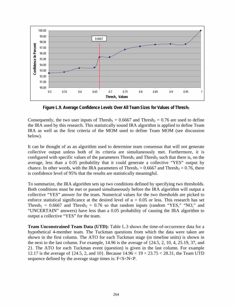
264

90.00

91.00

92.00

93.00

94.00

95.00

96.00

97.00

98.00

99.00

100.00

0.5 0.55 0.6 0.65 0.7 0.75 0.8 0.85 0.9 0.95 1Thresh1 Values

Conf

iden

ce In

Per

cent

0.6667

Figure L.9. Average Confidence Levels Over All Team Sizes for Values of Thresh1

Consequently, the two user inputs of Thresh1 = 0.6667 and Thresh2 = 0.76 are used to define the IRA used by this research. This statistically sound IRA algorithm is applied to define Team IRA as well as the first criteria of the MOM used to define Team MOM (see discussion below). It can be thought of as an algorithm used to determine team consensus that will not generate collective output unless both of its criteria are simultaneously met. Furthermore, it is configured with specific values of the parameters Thresh1 and Thresh2 such that there is, on the average, less than a 0.05 probability that it could generate a collective “YES” output by chance. In other words, with the IRA parameters of Thresh1 = 0.6667 and Thresh2 = 0.76, there is confidence level of 95% that the results are statistically meaningful. To summarize, the IRA algorithm sets up two conditions defined by specifying two thresholds. Both conditions must be met or passed simultaneously before the IRA algorithm will output a collective “YES” answer for the team. Numerical values for the two thresholds are picked to enforce statistical significance at the desired level of α = 0.05 or less. This research has set Thresh1 = 0.6667 and Thresh2 = 0.76 so that random inputs (random “YES,” “NO,” and “UNCERTAIN” answers) have less than a 0.05 probability of causing the IRA algorithm to output a collective “YES” for the team. Team Unconstrained Team Data (UTD): Table L.3 shows the time-of-occurrence data for a hypothetical 4-member team. The Tuckman questions from which the data were taken are shown in the first column. The ATO for each Tuckman stage (in timeline units) is shown in the next to the last column. For example, 14.96 is the average of {24.5, 2, 10, 4, 25.19, 37, and 2}. The ATO for each Tuckman event (question) is given in the last column. For example 12.17 is the average of {24.5, 2, and 10}. Because 14.96 < 19 < 23.75 < 28.31, the Team UTD sequence defined by the average stage times is: F<S<N<P.

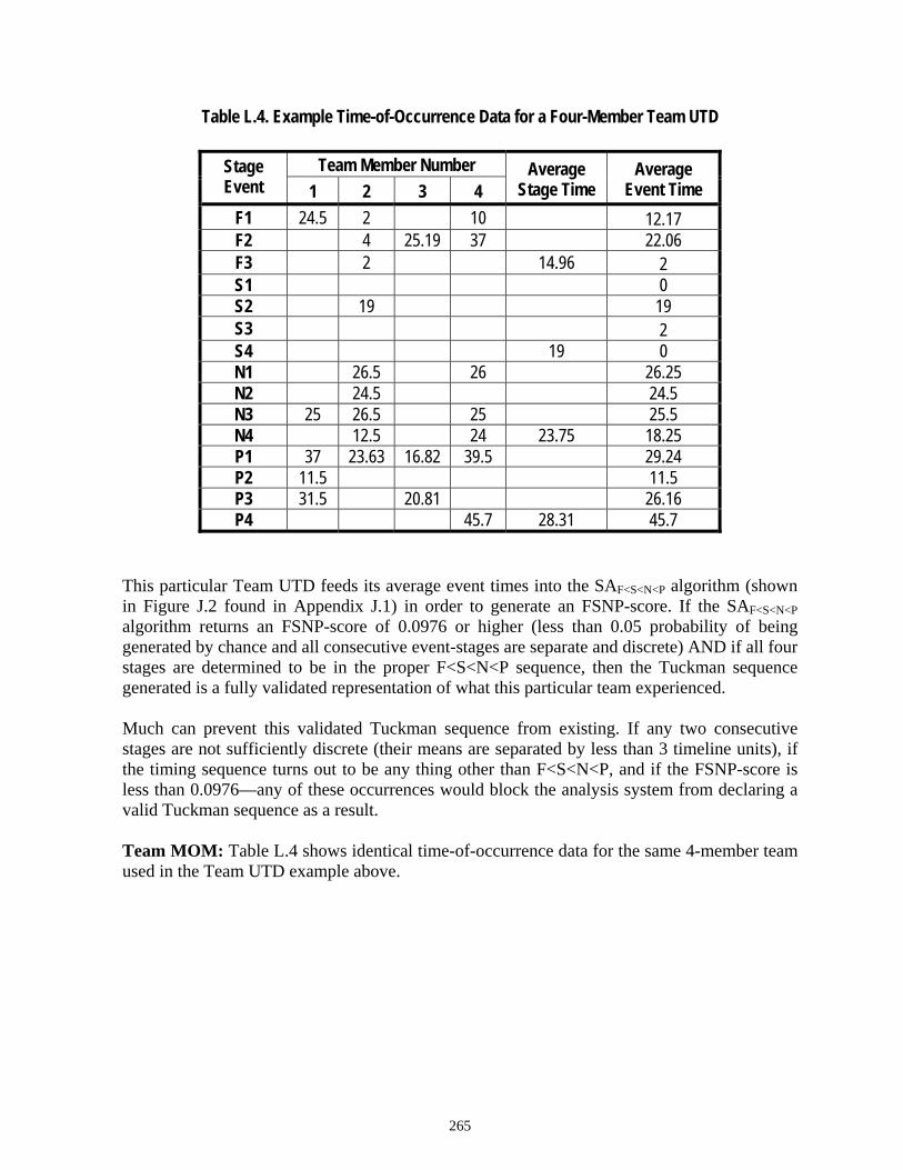
265

Table L.4. Example Time-of-Occurrence Data for a Four-Member Team UTD

This particular Team UTD feeds its average event times into the SAF<S<N<P algorithm (shown in Figure J.2 found in Appendix J.1) in order to generate an FSNP-score. If the SAF<S<N<P algorithm returns an FSNP-score of 0.0976 or higher (less than 0.05 probability of being generated by chance and all consecutive event-stages are separate and discrete) AND if all four stages are determined to be in the proper F<S<N<P sequence, then the Tuckman sequence generated is a fully validated representation of what this particular team experienced. Much can prevent this validated Tuckman sequence from existing. If any two consecutive stages are not sufficiently discrete (their means are separated by less than 3 timeline units), if the timing sequence turns out to be any thing other than F<S<N<P, and if the FSNP-score is less than 0.0976—any of these occurrences would block the analysis system from declaring a valid Tuckman sequence as a result. Team MOM: Table L.4 shows identical time-of-occurrence data for the same 4-member team used in the Team UTD example above.

Team Member Number Stage Event 1 2 3 4

Average Stage Time

Average Event Time

F1 24.5 2 10 12.17 F2 4 25.19 37 22.06 F3 2 14.96 2 S1 0 S2 19 19 S3 2 S4 19 0 N1 26.5 26 26.25 N2 24.5 24.5 N3 25 26.5 25 25.5 N4 12.5 24 23.75 18.25 P1 37 23.63 16.82 39.5 29.24 P2 11.5 11.5 P3 31.5 20.81 26.16 P4 45.7 28.31 45.7

266

Table L.5. Example Time-of-Occurrence Data for a Four-Member Team MOM

As before, the Tuckman questions from which the data were taken are shown in the first column. The ATO for each Tuckman stage and the average event time (in timeline units) are shown in the last two columns. The column labeled “MOM factor” shows the results of the MOM calculation that are independently applied to each stage. Because the MOM factor for Storming is zero, the average stage time for Storming is set to zero and all of the event times for Storming are set to zero. Because the MOM factors for Forming, Norming, and Performing are all ones, the average stage times and all of the event times for Forming, Norming, and Performing are unchanged from the Team UTD example above. Therefore, while Team UTD saw an F<S<N<P Tuckman sequence, Team MOM saw an F<N<P Tuckman Variant 1 sequence. Why was the MOM factor set to zero for Storming? The MOM algorithm imposes a logical OR condition upon three independent criteria. A passing score of 1 in any of the three criteria produces a MOM factor of 1. A failed score of 0 in all of the three criteria produces a MOM factor of 0. The MOM factor is multiplied times the stage time and the event times. Note that in the example given by Table L.4, only one team member answered “YES” to one of the four Storming questions while all other team members answered “NO” to all the Storming questions (team member two answered “YES” to Storming question two). Thus, there was a total of 1 “YES” answer out of a possible total of 16. In other words, 6.25% of the Storming questions were answered “YES” (Storming was observed), and 93.75% of the Storming questions indicated that Storming behavior was not observed by this team.

Team Member Number Stage Event 1 2 3 4

MOM Factor

Average Stage Time

Average Event Time

F1 24.5 2 10 12.17 F2 4 25.19 37 22.06 F3 2 1 14.96 2 S1 0 S2 19 0 S3 0 S4 0 0 0 N1 26.5 26 26.25 N2 24.5 24.5 N3 25 26.5 25 25.5 N4 12.5 24 1 23.75 18.25 P1 37 23.63 16.82 39.5 29.24 P2 11.5 11.5 P3 31.5 20.81 26.16 P4 45.7 1 28.31 45.7

267

The following paragraphs assess an analysis of the MOM factor calculation used in the example provided by Table L.4. Remember, if any of the three criteria is equal to 1, then the MOM factor = 1, and if all three criteria independently equate to zero, the MOM factor = 0. Criteria 1: Criteria 1 applies the same IRA algorithm (with the same input constants of Thresh1 = 0.6667 and Thresh2 = 0.76) that is used to define team IRA (see previous section of this sub-appendix). The IRA determines which, if any, of the 15 Tuckman events described by the 15 Tuckman questions were observed by enough team members to pass both thresholds to earn a collective “YES” from the IRA algorithm. If any stage has at least one of its questions pass the IRA test, then MOM Criteria 1 criterion is given a 1 (pass) for that stage. Consequently, if any one Tuckman event (question) relative to a given stage is observed by enough team members to produce a collective “YES” from the IRA algorithm, then that stage passes the MOM Criteria 1 criteria even if no other questions from that stage were observed. In other words, Criteria 1 supports the existence of a collective stage experience within a team if there is strong agreement (passes IRA test) that a given stage-related event (question) was clearly observed. Using the Storming stage as an example: Thresh1 asks if at least 66.67% of the team had answered “YES” to any Storming question, and Thresh2 asks if the average yes/no/uncertain score produced by averaging the team’s answers for each Storming question (“YES” = 1, “UNCERTAIN” = 2, “NO” = 3) was at least 76% of the way from “NO” toward “YES”; that is, was their average “yes/no/uncertain score” ≤ 1.48 for any question. These threshold values guarantee, with a 95% level of confidence, that random input could not produce a “YES” answer. When the Storming input data implied by Table L.4 (1 “YES” answer and 3 “NO” or “UNCERTAIN” answers for the second Storming question; and 0 “YES” and 4 “NO” or “UNCERTAIN” answers for the rest of the Storming questions) were input into the IRA algorithm, the Storming stage received a MOM factor of zero (all four Storming questions failed to meet both threshold criteria). Because a collective “YES” answer could not be given to any Storming question (Storming input data for a given question must successfully pass both thresholds), MOM Criteria 1 failed and is given a 0 value to numerically express that failure (see Table L.5). [Note: At least one Storming question would have had to produce double ones (a one for passing each of the Thresh1 and Thresh2 criteria) for the Storming stage to pass the MOM Criteria 1 IRA tests. If MOM Criteria 1 had passed its IRA test for the Storming stage, the Storming stage would be given a MOM Criteria 1 factor value of 1 to numerically express its success. That did not happen for Storming in the Table L.4 example (Storming received a MOM Criteria 1 factor of zero), but it did happen for the other three stages.] Criteria 2: In order to pass Criteria 2, the ratio (R) of actual “YES” answers to potential “YES” answers must be ≥ Ratio Threshold1 = RT1 = 0.333 and at the same time the Kappa score (κ) for the stage must be greater than Kappa Threshold1 = κT1 = 0.1225. (There is about a 0.05 probability of achieving a Kappa score of 0.1225 with random answers (see Figure N.2).) Criteria 2 supports the existence of a collective stage experience within a team if a sizeable minority (R ≥ RT1) of team members agrees very strongly (κ > κT1) that a given stage was observed. Appendix N, Figure N.2, provides the Kappa probability distribution.

268

Criteria 3: Criteria 3 is similar to Criteria 2. In order to pass Criteria 3, the Ratio (R) of actual “YES” answers to potential “YES” answers must be ≥ than RT2 = 0.499 and at the same time the Kappa score (κ) for the stage must be greater than Kappa Threshold2 = κT2 = 0.05 (there is about a 36% chance of achieving a Kappa score of 0.05 with random answers, or equivalently there is a 63.8% confidence that a Kappa score of 0.05 was not produced by random answers. Criteria 3 supports the existence of a collective stage experience within a team if a majority (R ≥ RT2) of team members agree to some notable extent (κ > κT2) that a given stage was observed. (See Figure N.2).

Table L.6. Evaluating the MOM Algorithm for Storming

Why the MOM Factor was set to zero for Storming. Table L.5 shows that since all three Storming measure of merit criteria failed the MOM test, the MOM factor for Storming is zero—indicating that giving the Storming stage an average score of 19 (stating that the collective time-of-occurrence value that best represented the entire team’s Storming experience was 19—as was done for Team UTD), has no merit because it misrepresents this particular team’s experience. This methodology takes the position that Team UTD’s collective team Storming score of 19 creates the misleading impression within the analysis that this team experienced Storming at 19 timeline units, when in fact the team members almost unanimously deny that any notable Storming ever took place within the team. Within the MOM methodology, the “NO” answers are allowed to carry at least some weight as to the collective team’s experience. That one “YES” vote means a “YES” for the entire team while only completely unanimous “NO” votes mean a no for the entire team introduces an unreasonable weighting system that gives meaning and significance only to the “YES” answer. The MOM methodology supports the fact that “NO” answers carry at least some significance in calculating an accurate collective team experience. Though there are relatively few occurrences of Storming, they are scattered widely throughout the data; therefore, misleading results like these occur often enough to skew the overall results. The three-criteria MOM algorithm was also applied to the Forming, Norming, and Performing stages of the example and produced a value of 1 for each of these stages. Because 14.96 < 23.57 < 28.31, the Team MOM sequence defined by the average stage times is: F<N<P. This particular Team MOM feeds its average event times into the SAF<N<P algorithm (shown in Figure J.8 found in Appendix J.2) in order to generate an FNP-score. If the SAF<N<P algorithm returns an FNP-score of 4.134 or higher (less than 0.05 probability of being generated by chance and all consecutive event-stages are separate and discrete) AND if

Storming Stage Criteria 1 (IRA) Criteria 2 Criteria 3

Parameter Thresh1 Thresh2 RT1 κT 1 RT2 κT 2

Value .66667 .76 .333 .1225 .499 .05

MOM Factor

Result Failed (0) Failed (0) Failed (0) 0

269

all three stages are determined to be in the proper F<N<P sequence, then the Tuckman Variant 1 sequence generated is a fully validated representation of what this particular team experienced. Much can prevent this validated FNP sequence from existing. If any two consecutive stages are not sufficiently discrete, if the timing sequence turns out to be any thing other than F<N<P, and if the FNP-score is less than 4.134—any of these occurrences would block the analysis system from declaring a valid FNP sequence as a result. To optimize the search for teams following the FNP sequence model, all data were simultaneously run with all Storming values set to zero. Likewise, to optimize the search for teams following the F<N/P sequence model, all of the data with all Storming values set to zero and with all Norming and Performing values grouped together as one N/P stage were analyzed.

270

271

APPENDIX M

DATA QUALITY

272

273

Low quality data are always an important issue. They tend to skew results as well as generate noise or dispersion within the data set. For example, a team member who is trying to minimize the effort and time required to fill out the questionnaire without seeming to be uncooperative may always check box one of the timeline for every randomly selected “YES” answer (see quality filter 3 below). In less than a minute they are done with the questionnaire and are able to take a break or do something else that is more important to them personally. A returned questionnaire, such as this one, or one that contains many procedural errors (a “YES” answer with no timeline data) does not reflect due diligence on the part of the team member submitting it and thus is likely to introduce errors into the collective team result that incorporates this low quality data. Any data that are not input with careful consideration for accuracy become noise in the database. Noise in the database at best obscures honest results and at worst produces misleading results. The first step after data collection is to eliminate as much of the noise (erroneous and misleading data) as possible without modifying the signal (questionnaires reflecting due diligence on the part of the submitter) in any way. It is usually impossible to isolate and then eliminate 100% of the noise. Attempting to do so will toss out too much signal along with the noise, consequently denigrating or modifying the signal in the process. The processes used in this research to reduce the noise in the collected data are carefully designed and tested (by manual inspection) to eliminate only the most obvious and egregious noise sources. Calculating the results with and without the data quality filters turned on clearly demonstrates that the removal of noise significantly reduces data dispersion by 10 to 25% (as measured by the standard deviation of time-of-occurrence data and timeline stage separation data, and by changes in the Kappa statistic’s measurement of agreement) and clearly contributes to the quality and clarity of the final results. Four types of automated data quality filters were defined (see Figure M.1). Each filter was carefully designed to eliminate a particular type of “noise” from the collected data. About 18% of the original data collected were discarded because of their low quality. The four quality filters functionally operate in series and, thus, together constitute one overall filter that only passes or outputs data that simultaneously meet the criteria (expressed as threshold requirements) of all four.

Figure M.1. Four Independent Quality Filters in Series

Quality Filter 4

Quality Filter 3

Quality Filter 2

Quality Filter 1

Input All Data

Output to Research Data Base

Reject Poor Quality Data

Reject Poor Quality Data

Reject Poor Quality Data

Reject Poor Quality Data

274

Quality Filter 1—Errors: The first type of poor quality input was produced by team members not taking the time and due diligence to answer the questionnaire properly. Such input data were full of errors. There were three types of “fatal” errors: 1) A “YES” answer was given, but no time-of-occurrence data were indicated on the timeline, 2) A “NO” answer was given; however, time-of-occurrence data were indicated on the timeline. 3) Questions were skipped altogether with no answer and no timeline data.

Filter 1 Thresholds: If more than 20% of the 15 Tuckman questions had such fatal errors (Tuckman Error Threshold (TET) = 3), the data were eliminated from consideration. If more than 20% of the total 31 questions represented fatal errors (Total Error Threshold (ToET) = 6.2), the data were eliminated from consideration.

Quality Filter 2—Non-cooperation Strategy 1: The second type of poor quality input was produced by team members who simply answered “NO” or “UNCERTAIN” to almost all of the questions thereby avoiding having to generate the more difficult and time consuming time-of-occurrence data. With all or almost all “NO” or “UNCERTAIN” answers given, the questionnaire produces little or no useful time-of-occurrence data—no sequences of Tuckman stages are defined—there is simply nothing to analyze. It is assumed that most team members falling into this category simply wanted to “get through” the questionnaire as quickly (and with as little effort) as possible. It is possible (although highly unlikely) that a few team members may have been genuinely unable to relate the questions asked to their teaming experience. That this behavior is highly unlikely is based on the exceptionally high Kappa scores, which indicate that the vast majority of team members not only understood the questions clearly, but also understood how their team’s behavior related to the questions. Perhaps a very, very few exceptionally unaware individuals had their questionnaires unfairly rejected, but in the end it makes little difference—there is little that can be done with a questionnaire that produces no useful data.

Filter 2 Threshold: If more than 80% of the total 31 questions were answered with a “NO” or “UNCERTAIN” (N + U = 24.8), the data were eliminated from consideration.

Quality Filter 3—Non-cooperation Strategy 2: The third type of poor quality input was produced by team members who generated the same timeline data for all or almost all of the questions thereby creating little or no useful timeline data for this research. (All stages had the same time-of-occurrence; therefore, no sequence of stages could be defined.) It would appear that most individuals generating entirely redundant time-of-occurrence data simply wanted to “get through” the questionnaire as quickly (and with as little effort) as possible.

275

For example, such individuals may have checked timeline box 1 for every “YES” answer indicating that all four of the Tuckman stages happened immediately, all at once, and never happened again. In this case, it is reasonable to assume that the “YES” answers were most likely chosen at random. Also, at the opposite end of the scale, there were a few who could not differentiate the stages and felt that every stage happened all the time. These individuals checked all 50 timeline boxes for every “YES” answer. Eventually, that would grow tiresome and they would check just box 1 and box 50. It is possible (although highly unlikely) that a few team members may have been genuinely unable to relate the questions asked to their teaming experience. That this behavior is highly unlikely is based on the exceptionally high Kappa scores, which indicate that the vast majority of team members not only understood the questions clearly, but also understood how their team’s behavior related to the questions. Perhaps a very, very few exceptionally unaware individuals had their questionnaires unfairly rejected, but in the end it makes little difference—there is little you can do with a questionnaire that produces no useful data. It should be noted that many of the filled out questionnaires rejected by quality filter 3 were also rejected by quality filters 1 and 2.

Filter 3 Threshold. If the team member did not differentiate at least three of the four Tuckman stages, their data were eliminated from consideration. In other words, their timeline data were required to generate at least a three-stage sequence [Cooperation and Awareness Threshold (CAT) = 3]. An analysis of all (unfiltered) input data indicates that generating at least a three-stage sequence is nearly unavoidable for any team member using due diligence in filling out the questionnaire. To produce a three-stage sequence, an individual must relate at least 1 of the 15 questions related to three of the four Tuckman stages and give those different times-of-occurrence. Ninety-eight percent of all questionnaires that were properly filled out (passed the error criteria of filter 1 and filter 2 defined above) accomplished this and produced a three-stage sequence—it was only the individuals who generated an identical average time-of-occurrence for all (or almost all) Tuckman events that were eliminated from the database because of highly suspicious repetition. Individuals who were dropped due to this quality criterion were manually checked. Almost all were found to be clear and obvious cases of non-cooperation or “gaming” the questionnaire—very few produced data that were difficult to interpret as gaming.

Quality Filter 4: A fourth type of quality check was applied to the teams as a whole instead of to the input data. If, after the three sets of quality checks described above were applied and all individual team members producing poor quality data had been dropped from the database, at least 50% of the original team members (not just those who submitted a questionnaire) were not still present in the research database, the team was disqualified and dropped from consideration. This filter ensures that a team cannot be represented by a minority of its members.

276

Filter 4 Threshold. Set a Minimum Team size (MT). In other words if more than 50% (MT = 50%) of the original team members either did not submit a questionnaire or produced unacceptable quality data, the team was disqualified and eliminated from consideration as a valid team.

When designing data quality filters, it is important not to introduce any biases or systematic errors into the data through the selective elimination of certain types of data. Human errors and inconsistencies are eliminated by employing algorithms. Systematic errors are eliminated by keeping the filters simple and straightforward, eliminating data only for the most obvious and blatant of problems, never filtering on a parameter that directly impacts the results, and by performing many manual checks to make sure the filters are doing only what they were designed to do.

277

Respondent Databases Three databases were assembled to support this research project:

● Database 1: The master set, which contains every questionnaire submitted by team members.

● Database 2: A subset of the master set that contains only those questionnaires that meet

all individual data quality standards (have successfully passed through data quality filters 1, 2, and 3).

● Database 3: A subset of database 2 that is limited to individuals who are part of a valid

team. A team is valid if all of its current members come from database 2 and if it contains responses from at least 50% of its original members (i.e., total number of team members, whether they responded to the questionnaire or not). Equivalently, every team in database 3 has successfully passed through data quality filter 4. Furthermore, its members have all individually passed through data quality filters 1, 2, and 3.

Analysis of individual data was performed within database 2. Analysis of team data was performed within database 3. Because this research is about observing and evaluating the dynamics of teams, database 3 is referred to as the research database—the database from which the results and conclusions of this research are drawn. The relationships among the three databases are explained below. The questionnaire response rate is calculated by dividing the number of people who submitted questionnaires by the number of people who were part of the teaming activity investigation (those who were asked to fill out a questionnaire). The questionnaire response rate is 89.82%. The respondent quality rate is the percentage of all individuals who submitted questionnaires that successfully passed through data quality filters 1, 2, and 3 to make it into database 2. The respondent quality rate is 81.67%. In other words, 18.33% of the questionnaires submitted were found to be of poor enough quality that they had to be eliminated from consideration.

● Database 1 contains 1,974 original team members who were grouped into 368 teams. Of these 1,974 individuals, 1,773 (89.82%) returned questionnaires.

● Database 2 contains 1,448 individuals who are grouped into 368 teams.

● Database 3 contains 1,367 individuals who are grouped into 321 valid teams.

In going from Database 1 to Database 2: Five hundred twenty-six (26.65%) of the original team members were not included in database 2. Of these, 325 (16.46% of the original team members) did not fill out questionnaires while 201 (10.18% of the original team members) produced questionnaires of unacceptable quality.

278

However, the 526 dropped team members were scattered more or less evenly across all the teams. In going from Database 2 to Database 3: Eighty-one (5.59%) of the individuals and 47 (3.25%) of the teams were dropped. A team was dropped from inclusion in database 3 if the number (of a given teams’ members) responding with acceptable quality questionnaires was less than half of the original team members. In other words, after subtracting those who did not return a questionnaire and those who returned an unacceptable questionnaire, one still needed to have half or more of the original team members representing the team before that team was allowed to participate in this research. In going from Database 1 to Database 3: Six hundred and seven (30.75%) of the original team members were not included in database 3, and 47 (12.77%) of the 368 teams were dropped from final consideration. The high response rate of 89.82% was due to group members being asked to fill out their questionnaires immediately after completing their team project. Team members are in a situation where being seen as a non-contributor may have a moderate to serious negative impact. However, since the questionnaire was submitted anonymously, those who wished to avoid the effort of participating simply “gamed” the process rather than appear non-cooperative. That only 12.77% of the teams were dropped due to a combination of non-responsiveness and poor quality demonstrates a high level of diligence and overall good attitude shown by the DAU students toward the extra time and effort (about 20 minutes to fill out the questionnaire) this research required. Data Quality vs. Team Performance Quality. Each team was required to produce a set of products relevant to each course and specific to the teaming exercise performed. The quality of the processes used and the products produced by each team were critiqued by course instructors and then graded (below average, average, and above average) by the lead instructor. An interesting observation is that a team being dropped from the database because of poor response and/or poor quality responses is not an indicator of below average performance as is shown by Table M.1. This table addresses the question: Of the teams that were dropped from consideration, how many were rated above average, average, or below average by their instructors? In the research population (database 3), 45% produced above average products during their team activity, 47% produced average products, and 8% produced below average products. In Table M.1, the data indicate that 45% of the dropouts produced above average products, 53% of the dropouts produced average products, and only 2% of the dropouts produced below average products. It appears that average performers were a little more likely to be tossed out of the database than above average performers, but that below average performers were much less likely to be

279

bounced out due to poor participation and poor quality data than teams who produced average or above average products. Perhaps the below average performers were simply less experienced personnel (i.e., less competent) and thus trying harder to make up for that deficiency. Consequently, their difficulty in producing good products was not reflective of a lack of due diligence (careless approach or a poor attitude), which is more likely to lead to a team being dropped.

Table M.1. Instructor Evaluation of Dropped Teams’ Products

Above Average Average Below Average Number 21 25 1 Percent 45% 53% 2%

280

281

APPENDIX N

ABILITY OF DATA COLLECTION METHODOLOGY

TO SUPPORT RESEARCH GOALS

(LIMITATIONS OF THE METHODOLOGY)

282

283

A. Measurement Accuracy Whenever questionnaires are employed to collect data, one must address the issues of data quality and the ability of the data to support the stated research goals (determining if Defense Acquisition University (DAU) teams follow Tuckman’s sequential stages model) in a statistically rigorous manner. All team members may not approach the questionnaire with the same degree of exactitude and due diligence. While some may make unintentional errors, a few may very quickly fill out the questionnaire without even reading the questions in order to appear to be cooperating and participating while minimizing the time and effort required. Lack of due diligence, whether intentional or not intentional, produces “noise” in the data. When using questionnaires to collect data, one expects some variance in the responses given by individual team members. Asking team members to specify the time-of-occurrence of each Tuckman stage at the end of the teaming experience, requires significant skill in clearly identifying specific team behaviors and accurately remembering when they occurred. Variations of attention, perception, interpretation, language use, and understanding among team members also produce “noise” in the data. Relative to both sources of noise (in order to validate the chosen data collection methodology), it must be mathematically demonstrated that the variations among questionnaire responses (to the same questions) among the members of a single team, are small enough to support rigorous unambiguous research results and conclusions. The extent to which the methodology, data collection instrument, and analysis are capable of accurately detecting and measuring the existence of Tuckman sequences within the DAU data must be determined. Limitations inherent within the data collection and analysis process must be discovered, measured, and clearly stated. To that end, two separate assessments were performed to answer the following questions:

1. Are the team members aware of the Tuckman stages that they are experiencing within their teams; do they agree on the interpretation of that experience; and are they able to accurately relate that experience to the individual questions within the questionnaire instrument? Kappa analysis will be employed to make this determination.

2. Are the team members able to specify the time-of-occurrence of the Tuckman stages

accurately enough to clearly define a sequence of observed events? An analysis of the variance of the timing data generated by team members for each stage within each team, and the variance of each team’s collective timing data will be employed to make this determination. B. Kappa Analysis A Kappa Analysis was performed to determine the extent to which the two following conditions were met:

1. The team members understood what the Miller (1997) Group Process Questionnaire (GPQ) questions are asking, or said another way, whether or not the team members interpret the questions the same way (agreement).

284

2. The team members (who are not experts in group dynamics) were able to clearly assess

the dynamics of their team experience and successfully associate that experience with the GPQ questions. The Kappa statistic measures the consistency and agreement between a group of κ independent raters evaluating N questions, which each have m possible answers (such as “YES, NO, or UNCERTAIN”). A lack of knowledge and understanding among the team members would, most reasonably, be expected to create vagueness, uncertainty, and non-uniformity (disagreement) among the answers produced by a given team. The assumption is that team members would not show strong agreement in their answers to the questionnaire if they could not clearly understand the questions or if they were unable to clearly relate the questions to the behavior they witnessed in their team experience. A lack of uniformity in the team’s answers would be directly related to the amount of randomness within the data. Exceptionally strong team agreement, on the other hand, would indicate that the interface between actual team behavior and the questionnaire instrument was more or less universally clear and well understood. Only if all the team members observe and interpret the same behaviors in the same way will they be likely to strongly agree on how the questions should be answered. Because of the simplicity and straightforwardness of the required observations and because of the proven validation of the GPQ instrument (Miller 1997), a false positive is extremely unlikely, i.e., that most team members would consistently and uniformly make the same erroneous observations about what their team experienced in the same way at the same time. The Kappa statistic (Cohen 1960) was applied to the DAU data by independently assessing each of the Tuckman stages and all the stages combined for each team. To determine the significance of a Kappa score, the random Kappa distribution shown in Figure N.1 was created by creating 117,200 five-person teams. Each of the 5 team members randomly chose “YES,” “NO,” or “UNCERTAIN” answers. The Kappa value assessing agreement for each team was calculated. The resultant 117,200 Kappa scores were sorted into bins to produce the random Kappa distribution.

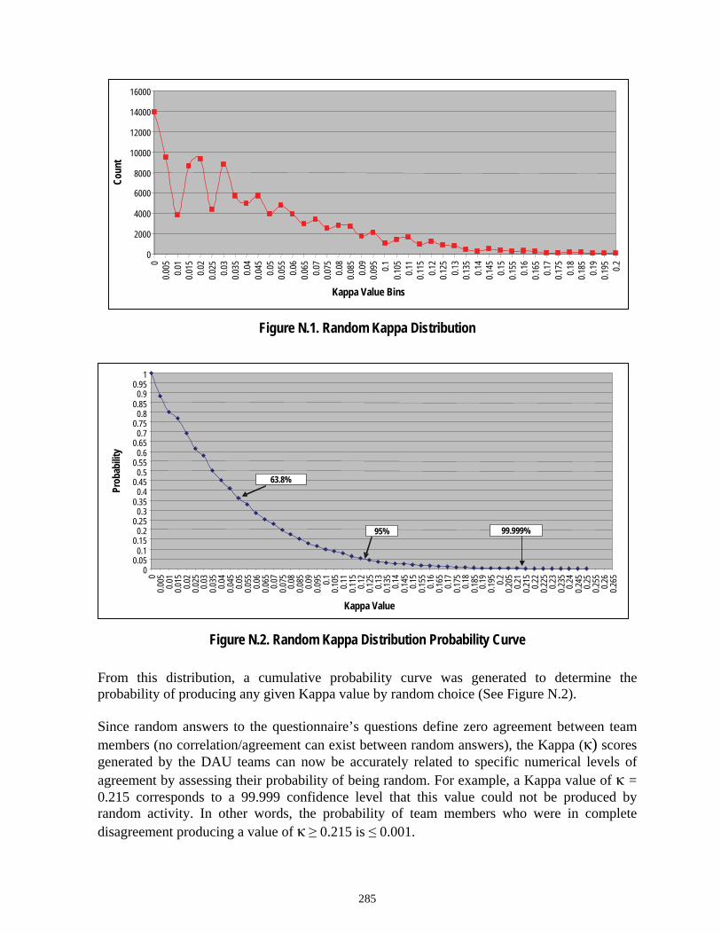
285

0

2000

4000

6000

8000

10000

12000

14000

16000

00.0

05 0.01

0.015 0.0

20.0

25 0.03

0.035 0.0

40.0

45 0.05

0.055 0.0

60.0

65 0.07

0.075 0.0

80.0

85 0.09

0.095 0.1

0.105 0.1

10.1

15 0.12

0.125 0.1

30.1

35 0.14

0.145 0.1

50.1

55 0.16

0.165 0.1

70.1

75 0.18

0.185 0.1

90.1

95 0.2

Kappa Value Bins

Coun

t

Figure N.1. Random Kappa Distribution

00.05

0.10.15

0.20.25

0.30.35

0.40.45

0.50.55

0.60.65

0.70.75

0.80.85

0.90.95

1

00.0

050.0

10.0

150.0

20.0

250.0

30.0

350.0

40.0

450.0

50.0

550.0

60.0

65 0.07

0.075

0.08

0.085

0.09

0.095 0.1

0.105

0.11

0.115

0.12

0.125

0.13

0.135 0.1

40.1

45 0.15

0.155 0.1

60.1

65 0.17

0.175 0.1

80.1

850.1

90.1

95 0.20.2

050.2

10.2

150.2

20.2

250.2

30.2

350.2

40.2

45 0.25

0.255

0.26

0.265

Kappa Value

Prob

abilit

y

63.8%

95% 99.999%

Figure N.2. Random Kappa Distribution Probability Curve

From this distribution, a cumulative probability curve was generated to determine the probability of producing any given Kappa value by random choice (See Figure N.2). Since random answers to the questionnaire’s questions define zero agreement between team members (no correlation/agreement can exist between random answers), the Kappa (κ) scores generated by the DAU teams can now be accurately related to specific numerical levels of agreement by assessing their probability of being random. For example, a Kappa value of κ = 0.215 corresponds to a 99.999 confidence level that this value could not be produced by random activity. In other words, the probability of team members who were in complete disagreement producing a value of κ ≥ 0.215 is ≤ 0.001.

286

The average random value of Kappa = 0.044; it has a 0.425 probability of being random or a 0.57% confidence level of not being random. [Because Kappa is not a linear function, its average random value does not have to have a probability of 0.5.] A Kappa value of κ = 0.05 is slightly larger (less likely to be random) than the average random value of Kappa (0.044) and has a 0.36 probability of being random (a 64% confidence of not being random)—a good value to specify when minimal agreement that is still above random noise is required. The results of the Kappa assessment of the DAU teams are clearly seen in Figure N.3. All the Kappa scores over all DAU teams for each stage separately and for all stages collectively were averaged.

0

0.1

0.2

0.3

0.4

0.5

0.6

0.7

Forming Storming Norming Performing All Stages

Team

Kap

pa V

alue

DAU Teams Random

99.999%

95.0%57.5%

Figure N.3. Kappa Statistic Measure of Agreement

The collected data produced average Kappa scores between 0.47 and 0.64 for all stages (indicating extremely strong agreement of >> 99.999%). It is clear that the team members understood what they were experiencing within their teams, that they agreed on the interpretation of that experience, and that they had no trouble relating that experience to the individual questions within the GPQ instrument. C. Variance within the Time-of-Occurrence Measurements for Each Stage

1. Defining Valid Tuckman Sequences

The Tuckman model requires that four functionally distinct and clearly visible stages occur sequentially in time such that F<S<N<P (where the letters F, S, N, P represent the time-of-occurrence of the Forming, Storming, Norming, and Performing stages). From this definition, given by Tuckman in 1965, two criteria for a valid Tuckman sequence can be derived.

a) The four stages must occur in the proper sequence.

287

b) The stages must be discrete (functionally distinct and clearly differentiable in time). Without the second requirement, unique temporal stages cannot be measured and thus cannot be defined to exist from a scientifically rigorous viewpoint.

Each of the 15 GPQ Tuckman questions describes an event that is related to one of the four Tuckman stages. The reliability tested and validated GPQ ensures that each event-stage whose time-of-occurrence is being measured represents its proper stage behavior (F, S, N, or P). Likewise, satisfying the requirement that the event-stages of a validated Tuckman sequence must occur in the proper sequence is a matter of simply comparing the magnitude of the times-of-occurrence for each event-stage and validating only those that occur in the right order (F<S<N<P) as Tuckman sequences. However, that leaves one condition for a valid Tuckman sequence still unspecified. How will one determine if the stages are clearly defined in time, i.e., if they are discrete stages? The data collected by the GPQ must be able to “adequately” measure whether or not consecutive stages can be clearly resolved into distinctively separate stages capable of defining a meaningful sequence. One must precisely define the conditions that determine when two broadly overlapping stages can be said to be separated in time such that they form two distinct and separate stages to some specified level of statistical confidence. Certainly, any test for reasonableness would fail to be met if one imagines a real-world team experiencing consecutive Tuckman stages that were separated by only a small fraction of a second—especially when one considers the rational requirements for an “interactive team experience” to have taken place during that fraction of a second, and the natural error, uncertainty, and variance within the measured time-of-occurrence data. Obviously, one stage having an average time-of-occurrence that is 0.01 timeline units greater than the previous stage can not credibly define (or resolve in time) a real sequence of discrete stages within a team’s experience—and most certainly not if that time-of-occurrence data were measured by the Miller GPQ. Specifically, when applying the GPQ after the task is completed, there is too much uncertainty or randomness in the measured (recorded) time-of-occurrence data to define sequences based upon a single timeline unit, much less fractions of a timeline unit. Undoubtedly, some minimum stage separation is required to define a “valid” sequence of Tuckman stages. In order to develop statistically rigorous criteria that determine whether or not any given sequence of Tuckman stages is “adequately” separated in time, one must first understand the sources of error, randomness, and limits of measurement capability that are inherent to one’s measurement methodology. Measurement error, randomness, and the limits of measurement capability together produce what is called “noise” in the measured data, which leads to some level of uncertainty in the research results and places limitations upon the research’s conclusions. Thus an accurate measurement of the noise inherent to the GPQ measurement methodology is not only critical to the definition of what this research can consider a “valid” sequence of stages, but also to a meaningful interpretation of the research’s results and conclusions.

288

2. Sources of error and error assessment methodology. There were three major sources of noise:

a. Operational: Small- to medium-sized teams produce a small number of data points defining each stage. This leads to noisy population means that are not well defined. Small quantities of time-of-occurrence data per stage per team (ni) are an artifact of small team size for all stages and due to the lack of Storming behavior for the Storming stage. Remember, the Storming stage must be found to be discrete in time to a confidence level of 95% relative to Forming and Norming, and the Norming and Performing stages must be successfully separated before a valid Tuckman sequence can be defined. These requirements were made difficult to achieve because: 1) though all the stages had small values of ni, there was an average of only 2 data points (n2 = 2) in the Storming stage making the Storming mean particularly imprecise and noisy; 2) the average Norming and Performing means were separated by only 2.37 timeline units; and 3) the Storming and Performing stages were likely to be grouped together into one stage since the means of their time-of-occurrence data (for teams) were separated by less than 0.7 timeline units. The Storming and Norming stages were also likely to be grouped together into a single population (given the particularly noisy Storming time-of-occurrence data) since the means of their time-of-occurrence data (for teams) were only separated by 1.72 timeline units. To untangle these difficulties, one would like to have low noise data producing sharp accurate means.

b. Data collection: There were several noise sources in the time-of-occurrence data that

were inherent to the methodology used to collect the data (Miller GPQ implementation—see Chapter IV and Appendix Q for a full discussion of the data collection methodology). These are: 1) having team members fill out the questionnaire after their teaming activity was completed instead of immediately after the event was observed; 2) using a 50-unit timeline instead of natural real-time; 3) having only 15 Tuckman-related questions out of 31 questions total; and 4) the fact that it is often difficult, even for highly trained experts, to accurately specify the time-of-occurrence of a Tuckman stage because the initiation (in time) of a Tuckman stage is often a subtle event without clear or reliable markers and is therefore dependent upon a highly subjective assessment. All four error sources produced largely random errors that contributed to the level of noise in the data.

c. Analysis: Some analysis methodologies reduce the levels of noise while others

increase noise levels. Measuring time-of-occurrence by picking the first time-of-occurrence is the most noise prone methodology. Using the median to combine multiple times-of-occurrence marked on a timeline is the second noisiest methodology. Averaging time-of-occurrence data is the least noisy analysis methodology. More details are provided in Appendix L.

Consequently, considerable variance in the time-of-occurrence data for both teams and individuals was expected. A mathematical process, similar to the Kappa analysis described earlier in this chapter, was used to assess how much noise, randomness, or lack of coherent content was contained within the DAU data. The general process works like this: The results generated by each independent

289

measurement and analysis process implemented within the DAU dataset was compared to the results generated by a similar process applied to a reference dataset composed entirely of random numbers. The results generated by the reference dataset were repeated a large number of times (e.g., 150,000) using a different set of random numbers each time. The 150,000 random results were then sorted into bins thus forming a distribution of random results. This distribution was then numerically integrated to produce a cumulative probability curve. The probability curve enables a numerically expressed statistical comparison between results produced by the DAU dataset (which contains information and noise) relative to the reference dataset (which contains only noise). In other words, the application of this mathematical process enables the determination that results based upon the DAU data are, to a certain level of statistical confidence, not random (not derivable from random input). Or equivalently, that the probability of the results being random (that they are based on noise rather than information) is equal to or less than some specific number α. For this research, α was set equal to 0.05. This means that the probability of the research results being derivable from uncorrelated or random data must be ≤ 0.05 or the results are deemed statistically insignificant and tossed out. Equivalently, the confidence that these research results are not derivable from random data must be ≥ 95%. For example, the statistical methodology just described was employed earlier in this appendix to assess the statistical significance of the Kappa calculation. This methodology is used many times within this research to generate a particularly useful distribution and then integrate that distribution to produce cumulative probability curves, which enable accurate assessments of the statistical significance of the measured results.

3. Assessing noise levels within the DAU data. It is assumed that the variance of the measured time-of-occurrence data is a direct measure of the overall noise inherent within the research measurement process. Subsections a), b), and c) below outline three independent approaches to assessing the variance of time-of-occurrence data in order to measure how accurately and consistently DAU team members were able determine the time-of-occurrence of the 15 Tuckman events described by 15 Tuckman questions.

a) The first approach calculates the variation within the timing data generated by each DAU team by computing the variance in the event timing data for each Tuckman stage (see the derivations of equations L2.14 through L2.17 in Appendix L.2). The variances for each stage averaged over all teams (see the derivations of equations L2.18 through L2.21, column A, in Appendix L.2) was then compared to the variance that would be generated if the timing data were random. Thirty thousand 5-person teams (150,000 independent questionnaires) with randomized timing data were used to generate both a reference distribution and a cumulative probability curve that enabled the association of a given value of measured variance with the probability that this value could be produced by random time-of-occurrence data.

(1) Assessing average noise levels within the time-of-occurrence data. First one has to

determine if there is enough real information (signal) within the time-of-occurrence data to

290

support statistically significant conclusions. In an effort to determine the relative amounts of signal to noise within the time-of-occurrence data, 150,000 questionnaires were randomly answered “YES,” “NO,” or “UNCERTAIN.” However, because the intent was to assess the level of noise contained within a team’s time-of-occurrence data, the numbers of random “YES,” “NO,” or “UNCERTAIN” answers were constrained to be in the same ratio to each other as the numbers of “YES,” “NO,” or “UNCERTAIN” answers naturally occurring in the DAU data. Each random “YES” answer to a given question was then provided a random time-of-occurrence for the event specified by the question. The distribution and probability curves are shown in Figures N.4 and Figure N.5 respectively.

050

100150200250300350400450500

0 10 20 30 40 50 60 70 80 90 100

110

120

130

140

150

160

170

180

190

200

210

220

230

240

250

260

270

280

290

300

310

320

330

340

350

360

370

Variance Bins

Num

ber o

f Cou

nts

Figure N.4. Reference Distribution of Average Times-of-Occurrence for Random 5-Person Team

0

0.050.1

0.150.2

0.25

0.30.35

0.40.45

0.5

0 10 20 30 40 50 60 70 80 90 100

110

120

130

140

150

160

170

180

190

200

210

220

230

240

250

260

270

280

290

300

310

320

330

340

350

360

370

Variance Bins

Prob

abilit

y

Figure N.5. Cumulative Probability for Random 5-Person Team For example, the probability of random time-of-occurrence scores producing a variance of ≤ 60 or ≥283 is 0.05 or less. Equivalently, there is a 95% or greater confidence level that a

291

variance generated by random activity will be between 60 and 283. Thus, one can now assess the probability that the measured variance of a team’s time-of-occurrence data represents signal rather than noise (could not be generated by random processes). The results of the variance assessment of the DAU teams’ stage time-of-occurrence data are shown in Figure N.6. Here all the individual DAU teams’ variance scores were averaged for each stage separately and for all stages collectively.

0

20

40

60

80

100

120

140

160

180

200

Forming Storming Norming Performing All Stages

Aver

age V

arian

ce

DAU Teams Random

Figure N.6. Variance of Timing Data Generated within Teams

From Figures N.4, N.5, and N.6, it can be seen that:

● The typical DAU team variance for all stages is about 99.

● DAU Forming variance (89.98) is at the 91% confidence level that such a small variance could not have occurred by chance.

● DAU Storming variance (64.78) is at the 95% confidence level that such a small

variance could not have occurred by chance.

● DAU Norming variance (117.72) is at the 86% confidence level that such a small variance could not have occurred by chance.

● DAU Performing variance (96.29) is at the 90% confidence level that such a small

variance could not have occurred by chance. ● Variance over all stages (99.25) is at the 90% confidence level that such a small

variance could not have occurred by chance.

292

The time-of-occurrence data generated by the typical DAU team has a standard deviation of 9.5 timing units and a probability of 0.1 of being generated randomly. The measured level of variance in the DAU timing data produces an overall 90% confidence that the measured occurrences of discrete Tuckman stages are real (as opposed to random) events. Since the median duration of DAU teams was 4 hours, the GPQ produces a median timeline resolution of 4.8 minutes or a timeline measurement accuracy of ± 2.4 minutes. Thus, a Standard Deviation of 9.5 timing units represents a one sigma measurement accuracy of ± 22.8 minutes of real-time. Thus, on the average, the team members within the 321 qualified teams studied by this research, generally agreed on the time-of-occurrence of any given Tuckman event to within about 23 minutes (less than 10%) of a 240-minute team duration.

(2) Assessing minimum Stage Separation required to ensure discrete stages given that

the average time-of-occurrence data defining a stage have a standard deviation of 9.5 timeline units. To determine how difficult it is to recognize individual distributions when they are located very close to a similar distribution on the same timeline (representing two closely spaced adjacent Tuckman Stages), two normal distributions whose means were separated by various values of Minimum Stage Separation (MSS) were plotted. These four sets of curves (see Figure N.7) provide an assessment of the minimum separation between consecutive stage means required to be able to clearly resolve discrete stages. It would appear from Figure N.7 that consecutive stage means with a standard deviation of σ = 9.5 would need to be separated by two or three timeline units before one could claim that two discrete stages existed within the combined data.

293

Two normalized normal distributions whose means are separated by the constant MSS = 1

00.10.20.30.40.50.60.70.80.9

11.1

0 2 4 6 8 10 12 14 16 18 20 22 24 26 28 30 32 34 36 38 40 42 44 46 48 50Timeline Units

Normal Dist 1 Normal Dist 2

Two normalized normal distributions whose means are separated by the constant MSS = 3

00.10.20.30.40.50.60.70.80.9

11.1

0 2 4 6 8 10 12 14 16 18 20 22 24 26 28 30 32 34 36 38 40 42 44 46 48 50Timeline Units

Normal Dist 1 Normal Dist 2

Two normalized normal distributions whose means are separated by the constant MSS = 5

00.10.20.30.40.50.60.70.80.9

11.1

0 2 4 6 8 10 12 14 16 18 20 22 24 26 28 30 32 34 36 38 40 42 44 46 48 50Timeline Units

Normal Dist 1 Normal Dist 2

Two normalized normal distributions whose means are separated by the constant MSS = 7

00.10.20.30.40.50.60.70.80.9

11.1

0 2 4 6 8 10 12 14 16 18 20 22 24 26 28 30 32 34 36 38 40 42 44 46 48 50Timeline Units

Normal Dist 1 Normal Dist 2

Figure N.7. Four Sets of Normal Distributions with Standard Deviation = 9.5 and with Mean Separations of 1, 3, 5, and 7 Timeline Units

Here normal distributions were used to model the timing data. The actual time-of-occurrence data generated by a 5-person team for a given stage contain no more than 20 time-of-occurrence measurements and often less than 10 (with an overall average of 9.1 data points per stage). Such small quantities of data do not produce enough data to define a distinctive distribution; consequently, each data set produced by a team for each stage is unique in its shape. Because team members independently fill out the GPQ, it is expected that their attempts to specify (by marking a 50-unit timeline at the end of their teaming experience) when a specific event happened would fall randomly about the actual time, thus generating a roughly normal distribution (if there were enough data, i.e., a large enough number of team members to actually define a distribution). Consequently, there is some justification for modeling a stage’s time-of-occurrence data (represented here as a mean associated with a standard deviation) as a normal distribution in order to help determine a reasonable MSS value.

b) Next, the distribution of the standard deviation (of the time-of-occurrence data) generated by each team for each stage will be examined. Developing a cumulative probability for this distribution will enable an assessment of the maximum and minimum standard deviations (of the time-of-occurrence data generated by each team for each stage) that are likely (P ≥ 0.05) to occur in the DAU data.

(1) Assessing the standard deviation of individual team time-of-occurrence data. The

probability of obtaining a certain value of σ for each time-of-occurrence measurement by the Miller GPQ can be determined by sorting the measured values of σ from all teams into time-

1 2 1 2

1 2 1 2

294

of-occurrence bins (see the derivations of the variance equations L2.14 through L2.17 in Appendix L.2. The standard deviation is computed by taking the square root of each of the four variance equations). This result is shown in Figure N.8.

02468

1012141618202224262830

0 5 10 15 20Standard Deviation in Timeline Units

Num

ber o

f Occ

urre

nces

Forming Storming Norming Performing

STDEV (orig data): 3.13 2.31 2.65 2.86Mean (orig data): 8.95 7.71 10.52 9.39Median (orig data): 9.02 7.78 10.58 9.43

Figure N.8. Distribution of the Standard Deviation of Time-of-Occurrence Data by Stage The average over all four stages produces a standard deviation of 9.5 timeline units as mentioned above. The cumulative probability curves derived by integrating over each distribution are shown in Figure N.9. Table N.1 extracts results from the probability curves.

00.05

0.10.15

0.20.25

0.30.35

0.4

0.450.5

0 2 4 6 8 10 12 14 16 18 20Standard Deviation in Timeline Units

Cum

ulat

ive p

roba

bilit

y

Forming Undefined Storming Undefined Norming Undefined Performing Undefined

Figure N.9. Probability of Occurrence within DAU Data of Various Values of Standard Deviation

295

Table N.1. Confidence (1-Probability) that a Team's Time-of-Occurrence Data Defining Each

Tuckman Stage Will Have a Standard Deviation (σ ) between σ Low and σ High

Confidence Forming Storming Norming Performing All Stages 0.5 8.95 7.71 10.52 9.39 9.50

0.75 6.75 ≤ σ ≤ 10.75 5.5 ≤ σ ≤ 8.75 8.3 ≤ σ ≤ 12 7.2 ≤ σ ≤ 11.2 .5 ≤ σ ≤ 12

0.8 6.4 ≤ σ ≤ 11.25 5.25 ≤ σ ≤ 9.75 8 ≤ σ ≤ 12.4 6.5 ≤ σ ≤ 11.75 5.25 ≤ σ ≤ 12.4

0.9 4.75 ≤ σ ≤ 12.75 3.5 ≤ σ ≤ 10.5 7 ≤ σ ≤ 13.6 8 ≤ σ ≤ 12.75 3.5 ≤ σ ≤ 13.6

0.95 3.25 ≤ σ ≤ 14 2.75 ≤ σ ≤ 10.9 6 ≤ σ ≤ 14.5 7 ≤ σ ≤ 14 2.75 ≤ σ ≤ 14.5 Table N.1 indicates, for example, that there is a 95% probability that the Forming stage (mean of 8.95) will have a standard deviation that is greater than 3.25 timeline units but less than 14 timeline units. Likewise, there is an 80% probability that the Performing stage (with average mean of 9.39) will have a standard deviation that is between 6.5 timeline units and 11.75 timeline units. The probability curve shown in Figure N.9 and described in Table N.1 indicates that there is less than a 0.05 probability that any stage whose time-of-occurrence is measured by the Miller GPQ will exhibit a standard deviation of more than 14.5 timeline units.

(2) Assessing the Minimum Stage Separation required to ensure discrete stages given that the time-of-occurrence data defining a stage have a maximum standard deviation of 14.5 timeline units. The data in Figure N.10 provide another look at the modeled time-of-occurrence data to determine the maximum separation between stage means required to ensure resolution of consecutive stages for the worst case (only 0.05 probability that σ would ever get that large) standard deviation of 14.5.

296

Two normalized normal distributions whose means are separated by the constant MSS = 1

00.10.20.30.40.50.60.70.80.9

11.1

0 2 4 6 8 10 12 14 16 18 20 22 24 26 28 30 32 34 36 38 40 42 44 46 48 50Timeline Units

Normal Dist 1 Normal Dist 2

Two normalized normal distributions whose means are separated by the constant MSS = 3

00.10.20.30.40.50.60.70.80.9

11.1

0 2 4 6 8 10 12 14 16 18 20 22 24 26 28 30 32 34 36 38 40 42 44 46 48 50Timeline Units

Normal Dist 1 Normal Dist 2

Two normalized normal distributions whose means are separated by the constant MSS = 5

00.10.20.30.40.50.60.70.80.9

11.1

0 2 4 6 8 10 12 14 16 18 20 22 24 26 28 30 32 34 36 38 40 42 44 46 48 50

Timeline Units

Normal Dist 1 Normal Dist 2

Two normalized normal distributions whose means are separated by the constant MSS = 7

00.10.20.30.40.50.60.70.80.9

11.1

0 2 4 6 8 10 12 14 16 18 20 22 24 26 28 30 32 34 36 38 40 42 44 46 48 50

Timeline Units

Normal Dist 1 Normal Dist 2

Figure N.10. Four Sets Normal Distributions with Standard Deviation = 14.5 and with Mean Separations of 1, 3, 5 and 7 Timeline Units

It would appear from Figure N.10 that consecutive stage means with a standard deviation of σ = 14.5 timeline units would need to be separated by at least three timeline units before one could claim that two discrete stages existed within the combined data. It has been demonstrated that with MSS ≥ 3, the noise (random variation) in the timeline data is inconsequential to the measurement of the time-of-occurrence of Tuckman stages. For the average team with a resolution of 4.8 minutes (4-hour median duration divided by 50 timeline units), three timeline units are equivalent to 14 minutes of real-time. In the most typical case, if the time between Tuckman stages is greater than 14 minutes, then the GPQ should be able to accurately (to a confidence level of 95%) measure a discrete sequence of stages. Conclusion: This approach essentially measures the probability (Pσ) of obtaining a given value of the standard deviation (σ) for any stage time-of-occurrence measurement generated by the GPQ. The value of Pσ was determined by first sorting all (collected from all 321 teams) the measured values of σ computed by each team for each stage into time-of-occurrence bins. The resulting distribution of standard deviation data by stage and its associated cumulative probability curves are shown by Figures N.8 and N.9 and Table N.1.

1 2 1

2

1 2

1

2

297

Most importantly, looking at all stages, one sees that there was a 0.05 or less probability that any measurement of any stage (given that the time-of-occurrence is measured by the Miller GPQ) would exhibit a standard deviation of more than 14.5 timeline units. By modeling time-of-occurrence data curves by a normal distribution with a 14.5 standard deviation, an estimate of the maximum separation between stage means required to ensure adequate separation between consecutive stages for the “worst case” level of noise was determined. Worst case noise in the time-of-occurrence data measure by the GPQ can now be defined as time-of-occurrence data with a standard deviation of ≥ 14.5 (Pσ = P14.5 = 0.05). In other words, there is a probability of ≤ 0.05 that any time-of-occurrence measurement made by the Miller GPQ would have a standard deviation ≥ 14.5 timeline units. Because the standard deviation is a measure of the “noise” (random or uncorrelated content) within the time-of-occurrence data collected by the GPQ instrument, a parametric analysis of how far apart stage means must be before two normal time-of-occurrence curves with standard deviations of 14.5 separate into two clearly separate and discrete curves representing two discrete stages. The results of this parametric variation of MSS shown in Figure N.10 indicate that if Tuckman sequences were required to have a separation of three or more timeline units between stage means, they would satisfy (with a statistical confidence level of 95%) the requirement that a valid Tuckman sequence must have distinct and separate (discrete) stages.

c) In sub-section a above, the variance within each team’s timing data (i.e., the variance within the set of timing data collected from each team member relative to each stage) was assessed. Finally, the variance of each team’s average time-of-occurrence for each stage needs to be evaluated. Though such an assessment averaged over multiple teams derives no information about the existence or absence of Tuckman sequences within individual teams, it can show how unlikely it is that the DAU data were generated by random processes—i.e., that the DAU data contain meaningful signal upon which statistically significant results can be based. Each team produces a single averaged timing value for the occurrence of each Tuckman stage they observed by averaging the various values contributed by their team members. (To understand exactly what is being calculated, see the derivations of equations L2.10 through L2.13 in Appendix L.2). The averaged team time-of-occurrence value for each stage indicates when each team collectively thinks that each stage occurred. Because each team expresses time-of-occurrence by clicking boxes on a 50-box timeline, the duration of each team’s experience is normalized to the same 50 timeline units. Thus, a measurement of the variance or standard deviation of this averaged stage occurrence time over all 321 teams (see the derivations of equations L2.18 through L2.21, column A, in Appendix L.2) indicates the consistency with which entirely unrelated teams are specifying the occurrence of each stage on their timelines. As above, a random reference distribution was generated to determine how likely it would be for any particular average timing value to occur by chance. Thirty thousand 5-person teams (150,000 questionnaires) were assembled that produced random timing data each time a question was answered “YES.” The quantity of “YES,” “NO,” or “UNCERTAIN” answers was constrained to exist in the same relative ratios that naturally occur in the DAU data.

298

These random timing data were reduced to determine where each team located each Tuckman stage. Because the timing was random, all stages were equivalent and, as expected, produced averages (25.48 timeline units) near the midpoint of the timeline (25.5 timeline units marks the exact center of the timeline since that is the average or the integers 1 through 50). From this distribution, a cumulative probability curve was calculated that would allow the determination of the probability that the DAU data were random (that the team members had no idea what was going on and therefore were in total disagreement). The distribution and probability curves are shown in Figures N.11 and N.12. A few numerical results of the distribution are given in Table N.2. Table N.2 shows the average results of 30,000 times-of-occurrence for each of four stages generated by 30,000 random 5-person teams.

0

100

200

300

400

500

600

700

800

900

1000

1100

1200

0 2 4 6 8 10 12 14 16 18 20 22 24 26 28 30 32 34 36 38 40 42 44 46 48 50

Time of Occurrence Bins

Prob

abilit

y

Figure N.11. Distribution of Average Times-of-Occurrence for a Random 5-Person Team

Table N.2. Averaged Time-of-Occurrence Data for Each Team for Each Stage Averaged Over All Teams and All Stages (Random Data)

Max Min Average Median Standard Deviation

50 1 25.48 25.5 5.15

299

0

0.05

0.1

0.15

0.2

0.25

0.3

0.35

0.4

0.45

0.5

0 2 4 6 8 10 12 14 16 18 20 22 24 26 28 30 32 34 36 38 40 42 44 46 48 50

Time Of Occurrence Bins

Prob

abilit

y

Figure N.12. Cumulative Probability of Average

Times-of-Occurrence for a Random 5-Person Team In the graph of DAU data below (Figure N.13), it is clear that DAU teams are in reasonably good agreement as to where on the timeline the various stages observed tend to occur. The average standard deviation is 5.5 timeline units making the typical variance about 30. Given the duration of DAU teams, the median timeline resolution of 4.8 minutes tells us that 5.5 timing units represent about 26.4 minutes of real-time.

300

0

5

10

15

20

25

Forming Storming Norming Performing

Tim

eline

Uni

ts

Time Value Std Dev

98.5

86.776.2

72.3

Figure N.13. Confidence Levels and Average Stage Time-of-Occurrence

On the average, the DAU teams find that the occurrence of Forming happens at about 12.68 timeline units, which has a probability of only 0.015 of occurring randomly, while the other three stages occur at 21.91, 20.19, and 22.66 timeline units respectively. Note that separating the last three stages in time may be problematical since their averages tend to happen more or less at the same time. The standard deviations indicate that, in general, teams tend to agree where the Tuckman stages occur on the timeline to within plus or minus 25 minutes. The probability that random times would produce a Forming time-of-occurrence of 12.68 timing units is 0.015, thus producing a confidence of 98.5% that random events did not produce the typical Forming average time-of-occurrence. Other stages should behave similarly. However, because the measured mean times-of-occurrence of the S, N, and P stages fell near the center of the timeline, their similarity is logically implied but cannot be mathematically verified by this particular approach. The S, N, and P stages have probabilities of occurring randomly of 0.238, 0.133, and 0.277 respectively. Because these three stages happen to fall near the midpoint of the timeline where averaged random times are expected to fall, one expects their probability of being able to be reproduced by random inputs to appear rather high though they were generated through the same processes as was Forming. All four stages are measured and assessed the same way and should exhibit about the same low probability of random process. This particular comparison test can only be used to determine the lowest possible (as opposed to actual) level of confidence that might exist. Consequently, the data indicate that the measured average value of the Forming stage time-of-occurrence is extremely unlikely (98.5% or higher confidence) to have been generated by random processes, but the data provide very little information about the other three stages other than that their confidence levels are equal

301

to or greater than 78%, 87%, and 73% respectfully. However, by comparison with the Forming stage, it is known that the “greater than” most likely means that they all have confidence levels near 98.5%. A distribution of the averaged DAU timing scores discussed in the previous paragraph is shown in Figure N.14. Clearly, the discrete stages defined by the DAU data and the degree to which they overlap are seen in this figure. This depiction is similar to Figure 2.1 in Chapter II (Literature review), which shows a notional overlapping of sequential stages.

0

3

6

9

12

15

18

21

24

27

30

33

0 2 4 6 8 10 12 14 16 18 20 22 24 26 28 30 32 34 36 38 40

Timeline Units

Num

ber o

f Occ

urre

nces

Forming Storming Norming Performing

Figure N.14. Distribution of DAU Team Tuckman Stages Occurring at Specific Locations on the Timeline

Clearly, each stage is distinct from the others. There is no question as to whether DAU teams found at least three distinct stages (F, N, and P) with unique times-of-occurrence associated with each. That different teams of different durations would observe three of the four Tuckman stages to occur at roughly the same place (standard deviation of 5.15 timeline units) on the timeline was completely unexpected. These data suggest that the Forming stage typically occurs at 25% of the team’s duration, Norming at 40.4% of the team’s duration, and Performing at 45.3% of the team’s duration. The Storming stage is dramatically less well formed than the other three. Figure N.15 displays this distribution’s probability curves (depicting the bottom half of the “less than” and “equal to or greater than” cumulative probability curves) that clearly show the probability of the DAU data overlapping or not overlapping between any two Tuckman stages. Due to the distinct, well-formed, and relatively narrow distribution and probability curves

302

(Standard deviation = about six timeline units), it is easy to see that if DAU teams generally experienced a sequential model of Tuckman stages at similar locations on the timeline—even if the stage means were separated by only a few timeline units—the methodology, data collection instrument, and analysis (as evidenced by these curves) would be capable of accurately detecting and measuring the existence of discrete Tuckman sequences. For example, only two timeline units separate the Norming and Performing means, and these two curves appear clearly separated in Figure N.14 and even more clearly separated in Figure N.15.

0

0.05

0.1

0.15

0.2

0.25

0.3

0.35

0.4

0.45

0.5

0 2 4 6 8 10 12 14 16 18 20 22 24 26 28 30 32 34 36 38 40

Timeline

Cum

ulat

ive p

roba

bilit

y

Forming Storming Norming Performing

Figure N.15. Probability of DAU Team Tuckman Stages Being Found at Specific Portions of the Timeline

The above leads to the conclusion that: If DAU teams generally experienced a sequential model of Tuckman stages with means separated by at least three timeline units, the methodology, data collection instrument (Miller GPQ), and analysis employed by this research (as evidenced by Figures N.14 and N.15) would be capable of accurately detecting, resolving, and quantitatively measuring Tuckman sequences occurring anywhere on the 50-unit timeline.

303

D. Overall conclusions relative to the ability of the collected data to rigorously support the goals of the research

Previously it was shown that the individual timing data generated by each team member are unlikely (with about 90% confidence—see Figure N.6) to represent random processes and that their standard deviation of 9.5 timeline units supports resolving consecutive Tuckman stages if their respective means are separated by three or more timeline units (see Figure N.7). Furthermore, it was demonstrated (Figure N.9) that it is highly unlikely (P < 0.05) that the standard deviation of any particular set of time-of-occurrence data would grow beyond 14.5 timeline units, and even at this top level of likely noise, a value of MSS = 3 would support discrimination between consecutive stages (Figure N.10). Additionally, it was shown that the data analysis techniques applied to the DAU data (Figures N.13 and N.14) could clearly resolve Tuckman stages whose means were more than 2.5 timeline units apart. Quite unexpectedly, it was also shown that DAU teams generally agree on where each stage is located on the timeline to within a standard deviation of 5.1 timeline units (25 minutes of real-time for the average team). Consequently, it is reasonable to assert that if the DAU data, as generated by the Miller GPQ, contain Tuckman sequences (F, S, N, P) with consecutive stage means separated by at least three timeline units (both within an individual team’s timing data or among the timing data collected from all teams), the tools, methodology, and analysis employed by this research project would be very likely (P ≥ .95) to detect these sequences and would be able to accurately measure the extent of their occurrence within the DAU population. If instead, Tuckman sequences were not present within the data, or were present but their stages were non-distinct (in either time or function), or if Tuckman stages were of such short duration that they fall beyond the reach of the instrument’s measurement resolution or did not occur in the proper sequence, then this methodology would not detect any valid Tuckman sequences. Bottom line: Tuckman’s (1965) model was defined to be composed of a specific sequence of clearly distinct stages. It is understood that stages may overlap considerably as described by Lacoursiere, (1980). If the mean location (in time) of these stages is separated in time by at least three timeline units, then the methodology, data collection instrument, and analysis used in this research are capable of detecting and rigorously measuring the extent to which such Tuckman sequences occurred in the DAU data. E. Limitations of Measurement Methodology If the average DAU team experienced what would appear to be a perfectly valid Tuckman sequence where the means of two consecutive stages were separated by at least 14 minutes or less of real-time (slightly less than three timeline units for this average team), then the research would have to declare this team’s experience of the Tuckman model invalid (discard its occurrence from the research) because it could not be stated to a 95% level of confidence that a satisfactory measurement of the mean time-of-occurrence between all stages was not due to random fluctuation. In other words, it would not be verified to a 95% level of confidence that all four stages were adequately separated enough in time to meet the requirement that a valid

304

Tuckman sequence must have clear and distinct stages. The fundamental reason for this problem (inability to see what would appear to be a perfectly reasonable though exceptionally short Tuckman sequences) is that the measurement methodology was not, in this case, precise enough to meet the criteria for sufficient stage definition. Clearly, some honest experiences of the Tuckman model by DAU teams may avoid detection because of very closely spaced stages. Because the justification for setting MSS = 3 is dependent upon claims of reasonableness and is not 100% analytically derived, the results of this research were generated for values of MSS = 0.01, 1, 3, 5, 7, and 9. This parametric assessment shown in Appendix I concludes that the results and conclusions relative to the occurrence of Tuckman sequence F<S<N<P are not at all sensitive to the value of MSS used. The variants F<N<P and F<N/P are somewhat more sensitive to changes in MSS but again not sensitive enough to change the overall results and conclusions relative to these models even for very wide excursions in the MSS value.

305

REFERENCES

Barnard, G. A. 1963. Discussion of Professor Bartlett’s paper. M. S. Bartlett. The Spectral Analysis of Point Processes. Journal of the Royal Statistical Society. Series B, Vol. 25, pp. 264-296.

Benfield, Michael P. J. 2005. Determining the Ability of the Tuckman Group Development

Model to Explain Group Development in a High Technology Environment. Doctoral Dissertation. The University of Alabama in Huntsville.

Besag, Julian and Peter J. Diggle. 1977. Simple Monte Carlo Tests for Spatial Pattern. Applied

Statistics. Vol. 26, No. 3, pp. 327-333. Beyerlein, M. and C. Harris. 1998. Introduction to Work Teams, presentation at the 9th Annual

International Conference on Work Teams. Beyerlein, Michael M. 2001. The Parallel Growth of Team Practices and the Center for the

Study of Work Teams. Team Performance Management. Vol. 7, No. 5, pp. 93-99. Bhuiyan, Nadia, Vince Thomson, and Donald Gerwin. 2006. Implementing Concurrent

Engineering. Research Technology Management. Vol. 49, No. 1, ABI/INFORM Complete. p. 38.

Blair, Gerard M. 1993. Laying the Foundations for Effective Teamwork. University of

Edinburgh, Electronics and Electrical Engineering. Edinburgh, Scotland. http://www.ee.ed.ac.uk/~gerard/Teaching/art0.html (Originally published: Engineering Science and Education Journal. Vol. 2, No. 1, pp. 15-19).

Braaten, Leif J. 1974/1975. Developmental Phases of Encounter Groups and Related Intensive

Groups A Critical Review of Models and A New Proposal. Interpersonal Development. Vol. 5, pp. 112-129.

Brown, James Dean. 2000. Statistics Corner. Shiken: JALT Testing & Evaluation SIG

Newsletter. Vol. 4, No. 2, Autumn, pp. 7-10. http://www.jalt.org/test/bro_8.htm. Buchanan, David and Andrzej Huczynski. 1997. Organizational Behavior: An Introductory

Text, 3rd Edition. Prentice-Hall. London. Canadian Business and Current Affairs. 2001. Micromedia Limited. Copyright 2001 and

Laurentian Technomedia Inc. CIO Canada Copyright 2001. April. Caouette, Margaretta J. J. 1995. The Impact of Group Support Systems (GSS) On the Stages of

Development of Corporate Teams; A Field Study. Doctoral Dissertation. New York University.

306

Cartwright, Dorwin and Alvin Zander. 1960. Group Dynamics Research and Theory. (2nd edition). Harper and Row Publishers. Evanston, IL. pp. 9, 63.

Chang, Artemis, Prashant Bordia, and Julie Duck. 2003. Punctuated Equilibrium and Linear

Progression: Toward a New Understanding of Group Development. Academy of Management Journal. Vol. 46, No. 1, pp. 106-118.

Chapman, Alan. 2001. The use of this material is free provided Copyright (Bruce Tuckman

1965 Original Concept, and Alan Chapman 2001-4 Review and Code) is acknowledged and reference is made to the http://www.businessballs.com Web site.

Clark, Don. 1997. Website Created May 11, 1997. Last update - January 16, 2002). Growing

a Team — Teams — People Who Work for You. Big Dog’s Leadership and Team Development Training Online. Edmunds, WA. donclark@nwlink.com; Retrieved on: 20 August 2004 from http://www.nwlink.com/~donclark/leader/leadtem.html.

Clark, Don. 2001. Team Questionnaire. Big Dog’s Leadership and Team Development

Training Online. Edmunds, WA. donclark@nwlink.com. http://www.nwlink.com/~donclark/leader/teamsuv.html.

Cohen, Jacob. 1960. A Coefficient of Agreement for Nominal Scales. Educational and

Psychological Measurement. Vol. 20, pp. 37-46. Conover, W. J. 1980. Practical Nonparametric Statistics (2nd Edition). John Wiley & Sons Inc. Cravotta, Robert. 2003. Welcome to the Jungle. EDN Europe. Vol. 48, No. 11, pp. 57-61. Defense Contract Management Agency (DCMA) Headquarters. 2002. POC: DCMA-OCS;

Phone: 703-428-0980 Teaming Revision: October. Department of Defense (DoD) Defense Acquisition Guidebook, Defense Acquisition

University, dated October 17, 2004. http://akss.dau.mil/dag. Department of Defense Directive (DoDD) 5000.1, The Defense Acquisition System, dated May

12, 2003, Retrieved on 20 August 2004 from http://akss.dau.mil/dag/DoD5000.asp?view=document&doc=1.

Department of Defense Directive 5000.52, Defense Acquisition, Technology, and Logistics

Workforce Education, Training, and Career Development Program, dated January 12, 2005, which replaces DoD Directive 5000.52 dated October 25, 1991. https://acc.dau.mil/simplify/ev_en.php?ID=70296_201&ID2=DO_TOPIC.

Design News. 2002. Design Team Marries Art with Engineering. Vol. 58, No. 9, p. 62. Eben, Barry. 1979. An Empirical Investigation of Tuckman’s Stage Model of Small Group

Development. Doctoral Dissertation. Purdue University.

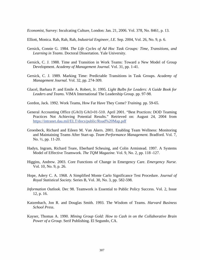
307

Economist, Survey: Inculcating Culture, London: Jan. 21, 2006. Vol. 378, No. 8461, p. 13. Elliott, Monica. Rah, Rah, Rah, Industrial Engineer, I.E. Sep. 2004, Vol. 26, No. 9, p. 6. Gersick, Connie G. 1984. The Life Cycles of Ad Hoc Task Groups: Time, Transitions, and

Learning in Teams. Doctoral Dissertation. Yale University. Gersick, C. J. 1988. Time and Transition in Work Teams: Toward a New Model of Group

Development. Academy of Management Journal. Vol. 31, pp. 1-41. Gersick, C. J. 1989. Marking Time: Predictable Transitions in Task Groups. Academy of

Management Journal. Vol. 32, pp. 274-309. Glacel, Barbara P. and Emile A. Robert, Jr. 1995. Light Bulbs for Leaders: A Guide Book for

Leaders and Teams. VIMA International The Leadership Group. pp. 97-98. Gordon, Jack. 1992. Work Teams, How Far Have They Come? Training. pp. 59-65. General Accounting Office (GAO) GAO-01-510. April 2001. “Best Practices: DOD Teaming

Practices Not Achieving Potential Results.” Retrieved on: August 24, 2004 from https://intranet.dau.mil/ELT/docs/public/Road%20Map.pdf

Groesbeck, Richard and Eileen M. Van Akers. 2001. Enabling Team Wellness: Monitoring

and Maintaining Teams After Start-up. Team Performance Management. Bradford. Vol. 7, No. ½, pp. 11-20.

Hadyn, Ingram, Richard Teare, Eberhard Scheuing, and Colin Armistead. 1997. A Systems

Model of Effective Teamwork. The TQM Magazine. Vol. 9, No. 2, pp. 118 -127. Higgins, Andrew. 2003. Core Functions of Change in Emergency Care. Emergency Nurse.

Vol. 10, No. 9, p. 26. Hope, Adery C. A. 1968. A Simplified Monte Carlo Significance Test Procedure. Journal of

Royal Statistical Society. Series B, Vol. 30, No. 3, pp. 582-598. Information Outlook. Dec 98. Teamwork is Essential to Public Policy Success. Vol. 2, Issue

12, p. 16. Katzenbach, Jon R. and Douglas Smith. 1993. The Wisdom of Teams. Harvard Business

School Press. Kayser, Thomas A. 1990. Mining Group Gold: How to Cash in on the Collaborative Brain

Power of a Group. Serif Publishing. El Segundo, CA.

308

Kinlaw, Dennis C. 1991. Developing Superior Work Teams: Building Quality and the Competitive Edge. Lexington Books. Lexington, MA.

Kline, Paul. 1986. A Handbook of Test Construction: Introduction to Psychometric Design.

Routledge Kegan & Paul Publisher. London, England. Kline, Paul. 1993. The Handbook of Psychological Testing. Routledge Publisher. London,

England. Knight, Pamela J. (2005), Defense Acquisition University, Huntsville, AL,

pjk29@comcast.net. Kruskal, W. H. and W. A. Wallis. 1952. Use of Ranks on One-Criterion Variance Analysis.

Journal of the American Statistical Association. Vol. 47, pp. 583-621. (corrections appear in Vol. 48, pp. 907-911).

Kutzik, Jennifer, S. 2003. It’s EGATS All over Again? Behind the Scenery in Reference

Services. Library Mosaics. Vol. 14, No. 2, p. 14. Lacoursiere, Roy B. 1980. The Life Cycle of Groups. New York Human Sciences Press. New

York, NY. pp. 21, 26, 28, 58, 62. Lau, Debra. 1999. No Rest for The Weary VC: Information Technology Deals Get Done Fast,

or They Get Done by Someone Else. Venture Capital Journal. Wellesley Hills. February 1, 1999.

Leland, Lisa. 2000. Re-Engineering for Efficiency. Graphics Arts Monthly. Vol. 72, No. 4, p.

67. Maples, Mary F. 1988. Group Development: Extending Tuckman’s Theory. Journal For

Specialists in Group Work. Vol. 13. Marks, Michelle A., John E. Mathieu, and Stephen J. A. Zaccaro. 2001. Temporally Based

Framework and Taxonomy of Team Processes, Academy of Management. The Academy of Management Review. Mississippi State. Vol. 26, No. 3, pp. 356-376.

McGrath, Joseph E. 1990. Time Matters in Groups. In J. Galegher, R. E. Kraut, and C. Egido

(Eds.) Intellectual Teamwork: Social and Technical Bases for Collaborative Work. Erlbaum. Hillsdale, NJ.

McGrath, Joseph E. 1991. Time, Interaction, and Performance (TIP) a Theory of Groups.

Small Group Research. Sage Publications. Vol. 22, No. 3, pp. 147-174. McGrew, John F., John G. Bilotta, and Janet M. Deeney. 1999. Software Team Formation and

Decay: Extending the Standard Model for Small Groups. Small Group Research. Vol. 30, No. 2, pp. 209-234.

309

McKinney, Earl H. Jr., James R. Barker, Kevin J. Davis, and Daryl Smith. 2005. How Swift

Starting Action Teams Get Off the Ground: What United Flight 232 and Airline Flight Crews Can Tell Us About Team Communication. Communications Quarterly: McQ. Thousand Oaks. Vol. 19, No. 2, p. 198.

Mennecke, Brian E. and Jeffrey A. Hoffer. 1992. The Implications of Group Development and

History for Group Support System Theory and Practice. Small Group Research. Vol. 23, No. 4, pp. 524-573.

Merton, Robert K. 1957. Social Theory and Social Structure (Rev. ed.) Chicago: Free Press. Metcalfe, Jacqueline and Sarah Garrett. 2005. Team Esteem. Nursing Standard. Vol. 19, No.

21, p. 88. Miller, Diane L. 1997. The Effects of Group Development, Member Characteristics, and

Results on Teamwork Outcomes. Doctoral Dissertation. University of Toronto. Miller, Diane L. 2003. The Stages of Group Development: The Retrospective Study of

Dynamic Team Processes. Canadian Journal of Administrative Sciences. Vol. 17, No. 2. pp. 121-134.

Nixon, Chuck. 2001. Productive Partnerships: Project Teams Work Together. Consulting-

Specifying Engineer. Vol. 30, No. 6, p. 11. Nunnally, Jim C. 1967. Psychometric Theory. McGraw Hill. New York, NY. Offerman, Lynn R. and Rebecca K. Spiros. 2001. The Science and Practice of Team

Development: Improving The Link. Academy of Management Journal 00014273. Vol. 44, No. 2.

Osterman, Paul. 1994. How Common Is Workplace Transformation and Who Adopts It?

Human Relations. Vol. 47, No. 2, pp. 173-188. Perlow, L. A. 2000. Working On Internet Time: An Ethnographic Account. Paper presented at

the annual meeting of the Academy of Management. Toronto. Reid, Hal. 2005. Tsunami Support from MapAction – GIS to the Far Reaches of the World,

Directions Magazine. Retrieved on: 26 Jan 2005 from http://www.directionsmag.com/article.php?article_id=741&trv=1&PHPSESSID=75e2b861e83b140e1de899385111f3d4.

Runkel, Philip J., Marilyn Lawrence, Shirley Oldfied, Mimi Rider, and Candee Clark. 1971.

Stages Of Group Development: An Empirical Test Of Tuckman’s Hypothesis. The Journal of Applied Behavioral Science. Vol. 7, No. 2, pp. 180-193.

310

Sander, Todd. 2001. Striking a Balance Takes Cooperation. American City and County. Vol. 116, No. 5, p. 12.

Siegel, Sidney and N. John Castellan, Jr. 1988. NonParametric Statistics for the Behavioral

Sciences. McGraw Hill Inc. New York, NY. Smith, M. K. 2005. Bruce W. Tuckman—Forming, Storming, Norming, and Performing In

Groups, The Encyclopaedia of Informal Education. Last updated: March 14, 2005. http://www.infed.org/thinkers/tuckman.htm.

Smith, Richard. 1993. No Man is an Island. Financial Management. Vol. 71, No. 8, pp. 63-64. Tarricone, Pina and Joe Luca. 2002. Employees, Teamwork and Social Interdependence—A

Formula for Successful Business. Team Performance Management. Vol. 8, No. 3, pp. 54-59.

Trochim, W. M. 1991. Developing An Evaluation Culture For International Agricultural

Research. In D. R. Lee, S. Kearl, and N. Uphoff (Eds.). Assessing the Impact of International Agricultural Research for Sustainable Development: Preceedings from a Symposium at Cornell University, Ithaca, NY, June 16-19, the Cornell Institute for Food, Agriculture and Development. Ithaca, NY.

Tuckman, B. W. 1965. Developmental Sequence In Small Groups. Psychological Bulletin.

Vol. 63, No. 6, pp. 384-399. Tuckman, B. W. and M. A. C. Jensen. 1977. Stages In Small Group Development revisited.

Group and Organizational Studies. Vol. 2, pp. 410-427. Walters, Keith. 2005. Dream Team. BRW. Vol. 27, No. 40, p. 92. Weinstock, Matthew. GOVEXEC Daily Brief, August 15, 2002. Procure Review Buying

Teams. mweinstock@govexec.com; http://www.govexec.com/top200/02top/s1.htm. Wheelan, S. A. 1994. Group Processes: A Developmental Perspective. Allyn & Bacon: The

Simon & Schuster Education Group. Needham Heights, MA. Wheelan, S. and J. Hochberger. 1996. Validation Studies of the Group Development

Questionnaire. Small Group Research. Vol. 27, No. 1, pp. 143-170. Yancey, Margaret. 1998. CSWT Papers Work Teams: Three Models of Effectiveness, Center

for the Study of Work Teams, University of North Texas, P. O. Box 311280, Denton, TX 76203-1280. Retrieved on 20 August 2004 from http://www.workteams.unt.edu/old/reports/Yancey.html.

311

BIBLIOGRAPHY

Adelson, Joseph. 1975. Feedback and Group Development. Small Group Behavior. Sage Publications. Vol. 6, No. 4.

Agresti, Alan. 1988. A Model for Agreement Between Ratings on Ordinal Scale. Biometrics.

Vol. 44, No. 2, pp. 539-548. Atherton, J. S. 2003. Learning and Teaching: Group Development [Online] UK: Available:

http://www.dmu.ac.uk/~jamesa/teaching/group_development.htm. Accessed: 7 October 2004.

Babad, Elisha Y. and Liora Amir. 1979. Bennis and Shepard’s Theory of Group Development

An Empirical Examination. Small Group Behavior. Vol. November. Bach, G. R. 1954. Intensive Group Psychotherapy. Ronald Press. New York, NY. pp. 268-293. Bales, R. F. and F. L. Strodtbeck. 1951. Phases in Group Problem-Solving. Journal of

Abnormal and Social Psychology. Vol. 46, pp. 485-495. Bales, Robert F. 1950. Interaction Process Analysis: A Method for the Study of Small Groups.

Addison-Wesley. Reading, MA. Bales, Robert F. 1953. The Equilibrium Problem in Small Groups, in T. Parsons, R. F. Bales

and E. A. Shils (eds.), Working Papers in the Theory of Action. Free Press. No. 111-61. Bales, Robert F. 1999. Social Interaction Systems Theory and Measurement. Transaction

Publishers. New Brunsick (USA). Bales, Robert F. and Stephen P. Cohen. 1979. SYMLOG A System for the Multiple Level

Observation of Groups. The Free Press. New York, NY. Barron, M. E. and G. K. Krulee. 1948. Case Study of a Basic Skill Training Group. Journal of

Social Issues. Vol. 4, No. 2, pp. 10-30. Besag, Julian and Peter Clifford. 1989. Generalized Monte Carlo Significance Tests.

Biometrika. Vol. 76, No. 4, pp. 633-642. Bennis, W. G. and H. A. Shepard. 1956. A Theory of Group Development. Human Relations.

Vol. 9, pp. 415-457. Bettenhausen, Kenneth and J. Keith Murnighan. 1985. The Emergence of Norms in

Competitive Decision Making Groups. Administrative Science Quarterly. Vol. 30, pp. 350-372.

Bion, Wildred R. 1961. Experiences in Groups. Basic Books Inc. New York, NY.

312

Blair, Gerard M. 1991. Groups That Work. IEEE Engineering Management Journal. Vol. 1,

No. 5, pp. 219-223. http://www.ee.ed.ac.uk/~gerard/Management/art0.html. Blair, Gerard M. 1997. Laying the Foundations for Effective Teamwork. University of

Edinburgh, Electronics and Electrical Engineering. Edinburgh, Scotland. September 2, 1997. http://www.ee.ed.ac.uk/~gerard/Teaching/art0.html. (Originally published: Engineering Science and Education Journal. Vol. 2, No. 1 (February 1993), pp.15-19).

Blechar, M. 2002. Internet Year Is 3 Months. Gartner Research Group. COM-16-6393. Bradford, Leland P., Jack R. Gibb, and Kenneth D. Benne. 1964. T-Group Theory and

Laboratory Method. John Wiley and Sons. New York, NY. Buffinton, Keith W., Kathryn W. Jablokow, and Kathleen A. Martin. 2002. Project Team

Dynamics and Cognitive Style. Engineering Management Journal. Vol. 14, No. 3, pp. 25-34.

Carew, D. K. and E. Parisi-Carew. 1988. Group Development Stage Analysis: Matching

Leader Behaviors with Team Development. Blanchard Training and Development, Inc. 125 State Place, Escondido, CA 92025.

Chidamdaram, Laku. 1996. Group Development (I): A Review and Synthesis of

Developmental Models. Group Decision and Negotiation. Vol. 6:159; p. 186. Kluwer Academic Publishers.

Cissna, Kenneth N. 1984. Phases in Group Development The Negative Evidence. Small Group

Behavior. Sage Publications. Vol. 15, No. 1, pp. 3-32. Clarkson, Petruska. 1991. Group Imago and the Stages of Group Development. Transactional

Analysis Journal. Vol. 21, No. 1. Coffey, H. S. 1952. Socio and Psyche Group Processes: Integrative Concepts. Journal of

Social Issues. Vol. 8, No. 2, pp. 65-74. Coombs, Clyde H. 1964. A Theory of Data. John Wiley. New York, NY. Cronbach, Lee J. 1951. Coefficient Alpha and the Internal Structure Tests. Psychometrika.

Vol. 16, No. 3. Cronbach, Lee J. 1960. Essentials of Psychological Testing. Harper & Row. New York, NY. Defense Manufacturing Council Review of Office of the Secretary of Defense (OSD)/Service

Oversight Defense Science Board Report on Engineering in the Manufacturing Process (March 1993).

313

Department of Defense Acquisition Workforce Reduction Trends and Impacts—Report No. D-2000-088 (PDF); Date: February 29, 2000. http://www.dodig.osd.mil/audit/reports/fy00/00088sum.htm.

Department of Defense Directive 5000.57, Defense Acquisition University, dated February 8,

2006. http://www.dtic.mil/whs/directives/corres/pdf/i500057_020806/i500057p.pdf. Department of Defense Guide to Integrated Product and Process Development, Version 1.0,

dated February 5, 1996. Issued By: Office of the Under Secretary of Defense (Acquisition and Technology) Washington, DC 20301-3000.

Devine, Dennis J., Laura D. Clayton, Jennifer L. Philips, Benjamin B. Dunford, and Sarah B.

Melner. 1999. Teams in Organizations: Prevalence, Characteristics, and Effectiveness. Small Group Research. Vol. 30, No. 6, pp. 678-711.

DiTrapani, Anthony R. and Jonathan Geithner. 1996. Getting the Most Out of Integrated

Product Teams (IPTs). Center for Naval Analyses, 4401 Ford Avenue, Alexandria, VA; CRM 96-49, May.

Dobrow, Marvin, Peter Miller, Donna Lee Rose, Daniel Thurman, and Toyoko Vassil. 1996. A

Retest of the Reliability of an Instrument and a Test of the Validity of a Model of Group Development. Master’s Thesis. Boston University.

Dunlap, William P., Michael J. Burke, and Kristin Smith-Crowe. 2003. Accurate Tests of

Statistical Significance for rwg and Average Deviation Interrater Agreement Indexes. Journal of Applied Psychology. Vol. 88, No. 2, pp. 356-362.

Dunphy, Dexter C. 1968. Phase, Roles and Myths in Self-Analytics Groups. Journal of

Applied Behavioral Science. Vol. 4, No. 2, pp. 195-225. Dworken, Bari Susan. 1993. A Study of the Developmental Life Cycle of Work Groups: A

Critical Incident Analysis. Doctoral Dissertation. University of Massachusetts. Eakins, Lucia Igou. 1983. Psychometric Properties of the Group Process Questionnaire.

Master’s Thesis. Portland State University. Elrod, Parker David II. 1999. An Empirical Study of the Relationship Between Team

Performance and Team Maturity. Doctoral Dissertation. The University of Alabama in Huntsville.

Evans, N. and D. Jarvis. 1986. The Group Attitude Scale: A Measure of Attraction to Group.

Small Group Behavior. Vol. 17, No. 2, pp. 203-216. Farrell, M. P. 1982. Artists’ Circles and the Development of Artists. Small Group Behavior.

Vol. 13, No. 4, pp. 451-474.

314

Fisher, B. A. 1975. Decision Emergence: Phases In Group Decision Making. Speech Monographs. Vol. 37, pp. 53-66.

Fortune, Juliana L. 2005. The Team Success Questionnaire: A Valid and Reliable Assessment

Tool. Doctoral Dissertation. University of Alabama in Huntsville. Garland, James Allen. 1956. A Reliability Test of an Instrument for Measuring Group

Development. Master’s Thesis. Boston University. Goodman, Paul S., Elizabeth C. Ravlin, and Linda Argote. 1986. Current Thinking About

Groups: Setting the Stage for New Ideas from Designing Effective Work Groups by Paul S. Goodman. Josey-Bass Inc. San Francisco, CA. pp. 1-33.

Greiner, Larry E. 1998. Evolution and Revolution As Organizations Grow. Harvard Business

Review. Vol. May-June, pp. 55-67. Halfhill, T. (In Press). Quantifying The "Softer-Side" Of Management Education: An Example

Using Teamwork Competencies. Journal of Management Education. Halfhill, T. R. and J. W. Huff. 2003. Team Viability: Viable Concept? Roundtable presented at

the annual meeting of the Society for Industrial and Organizational Psychology. Hard, Amy L. 2001. A Behavior-Based Team Training Model: Improving The Ability of

Individuals to Perform in Teams. Master’s Thesis. Siena Heights University. Hare, A. Paul. 1973. Theories of Group Development and Categories For Interaction Analysis.

Small Group Behavior. Sage Publications. Vol. 4, No. 3, pp. 259-305. Hare, Alexander Paul. 1976. Handbook of Small Group Research. The Free Press, New York,

NY. Hare, Alexander Paul, Edgar F. Borgatta, and Robert F. Bales. 1965. Small Groups Studies in

Social Interaction. Alfred A. Knopf Publishers, Inc. Hare, A. P. and D. Naveh. 1984. Conformity and Creativity: Camp David. Small Group

Behavior. Vol. 15, No. 3, pp. 299-318. Heinemann, Gloria and Antonette M. Zeiss. 2002. Team Performance in Health Care. Klewer

Academic/Plenum Publishers, New York, NY. Heinen, J. Stephen and Eugene A. Jacobson. 1976. Model of Task Group Development in

Complex Organizations and a Strategy of Implementation. Academy of Management Journal. Vol. October, pp. 98-111.

Ivancevich, John M. 1974. A Study of a Cognitive Training Program: Trainer Styles and

Group Development. Academy of Management Journal. Vol. 17, No. 3, p. 428.

315

Ivancevich, John M. and J. Timothy McMahon. 1976. Group Development, Trainer Style and

Carry-over Job Satisfaction and Performance. Academy of Management Journal. Vol. 19, No. 3, pp. 395-413.

Jennings, H. H. 1947. Sociometric Differentiation Of The Psychegroup and Sociogroup.

Sociometry. Vol. 10, pp. 71-79. Joey, F. George and Leonard M. Jessup. 1997. Groups Over Time: What are we Really

Studying. International Journal of Human-Computer Studies. Vol. 47, No. 3, pp. 497-511. Jones, J. and W. L. Bearley. 1986. Group Development Assessment (GDA Questionnaire and

Trainer Guide). Organization Design and Development Inc. King of Prussia, PA. Jones, J. 1982. The Team Development Inventory. University Associate. La Jolla, CA. Kazmierski, Stas and Catherine Lilly. 2001. Group Organics Model. OD Practitioner. Vol. 3,

No. 2, pp. 26-33. King, David. 2001. Team Management. CMA Management, Vol. 75, No. 3. Liebowitz, Bernard A. 1972. Method for the Analysis of the Thematic Structures of T Groups.

The Journal of Applied Behavioral Science. Vol. 7, No. 6, pp. 689-709. Lundgren, D. C. 1971. Trainer Style and Patterns of Group Development. The Journal of

Applied Behavioral Science. Vol. 7, No. 6, pp. 689-709. Lundgren, D. C. 1973. Attitudinal and Behavioral Correlates of Emergent Status in Training

Groups. The Journal of Social Psychology. Vol. 90, pp. 141-153. Lyon, J. Michael. 2003. Mentoring of Scientists and Engineers: Dyadic and Formality Effects

on Career Development and Psychosocial Interactions. Doctoral Dissertation. The University of Alabama in Huntsville.

Mallison, Bradford. Group Formation and Development. National Training Laboratories. Mann, R., G. Gibbard, and J. Hartman. 1967. Interpersonal Style and Group Development.

John Wiley. New York, NY. McClure, Bud A. 1998. Putting a New Spin on Groups The Science of Chaos. Lawrence-

Erlbaum Associates Publishers. Mahwah, NJ. pp. 33-58. McGraw, Kenneth O. and S. P. Wong. 1996. Forming Inferences About Some Intraclass

Correlation Coefficients. Psychological Methods. Vol. 1, No. 1, pp. 30-46.

316

McIver, J. P. and E. G. Carmines. 1981. Unidimensional Scaling. Sage Publishing. Thousand Oaks, CA.

Menneke, Brian E. Jeffrey A. Hoffer, and Bayard E. Wynne. 1992. Group Development and

History in GSS Research: A New Research Perspective; IEEE. 0073-1129-1/92. Merriam-Webster’s New Collegiate Dictionary (2003). Modlin, H. C. and M. Faris. 1956. Group Adaptation and Integration In Psychiatric Team

Practice. Psychiatry. Vol. 19, pp. 97-103. Obert, Steven L. 1983. Developmental Patterns of Organizational Task Groups: A Preliminary

Study. Human Relations. Vol. 36, No. 1, pp. 37-52. Philp, H. and D. Dunphy. 1959. Developmental Trends in Small Groups. Sociometry. Vol. 22,

pp. 162-74. Pryweller, Joseph. 2002. Teams Make Short Work Of Time To Market. Plastics News.

Database: Business Source Elite 1042802X. Vol. 14, No. 32. Psathas, G. 1960. Phase Movement and Equilibrium Tendencies in Interaction Process in

Psychotherapy Groups. Sociometry. Vol. 23, pp. 177-194. Rickards, T. 1987. Can Computers help Stimulate Creativity? Training Implications from a

Postgraduate MBA Experience. Management Education and Development. Vol. 18, No. 2, pp. 129-139.

Rickards, Tudor and Susan Moder. 2000. Creative Leadership Processes in Project Team

Development: An Alternative to Tuckman’s Stage Model. British Journal of Management. Vol. 11, pp. 273-283.

Roberts, Alan R. and Phillip C. Withers. 2006. StatistiXL Vol. 1.5, Excel Add In, February

2006. Robertson, Rodney. 2004. An Empirical Study of the Relationship Between The Health of

Project Teams and Their Overall Performance. Doctoral Dissertation. The University of Alabama in Huntsville.

Rodriguez, Margery Regalado. 2001. Tug-O-Warring Toward Change—the Push-Pull

Dynamics Within Organizational Change Efforts. Doctoral Dissertation. The Fielding Graduate Institute.

Schroder, H. M. and O. J. Harvey. 1963. Conceptual Organization and Group Structure, in O.

J. Harvey (ed.), Motivation and Social Interaction. Ronald Press. pp. 134-66.

317

Schutz, W. C. 1958. FIRO: A Three-Dimensional Theory of Interpersonal Behavior. Holt, Rinehart & Winston. pp. 168-188.

Seers, Ason and Steve Woodruff. 1997. Temporal Paces in Task Forces: Group Development

or Deadline Pressure. Journal of Management. Vol. March-April. Shambaugh, Phlip Wells. 1978. The Development of the Small Group. Human Relations.

Vol. 31, No. 3, pp. 283-295. Smith, A. J. 1960. A Developmental Study Of Group Processes. Journal of Genetic

Psychology. Vol. 97, pp. 29-39. Spitzer, Tom. 2001. Balancing Act. Intelligent Enterprise. San Mateo. Vol. 4, No. 5, pp. 26-

34. Stevens, Michael J. 1999. Staffing Work Teams: Development and Validation of a Selection

Test for Teamwork Settings. Journal of Management. Vol. 25, No. 2, pp. 207-228. http://www.findarticles.com/cf_dls/m4256/2_25/54824259/p1/article.jhtml.

Stewart Greg L., Charles C. Manz, and Henry P. Sims, Jr. 1999. Team Work and Group

Dynamics. John Wiley and Sons. New York, NY. Stock, Dorothy. 1964. A Survey of Research on T Groups from Leland P. Bradford, Jack

R.Gibb, and Kenneth D. Benne. T-Group Theory and Laboratory Method. John Wiley and Sons. New York, NY.

Syer, John and Christopher Connolly. 1996. How Teamwork Works the Dynamics of Effective

Team Development. McGraw-Hill. pp. 45-61. Systems Engineering Fundamentals. October 1999. Supplementary text prepared by the

Defense Systems Management College Press. Fort Belvoir, VA. Thelen, H. and W. Dickerman. 1949. Stereotypes and the Growth of Groups. Educational

Leadership. Vol. 6, pp. 309-316. Theodorson, G. A. 1953. Elements In The Progressive Development Of Small Groups. Social

Forces. Vol. 31, pp. 311-320. Utley, Dawn R. 1995. Empirical Validation of Classical Behavioral Concepts with Respect to

Quality Enhancement Implementation in Engineering Organizations. Doctoral Dissertation. The University of Alabama in Huntsville.

Wekselberg, Victor and William C. Goggin. 1997. A Multifaceted Concept of Group Maturity

and Its Measurement and Relationship to Group Performance. Small Group Research. Vol. 28, No. 1, pp. 3-26.

318

Wheelan, Susan A. 1999. Creative Effective Teams. Sage Publications. Thousand Oaks, CA. Whittaker, D. S. 1974. Reactions to Group Situations Test. University Associates. LaJolla,

CA. Wideman, Max. 1998. Project Teamwork, Personality Profiles and the Population at Large: Do

We have Enough of the Right Kind of People? Proceedings of the 29th Annual Project Management Institute Seminar/Symposium. Project Management Institute (Updated presentation, April, 2002.) Long Beach, CA. http://www.maxwideman.com/papers/profiles/intro.htm.

Worchel, Stephen, Sawna Coutant-Sassic, and Michele Grossman. 1992. A Developmental

Approach to Group Dynamics: A Model and Illustrative Research from Group Process and Productivity by Stephen Worchel, Wendy Wood, Jeffrey A. Simpson. Sage Publications. Newbury Park, London. pp. 181-202.

Yalom, Irvin D. 1985. The Theory and Practice of Group Psychotherapy 2nd Edition. Basic

Books Inc. New York, NY. pp. 301-316. Zimmerman, Donald W. 2000. Statistical Significance Levels of Nonparametric Tests Biased

by Heterogeneous Variances of Treatment Groups. The Journal of General Psychology. Vol. 127, No. 4, pp. 354-364.

319

GLOSSARY OF

ACRONYMS AND TERMS

AT&L Acquisition, Technology and Logistics ATO Average Time-of-Occurrence ATS Average Team Score CAT Cooperation and Awareness Threshold CMM Capability Maturity Model CTOD Combining Time-of-Occurrence Data DAG Defense Acquisition Guidebook DAU Defense Acquisition University DCMA Defense Contract Management Agency DoD Department of Defense DoDD Department of Defense Directive F Forming FTO First Time-of-Occurrence GAO General Accounting Office (now known as the Government Accountability

Office) GPQ Group Process Questionnaire H Hypothesis IPPD Integrated Product and Process Development IPT Integrated Product Team IRA Inter-Rater Agreement KW Kruskal-Wallis MOM Measure of Merit MSS Minimum Stage Separation MT Minimum Team (size) MTO Median Time-of-Occurrence N Norming P Performing R Ratio RT Ratio Threshold S Storming SA Sequence Analysis SEI Software Engineering Institute TET Tuckman Error Threshold ToET Total Error Threshold UTD Unconstrained Team Data

320

321

322