small countries and the case for regionalism vs. multilateralism · pdf filesmall countries...
TRANSCRIPT
Small Countries and the Case for Regionalism vs. Multilateralism
Mary E. BurfisherU.S. Department of Agriculture
Sherman Robinson International Food Policy Research Institute
Karen Thierfelder U.S. Naval Academy
TMD DISCUSSION PAPER NO. 54
Trade and Macroeconomics DivisionInternational Food Policy Research Institute
2033 K Street, N.W.Washington, D.C. 20006, U.S.A.
May 2000
TMD Discussion Papers contain preliminary material and research results, and are circulatedprior to a full peer review in order to stimulate discussion and critical comment. It is expected thatmost Dicussion Papers will eventually be published in some other form, and that their content may alsobe revised. This paper is available at http://www.cgiar.org/ifpri/divs/tmd/dp/dp54.htm

Abstract
Much of the debate over whether or not developing countries gain from regional tradeagreements (RTA’s) has focused on two characteristics that are common to developing countries:their relatively high tariffs and their high trade dependencies on one or a few developed tradepartners. In this paper, we address a third common characteristic: their use of distorting domesticpolicies that are closely linked to trade restrictions. We argue that participation in an RTA cancreate pressures for domestic policy reforms. We analyze the case of a small country, Mexico,forming an RTA with two larger countries, the U.S. and Canada, in the North American FreeTrade Agreement (NAFTA). Mexico exhibits all three characteristics of a developing country:relatively high tariffs, a high trade dependency on the U.S., and an extensive and pervasivesystem of farm support that was linked to the restriction of trade. For the analysis, we use a 26-sector, multi-country, computable general equilibrium (CGE) model in which the three single-country models are linked through trade flows, and farm programs are modeled in detail. Wefind that there are welfare gains from trade liberalization in all three countries only whendomestic reforms are in place. Mexico gains from NAFTA only when it also removes domesticdistortions in agriculture. Then, agriculture can generate allocative efficiency gains that are largeenough to offset the terms of trade losses which arise because Mexico has higher initial tariffsthan other RTA members.

Table of Contents
I. Introduction . . . . . . . . . . . . . . . . . . . . . . . . . . . . . . . . . . . . . . . . . . . . . . . . . . . . . . . . . . . . . . 1
II. Recent Literature . . . . . . . . . . . . . . . . . . . . . . . . . . . . . . . . . . . . . . . . . . . . . . . . . . . . . . . . . 2
III. Characteristics of NAFTA Countries . . . . . . . . . . . . . . . . . . . . . . . . . . . . . . . . . . . . . . . . . . 4
A. Country size and trade dependence . . . . . . . . . . . . . . . . . . . . . . . . . . . . . . . . . . . . . . 4
B. Trade restrictions . . . . . . . . . . . . . . . . . . . . . . . . . . . . . . . . . . . . . . . . . . . . . . . . . . . 5
C. Domestic distortions in agriculture . . . . . . . . . . . . . . . . . . . . . . . . . . . . . . . . . . . . . . . 5
IV. The Model . . . . . . . . . . . . . . . . . . . . . . . . . . . . . . . . . . . . . . . . . . . . . . . . . . . . . . . . . . . . . . 6
A. Overview . . . . . . . . . . . . . . . . . . . . . . . . . . . . . . . . . . . . . . . . . . . . . . . . . . . . . . . . . 6
B. Modeling Farm Programs . . . . . . . . . . . . . . . . . . . . . . . . . . . . . . . . . . . . . . . . . . . . . 9
V. Results . . . . . . . . . . . . . . . . . . . . . . . . . . . . . . . . . . . . . . . . . . . . . . . . . . . . . . . . . . . . . . . . 11
VI. Conclusion . . . . . . . . . . . . . . . . . . . . . . . . . . . . . . . . . . . . . . . . . . . . . . . . . . . . . . . . . . . . 13
References . . . . . . . . . . . . . . . . . . . . . . . . . . . . . . . . . . . . . . . . . . . . . . . . . . . . . . . . . . . . . . . . 15
Appendix: Structure of the NAFTA-CGE Model . . . . . . . . . . . . . . . . . . . . . . . . . . . . . . . . . . . 28
Solving the CGE Model . . . . . . . . . . . . . . . . . . . . . . . . . . . . . . . . . . . . . . . . . . . . . . . . 28
Model Specification . . . . . . . . . . . . . . . . . . . . . . . . . . . . . . . . . . . . . . . . . . . . . . . . . . . 33
Model Closure . . . . . . . . . . . . . . . . . . . . . . . . . . . . . . . . . . . . . . . . . . . . . . . . . . . . . . . . . . . . . 41

Our model is an extension of the CGE modeling undertaken at the USDA, which began1
with a single-country model of the United States to analyze the effects of changes in agriculturalpolicies and exogenous shocks on U.S. agriculture ( Robinson, Kilkenny, and Hanson, 1990). See Kilkenny and Robinson (1990) and Kilkenny (1991) for an extension of that model to includedetailed U.S. farm programs. See Hinojosa and Robinson (1991) and Burfisher, Robinson, andThierfelder (1992) for earlier versions of the U.S.-Mexico model used in this paper.
1
I. Introduction
Much of the debate over whether or not developing countries gain from regional tradeagreements (RTA’s) has focused on two characteristics that are common to developing countries:their relatively high tariffs, and their high trade dependencies on one or a few developed tradepartners. In this paper, we address a third common characteristic: their use of distortingdomestic policies that are closely linked to trade restrictions. We argue that participation in anRTA can create pressures for domestic policy reforms. Because many domestic policies,particularly in agriculture, insulate producers from changing market prices, these domesticreforms can be crucial for the efficiency gains from trade liberalization to be realized. Furthermore, the pressure for domestic reform is stronger the higher the developing country’strade dependence on its RTA partner. Since an RTA can force domestic adjustments that will benecessary for global trade liberalization, it can be a building bloc towards multilateralism.
In this paper, we analyze the case of a small country, Mexico, forming an RTA with twolarger countries, the U.S. and Canada, in the North American Free Trade Agreement (NAFTA). Mexico exhibits all three characteristics of a developing country: relatively high tariffs, a hightrade dependency on the U.S., and an extensive and pervasive system of farm support that waslinked to the restriction of trade. For the analysis, we use a 26-sector, multi-country, computablegeneral equilibrium (CGE) model in which the three single-country models are linked throughtrade flows, and farm programs are modeled in detail. We simulate NAFTA under two regimes:1
First, we assume the farm programs which restricted supply responses in the three countriesremained in place when NAFTA was implemented. Next, we assume NAFTA occurs in anenvironment with reformed, largely nondistorting farm programs evident in all three countries in1997. While domestic budgetary and political pressures were important motivations for thedomestic farm program reforms in all three countries over the past decade, we show that tradepolicy reforms also created pressure for domestic policy changes. We calculate the budget costsof maintaining distortionary programs in the presence of open regional trade and show that theRTA would have dramatically increased the cost of distortionary domestic programs in Mexico. The comparison of the two scenarios illustrates the effects domestic policy distortions have onwelfare changes following an RTA.
We find that trade creation exceeds trade diversion under NAFTA, whether or notdomestic reforms have occurred. However, there are greater gains when domestic farm program
In contrast, when the union partner is the supplier facing constant costs, an RTA2
improves welfare in the liberalizing country. It benefits from the price reduction and still collectstariff revenue from the countries excluded from the union. There is only trade creation from theRTA. As Panagariya (1996) notes, this case is even better than multilateral tariff elimination dueto the tariff revenue collected. However, he argues it is usually the case that the rest of the world,not the union partner, faces constant costs while union members face increasing costs. Whilethere will be trade creation for some commodities, the majority of goods will come from a partnerwith increasing costs — trade diversion will dominate in most RTAs.
2
reforms have been adopted. Furthermore, there are welfare gains from trade liberalization in allthree countries only when domestic reforms are in place. For Mexico, domestic farm programreforms linked to NAFTA are critical: agriculture can now generate allocative efficiency gains thatare large enough to offset the terms of trade losses which arise because Mexico has higher initialtariffs than other RTA members. Mexico gains from NAFTA only when it also removesdomestic distortions in agriculture.
The next section reviews recent literature on the effects of RTAs versus multilateralism ondeveloping economies. Section three describes trade policies, domestic farm programs and tradedependencies in NAFTA countries. Section four presents the main features of our NAFTA-CGEmodel, emphasizing our specification of agricultural policies. Section five presents the empiricalresults, and the final section presents conclusions.
II. Recent Literature
Much of the debate over the benefits of regional trade agreements (RTA’s) versusmultilateral free trade addresses trade creation and trade diversion effects of an RTA. Bhagwatiand Panagariya (1996) and Panagariya (1998, 1996) make the case for multilateralism by arguingthat small countries lose unambiguously from an RTA and gain unambiguously frommultilateralism. Because RTAs give preferential treatment to member countries, they divert tradefrom non-member, least-cost suppliers. To illustrate the trade diversion effects of an RTA, theypresent Viner's model of a customs union in which two countries remove bilateral tariffs. Whenthe rest of the world is the least cost supplier and faces constant costs, an RTA with the supplierwho faces increasing costs can only divert trade. The liberalizing country loses because it2
foregoes tariff revenue from the new union member but does not face a lower internal price forthe imported good, since the rest of the world determines its market price. In this framework, thelarger the trade partner’s share of total imports, the bigger the tariff revenue loss when an RTA isformed. Similarly, the trade partner who initially has higher tariffs loses from an RTA becausemore tariff revenue is redistributed away from it. Since developing countries often have hightrade dependencies and high tariffs, Bhagwati and Panagariya argue that they will lose from anRTA. They make the case for multilateralism, arguing that the small country must gain whendomestic producers compete at the world price, and any tariff revenue transferred to the RTA

Schiff (1996) also discusses country size and the welfare impacts of an FTA. Like3
Panagariya, he argues that the smaller a country’s imports from its partner, the smaller thewelfare losses of foregone tariff revenue.
This calculation uses aggregate trade and tariff numbers — the changes in total U.S.4
exports to Mexico and the average wage.
See also Winters (1996) for a discussion of the theory with models that allow both trade5
creation and trade diversion. De Rosa (1998) provides a balanced survey of theoretical modelsthat allow for both trade creation and diversion when an RTA is formed with a partner facingeither constant or increasing cost.
3
partner will be returned to domestic consumers.3
As an example of the damage an RTA does to a developing country, Panagariya (1997)calculates welfare losses as high as $3.26 billion for Mexico from NAFTA. When making thiscalculation, he assumes that the rest of the world is the least cost supplier with a horizontal exportsupply curve and that the U.S. has increasing costs so its supply curve is upward sloping. SinceMexico had higher initial tariffs than the U.S., its loss of tariff revenue exceeds its gains frompreferential access to the U.S. market (foregone tariff revenue in the U.S.).4
De Melo et al. (1993) note that the case of pure trade diversion, while unambiguouslywelfare-worsening, is too extreme a model to characterize actual RTAs. They present a more5
balanced view of the welfare effects of an RTA in an analytical model in which integration bothcreates and diverts trade. In this case, the country which lowers its barriers against a trade partnerfaces a new domestic price which is lower than the tariff-inclusive mark-up over the constant costsupplier (the rest of the world), but higher than the free trade price. The welfare effects on thetariff-reducing country are ambiguous: it loses because it has diverted all imports from the lowestcost supplier, but it benefits because total imports have increased. De Melo and others note that,in this environment: (1) the higher the initial tariff on a given sector, the larger the benefits and thesmaller the costs of an RTA; (2) the lower the post-RTA tariff on non-union countries, the lesslikely that the lower-priced goods of the latter will be displaced; and (3) the greater thecomplementarity in import demands between the union partner, the greater the gains from anRTA. The latter point suggests that there are large gains from an RTA between developed anddeveloping countries — such as the U.S. and Mexico — which have different factorendowments. Determining the net welfare impact of an RTA in this model is an empirical issue.
Robinson and Thierfelder (1999) survey the empirical literature in which multi-countryCGE models have been used to analyze the impact of regional trade agreements. The multi-country CGE models differ widely in terms of country and commodity coverage, assumedmarket structure, policy detail, and specification of macroeconomic closure. In spite of thesedifferences, surveys of these models support two general conclusions about the empirical effects
They incorporate two domestic distortions — rent-seeking activities associated with6
import quotas and sector-specific minimum wages which induce rural-urban migration — in ageneral equilibrium model of the Philippines.
Anderson uses a CGE model with nine developing countries and 15 agricultural sectors.7
He simulates world price changes due to the Uruguay round, from Goldin and van derMensbrugghe (1995), in two versions of the base model — one with and the other withoutdistortions. Anderson and Tyers (1993) perform similar simulations — world price shocks in amodel with and without domestic distortions in agriculture — in a partial equilibrium framework. They also find that domestic distortions are at least as important to domestic welfare as are tradeprices.
4
of regional trade agreements: (1) in aggregate, trade creation is always much larger than tradediversion; and (2) welfare — measured in terms of real GDP or equivalent variation — increasesfor member countries.
In addition to issues relating to trade diversion and tariff revenue losses, developingcountries also have domestic distortions which affect the welfare gains from an RTA. Clarete andWhalley (1988) discuss the links between domestic distortions and trade reform in a small openeconomy. They find significant interactions between trade and domestic policies and that the6
social cost of trade distortions are approximately doubled when distortions are included. Asthey conclude, “The lesson would seem to be that these interactions need to be considered morefully in numerical economic policy analysis for developing countries.” (p. 358).
Moving in that direction, Anderson (1997) evaluates the interaction between trade reformunder the Uruguay Round and domestic distortions in agriculture in developing countries.He introduces the anticipated agricultural price increases in a general equilibrium model withdomestic distortions in agriculture. 7
Like Anderson, we consider the effects of trade liberalization with and without domesticintervention in agriculture. However, we model agricultural policies in more detail, not just asexogenous price wedges. This lets us discuss domestic agricultural policies that are directly linkedto trade restrictions. In this framework, trade liberalization, as under an RTA, increases the costof domestic support, creating pressure for reform.
III. Characteristics of NAFTA Countries
A. Country size and trade dependence
GDP data indicate that Mexico is much smaller than the U.S., its primary trade partner.Mexico accounts for 5.1 percent of NAFTA GDP, while the U.S. accounts for 87.5%. LikeMexico, Canada is relatively small in the region, accounting for only 7.4% of NAFTA GDP.

In our NAFTA simulations, we maintain U.S. sugar import restrictions for Canada; we8
eliminate the U.S. sugar quota against Mexico.
See Burfisher, Robinson, and Thierfelder (1998) for a more detailed discussion of the9
changes in domestic farm programs in each NAFTA country.
5
Data on bilateral trade flows reveal a lopsided dependency between the U.S. and Mexico.Mexico is heavily dependent on the U.S. for trade (table 1). In 1993, 81.2% of its total exportswent to the U.S. The U.S. was an even bigger market for Mexico’s agriculture as 94.2% of itsagricultural exports went to the U.S. In contrast, the U.S. sent 7.4% of its total exports and 7.1%of its agricultural exports to Mexico. Similarly on the import side, Mexico is heavily dependenton the U.S., which accounts for 80.0% of Mexico’s imports. In agriculture Mexico’sdependence is not as strong, with 61.0% of its imports coming from the U.S. The U.S. relies onMexico for only 5.1% of its imports, however the dependence is stronger in agriculture for whichMexico supplies 32.7% of the U.S. total.
B. Trade restrictions
In general, pre-NAFTA tariff rates among the U.S. and Canada are low, while those ofMexico are relatively high. In table 2, we show the combined tariff rate equivalent of appliedtariffs and import quotas that were in place in 1993, the model base year. Mexico has the highesttariffs and tariff equivalent of quotas among NAFTA countries, with a trade weighted average of7.9%. In contrast, the trade weighted averages for the U.S. and Canada are 2.9% and 1.9%respectively. There is considerable intersectoral variation in tariff rates in all three countries.Mexico has high trade restrictions in wheat (67%) and corn (90.4%), two crops which the U.S.supports through endogenous input subsidies to maintain a fixed output price. One implicationis that under NAFTA increased Mexican demand for U.S. wheat and corn will reduce the cost ofsuch price supports. U.S. protection rates are high for sugar manufacturing (70%), reflecting theU.S. sugar quota.8
C. Domestic distortions in agriculture
Domestic agricultural programs in all three NAFTA countries have undergonefundamental change since the CUSTA and NAFTA agreements were first initiated (table 3). Ingeneral, these reforms have both lowered support levels and “decoupled” support by makingpayments independent from farmers’ production decisions or market conditions. 9
In the U.S., farm program reforms began in the mid-1980's with the introduction ofincreased planting flexibility and fixed base program acreage (USDA, 1996). In 1996, the U.S.adopted the Federal Agriculture Improvement and Reform (FAIR) Act, whose main effect was to replace the crop-linked, deficiency payments/supply management program with a program of temporary “contract” payments based on land acreage enrolled in the former deficiency
6
payments program. The payments were capped at about $36 billion over 1996-2002, andscheduled to decline over the 7-year program.
Canada introduced its new generation of farm programs in 1991 under the Farm IncomeProtection Act (FIPA). Among the reforms was the elimination of grain freight subsidies byAugust, 1995. Subsidies were replaced with voluntary revenue insurance programs to whichproducers and the federal and provincial governments contribute. The Gross Revenue InsuranceProgram (GRIP) has already been discontinued due to its high costs. The Net IncomeStabilization Account (NISA) extends farm income risk management support to all grains,oilseeds, and some horticulture. The government provides matching grants to farmers’contributions to savings accounts. Savings earn relatively high, subsidized rates of return andfarmers may withdraw funds during years of lower than average income. Canada continues tosupport poultry, dairy, and eggs through supply management programs. These programs rely onproduction and import quotas to maintain farm prices for these commodities at levels that arebased on the costs of production. Because the effectiveness of these programs requires traderestrictions, Canada has exempted these three sectors from free trade under NAFTA. Butter andskim milk prices are additionally supported through marketing board purchases, and exportsubsidies financed through levies on producers. Direct payments to dairy producers were phasedout in 1996.
Mexican agricultural policy reforms began in the late 1980's. In 1988, tariffs were sharplylowered following Mexico’s accession to the GATT, and most import quotas were converted totariffs. However, import licensing remained an important instrument for price support --particularly for corn, a staple crop produced by Mexico’s large subsistence farm sector. Beginning in 1991, Mexico began to lower agricultural input subsidies, and the reduce thepervasive role of the government in purchasing, storing and distributing agricultural commodities. Subsidies to corn and wheat millers were reduced, and most retail food price controls wereeliminated. Guaranteed producer prices and government purchases were continued only for cornand beans. In 1993, in anticipation of NAFTA, Mexico adopted the PROCAMPO program. PROCAMPO is a 15-year, direct payments program that compensates producers for the loss ofinput subsidies, price support, and import protection. It was designed to provide transitional,decoupled income support to farmers, while allowing Mexico’s agriculture to undergo structuralchange in response to market conditions. In 1996, Mexico announced the Alliance for theCountryside (Alianza para al Campo), a major initiative to improve agricultural productivity. Alianza is an umbrella grouping that includes PROCAMPO and other programs.
IV. The Model
A. Overview
The NAFTA-CGE model is a 26-sector, multi-country, CGE model of the U.S., Canada,

The countries can also be linked through international migration flows. To focus on the10
welfare effects of an RTA in a second-best environment, we chose not to include migrationflows. See Burfisher, Robinson, and Thierfelder (1992) for a discussion of US-Mexico tradewhen migration can occur.
Robinson (1989) surveys CGE models applied to developing countries. Shoven and11
Whalley (1984) survey models of developed countries. The theoretical properties of this familyof trade-focused CGE models are discussed in Devarajan, Lewis, and Robinson (1990).
We assume an elasticity of substitution between land types in Mexico of 0.8 in all12
sectors.
This treatment, whereby Mexican rural income in the migration equation includes both13
wages and a share of land income, differs from that in Robinson, et al. (1993). This specificationis closer to that of Levy and van Wijnbergen (1994), who describe migration as a function ofincome or utility differentials.
7
and Mexico in which the three single-country models are linked through trade flows. For the10
purpose of describing the model, it is useful to distinguish between the individual “country”models and the multi-region model system as whole, which determines how the individualcountry models interact. When the model is actually used, the within country and betweencountry relationships are solved for simultaneously.
Each country CGE model follows closely what has become a standard theoreticalspecification for trade-focused CGE models. In addition to 26 sectors – including eight farm11
and nine food processing – each country model has seven factors of production – four labortypes, two land types, and capital. Land is disaggregated into irrigated and dryland in Mexico. Each crop uses both land types in production and it is assumed that the land types are poorsubstitutes. Both irrigated and dryland are perfectly mobile across crops. In the United States,12
each crop is grown using one of two possible land types. One land type is used to produce eitherfruits/vegetables, cotton, or other agricultural production. The second land type is assumed to beperfectly mobile among wheat, corn, other feed grains, and oilseeds production. Capital ismobile across sectors. Labor is mobile across sectors, but it is segmented into four laborcategories. There is some labor mobility between labor categories due to labor migration. Weassume full employment and constant factor supplies.
Mexican rural workers can migrate to urban unskilled labor markets in Mexico. Thedomestic factor supplies incorporate the migrant labor flows. Migration is assumed to depend onwage differentials. In equilibrium, migration maintains a fixed wage differential between ruraland urban unskilled labor markets in Mexico. The average wage, upon which labor bases itsmigration decision, includes labor income plus a share of the dryland income for rural workers. 13
Migration flows generated by the CGE model refer to changes from a base flow of zero. Theyshould be viewed as additional migration flows due to the policy change, adding to (or reducing)

8
current flows.
For each sector, the model specifies production, consumption and trade equations. Output supply is given by constant elasticity of substitution (CES) value added productionfunctions, while intermediate inputs are demanded in fixed proportions. Producers are assumedto maximize profits, implying that each factor is demanded so that marginal revenue productequals marginal cost. However, factors do not receive a uniform wage or “rental” (in the case ofcapital) across sectors; instead, we include sectoral factor market distortions that fix the ratio ofthe sectoral return to a factor relative to the economy-wide average return for that factor. Thesefactor market distortions can be interpreted as productivity differences based on sectoraldifferences in value added shares to each input.
The single aggregate household in each economy has a Cobb-Douglas expenditurefunction, consistent with optimization of a Cobb-Douglas utility function. Sectoral householdconsumption is a fixed share of household income. Real investment and governmentconsumption by sector are constant in the model simulations. Consumers demand a compositeof the imported and domestic variety of each good.
Sectoral export-supply and import-demand functions are specified for each country. Incommon with other CGE models (both single and multi-country), the NAFTA-CGE modelspecifies that goods produced in different countries are imperfect substitutes. At the sectorallevel, in each country, demanders differentiate goods by country of origin and exportersdifferentiate goods by destination market. When modeling import demands, the Almost IdealDemand System (AIDS) specification is adopted. This specification allows import expenditureelasticities to be different from one and also allows cross-country substitution elasticities to varyfor different pairs of countries. Exports are supplied according to a CET function betweendomestic sales and total exports, and allocation between export and domestic markets occurs inorder to maximize revenue from total sales. The rest of the world is modeled simply as a supplierof imports to and demander of exports from the three NAFTA countries. Production activities inthe rest of the world are not explicitly modeled; instead, this region is assumed to have flatexport-supply curves and downward-sloping aggregate import-demand curves. With thisstructure, we can incorporate the key assumption of Bhagwati and Panagariya that supply fromRTA partner countries is less elastic than that from the rest of world.
In common with other CGE models, the model only determines relative prices and theabsolute price level must be set exogenously. In our model, the aggregate consumer price indexin each sub-region is set exogenously, defining the numeraire. The advantage of this choice isthat solution wages and incomes are in real terms. The solution exchange rates in the sub-regionsare also in real terms, and can be seen as equilibrium price-level-deflated (PLD) exchange rates,

De Melo and Robinson (1989) and Devarajan, Lewis, and Robinson (1993) discuss the14
role of the real exchange rate in this class of model. We fix the exchange rate for the rest ofworld, thereby defining the international numeraire.
9
using the country consumer price indices as deflators. World prices are converted into domestic14
currency using the exchange rate, including any tax or tariff components. Cross-trade priceconsistency is imposed, so that the world price of Mexico’s exports to the U.S. are the same asthe world price of the U.S.’s imports from Mexico.
At the macro economic level, all income from production goes to the single householdwhich pays taxes and consumes based on fixed expenditure shares. The government collectstaxes, administers transfer payments and has a fixed real expenditure on goods and services. Thegovernment budget deficit is endogenous. Total savings of households, the government andforeign capital must equal investment, which is fixed. The household savings rate is endogenousto insure that savings equals investment. The current account is constant and the exchange ratevaries.
Each country model traces the circular flow of income from producers, through factorpayments, to households, government, and investors, and finally back to demand for goods inproduct markets. The country models incorporate tariffs which flow to the government, and non-tariff revenues which go to the private sector. Each economy is also modeled as having a numberof domestic market distortions. There are sectorally differentiated indirect taxes, as well ashousehold and corporate income taxes. Production distortions in agriculture are modeled indetail, as described below. When we simulate NAFTA, we maintain domestic distortions insectors other than agriculture.
B. Modeling Farm Programs
We model agricultural trade and domestic farm programs explicitly as either pricewedges, which affect output and labor migration decisions; lump-sum income transfers; or asswitching regimes which respond to price or output targets. The wedges and transfers are eitherspecified exogenously or determined endogenously, depending on the institutional characteristicsof the program being modeled. See table 4 for a summary of the various programs, the variablesthey affect and the countries in which they apply.
Many of the 1993 policies are “coupled” in that they influence producers’ decisions. These policies affect the producer's value added price, the payment to primary factors. It iscalculated as the unit value of production net of indirect taxes and payments to intermediategoods. Government subsidies are calculated per unit of output and are added to the value addedprice as the producer incentive equivalent (PIE) (equation 1, table 5a). A positive PIE increasesthe payment to factors, pulling resources into the subsidized sector and increasing output.

Alternatively, the participation rate can be made endogenous, and changes in deficiency15
payment expenditures would result from both changes in the deficiency payment and fromchanges in base acreage.
To model this, we maintain an upper bound on the output level in these sectors. When16
there is pressure for output to expand beyond the constraint, the marginal factor productivitydeclines; resources become more expensive, eliminating the incentive to expand output.
Both the supply and price management policies are modeled as switching regimes using17
the PATH solver in GAMS.
10
The components of the producer incentive equivalent vary by sector and by country. InCanada and Mexico, it consists of exogenous input subsidies whose rate varies by sector (seetable 3). The PIE for Mexican corn millers also includes endogenous payments under theGuaranteed Price Program. The Mexican government fixes the price of corn and compensatesthe corn millers for the artificially high price of inputs. In the United States, the PIE consists of the deficiency payments which are determined endogenously, and are not treated as fixed advalorem wedges. Following Kilkenny (1991), and Kilkenny and Robinson (1990), we model theU.S. deficiency payment as per unit of output as the difference between a fixed target price andthe market price. We calculate the initial unit value of the deficiency payment from data on totalgovernment expenditure on deficiency payments (including direct deficiency payments andmarketing loan deficiency payments), base output, and participation rates. The unit value of thedeficiency payment is a component of the producer incentive equivalent (equation 2, table 5a). We fix the eligible production at the base year levels. The total payment a farm receives is the15
payment rate multiplied by eligible base production. Planting flexibility introduced under the1990 Farm Bill is captured by treating 50% of deficiency payments as direct payments, or incometransfers.
In all three countries, direct payments are modeled as income transfers to the household,and are decoupled from producers’ decision-making. In Mexico, the direct payment alsosupplements the rural wage, thereby influencing the rural migration decision. In the U.S., thedirect payment is assumed to be capitalized in returns to land. In Canada, NISA payments areassumed to be nondistorting household income transfers.
Canada restricts the supply of livestock and poultry. Producers minimize cost subject to aconstraint on the level of output (equation 6, table 5a). Similarly, Canada also maintains a fixed16
price for dairy manufacturing (equation 7, table 5a). We impose a lower bound on the outputprice. When there is pressure for the price to fall below the target price, the governmentsubsidizes exports to bolster the price to farmers.17
All countries impose tariffs and quotas on farm and food processing sectors (equations 4and 5, table 5a). These border policies indirectly affect the producer value added price through

Since we start from different base models, we must compare absolute, not percent,18
changes across scenarios.
The U.S. maintains its import quota on processed sugar from Canada and dairy19
manufactured goods from Canada; Mexico and Canada retain bilateral restrictions on eachothers’ imports of dairy manufactured goods and poultry.
11
their effect on the price of domestic output. Since we treat imports as imperfect substitutes fordomestic goods, we insulate the domestic price from the full effect of border price shocks. Tariffs and quotas raise the price of imports, increasing demand for the domestically producedvariety, and raising its price. Since the producer price is a weighted average of the prices ofoutput sold on the domestic market and in each export market, it, too, will increase. Tariffs aremeasured as an ad valorem rate. They increase the domestic price of the imported good relativeto its world price.
In the model, we assume endogenous ad valorem tariff equivalents of quotas. The initialrates are calculated as the wedge between the world price and the domestic price, adjusted fortransport costs and any tariffs that are used in combination with the quota. In the model, thesetariff equivalent rates adjust to maintain a specified level of imports.
Under NAFTA, import quotas are converted to tariff rate quotas (TRQ). Under thissystem, a specified volume of a commodity may enter at low or zero duty, and quantities abovethat level are taxed at a higher rate. In the model, TRQ rates are invoked endogenously whenimports exceed a specified quantity threshold (equation 8, table 5a).
For each country, net farm program expenditure is computed by summing governmentexpenditure and revenues arising from the various programs. In the model, it is included in totalgovernment fiscal expenditure and any increase in the net farm program expenditure will increasethe government budget deficit.
V. Results
We simulate NAFTA under two regimes: First, we assume the farm programs whichrestricted supply responses in the three countries remained in place when NAFTA wasimplemented, at 1993 levels of program expenditure. Next, we assume NAFTA occurs in anenvironment with the reformed, largely nondistorting farm programs evident in all three countriesin 1997, at 1997 levels of program expenditure. In both scenarios, we model NAFTA as the18
removal of bilateral trade barriers among all three countries, with the exceptions of some sectorsas specified by the Agreement. 19
In all three countries, NAFTA has a greater effect on agriculture under the new farmprograms than under pre-NAFTA farm programs. Production changes by a bigger absolute

12
amount in each country, with the biggest changes occurring in the U.S. and Mexico, countrieswhich insulated agriculture from price shocks with pre-NAFTA farm programs. Under both oldand new programs, NAFTA has a greater impact on Mexican agriculture than on U.S. andCanadian farm sectors, reflecting Mexico’s greater trade dependence on its North Americanpartners and higher pre-NAFTA trade barriers.
Another indication of NAFTA’s impact is the change in factor employment defined as the number of workers, acres of land, and value of capital stock initially employed in agriculturethat must find new employment, in agriculture or elsewhere, after changes in agricultural policies(table 6). In Mexico, employment effects of NAFTA are substantially greater under the newfarm programs than the old – 1.2 percent of the agricultural labor force must find newemployment under old programs while 4.5% must change sectors under new programs. Thesame pattern holds for the U.S., but the changes are less extreme with a 0.1 percent change inlabor employment under the old programs and a 0.2 percent change under the new programs. InCanada, labor adjustment to NAFTA is marginally greater under its new program than under itspre-NAFTA farm support program (0.379 percent vs. 0.385 percent).
Under both old and new farm programs, Mexico’s terms of trade decline because ofNAFTA. Mexico’s import barriers were higher than those of its North American partners,causing Mexico’s imports to increase more than its exports as those barriers were lifted. Someanalysts have cited the deterioration in Mexico’s terms of trade due to NAFTA as an argumentagainst regional trade agreements (Bhagwati and Panagariya, 1996). We find that Mexicoexperiences a welfare loss only when there are distorting domestic policies in place that preventan efficient reallocation of resources in response to trade reforms. Similarly, in the U.S., theflexibility introduced by farm program reform leads to larger welfare gains under NAFTA (tables7 and 8). Under decoupled farm programs, resources can move more easily into sectors thatbecome more profitable under free trade and out of sectors that face import competition. ForMexico, the problem is exacerbated by the dramatic increase in farm program expenses underfree trade and distorting policies. There is an increase in lump sum taxes on the consumer,reducing welfare as real disposable income declined.
Under both old and new programs, trade creation dominates trade diversion. Tradeexpansion (defined as the increase in total exports) is the highest for the U.S. and the lowest forMexico. Furthermore, farm program reforms within NAFTA also benefit members’ trade withnonmembers. There is less absolute trade diversion for the U.S. and Canada and Mexico’s tradewith non-member countries increases more under new farm programs.
At the sectoral level, output changes following NAFTA illustrate the interaction betweendomestic and trade policies. Under Mexico’s former, guaranteed price program, producers andconsumers faced fixed prices for corn. Input subsidies to corn millers compensated them forpurchasing corn at the artificially high, guaranteed price. To reduce the costs of its corn pricesupport program, Mexico restricted corn imports; the tariff equivalent of the quota was 90.4percent in 1993. With this program in place, corn milling production would have increased

Indeed, Mexico initiated its reform program, PROCAMPO, in October 1993, before20
NAFTA went into effect.
13
substantially under NAFTA to maintain the domestic price of corn which also faced downwardpressure from cheaper imported corn. Mexican corn output would have risen slightly, despiteelimination of high trade barriers to corn. To maintain its guaranteed price for corn underNAFTA, Mexico’s farm program expenditures would have increased by 140 percent. Such adramatic increase in program costs demonstrates why Mexico needed to restructure its farmprogram support in a free trade environment. 20
In contrast, without price supports for corn, Mexico’s corn production declines followingNAFTA as consumers substitute cheaper imported corn for the domestic variety. Corn millingoutput increases by a smaller amount as producers are responding only to cheaper imported corn,not an increased subsidy to maintain demand for domestic corn. Other agricultural sectorsbenefit in Mexico. Fruit and vegetables expands more as resources are released from cornproduction. Likewise wheat does not contract as much. This affects the U.S., whose wheatexports to Mexico do not expand as much under NAFTA with the new programs compared tounder NAFTA with the old programs.
In the U.S., the interaction between domestic and trade policies is less dramatic than inMexico, because U.S. price support programs did not rely on tariffs to help support the domesticprice. The U.S. had endogenous deficiency payments to maintain fixed output prices for wheat,corn, feedgrains, and oilseeds. As in Mexico, these programs insulated producers from increasedcompetition due to NAFTA. However, for the U.S., NAFTA increased demand for cropsformerly supported with deficiency payments, particularly corn and wheat. In the scenario withNAFTA under the old farm programs, U.S. farm program expenditures actually declined slightlyby 0.5%..
VI. Conclusion
Mexico, when it considered joining NAFTA, had characteristics typical of a smalldeveloping country: (1) relatively high tariffs; (2) a high trade dependency on its RTA partner;and (3) extensive domestic distortions in agriculture. According to some theoretical models, itsrelatively high tariffs and trade dependence meant welfare losses under NAFTA. We find thatdomestic distortions contribute to net welfare losses because they insulate agriculture and preventthe efficient reallocation of domestic resources in response to changing market signals. They alsorequire a lump sum tax increase on consumers in order to maintain high farm prices whenborders are opened. However, when domestic reforms accompany NAFTA, Mexico experiences
This is in contrast to Panagariya (1997), who does not consider domestic distortions21
when he calculates the welfare losses of NAFTA for Mexico. Instead, he bases his analysis onthe tariff revenue lost and trade diversion with no trade creation.
14
a welfare gain from the RTA. While Mexico still experiences terms of trade losses, its larger21
efficiency gains now lead to a net welfare gain under NAFTA. Furthermore, we find that tradecreation dominates trade diversion with and without domestic policy reforms. There is greatertrade expansion when domestic distortions are removed.
Similar to Mexico, many developing countries maintain distorting domestic farmprograms whose effectiveness depends on trade restrictions. We find that high tradedependencies and high tariffs — other characteristics of developing countries — create pressurefor domestic reform following the formation of an RTA. Given the current emphasis on reducingdistortions in agriculture in the Uruguay round and future multilateral negotiations, our resultssuggest that an RTA can be a building bloc, not a stumbling bloc, to multilateralism.
15
References
Anderson, James E. (1997). “The Uruguay Round and Welfare in Some Distorted AgriculturalEconomies,” NBER Working Paper No. 5932.
Anderson, Kym and Rod Tyers (1993). “More on Welfare Gains to Developing Countries fromLiberalizing World Food Trade,” Journal of Agricultural Economics, Vol 44, no. 2, pp.189-204.
Bhagwati, Jagdish (1993). “Regionalism and Multilateralism: an Overview,” in De Melo, Jaimeand Arvind Panagariya (eds.), New Dimensions in Regional Integration. Cambridge:Cambridge University Press.
Bhagwati, Jagdish and Anne Krueger (1995). The Dangerous Drift to Preferential TradeAgreements. Washington, D.C.: AEI Press.
Bhagwati J. and Arvind Panagariya (1996). “Preferential Trading Areas and Multilateralism --Strangers, Friends, or Foes?” in, The Economics of Preferential Trade Agreements,editedby Jagdish Bhagwati and Arvind Panagariya. Washington, D.C.: AEI Press.
Brooke, Anthony, David Kendrick, and Alexander Meeraus (1988). GAMS: A User's Guide. Redwood City, CA: The Scientific Press.
Burfisher, Mary E., Sherman Robinson and Karen Thierfelder (1998). “Farm Policy Reforms andHarmonization in the NAFTA,” in Regional Trade Agreements and U.S. Agricultureedited by Mary E. Burfisher and Elizabeth A. Jones. Washington, D.C.: U.S. Departmentof Agriculture, Agriculture Economic Report Number 771.
Burfisher Mary E., Sherman Robinson and Karen Thierfelder (1992). “Agricultural and FoodPolicies in a United States-Mexico Free Trade Area,” North American Journal ofEconomics and Finance, Vol 3, no. 2, pp. 117-139.
Clarete, Ramon L. and John Whalley (1988). “Interactions between Trade Policies and DomesticDistortions in a Small Open Developing Economy,” Journal of International Economics,Vol. 24, pp. 345-358.
DeRosa, Dean A. (1998). “Regional Integration Arrangements: Static Economic Theory,Quantitative Findings, and Policy Guidelines,” Policy Research Working Paper 2007.Washington, D.C.: The World Bank.
Devarajan, Shantayanan, Jeffrey D. Lewis and Sherman Robinson (1990). “Policy Lessons fromTrade-Focused, Two-Sector Models.” Journal of Policy Modeling. Vol. 12, pp. 625-657.

16
Devarajan, Shantayanan, Jeffrey D. Lewis, and Sherman Robinson (1993). “External Shocks,Purchasing Power Parity, and the Equilibrium Real Exchange Rate.” World BankEconomic Review, Vol. 7., No. 1 (January), pp. 45-63.
Goldin, Ian and Dominique van der Mensbrugghe (1996). “Assessing Agricultural Tarifficationunder the Uruguay Round,” in The Uruguay Round and the Developing Countries,edited by Will Martin and L. Alan Winters. Cambridge: Cambridge University Press.
Green, Richard and Julian M. Alston (1990). “Elasticities in AIDS Models.” American Journalof Agricultural Economics. Vol. 72, no. 2 (May), pp. 442-445.
Hinojosa-Ojeda, Raul and Sherman Robinson (1991). “Alternative Scenarios of U.S.-MexicoIntegration: A Computable General Equilibrium Approach,” Giannini FoundationWorking Paper No. 609, University of California, Berkeley.
Kilkenny, Maureen (1991). “Computable General Equilibrium Modeling of Agricultural Policies:Documentation of the 30-Sector FPGE GAMS Model of the United Sates,” Report No.AGES 9125, Economic Research Service. Washington, DC: U.S. Department ofAgriculture.
Kilkenny, Maureen and Sherman Robinson (1990). “Computable General Equilibrium Analysisof Agricultural Liberalization: Factor Mobility and Macro Closure,” Journal of PolicyModeling, Vol 12., pp. 527-556.
Levy Santiago and Sveder van Wijnbergen (1994). “Agriculture in the Mexico-U.S. Free TradeAgreement: A General Equilibrium Analysis,” in Modeling Trade Policy: AppliedGeneral Equilibrium Assessments of North American Free Trade, edited by Joseph F.Francois and Clinton R. Shiells. Cambridge: Cambridge University Press.
de Melo, Jaime and Sherman Robinson (1989). “Product Differentiation and the Treatment ofForeign Trade in Computable General Equilibrium Models of Small Economies.” Journal of International Economics. Vol. 27, no. 1-2 (August), pp. 47-67.
Panagariya, Arvind (1998). “The Regionalism Debate: An Overview,” Center for InternationalEconomics, Department of Economics, University of Maryland at College Park, Workingpaper No. 40.
Panagariya, Arvind (1997). “An Empirical Estimate of Static Welfare Losses to Mexico fromNAFTA”, unpublished mimeo, Center for International Economics, University ofMaryland, College Park.
Panagariya, Arvind (1996). “The Free Trade Area of the Americas: Good for Latin America?” TheWorld Economy, Vol. 19, no 5. pp. 485 - 516.

17
Robinson, Sherman (1989). “Multisectoral Models,” in Handbook of Development Economics,edited by Hollis Chenery and T.N. Srinivasan. Amsterdam: New Holland.
Robinson, Sherman, Mary E. Burfisher, Raul Hinojosa-Ojeda, and Karen Thierfelder (1993).“Agricultural Policies and Migration in a U.S.-Mexico Free Trade Area: A ComputableGeneral Equilibrium Analysis,” Journal of Policy Modeling, Vol 15 nos. 5&6, pp. 673-701.
Robinson, Sherman, Maureen Kilkenny and Kenneth Hanson (1990). “The USDA/ERSComputable General Equilibrium Model of the United States. Report No. AGES 9040. Economic Research Service. Washington, DC: U.S. Department of Agriculture.
Robinson, Sherman, Mary Soule, and Silvia Weyerbrock (1991). “Import Demand Functions,Trade Volume, and Terms-of-Trade Effects in Multi-Country Trade Models.” Unpublished manuscript, Department of Agricultural and Resource Economics,University of California at Berkeley.
Robinson, Sherman and Karen Thierfelder (1999). “Trade Liberalization and RegionalIntegration: The Search for Large Numbers,” International Food Policy Research Institute,Trade and Macroeconomics Division, Working Paper No. 34.
Schiff, Maurice (1996). “Small Is Beautiful: Preferential Trade Agreements and the Impact ofCountry Size, Market Share, Efficiency and Trade Policy,” Policy Research WorkingPaper 1668. Washington, D.C.: The World Bank.
Shoven, John B. and John Whalley (1984). “Applied General-Equilibrium Models of Taxationand International Trade.” Journal of Economic Literature. Vol. 22, no. 3 (September),pp. 1007-1051
U.S. Department of Agriculture, Economic Research Service (1996). Provisions of the FederalAgriculture Improvement and Reform Act of 1996. Agriculture Information Bulletin No.729.
Winters, L. Alan (1996). “Regionalism versus Multilateralism,” Policy Research Working Paper1687. Washington, D.C.: The World Bank.

18
Table 1 — Trade dependencies among NAFTA countries, 1993
Imports from partner (as a percent of total) Exports to partner (as a percent of total)
U.S. Canada Mexico Rest of World U.S. Canada Mexico Rest of World
United States
Total 17.40 5.11 77.48 17.61 7.44 74.95
Agriculture 44.87 32.70 22.43 16.52 7.11 76.37
Canada
Total 70.93 0.91 28.16 78.58 0.53 20.89
Agriculture 75.54 1.16 23.30 39.52 2.13 58.35
Mexico
Total 79.88 1.38 18.74 81.23 3.25 15.52
Agriculture 61.02 5.70 33.29 94.21 2.65 3.14

19
Table 2 — Tariff and tariff equivalent of quota rates, 1993
U.S. Canada Mexico
Poultry 0.49 0.30 10.58
Livestock 0.82 0.56 15.00
Wheat 2.47 0.00 67.00
Corn 0.15 0.23 90.38
Feed grain 0.15 0.00 9.07
Fruits & vegetables 4.55 0.95 16.30
Oilseeds 0.00 0.00 7.30
Other agriculture 1.60 0.64 8.79
Forestry & fisheries 0.26 0.47 11.78
Meat 9.60 3.04 19.70
Dairy manufacturing 6.78 12.30 89.60
Sugar manufacturing 70.40 4.93 15.00
Prepared fruits & vegetables 5.26 7.00 20.00
Wheat milling 1.06 2.84 17.41
Feed milling 0.10 1.43 8.64
Corn milling 0.50 2.84 11.07
Oil milling 1.08 7.10 20.10
Miscellaneous food processing 5.50 9.30 30.10
Light manufacturing 8.96 3.44 9.76
Oil 0.55 0.08 5.79
Intermediates 4.06 0.60 6.04
Fertilizer 3.51 1.84 8.02
Consumer durables 2.42 1.78 9.12
Capital goods 2.56 1.46 7.81
Services 0.00 0.00 0.00
Trade weighted average 2.92 1.91 7.91
Source: World Trade Organization, tariff data base; various Attache Reports, Foreign AgriculturalService, USDA; tariff equivalent of quotas are calculated by authors from PSE data, and InternationalTrade Commission (1990). Import quotas converted to tariff rate quotas in 1995.

20
Table 3 — Producer incentive equivalent of agricultural distortions, 1993U.S Canada Mexico
1993 1997 1993 1997 1993 1997
subsidy rate per unit of output
Poultry 0.21 0.00 0.32 0.10 7.30 1.37
Livestock 0.45 0.00 0.25 0.56 3.59 0.64
Wheat 14.09 3.55 0.43 0.52 2.68 1.29
Corn 6.11 0.65 0.18 0.09 2.56 1.05
Feedgrain 17.96 2.08 0.11 0.24 2.15 1.94
Oilseeds 2.18 0.96 0.17 0.16 2.67 0.37
Other agriculture 7.54 0.11 0.10 0.10 0.09 0.05
Meat manufacturing 0.00 0.33 0.00 0.00 0.00 0.00
Dairy manufacturing 0.01 0.30 2.65 0.06 5.84 5.12
Sugar manufacturing 0.67 0.34 0.00 0.00 1.14 0.35
Wheat milling 0.00 0.00 0.00 0.00 1.78 0.00
Feed milling 0.00 0.00 0.00 0.00 4.21 0.00
Corn milling 0.00 0.00 0.00 0.00 14.56 12.15
Note: Producer incentive equivalent refers to subsidy expenditure relative to producer price. Source: OECD, “Producer and Consumer Subsidy Equivalents,” electronic data base, 1998.

21
Table 4 — How policies are modeled
Countries and sectors Impact Instrument
Endogenous Exogenous
Deficiency Payments U.S. : wheat, corn, feed grain & other PVA, value added price DEFPAYagriculture
Input subsidies Mexico: livestock, wheat, corn, feed PVA, value added price insubgrain, oil seeds, other agriculture & dairymanufacturing
Canada: poultry, livestock, wheat,corn, feed grain, oil seeds, & dairymanufacturing
Guaranteed price Mexico: corn prices are fixed, subsidy to PX, output price for the sector in which PSUBU, per corn millers prices are guaranteed & PVA, value added unit subsidy to
price in the sector which uses the fixed the processorprice commodity as an input
Tariff rate quotas U.S.: sugar and dairy manufacturing PWM, world import price TRQagainst Canada and Rest of World
Mexico: dairy manufacturing and poultryagainst Canada
Tariffs U.S.: all sectors PWM, world import price tm
Mexico: all sectors
Canada: all sectors

Countries and sectors Impact Instrument
Endogenous Exogenous
22
Quotas U.S.: sugar manufacturing, dairy PWM, world import price TM2manufacturing, & meat (treated asexogenous in base model and eliminatedfor partner countries in NAFTA)
Mexico: wheat, corn, & dairymanufacturing (treated as exogenous inbase model and eliminated for partnercountries in NAFTA)
Indirect taxes U.S.: all sectors PD, domestic sales price itax
Canada: all sectors except prepared fruitsand vegetables
Value added tax Mexico: all sectors PVA, value added price vatr,
Export subsidies Canada: wheat, feed grain and oilseeds PE, domestic export price te0
Supply management Canada: livestock & poultry X, output level is constant SCALE,payment tovalue added
Price management Canada: dairy manufacturing PX, output price is constant TE, exportsubsidy
Crop and revenue Canada: grains and oilseeds PVA, value added price insinsurance U.S.: grains and oilseeds
Direct payments U.S., Mexico, and Canada YH, household income dirpay

PVAi,k ' PXi,k & Ój IOj,i,k % PIEi,k
PIEi,k 'DEFPAYi,k
Xi,k
% insubi,k % PSUBUi,k
DEFPAYi,k ' X̄Pi,k @ ( ¯TPi,k & PXi,k )
PMi,k,cty1 ' PWMi,k,cty1 @EXRk @
(1 % tmi,k,cty1 % TM2i,k,cty1 % TRQi,k,cty1 )
TARIFFk,cty1 ' jitmi,k,cty1 @Mi,k,cty1 @PWMi,k,cty1 @EXRk %
jiTRQi,k,cty1 @(Mi,k,cty1 & M0i,k,cty1 ) @PWMi,k,cty1 @EXRk
Xi,k # X̄i,k SCALEI,K # 1
PXi,k $ P̄Xi,k TEi,k $ 0
Mi,k,cty1 # M̄i,k,cty1 TRQi,k,cty1 $ 0
EXPSUBk ' ji,cty1( te0i,k,cty1 % TEi,k,cty1 ) @
PWEi,k,cty1 @Ei,k,cty1 @EXRk
23
Table 5a — Policy equations
# Equation Comple- Descriptionmentarity constraint
1 Value added price
2 Producerincentiveequavalent (PIE)
3 Deficiencypayment
4 Import price
5 Tariff revenuewith snapbackprovision
6 Supplymanagement
7 Price management
8 Tariff rate quota
9 Export subsidy
Note: the subscripts i refers to sectors; k refers to NAFTA countries; and cty1 refers to NAFTA countries and therest of the world; a bar over a variable indicates a fixed level of that variable.

24
Table 5b — Model variables
DEFPAY Deficiency payment by sectori,k
E Exports of good i from country k to country cty1i,k,cty1
EXPSUB Export subsidy paid by country kk
EXR Exchange rate by country k
IO Input output table: amount of good i used to make one unit of good j, by countryi,j,k
M Imports of good i in country k, from country cty1i,k,cty1
PIE Producer incentive equivalent of price support programs for good i, in country k;i,k
measured per unit of output
PREM Quota rents for good i in country ki,k
PVA Value added price of good i in country ki,k
PWE World price of exports from country cty1 in country k for good ii,k,cty1
PWM World price of imports from country cty1 in country k for good ii,k,cty1
PX Output price of good i in country ki,k
SCALE Constraint on marginal factor productivity in production of good i in country ki,k
TE Export subsidy on good i from country k to country cty1, to maintain price ofi,k,cty1
commodity i in country k (price management policy)
TM2 Tariff equivalent of the quota on imports of good i from country cty1, in country k i,k,cty1
TP Target output price of good i in country ki,k
TRQ Tariff rate quotas on country k’s imports of good i from country cty1,i,k,cty1
X Output of good i in country ki,k
Parameters
insub Input subsidy per unit of output of good i in country ki,k
te0 Export subsidy per unit of export on good i from country k to country cty1i,k,cty1
tm Tariff rate per unit of import on country k’s import of good i from country cty1i,k,ct

25
Table 6 — Factor market adjustment following NAFTA (percent change)
NAFTA and 1993 NAFTA and 1997 PoliciesPolicies
U.S.
Labor 0.124 0.156
Capital 0.033 0.045
Land 0.070 0.046
Canada
Labor 0.379 0.385
Capital 2.203 2.208
Land 0.039 0.040
Mexico
Labor 1.151 4.520
Capital 2.600 3.540
Land 4.845 4.174
Note: Percent change in factor employment refers to number of workers, land, or capital thatleave any farm sector due to NAFTA, relative to base level of agricultural employment. Theymay be reemployed in other farm or nonfarm sectors.

26
Table 7 – Aggregate results, NAFTA and 1993 policies
Real GDP Real Absorption Farm Program Expenditure Terms of Trade
percent change from base
U.S. 0.01 0.01 -0.49 0.56
Canada 0.01 0.11 -0.07 0.37
Mexico 0.03 -0.11 140.21 -0.92
Trade Trade Creation Trade Diversion WelfareExpansion b
billion U.S. dollars
U.S. 5.80 6.27 -0.47 0.34
Canada 2.29 5.67 -3.37 0.57
Mexico 0.81 0.41 0.40 -1.02
Welfare is calculated as equivalent variation; in the format reported here, a positive number is a welfare gain.a
Trade expansion is defined as the increase in exports from the base for each country; trade creation is the increaseb
in exports to countries in NAFTA; trade diversion is the change in exports to countries outside NAFTA (the rest ofworld).

27
Table 8 – Aggregate results, NAFTA and 1997 policies
Real GDP Real Absorption Farm Program Terms of TradeExpenditure
percent change from base
U.S. 0.01 0.01 0.03 0.58
Canada 0.01 0.11 -0.25 0.37
Mexico 0.26 0.10 -0.42 -1.03
Trade Expansion Trade Creation Trade Diversion Welfareb
billion U.S. dollars
U.S. 5.84 6.47 -0.63 0.43
Canada 2.30 5.67 -3.37 0.57
Mexico 0.90 0.42 0.48 0.34
Welfare is calculated as equivalent variation; in the format reported here, a positive number is a welfare gain.a
Trade expansion is defined as the increase in exports from the base for each country; trade creation is the increaseb
in exports to countries in NAFTA; trade diversion is the change in exports to countries outside NAFTA (the rest ofworld).

PINDCON ' ki
PQpwtc i
i
GAMS is suiitable for solving linear, non-linear, or mixed integer programming22
problems as well. For a thorough introduction to model-building in GAMS, see Brooke,Kendrick, and Meeraus (1988).
28
Appendix: Structure of the NAFTA-CGE Model
Solving the CGE Model
The CGE model presented here has been developed and solved using a package called theGeneral Algebraic Modeling System (or GAMS). GAMS is designed to make complex22
mathematical models easier to construct and understand. We use it to solve a large, fullydetermined, non-linear CGE model in which the number of equations equals the number ofvariables. GAMS has become a powerful tool for modelers because of two related developmentsof the last several years. First, the increasing power and availability of personal computers allowsevery modeler to have desktop access to computational resources that were once available onlyon mainframe computers. Second, the development of packaged software such as GAMS, tosolve complex mathematical or statistical problems has permitted modelers to return theirattention to economics.
To a great extent, the GAMS representation of model equations is easily read as standardalgebraic notation. Subscripts indicating countries, sectors, or factors appear in parentheses [Xijbecomes X(i,j)], and a few special symbols are used to indicate algebraic operations [Ó becomesSUM, Ð becomes PROD]. For example, the Cobb-Douglas consumer price index equation:
is represented in GAMS as:PINDCON = PROD(i, PQ(i)**pwtc(i,k))
where PROD stands for the product operator Ð, the i at the left of the parenthetic expression isthe sectoral index over which summation occurs, and the two asterisks (**) indicateexponentiation.
The “$” introduces a conditional “if” statement in an algebraic statement. For example,PM(i,k,cty1)$imi(i,k,cty1) = xxx will carry out the expression shown for all PM(i,k,cty1) thatbelong to the set imi(i,k,cty1); in other words, calculate an import price for all sectors in whichthere are imports.
Tables 1 and 2 list the regional, sectoral, and factor classifications used in the model, aswell as identifying the sectoral subsets that are needed in the equations of the model. Table 3contains the parameter definitions used in the CGE model equations. Table 4 contains thevariables that appear in the model.

29
COUNTRIES AND REGIONSCTY1,CTY2 Universe US United States CA Canada
MX MexicoRT Rest of World
K(cty1), L(cty1) Countries US United States CA Canada
MX Mexico
SECTORS AND GROUPINGSI,J, Sectors of production POULTRY Poultry
LVSTK LivestockWHEAT WheatCORN CornFEEDGRN Feed GrainsFRTVEG Fruits & VegetablesOILSEED OilseedsOTHAG Other AgricultureFOR-FISH Forestry & FisheryFOOD Processed FoodMEAT Processed MeatsDAIRYMFG Dairy ManufacturingSUGARMFG Sugar ManufacturingFVPREPS Prepared Fruits & VegetablesWHTMILL Wheat MillingFEEDMILL Feed MillingCORNMILL Corn MillingOILMILL Oil MillingMISCFOOD Miscellaneous FoodsLMFG Light ManufacturingOL OilINT Intermediate GoodsFERT FertilizerCD Consumer DurablesKG Capital GoodsSE Services
ik(i) Capital and intermediates (OL, INT, KG)oil(i) Oil sector (OL)noil(i) Non-oil sectorsiag(i) Agricultural sectors (POULTRY, LVSTK, WHEAT, CORN, FEEDGRN, FRTVEG, OILSEED, OTHAG) iagn(i) Non-agricultural sectorsipr(i) Processing sectors (MEAT, DAIRYMFG, SUGARMFG, FVPREPS, WHTMILL, FEEDMILL, CORNMILL, OILMILL,
MISCFOOD)iprn(i) Non-processing sectorsim(i,k) Import sectorsimn(i,k) Non-import sectorsie(i,k) Export sectorsien(i,k) Non-export sectorsimi(i,k,cty1) Bilateral imports in base dataiei(i,k,cty1) Bilateral exports in base dataie1(i,k) Aggregate CET export sectorsie2(i,k) Competitive export sectors (WHEAT.CA, WHEAT.US)iec(i,k) Sectors with second-level export CET (All sectors in this version of the model)iecn(i,k) Sectors with second-level competitive sectorsied(i,k) Sectors with export demand from RTiedn(i,k) Not ied (All sectors in this version of the model)iedw(i,k) Setors with export RT-demand belonging to an aggregate curveisnap(i,k,cty1) Sectors with snap-back provisions (SUGARMFG.US.CA, SUGARMFG.US.RT, DAIRYMFG.US.CA, DAIRMFG.US.RT,
DIARYMFG.MX.CA, POULTRY.MX.CA)SMGMT(i,k) Sectors with supply management (LVSTK.CA, POULTRY.CA) NSMGMT(i,k) Non-supply management sectorsPMGMT(i,k) Price management sectors (DAIRYMFG.CA)NPMGMT(i,k) Non-price management sectorsDPAY(i,k) Endogenous deficiency payment sectors (WHEAT.US, CORN.US, FEEDGRN.US, OTHAG.US)NDPAY(i,k) Non-deficiency payment sectorsFXP(i,k) Fixed price sectors (CORN.MX)PS(i,k) Producer Subsidy Sectors (CORNMILL.MX)NPS(i,k) Non-Producer Subsidy sectors
Table 1: Regional and Sectoral in the NAFTA-CGE Model
30
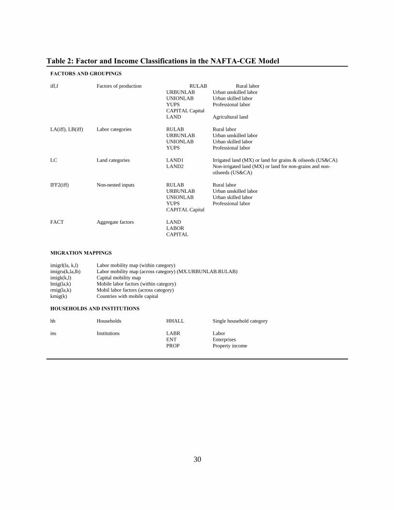
FACTORS AND GROUPINGS
iff,f Factors of production RULAB Rural laborURBUNLAB Urban unskilled laborUNIONLAB Urban skilled laborYUPS Professional laborCAPITAL CapitalLAND Agricultural land
LA(iff), LB(iff) Labor categories RULAB Rural laborURBUNLAB Urban unskilled laborUNIONLAB Urban skilled laborYUPS Professional labor
LC Land categories LAND1 Irrigated land (MX) or land for grains & oilseeds (US&CA)LAND2 Non-irrigated land (MX) or land for non-grains and non-
oilseeds (US&CA)
IFF2(iff) Non-nested inputs RULAB Rural laborURBUNLAB Urban unskilled laborUNIONLAB Urban skilled laborYUPS Professional laborCAPITAL Capital
FACT Aggregate factors LANDLABORCAPITAL
MIGRATION MAPPINGS
imigrl(la, k,l) Labor mobility map (within category)imigru(k,la,lb) Labor mobility map (across category) (MX.URBUNLAB.RULAB)imigk(k,l) Capital mobility maplmig(la,k) Mobile labor factors (within category)rmig(la,k) Mobil labor factors (across category)kmig(k) Countries with mobile capital
HOUSEHOLDS AND INSTITUTIONS
hh Households HHALL Single household category
ins Institutions LABR LaborENT EnterprisesPROP Property income
Table 2: Factor and Income Classifications in the NAFTA-CGE Model

31
Model ParametersCLES(i,hh,k) Household consumption sharesENTR(k) Enterprise income tax rateGLES(i,k) Government expenditure sharesHHTR(hh,k) Household income tax rateIO(i,j,k) Input-output coefficientsITAX(i,k) Indirect tax ratesMPS(hh,k) Savings propensities by householdsPVAB0(i,k) Base-year value added pricePWTC(i,k) Consumer price index weights (PQ)PWTS(i,k) Consumer price index weights (PD)PWTX(i,k) Consumer price index weights (PX)SPREM(i,k) Share of premium revenue to the governmentSSTR(iff,k) Factor payment tax ratesTC(i,k) Consumption tax ratesTE0(i,k) Tax rates on exportsTHSH(hh,k) Household transfer income sharesTM(i,k,cty1) Tariff rates on importsTMREAL(i,k,cty1) Real tariff rates on imports for real GDP calculationsVATR(i,k) Value added tax rateXP0(i,k) Initial quantity of output under deficiency payments programZSHR(i,k) Investment demand shares
Production and trade function parametersAC(i,k) Armington function shift parameterAD(i,k) Cobb-Douglas production function shift parameterAD2(i,k) CES production function shift parameterAE(i,k) CET export composition function shift parameter ALPHA(i,iff,k) Cobb-Douglas factor share parameterALPHA2(i,iff,k) CES factor share parameterAT(i,k) CET function shift parameterDELTA(i,k,cty1) Armington function share parameterGAMMA(i,k,cty1) CET export composition function share parametersGAMMAK(i,k) CET function share parameterRHOE(i,k) CET export composition function exponentRHOP(i,k) CES production function exponentRHOT(i,k) CET function exponent
Nested land function parametersALC(i,k) CES land composite function shift parameterALPHALC(i,lc,k) CES land share parameterRHOL(I,K) CES land aggregate exponentSIGMALC(i,k) Elasticity of substitution in land composite
Parameters for farm programsDIRPAY(k) Direct paymentsINSUB(i,k) Input subsidy rate per unit of output
Parameters for AIDS import demand functionsAMQ(i,k,cty1) Share parameter in AIDS functionAQ(i,k) Constant in translog price index AQS(i,k) Constant in Stone price indexBETAQ(i,k,cty1) Coefficient in AIDS functionELASTPQ(i,k,cty1) Translog own price elasticity of dmeandELASTPQ2(i,k,cty1) Stone own price elasticity of demandELASTSQ(i,k,cty1,cty2) Translog elasticity of substitutionELASTSQ2(i,k,cty1,cty2) Stone elasticity of substutitionGAMMAQ(i,k,cty1,cty2) Price parameter in AIDS functionSMQ0(i,k,cty1) Base year import value shareSUMYQ(i,k) Weighted sum of income elasticities
Table 3: Parameters in the NAFTA-CGE Model

32
Price blockEXR(k) Exchange rateGDPDEF(k) GDP deflatorPD(i,k) Domestic pricesPDA(i,k) Domestic prices net of indirect taxesPE(i,k,cty1) Domestic price of exportsPEK(i,k) Average domestic price of exportsPINDCON(k) Consumer price indexPINDEX(k) Output price indexPINDOM(k) Domestic price indexPM(i,k,CTY1) Domestic price of imported goodsPQ(i,k) Price of composite goodsPREM(i,k) Premium income from import rationingPVA(i,k) Value added price including subsidiesPVAB(i,k) Value added price net of subsidiesPWE(i,cty1,cty2) World price of exportsPWERAT(i,k) Ratio of world export pricesPWEFX(i) Benchmark world export pricePWM(i,cty1,cty2) World price of importsPX(i,k) Average output priceTE(i,k) Export subsidiesTM2(i,k,cty1) Import premium ratesTM3(i,k,cty1) Snapback tariffs
Production blockD(i,k) Domestic sales of domestic outputE(i,cty1,cty2) Bilateral exportsEK(i,k) Aggregate sectoral exportssINT(i,k) Intermediate demandM(i,cty1,cty2) Bilateral importsQ(i,k) Composite goods supplySCALE(i,k) Output multiplierSMQ(i,k,cty1) Import value share in total sectoral
demandX(i,k) Domestic output
Factor blockAGDIST(k) Adjustment to restrict agricultural
capitalAVWF(iff,k) Average wage with current weightsFDSC(i,iff,k) Factor demand by sectorFS(iff,k) Factor supplyFSAG(k) Agricultural capital stockFT(k) Factor tax rateWF(iff,k) Average factor priceWFDIST(i,iff,k) Factor differentialYFCTR(iff,k) Factor income
Land blockLFDSC(i.lc,k) Land demand by sectorFSL(lc,k) Land supplyWLC(lc,k) Average land type priceWLDIST(i.lc,k) Land differential
Farm programsDEFPAY(i,k) Deficiency paymentsFPE(k) Total farm program expendituresPIE(i,k) Producer incentive equivalentPSUBU(i,k) Producer subsidy rateTP(i,k) Target price
Migration blockMIGK(K) Capital migration flowsMIGL(la,k) Labor migration flows (within category)MIGRU(la,k) Labor migration flows (across category)WGDFL(la,k,lb,l) Wage differentialsWGDFK(k,l) Rental differentials
Income and expenditure blockCDD(i,k) Private consumption demandDST(i,k) Inventory investment demandENTSAV(k) Enterprise savingsENTAX(k) Enterprise taxesENTT(k) Government transfers to enterprisesESR(k) Enterprise savings rateEXPSUB(k) Export subsidy paymentFBAL(K) Current account balanceFBOR(k) Foreign borrowing by governmentFKAP(k) Foreign capital flow to enterprisesFSAV(k,cty1) Bilateral net foreign savingsFSAVE(k)Foreign savingsFTAX(k) Factor taxesGD(i,k) Government demand by sectorGDPVA(k) Nominal expenditure GDPGDTOT(k) Government real consumptionGOVSAV(k) Government savingsGOVREV(k) Government revenueHHT(k) Government transfer to householdsHSAV(k) Aggregate household savingsHTAX(k) Household taxesID(i,k) Investment demand (by sector of origin)INDTAX(k) Indirect tax revenueREMIT(k) Remittance income to householdsRGDP(k) Real GDPSSTAX(k)Factor taxesTARIFF(k,cty1) Tariff revenueVATAX(k) Value added taxesYH(hh,k) Household incomeYINST(ins,k) Institutional incomeZFIX(k) Fixed aggregate real investmentZTOT(k) Aggregate nominal investment
WelfareCDH(i,hh,k) Consumption by household and
commodityUTIL(hh,k) Utility by householdEV(hh,k) Equivalent variationYN(hh,k) New spending on consumer goods for EV
calculation
Table 4: Variables in the NAFTA CGE model

For Mexico, each farm product can be produced using irrigated and non-irrigated land. 23
For the U.S. and Canada, land is restricted to two subsets of farm sectors: grains and oilseedsuse one type of land while all other agricultural sectors use another type of land.
33
(1) X(i,k) =AD2(i,k)* ( SUM(iff$FDSC0(i,iff,k), ALPHA2(i,iff,k)*FDSC(i,iff,k)**(-RHOP(i,k))) )**(-1/RHOP(i,k)) ;
(2) (1-ft(i,iff2,k))*WF(iff,k)*WFDIST(i,iff,k) = SCALE(i,k)*(1 - vatr(i,k))*pva(i,k)*AD2(i,k)*( SUM(f$FDSC0(i,f,k), ALPHA2(i,f,k)*FDSC(i,f,k)**(-RHOP(i,k))) )
**((-1/RHOP(i,k)) - 1)*ALPHA2(i,iff,k)*FDSC(i,iff,k)**(-RHOP(i,k)-1);
(3) FDSC(i,"land",k) =E= ALC(i,k)*( SUM(lc$LFDSC0(i,lc,k), ALPHALC(i,lc,k)*LFDSC(i,lc,k)**(-RHOL(i,k))) )**(-1/RHOL(i,k)) ;
(4) WLC(lc,k)*WLDIST(i,lc,k) = SCALE(i,k)*(1 - vatr(i,k))*PVA(i,k)*SAD(i,k)*SAD2(i,k)*AD2(i,k)* (SUM(f$FDSC0(i,f,k), ALPHA2(i,f,k)*FDSC(i,f,k)** (-RHOP(i,k))) )**((-1/RHOP(i,k)) - 1)* ALPHA2(i,"land",k)*FDSC(i,"land",k)**(-RHOP(i,k) -1)* ALC(i,k)*(SUM(sct$LFDSC0(i,sct,k), ALPHALC(i,sct,k)*LFDSC(i,sct,k) **(-RHOL(i,k)) ) )**((-1/RHOL(i,k)) -1)*ALPHALC(i,lc,k) *LFDSC(i,lc,k)**(-RHOL(i,k) -1) ;
(5) WFDIST(iag,"capital",k) = AGDIST(k)*WFDIST0(iag,"capital",k) ; (6) INT(i,k) = SUM(j, IO(i,j,k)*X(j,k));
Table 5: Quantity Equations in the NAFTA-CGE Model
Model Specification
There are 26 sectors for each country in the model; to focus on agricultural policies andtrade, there are 9 farm sectors and 10 food processing sectors in the model. There are eightfactors of production – rural labor, urban unskilled labor, urban skilled labor, professional labor,irrigated and non-irrigated land, agricultural capital and capital used in other sectors. The output-supply and input-demand equations are shown in Table 5. Output is produced according to aconstant elasticity of substitution, CES, production function of the primary factors (equation 1),with intermediate inputs demanded in fixed proportions (equation6). There is a CES aggregationof irrigated and non-irrigated land (equation 3). Producers are assumed to maximize profits,23
implying that each factor is demanded such that marginal product equals marginal cost (equation2 for all factors except land and equation 4 for land types). In each economy, factors are notassumed to receive a uniform wage or “rental” (in the case of capital) across sectors. “Factormarket distortion” parameters (the WFDIST (WLDIST) that appears in equation 2 (equation 4))are imposted that fix the ratio of the sectoral return to a factor relative to the economy-wideaverage return for that factor. Agricultural capital is restricted to farm sectors. Rather than createtwo types of capital inputs, we introduce the variable, AGDIST(k) which allows the payment toagricultural capital to adjust to meet the constraint that the supply of agricultural capital is

34
(7) PM(i,k,cty1) = PWM(i,k,cty1)*EXR(k) *(1 + TM(i,k,cty1) + TM2(i,k,cty1) + TM3(i,k,cty1) ) ;
(8) PE(iei,k,cty1) = PWE(iei,k,cty1)* (1 + te0(iei,k) + TE(iei,k))*EXR(k) ; (9) PE(ie2,k,cty1) = PD(i,k);
(10) PWE(i,cty1,cty2) =E= PWM(i,cty2,cty1) ;
(11) PEK(i,k) * EK(i,k) =E= SUM(cty1$pt(k,cty1), PE(i,k,cty1) * E(i,k,cty1) ) ; (12) PDA(i,k) =E= (1-itax(i,k))*PD(i,k) ;
(13) PQ(i,k)*Q(i,k) =E= PD(i,k)*D(i,k) +SUM(cty1$imi(i,k,cty1), (PM(i,k,cty1)*M(i,k,cty1))) ; (14) PX(i,k)*X(i,k) =E= PDA(i,k)*D(i,k) +SUM(cty1$iei(i,k,cty1), (PE(i,k,cty1)*E(i,k,cty1))) ; (15) PINDCON(k) =E= PROD(i$pwtc(i,k), PQ(i,k)**pwtc(i,k)) ;
(16) PVA(i,k) =E= PX(i,k) - SUM(j,IO(j,i,k)*PQ(j,k)) + PIE(i,k);
(17) PVAB(i,k) =E= (1.0-ITAX(i,k))*PD(i,k)*D(i,k)/X(i,k)+ (SUM(cty1, PE(i,k,cty1)*E(i,k,cty1) ))/X(i,k)-SUM(j,IO(j,i,k)*PQ(j,k)) ;
Table 6: Price Equations in the NAFTA-CGE Model
constant. Adjustment to agricultural capital payments appear in equation 5 in which payment toagricultural capital by sector (defined for the agricultural sectors, iag), is adjusted by theendogenous AGDIST(k).
The price equations are shown in Table 6. In equations 7 and 8, world prices areconverted into domestic currency, including any tax or tariff components. Equation 9 describesthe export price when domestic and export goods are perfect substitutes. Equation 10 guarantees cross-trade price consistency, so that the world price of country A’s exports tocountry B are the same as the world price of country B’s imports from country A. Equation 11 defines the aggregate export price as the weighted sum of the export price to each destination. Equation 12 calculates the domestic price, net of indirect tax. Equations 13 and 14 describe theprices for the composite commodities Q and X. Q represents the aggregation of sectoral imports(M) and domestic goods supplied to the domestic market (D). X is total sectoral output, which isa CET aggregation of total supply to export markets (E) and goods sold on the domestic market(D). The consumer price index, a Cobb-Douglas aggregate of consumer prices, appears inequation 15. Equation 16 defines the sectoral price of value added, or “net” price (PVA) as theoutput price (PX) minus the unit cost of intermediate inputs (from the input-output coefficients),plus production incentives from exogenous agricultural producer subsidy schemes (PIE).Equation 17 describes the value added price net of indirect taxes which are taken out of domesticsales (PD*D).

35
(18) YFCTR(iff2,k) =SUM(i, (1-ft(k))*WF(iff2,k)*WFDIST(i,iff2,k)*FDSC(i,iff2,k));
(19) YFCTR("land",k) =E= SUM((i,lc), WLC(lc,k)*WLDIST(i,lc,k)*LFDSC(i,lc,k) );
(20) YINST("labr",k) = SUM(la, (1.0 - sstr(la,k))*YFCTR(la,k)) ;
(21) YINST("ent",k) = YFCTR(“capital”,k)*(1.0-sstr(“capital”,k)) + EXR(k)*FKAP(k) - ENTSAV(k) - ENTAX(k) + ENTT(k) + SUM(i, (1-sprem(i,k))*PREM(i,k)) - SUM(i, (SCALE(i,k)-1)*X(i,k)*(1 - vatr(i,k))*PVA(i,k)) ; (22) YINST("prop",k) = YFCTR("land",k)*(1.0 - sstr("land",k)) ; (23) YH(hh,k) = SUM(ins, sintyh(hh,ins,k)*YINST(ins,k))+ rhsh(hh,k)*EXR(k)*REMIT(k)+ HHT(k)*thsh(hh,k) +DIRPAY(k); (24) TARIFF(k,cty1) = SUM(i$imi(i,k,cty1), TM(i,k,cty1)*M(i,k,cty1)*PWM(i,k,cty1))*EXR(k)
+SUM(i, TM3(i,k,cty1)*(M(i,k,cty1) - M0(i,k,cty1))*PWM(i,k,cty1))*EXR(k); (25) PREM(i,k) = SUM(cty1$imi(i,k,cty1), TM2(i,k,cty1)*M(i,k,cty1)*PWM(i,k,cty1))*EXR(k) ;
(26) EXPSUB(k) = SUM((i,cty1), (te0(i,k) + TE(i,k))*PWE(i,k,cty1)*E(i,k,cty1)*EXR(k)) ;
(27) INDTAX(k) =SUM(i, itax(i,k)*PD(i,k)*D(i,k)) ;
(28) VATAX(k) = SUM(i, vatr(i,k)*PVA(i,k)*X(i,k)) ;
(29) ENTAX(k) = ENTR(k)*(YFCTR(“capital”,k) + ENTT(k)) ;
(30) SSTAX(k) = SUM(iff, sstr(iff,k)*YFCTR(iff,k));
(31) HTAX(k) = SUM(hh, hhtr(hh,k)*YH(hh,k)) ;
(32) FTAX(k) = SUM((iff2,i), ft(k)*WF(iff2,k)*WFDIST(i,iff2,k)*FDSC(i,iff2,k)) ; (33) GOVREV(k) = SUM(cty1, TARIFF(k,cty1)) + INDTAX(k) - EXPSUB(k)+ SUM(i, sprem(i,k)*PREM(i,k)) + FTAX(k) + SSTAX(k) + HTAX(k) + ENTAX(k) + VATAX(k) + FBOR(k)*EXR(k); (34) GOVSAV(k) = GOVREV(k) - SUM(i, GD(i,k)*PQ(i,k)) - HHT(k )- ENTT(k) - FPE(k) ; (35) HSAV(k) = SUM(hh, mps(hh,k)*((1.0-hhtr(hh,k))*YH(hh,k))); (36) ENTSAV(k) = esr(k)*YFCTR(“capital”,k) ;
(37) FSAVE(k) = FBAL(k)-FKAP(k)-FBOR(k)-REMIT(k) ;
(38) ZTOT(k) = GOVSAV(k) + HSAV(k) + ENTSAV(k) + EXR(k) * FSAVE(k);
(39) ZTOT(k) = SUM(i, PQ(i,k)*(ID(i,k)+DST(i,k))) + WALRAS2(k) ;
(40) PQ(i,k)*CDD(i,k) = SUM(hh, CLES(i,hh,k)*YH(hh,k)*(1.0-hhtr(hh,k))*(1.0-mps(hh,k)));
(41) GD(i,k) = gles(i,k)*GDTOT(k) ;
(42) ID(i,k) = zshr(i,k)*ZFIX(k) ;
(43) GDPY(k).. GDPVA(k) =E= SUM(i, PVAB(i,k)*X(i,k) + PREM(i,k)) + INDTAX(k) + SUM(cty1, TARIFF(k,cty1)) ; (44) GDPR(k).. RGDP(k) =E= SUM(i, var0(i,k)*X(i,k)) ;
TABLE 7: Income and Expenditure Equations in the NAFTA-CGE Model

36
In the NAFTA CGE model, the aggregate consumer price index in each region is setexogenously (PINDCON in equation 15), defining the numeraire. The advantage of this choice isthat solution wages and incomes are in real terms. The solution exchange rates in the sub-regionsare also in real terms, and can be seen as equilibrium price-level-deflated (PLD) exchange rates,using the country consumer price indices as deflators. The exchange rate for the Rest of theWorld (rt) is fixed, thereby defining the international numeraire.
The circular flow of income from producers, through factor payments, to households,government, and investors, and finally back to demand for goods in product markets is shown inthe equations in Table 7. Equations 18 - 23 describe the payment to factors, institutions, andhouseholds in the model.
The country models incorporate official tariff revenue (TARIFF in equation 24) whichflows to the government, and the tariff equivalent of non-tariff barriers (PREM in equation 25)which is allocated as rents to the private sector and income to the government (the shareparameter SPREM defines the share of premium income which accrues to the government). Thecountry models also allow for export subsidies by commodity (the same rate applies to eachtrade partner, in contrast to the tariff rates which can vary by partner). There are two types ofexport subsidies, one which is exogenous in the base data, te0(i,k) and one which is endogenousand is used as part of the price management policy – when there is pressure for the price of agood to fall below the price floor, the export subsidy turns on to support the price.
Each economy is modeled as having a number of domestic market distortions, includingsectorally differentiated indirect and value-added taxes (equations 27 and 28) as well as factor,household, and corporate income taxes (equations 29-32). Taxes accrue to the government asrevenue (equation 33). The government spends its revenue on goods and services, transferpayments and production subsidies (equation 34). The remainder is government savings. Otherforms of savings are described in equations 35 - 38. Total savings equals expenditure oninvestment goods, equation 39. The single household category in each economy has a Cobb-Douglas expenditure function (equation 40). Real investment and government consumption areset in equations 41 and 42. GDP from value added is described in equation 43 and real GDP isdescribed in equation 44.

When exports and domestic goods are perfect substitutes (as defined over commodities24
in the set ie2), equation 46 describes the allocation of production between domestic and exportedgoods. When exports are zero (as defined over the commodities ien) all production goes todomestic sales, equation 47.
37
(45) X(i,k) = AT(i,k)*( GAMMAK(i,k) *EK(i,k)**(-RHOT(i,k))+ (1 - GAMMAK(i,k)) *D(i,k) **(-RHOT(i,k)))**(-1/RHOT(i,k)) ;
(46) X(ie2,k) = D(ie2,k) + EK(ie2,k) ;
(47) X(ien,k) =D(ien,k) ;
(48) EK(i,k) = D(i,k)*(PDA(i,k)/PEK(i,k)*GAMMAK(i,k)/(1 - GAMMAK(i,k)))**(1/(1+RHOT(i,k))) ; (49) E(iec,k,cty1) = EK(iec,k) * (((GAMMA(iec,k,cty1)*PEK(iec,k)) /(AE(iec,k)**RHOE(iec,k) * PE(iec,k,cty1)))
**(1/(1+RHOE(iec,k)))) ; (50) PE(iecn,k,cty1) = PEK(iecn,k) ;
(51) E(ied,k,"rt") = EB(ied,k)*(PWE(ied,k,"rt")/PWEB(ied,k))**(-etae(ied,k)) ; (52) M(i,cty1,cty2) = E(i,cty2,cty1) ;
TABLE 8: Export Equations in the NAFTA-CGE Model
(53) Q(i,k) = AC(i,k)*(SUM(cty1$imi(i,k,cty1), DELTA(i,k,cty1)*M(i,k,cty1) **(-RHOC(i,k))) + (1- SUM(cty1$PT(k,cty1), DELTA(i,k,cty1)))*D(i,k) **(-RHOC(i,k)))**(-1/RHOC(i,k) ; (54) Q(imn,k) = D(imn,k) ;
(55) M(i,k,cty1)/D(i,k) = (PD(i,k)/PM(i,k,cty1)*DELTA(i,k,cty1)/(1 - SUM(cty2$PT(k,cty2),DELTA(i,k,cty2))))**(1/(1+RHOC(i,k))) ;
TABLE 9: Armington Import Demand Equations in the NAFTA-CGE Model
Export-related functions are shown in Table 8. Exports are supplied according to a CETfunction between domestic sales and exports (equation 45). Allocation between export and24
domestic markets occurs in order to maximize revenue from total sales (equation 48). There is anested CET function to allocate exports by region (equation 49). When export regions areperfect substitutes (as defined in the subset iecn), the price to each region is the aggregate exportprice (equation 50). The rest of the world (“rt”) can be treated as a large supplier of imports toeach model region at fixed world prices (defined for commodities in the subset iedn). Or, theprice can be endogenous with the supply curve defined in equation 51 (over the subset ied). Equation 52 ensures trade consistency: the quantity of goods country A exports to country Bequals the quantity of goods country B imports from country A.
Imports are treated as imperfect substitutes for domestic goods. We consider twofunctional forms for imports – constant elasticity of substitution (CES) or Almost Ideal DemandSystem (AIDS). Both specifications are presented here. Table 9 summarizes the equations
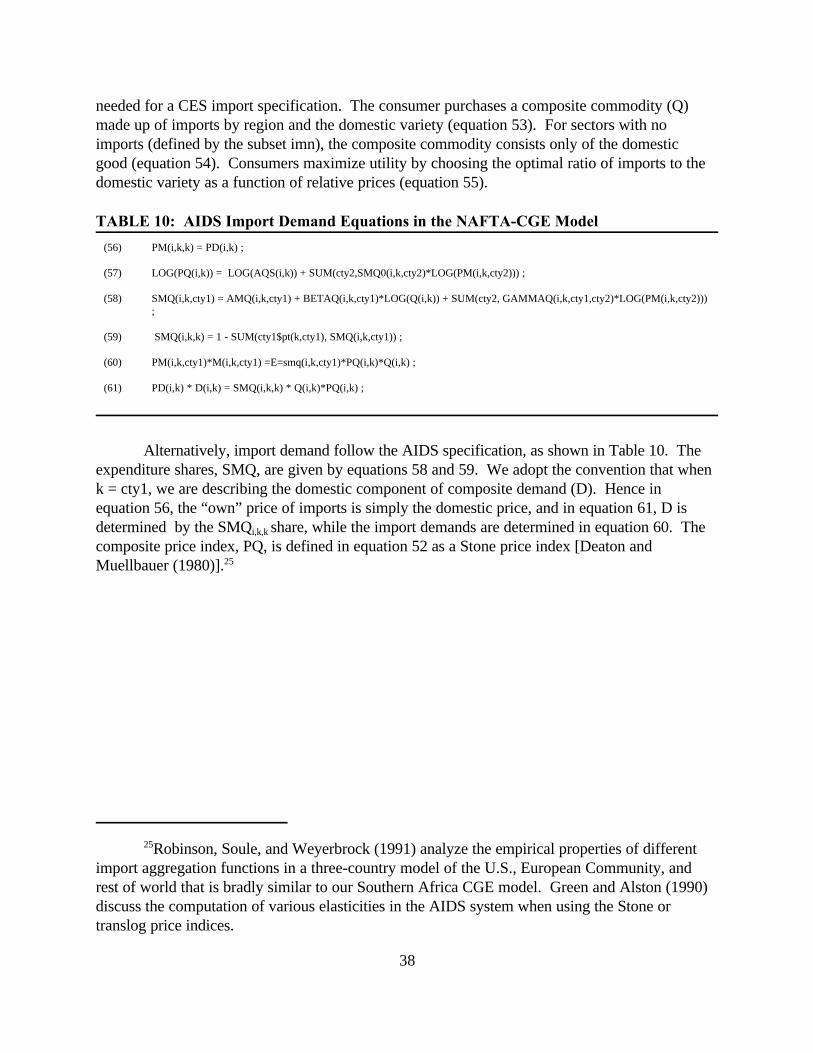
Robinson, Soule, and Weyerbrock (1991) analyze the empirical properties of different25
import aggregation functions in a three-country model of the U.S., European Community, andrest of world that is bradly similar to our Southern Africa CGE model. Green and Alston (1990)discuss the computation of various elasticities in the AIDS system when using the Stone ortranslog price indices.
38
(56) PM(i,k,k) = PD(i,k) ;
(57) LOG(PQ(i,k)) = LOG(AQS(i,k)) + SUM(cty2,SMQ0(i,k,cty2)*LOG(PM(i,k,cty2))) ; (58) SMQ(i,k,cty1) = AMQ(i,k,cty1) + BETAQ(i,k,cty1)*LOG(Q(i,k)) + SUM(cty2, GAMMAQ(i,k,cty1,cty2)*LOG(PM(i,k,cty2)))
;
(59) SMQ(i,k,k) = 1 - SUM(cty1$pt(k,cty1), SMQ(i,k,cty1)) ;
(60) PM(i,k,cty1)*M(i,k,cty1) =E=smq(i,k,cty1)*PQ(i,k)*Q(i,k) ; (61) PD(i,k) * D(i,k) = SMQ(i,k,k) * Q(i,k)*PQ(i,k) ;
TABLE 10: AIDS Import Demand Equations in the NAFTA-CGE Model
needed for a CES import specification. The consumer purchases a composite commodity (Q)made up of imports by region and the domestic variety (equation 53). For sectors with noimports (defined by the subset imn), the composite commodity consists only of the domesticgood (equation 54). Consumers maximize utility by choosing the optimal ratio of imports to thedomestic variety as a function of relative prices (equation 55).
Alternatively, import demand follow the AIDS specification, as shown in Table 10. Theexpenditure shares, SMQ, are given by equations 58 and 59. We adopt the convention that whenk = cty1, we are describing the domestic component of composite demand (D). Hence inequation 56, the “own” price of imports is simply the domestic price, and in equation 61, D isdetermined by the SMQ share, while the import demands are determined in equation 60. Thei,k,k
composite price index, PQ, is defined in equation 52 as a Stone price index [Deaton andMuellbauer (1980)].25
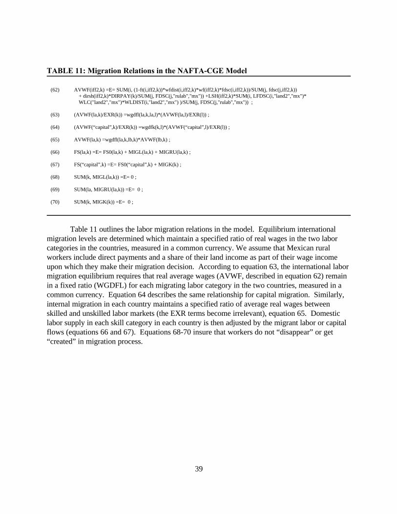
39
(62) AVWF(iff2,k) =E= SUM(i, (1-ft(i,iff2,k))*wfdist(i,iff2,k)*wf(iff2,k)*fdsc(i,iff2,k))/SUM(j, fdsc(j,iff2,k)) + dirsh(iff2,k)*DIRPAY(k)/SUM(j, FDSC(j,"rulab","mx")) +LSH(iff2,k)*SUM(i, LFDSC(i,"land2","mx")* WLC("land2","mx")*WLDIST(i,"land2","mx") )/SUM(j, FDSC(j,"rulab","mx")) ;
(63) (AVWF(la,k)/EXR(k)) =wgdfl(la,k,la,l)*(AVWF(la,l)/EXR(l)) ; (64) (AVWF(“capital”,k)/EXR(k)) =wgdfk(k,l)*(AVWF(“capital”,l)/EXR(l)) ;
(65) AVWF(la,k) =wgdfl(la,k,lb,k)*AVWF(lb,k) ; (66) FS(la,k) =E= FS0(la,k) + MIGL(la,k) + MIGRU(la,k) ;
(67) FS(“capital”,k) =E= FS0(“capital”,k) + MIGK(k) ;
(68) SUM(k, MIGL(la,k)) =E= 0 ;
(69) SUM(la, MIGRU(la,k)) =E= 0 ;
(70) SUM(k, MIGK(k)) =E= 0 ;
TABLE 11: Migration Relations in the NAFTA-CGE Model
Table 11 outlines the labor migration relations in the model. Equilibrium internationalmigration levels are determined which maintain a specified ratio of real wages in the two laborcategories in the countries, measured in a common currency. We assume that Mexican ruralworkers include direct payments and a share of their land income as part of their wage incomeupon which they make their migration decision. According to equation 63, the international labormigration equilibrium requires that real average wages (AVWF, described in equation 62) remainin a fixed ratio (WGDFL) for each migrating labor category in the two countries, measured in acommon currency. Equation 64 describes the same relationship for capital migration. Similarly,internal migration in each country maintains a specified ratio of average real wages betweenskilled and unskilled labor markets (the EXR terms become irrelevant), equation 65. Domesticlabor supply in each skill category in each country is then adjusted by the migrant labor or capitalflows (equations 66 and 67). Equations 68-70 insure that workers do not “disappear” or get“created” in migration process.
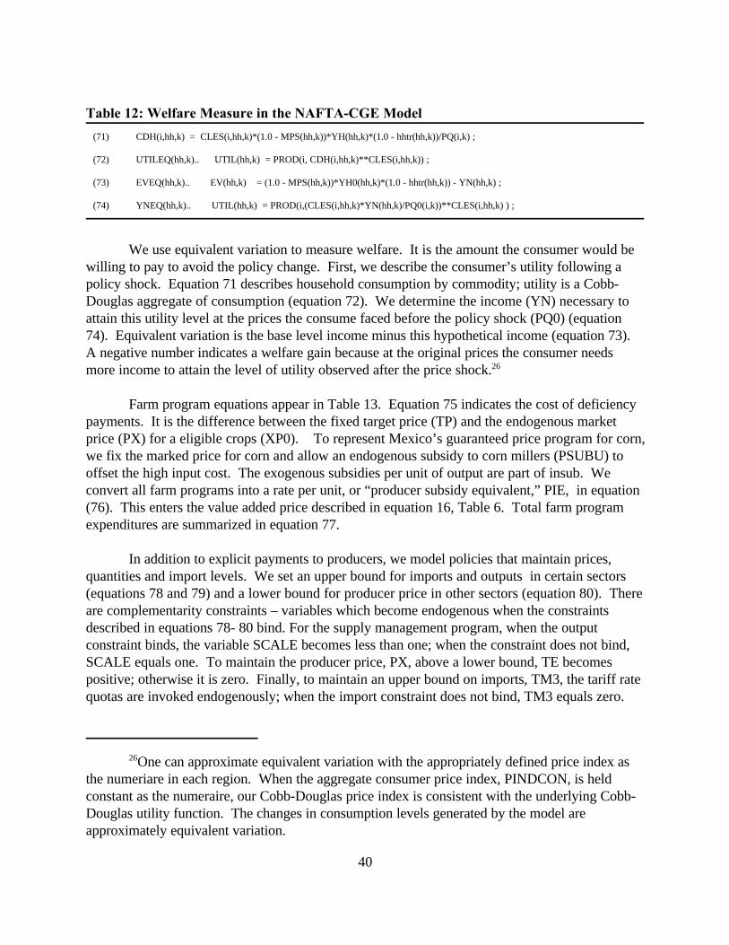
One can approximate equivalent variation with the appropriately defined price index as26
the numeriare in each region. When the aggregate consumer price index, PINDCON, is heldconstant as the numeraire, our Cobb-Douglas price index is consistent with the underlying Cobb-Douglas utility function. The changes in consumption levels generated by the model areapproximately equivalent variation.
40
(71) CDH(i,hh,k) = CLES(i,hh,k)*(1.0 - MPS(hh,k))*YH(hh,k)*(1.0 - hhtr(hh,k))/PQ(i,k) ; (72) UTILEQ(hh,k).. UTIL(hh,k) = PROD(i, CDH(i,hh,k)**CLES(i,hh,k)) ;
(73) EVEQ(hh,k).. EV(hh,k) = (1.0 - MPS(hh,k))*YH0(hh,k)*(1.0 - hhtr(hh,k)) - YN(hh,k) ; (74) YNEQ(hh,k).. UTIL(hh,k) = PROD(i,(CLES(i,hh,k)*YN(hh,k)/PQ0(i,k))**CLES(i,hh,k) ) ;
Table 12: Welfare Measure in the NAFTA-CGE Model
We use equivalent variation to measure welfare. It is the amount the consumer would bewilling to pay to avoid the policy change. First, we describe the consumer’s utility following apolicy shock. Equation 71 describes household consumption by commodity; utility is a Cobb-Douglas aggregate of consumption (equation 72). We determine the income (YN) necessary toattain this utility level at the prices the consume faced before the policy shock (PQ0) (equation74). Equivalent variation is the base level income minus this hypothetical income (equation 73). A negative number indicates a welfare gain because at the original prices the consumer needsmore income to attain the level of utility observed after the price shock.26
Farm program equations appear in Table 13. Equation 75 indicates the cost of deficiencypayments. It is the difference between the fixed target price (TP) and the endogenous marketprice (PX) for a eligible crops (XP0). To represent Mexico’s guaranteed price program for corn,we fix the marked price for corn and allow an endogenous subsidy to corn millers (PSUBU) tooffset the high input cost. The exogenous subsidies per unit of output are part of insub. Weconvert all farm programs into a rate per unit, or “producer subsidy equivalent,” PIE, in equation(76). This enters the value added price described in equation 16, Table 6. Total farm programexpenditures are summarized in equation 77.
In addition to explicit payments to producers, we model policies that maintain prices,quantities and import levels. We set an upper bound for imports and outputs in certain sectors(equations 78 and 79) and a lower bound for producer price in other sectors (equation 80). Thereare complementarity constraints – variables which become endogenous when the constraintsdescribed in equations 78- 80 bind. For the supply management program, when the outputconstraint binds, the variable SCALE becomes less than one; when the constraint does not bind,SCALE equals one. To maintain the producer price, PX, above a lower bound, TE becomespositive; otherwise it is zero. Finally, to maintain an upper bound on imports, TM3, the tariff ratequotas are invoked endogenously; when the import constraint does not bind, TM3 equals zero.

Alternatively, one could fix investment and government consumption shares in GDP27
exogenously.
41
(81) Q(i,k) = INT(i,k)+CDD(i,k)+GD(i,k)+ID(i,k)+DST(i,k);
(82) FS(iff2,k) = SUM(i, FDSC(i,iff2,k)) ;
(83) FSAG(k) = SUM(iag, FDSC(iag,“capital”,k)) ;
(84) FSL(l,k) = SUM(i, LFDSC(i,l,k)) ;
(85) FSAV(k,cty1) = SUM(i, PWM(i,k,cty1)*M(i,k,cty1)) = SUM(i, PWE(i,k,cty1)*E(i,k,cty1)) ; (86) FBAL(k) = SUM(cty1, FSAV(k,cty1)) ;
Table 14: Market-Clearing Equations in the NAFTA-CGE Model
To complete the model, there are a number of additional, “market-clearing” or equilibriumconditions that must be satisfied, as shown in Table 14. Equation 81 is the material balanceequation for each sector, requiring that total composite supply (Q) equal the sum of compositedemands. Equations 82 - 84 provides equilibrium in each factor market. Equation 85 is thebalance condition in the foreign exchange market, requiring that import expenditures equal thesum of export earnings and net foreign capital inflows; equation 86 is the overall trade balanceequation, summing up the bilateral trade balances.
Model Closure
The NAFTA-CGE model permits a number of different “closure”choices that affect themacroeconomic relationships in the model. In all simulations reported in this paper, we haveassumed that the aggregate trade balance (FBAL) is constant for each country, and that theexchange rate (EXR) varies to achieve external balance. Total government spending (GDTOT)and fixed investment (ZFIX) are fixed exogenously. In the government budget constraint,27
equation 34, savings (GOVSAV) and farm program expenditures (FPE) are endogenous, while household transfers (HHT) and enterprise transfers are exogenous. Since investment is fixed,some component of aggregate savings must be free to move; we require that the enterprisesavings rate (ESR) adjust to achieve savings-investment balance. We allow rural-urbanmigration in Mexico, with the factor supply adjusting to maintain average wage differentials.These average wage differentials include payment a share of land return and a share of incomefrom direct payments (see equation 62). All other factors are held in fixed supply and the wageto adjusts.