small area estimation of unemployment: from feasibility to
TRANSCRIPT

Small Area Estimation of Unemployment: From feasibility to implementation
Paper presented at the New Zealand Association of Economists Conference, Wellington, New Zealand,
30 June 2011
Soon Song
Statistical Analyst, Statistical Methods, Statistics New Zealand P O Box 2922
Wellington, New Zealand [email protected]
www.stats.govt.nz

Small Area Estimation of Unemployment: From feasibility to implementation, by Soon Song
2
Crown copyright ©
This work is licensed under the Creative Commons Attribution 3.0 New Zealand licence. You are free
to copy, distribute, and adapt the work for non-commercial purposes, as long as you attribute the work
to Statistics NZ and abide by the other licence terms. Please note you may not use any departmental
or governmental emblem, logo, or coat of arms in any way that infringes any provision of the Flags,
Emblems, and Names Protection Act 1981. Use the wording 'Statistics New Zealand' in your
attribution, not the Statistics NZ logo.
Liability
The opinions, findings, recommendations, and conclusions expressed in this paper are those of the
authors. They do not represent those of Statistics New Zealand, which takes no responsibility for any
omissions or errors in the information in this paper.
Citation
Song, Soon (2011, June). Small area estimation of unemployment: From feasibility to implementation.
Paper presented at the New Zealand Association of Economists Conference, Wellington, New
Zealand.
Small Area Estimation of Unemployment: From feasibility to implementation, by Soon Song
1
Summary
Statistics New Zealand is exploring model-based approaches to produce unemployment
rates at the territorial authority (TA) level, in response to the demand for small area statistics
to support planning, decision making, and service delivery at a local area level. The
Household Labour Force Survey (HLFS) is the main source of national and regional level
information on the labour market. Statistics NZ does not publish unemployment-related
statistics at territorial authority (TA) level using survey direct estimates due to the insufficient
sample size at the TA level.
Statistics NZ has undertaken various research projects to produce TA-level unemployment
rate using HLFS sample data since 2003. In 2009, we investigated the usability of a model
developed for a research programme funded by Eurostat called Enhancing Small Area
Estimation Techniques to meet European Needs (EURAREA). Our investigation was
positive towards producing unemployment rates using HLFS sample data. In 2010, we
proposed to produce an experimental series for TA-level model-based quarterly
unemployment rates, using HLFS sample data and empirical best linear unbiased prediction
(EBLUP) models in EURAREA.
Currently, we use quarterly population estimates at national level for the HLFS benchmarks.
These benchmarks are incorporated into the weighting process system. We do not have
quarterly population estimates at TA level to use as a TA-level benchmark. In this paper, we
propose to produce the TA-level quarterly population estimates. This is a ratio method,
which combines two sources of population estimates, TA-level yearly population estimates
and national-level quarterly population estimates. Firstly, we can calculate the TA-level
proportions of sex by age groups against the national-level total of sex by age groups.
Secondly, we can multiply these proportions to the national-level quarterly population
estimates to produce the TA-level quarterly population estimates.
With these TA-level quarterly population estimates, we propose three options for producing
TA-level weights. These options are:
using the final original weight without alteration
by direct post stratification
by adjusting the final weight.
We decided to use the option of adjusting the final weight. As a result of the TA-level
quarterly population estimates and the adjusted final weight, we could produce estimates of
count and rate statistics at TA level for unemployment, employment, and not in the labour
force.
We tested all models in EURAREA in 2009 project and recommended using the EBLUP
models with covariates of sex, age, and benefit recipients. Based on the recommendation,
we also tested EBLUP models with the proposed covariates as well as ethnicity. In order to
identify a best model, we conducted the following steps.
Firstly, we identified significant covariates for two target variables independently,
unemployment and employment. We used the SAS proc mixed procedure to identify the
Small Area Estimation of Unemployment: From feasibility to implementation, by Soon Song
2
significant individual variables, which are sex, age, ethnicity, and benefit recipients for model
covariates as EURAREA lacks this particular functionality. Secondly, we produced mean
square errors (MSE) for unemployment proportions using several combinations of covariates,
which were the model fit indicators for EBLUPA and EBLUPB. The combinations of
covariates were „sex and age‟, „sex, age and ethnicity‟, and „sex, age, ethnicity, and benefit
recipients‟. We found that EBLUPA produced smaller MSE than EBLUPB, which used all
covariates. Note that we did not attempt using interaction terms of covariates due to the
complexity of organising model input datasets.
Thirdly, based on the four significant covariates, we produced model-based estimates for
EBLUPA (EBLUP unit model) and EBLUPB (EBLUP area model). Also, we produced two
direct estimates using the final weight and the adjusted weight at TA level. We investigated
the four estimates with a time series graph for each sampled TA. Note that we selected eight
sampled TAs based on sample sizes of TAs for the purpose of presentation. The findings
from the comparison of four estimates were:
the direct estimates from the small sizes of the sampled primary sampling units
(PSUs) TAs showed a greater fluctuation over time than the model-based estimates
the estimates of EBLUPA model were slightly higher than those of EBLUPB model
direct estimates using the final weight were not much different from those using the
adjusted final weight
as sample size increased, the gap between the model-based estimates and the
direct estimates was smaller.
Fourthly, we tested the EBLUP time series model and discovered much greater model errors
than EBLUPA and EBLUPB models. Twelve quarters of test data may be insufficient to test
a robust time series analysis. Therefore, we did not carry out further investigation of the
EBLUP time series model.
Lastly, we produced two estimates: the direct estimates at regional level using the original
final weight, and the estimates with summation of the TA-level model-based estimates for
EBLUPA and EBLUPB separately. We compared EBLUPA estimates and EBLUPB
estimates to the regional-level direct estimates separately to check if they were similar. We
checked the following:
time series of estimates for EBLUPA, EBLUPB, and direct estimate
bias of estimates for EBLUPA and EBLUPB, based on the assumption that the
regional-level direct estimates were unbiased
coverage diagnostics for two model-based estimates against direct estimates.
We found that EBLUPB estimates were closer to the direct estimates than EBLUPA
estimates.
So far, we introduced several methods to identify a suitable model: identification of
significant covariates, comparison of MSE for various combinations of covariates and
EBLUP time series model, and comparisons of regional level estimates. However, we were
not able to decide on one conclusive model. In the end, we reached a practical conclusion of
using average estimates of EBLUPA and EBLUPB as our final model.
Small Area Estimation of Unemployment: From feasibility to implementation, by Soon Song
3
1. Introduction
Small area estimation (SAE) is a methodology for producing estimates for a more detailed
level of geography than estimates using direct survey estimation. Sometimes, we use small
area estimation with small domain estimation. However, the two terms are not significantly
different from applying methods. Small domain estimation is logically similar to small area
estimation, which is disaggregated to a finer-level classification. For example, we produce
detailed level industry statistics for business surveys and cross tabulation using detailed
categorical variables.
Statistics NZ acknowledges the demand for small area statistics to support planning,
decision making, and service delivery at a local area level. The HLFS is the main source of
national and regional level information on the labour market. However, it is not able to give
accurate direct estimates of unemployment statistics for every TA in New Zealand due to the
insufficient sample size of some TAs. This research project aims to produce TA-level model-
based quarterly unemployment rates using HLFS survey data with experimental series.
This report covers:
1. Introduction
2. TA level quarterly population
3. Covariate for input model
4. Test data preparation
5. HLFS sample structure
6. Weight issues
7. Overview of testing methods
8. Significant covariates
9. Output comparisons
10. Model decision
11. User validation
12. Discussions
1.1 Definition of terms, abbreviations, and acronyms
Here is a list of terms, abbreviations, and acronyms used in this paper.
SAE: small area estimation
EBLUP: empirical best linear unbiased predictor
EBLUPA: unit level EBLUP model
EBLUPB: area level EBLUP model
EURAREA: enhancing small area estimation techniques to meet European needs,
developed for a research programme funded by Eurostats
Covariate: independent variable in model
ONS: Office for National Statistics of United Kingdom
ILO: International Labour Organization
MSD: Ministry of Social Development
Y variable: dependent variable of interest which is a reference of unemployment or
employment proportion in the working-age population.

Small Area Estimation of Unemployment: From feasibility to implementation, by Soon Song
4
X variable (covariate): independent variable in model; sex, age group, ethnicity, and
MSD benefit recipient.
Direct (survey) estimate: estimate using sample survey weight; this is the standard
estimate method in the current HLFS sample survey
TA-level quarterly population estimate: quarterly population estimate at TA level
produced by two combined sources (TA-level yearly population estimate and
national-level quarterly population estimate produced by Statistics NZ).
1.2 Small areas in New Zealand
Statistics NZ uses these geographic area codes:
Meshblock: the smallest geographic unit for which statistical data is collected.
Meshblocks vary in size, from part of a city block to large areas of rural land.
Meshblocks aggregate to build a larger geographic area, such as an area unit,
territorial authority, and regional council area. In 2011, there are 46,627 meshblocks
in New Zealand.
Area unit: aggregation of meshblocks. An area unit within an urban area normally
has a population of 3,000–5,000,although this can vary, for example, for industrial
areas, port areas, or rural areas within the urban area boundaries. In 2011, there are
2,013 area units in New Zealand.
Territorial authority: aggregation of meshblocks or area units. In the testing period
data, we have 74 TAs, comprising 15 cities and 59 districts. Under the Local
Government Act, there are 67 TAs in 2011.
Regional council area: aggregation of meshblocks and area units. In the testing
period data, we have 16 regions but combined some of them to total 12 regions to
match the HLFS publishing level.
Note that we can define a territorial authority or regional council area as an aggregation of
meshblocks or area units, but cannot define a regional council area as an aggregation of
territorial authorities.
Territorial authority is the small area examined in this report. New Zealand originally
comprised 74 TAs. However, in this report we have merged the Banks Peninsula into the
Christchurch district. Therefore, small areas in this report total 73 TAs including the Chatham
Islands. The distribution of TAs is shown in Table 1-1. The largest TA is Auckland city with a
population of 349,360, while the smallest TA is Chatham Islands with 505.
Table 1-1: Distribution of TAs by population size(1)
Population range Number of TAs %
-< 10,000 16 21.9 10,000 -< 20,000 12 16.4 20,000 -< 50,000 29 39.7
50,000 + 16 21.9 Total 73 100.0
Small Area Estimation of Unemployment: From feasibility to implementation, by Soon Song
5
1. Based on 2006 TA-level yearly population estimate.
1.3 History of SAE projects in SNZ
Statistics NZ has conducted several research projects for SAE since 2001:
expenditure at TA level using the Household Economic Survey
unemployment at TA level using HLFS
business indicators using GST data
assessing disability at district health board level using the Disability Survey.
Recently, two reports about TA-level unemployment estimation were produced, which used
HLFS and MSD data:
Report 1: New approaches to small area estimation of unemployment (Haslett,
Noble, & Zabala, 2008)
Report 2: ‘Small area estimation of unemployment for territorial authorities using
commonly applied estimation models in SAS and R‟ (unpublished report by Ralphs,
Hansen, Song, & Smith, 2010).
Report 1 described models of structure preserving estimation (SPREE), Bayesian, and
relative risk using quarterly HLFS data and auxiliary data from the MSD and the population
census. Report 2 described models in EURAREA packages (described in section 1.4) about
GREG, synthetic, and EBLUP models using artificial yearly HLFS data and auxiliary data
from MSD and the population census.
Report 2 recommended an experimental series for producing unemployment rates for the
quarterly HLFS. This recommendation instigated this current report.
1.4 EURAREA and its application
Statistical agencies and academic researchers have developed different small area
estimation methods to produce detailed statistics using both individual sample data and
aggregated auxiliary data.
Recently, we introduced EURAREA, which was developed by a research programme funded
by Eurostat. The EURAREA development was carried out by a group of national statistics
institutes, universities, and research consultancies from the European Union. The project
was coordinated by the United Kingdom‟s Office for National Statistics (ONS) from January
2001 to June 2004, and was signed off by Eurostat in February 2005.
EURAREA was originally designed to implement a simulation study for small area estimation models containing GREG, synthetic, and EBLUP including direct estimate method. The program modules were developed using intensive SAS macros based on PROC IML. It is very hard for ordinary SAS users to understand the original source macro programs. However, ordinary SAS users can modify parameters in modules to implement once iteration to produce estimates rather than repeated iterations.
In the project, we need three macro modules in EURAREA such as DIRECT (direct survey
estimate method), EBLUPA (unit level EBLUP method), and EBLUPB (area level EBLUP
Small Area Estimation of Unemployment: From feasibility to implementation, by Soon Song
6
method). We organised a user-friendly macro module to implement three models
(%EURArea).
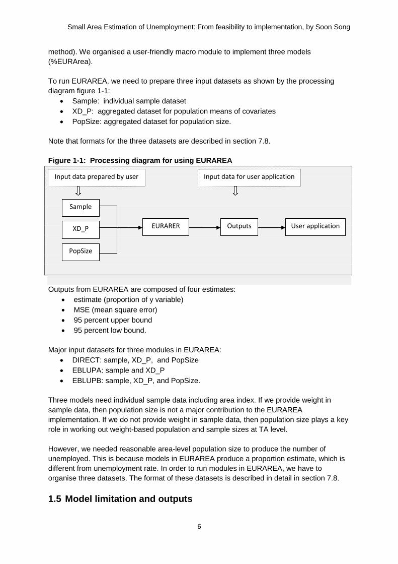
To run EURAREA, we need to prepare three input datasets as shown by the processing
diagram figure 1-1:
Sample: individual sample dataset
XD_P: aggregated dataset for population means of covariates
PopSize: aggregated dataset for population size.
Note that formats for the three datasets are described in section 7.8.
Figure 1-1: Processing diagram for using EURAREA
Outputs from EURAREA are composed of four estimates:
estimate (proportion of y variable)
MSE (mean square error)
95 percent upper bound
95 percent low bound.
Major input datasets for three modules in EURAREA:
DIRECT: sample, XD_P, and PopSize
EBLUPA: sample and XD_P
EBLUPB: sample, XD_P, and PopSize.
Three models need individual sample data including area index. If we provide weight in
sample data, then population size is not a major contribution to the EURAREA
implementation. If we do not provide weight in sample data, then population size plays a key
role in working out weight-based population and sample sizes at TA level.
However, we needed reasonable area-level population size to produce the number of
unemployed. This is because models in EURAREA produce a proportion estimate, which is
different from unemployment rate. In order to run modules in EURAREA, we have to
organise three datasets. The format of these datasets is described in detail in section 7.8.
1.5 Model limitation and outputs
Sample
Outputs EURARER XD_P
PopSize
User application
Input data prepared by user Input data for user application
Small Area Estimation of Unemployment: From feasibility to implementation, by Soon Song
7
1.5.1 Requirement of two models
Each model in EURAREA produces an estimate of y variable with a proportion. If we put
unemployment as the y variable into the processing model, then we can have a proportion
estimate of unemployment in the HLFS population. Strictly speaking, the proportion of
unemployment is different from the unemployment rate.
The International Labour Organization defines unemployment rate as the unemployed
proportion of the labour force population. This population is composed of the unemployed
and employed. However, the HLFS population is composed of three types of persons: the
employed, unemployed, and not in the labour force.
We need two proportion estimates, unemployment and employment, to produce the
unemployment rate. After we produce two proportion estimates, we can derive the proportion
of not in labour force, which is one minus the two proportions of unemployment and
employment.
Therefore, we need to establish at least two models separately instead of three to produce
the unemployment rate. In this report, we established two models to produce the proportion
estimates of unemployment and employment. We processed two models independently
rather than simultaneously because the EURAREA package did not have a multivariate
analysis functionality to handle multi-dependent variables in built-in models.
1.5.2 Derived outputs
If we have the proper population size at TA level, then we can derive some useful variables
based on the proposed estimates in the previous section and the calculation steps in section
7.4. Let us assume that we produce two proportion estimates of unemployment and
employment. We can derive the:
number of unemployed
number of employed
number of not in the labour force
unemployment rate
labour force participation rate.
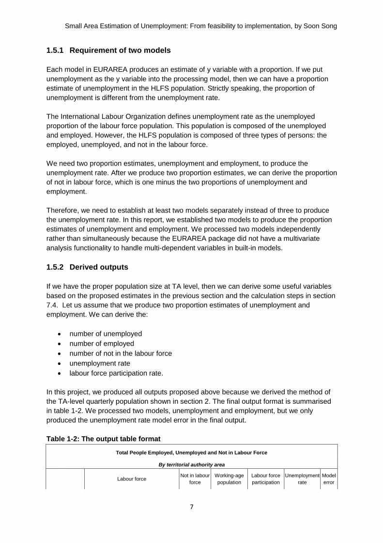
In this project, we produced all outputs proposed above because we derived the method of
the TA-level quarterly population shown in section 2. The final output format is summarised
in table 1-2. We processed two models, unemployment and employment, but we only
produced the unemployment rate model error in the final output.
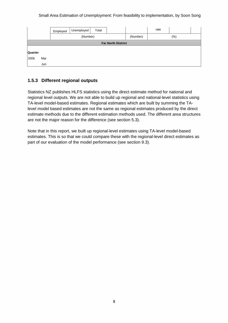
Table 1-2: The output table format
Total People Employed, Unemployed and Not in Labour Force
By territorial authority area
Labour force
Not in labour
force
Working-age
population
Labour force
participation
Unemployment
rate
Model
error
Small Area Estimation of Unemployment: From feasibility to implementation, by Soon Song
8
Employed Unemployed Total rate
(Number) (Number) (%)
Far North District
Quarter
2006
Mar
Jun
1.5.3 Different regional outputs
Statistics NZ publishes HLFS statistics using the direct estimate method for national and
regional level outputs. We are not able to build up regional and national-level statistics using
TA-level model-based estimates. Regional estimates which are built by summing the TA-
level model based estimates are not the same as regional estimates produced by the direct
estimate methods due to the different estimation methods used. The different area structures
are not the major reason for the difference (see section 5.3).
Note that in this report, we built up regional-level estimates using TA-level model-based
estimates. This is so that we could compare these with the regional-level direct estimates as
part of our evaluation of the model performance (see section 9.3).
Small Area Estimation of Unemployment: From feasibility to implementation, by Soon Song
9
2. Territorial authority level quarterly population
The models in EURAREA produce the proportion estimates of target variables, which are
unemployment and employment. In order to produce the number of unemployed and
employed at TA, we need to adopt a proper TA-level quarterly population. We can use this to
produce the TA-level unemployed and employed count estimates and organise the
EURAREA input data of PopSize (population size). Also, we may use it to produce weights
to focus on the TA-level estimates if it is appropriate.
Statistics NZ produces national-level quarterly population estimates to feed into the
current quarterly HLFS weighting system. However, we do not produce TA-level quarterly
population estimates. So, we considered using the following options to obtain TA-level
population: population census, estimation using current HLFS sample, TA-level yearly
population estimate, and estimation of TA-level quarterly population.
2.1 Population census
We can take the TA-level population from population census data. This is the best
population source for the period immediately after the census. However, it does not reflect
the population at the current time.
Furthermore, there is a difference in the definition of population coverage between the
population census and the HLFS survey population. For example, HLFS excludes non-
private dwellings from the survey population whereas the population census includes them.
Population census is not a suitable option for TA-level quarterly HLFS population in terms of
timeliness and the coverage of survey population.
2.2 Estimation using current HLFS sample
We can estimate the TA-level quarterly population from the current period of the HLFS
sample. This is a good option for producing consistent populations of national, regional, and
TA levels.
However, one concern is that we are not able to estimate TA-level populations for all TAs,
because we have three absent TAs in the current HLFS sample (HLFS sample does not
require all TAs to be included). The other concern is that we have to tolerate large sampling
errors for TA-level population estimates, because we have designed the current HLFS
sample to focus on the national-level estimates.
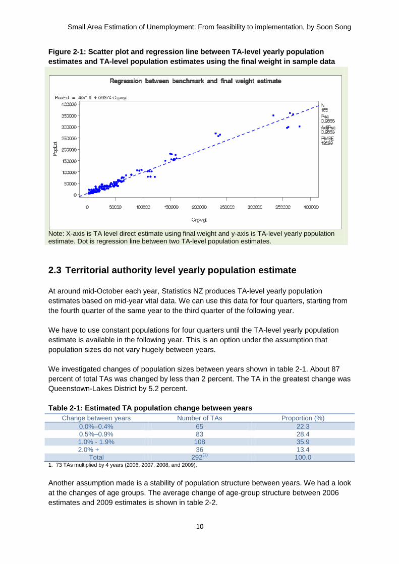
We investigated the relationships between TA-level population estimates calculated from the
HLFS September 2006 quarter sample and the TA-level yearly population estimates
produced in October 2006. Although these two sources were not of the same time point for
exact comparison, they had very close time points. We found very large deviations between
two population estimates for big-sized TAs shown in figure 2-1.
Small Area Estimation of Unemployment: From feasibility to implementation, by Soon Song
10
Figure 2-1: Scatter plot and regression line between TA-level yearly population
estimates and TA-level population estimates using the final weight in sample data
Note: X-axis is TA level direct estimate using final weight and y-axis is TA-level yearly population estimate. Dot is regression line between two TA-level population estimates.
2.3 Territorial authority level yearly population estimate
At around mid-October each year, Statistics NZ produces TA-level yearly population
estimates based on mid-year vital data. We can use this data for four quarters, starting from
the fourth quarter of the same year to the third quarter of the following year.
We have to use constant populations for four quarters until the TA-level yearly population
estimate is available in the following year. This is an option under the assumption that
population sizes do not vary hugely between years.
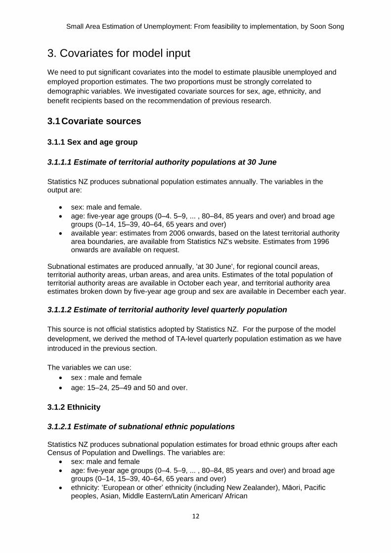
We investigated changes of population sizes between years shown in table 2-1. About 87
percent of total TAs was changed by less than 2 percent. The TA in the greatest change was
Queenstown-Lakes District by 5.2 percent.
Table 2-1: Estimated TA population change between years
Change between years Number of TAs Proportion (%)
0.0%–0.4% 65 22.3 0.5%–0.9% 83 28.4 1.0% - 1.9% 108 35.9
2.0% + 36 13.4 Total 292
(1) 100.0
1. 73 TAs multiplied by 4 years (2006, 2007, 2008, and 2009).
Another assumption made is a stability of population structure between years. We had a look
at the changes of age groups. The average change of age-group structure between 2006
estimates and 2009 estimates is shown in table 2-2.

Small Area Estimation of Unemployment: From feasibility to implementation, by Soon Song
11
Surprisingly, compared with other age groups, the young age group (15–24) was very stable
and the older age group (50 and over) was relatively unstable. However, three age groups
were changed by less than an average of 2 percent every year.
Table 2-2: Average changes of age proportions between 2006 estimates and 2009
estimates
Percent change Age 15-24 (%)
Age 25-49 (%)
Age 50 and over (%)
0.0%–0.4% 95.9 12.3 15.0 0.5%–0.9% 4.1 60.3 83.6 1.0%–2.0% . 27.4 1.4 100.0 100.0 100.0
The TA-level yearly population does not exactly reflect the current TA-level quarterly
populations. However, this is a reasonable option if there are no other options available.
2.4 Estimation of territorial authority level quarterly population
As we investigated the change of age group population structure between years in the
previous section, we found the age group structure of TA to be very stable.
We can apply the idea of the stable distribution of age group to estimate the TA-level
quarterly population estimate. We can estimate it by using two sources: the previous year‟s
TA-level yearly population estimate, and the current quarter‟s national-level population
estimate, which currently uses the HLFS benchmark data for the HLFS weighting process.
Firstly, we calculate the TA-level proportions for sex by age group based on the previous
year‟s TA-level population, that is, jkNationeviousYear
ijkTAeviousYear
ijkTAeviousYear
N
Np
Pr
Pr
Pr , where i=TA, j=sex,
k=age group and N=population. Secondly, we multiply TA-level proportions by the current
quarter‟s national-level population, by sex and age groups, that is:
jkrterNationCurrentQuaijkTAeviousYearijkrterTACurrentQuaNPN *ˆ
Pr .
This method is suitable when we have stable sex by age group structure between years.
2.5 Conclusion of territorial authority level quarterly population
The estimation of TA-level quarterly population using two population sources, described in
section 2.4, would be the best option for reflecting current TA-level populations. In this case,
we have to assume that the population structure is stable between years.
The TA-level quarterly population estimate can be used to calculation of the population
means in the XD_P data and the population sizes of PopSize data. Also, we can use it as
the population benchmark for producing TA-level weight adjustment factor. TA-level
weighting issue will be discussed in the weighting issue (see section 6.2).
Small Area Estimation of Unemployment: From feasibility to implementation, by Soon Song
12
3. Covariates for model input
We need to put significant covariates into the model to estimate plausible unemployed and
employed proportion estimates. The two proportions must be strongly correlated to
demographic variables. We investigated covariate sources for sex, age, ethnicity, and
benefit recipients based on the recommendation of previous research.
3.1 Covariate sources
3.1.1 Sex and age group
3.1.1.1 Estimate of territorial authority populations at 30 June
Statistics NZ produces subnational population estimates annually. The variables in the output are:
sex: male and female.
age: five-year age groups (0–4. 5–9, ... , 80–84, 85 years and over) and broad age groups (0–14, 15–39, 40–64, 65 years and over)
available year: estimates from 2006 onwards, based on the latest territorial authority area boundaries, are available from Statistics NZ's website. Estimates from 1996 onwards are available on request.
Subnational estimates are produced annually, 'at 30 June', for regional council areas, territorial authority areas, urban areas, and area units. Estimates of the total population of territorial authority areas are available in October each year, and territorial authority area estimates broken down by five-year age group and sex are available in December each year.
3.1.1.2 Estimate of territorial authority level quarterly population
This source is not official statistics adopted by Statistics NZ. For the purpose of the model
development, we derived the method of TA-level quarterly population estimation as we have
introduced in the previous section.
The variables we can use:
sex : male and female
age: 15–24, 25–49 and 50 and over.
3.1.2 Ethnicity
3.1.2.1 Estimate of subnational ethnic populations Statistics NZ produces subnational population estimates for broad ethnic groups after each Census of Population and Dwellings. The variables are:
sex: male and female
age: five-year age groups (0–4. 5–9, ... , 80–84, 85 years and over) and broad age groups (0–14, 15–39, 40–64, 65 years and over)
ethnicity: „European or other‟ ethnicity (including New Zealander), Māori, Pacific peoples, Asian, Middle Eastern/Latin American/ African
Small Area Estimation of Unemployment: From feasibility to implementation, by Soon Song
13
available year: 1996, 2001, 2006 The next release of subnational population estimates for broad ethnic groups will occur after the 2013 Census.
3.1.2.2 Population census
We can use ethnicity population from Statistics NZ‟s population census every five years. We
investigated ethnicity distribution change between the 2001 and 2006 Censuses. The
ethnicity composition of the combined Māori and Pacific peoples is stable between two
censuses.
Table 3-1: Change of combined Māori and Pacific peoples between 2001 and 2006
Censuses
Percent change Number of TAs Proportion (%)
0–1 63 86.3
2–3 8 11.0
3+ 2 2.7
Total 73 100.0
3.1.3 Working-age unemployment benefit recipients (aged 18–64)
The Ministry of Social Development produces statistics of unemployment benefit recipients
every quarter. The variables are:
sex: male and female
age: individual age from 18 to 64
ethnicity: European/Pakeha, New Zealand Māori, Chinese/Indian, Pacific peoples
and other
number of benefit recipients
available period: quarter.
3.2 Discussion of covariates
In the preliminary HLFS small area estimation research, we investigated models using
covariates of sex, age group (15–24, 25–49, 50 and over) and MSD benefit recipients. When
the model test was implemented based on artificial HLFS yearly data, we discovered tested
covariates were good for predicting variables for the unemployment rate estimate.
In this project, we are going to estimate quarterly HLFS unemployment-related statistics, so
we may revisit these three variables for unemployment-related statistics prediction. Also, we
can add the ethnicity variable into the covariates to investigate its contribution to accurate
model estimates.
Sex and age group: We can use TA-level yearly population estimates for sex and age
covariates if we do not have any other option. Also, we can use sex and age covariates
estimated by the proposed method of TA-level quarterly population. We can use the same
age group for the quarterly HLFS data as we tested in the previous project. Broad age
category may make sense due to the small sample size of TAs. The wide range of age
Small Area Estimation of Unemployment: From feasibility to implementation, by Soon Song
14
category could reduce errors of TA-level population estimates compared with five-year age
groups. We will stick to a broad age category, which ONS is currently implementing in similar
unemployment model practice.
Ethnicity: In this project, we are going to add the ethnicity covariate into the models based
on the recommendation of the previous project. Ethnicity can be categorised very similarly to
the way we categorise age. We can categorise two ethnic groups (combined one group of
Māori and Pacific peoples and the rest of ethnicities). We will not attempt to test models
using various age and ethnicity groups, as many TA-level population sizes are too small and
there is limited time for testing detailed models.
MSD data: We can use age and ethnicity variables for MSD benefit recipients, but we do not
have enough time to investigate their quality. We will use the number of benefit recipients,
which is aggregated at TA level. We need to investigate age and ethnicity variables in MSD
data to feed into the models.
3.3 Conclusion of covariates for input model
Four covariates will be tested for their significance in the model for predicting unemployment
and employment proportions:
sex and three age groups (15–24, 25–49, 50 and over) will be organised using TA-
level quarterly population estimates produced by part of the HLFS small area
estimation processing system
ethnicity (Māori plus Pacific peoples and others) will be organised using 2006
Population Census ethnicity
MSD data will be used for the number of unemployment benefit recipients at TA level.
Small Area Estimation of Unemployment: From feasibility to implementation, by Soon Song
15
4. Test data preparation
4.1 HLFS data
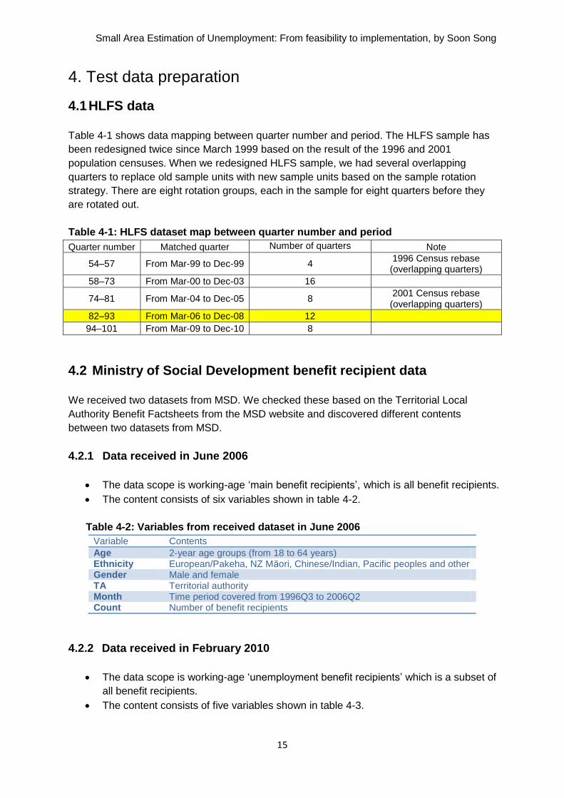
Table 4-1 shows data mapping between quarter number and period. The HLFS sample has
been redesigned twice since March 1999 based on the result of the 1996 and 2001
population censuses. When we redesigned HLFS sample, we had several overlapping
quarters to replace old sample units with new sample units based on the sample rotation
strategy. There are eight rotation groups, each in the sample for eight quarters before they
are rotated out.
Table 4-1: HLFS dataset map between quarter number and period
Quarter number Matched quarter Number of quarters Note
54–57 From Mar-99 to Dec-99 4 1996 Census rebase (overlapping quarters)
58–73 From Mar-00 to Dec-03 16
74–81 From Mar-04 to Dec-05 8 2001 Census rebase (overlapping quarters)
82–93 From Mar-06 to Dec-08 12
94–101 From Mar-09 to Dec-10 8
4.2 Ministry of Social Development benefit recipient data
We received two datasets from MSD. We checked these based on the Territorial Local
Authority Benefit Factsheets from the MSD website and discovered different contents
between two datasets from MSD.
4.2.1 Data received in June 2006
The data scope is working-age „main benefit recipients‟, which is all benefit recipients.
The content consists of six variables shown in table 4-2.
Table 4-2: Variables from received dataset in June 2006
Variable Contents
Age 2-year age groups (from 18 to 64 years) Ethnicity European/Pakeha, NZ Māori, Chinese/Indian, Pacific peoples and other Gender Male and female TA Territorial authority Month Time period covered from 1996Q3 to 2006Q2 Count Number of benefit recipients
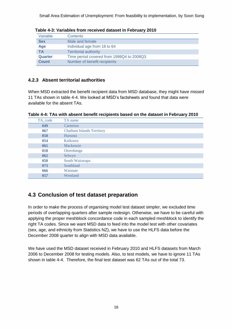
4.2.2 Data received in February 2010
The data scope is working-age „unemployment benefit recipients‟ which is a subset of
all benefit recipients.
The content consists of five variables shown in table 4-3.
Small Area Estimation of Unemployment: From feasibility to implementation, by Soon Song
16
Table 4-3: Variables from received dataset in February 2010
Variable Contents
Sex Male and female
Age Individual age from 18 to 64
TA Territorial authority
Quarter Time period covered from 1998Q4 to 2008Q3
Count Number of benefit recipients
4.2.3 Absent territorial authorities
When MSD extracted the benefit recipient data from MSD database, they might have missed
11 TAs shown in table 4-4. We looked at MSD‟s factsheets and found that data were
available for the absent TAs.
Table 4-4: TAs with absent benefit recipients based on the dataset in February 2010
TA_code TA name
049 Carterton
067 Chatham Islands Territory
058 Hurunui
054 Kaikoura
065 Mackenzie
018 Otorohanga
062 Selwyn
050 South Wairarapa
073 Southland
066 Waimate
057 Westland
4.3 Conclusion of test dataset preparation
In order to make the process of organising model test dataset simpler, we excluded time
periods of overlapping quarters after sample redesign. Otherwise, we have to be careful with
applying the proper meshblock concordance code in each sampled meshblock to identify the
right TA codes. Since we want MSD data to feed into the model test with other covariates
(sex, age, and ethnicity from Statistics NZ), we have to use the HLFS data before the
December 2008 quarter to align with MSD data available.
We have used the MSD dataset received in February 2010 and HLFS datasets from March
2006 to December 2008 for testing models. Also, to test models, we have to ignore 11 TAs
shown in table 4-4. Therefore, the final test dataset was 62 TAs out of the total 73.
Small Area Estimation of Unemployment: From feasibility to implementation, by Soon Song
17
5. HLFS sample
In this section, we discuss an overall HLFS sample structure. If we understand current HLFS
sample structure well, it will be helpful in organising a better model. We had a look at basic
sample features based on data from the March 2006 quarter (quarter number 82 in table 4-
1).
5.1 Sample The sample was designed based on targeting national-level outputs.
We selected about 1800 PSUs, 15,000 households and approximately 30,000 individuals in the civilian non-institutionalised usually resident population aged 15 years and over. The groups that are excluded from the survey sample are: those living in non-private dwellings, long-term residents of old people‟s homes, hospitals and psychiatric institutions; inmates of penal institutions; members of the permanent armed forces; members of the non-New Zealand armed forces; overseas diplomats; overseas visitors who expect to be resident in New Zealand for less than 12 months; those aged under 15 years of age; and people living on offshore islands (except for Waiheke Island). (From „HLFS summary profile‟ in SIM database, Statistics New Zealand internal document.)
5.2 Key outputs
Statistics NZ produces statistics related to the variable of labour force status (unemployment,
employment, and not in labour force) defined by ILO for the working-age population aged 15
years and over. Statistics of the number of employed, unemployed, not in the labour force
and labour force participation rate are produced within 6 weeks of the end of each quarter.
The unemployment rate is one of the major indicators in labour market activity. We produce
it with sex and age group breakdown at the national level and for the 12 regions, which is
calculated based on the direct estimation method.
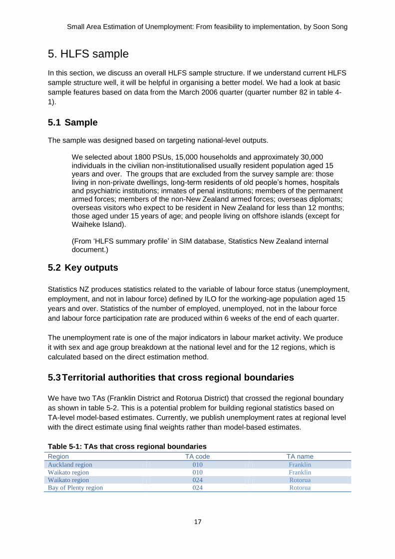
5.3 Territorial authorities that cross regional boundaries
We have two TAs (Franklin District and Rotorua District) that crossed the regional boundary
as shown in table 5-2. This is a potential problem for building regional statistics based on
TA-level model-based estimates. Currently, we publish unemployment rates at regional level
with the direct estimate using final weights rather than model-based estimates.
Table 5-1: TAs that cross regional boundaries
Region TA code TA name
Auckland region 010 Franklin
Waikato region 010 Franklin
Waikato region 024 Rotorua
Bay of Plenty region 024 Rotorua
Small Area Estimation of Unemployment: From feasibility to implementation, by Soon Song
18
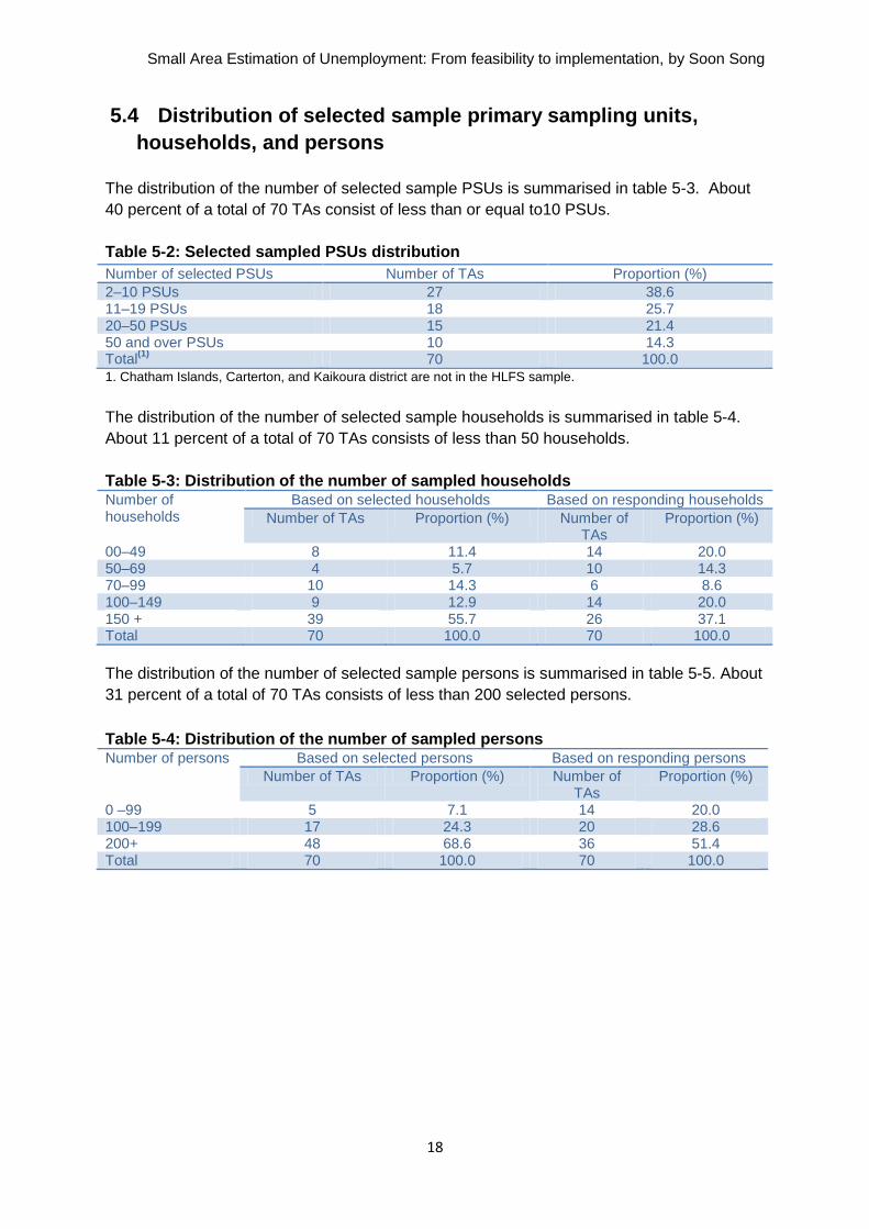
5.4 Distribution of selected sample primary sampling units,
households, and persons
The distribution of the number of selected sample PSUs is summarised in table 5-3. About
40 percent of a total of 70 TAs consist of less than or equal to10 PSUs.
Table 5-2: Selected sampled PSUs distribution
Number of selected PSUs Number of TAs Proportion (%)
2–10 PSUs 27 38.6 11–19 PSUs 18 25.7 20–50 PSUs 15 21.4 50 and over PSUs 10 14.3 Total
(1) 70 100.0
1. Chatham Islands, Carterton, and Kaikoura district are not in the HLFS sample.
The distribution of the number of selected sample households is summarised in table 5-4.
About 11 percent of a total of 70 TAs consists of less than 50 households.
Table 5-3: Distribution of the number of sampled households Number of households
Based on selected households Based on responding households
Number of TAs Proportion (%) Number of TAs
Proportion (%)
00–49 8 11.4 14 20.0 50–69 4 5.7 10 14.3 70–99 10 14.3 6 8.6 100–149 9 12.9 14 20.0 150 + 39 55.7 26 37.1 Total 70 100.0 70 100.0
The distribution of the number of selected sample persons is summarised in table 5-5. About
31 percent of a total of 70 TAs consists of less than 200 selected persons.
Table 5-4: Distribution of the number of sampled persons Number of persons Based on selected persons Based on responding persons
Number of TAs Proportion (%) Number of TAs
Proportion (%)
0 –99 5 7.1 14 20.0 100–199 17 24.3 20 28.6 200+ 48 68.6 36 51.4 Total 70 100.0 70 100.0
Small Area Estimation of Unemployment: From feasibility to implementation, by Soon Song
19
6. Weight issues
We have tested three models (direct, EBLUPA, and EBLUPB) built in the EURAREA
package. Although previous research favoured the EBLUP model, in this project we have
also tested the EBLUPA model to confirm whether the EBLUPB model is better in quarterly
HLFS data. Since the model of direct estimate and EBLUPB requires weight parameter in
module specification in EURAREA, we considered a suitable weight for meeting TA-level
estimates rather than using the final weight produced by current estimation system.
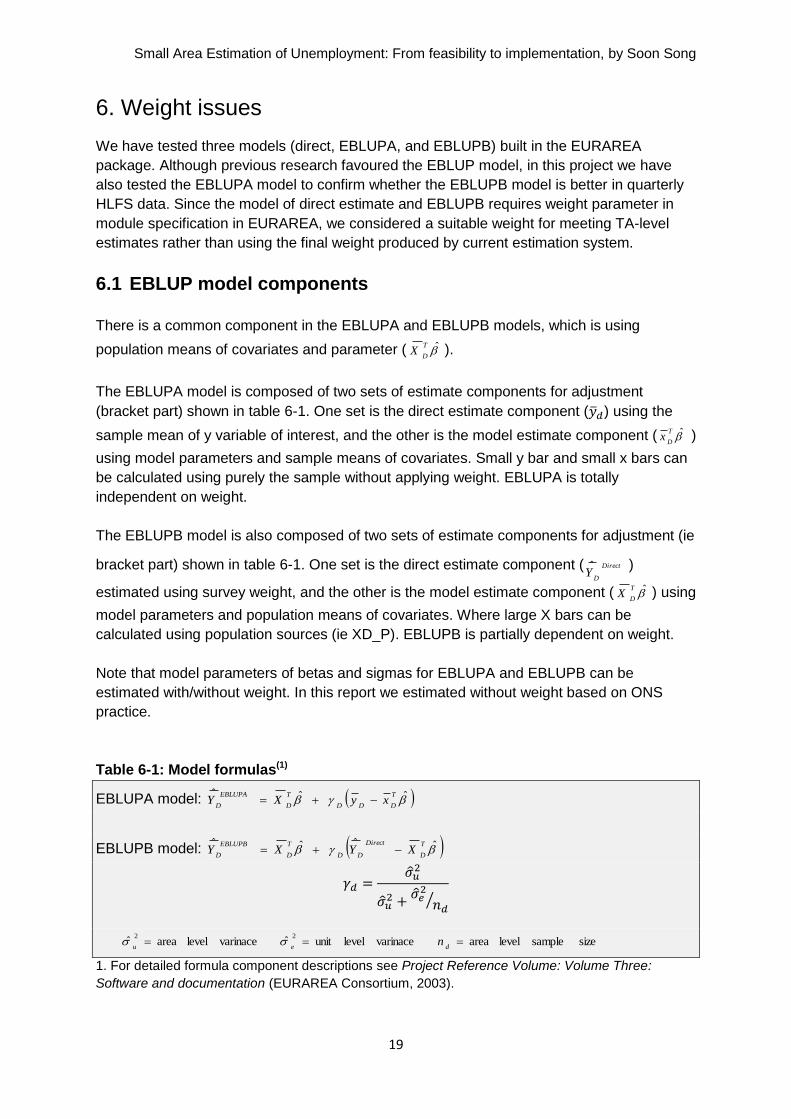
6.1 EBLUP model components
There is a common component in the EBLUPA and EBLUPB models, which is using
population means of covariates and parameter ( T
DX ).
The EBLUPA model is composed of two sets of estimate components for adjustment
(bracket part) shown in table 6-1. One set is the direct estimate component ( ) using the
sample mean of y variable of interest, and the other is the model estimate component ( T
Dx )
using model parameters and sample means of covariates. Small y bar and small x bars can
be calculated using purely the sample without applying weight. EBLUPA is totally
independent on weight.
The EBLUPB model is also composed of two sets of estimate components for adjustment (ie
bracket part) shown in table 6-1. One set is the direct estimate component ( Direct
DYˆ )
estimated using survey weight, and the other is the model estimate component ( T
DX ) using
model parameters and population means of covariates. Where large X bars can be
calculated using population sources (ie XD_P). EBLUPB is partially dependent on weight.
Note that model parameters of betas and sigmas for EBLUPA and EBLUPB can be
estimated with/without weight. In this report we estimated without weight based on ONS
practice.
Table 6-1: Model formulas(1)
EBLUPA model: ˆ ˆˆ T
DDD
T
D
EBLUPA
DxyXY
EBLUPB model: ˆˆ ˆˆ T
D
Direct
DD
T
D
EBLUPB
DXYXY
size sample level area varinacelevelunit ˆ varinacelevel areaˆ22
deu
n
1. For detailed formula component descriptions see Project Reference Volume: Volume Three:
Software and documentation (EURAREA Consortium, 2003).
Small Area Estimation of Unemployment: From feasibility to implementation, by Soon Song
20
6.1.1 Model parameters and variances
Model parameter of betas can be estimated with/without weights. The EURAREA package
can handle modules to estimate parameters in two different ways. One is named ‟standard
module‟, which calculates betas and variances without weights. The other is called ‟weighted
module‟, which calculates betas and variances using weights. Therefore, we needed to
consider whether we could use the final weight or produce another weight for small area
estimation purposes.
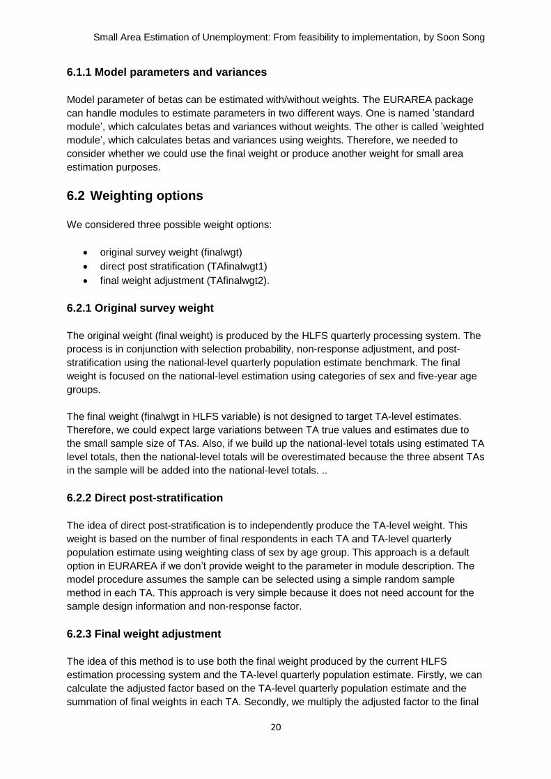
6.2 Weighting options
We considered three possible weight options:
original survey weight (finalwgt)
direct post stratification (TAfinalwgt1)
final weight adjustment (TAfinalwgt2).
6.2.1 Original survey weight
The original weight (final weight) is produced by the HLFS quarterly processing system. The
process is in conjunction with selection probability, non-response adjustment, and post-
stratification using the national-level quarterly population estimate benchmark. The final
weight is focused on the national-level estimation using categories of sex and five-year age
groups.
The final weight (finalwgt in HLFS variable) is not designed to target TA-level estimates.
Therefore, we could expect large variations between TA true values and estimates due to
the small sample size of TAs. Also, if we build up the national-level totals using estimated TA
level totals, then the national-level totals will be overestimated because the three absent TAs
in the sample will be added into the national-level totals. ..
6.2.2 Direct post-stratification
The idea of direct post-stratification is to independently produce the TA-level weight. This
weight is based on the number of final respondents in each TA and TA-level quarterly
population estimate using weighting class of sex by age group. This approach is a default
option in EURAREA if we don‟t provide weight to the parameter in module description. The
model procedure assumes the sample can be selected using a simple random sample
method in each TA. This approach is very simple because it does not need account for the
sample design information and non-response factor.
6.2.3 Final weight adjustment
The idea of this method is to use both the final weight produced by the current HLFS
estimation processing system and the TA-level quarterly population estimate. Firstly, we can
calculate the adjusted factor based on the TA-level quarterly population estimate and the
summation of final weights in each TA. Secondly, we multiply the adjusted factor to the final

Small Area Estimation of Unemployment: From feasibility to implementation, by Soon Song
21
weight in the individual record in sample. This step is to adjust the final weight to reflect only
the population of selected TAs.
6.3 Decision of weight option
Both the final weight and weight of direct post-stratification are not plausible options because
they do not reflect the population of total TAs and sample-design base information. However,
we used all the proposed weights to produce direct estimates in model decision section to
see the difference between estimates.
In the end we decided to use the adjusted weight (TAfinalwgt2) for the final estimates.
Small Area Estimation of Unemployment: From feasibility to implementation, by Soon Song
22
7. Overview of testing methods
This section describes the practical methods applied in model identification using EURAREA.
7.1 EBLUPA and EBLUPB
The previous research indicated that the best model might be the area-level EBLUP model
(ie EBLUPB). That research project was conducted on artificial yearly HLFS data to compare
with the 2001 Census unemployment rate. Since we used quarterly HLFS data in this project,
we tested the unit-level EBLUP model (ie EBLUPA) because underlying quarterly data could
have different characteristics compared with artificial yearly data.
7.2 Direct estimate
We produced direct estimates using weights proposed in the previous weight issue section
in order to appropriately compare these to the model estimates and then check bias under
the assumption of unbiased direct estimate. The direct estimate used as the relative
measurement of efficiency of model-based estimates.
7.3 Significant covariates
Since the EURAREA package was not designed to identify significant covariates for fitting
models, we needed to borrow other tools. In the previous research project, we compared
model parameter estimates between SAS proc mixed and EURAREA. We identified
significant covariates using SAS proc mixed for deciding on model input covariates. In order
to simplify application of covariates into the models, we did not try to apply interaction terms
of covariates for testing the proposed models.
7.4 Outputs and two models
Firstly, we produced two proportions (unemployment and employment) using model-based
estimates and then we produced derived outputs.
Derived outputs using estimates are the:
number of persons employed, unemployed, and not in the labour force
number of persons in the labour force which is the sum of employed and unemployed
number of persons not in the labour force, which is the working-age population minus
the number of persons in the labour force
unemployment rate and labour force participation rate.
We were not able to directly produce the unemployment rate with the proposed models
using the EURAREA. The estimates produced by built-in models in the EURAREA package
are the unemployed and employed proportions of the working-age population, which are
composed of three categories (employed, unemployed, and not in the labour force). The
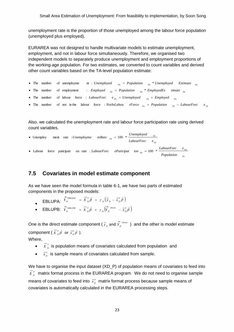
Small Area Estimation of Unemployment: From feasibility to implementation, by Soon Song
23
unemployment rate is the proportion of those unemployed among the labour force population
(unemployed plus employed).
EURAREA was not designed to handle multivariate models to estimate unemployment,
employment, and not in labour force simultaneously. Therefore, we organised two
independent models to separately produce unemployment and employment proportions of
the working-age population. For two estimates, we converted to count variables and derived
other count variables based on the TA-level population estimate:
TATATA
TATATA
TATATA
TATATA
eLabourForcPopulationrForceNotInLabou
EmployedUnemployedeLabourForc
timateEmployedEsPopulationEmployed
EstimateUnemployedPopulationUnemployed
:forcelabour in thenot ofnumber The
:forcelabour ofnumber The
* :employment ofnumber The
* :ntunemployme ofnumber The
Also, we calculated the unemployment rate and labour force participation rate using derived
count variables.
TA
TA
TA
TA
TA
TA
Population
eLabourForcionePaticipatLabourForc
eLabourForc
UnemployedntRateUnemployme
*100 :rateon paticipati forceLabour
*100 :ratement Unemploy
7.5 Covariates in model estimate component
As we have seen the model formula in table 6-1, we have two parts of estimated
components in the proposed models:
EBLUPA: ˆ ˆˆ T
DDD
T
D
EBLUPA
DxyXY
EBLUPB: ˆˆ ˆˆ T
D
Direct
DD
T
D
EBLUPB
DxYXY
One is the direct estimate component (D
y and Direct
DYˆ
) and the other is model estimate
component ( T
DX or
T
Dx ).
Where,
T
DX is population means of covariates calculated from population and
T
Dx is sample means of covariates calculated from sample.
We have to organise the input dataset (XD_P) of population means of covariates to feed into T
DX matrix format process in the EURAREA program. We do not need to organise sample
means of covariates to feed into T
Dx matrix format process because sample means of
covariates is automatically calculated in the EURAREA processing steps.

Small Area Estimation of Unemployment: From feasibility to implementation, by Soon Song
24
In order to organise the input covariate dataset (XD_P), we created indicator variables for all
categorical covariates after ignoring the first category of covariate of interest.
For example, if we want to create the indicator variables of age group composed of three
categories like category of 1 (15–24), category of 2 (25–49) and category of 3 (50 and over),
then we have to create two indicator variables for category of 2 (age2) and category of 3
(age3) and we ignore the first category of 1 (15–24) in the input covariate dataset. Following
these rules, we created XD_P dataset for EURAREA.
The link function for the model estimate component is:
T
DX = β1MSD(proportion) + β2sex2(female proportion) + β3age2(age25-49 proportion) +
β4age3 (age 50 and over proportion) + β5ethnicity(Maori plus Pacific proportion).
7.6 EBLUP time series model
The EURAREA package has a functionality of adapting a time-varying area effect which is
named EBLUP_TS. It is based on a linear mixed model with area level covariates and a
pooled sample estimate within area and time. This assumes that the survey errors are
autocorrelated over time due to the rotating panel nature of the sample. The survey error
autocorrelation structure can be estimated and a model for the survey error can be
developed and combined with a model for the population values.
We tested the EBLUP time series model with the same covariates used for the EBLUPA and
EBLUPB models to determine whether the estimates have been improved (see the results in
section 9.2).
For the detailed EBLUP_TS concept, see Project Reference Volume: Volume Three:
Software and documentation (EURAREA Consortium, 2003).
7.7 Standard version or weighted version for EURAREA
EURAREA has two different versions: the standard version, which does not use weight for
producing coefficients and variances, and the weighted version, which uses weight for
producing coefficients and variances. When ONS developed the EURAREA package, they
discussed the issue of using weight for handling sample survey data.
We compared two model parameters. One was produced using weight option in SAS proc
mixed and the other was produced without weight option in SAS proc mixed. We discovered
different variances between the two outputs. We discussed the two versions with ONS and
followed the ONS practice using the standard version of EURAREA for producing model-
based estimates.
Small Area Estimation of Unemployment: From feasibility to implementation, by Soon Song
25
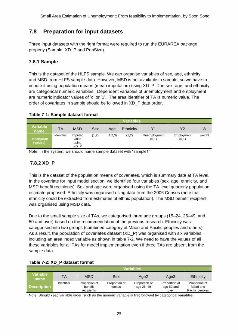
7.8 Preparation for input datasets
Three input datasets with the right format were required to run the EURAREA package
properly (Sample, XD_P and PopSize).
7.8.1 Sample
This is the dataset of the HLFS sample. We can organise variables of sex, age, ethnicity,
and MSD from HLFS sample data. However, MSD is not available in sample, so we have to
impute it using population means (mean imputation) using XD_P. The sex, age, and ethnicity
are categorical numeric variables. Dependent variables of unemployment and employment
are numeric indicator values of ‟o‟ or ‟1‟. The area identifier of TA is numeric value. The
order of covariates in sample should be followed in XD_P data order.
Table 7-1: Sample dataset format
Variables
Variable name
TA MSD Sex Age Ethnicity Y1 Y2 W
Description (values)
Identifier Imputed value using XD_P
(1,2) (1,2,3) (1,2) Unemployment (0,1)
Employment (0,1)
weight
Note: In the system, we should name sample dataset with “sample1”
7.8.2 XD_P
This is the dataset of the population means of covariates, which is summary data at TA level.
In the covariate for input model section, we identified four variables (sex, age, ethnicity, and
MSD benefit recipients). Sex and age were organised using the TA-level quarterly population
estimate proposed. Ethnicity was organised using data from the 2006 Census (note that
ethnicity could be extracted from estimates of ethnic population). The MSD benefit recipient
was organised using MSD data.
Due to the small sample size of TAs, we categorised three age groups (15–24, 25–49, and
50 and over) based on the recommendation of the previous research. Ethnicity was
categorised into two groups (combined category of Māori and Pacific peoples and others).
As a result, the population of covariates dataset (XD_P) was organised with six variables
including an area index variable as shown in table 7-2. We need to have the values of all
these variables for all TAs for model implementation even if three TAs are absent from the
sample data.
Table 7-2: XD_P dataset format
Variables
Variable name
TA MSD Sex Age2 Age3 Ethnicity
Description Identifier Proportion of
benefit recipients
Proportion of female
Proportion of age 25–49
Proportion of age 50 and
over
Proportion of Māori and
Pacific peoples
Note: Should keep variable order, such as the numeric variable is first followed by categorical variables.

Small Area Estimation of Unemployment: From feasibility to implementation, by Soon Song
26
7.8.3 PopSize
This is the dataset of the TA-level population size. We organised the number of persons
using the TA-level quarterly population estimates. We need to have the value for all TAs for
model implementation even if three TAs are absent from the sample data.
Table7-3: PopSize dataset format
Variables
Variable name
TA Popsize
Description Identifier The number of persons
Small Area Estimation of Unemployment: From feasibility to implementation, by Soon Song
27
8. Significant covariates
8.1 Testing significant covariates
We used HLFS 2008 Q4 data to identify significant covariates. We assumed that data from
other periods would have the same pattern as the tested data. Based on the diagnosis
output produced by SAS proc mixed without weight option, we found all covariates were
significant.
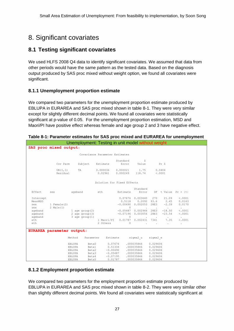
8.1.1 Unemployment proportion estimate
We compared two parameters for the unemployment proportion estimate produced by
EBLUPA in EURAREA and SAS proc mixed shown in table 8-1. They were very similar
except for slightly different decimal points. We found all covariates were statistically
significant at p-value of 0.05. For the unemployment proportion estimation, MSD and
Maori/PI have positive effect whereas female and age group 2 and 3 have negative effect.
Table 8-1: Parameter estimates for SAS proc mixed and EURAREA for unemployment
Unemployment: Testing in unit model without weight SAS proc mixed output:
Covariance Parameter Estimates
Standard Z
Cov Parm Subject Estimate Error Value Pr Z
UN(1,1) TA 0.000036 0.000021 1.75 0.0404
Residual 0.02961 0.000249 118.74 <.0001
Solution for Fixed Effects
Standard
Effect sex ageband eth Estimate Error DF t Value Pr > |t|
Intercept 0.07676 0.003640 270 21.09 <.0001
MeanMSD 0.5118 0.2092 93.6 2.45 0.0163
sex 1 Female(2) -0.00490 0.002053 28E3 -2.39 0.0170
sex 2 Male(1) 0 . . . .
ageband 1 age group(2) -0.05487 0.002966 28E3 -18.50 <.0001
ageband 2 age group(3) -0.07196 0.003056 28E3 -23.54 <.0001
ageband 3 age group(1) 0 . . . .
eth 1 Maori/PI 0.01787 0.002431 7341 7.35 <.0001
eth 2 Others 0 . . . .
EURAREA parameter output:
Method Parameter Estimate sigma2_u sigma2_e
EBLUPA Beta0 0.07676 .000035846 0.029606
EBLUPA Beta1 0.51334 .000035846 0.029606
EBLUPA Beta2 -0.00490 .000035846 0.029606
EBLUPA Beta3 -0.05487 .000035846 0.029606
EBLUPA Beta4 -0.07195 .000035846 0.029606
EBLUPA Beta5 0.01787 .000035846 0.029606
8.1.2 Employment proportion estimate
We compared two parameters for the employment proportion estimate produced by
EBLUPA in EURAREA and SAS proc mixed shown in table 8-2. They were very similar other
than slightly different decimal points. We found all covariates were statistically significant at
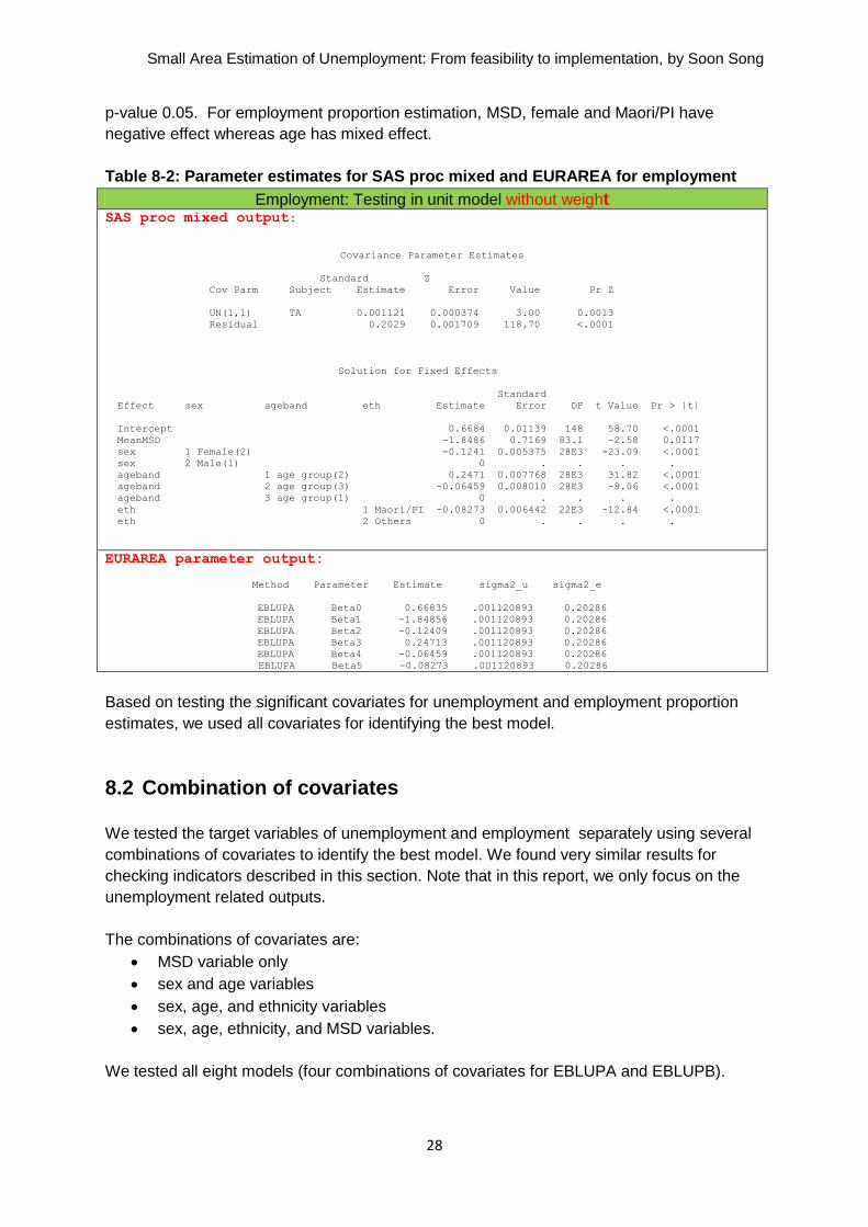
Small Area Estimation of Unemployment: From feasibility to implementation, by Soon Song
28
p-value 0.05. For employment proportion estimation, MSD, female and Maori/PI have
negative effect whereas age has mixed effect.
Table 8-2: Parameter estimates for SAS proc mixed and EURAREA for employment
Employment: Testing in unit model without weight
SAS proc mixed output:
Covariance Parameter Estimates
Standard Z
Cov Parm Subject Estimate Error Value Pr Z
UN(1,1) TA 0.001121 0.000374 3.00 0.0013
Residual 0.2029 0.001709 118.70 <.0001
Solution for Fixed Effects
Standard
Effect sex ageband eth Estimate Error DF t Value Pr > |t|
Intercept 0.6684 0.01139 148 58.70 <.0001
MeanMSD -1.8486 0.7169 83.1 -2.58 0.0117
sex 1 Female(2) -0.1241 0.005375 28E3 -23.09 <.0001
sex 2 Male(1) 0 . . . .
ageband 1 age group(2) 0.2471 0.007768 28E3 31.82 <.0001
ageband 2 age group(3) -0.06459 0.008010 28E3 -8.06 <.0001
ageband 3 age group(1) 0 . . . .
eth 1 Maori/PI -0.08273 0.006442 22E3 -12.84 <.0001
eth 2 Others 0 . . . .
EURAREA parameter output:
Method Parameter Estimate sigma2_u sigma2_e
EBLUPA Beta0 0.66835 .001120893 0.20286
EBLUPA Beta1 -1.84856 .001120893 0.20286
EBLUPA Beta2 -0.12409 .001120893 0.20286
EBLUPA Beta3 0.24713 .001120893 0.20286
EBLUPA Beta4 -0.06459 .001120893 0.20286
EBLUPA Beta5 -0.08273 .001120893 0.20286
Based on testing the significant covariates for unemployment and employment proportion
estimates, we used all covariates for identifying the best model.
8.2 Combination of covariates
We tested the target variables of unemployment and employment separately using several
combinations of covariates to identify the best model. We found very similar results for
checking indicators described in this section. Note that in this report, we only focus on the
unemployment related outputs.
The combinations of covariates are:
MSD variable only
sex and age variables
sex, age, and ethnicity variables
sex, age, ethnicity, and MSD variables.
We tested all eight models (four combinations of covariates for EBLUPA and EBLUPB).
Small Area Estimation of Unemployment: From feasibility to implementation, by Soon Song
29
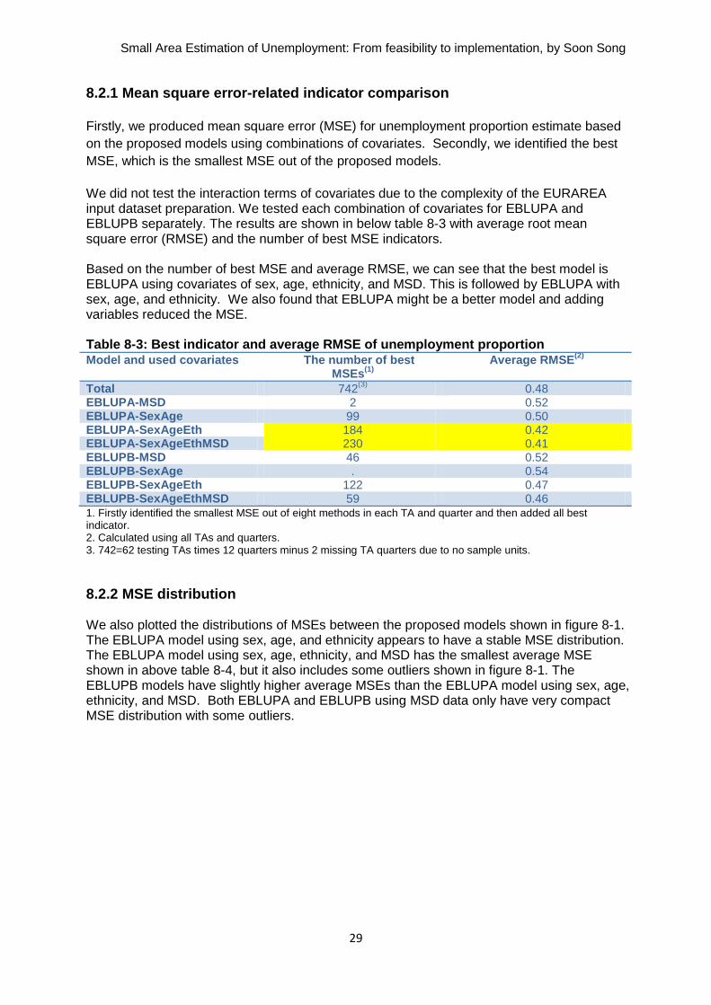
8.2.1 Mean square error-related indicator comparison
Firstly, we produced mean square error (MSE) for unemployment proportion estimate based
on the proposed models using combinations of covariates. Secondly, we identified the best
MSE, which is the smallest MSE out of the proposed models.
We did not test the interaction terms of covariates due to the complexity of the EURAREA input dataset preparation. We tested each combination of covariates for EBLUPA and EBLUPB separately. The results are shown in below table 8-3 with average root mean square error (RMSE) and the number of best MSE indicators. Based on the number of best MSE and average RMSE, we can see that the best model is EBLUPA using covariates of sex, age, ethnicity, and MSD. This is followed by EBLUPA with sex, age, and ethnicity. We also found that EBLUPA might be a better model and adding variables reduced the MSE. Table 8-3: Best indicator and average RMSE of unemployment proportion Model and used covariates The number of best
MSEs(1)
Average RMSE
(2)
Total 742(3)
0.48 EBLUPA-MSD 2 0.52 EBLUPA-SexAge 99 0.50 EBLUPA-SexAgeEth 184 0.42 EBLUPA-SexAgeEthMSD 230 0.41 EBLUPB-MSD 46 0.52 EBLUPB-SexAge . 0.54 EBLUPB-SexAgeEth 122 0.47 EBLUPB-SexAgeEthMSD 59 0.46 1. Firstly identified the smallest MSE out of eight methods in each TA and quarter and then added all best indicator. 2. Calculated using all TAs and quarters. 3. 742=62 testing TAs times 12 quarters minus 2 missing TA quarters due to no sample units.
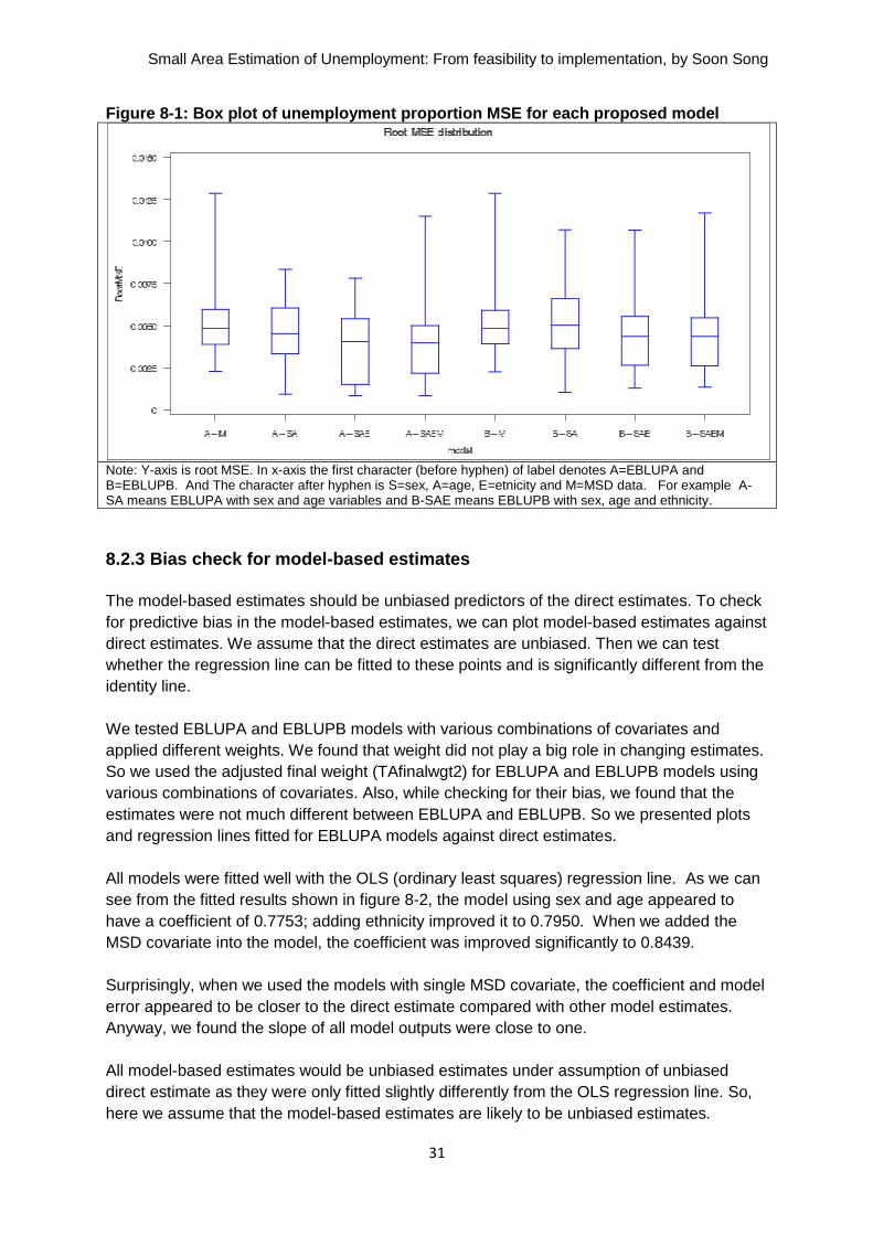
8.2.2 MSE distribution We also plotted the distributions of MSEs between the proposed models shown in figure 8-1. The EBLUPA model using sex, age, and ethnicity appears to have a stable MSE distribution. The EBLUPA model using sex, age, ethnicity, and MSD has the smallest average MSE shown in above table 8-4, but it also includes some outliers shown in figure 8-1. The EBLUPB models have slightly higher average MSEs than the EBLUPA model using sex, age, ethnicity, and MSD. Both EBLUPA and EBLUPB using MSD data only have very compact MSE distribution with some outliers.

Small Area Estimation of Unemployment: From feasibility to implementation, by Soon Song
30
Small Area Estimation of Unemployment: From feasibility to implementation, by Soon Song
31
Figure 8-1: Box plot of unemployment proportion MSE for each proposed model
Note: Y-axis is root MSE. In x-axis the first character (before hyphen) of label denotes A=EBLUPA and B=EBLUPB. And The character after hyphen is S=sex, A=age, E=etnicity and M=MSD data. For example A-SA means EBLUPA with sex and age variables and B-SAE means EBLUPB with sex, age and ethnicity.
8.2.3 Bias check for model-based estimates
The model-based estimates should be unbiased predictors of the direct estimates. To check
for predictive bias in the model-based estimates, we can plot model-based estimates against
direct estimates. We assume that the direct estimates are unbiased. Then we can test
whether the regression line can be fitted to these points and is significantly different from the
identity line.
We tested EBLUPA and EBLUPB models with various combinations of covariates and
applied different weights. We found that weight did not play a big role in changing estimates.
So we used the adjusted final weight (TAfinalwgt2) for EBLUPA and EBLUPB models using
various combinations of covariates. Also, while checking for their bias, we found that the
estimates were not much different between EBLUPA and EBLUPB. So we presented plots
and regression lines fitted for EBLUPA models against direct estimates.
All models were fitted well with the OLS (ordinary least squares) regression line. As we can
see from the fitted results shown in figure 8-2, the model using sex and age appeared to
have a coefficient of 0.7753; adding ethnicity improved it to 0.7950. When we added the
MSD covariate into the model, the coefficient was improved significantly to 0.8439.
Surprisingly, when we used the models with single MSD covariate, the coefficient and model
error appeared to be closer to the direct estimate compared with other model estimates.
Anyway, we found the slope of all model outputs were close to one.
All model-based estimates would be unbiased estimates under assumption of unbiased
direct estimate as they were only fitted slightly differently from the OLS regression line. So,
here we assume that the model-based estimates are likely to be unbiased estimates.

Small Area Estimation of Unemployment: From feasibility to implementation, by Soon Song
32
Figure 8-2: Linearity of EBLUPA model estimate and direct estimate
Using sex and age (β=0.7753 R2=0.78 RMSE=1.98)
Using sex, age and ethnicity (β=0.7950 R2=0.79 RMSE=1.96)
Using sex, age, ethnicity and MSD (β=0.8490 R2=0.81 RMSE=1.88)
Using MSD (β=0.8427 R2=0.82 RMSE=1.76)
Note: Y-axis is unemployment rate(%) using EBLUPB and x-axis is unemployment rate(%) using direct estimate method.
8.3 Discussion of covariate decision
Based on the investigation of average RMSE and best indicator for the proposed eight
models, EBLUPA using sex, age, ethnicity, and MSD covariates appeared to be the best
model, followed by EBLUPA with sex, age, and ethnicity covariates.
Based on the investigation of MSE distribution for the proposed models, EBLUPA with sex,
age, and ethnicity variables looked to be the best model, followed by EBLUPA with sex and
age variables.
Based on MSE comparisons, it was hard for us to tell which model of the combination of
covariates would be the best for the unemployment proportion estimate. EBLUPA using sex,
age, and ethnicity seemed to be a good model. When we added the MSD variable into the
covariates, then the estimate could be slightly improved in terms of the average MSE.

Small Area Estimation of Unemployment: From feasibility to implementation, by Soon Song
33
MSE is only one view of model diagnostics. Hence, we have to look into many different
ways before making a decision on the best model. We decided to use all covariates for
further testing models.
Small Area Estimation of Unemployment: From feasibility to implementation, by Soon Song
34
9. Output comparisons
We produced the model-based estimates of EBLUPA and EBLUPB using sex, age, ethnicity,
and MSD variables. We also produced the direct estimates using the final weight (original
survey weight) and the adjusted final weight. Note that the adjusted final weight has been
discussed in the weighting issue section. The EBLUPB model needs weight parameter for
producing estimates. In order to produce the model-based estimate for EBLUPB, we used
the adjusted final weight (TAfinalwgt2).
We focused on comparing the model-based estimates with the direct estimates, which used
the final weight to determine how much they were different over time. We expected less
variability over time if the model-based estimates performed well. We also compared two
model-based estimates of EBLUPA and EBLUPB to determine how much they were different
over time.
Note that in this section, we will only discuss unemployment rate estimates.
9.1 Comparison of territorial authority level estimates
In order to compare estimates, we made four groups of TAs based on the number of
selected sample PSUs for the 2006 Q1 HLFS (the groups of TAs can be found in the sample
structure section). Both size A and size B are small sizes of sampled PSU TAs, size C is a
medium size of sampled PSU TAs, and size D is a large size of sampled PSU TAs.
For visual illustration, we selected two sample TAs in each size group:
size A (02-10 PSUs): Kawerau district and Wairoa district
size B (11-19 PSUs): Waipa district and Tararua district
size C (20-50 PSUs): Tauranga city and Porirua city
size D (50 over PSUs): New Plymouth district and Auckland city.
Note: Auckland city is not super city.
9.1.1 Size A and size B
We illustrated findings together for size A in figure 9-1 and size B in figure 9-2. All TAs in
size A and size B appeared to have very similar pattern of direct estimates, which had large
variation over time. This must have happened due to the small sample size. Estimates of
EBLUPA were slightly higher than those of EBLUPB in most periods. As we expected it, we
proved that the direct estimates showed greater variation over time than the model-based
estimates. We could see little difference between direct estimate using the final weight and
direct estimate using the adjusted final weight.

Small Area Estimation of Unemployment: From feasibility to implementation, by Soon Song
35
Figure 9-1
Comparison between EBLUP model estimates and direct estimates for size A
Size A(Kawerau) Size A (Wairoa)
Note: Red line=EBLUPA, blue line=EBLUPB, green line= direct estimate using the original final weight and black line=direct estimate using the adjusted final weight. Y-axis is unemployment rate(%) and x-axis is quarter
Figure 9-2
Comparison between EBLUP model estimates and direct estimates for size B
Size B (Waipa) Size B (Tararua)
Note: Red line=EBLUPA, blue line=EBLUPB, green line= direct estimate using the original final weight and black line=direct estimate using the adjusted final weight. Y-axis is unemployment rate(%) and x-axis is quarter
9.1.2 Size C
Small Area Estimation of Unemployment: From feasibility to implementation, by Soon Song
36
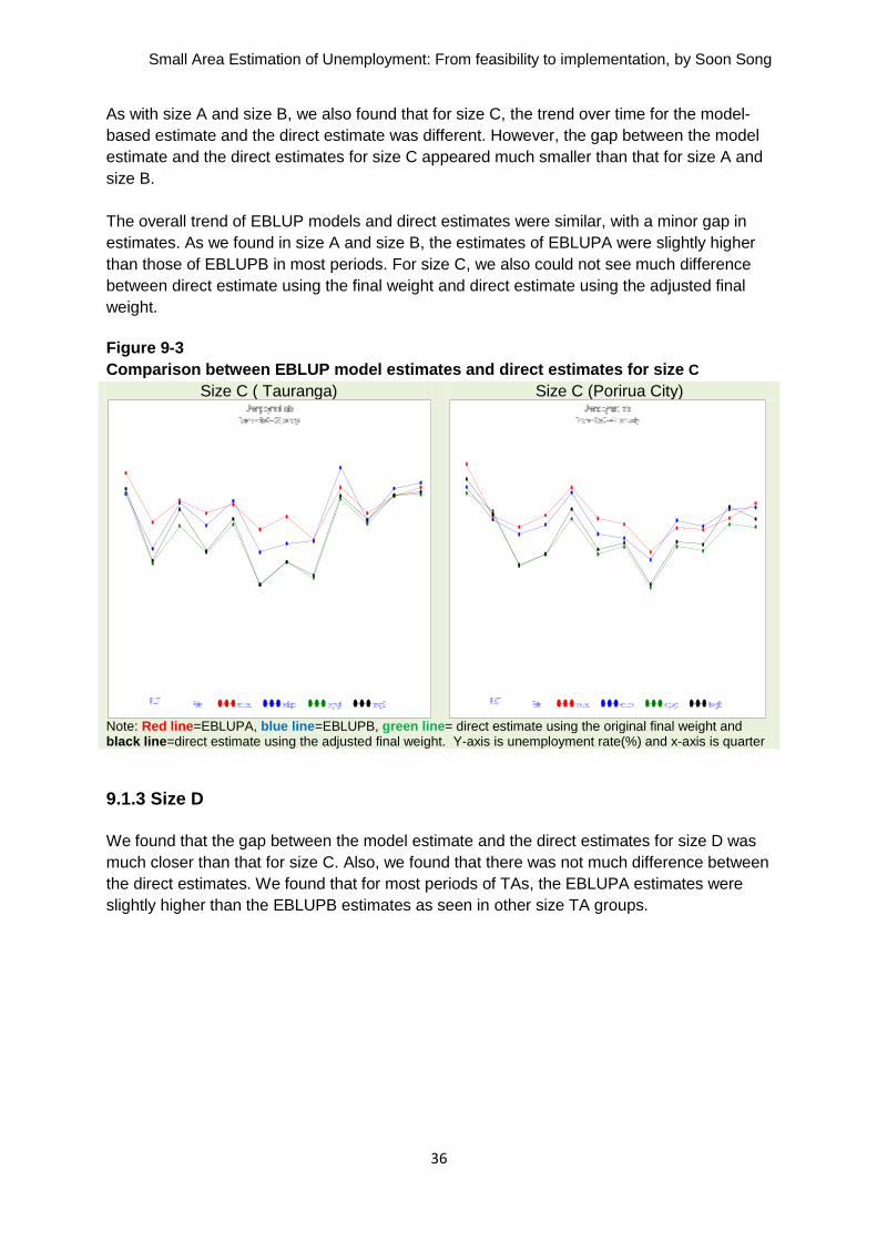
As with size A and size B, we also found that for size C, the trend over time for the model-
based estimate and the direct estimate was different. However, the gap between the model
estimate and the direct estimates for size C appeared much smaller than that for size A and
size B.
The overall trend of EBLUP models and direct estimates were similar, with a minor gap in
estimates. As we found in size A and size B, the estimates of EBLUPA were slightly higher
than those of EBLUPB in most periods. For size C, we also could not see much difference
between direct estimate using the final weight and direct estimate using the adjusted final
weight.
Figure 9-3
Comparison between EBLUP model estimates and direct estimates for size C
Size C ( Tauranga) Size C (Porirua City)
Note: Red line=EBLUPA, blue line=EBLUPB, green line= direct estimate using the original final weight and black line=direct estimate using the adjusted final weight. Y-axis is unemployment rate(%) and x-axis is quarter
9.1.3 Size D
We found that the gap between the model estimate and the direct estimates for size D was
much closer than that for size C. Also, we found that there was not much difference between
the direct estimates. We found that for most periods of TAs, the EBLUPA estimates were
slightly higher than the EBLUPB estimates as seen in other size TA groups.

Small Area Estimation of Unemployment: From feasibility to implementation, by Soon Song
37
Figure 9-4
Comparison between EBLUP model estimates and direct estimates for size D
Size D (New Plymouth) Size D (Auckland City)
Note: Red line=EBLUPA, blue line=EBLUPB, green line= direct estimate using the original final weight and black line=direct estimate using the adjusted final weight. Y-axis is unemployment rate(%) and x-axis is quarter
We quantified the differences between average EBLUP model-based estimates and the
average direct estimates. Note that the average EBLUP model-based estimate was
calculated using EBLUPA and EBLUPB estimates and the average direct estimate was
calculated using the direct estimate based on the final weight and the direct estimate based
on the adjusted final weight. Table 9-1 shows the small size of size A was 2.3 percent and
the large size of size D was 0.5 percent.
Table 9-1: Difference between average EBLUP model-based estimates and average direct
estimates
TA size group Average difference (%)
Size A (02–10 sample PSUs) 2.3 Size B (11–19 sample PSUs) 1.4 Size C (20–50 sample PSUs) 0.9
Size D (50 and over sample PSUs) 0.5
9.1.4 General findings between model-based estimates and direct estimates
We have summarised major findings described in the above group analysis:
The direct estimates from the small sizes of sampled PSU TAs showed a greater
fluctuation over time than the model-based estimates.
The estimates of EBLUPA model were slightly higher than those of EBLUPB model.
Direct estimates using the final weight were not much different from those using the
adjusted final weight.
As sample size increased, the gap between the model-based estimates and the
direct estimates was closer.
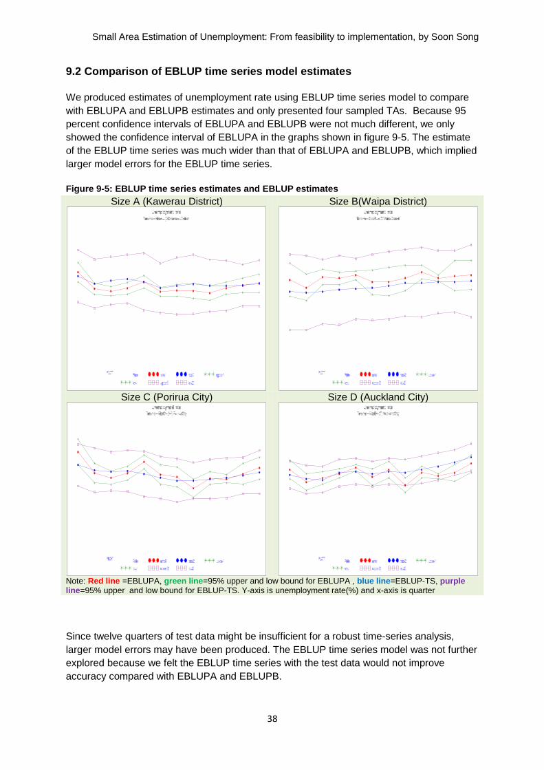
Small Area Estimation of Unemployment: From feasibility to implementation, by Soon Song
38
9.2 Comparison of EBLUP time series model estimates
We produced estimates of unemployment rate using EBLUP time series model to compare
with EBLUPA and EBLUPB estimates and only presented four sampled TAs. Because 95
percent confidence intervals of EBLUPA and EBLUPB were not much different, we only
showed the confidence interval of EBLUPA in the graphs shown in figure 9-5. The estimate
of the EBLUP time series was much wider than that of EBLUPA and EBLUPB, which implied
larger model errors for the EBLUP time series.
Figure 9-5: EBLUP time series estimates and EBLUP estimates
Size A (Kawerau District) Size B(Waipa District)
Size C (Porirua City) Size D (Auckland City)
Note: Red line =EBLUPA, green line=95% upper and low bound for EBLUPA , blue line=EBLUP-TS, purple line=95% upper and low bound for EBLUP-TS. Y-axis is unemployment rate(%) and x-axis is quarter
Since twelve quarters of test data might be insufficient for a robust time-series analysis,
larger model errors may have been produced. The EBLUP time series model was not further
explored because we felt the EBLUP time series with the test data would not improve
accuracy compared with EBLUPA and EBLUPB.
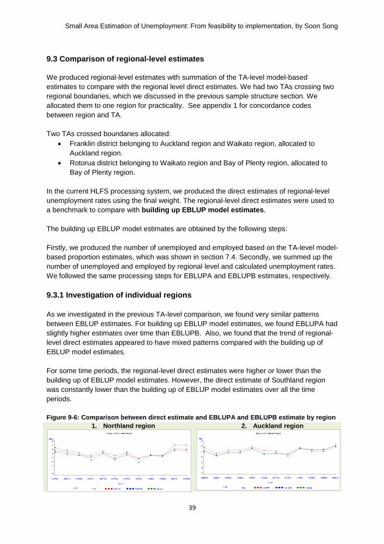
Small Area Estimation of Unemployment: From feasibility to implementation, by Soon Song
39
9.3 Comparison of regional-level estimates
We produced regional-level estimates with summation of the TA-level model-based
estimates to compare with the regional level direct estimates. We had two TAs crossing two
regional boundaries, which we discussed in the previous sample structure section. We
allocated them to one region for practicality. See appendix 1 for concordance codes
between region and TA.
Two TAs crossed boundaries allocated:
Franklin district belonging to Auckland region and Waikato region, allocated to
Auckland region.
Rotorua district belonging to Waikato region and Bay of Plenty region, allocated to
Bay of Plenty region.
In the current HLFS processing system, we produced the direct estimates of regional-level
unemployment rates using the final weight. The regional-level direct estimates were used to
a benchmark to compare with building up EBLUP model estimates.
The building up EBLUP model estimates are obtained by the following steps:
Firstly, we produced the number of unemployed and employed based on the TA-level model-
based proportion estimates, which was shown in section 7.4. Secondly, we summed up the
number of unemployed and employed by regional level and calculated unemployment rates.
We followed the same processing steps for EBLUPA and EBLUPB estimates, respectively.
9.3.1 Investigation of individual regions
As we investigated in the previous TA-level comparison, we found very similar patterns
between EBLUP estimates. For building up EBLUP model estimates, we found EBLUPA had
slightly higher estimates over time than EBLUPB. Also, we found that the trend of regional-
level direct estimates appeared to have mixed patterns compared with the building up of
EBLUP model estimates.
For some time periods, the regional-level direct estimates were higher or lower than the
building up of EBLUP model estimates. However, the direct estimate of Southland region
was constantly lower than the building up of EBLUP model estimates over all the time
periods.
Figure 9-6: Comparison between direct estimate and EBLUPA and EBLUPB estimate by region
1. Northland region 2. Auckland region

Small Area Estimation of Unemployment: From feasibility to implementation, by Soon Song
40
3. Waikato region 4. Bay of Plenty region
5. Gisborne/Hawke’s Bay regions 6. Taranaki region
7. Manawatu-Wanganui region 8. Wellington region
9.West Coast/Tasman/Nelson region 10. Canterbury region
11. Otago region 12. Southland region
Note: Red line=EBLUPA estimate, blue line=EBLUPB and green line= estimate using the original final weight.
Y-axis is unemployment rate(%) and x-axis is quarter
9.3.2 Bias check for the building up of model estimates
We checked whether building up the model estimates were unbiased or not, based on
plotting two estimates. This comparison was conducted under the assumption that the
regional-level direct estimates are unbiased. We compared the regional-level direct
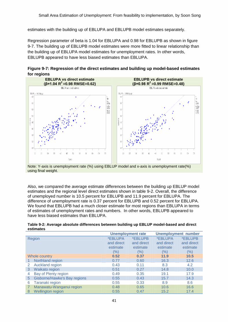
Small Area Estimation of Unemployment: From feasibility to implementation, by Soon Song
41
estimates with the building up of EBLUPA and EBLUPB model estimates separately.
Regression parameter of beta is 1.04 for EBLUPA and 0.98 for EBLUPB as shown in figure
9-7. The building up of EBLUPB model estimates were more fitted to linear relationship than
the building up of EBLUPA model estimates for unemployment rates. In other words,
EBLUPB appeared to have less biased estimates than EBLUPA.
Figure 9-7: Regression of the direct estimates and building up model-based estimates
for regions
EBLUPA vs direct estimate (β=1.04 R
2 =0.98 RMSE=0.62)
EBLUPB vs direct estimate (β=0.98 R
2 =0.99 RMSE=0.48)
Note: Y-axis is unemployment rate (%) using EBLUP model and x-axis is unemployment rate(%) using final weight.
Also, we compared the average estimate differences between the building up EBLUP model estimates and the regional level direct estimates shown in table 9-2. Overall, the difference of unemployed number is 10.5 percent for EBLUPB and 11.9 percent for EBLUPA. The difference of unemployment rate is 0.37 percent for EBLUPB and 0.52 percent for EBLUPA. We found that EBLUPB had a much closer estimate for most regions than EBLUPA in terms of estimates of unemployment rates and numbers. In other words, EBLUPB appeared to have less biased estimates than EBLUPA. Table 9-2: Average absolute differences between building up EBLUP model-based and direct estimates
Unemployment rate Unemployment number
Region *EBLUPA and direct estimate
(%)
*EBLUPB and direct estimate
(%)
*EBLUPA and direct estimate
(%)
*EBLUPB and direct estimate
(%) Whole country 0.52 0.37 11.9 10.5 1 Northland region 0.77 0.60 16.3 12.6 2 Auckland region 0.43 0.11 8.3 4.2 3 Waikato region 0.51 0.27 14.8 10.0 4 Bay of Plenty region 0.49 0.35 19.1 17.9 5 Gisborne/Hawke's Bay regions 0.55 0.43 15.7 14.3 6 Taranaki region 0.55 0.33 8.9 8.6 7 Manawatu-Wanganui region 0.48 0.65 10.6 16.6 8 Wellington region 0.55 0.47 15.2 17.4
Small Area Estimation of Unemployment: From feasibility to implementation, by Soon Song
42
9 West Coast/Tasman/Nelson/Marlborou 0.21 0.25 9.3 14.6 10 Canterbury region 0.33 0.16 7.6 13.9 11 Otago region 0.52 0.28 20.1 9.2 12 Southland region 0.86 0.58 11.9 7.1
Note: EBLUPA and EBLUPB estimates using sex, age, ethnicity, and MSD covariates.
9.4 Investigation of coverage diagnostics
This diagnostic evaluates the validity of the confidence intervals generated by the model-
based estimates. The diagnostic is the measure of overlap between the 95 percent
confidence intervals for the direct estimates and those for the model-based estimates.
We checked whether the 95 percent confidence intervals of the direct estimates contained
EBLUPA and EBLUPB model estimates. As shown in table 9-3, 9.2 percent of EBLUPA and
6.6 percent of EBLUPB estimates were not included into the confidence intervals of the
direct estimates. Conversely, we also checked whether the 95 percent confidence intervals
of the EBLUP estimates contained in the direct estimates. A proportion of 43.9 percent of
EBLUPA and 35.8 percent of EBLUPB were not included into the confidence intervals of
EBLUP model estimates. EBLUPB is likely to be more inclusive than EBLUPA.
Table 9-3: Outside proportions of 95 percent confidence intervals for direct and
EBLUP estimates
Total cases EBLUPA estimates beyond 95% confidence interval of
direct estimate
EBLUPB estimates beyond 95% confidence interval of
direct estimate
742 68 (9.2%) 49 (6.6%)
Direct estimates beyond 95% confidence interval of EBLUPA
estimate
Direct estimates beyond 95% confidence interval of EBLUPB estimate
742 326 (43.9%) 266 (35.8%)
Small Area Estimation of Unemployment: From feasibility to implementation, by Soon Song
43
10. Model decision
We summarise the major findings from the output comparison section and EBLUP model
components:
EBLUPA model is totally free of survey weight, whereas EBLUPB model is partially
dependent on weight. If we choose EBLUPA as our model, then we will lose weight
contribution. HLFS is a sample survey data, so weight should be an important role for
estimation.
Also, as seen in regional level comparison and coverage diagnostic sections about
unemployment rate estimates, EBLUPB was closer to the direct estimates than
EBLUPA.
As seen in the MSE comparison section, EBLUPA had slightly smaller model errors
than EBLUPB.
For most periods of TAs, the EBLUPA estimates were slightly higher than the
EBLUPB estimates. We are not able to prove which one is closer to the true values.
EBLUP time series model was out of our ideal range, because we did not carry out
in-depth investigations and it produced large model errors compared with EBLUP
models.
It was difficult to decide on one conclusive model due to the varied outcomes of all the
comparisons made. In the end, we decided to use an average of EBLUPA and EBLUPB
estimates as our final model using the covariates of sex, age, ethnicity, and MSD benefit
recipient.

Small Area Estimation of Unemployment: From feasibility to implementation, by Soon Song
44
11. User validation
In the previous sections, we discussed the test dataset composed of 62 TAs, which were the
common TAs between HLFS and MSD data from Q1 2006 to Q4 2008. However, we
produced the final experimental estimates from Q1 2006 to Q4 2009 for 73 TAs without
using MSD covariate.
The HLFS team will carry out a user validation exercise for the estimates produced by our
average of the EBLUP models. They will check the estimates against their subject
knowledge and 2006 Census results. We may adjust the final model based on their
comments.
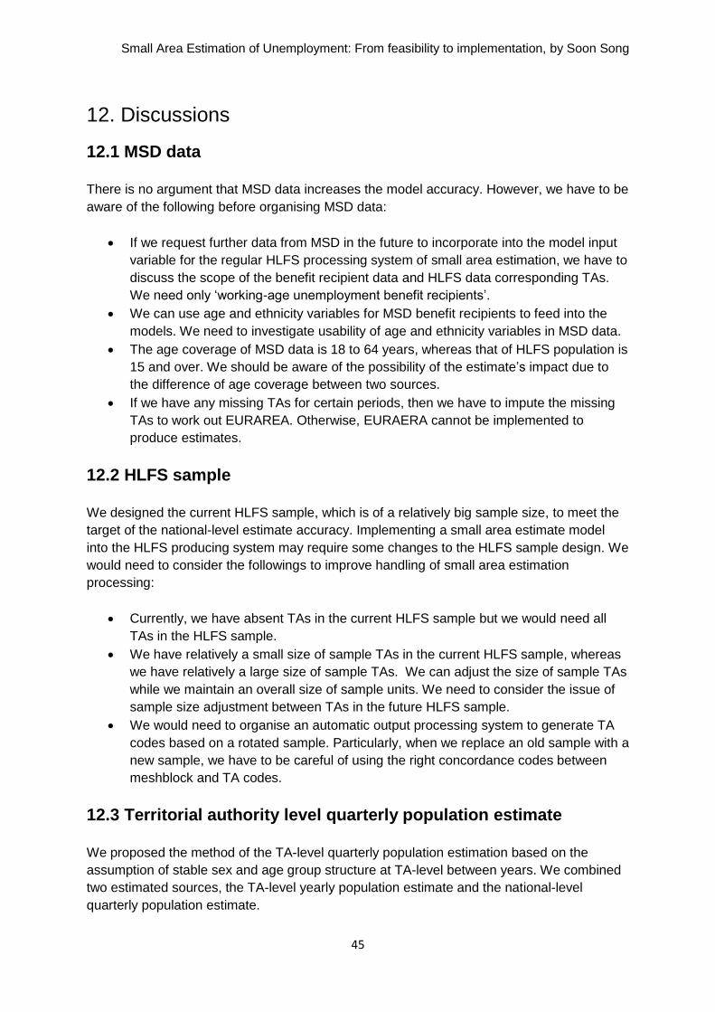
Small Area Estimation of Unemployment: From feasibility to implementation, by Soon Song
45
12. Discussions
12.1 MSD data
There is no argument that MSD data increases the model accuracy. However, we have to be
aware of the following before organising MSD data:
If we request further data from MSD in the future to incorporate into the model input
variable for the regular HLFS processing system of small area estimation, we have to
discuss the scope of the benefit recipient data and HLFS data corresponding TAs.
We need only „working-age unemployment benefit recipients‟.
We can use age and ethnicity variables for MSD benefit recipients to feed into the
models. We need to investigate usability of age and ethnicity variables in MSD data.
The age coverage of MSD data is 18 to 64 years, whereas that of HLFS population is
15 and over. We should be aware of the possibility of the estimate‟s impact due to
the difference of age coverage between two sources.
If we have any missing TAs for certain periods, then we have to impute the missing
TAs to work out EURAREA. Otherwise, EURAERA cannot be implemented to
produce estimates.
12.2 HLFS sample
We designed the current HLFS sample, which is of a relatively big sample size, to meet the
target of the national-level estimate accuracy. Implementing a small area estimate model
into the HLFS producing system may require some changes to the HLFS sample design. We
would need to consider the followings to improve handling of small area estimation
processing:
Currently, we have absent TAs in the current HLFS sample but we would need all
TAs in the HLFS sample.
We have relatively a small size of sample TAs in the current HLFS sample, whereas
we have relatively a large size of sample TAs. We can adjust the size of sample TAs
while we maintain an overall size of sample units. We need to consider the issue of
sample size adjustment between TAs in the future HLFS sample.
We would need to organise an automatic output processing system to generate TA
codes based on a rotated sample. Particularly, when we replace an old sample with a
new sample, we have to be careful of using the right concordance codes between
meshblock and TA codes.
12.3 Territorial authority level quarterly population estimate
We proposed the method of the TA-level quarterly population estimation based on the
assumption of stable sex and age group structure at TA-level between years. We combined
two estimated sources, the TA-level yearly population estimate and the national-level
quarterly population estimate.

Small Area Estimation of Unemployment: From feasibility to implementation, by Soon Song
46
We used this TA-level quarterly population estimate with a population benchmark to revise
the final weight and create the population means of XD_P, which was the model input data.
Therefore, it plays a very important role in the model-based estimates. We would need a
reliable population estimate at TA level to produce accurate estimates for variables of
interest.
12.4 Model improvement and EURAREA
We processed two models of unemployment and employment independently rather than
simultaneously because EURAREA is not capable of multivariate analysis functionality.
Therefore, we cannot measure the interaction impact of unemployment and employment
variables in the model. We did not use the change of labour force status over time for
individual units, which are longitudinal data characteristics. We need to continue
investigating these two areas to improve HLFS small area estimation in the future.
Also, we used three categorical variables of sex, three age groups, and two ethnicity groups
without interaction terms between variables due to the complexity of organising the model
input variables for EURAREA. We may need to investigate adding more related variables,
more detailed age and ethnicity groups and their interaction terms into the model to improve
estimates.
We used the standard version of EURAREA, which did not incorporate survey weight into
the calculation steps for all the model parameters in EBLUP models. We may revisit the
issue of using survey weight for producing all model parameters.
Small Area Estimation of Unemployment: From feasibility to implementation, by Soon Song
47
References
Australian Bureau of Statistics (2006). A guide to small area estimation – version 1.1,
Available from
www.nss.gov.au/nss/home.NSF/NSS/3A60738D0ABDF98CCA2571AB00242664?opend
ocument .
BIAS project team (2009). Software for ecological inference. Available from www.bias-
project.org.uk/software, visited November 2009.
EURAREA Consortium, 2003, Project Reference Volume: Volume three: Software and
documentation. Available from http://www.statistics.gov.uk/eurarea/ .
Haslett, S, Noble, A, & Zabala, F (2007, June). New approaches to small area estimation
of unemployment. Available from
http://www.stats.govt.nz/sitecore/content/statisphere/Home/official-statistics-
research/series/volume-3-2008.aspx#5
Haslett S., Jones G., & Enright J. , Small-Domain Estimation of Māori Expenditure Patterns. Available from http://www.stats.govt.nz/sitecore/content/statisphere/Home/official-statistics-research/series/volume-3-2008.aspx#6
Ministry of Social Development (2010). Regional benefit factsheets. Available from
www.msd.govt.nz/about-msd-and-our-work/publications-
resources/statistics/benefit/index.html.
Pinheiro, J, Bates, D, DebRoy, S, Sarkar, D, and the R Core team (2009). nlme: Linear
and nonlinear mixed effects models. R package version 3.1-93.
Rao, J.N.K (2003). Small area estimation. New Jersey: Wiley.
Ralphs, M, Hansen, C, Song, S, & Smith, H (2010 June). Small area estimation of
unemployment for territorial authorities using commonly applied estimation models in
SAS and R. (Unpublished report.)
Statistics New Zealand (2010). Household Labour Force Survey resource,
http://www.stats.govt.nz/methods_and_services/guide-and-tutorials/hlfs-resource.aspx ,
visited January 2010.
Statistics New Zealand (2010), User manual for %EURArea. (Statistics NZ internal
document).
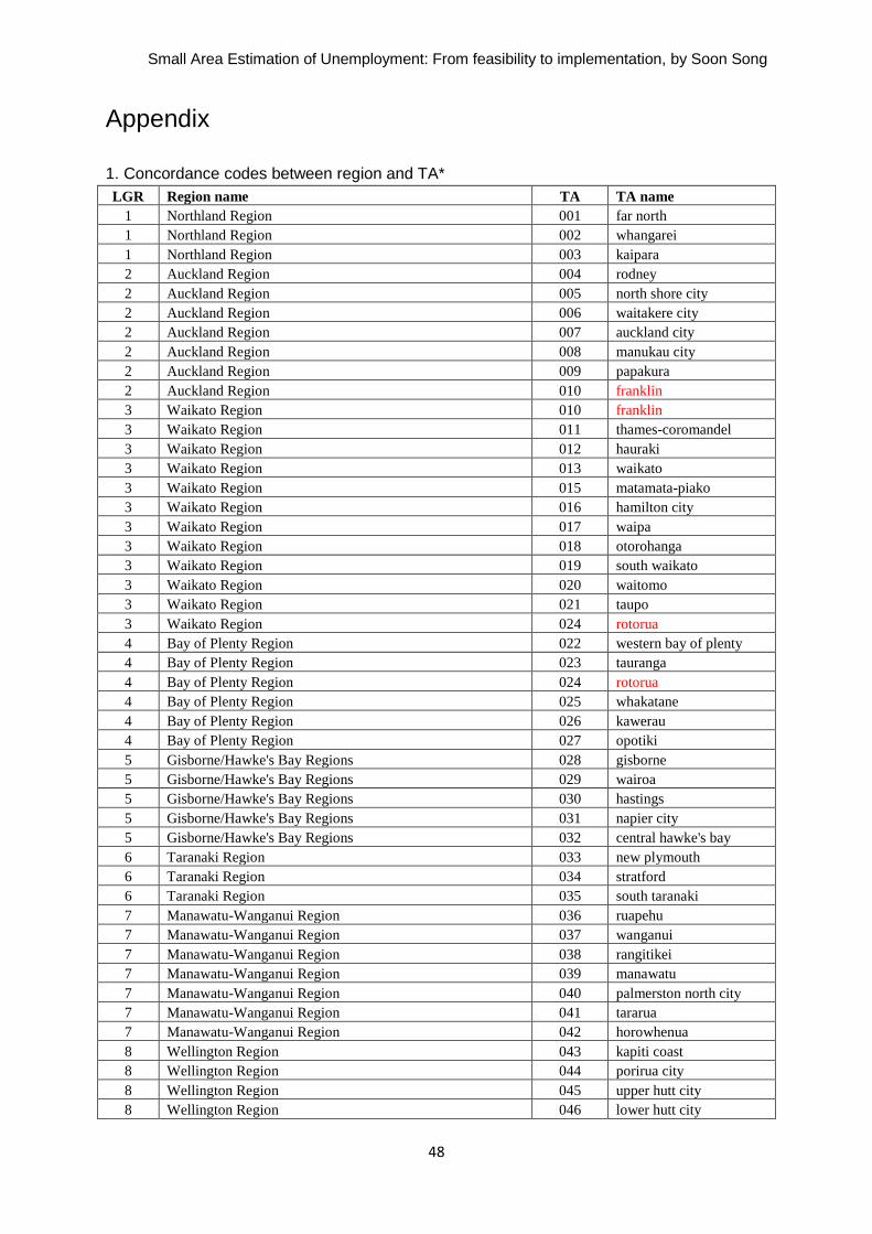
Small Area Estimation of Unemployment: From feasibility to implementation, by Soon Song
48
Appendix 1. Concordance codes between region and TA*
LGR Region name TA TA name
1 Northland Region 001 far north
1 Northland Region 002 whangarei
1 Northland Region 003 kaipara
2 Auckland Region 004 rodney
2 Auckland Region 005 north shore city
2 Auckland Region 006 waitakere city
2 Auckland Region 007 auckland city
2 Auckland Region 008 manukau city
2 Auckland Region 009 papakura
2 Auckland Region 010 franklin
3 Waikato Region 010 franklin
3 Waikato Region 011 thames-coromandel
3 Waikato Region 012 hauraki
3 Waikato Region 013 waikato
3 Waikato Region 015 matamata-piako
3 Waikato Region 016 hamilton city
3 Waikato Region 017 waipa
3 Waikato Region 018 otorohanga
3 Waikato Region 019 south waikato
3 Waikato Region 020 waitomo
3 Waikato Region 021 taupo
3 Waikato Region 024 rotorua
4 Bay of Plenty Region 022 western bay of plenty
4 Bay of Plenty Region 023 tauranga
4 Bay of Plenty Region 024 rotorua
4 Bay of Plenty Region 025 whakatane
4 Bay of Plenty Region 026 kawerau
4 Bay of Plenty Region 027 opotiki
5 Gisborne/Hawke's Bay Regions 028 gisborne
5 Gisborne/Hawke's Bay Regions 029 wairoa
5 Gisborne/Hawke's Bay Regions 030 hastings
5 Gisborne/Hawke's Bay Regions 031 napier city
5 Gisborne/Hawke's Bay Regions 032 central hawke's bay
6 Taranaki Region 033 new plymouth
6 Taranaki Region 034 stratford
6 Taranaki Region 035 south taranaki
7 Manawatu-Wanganui Region 036 ruapehu
7 Manawatu-Wanganui Region 037 wanganui
7 Manawatu-Wanganui Region 038 rangitikei
7 Manawatu-Wanganui Region 039 manawatu
7 Manawatu-Wanganui Region 040 palmerston north city
7 Manawatu-Wanganui Region 041 tararua
7 Manawatu-Wanganui Region 042 horowhenua
8 Wellington Region 043 kapiti coast
8 Wellington Region 044 porirua city
8 Wellington Region 045 upper hutt city
8 Wellington Region 046 lower hutt city

Small Area Estimation of Unemployment: From feasibility to implementation, by Soon Song
49
8 Wellington Region 047 wellington city
8 Wellington Region 048 masterton
8 Wellington Region 050 south wairarapa
9 West Coast/Tasman/Nelson/Marlborough Regions 051 tasman
9 West Coast/Tasman/Nelson/Marlborough Regions 052 nelson city
9 West Coast/Tasman/Nelson/Marlborough Regions 053 marlborough
9 West Coast/Tasman/Nelson/Marlborough Regions 055 buller
9 West Coast/Tasman/Nelson/Marlborough Regions 056 grey
9 West Coast/Tasman/Nelson/Marlborough Regions 057 westland
10 Canterbury Region 058 hurunui
10 Canterbury Region 059 waimakariri
10 Canterbury Region 060 christchurch city
10 Canterbury Region 062 selwyn
10 Canterbury Region 063 ashburton
10 Canterbury Region 064 timaru
10 Canterbury Region 065 mackenzie
10 Canterbury Region 066 waimate
11 Otago Region 068 waitaki
11 Otago Region 069 central otago
11 Otago Region 070 queenstown-lakes
11 Otago Region 071 dunedin city
11 Otago Region 072 clutha
12 Southland Region 073 southland
12 Southland Region 074 gore
12 Southland Region 075 invercargill city
Note: * Excluding TAs are 049 Carterton, 054 Kaikoura and 067 Chatham Islands.