sma5233 particle methods and molecular dynamics lecture 2: physical principles and design issues of...

SMA5233 SMA5233 Particle Methods and Molecular DynamicsParticle Methods and Molecular Dynamics

Lecture 2: Physical Principles and Design Issues of MDLecture 2: Physical Principles and Design Issues of MD

A/P Chen Yu ZongA/P Chen Yu Zong

Tel: 6874-6877Tel: 6874-6877Email: Email: [email protected]@nus.edu.sg

http://http://bidd.nus.edu.sgbidd.nus.edu.sgRoom 08-14, level 8, S16 Room 08-14, level 8, S16

National University of SingaporeNational University of Singapore

22

When is classical mechanics a reasonable approximation?When is classical mechanics a reasonable approximation?

In Newtonian physics, any particle may possess any one of a In Newtonian physics, any particle may possess any one of a continuum of energy values. In quantum physics, the energy is continuum of energy values. In quantum physics, the energy is quantized, not continuous. That is, the system can accomodate quantized, not continuous. That is, the system can accomodate only certain discrete levels of energy, separated by gaps. only certain discrete levels of energy, separated by gaps.

At very low temperatures these gaps are much larger than At very low temperatures these gaps are much larger than thermal energy, and the system is confined to one or just a few thermal energy, and the system is confined to one or just a few of the low-energy states. Here, we expect the `discreteness' of of the low-energy states. Here, we expect the `discreteness' of the quantum energy landscape to be evident in the system's the quantum energy landscape to be evident in the system's behavior. behavior.

As the temperature is increased, more and more states become As the temperature is increased, more and more states become thermally accessible, the `discreteness' becomes less and less thermally accessible, the `discreteness' becomes less and less important, and the system approaches classical behavior. important, and the system approaches classical behavior.

33

When is classical mechanics a reasonable approximation?When is classical mechanics a reasonable approximation?

For a harmonic oscillator, the quantized energies are For a harmonic oscillator, the quantized energies are separated by separated by E=hfE=hf, where , where hh is Planck's constant and is Planck's constant and ff is the frequency of harmonic vibration. is the frequency of harmonic vibration.

Classical behavior is approached at temperatures for Classical behavior is approached at temperatures for which which KKBBT>>hfT>>hf, where , where KKBB is the Boltzmann constant and is the Boltzmann constant and

KKBBTT = 0.596 kcal/mol at 300 K. Setting = 0.596 kcal/mol at 300 K. Setting hfhf = 0.596 = 0.596

kcal/mol yields kcal/mol yields ff = 6.25/ps, or 209cm = 6.25/ps, or 209cm-1-1. So a classical . So a classical treatment will suffice for motions with characteristic times treatment will suffice for motions with characteristic times of a ps or longer at room temperature. of a ps or longer at room temperature.

44

Classical Mechanics - in a NutshellClassical Mechanics - in a Nutshell

Building on the work of Galileo and others, Newton unveiled his Building on the work of Galileo and others, Newton unveiled his laws of motion in 1686. According to Newton: laws of motion in 1686. According to Newton:

1.1. A body remains at rest or in uniform motion (constant velocity A body remains at rest or in uniform motion (constant velocity - both speed and direction) unless acted on by a net external - both speed and direction) unless acted on by a net external force. force.

2.2. In response to a net external force, In response to a net external force, FF, a body of mass , a body of mass mm accelerates with acceleration accelerates with acceleration aa==FF/m/m. .

3.3. If body i pushes on body j with a force If body i pushes on body j with a force FFijij, then body j pushes , then body j pushes

on body i with a force on body i with a force FFjiji=-=-FFijij. .

55

Classical Mechanics - in a NutshellClassical Mechanics - in a Nutshell

For energy-conserving forces, the net force For energy-conserving forces, the net force FFii on particle i is the negative on particle i is the negative

gradient (slope in three dimensions) of the potential energy with respect to gradient (slope in three dimensions) of the potential energy with respect to

particle i's position: particle i's position: FFii= - = - ▼▼iiV(V(RR) where V() where V(RR) represents the potential ) represents the potential

energy of the system as a function of the positions of all N particles, energy of the system as a function of the positions of all N particles, RR. .

In three dimensions, In three dimensions, rrii is the vector of length 3 specifying the position of is the vector of length 3 specifying the position of

the atom, and the atom, and RR is the vector of length specifying all coordinates. In the is the vector of length specifying all coordinates. In the context of simulation, the forces are calculated for energy minimizations context of simulation, the forces are calculated for energy minimizations and molecular dynamics simulations but are not needed in Monte Carlo and molecular dynamics simulations but are not needed in Monte Carlo simulations. simulations.

Classical mechanics is completely deterministic: Given the exact positions Classical mechanics is completely deterministic: Given the exact positions and velocities of all particles at a given time, along with the function , one and velocities of all particles at a given time, along with the function , one can calculate the future (and past) positions and velocities of all particles can calculate the future (and past) positions and velocities of all particles at any other time. The evolution of the system's positions and momenta at any other time. The evolution of the system's positions and momenta through time is often referred to as a trajectory.through time is often referred to as a trajectory.

66

Statistical Mechanics - Calculating Equilibrium Averages Statistical Mechanics - Calculating Equilibrium Averages

According to statistical mechanics, the probability that a given state According to statistical mechanics, the probability that a given state with energy E is occupied in equilibrium at constant particle number N, with energy E is occupied in equilibrium at constant particle number N, volume V, and temperature T (constant , the `canonical' ensemble) is volume V, and temperature T (constant , the `canonical' ensemble) is proportional to exp{-E/ proportional to exp{-E/ KKBBTT}, the `Boltzmann factor.' }, the `Boltzmann factor.'

Probability ~ exp{-E/ Probability ~ exp{-E/ KKBBTT} }

The equilibrium value of any observable O is therefore obtained by The equilibrium value of any observable O is therefore obtained by averaging over all states accessible to the system, weighting each averaging over all states accessible to the system, weighting each state by this factor.state by this factor.

77

Statistical Mechanics - Calculating Equilibrium Averages Statistical Mechanics - Calculating Equilibrium Averages

Classically, a microstate is specified by the positions and velocities (momenta) Classically, a microstate is specified by the positions and velocities (momenta) of all particles, each of which can take on any value. The averaging over states of all particles, each of which can take on any value. The averaging over states in the classical limit is done by integrating over these continuous variables:in the classical limit is done by integrating over these continuous variables:

where the integrals are over all phase space (positions and momenta _) for where the integrals are over all phase space (positions and momenta _) for the N particles in 3 dimensions. the N particles in 3 dimensions.

When all forces (the potential energy V) and the observable O are velocity-When all forces (the potential energy V) and the observable O are velocity-independent, the momentum integrals can be factored and canceled: independent, the momentum integrals can be factored and canceled:

where is the total kinetic energy, where is the total kinetic energy,

and E=K+V. As a result, Monte Carlo simulations and E=K+V. As a result, Monte Carlo simulations

compare V's, not E's.compare V's, not E's.

88

What is molecular mechanics?What is molecular mechanics?

Molecular Mechanics (MM) finds the geometry that corresponds Molecular Mechanics (MM) finds the geometry that corresponds to a minimum energy for the system - a process known as to a minimum energy for the system - a process known as energy minimization. energy minimization.

A molecular system will generally exhibit numerous minima, A molecular system will generally exhibit numerous minima, each corresponding to a feasible conformation. Each minimum each corresponding to a feasible conformation. Each minimum will have a characteristic energy, which can be computed. The will have a characteristic energy, which can be computed. The lowest energy, or global minimum, will correspond to the most lowest energy, or global minimum, will correspond to the most likely conformation. likely conformation.

99

Energy MinimizationEnergy Minimization

Torsion anglesAre 4-body

AnglesAre 3-body

BondsAre 2-body

Non-bondedpair

nonbondedji ij

ji

nonbondedji ij

ij

ij

ijij

torsionsall

anglesall

bondsallb

r

qq

r

R

r

R

nK

K

bbKU

, 0

,

612

20

20

4

2

cos1

2

1

2

1

U is a function of the conformation C of the protein. The problem of “minimizing U” can be stated as finding C such that U(C) is minimum.

1010

Units in force fields

Most force fields use the AKMA (Angstrom – Kcal – Mol – Atomic Mass Unit) unitsystem:

QuantityQuantity AKMA unitAKMA unit Equivalent SIEquivalent SI

EnergyEnergy 1 Kcal/Mol1 Kcal/Mol 4184 Joules4184 Joules

LengthLength 1 Angstrom1 Angstrom 1010-10-10 meter meter

MassMass 1 amu 1 amu (H=1amu)(H=1amu) 1.6605655 101.6605655 10-27-27 Kg Kg

ChargeCharge 1 e1 e 1.6021892 101.6021892 10-19-19 C C

TimeTime 1 unit1 unit 4.88882 104.88882 10-14-14 second second

FrequencyFrequency 1 cm-11 cm-1 18.836 1018.836 101010 rd/s rd/s

1111

Energy MinimizationEnergy Minimization

Local minima:

A conformation X is a local minimum if there exists a domain D in the neighborhood of X such that for all Y≠X in D:

U(X) <U(Y)

Global minimum:

A conformation X is a global minimum if U(X) <U(Y)

for all conformations Y ≠X

1212

Molecular Modeling: Molecular Modeling:

bondednon ijij

ji

ij

ij

ij

ijrra

bondH

bondS

rra

rotationbond

n

eqbendinganglebond

eqrstretchbondatoms

r

qq

r

B

r

AVeV

VeVn

v

krrkm

pH

][])1([

])1([)]cos(1[

2

)(2

1)(

2

1

2

61202)(

0

02)(

0

222

'0

'0

Energy minimization:

Force guided approach:

Initialize: Change atom position: xi -> xi+dxi

Compute potential energy change: V -> V +dV

Determine next movement:

Force: Fxi=-dV/dxi; Fyi=-dV/dyi; Fzi=-dV/dziAtom displacement: dxi=C*FxiNew position: xi=xi+dxi

1313

Notes on computing the energyNotes on computing the energy

nonbondedji ij

ji

nonbondedji ij

ij

ij

ijijNB r

qq

r

R

r

RU

, 0,

612

42

The direct computation of the non bonded interactions involve all pairs of atoms and has a quadratic complexity (O(N2)).This is usually prohibitive for large molecules.

Bonded interactions are local, and therefore their computation has a linearcomputational complexity (O(N), where N is the number of atoms in the molecule considered.

Reducing the computing time: use of cutoff in UNB

1414

ji ij

jiijij

ji ij

ij

ij

ijijijijNB r

qqrS

r

R

r

RrSU

, 0,

612

42

Cutoff schemes for faster energy computation

ij : weights (0< ij <1). Can be used to exclude bonded terms,

or to scale some interactions (usually 1-4)

S(r) : cutoff function.

Three types:

1) Truncation:

br

brrS

0

1)(

b

1515

Cutoff schemes for faster energy computation

2. Switching

a b

br

braryry

ar

rS

0

3)(2)(1

1

)( 2

with 22

22

)(ab

arry

3. Shifting

b

brb

rrS

22

1 1)(

brb

rrS

2

2 1)(

or

1616

The minimizersSome definitions:

Gradient:The gradient of a smooth function f with continuous first and secondderivatives is defined as:

HessianThe n x n symmetric matrix of second derivatives, H(x), is calledthe Hessian:

Ni x

f

x

f

x

fXf ......

1

2

22

1

2

22

1

2

1

2

1

2

21

2

......

...............

......

...............

......

)(

NjNN

Nijii

Nj

x

f

xx

f

xx

f

xx

f

xx

f

xx

f

xx

f

xx

f

x

f

xH

1717

The minimizers

Steepest descent (SD):

The simplest iteration scheme consists of following the “steepestdescent” direction:

Usually, SD methods leads to improvement quickly, but then exhibitslow progress toward a solution.They are commonly recommended for initial minimization iterations,when the starting function and gradient-norm values are very large.

Minimization of a multi-variable function is usually an iterative process, in whichupdates of the state variable x are computed using the gradient, and in some(favorable) cases the Hessian.

Iterations are stopped either when the maximum number of steps (user’s input)is reached, or when the gradient norm is below a given threshold.

)(1 kkk xfxx ( sets the minimum along the line defined by the gradient)

1818

The minimizersConjugate gradients (CG):

In each step of conjugate gradient methods, a search vector pk isdefined by a recursive formula:

The corresponding new position is found by line minimization alongpk:

the CG methods differ in their definition of :

- Fletcher-Reeves:

- Polak-Ribiere

- Hestenes-Stiefel

kkkk pxfp 11

kkkk pxx 1

)()(

)()( 111

kk

kkFRk xfxf

xfxf

)()(

)()()( 111

kk

kkkPRk xfxf

xfxfxf

)()(

)()()(

1

111

kkk

kkkHSk xfxfp

xfxfxf

1919

The minimizersNewton’s methods:

Newton’s method is a popular iterative method for finding the 0 of a one-dimensional function:

k

kkk xg

xgxx

'1

x0x1x2x3

The equivalent iterative scheme for multivariate functions is based on:

kkkkk xfxHxx

11

Several implementations of Newton’s method exist, that avoid computingthe full Hessian matrix: quasi-Newton, truncated Newton, “adopted-basisNewton-Raphson” (ABNR),…

It can be adapted to the minimization of a one –dimensional function, in whichcase the iteration formula is:

k

kkk xg

xgxx

''

'1

2020

What is molecular dynamics simulation?What is molecular dynamics simulation?

Molecular DynamicsMolecular Dynamics (MD) applies the laws of (MD) applies the laws of classical mechanics to compute the motion of the classical mechanics to compute the motion of the particles in a molecular system.particles in a molecular system.

Simulation that shows how the atoms in the system Simulation that shows how the atoms in the system move with timemove with time

Typically on the nanosecond timescaleTypically on the nanosecond timescale

Atoms are treated like hard balls, and their motions Atoms are treated like hard balls, and their motions are described by Newton’s laws.are described by Newton’s laws.

2121

Molecular dynamics simulations generate information at the microscopic level, including atomic positions and velocities.

The conversion of this microscopic information to macroscopic observables such as pressure, energy, heat capacities, etc., requires statistical mechanics.

MD Simulation

Microscopic information

Macroscopic properties

Statistical Mechanics

What is molecular dynamics simulation?What is molecular dynamics simulation?

2222

Characteristic protein motionsCharacteristic protein motions

Type of motionType of motion TimescaleTimescale AmplitudeAmplitude

Local:Local:

bond stretchingbond stretching

angle bendingangle bending

methyl rotationmethyl rotation

0.01 ps0.01 ps

0.1 ps0.1 ps

1 ps1 ps

< 1 < 1 ÅÅ

Medium scaleMedium scale

loop motionsloop motions

SSE formationSSE formation ns – ns – ss 1-5 1-5 ÅÅ

GlobalGlobal

protein tumblingprotein tumbling

(water tumbling)(water tumbling)

protein foldingprotein folding

20 ns20 ns

(20 ps)(20 ps)

ms – hrsms – hrs

> 5 > 5 ÅÅ

Periodic (harmonic)

Random (stochastic)

2323

Molecular Dynamics Simulation

Molecule: (classical) N-particle system

Newtonian equations of motion: )r(Frdt

dm iii

2

2

)()( rVrF ii

)r,...,r(r N

1with

Integrate numerically via the „leapfrog“ scheme:

(equivalent to the Verlet algorithm)

with

Δt 1fs!

2424

How do you run a MD simulation?How do you run a MD simulation?Get the initial configurationGet the initial configuration

From x-ray crystallography or NMR spectroscopy (PDB)From x-ray crystallography or NMR spectroscopy (PDB)

Assign initial velocitiesAssign initial velocities

At thermal equilibrium, the expected value of the kinetic energy of the At thermal equilibrium, the expected value of the kinetic energy of the system at temperature T is:system at temperature T is:

This can be obtained by assigning the velocity components vi from a This can be obtained by assigning the velocity components vi from a random Gaussian distributionrandom Gaussian distribution

with mean 0 and standard deviation (with mean 0 and standard deviation (kkBBT/mT/mii):):

TkNvmE B

N

iiikin )3(

2

1

2

1 3

1

2

i

Bi m

Tkv 2

2525

For each time step:

Compute the force on each atom:

Solve Newton’s 2nd law of motion for each atom, to get newcoordinates and velocities

Store coordinates

Stop

How do you run a MD simulation?How do you run a MD simulation?

X

EXEXF

)()(

)(XFXM

X: cartesian vector of the system

M diagonal mass matrix

.. means second order differentiation with respect to time

Newton’s equation cannot be solved analytically: Use stepwise numerical integration

2626

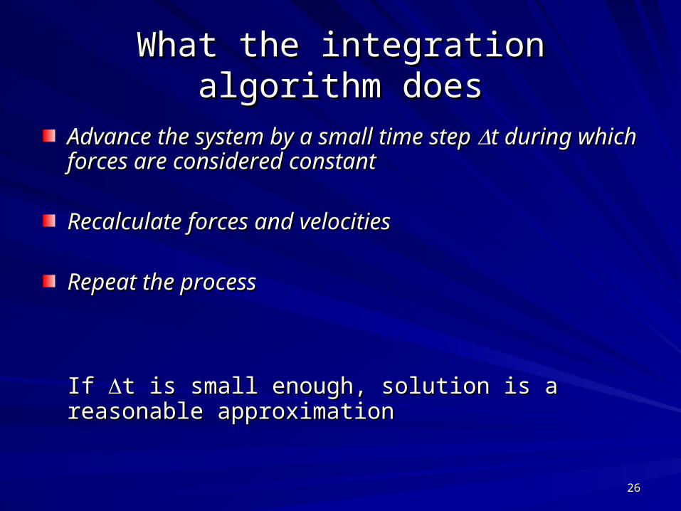
What the integration algorithm doesWhat the integration algorithm does

Advance the system by a small time step Advance the system by a small time step t during which t during which forces are considered constantforces are considered constant

Recalculate forces and velocitiesRecalculate forces and velocities

Repeat the processRepeat the process

If If t is small enough, solution is a reasonable t is small enough, solution is a reasonable approximationapproximation

2727

Choosing a time step Choosing a time step tt

Not too short so that conformations are efficiently sampledNot too short so that conformations are efficiently sampled

Not too long to prevent wild fluctuations or system ‘blow-Not too long to prevent wild fluctuations or system ‘blow-up’ up’

An order of magnitude less than the fastest motion is idealAn order of magnitude less than the fastest motion is ideal– Usually bond stretching is the fastest motion: Usually bond stretching is the fastest motion: C-H is ~10fs so use time step of C-H is ~10fs so use time step of 1fs1fs

– Not interested in these motions? Not interested in these motions? Constrain these bonds and double the time stepConstrain these bonds and double the time step

2828

Molecular Dynamics EnsemblesMolecular Dynamics Ensembles

The method discussed above is appropriate for the The method discussed above is appropriate for the micro-canonical ensemble: constant N (# of particles) V micro-canonical ensemble: constant N (# of particles) V (volume) and E(volume) and ETT (total energy = E + E (total energy = E + Ekinkin))

In some cases, it might be more appropriate to simulate In some cases, it might be more appropriate to simulate under constant Temperature (T) or constant Pressure under constant Temperature (T) or constant Pressure (P):(P):– Canonical ensemble: NVTCanonical ensemble: NVT– Isothermal-isobaric: NPTIsothermal-isobaric: NPT– Constant pressure and enthalpy: NPHConstant pressure and enthalpy: NPH

How do you simulate at constant temperature and pressure?How do you simulate at constant temperature and pressure?

2929

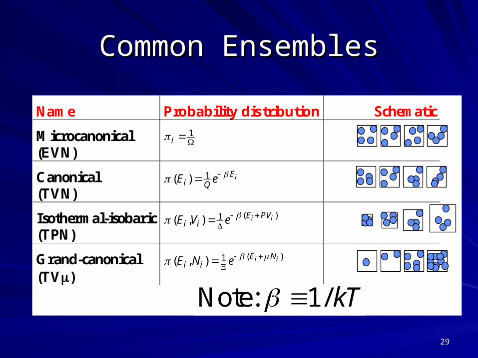
Common EnsemblesCommon Ensembles

Name Probability distribution Schematic

Microcanonical (EVN)

1i

Canonical (TVN)

1( ) iEi Q

E e

Isothermal-isobaric (TPN)

( )1( , ) i iE PVi iE V e

Grand-canonical (TV)

( )1( , ) i iE Ni iE N e

Note: 1/ kT

3030

MD in different thermodynamic ensembleMD in different thermodynamic ensemble

MD naturally samples the MD naturally samples the NVENVE (microcanonical (microcanonical ensemble): this is not very useful for most ensemble): this is not very useful for most applications.applications.

• More useful ensembles include:– Canonical (NVT): requires the particles to interact

with a thermostat– Isobaric-Isothermal (NPT): requires the particles to

interact with a thermostat and a baristat

3131

TemperatureTemperature

Thermodynamics definitionThermodynamics definition

,

1

1ln ( , , )

V N

S

T E

E V NkT E

2

1

1 2Ni

i

kT KNd m Nd

p

Measuring TMeasuring T

3232

Canonical (NVT)Canonical (NVT)Several possible approachesSeveral possible approaches– Berendsen MethodBerendsen Method (velocities are rescaled (velocities are rescaled

deterministically after each step so that the system deterministically after each step so that the system is forced towards the desired temperature)is forced towards the desired temperature)

– Extended Lagrangians (Nose and Nose-Hoover: the thermal reservoir is considered an integral part of the system and it is represented by an additional degree of freedom: set of deterministic equations that give sampling in NVT)

– Stochastic collisions (Anderson: a random particle’s velocity is reassigned by random selection from the Maxwell-Boltzmann distribution at set intervals)

3333

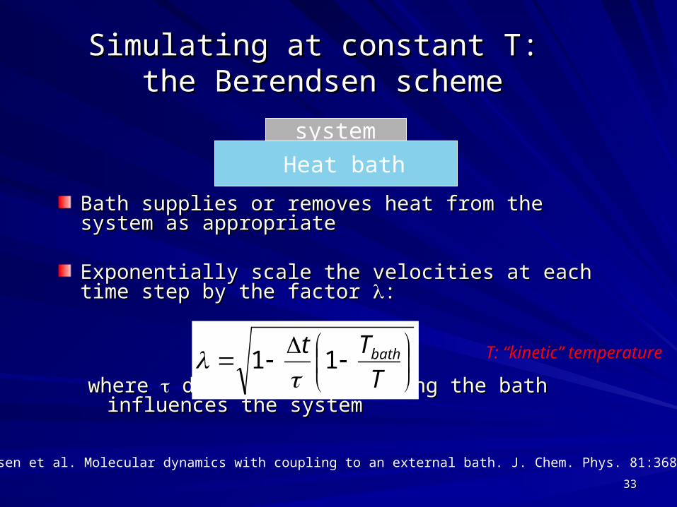
Bath supplies or removes heat from the system as Bath supplies or removes heat from the system as appropriateappropriate

Exponentially scale the velocities at each time step by the Exponentially scale the velocities at each time step by the factor factor ::

where where determines how strong the bath influences the determines how strong the bath influences the systemsystem

Simulating at constant T: Simulating at constant T: the Berendsen scheme the Berendsen scheme

system

Heat bath

Berendsen et al. Molecular dynamics with coupling to an external bath. J. Chem. Phys. 81:3684 (1984)

T

Tt bath11

T: “kinetic” temperature

3434

Simulating at constant P: Simulating at constant P: Berendsen schemeBerendsen scheme

Couple the system to a pressure bathCouple the system to a pressure bath

Exponentially scale the volume of the simulation box at Exponentially scale the volume of the simulation box at each time step by a factor each time step by a factor ::

where where : isothermal compressibility : isothermal compressibility PP : coupling constant : coupling constant

system

pressure bath

Berendsen et al. Molecular dynamics with coupling to an external bath. J. Chem. Phys. 81:3684 (1984)

bathP

PPt

1

N

iiikin FxE

vP

13

2where

: volumexi: position of particle iFi : force on particle i

3535

Nose-Hoover ThermostatNose-Hoover Thermostat

22

1

( )( ) ln

2 2

NNi i

Nosei

m QL U sgks T

s

r

r

2i i i

i

s

Lm s

Lp Qs

s

p rr

Introduce a new coordinate, s, representing reservoir in the Lagrangian

With momenta: Q=effective mass associatedwith s

g is a parameter we will fixlater

3636

Extended-system Hamiltonian:Extended-system Hamiltonian:

2 2

21

( ) ln22

NNi s

Nosei i

pH U gkT s

Qm s p

r

VTN

Nose

rpArs

pAtr

ts

tpdtAA ,',)(,

)(

)(lim

0

With p’=p/s

it can be shown that the molecular positions and it can be shown that the molecular positions and momenta follow a canonical (NVT) distribution if g = momenta follow a canonical (NVT) distribution if g = 3N+13N+1


3737

s can be interpreted as a scaling factor of the time steps can be interpreted as a scaling factor of the time step– ttrealreal = t = tsimsim//ss– since since ss varies during the simulation, each “true” time step varies during the simulation, each “true” time step

is of varying lengthis of varying length

Real and virtual variables are related by:

s

tt

sss

pp

rr

'

'

'

'Nose-Hoover ThermostatNose-Hoover Thermostat

3838

Scaled-variables Scaled-variables equations of motionequations of motion– constant simulation constant simulation tt– fluctuating real fluctuating real tt

2

21

1

ii

i i

i ii

s

s

Ni

si i

H

m s

H

H ps

p Q

H pp gkT

s s m s

pr

p

p Fr

Real-variables equation Real-variables equation of motion (here, I haveof motion (here, I have

Dropped the prime)Dropped the prime)

1

( / ) 1

ii

i

si i i

s

Ns i

ii

m

sp

Q

s sp

s Q

sp Q pgkT

t Q m

pr

p F p

From the Hamiltonian, can derive the equations of motion for the virtual variables p, r and t.


3939

IMPLEMENTATION

Simplify expression (Nose-Hoover) by introducing a thermodynamicFriction coefficient:

Q

ps s''

1

1

ii

i

i i i

Ni

ii

m

s

s

pgkT

Q m

pr

p F p

So equations of motions (dropping the prime):

(g=3N)

4040

An experiment is usually made on a macroscopic sample that contains an extremely large number of atoms or molecules sampling an enormous number of conformations. In statistical mechanics, averages corresponding to experimental observables are defined in terms of ensemble averages;

4141

Thermodynamic (Ensemble) average: average over all points in phase space at a Single time

Dynamic average: average over a single point in phase space atAll times

Ergodic hypothesis: for infinitely long trajectory, thermo average= Dynamic average

ensembletimeAA

A large number of observations made on a single system at N arbitrary instants in time have the same statistical properties as observing N arbitrarily chosen systems at the same time.

AVERAGES

4242

To get a thermo average, need to know the probability of finding the system at each point (state) in phase space.

Tk

prH

Qpr

B

NNNN ),(

exp1

,

Tk

prHdrdpQ

B

NNNN ),(

exp

Probability density

Partition function

Ensemble (thermodynamic) average of observable A(rN,pN):

NNNNNNens

prprAdrdpA ,,

4343

In an MD simulation, we determine a time average of A, which is expressed as

where is the simulation time, M is the number of time steps in the simulation and A(pN,rN) is the instantaneous value of A.

4444

THERMODYNAMIC PROPERTIES FROM MD SIMULATIONS

Thermodynamic (equilibrium) averages can be calculated via time averaging:

)(1

1

N

iitA

NA

Examples:

)(1

1

N

iitU

NU Average potential energy

i

N

iji

M

jj

j tvtvm

NK

1 1 2

1Average kinetic energy

4545

Other quantities obtained from MD: Other quantities obtained from MD: Heat CapacityHeat Capacity

Expressed in terms of fluctuations in the energyExpressed in terms of fluctuations in the energy

22

2, ,

2

( )

1

( )

vV N V N

N N E

E AC k

T

k dr dp EeQ

22 2vC k E E

4646

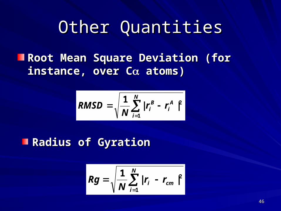
Other QuantitiesOther Quantities

Root Mean Square Deviation (for instance, Root Mean Square Deviation (for instance, over Cover C atoms) atoms)

N

i

Ai

Bi rr

NRMSD

1

2||1

Radius of GyrationRadius of Gyration

N

icmi rr

NRg

1

2||1

4747

From PDB orXtal

Relieve local stresses,Relax bond length/angle distortions

velocities (vx, vy,vz) are randomly

assigned according to a Maxwellian distribution,

P(vi)dv = (m/2pikBT)1/2 exp[ -mv2/2kBT ]dv

to overcome “hot spots” due toInitial high velocities

T(t) = (1/kB(3N-n)) (mivi2)

Scale velocities by (T'/T(t))1/2 to get newtemperatureT

4848

Types of MD SystemsTypes of MD Systems

Empirical PotentialsEmpirical Potentials

Empirical potentials either ignore quantum mechanical effects, or attempt to capture Empirical potentials either ignore quantum mechanical effects, or attempt to capture quantum effects in a limited way through entirely empirical equations. Parameters in quantum effects in a limited way through entirely empirical equations. Parameters in the potential are fitted against known physical properties of the atoms being the potential are fitted against known physical properties of the atoms being simulated, such as elastic constants and lattice parameters.simulated, such as elastic constants and lattice parameters.

Empirical potentials can further be subcategorized into pair potentials, and many-Empirical potentials can further be subcategorized into pair potentials, and many-body potentialsbody potentials– Pair potentials: the total potential energy of a system can be calculated from the sum of Pair potentials: the total potential energy of a system can be calculated from the sum of

energy contributions from pairs of atoms.energy contributions from pairs of atoms.– Many-body potentials: the potential energy cannot be found by a sum over pairs of atoms. Many-body potentials: the potential energy cannot be found by a sum over pairs of atoms.

Tersoff Potential involves a sum over groups of three atoms, with the angles between the atoms Tersoff Potential involves a sum over groups of three atoms, with the angles between the atoms being an important factor in the potential.being an important factor in the potential.

Tight-Binding Second Moment Approximation (TBSMA), the electron density of states in the Tight-Binding Second Moment Approximation (TBSMA), the electron density of states in the region of an atom is calculated from a sum of contributions from surrounding atoms, and the region of an atom is calculated from a sum of contributions from surrounding atoms, and the potential energy contribution is then a function of this sum.potential energy contribution is then a function of this sum.

4949


Semi-Empirical PotentialsSemi-Empirical Potentials

Semi-empirical potentials make use of the matrix representation from Semi-empirical potentials make use of the matrix representation from quantum mechanics. However, the values of the matrix elements are quantum mechanics. However, the values of the matrix elements are found through empirical formulae that estimate the degree of overlap of found through empirical formulae that estimate the degree of overlap of specific atomic orbitals. The matrix is then diagonalized to determine specific atomic orbitals. The matrix is then diagonalized to determine the occupancy of the different atomic orbitals, and empirical formulae the occupancy of the different atomic orbitals, and empirical formulae are used once again to determine the energy contributions of the are used once again to determine the energy contributions of the orbitals.orbitals.

There are a wide variety of semi-empirical potentials, known as tight-There are a wide variety of semi-empirical potentials, known as tight-binding potentials, which vary according to the atoms being modeled.binding potentials, which vary according to the atoms being modeled.

5050


Ab-initio (First Principles) MethodsAb-initio (First Principles) Methods

Ab-initio (first principles) methods use full quantum-mechanical formula Ab-initio (first principles) methods use full quantum-mechanical formula to calculate the potential energy of a system of atoms or molecules. to calculate the potential energy of a system of atoms or molecules. This calculation is usually made "locally", i.e., for nuclei in the close This calculation is usually made "locally", i.e., for nuclei in the close neighborhood of the reaction coordinate. Although various neighborhood of the reaction coordinate. Although various approximations may be used, these are based on theoretical approximations may be used, these are based on theoretical considerations, not on empirical fitting. Ab-Initio produce a large considerations, not on empirical fitting. Ab-Initio produce a large amount of information that is not available from the empirical methods, amount of information that is not available from the empirical methods, such as density of states information.such as density of states information.

Perhaps the most famous ab-initio package is the Car-Parrinello Perhaps the most famous ab-initio package is the Car-Parrinello Molecular Dynamics (CPMD) package based on the density functional Molecular Dynamics (CPMD) package based on the density functional theory..theory..

5151


Coarse-Graining: "Reduced Representations"Coarse-Graining: "Reduced Representations"

The earliest MD simulations on proteins, lipids and nucleic acids The earliest MD simulations on proteins, lipids and nucleic acids generally used "united atoms", which represents the lowest level of generally used "united atoms", which represents the lowest level of coarse graining. For example, instead of treating all four atoms of a coarse graining. For example, instead of treating all four atoms of a methyl group explicitly (or all three atoms of a methylene group), one methyl group explicitly (or all three atoms of a methylene group), one represents the whole group with a single pseudoatom. This represents the whole group with a single pseudoatom. This pseudoatom must, of course, be properly parameterized so that its van pseudoatom must, of course, be properly parameterized so that its van der Waals interactions with other groups have the proper distance-der Waals interactions with other groups have the proper distance-dependence. Similar considerations apply to the bonds, angles, and dependence. Similar considerations apply to the bonds, angles, and torsions in which the pseudoatom participates. In this kind of united torsions in which the pseudoatom participates. In this kind of united atom representation, one typically eliminates all explicit hydrogen atom representation, one typically eliminates all explicit hydrogen atoms except those that have the capability to participate in hydrogen atoms except those that have the capability to participate in hydrogen bonds ("polar hydrogens").bonds ("polar hydrogens").

5252


Coarse-Graining: "Reduced Representations"Coarse-Graining: "Reduced Representations"

When coarse-graining is done at higher levels, the accuracy of the dynamic When coarse-graining is done at higher levels, the accuracy of the dynamic description may be less reliable. But very coarse-grained models have been used description may be less reliable. But very coarse-grained models have been used successfully to examine a wide range of questions in structural biology. Following successfully to examine a wide range of questions in structural biology. Following are just a few examples.are just a few examples.– protein folding studies are often carried out using a single (or a few) pseudoatoms per protein folding studies are often carried out using a single (or a few) pseudoatoms per

amino acid; amino acid; – DNA supercoiling has been investigated using 1-3 pseudoatoms per basepair, and at DNA supercoiling has been investigated using 1-3 pseudoatoms per basepair, and at

even lower resolution; even lower resolution; – Packaging of double-helical DNA into bacteriophage has been investigated with models Packaging of double-helical DNA into bacteriophage has been investigated with models

where one pseudoatom represents one turn (about 10 basepairs) of the double helix; where one pseudoatom represents one turn (about 10 basepairs) of the double helix; – RNA structure in the ribosome and other large systems has been modeled with one RNA structure in the ribosome and other large systems has been modeled with one

pseudoatom per nucleotide. pseudoatom per nucleotide. – The parameterization of these very coarse-grained models must be done empirically, The parameterization of these very coarse-grained models must be done empirically,

by matching the behavior of the model to appropriate experimental data.by matching the behavior of the model to appropriate experimental data.

5353

Electrostatics and the `Generalized Born' Solvent Model Electrostatics and the `Generalized Born' Solvent Model

All problems in electrostatics boil down to the solution of a single All problems in electrostatics boil down to the solution of a single equation, Poisson's equation: equation, Poisson's equation:

where is the Laplacian operator, where is the Laplacian operator, is the electrostatic potential, is the electrostatic potential, is is the charge density (total charge per unit volume including all `free' and the charge density (total charge per unit volume including all `free' and `polarization' charges), and `polarization' charges), and 00 is the permittivity of free space. In is the permittivity of free space. In

Cartesian (xyz) coordinates, Cartesian (xyz) coordinates,

The electrostatic potential at a given point in space is the potential The electrostatic potential at a given point in space is the potential energy per unit charge that a test charge would have if positioned at energy per unit charge that a test charge would have if positioned at that point in the that point in the electric fieldelectric field EE specified by specified by : :

5454

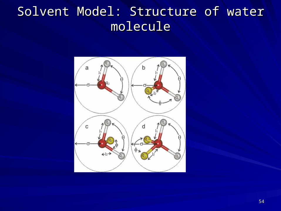
Solvent Model: Structure of water moleculeSolvent Model: Structure of water molecule

5555

Solvent Model: Estimate the average Solvent Model: Estimate the average distance between water moleculesdistance between water molecules

32923_1 10*0.3

10.022,6m

VV mole

molecule

353

3

10*8.110

10*18/m

dengsity

MoleMassVmole

AL

mL

1.3

10*0.3 3293

5656

Solvent Model: Layout of water moleculeSolvent Model: Layout of water molecule

Divide the cubic evenly Divide the cubic evenly into meshes, according to into meshes, according to the distances between the distances between water moleculeswater moleculesPlace oxygen atom of Place oxygen atom of each water molecule on each water molecule on the node of the mesh, the node of the mesh, generate random generate random direction for hydrogen direction for hydrogen atoms.atoms.

5757

Add-in a Molecule (Nano-tube)Add-in a Molecule (Nano-tube)

5858

MD Simulation ResultMD Simulation Result

5959

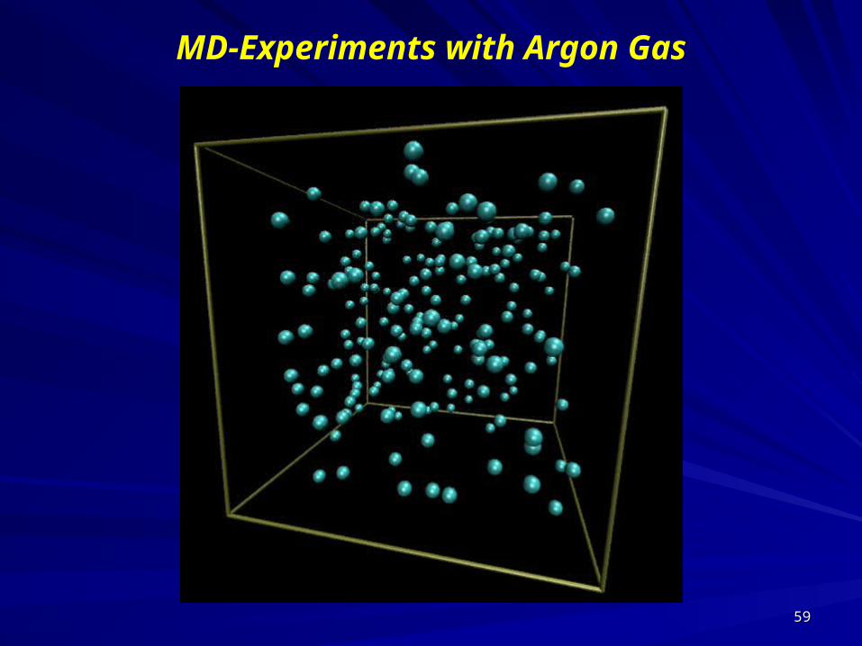
MD-Experiments with Argon Gas

6060

Role of environment - solventRole of environment - solvent

explicit

or

implicit?

box

or

droplet?

6161

periodic boundary conditions

and the minimum image convention

Surface (tension) effects?

6262

Proteins jump between many, hierarchically ordered „conformational substates“

H. Frauenfelder et al., Science 229 (1985) 337

6363

Molecular Dynamics Simulations

• External coupling: Temperature (potential truncation, integration errors) Pressure (density equilibration) System translation/rotation

• Analysis

Energies (individual terms, pressure, temperature) Coordinates (numerical analysis, visual inspection!) Mechanisms

6464


Design Constraints:

• Design of a molecular dynamics simulation can often encounter limits of computational power. Simulation sizes and time duration must be selected so that the calculation can finish within a useful time period.

• The simulation's time duration is dependent on the time length of each timestep, between which forces are recalculated. The timestep must be chosen small enough to avoid discretization errors, and the number of timesteps, and thus simulation time, must be chosen large enough to capture the effect being modeled without taking an extraordinary period of time.

• The simulation size must be large enough to express the effect without the boundary conditions disrupting the behavior. Boundary constraints are often treated by choosing fixed conditions at the boundary, or by choosing periodic boundary conditions in which one side of the simulation loops back to the opposite side.

6565

Design Constraints:

• The scalability of the simulation with respect to the number of molecules is usually a significant factor in the range of simulation sizes which can be simulated in a reasonable time period.

• In Big O notation, common molecular dynamics simulations usually scale by either O(nlog(n)), or with good use of neighbour tables, O(n), with n as the number of molecules


sma5233 particle methods and molecular dynamics lecture 2: physical principles and design issues of...

Documents