slide -5 solute transport - institut teknologi bandung · tl 3106 pencemaran tanah (soil...

TL 3106

PENCEMARAN TANAH

(SOIL CONTAMINATION)

Pengajar: Ir. Yuniati, MT, MSc, PhD

PRODI TEKNIK LINGKUNGAN Fakultas Teknik Sipil dan Lingkungan

Institut Teknologi Bandung

SLIDE -5

Solute Transport ( sumber : Fetter )

I. Movement of contaminants Mechanism of contaminant movement:

A. Dispersion

B. Advection

C. Diffusion

D. Retardation

Dispersion is the process of mechanical mixing that takes place in porous media as a result of the movement of fluids through the pore space.

Hydrodynamic dispersion is a term used to include both diffusion and dispersion.

Mechanical dispersion is caused by local variations in the velocity field on scales ranging from microscopic through macroscopic to megascopic.

Variations in hydraulic conductivity due to lithological heterogeneities are the main sources of velocity variations.

A. Dispersion

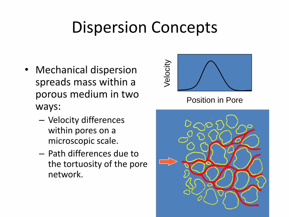
Dispersion Concepts

• Mechanical dispersion spreads mass within a porous medium in two ways: – Velocity differences

within pores on a microscopic scale.

– Path differences due to the tortuosity of the pore network.

Position in Pore

Ve

locity

Dispersion: spreading of plumes

*water flowing through a porous medium takes different routes

*important components: longitudinal & transverse dispersion

velocity dependent, so equivalent only for very slow flow

•D* = 10-5 m2/day. (D* = diffusion constant)

• aL = 0.1m/day (dispersion constant, longitudinal).

• ar = 0.001m/day (dispersion constant, transverse).

•( aL)(Vx) + D* = DL ---> longitudinal

•( aT)(Vz) + D* = DT ---> transverse

Factors causing pore-scale longitudinal dispersion

Figure 10.8 Fetter, Applied Hydrogeology 4th Edition

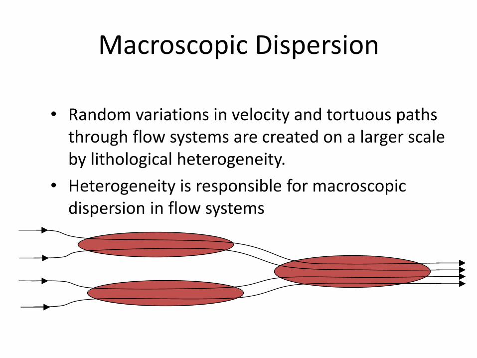
Macroscopic Dispersion

• Random variations in velocity and tortuous paths through flow systems are created on a larger scale by lithological heterogeneity.

• Heterogeneity is responsible for macroscopic dispersion in flow systems

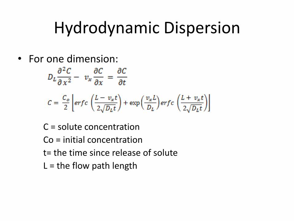
Hydrodynamic Dispersion

• For one dimension:

C = solute concentration

Co = initial concentration

t= the time since release of solute

L = the flow path length

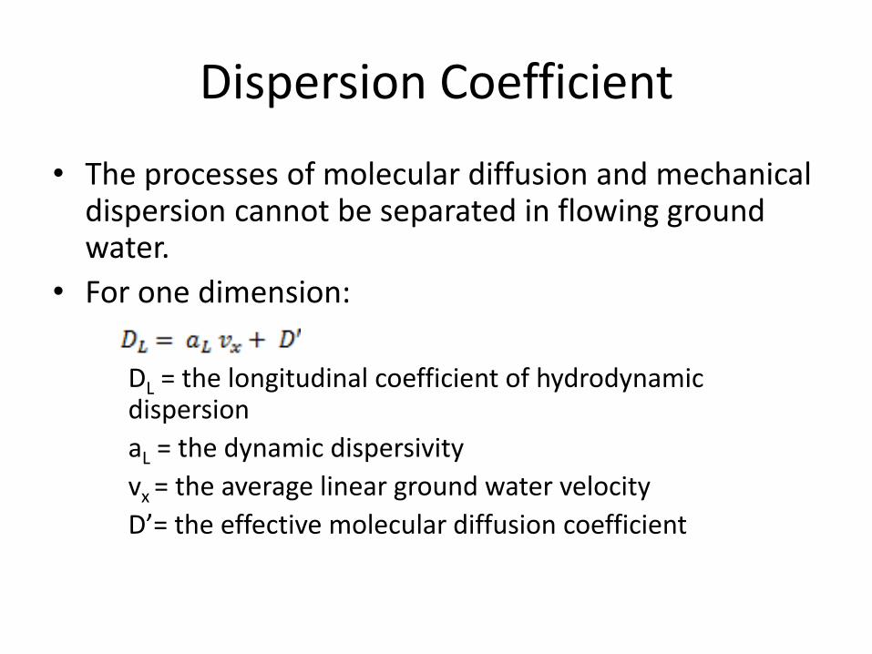
Dispersion Coefficient

• The processes of molecular diffusion and mechanical dispersion cannot be separated in flowing ground water.

• For one dimension:

DL = the longitudinal coefficient of hydrodynamic dispersion

aL = the dynamic dispersivity

vx = the average linear ground water velocity

D’= the effective molecular diffusion coefficient

Dispersion and Scale (Scale effect)

• Mechanical dispersion is also caused by heterogeneities in the aquifer.

• The greater the distance over dispersivity is measured, the greater the value that is observed

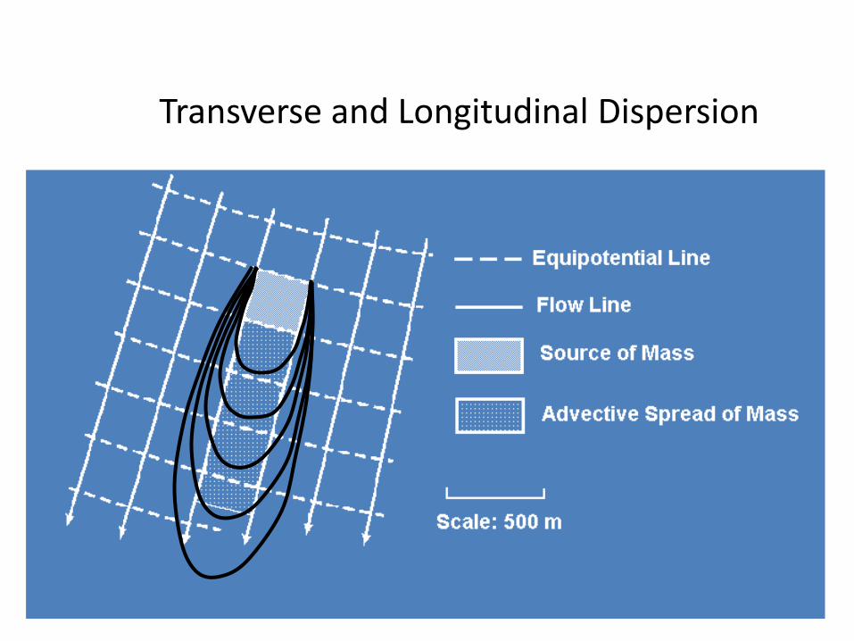
Transverse and Longitudinal Dispersion

Peclet Number

• D/Dd is a convenient ratio that normalizes dispersion coefficients by dividing by the diffusion coefficient.

• v.dm /Dd is called the Peclet Number (NPE) a dimensionless number that expresses the advective to diffusive transport ratio.

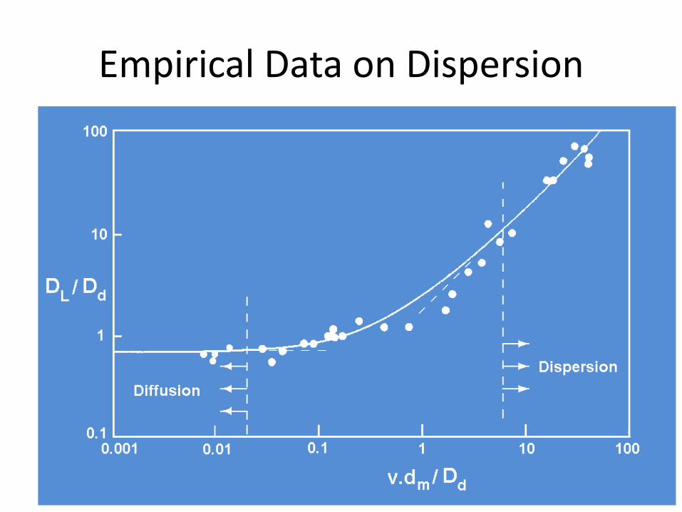
Empirical Data on Dispersion

Transport Regimes

• For NPE < 0.02

diffusion dominates

• For 0.02 > NPE < 8

diffusion and mechanical dispersion

• For NPE > 8

mechanical dispersion dominates

Some authors place the boundaries at 0.01 and 4 rather than 0.02 and 8

Velocity Proportionality

• For values of NPE > 8 the longitudinal (and transverse) dispersion coefficient (DL) is proportional to the advective velocity (v).

• This result has been generalized to describe dispersion both on microscopic and megascopic scales.

• Tranverse dispersion coefficients (DT) are typically around 0.1DL for NPE > 100 although values as low as 0.0 1DL have been reported.

Dispersivity

• Dispersion coefficients may be written:

DL = aL.v and DT = aT.v

where aL and aT are called the dispersivities.

• Dispersivities have units of length and are characteristic properties of porous media.

Dispersion and Scale • Most knowledge of dispersion has been gleaned

from experimental work at the microscopic scale.

• A review of many dispersivity measurements (Gelhar et al, 1992) gave values for aL spanning almost six orders of magnitude.

• Microscopic scale dispersivities as a result of velocity changes on the pore scale are about two orders of magnitude smaller than macroscopic dispersivities arising from heterogeneity in hydraulic conductivity.

Fickian Model

• Hydrodynamic dispersion occurs due to a combination of molecular diffusion and mechanical dispersion.

• A Fickian dispersion model implies that mass transport is proportional to the concentration gradient and in the direction of the concentration gradient (just like Fick’s law for diffusion).

• Using such a model, we treat dispersion in a way fully analogous to diffusion (even though the processes of diffusion and dispersion are quite different).

B. Advection: horizontal velocity


Advective transport and the influence of dispersion and diffusion on “breakthrough” of a solute

• Advection is mass transport due simply to the flow of the water in which the mass is carried.

• The direction and rate of transport coincide with that of the groundwater flow.

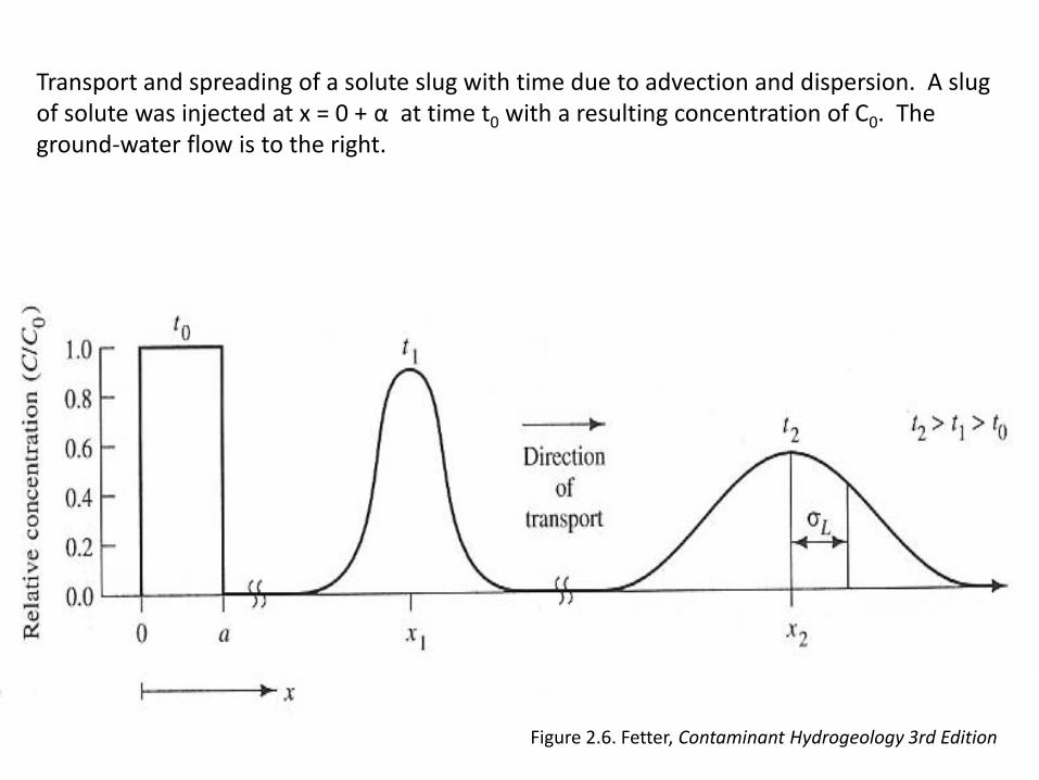
Transport and spreading of a solute slug with time due to advection and dispersion. A slug of solute was injected at x = 0 + α at time t0 with a resulting concentration of C0. The ground-water flow is to the right.

Figure 2.6. Fetter, Contaminant Hydrogeology 3rd Edition

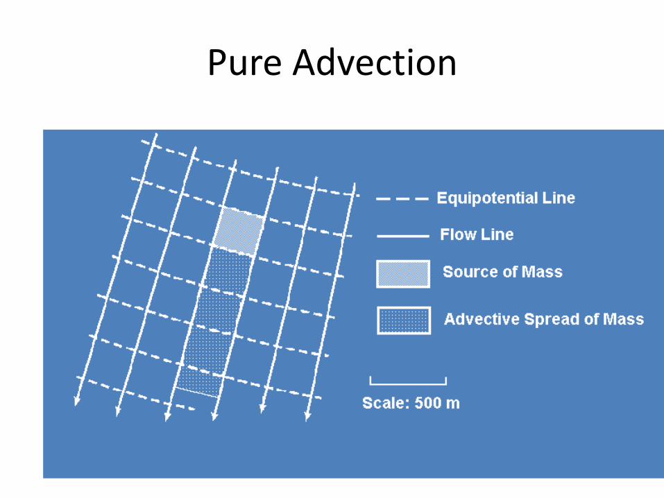
Pure Advection

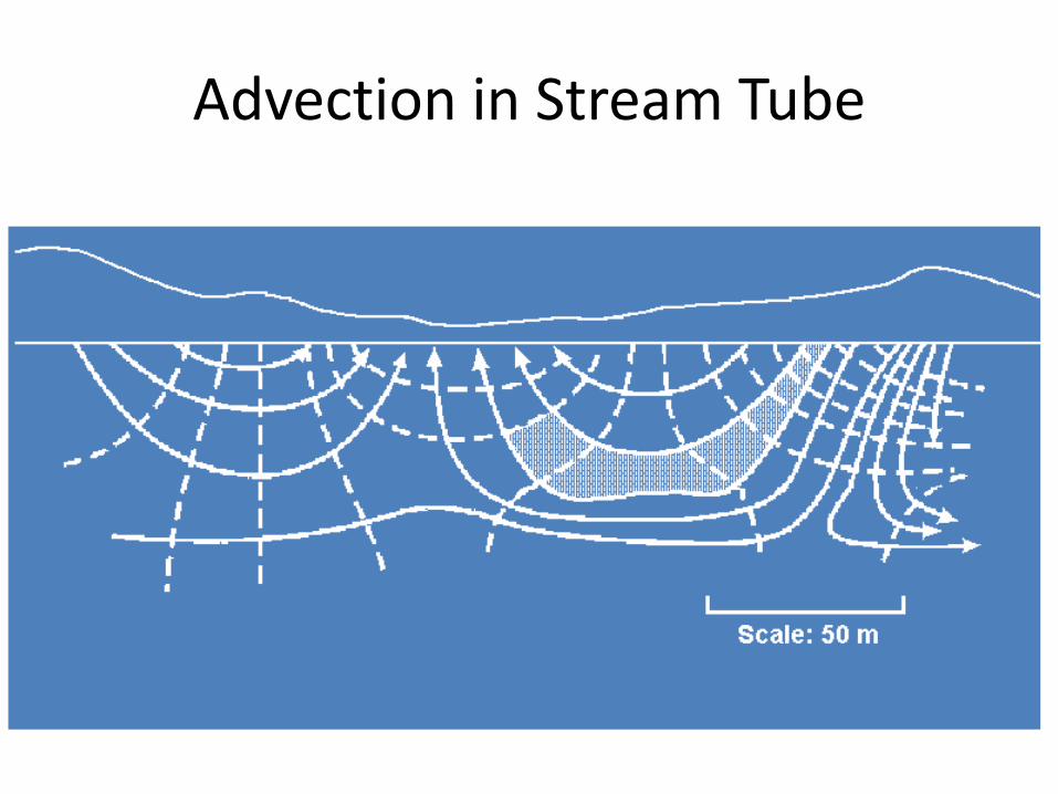
Advection in Stream Tube

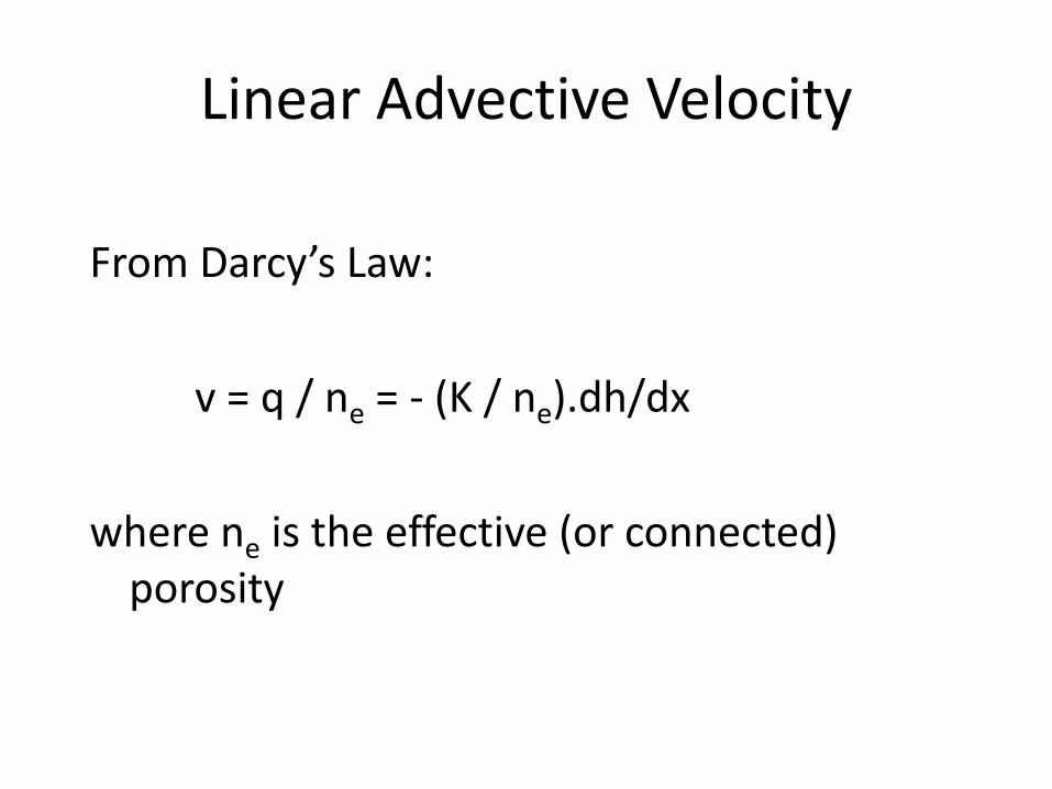
Linear Advective Velocity

From Darcy’s Law:

v = q / ne = - (K / ne).dh/dx

where ne is the effective (or connected) porosity

Fractured Rocks and Clays

• In fractured rocks, the effective porosity (ne) can be very small implying relatively high advective velocities.

• In clays and shales, effective porosity can also be very low and high advective velocities might be expected but there are other factors at work.

Deviations from Advective Velocity

• Electrical charges on clay mineral surfaces can force anions to the centre of pores where velocities are highest.

• Anions can then travel faster than the advective velocity.

• Cations are attracted by the clay mineral surface charge and can be retarded (travel slower than the advective velocity).

• Bi-polar water molecules can similarly be retarded giving rise to osmotic and membrane filtration effects.

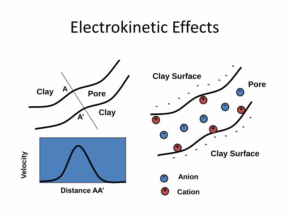
Electrokinetic Effects

Distance AA’

Ve

locit

y

A

A’

Pore Clay

Clay

Clay Surface

Clay Surface

-

- - -

- - -

-

-

-

- - -

- - -

-

-

Pore

- -

-

-

-

+

+

+

+

+

-

+

Anion

Cation

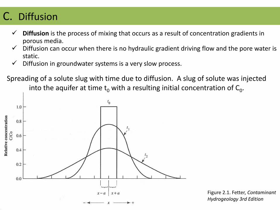
C. Diffusion

Spreading of a solute slug with time due to diffusion. A slug of solute was injected into the aquifer at time t0 with a resulting initial concentration of C0.


Diffusion is the process of mixing that occurs as a result of concentration gradients in porous media.

Diffusion can occur when there is no hydraulic gradient driving flow and the pore water is static.

Diffusion in groundwater systems is a very slow process.

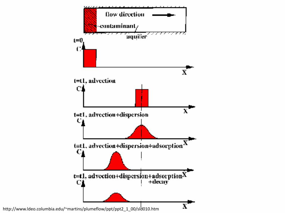
http://www.ldeo.columbia.edu/~martins/plumeflow/ppt/ppt2_1_00/sld010.htm

Diffusion Law

• Darcy’s law for relates fluid flux to hydraulic gradient: q = -K dh/dx

• For mass transport, there is a similar law (Fick’s law) relating solute flux to concentration gradient in a pure liquid: J = -Dd. dC/dx

where J is the chemical mass flux [moles. L-2T-1]

C is concentration [moles.L-3]

Dd is the diffusion coefficient [L2T-1]

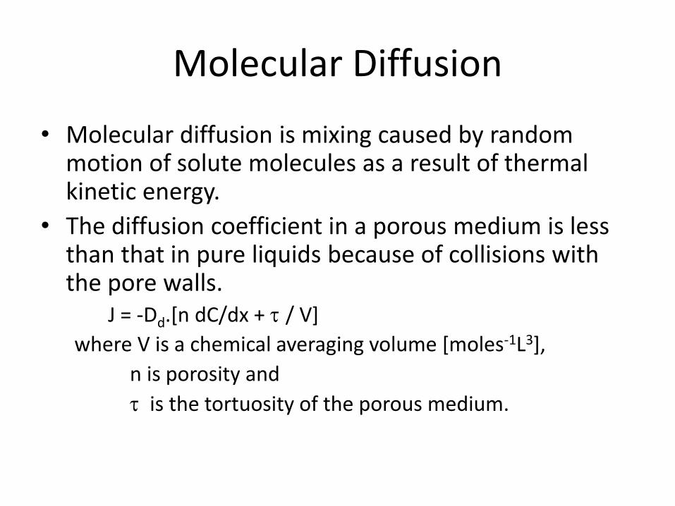
Molecular Diffusion

• Molecular diffusion is mixing caused by random motion of solute molecules as a result of thermal kinetic energy.

• The diffusion coefficient in a porous medium is less than that in pure liquids because of collisions with the pore walls. J = -Dd.[n dC/dx + t / V]

where V is a chemical averaging volume [moles-1L3],

n is porosity and

t is the tortuosity of the porous medium.

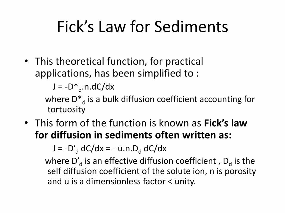
Fick’s Law for Sediments

• This theoretical function, for practical applications, has been simplified to : J = -D*d.n.dC/dx

where D*d is a bulk diffusion coefficient accounting for tortuosity

• This form of the function is known as Fick’s law for diffusion in sediments often written as: J = -D’d dC/dx = - u.n.Dd dC/dx

where D’d is an effective diffusion coefficient , Dd is the self diffusion coefficient of the solute ion, n is porosity and u is a dimensionless factor < unity.

Estimating D’d

• The factor u depends on the tortuosity of the medium and empirical values (Hellferich, 1966) lie between 0.25 and 0.50

• Bear (1972) suggest values between 0.56 and 0.80 based on a theoretical evaluation of granular media.

• Whatever the factor used, D’d increases with increasing porosity and decreases with increasing tortuosity t = Le/L

Dd for Common Ions Cation Dd (10-10 m2/s) Anion Dd (10-10 m2/s)

H+ 93.1 OH- 52.7

K+ 19.6 Cl- 20.3

Na+ 13.3 HS- 17.3

HCO3- 11.8

Ca2+ 7.93 SO42- 10.7

Fe2+ 7.19 CO32- 9.55

Mg2+ 7.05

Fe3+ 6.07

Typical factors to calculate D’d are 0.10 to 0.20 for granular materials

Notice that diffusion coefficients are smaller the higher the charge on the ion

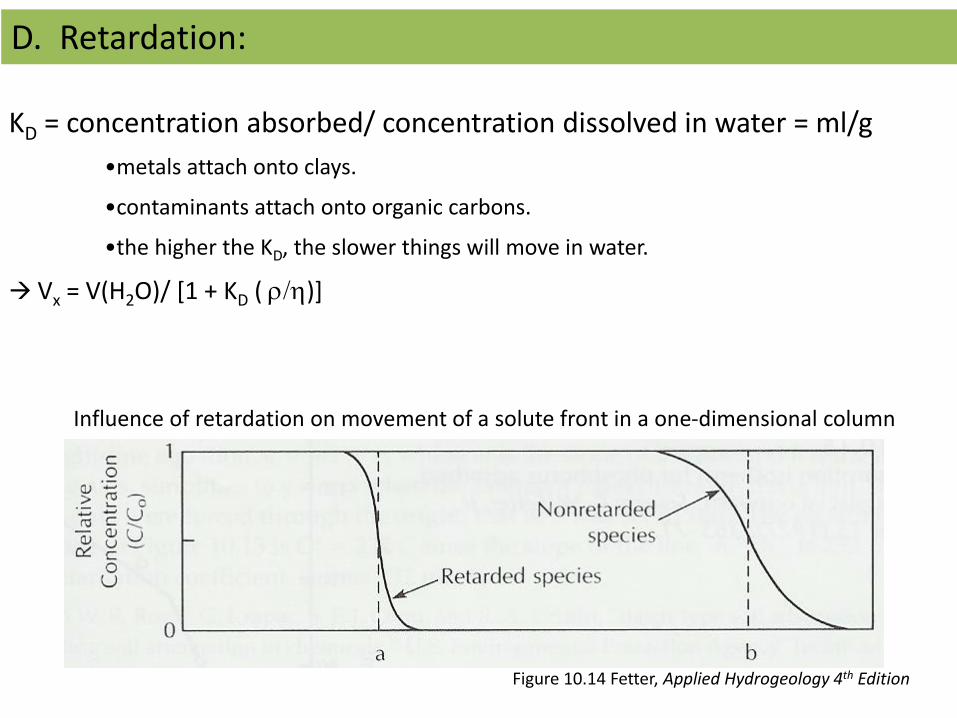
KD = concentration absorbed/ concentration dissolved in water = ml/g

•metals attach onto clays.

•contaminants attach onto organic carbons.

•the higher the KD, the slower things will move in water.

Vx = V(H2O)/ [1 + KD ( r/h)]

Influence of retardation on movement of a solute front in a one-dimensional column


D. Retardation:

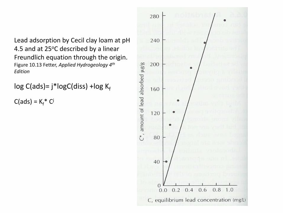
Lead adsorption by Cecil clay loam at pH 4.5 and at 25oC described by a linear Freundlich equation through the origin. Figure 10.13 Fetter, Applied Hydrogeology 4th Edition

log C(ads)= j*logC(diss) +log Kf

C(ads) = Kf* Cj

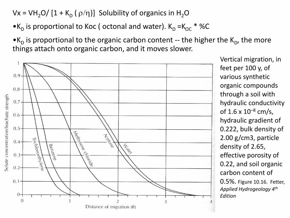
Vx = VH2O/ [1 + KD ( r/h)] Solubility of organics in H2O

•KD is proportional to Koc ( octonal and water). KD =KOC * %C

•KD is proportional to the organic carbon content -- the higher the KD, the more things attach onto organic carbon, and it moves slower.

Vertical migration, in feet per 100 y, of various synthetic organic compounds through a soil with hydraulic conductivity of 1.6 x 10–8 cm/s, hydraulic gradient of 0.222, bulk density of 2.00 g/cm3, particle density of 2.65, effective porosity of 0.22, and soil organic carbon content of 0.5%. Figure 10.16. Fetter,

Applied Hydrogeology 4th Edition

Solubilities and Octanol-Water Partition Coefficients for Some Common Organic Pollutants Table 6-5. Drever The Geochemistry of Natural Waters 3rd Edition

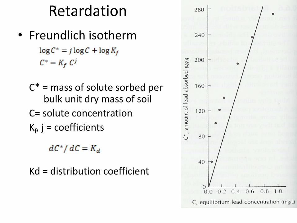
Retardation

• Freundlich isotherm

C* = mass of solute sorbed per

bulk unit dry mass of soil

C= solute concentration

Kf, j = coefficients

Kd = distribution coefficient

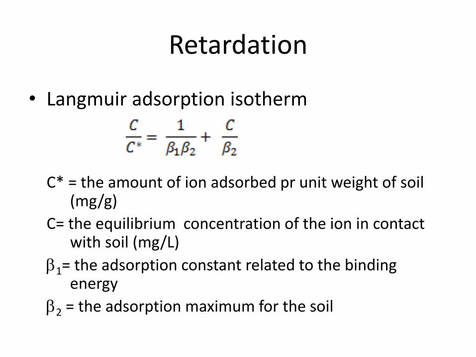
Retardation

• Langmuir adsorption isotherm

C* = the amount of ion adsorbed pr unit weight of soil

(mg/g)

C= the equilibrium concentration of the ion in contact with soil (mg/L)

b1= the adsorption constant related to the binding energy

b2 = the adsorption maximum for the soil

• Retardation factor (R)

rb = dry bulk mass density q= volumetric moisture content of soil Kd = distribution coefficient for the solute with the soil Vx = average linear velocity Vc = velocity of the solute front

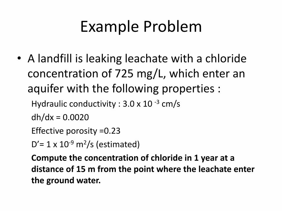
Example Problem

• A landfill is leaking leachate with a chloride concentration of 725 mg/L, which enter an aquifer with the following properties : Hydraulic conductivity : 3.0 x 10 -3 cm/s

dh/dx = 0.0020

Effective porosity =0.23

D’= 1 x 10-9 m2/s (estimated)

Compute the concentration of chloride in 1 year at a distance of 15 m from the point where the leachate enter the ground water.

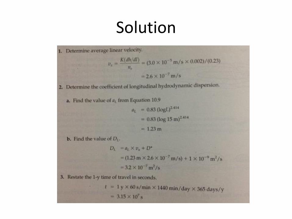
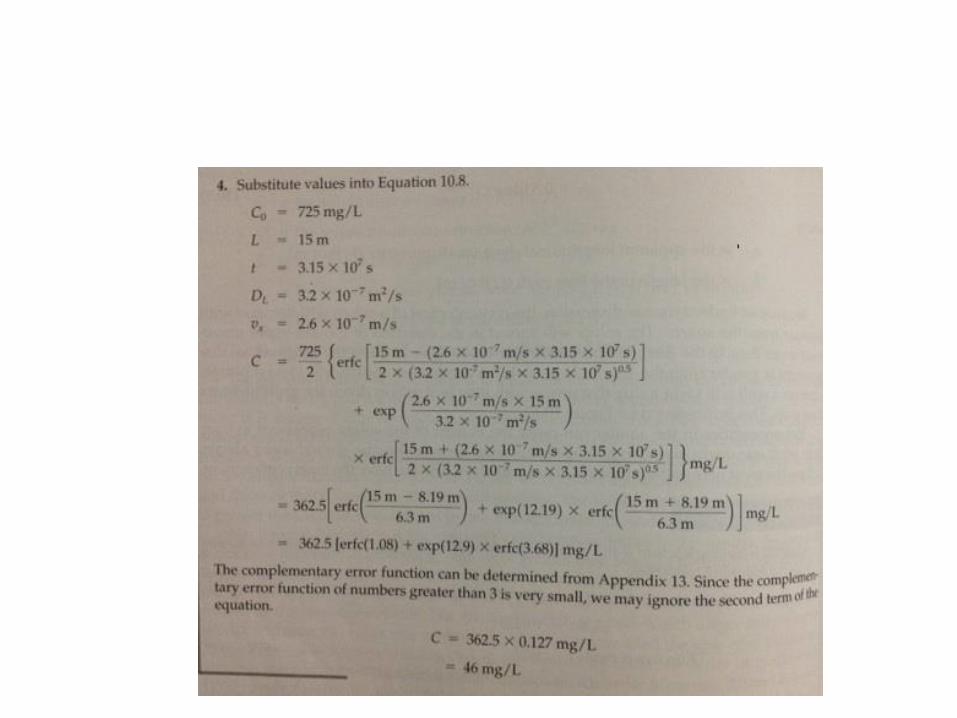
Solution

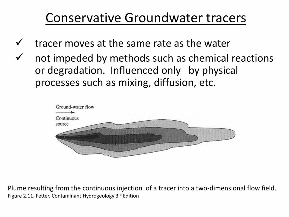
Conservative Groundwater tracers

tracer moves at the same rate as the water

not impeded by methods such as chemical reactions or degradation. Influenced only by physical processes such as mixing, diffusion, etc.

Plume resulting from the continuous injection of a tracer into a two-dimensional flow field. Figure 2.11. Fetter, Contaminant Hydrogeology 3rd Edition

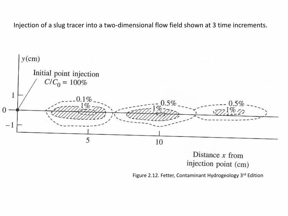
Injection of a slug tracer into a two-dimensional flow field shown at 3 time increments.


Experimental Continuous Tracer

Time

C/C

o

0

1

Start

Time

C/C

o

0

1

Start

INFLOW A OUTFLOW B

A B

Continuous Tracer Test

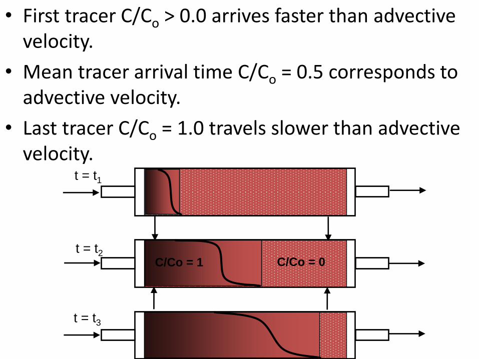
• First tracer C/Co > 0.0 arrives faster than advective velocity.

• Mean tracer arrival time C/Co = 0.5 corresponds to advective velocity.

• Last tracer C/Co = 1.0 travels slower than advective velocity.

t = t1

t = t2

t = t3

C/Co = 0 C/Co = 1

• First tracer C/Co > 0.0 arrives faster than advective velocity.

• Mean tracer arrival time C/Co = 0.5 corresponds to advective velocity.

• Last tracer C/Co = 1.0 travels slower than advective velocity.

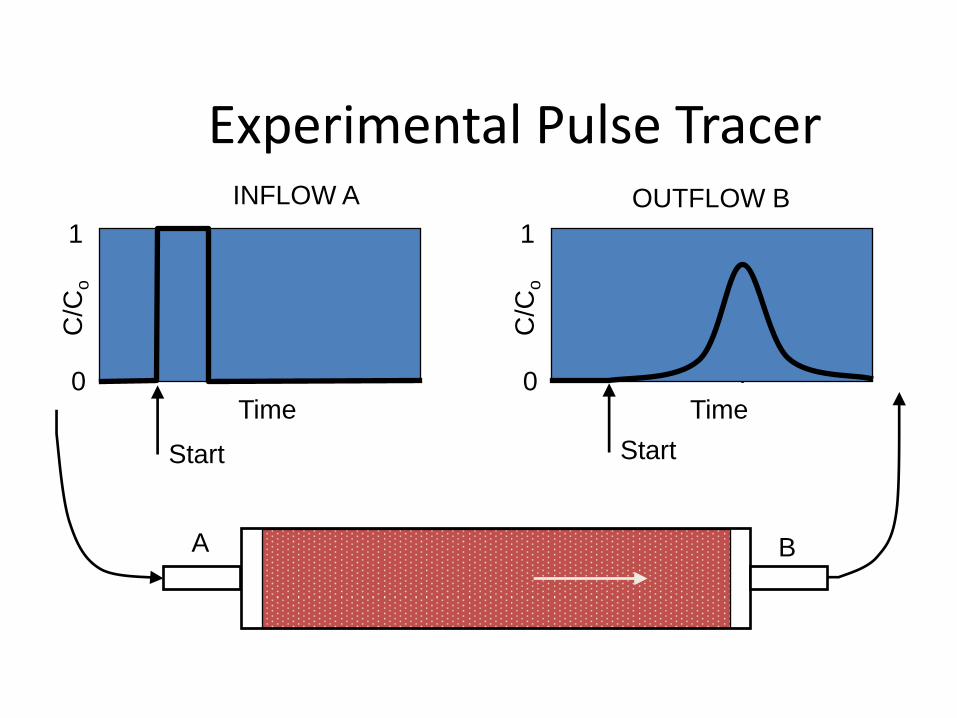
Experimental Pulse Tracer

Time

C/C

o

0

1

Start

Time

C/C

o

0

1

Start

INFLOW A OUTFLOW B

A B

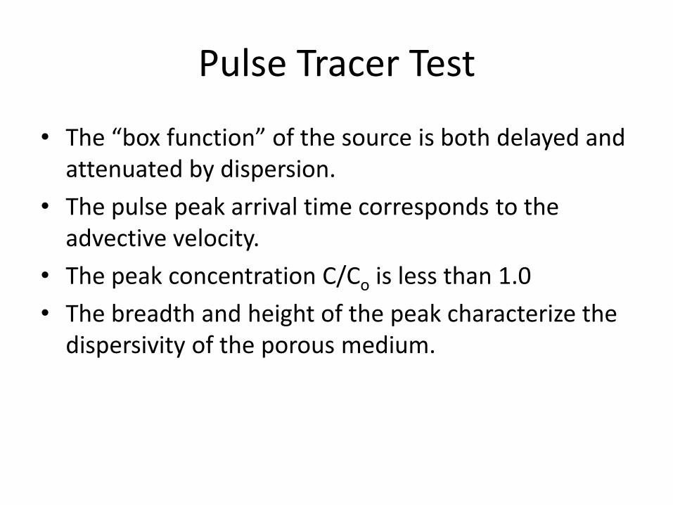
Pulse Tracer Test

• The “box function” of the source is both delayed and attenuated by dispersion.

• The pulse peak arrival time corresponds to the advective velocity.

• The peak concentration C/Co is less than 1.0

• The breadth and height of the peak characterize the dispersivity of the porous medium.

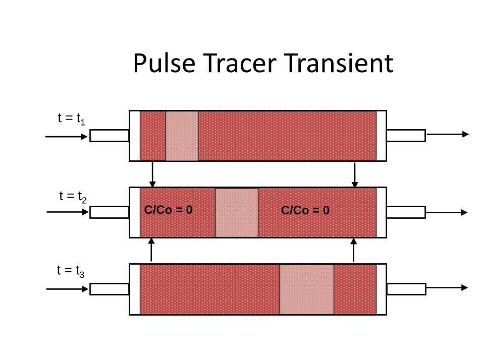
Pulse Tracer Transient

t = t1

t = t2

t = t3

C/Co = 0 C/Co = 0

Pulse Zone of Dispersion

• The zone of dispersion broadens and the peak concentration C/Co reduces as it moves through the porous medium.

• Ahead of the zone C/Co = 0

• Behind the zone C/Co =0

slide -5 solute transport - institut teknologi bandung · tl 3106 pencemaran tanah (soil...

Documents