slide 18.1 time structured data mathematicalmarketing chapter 18 econometrics this series of slides...
Post on 19-Dec-2015
215 views
TRANSCRIPT

Slide 18.Slide 18.11Time Structured DataTime Structured Data
MathematicalMathematicalMarketingMarketing
Chapter 18 Econometrics
This series of slides will cover a subset of Chapter 18
Data and Operators
Autocorrelated
Lagged Variables
Partial Adjustment

Slide 18.Slide 18.22Time Structured DataTime Structured Data
MathematicalMathematicalMarketingMarketing
Repeated Firm or Consumer Data
Time Structured Data - [y1, y2, …, yt, …, yT]
Error Structure - Not Gauss-Markov (2I)

Slide 18.Slide 18.33Time Structured DataTime Structured Data
MathematicalMathematicalMarketingMarketing
Backshift Operator
The backshift operator, B, by definition produces xt-1 from xt
Bxt = xt-1
Of course, one can also say
BBxt = B2xt = xt-2
In general,
Bjxt = xt-j
Slide 18.Slide 18.44Time Structured DataTime Structured Data
MathematicalMathematicalMarketingMarketing
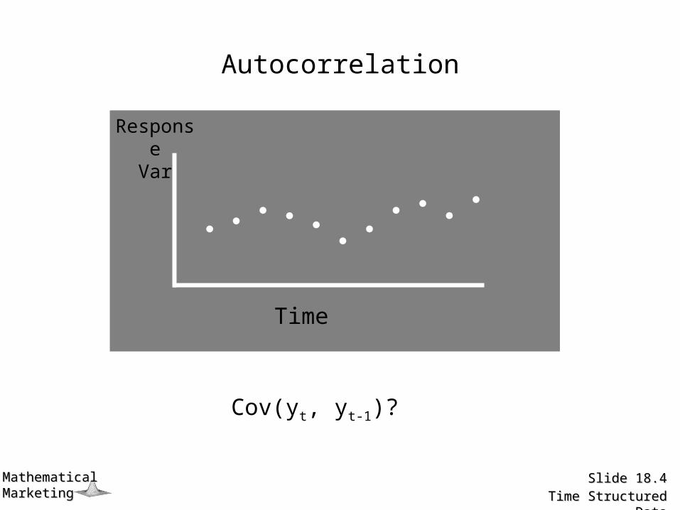
Autocorrelation
Time
ResponseVar
Cov(yt, yt-1)?
Slide 18.Slide 18.55Time Structured DataTime Structured Data
MathematicalMathematicalMarketingMarketing
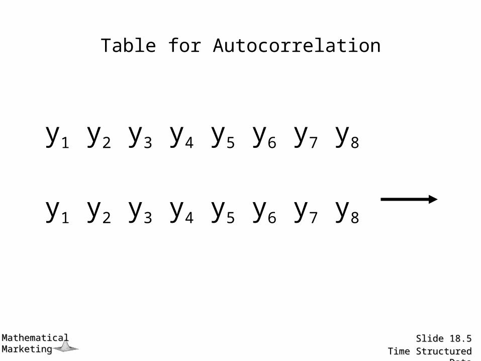
Table for Autocorrelation
y1 y2 y3 y4 y5 y6 y7 y8
y1 y2 y3 y4 y5 y6 y7 y8

Slide 18.Slide 18.66Time Structured DataTime Structured Data
MathematicalMathematicalMarketingMarketing
Table for Autocorrelation
y1 y2 y3 y4 y5 y6 y7 y8
y1 y2 y3 y4 y5 y6 y7 y8
Slide 18.Slide 18.77Time Structured DataTime Structured Data
MathematicalMathematicalMarketingMarketing
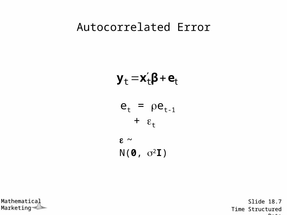
Autocorrelated Error
ttt eβxy
et = et-1 + t
~ N(0,2I)

Slide 18.Slide 18.88Time Structured DataTime Structured Data
MathematicalMathematicalMarketingMarketing
Recursive Substitution in Time Series
et = et-1 + t
= (et-2 + t-1) + t
= [(et-3 + t-2) + t-1] + t
Slide 18.Slide 18.99Time Structured DataTime Structured Data
MathematicalMathematicalMarketingMarketing
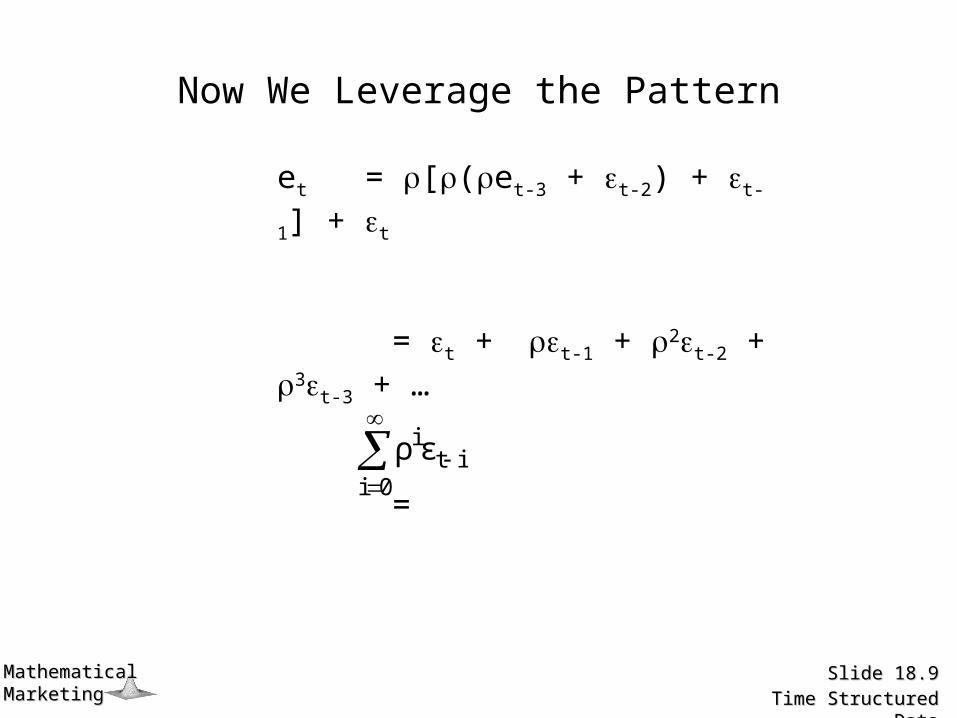
Now We Leverage the Pattern
et = [(et-3 + t-2) + t-1] + t
= t + t-1 + 2t-2 + 3t-3 + …
=
0iit
iερ

Slide 18.Slide 18.1010Time Structured DataTime Structured Data
MathematicalMathematicalMarketingMarketing
Time to Figure Out E(·)
0)E(ερ
ερE)E(e
0iit
i
0iit
it

Slide 18.Slide 18.1111Time Structured DataTime Structured Data
MathematicalMathematicalMarketingMarketing
And Now Of course V(·)
V(et) = E[et - E(et)]2
The previous slide showed that E(et) = 0
V(et) = E[et2]
Slide 18.Slide 18.1212Time Structured DataTime Structured Data
MathematicalMathematicalMarketingMarketing
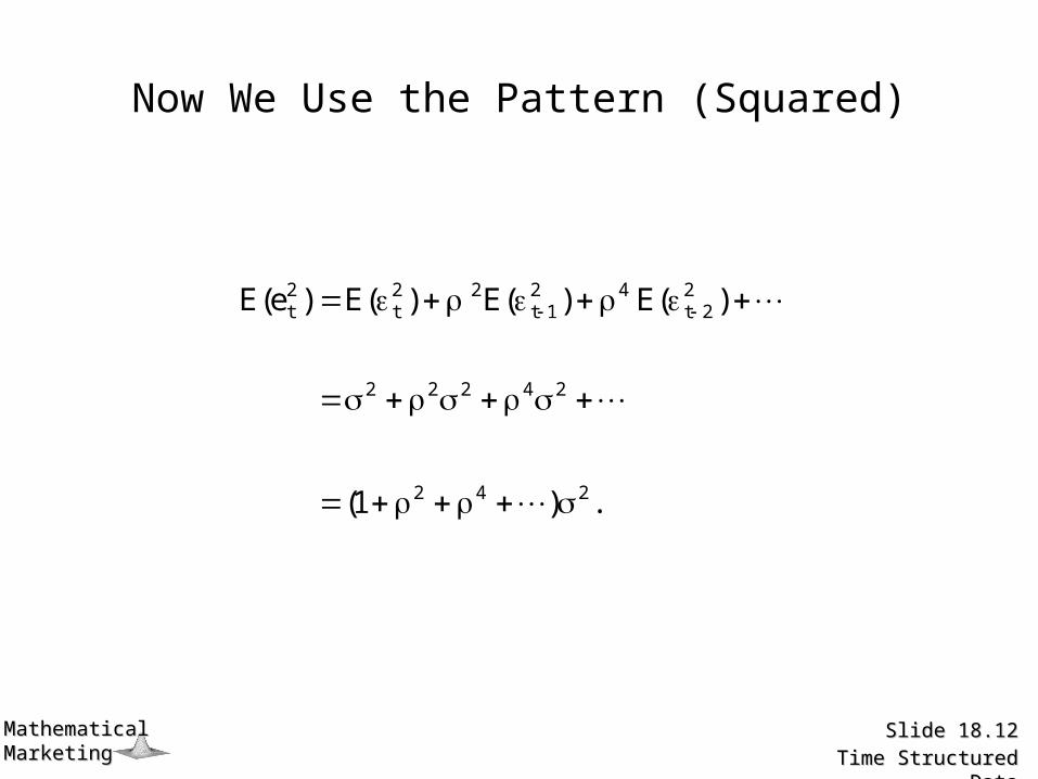
Now We Use the Pattern (Squared)
.)1(
)(E)(E)(E)e(E
242
24222
22t
421t
22t
2t

Slide 18.Slide 18.1313Time Structured DataTime Structured Data
MathematicalMathematicalMarketingMarketing
A Big Mess, Right?
V(et) = E(et2) = (1 + 2 + 4 + …)2
Uh-oh… an infinite series…

Slide 18.Slide 18.1414Time Structured DataTime Structured Data
MathematicalMathematicalMarketingMarketing
Let’s Define the Infinite Series “s”
s = 1 + 2 + 4 + 8 + …
2s = 2 + 4 + 8 + 16 + …
What is the difference between the first and second lines?
s - 2s = 1
.1
1s
2

Slide 18.Slide 18.1515Time Structured DataTime Structured Data
MathematicalMathematicalMarketingMarketing
Putting It Together
.1
1s
2
2
222
e2t ρ1
σsσσ)E(e
Since

Slide 18.Slide 18.1616Time Structured DataTime Structured Data
MathematicalMathematicalMarketingMarketing
Applying the Same Logic to the Covariances
2e1tt ρσ)e,E(e
2e
jjtt σρ)e,Cov(e
For any pair of errors one time unit apart we have
and in general

Slide 18.Slide 18.1717Time Structured DataTime Structured Data
MathematicalMathematicalMarketingMarketing
Instead of the Gauss-Markov Assumption (2I) we have
VV2
22e
ρ1
σσ
1ρρρ
ρ1ρρ
ρρ1ρ
ρρρ1
3n2n1n
3n2
2n
1n2
V
V(e) =
So how do we estimate now?

Slide 18.Slide 18.1818Time Structured DataTime Structured Data
MathematicalMathematicalMarketingMarketing
Lagged Independent Variables
yt = 0 + xt-11 + et
Consumer behavior and attitude do not immediately change:
yt = 0 + xt-11 + xt-22 + ··· + et
Or more generally:

Slide 18.Slide 18.1919Time Structured DataTime Structured Data
MathematicalMathematicalMarketingMarketing
Koyck’s Scheme
Koyck started with the infinite sequence
yt = xt0 + xt-11 + xt-22 + ··· + et
and assumed that the values are all of the same sign
.c0i
i

Slide 18.Slide 18.2020Time Structured DataTime Structured Data
MathematicalMathematicalMarketingMarketing
Lagged effects can take on many forms:
i
i
0 s
i
i
0 s
i
i
0 s
Koyck (and others) have come up with ways of estimating different shaped impacts (1) assuming that only s lag positions really matter, and that (2) the
impact of x on y takes on some sort of curved pattern as above

Slide 18.Slide 18.2121Time Structured DataTime Structured Data
MathematicalMathematicalMarketingMarketing
Further Assumptions
1. How many lags matter? In other words, how far back do we really need to go? Call that s.
2. Can we express the impact of those s lags with an even fewer number of unknowns. Any pattern can be approximated with a polynomial of degree r s (Almon’s Scheme). In Koyck’s Scheme, we will use a geometric rather than polynomial pattern.

Slide 18.Slide 18.2222Time Structured DataTime Structured Data
MathematicalMathematicalMarketingMarketing
We Rewrite the Model Slightly
t2t21t1t0
t22t11t0tt
e]xwxwxw[
exxxy
where wi 0 for i = 0, 1, 2, ···, and
0i
i 1w

Slide 18.Slide 18.2323Time Structured DataTime Structured Data
MathematicalMathematicalMarketingMarketing
Bring in the Backshift Operator and Assume a Geometric Pattern for the wi
.ex]BwBww[ tt2
210
t2t21t1t0t e]xwxwxβ[wy
Now we assume that
wi = (1 - )i
0 < < 1

Slide 18.Slide 18.2424Time Structured DataTime Structured Data
MathematicalMathematicalMarketingMarketing
Given Those Assumptions
λB1
1λ)(1
)BλλBλ)(1(1BwBww 222
210
Anyone care to say how we got to this fraction?

Slide 18.Slide 18.2525Time Structured DataTime Structured Data
MathematicalMathematicalMarketingMarketing
Substitute That into the Equation for yt
)ee(yx)1(y
Bee)x-(1Byy
e)B1()x-(1y)B1(
exB1
)1(y
1tt1ttt
ttttt
ttt
ttt

Slide 18.Slide 18.2626Time Structured DataTime Structured Data
MathematicalMathematicalMarketingMarketing
Adaptive Adjustment
Define
as the expected level of x (prices, availability, quality, outcome)… So consumer
behavior should look like
.ex~y t1t0t
tx~

Slide 18.Slide 18.2727Time Structured DataTime Structured Data
MathematicalMathematicalMarketingMarketing
Updating Process
.xx~)1(x~
x~)1(x
x~x~xx~
)x~x(x~x~
t1tt
1tt
1t1ttt
1tt1tt
Expectations are updated by a fraction of the discrepancy between the current observation and the previous expectation

Slide 18.Slide 18.2828Time Structured DataTime Structured Data
MathematicalMathematicalMarketingMarketing
Redefine in Terms of a New Parameter
Define
= 1 -
so that
t1tt δxx~λx~
t1tt δxx~δ)(1x~

Slide 18.Slide 18.2929Time Structured DataTime Structured Data
MathematicalMathematicalMarketingMarketing
More Algebra
.xB1
x~
xx~)B1(
xx~x~
tt
tt
t1tt

Slide 18.Slide 18.3030Time Structured DataTime Structured Data
MathematicalMathematicalMarketingMarketing
Back to the Model for yt
We end up at the same place as slide 25
tt1
0
tt1
0
t1t0t
exλB1
λ)(1ββ
exλB1
δββ
eβx~βy