1

Slicing up Global Value Chains:

The Role of China

Abdul Azeez Erumbana

Bart Losa

Robert Stehrerb

Marcel Timmer a,*

Gaaitzen de Vriesa

Version February 28, 2011

NB The results in this paper are preliminary and should not be quoted

Affiliations a Groningen Growth and Development Centre, University of Groningen b The Vienna Institute for International Economic Studies (wiiw)

* Corresponding Author

Marcel P. Timmer

Groningen Growth and Development Centre

Faculty of Economics and Business

University of Groningen, The Netherlands

m.p.timmer@rug.nl

2

Abstract

In this paper we provide a new metric for the contributions of countries to global value

chains. It is based on an input-output analysis of vertically integrated industries, taking

into account trade in intermediate inputs within and across countries. The value of global

manufacturing output is allocated to labour and capital employed in various regions in the

world. Using a new world input-output database, we find that an increasing part of the

output value in Chinese manufacturing is captured as income by production factors

outside China, up to 32 per cent in electrical machinery in 2006. The value captured by

China in foreign production appeared to be smaller, but also increasing over time. We

also find that the growth of Chinese manufacturing has led to major changes in the

income of production factors around the world. Overall labour income related to global

manufacturing in the EU and NAFTA changed only marginally, even for low- and

medium-skilled workers. In contrast, incomes in Japan declined for all production factors,

in particular medium-skilled labour and capital.

Acknowledgements:

This paper is part of the World Input-Output Database (WIOD) project funded by the

European Commission, Research Directorate General as part of the 7th Framework

Programme, Theme 8: Socio-Economic Sciences and Humanities, grant Agreement no:

225 281. More information on the WIOD-project can be found at www.wiod.org.

3

1. Introduction

Since the 1960s the global economy is rapidly integrating through spectacular increases

in international trade in goods and services. Initially this process mainly involved

integration within Europe, and in the triad of Europe, the US and Japan. This was

followed by the rise of East-Asia and later the other newly industrialising countries in

Asia, led by Japan in a pattern of development known as the flying geese. More recently,

India and in particular China started to take part in this process as well. The increasing

integration of world markets was accompanied by a fragmentation of production

processes as activities once done in the home economy were increasingly off shored.

Fostered by rapidly falling communication, coordination and transport costs, the various

stages of manufacturing needed not be performed near to each other. For example,

whereas in the past the production of personal computers took mainly place within the

U.S., now the separate phases of design, component production, assembly, testing and

packaging are scattered around the world. This great unbundling of tasks, also known as

fragmentation, off shoring or vertical specialisation, has deep implications for the

organisation and coordination of activities around the globe. Through the trade of

intermediate goods and services, global production networks developed quickly in

manufacturing industries such as textiles, automotive and electronics industries, and also

increasingly in various services industries. This increased competitive pressures around

the world. The rise of China has raised fears about the hollowing out of industrial activity

in Europe and the US, not only in basic low-tech manufacturing, but increasingly also in

more sophisticated industries and services. Between 1995 and 2006 the share of China in

global manufacturing exports increased from 4 % to 11%. Its share in manufacturing of

electrical equipment (ISIC industries 30-33) increased even more dramatically from 4%

to 22%.1 These statistics are often taken as prima facie evidence of the increasing

sophistication of Chinese production and associated competitive threats to the rest of the

world.

However, export statistics can be misleading as the value of exports of a country conveys

little information on the value actually added in the exporting country. The latter is much

more relevant for any assessment of where value is created and captured in today’s global

production networks. For example, Dedrick et al. (2010) show that for a number of

electronic products (iPods and laptops) that are manufactured in China, less than 3 per

cent of the export value is actually captured by the Chinese activities. The major part of

the value is captured by firms in the US, Japan, Korea and Taiwan through delivery of

sophisticated intermediate inputs. The value added by China in production of these high-

tech goods is rather limited, and mainly consists of low-skilled assembly services. Such

analyses clearly bring out the limitations of export statistics as an indicator for

1 Source: World Input-Output database, see Table 1.

4

competitiveness. But so far we do not know to what extent these product case studies are

representative for overall Chinese exports, and they convey little information on possible

trends in the share of the global value aded captured by China. This is the main

motivation for the analysis in this paper.

In this paper we introduce a new metric that allows us to analyse the value that is added

in various stages of regionally dispersed production processes. It is based on a new

industry-level database that combines national input-output tables, bilateral international

trade statistics and production factor requirements. A crucial characteristic of this metric

is the explicit recognition of national and international trade in intermediate products. It is

the first attempt to quantify and track the process known as the slicing of global value

chains (Krugman, 1995). The value chain of output is sliced into income for labour and capital

in various regions in the world. In this approach, a country can increase its income domestically

through increased value of local production of final goods and an increased share of domestic

value added in this value, or by capturing a larger share of foreign value chains. Our global

value chain (GVC) metric will not only show in which countries value is being added, but

also by which type of production factor such as low- and high-skilled labour or capital.

One of the main concerns of the global fragmentation process is the uneven effects on

remuneration of various groups of labourers and capital owners, both within and across

countries. The GVC metric will indicate possible trends in where profits are reaped and to

whom wages are paid. In this paper we will focus in particular on the increasing

prominence of China in various manufacturing value chains, and identify how this has

impacted wages and profits in other countries. Our aim is to establish a series of stylised

facts that can serve as a starting point for deeper analysis of the causes of these global

shifts.

Our approach is closely related to the work on measures of vertical specialisation. The

seminal work of Hummels et al. (2001) has spurned various attempts to measure the

factor content of trade flows such as Reimer (2006), Johnson (2008) and Trefler and Zhu

(2010). Other authors aim to measure the factor content of trade for specific countries

such as Feenstra and Hong (2010) for China.2 We follow this literature by acknowledging

the important role of international trade in intermediate products. But rather than

focussing on the factor content of trade of individual countries we analyse vertically

integrated value chains. In addition, detailed data on production factors allows us to

analyse trends in income of labour and capital inputs, and not only overall value added.

This allows for a sharper focus on the impact of for example changes in factor

endowments on the shares countries capture in the global value chains.

Our GVC metrics also provide additional quantitative evidence for the trends in

global production networks that have been analysed in more qualitative terms by for

2 See also de Backer and Yamano (2007). Foster and Stehrer (2010) provide a recent overview.

5

example Kaplinsky (2000), Gereffi (1999) and Sturgeon, van Biesebroeck and Gereffi

(2008). These studies focus on the development of global production networks in

particular industries such as textiles and automobiles, and analyse how these increasingly

complex systems are governed and coordinated.

The rest of the paper is organised as follows. In Section 2 we introduce our new GVC

metric by means of an iPod value chain example. We then present our mathematical

approach that is based on Leontief’s decomposition technique well known from input-

output analysis. In Section 3, the construction of the new WIOD database is discussed

and data sources described, including those for China. Results of the GVC

decompositions for detailed manufacturing industries are discussed in Section 4. Section

5 concludes.

2. Quantifying global value chains (GVCs)

In this section we introduce our new GVC metric. We start with an example of a product

GVC to illustrate the various concepts involved, based on the case study of Apple’s iPod

by Linden at al. (2010). This example shows the existence of intricate regional production

networks feeding into each other, underlining the importance of distinguishing direct and

indirect contributions to production. In section 2.2 we outline our proposal for

generalising this approach and introduce a GVC metric for broad product categories such

as wearing apparel or electronics. It is based on the measurement of embodied (direct and

indirect) production factor services from various countries in the value of a set of final

goods through the use of a world input-output table.

2.1 Global value chain of an iPod

Linden et al. (2009) and Dedrick et al. (2010) provide a detailed analysis of the various

activities in the production of the so-called Video iPod, the 30GB version of Apple’s fifth

generation iPods. Their case study shows the strong global fragmentation of the

production process of high-end electronic products. The lead firm in this production chain

is Apple, a US multinational company, that has designed the iPod and organises its

production. The iPod is manufactured in mainland China through assembling of several

hundreds of components and parts. Based on professional industry sources, Linden et al.

traced the origins and values of the various components and found that most of them, in

particular the more expensive ones did not originate from China, but from Japan, the US,

Korea, Taiwan and other Asian countries. In addition, some of these components, such as

the Japanese hard-disc drives are themselves the end-product of a global production chain

as they are assembled out of more elementary components manufactured elsewhere.

6

In Figure 1, a highly stylised representation of the main stages of the global

production network of the iPod is provided. The figure shows how components are

imported into China to be assembled into the iPod, which is subsequently exported to the

warehouses of the lead firm Apple in the US, before being sold to final customers

throughout the world through various distribution and retail channels. The main

components of the iPod are the hard disc drive (HDD) and display from Japan, processors

from the US and the battery from South Korea, alongside hundreds of other small

components. For the production process also various business services inputs are needed,

as well as energy. We also indicated the production chain of the hard disc drive (HDD)

which is the major component of the iPod. This chain is led by Toshiba, a Japanese firm,

but assembly takes place in China and the Philippines, based on components sourced

from around the world. The production of the other components for the iPod have not

been detailed any further.

[Fig 1 about here]

Within the iPod production chain, each participant purchases inputs and then adds value

which becomes part of the cost for the next stage of production. The sum of the value

added by all participants in the chain equals the final product price paid by the customer.

This is indicated in two rows below the figure which indicate the price at a particular

point in the production chain and the value added at a particular production stage (based

on Table A2 from Dedrick et al. 2010 and Table 1 from Linden et al. 2009). The final

consumer price of the iPod in the US is 299$. Of this, about 75$ is added by distribution

and retailing services. In this case of US customers, this value is provided by mainly US

wholesalers and retailers, but this value could also be captured by other countries in case

the iPod is sold in other markets. Apple, a US company, is estimated to capture about 80$

of each iPod.3 In this paper we do not analyse the margins generated after the production

of the final good, and focus instead on the distribution of the good’s value as represented

by its ex-factory value.

The ex-factory price of the iPod when shipped from China is about 144$. The

value added in China through assembling is rather limited and estimated at around 4$

only. The remainder of about 140$ represents cost to the Chinese assembler as high-value

components have to be sourced from elsewhere such as the Japanese HDD making up

about half of the factory iPod price (73$), the display (23$), the processors (13$), the

battery (3$) and the rest (29$). Linden et al. (2010) also show for some other high-end

electronic products such as notebooks that the assembling done by Chinese factories

captures at most 3 per cent of the ex factory price

3 This is compensation for Apple’s provision of intangible services such as software and designs, market

knowledge, intellectual property, system integration and cost management skills and a high-value brand

name.

7

However, the contribution of China to the iPod value chain is not limited to its

iPod assembling activities, as Chinese factories are also involved in the production chains

of some of the components, in particular in the assembling of the HDD and also in the

manufacturing of some of its components. Unfortunately, Linden at al. (2009) do not

further decompose the contribution of China in these upstream activities but hypothesize

that the overall Chinese contribution to the iPod value chain will be very limited due to

the capital-intensive production process of most electronic components. In our analysis

we will try to uncover the total contribution of Chinese production factors in the various

stages of production.

The iPod example clearly illustrates the basic concept of a global value chain.

Value is added at various stages of production through the utilisation of production

factors labour and capital (including tangible capital such as machinery and land, as well

as intangible capital such as software and knowledge). Through the use of intermediate

products, value added in previous stages is embodied in the value of the final product. It

provides a clear picture of how the final product value is sliced by the various firms and

regions involved. To assess the contribution of Chinese production factors, one has to add

up the value added by Chinese factories at the various stages of production. This includes

not only the direct contribution through assembly of the final product but also the indirect

contributions through intermediate inputs. The latter can be sizeable particularly in

situations where production relies heavily on the use of imported intermediates.

The case study of the iPod might not be representative for the overall capture of China in

the GVC in electronics. More generic and mature electronic products might provide

greater opportunities for China to capture a larger part of the value. To analyse this we

introduce our new GVC metric that is based on more aggregate industry data rather than

product-level analysis.

2.2 A new GVC metric

Our aim is to decompose the value of a final product into the value added by various

production factors in various regions in the world. The approach follows the standard

approach in the input-output literature and traces the amount of factor inputs needed to

produce a certain amount of final demand (see e.g. Miller and Blair, 2009). Variations of

this approach are also used in the bourgeoning literature on trade in value added (e.g.

Reimer 2006 and Trefler and Zhu, 2010). The key element in this approach is that not

only direct, but also indirect contributions are taken into account. The value of the final

product will not only contain value added by production factors in the industry producing

the final product, but also by factors employed in other domestic and foreign industries

through the use of intermediate inputs. The size of these indirect effects depend on the

interrelatedness of production as will be represented in a world input-output table.

8

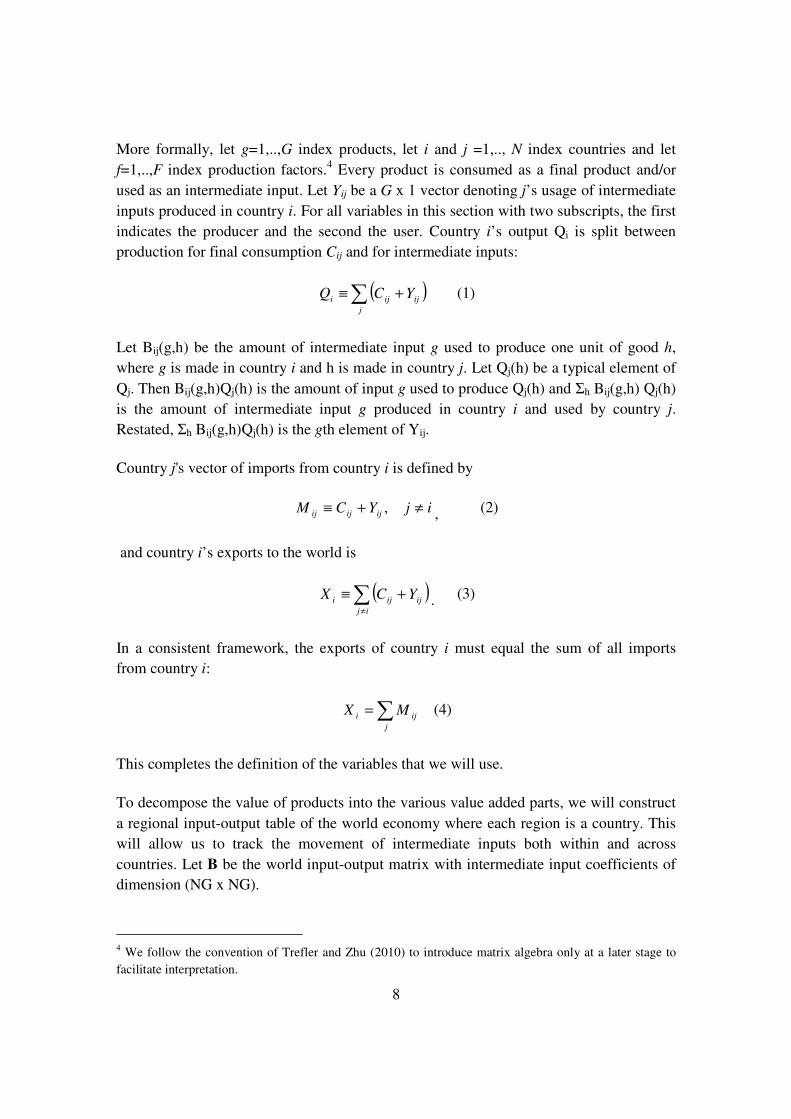
More formally, let g=1,..,G index products, let i and j =1,.., N index countries and let

f=1,..,F index production factors.4 Every product is consumed as a final product and/or

used as an intermediate input. Let Yij be a G x 1 vector denoting j’s usage of intermediate

inputs produced in country i. For all variables in this section with two subscripts, the first

indicates the producer and the second the user. Country i’s output Qi is split between

production for final consumption Cij and for intermediate inputs:

( )∑ +≡j

ijiji YCQ (1)

Let Bij(g,h) be the amount of intermediate input g used to produce one unit of good h,

where g is made in country i and h is made in country j. Let Qj(h) be a typical element of

Qj. Then Bij(g,h)Qj(h) is the amount of input g used to produce Qj(h) and Σh Bij(g,h) Qj(h)

is the amount of intermediate input g produced in country i and used by country j.

Restated, Σh Bij(g,h)Qj(h) is the gth element of Yij.

Country j's vector of imports from country i is defined by

ijYCM ijijij ≠+≡ , , (2)

and country i’s exports to the world is

( )∑≠

+≡ij

ijiji YCX . (3)

In a consistent framework, the exports of country i must equal the sum of all imports

from country i:

∑=j

iji MX (4)

This completes the definition of the variables that we will use.

To decompose the value of products into the various value added parts, we will construct

a regional input-output table of the world economy where each region is a country. This

will allow us to track the movement of intermediate inputs both within and across

countries. Let B be the world input-output matrix with intermediate input coefficients of

dimension (NG x NG).

4 We follow the convention of Trefler and Zhu (2010) to introduce matrix algebra only at a later stage to

facilitate interpretation.

9

≡

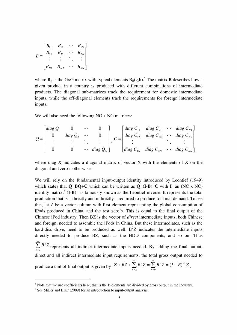
NNNN

N

N

BBB

BBB

BBB

B

L

MOMM

L

L

21

22221

11211

where Bij is the GxG matrix with typical elements Bij(g,h).5 The matrix B describes how a

given product in a country is produced with different combinations of intermediate

products. The diagonal sub-matrices track the requirement for domestic intermediate

inputs, while the off-diagonal elements track the requirements for foreign intermediate

inputs.

We will also need the following NG x NG matrices:

≡

NQdiag

Qdiag

Qdiag

Q

L

MOMM

L

L

00

00

00

2

1

,

≡

NNNN

N

N

CdiagCdiagCdiag

CdiagCdiagCdiag

CdiagCdiagCdiag

C

L

MOMM

L

L

21

22212

12111

where diag X indicates a diagonal matrix of vector X with the elements of X on the

diagonal and zero’s otherwise.

We will rely on the fundamental input-output identity introduced by Leontief (1949)

which states that Q=BQ+C which can be written as Q=(I-B)-1C with I an (NC x NC)

identity matrix.6 (I-B)-1 is famously known as the Leontief inverse. It represents the total

production that is – directly and indirectly – required to produce for final demand. To see

this, let Z be a vector column with first element representing the global consumption of

iPods produced in China, and the rest zero’s. This is equal to the final output of the

Chinese iPod industry. Then BZ is the vector of direct intermediate inputs, both Chinese

and foreign, needed to assemble the iPods in China. But these intermediates, such as the

hard-disc drive, need to be produced as well. B2Z indicates the intermediate inputs

directly needed to produce BZ, such as the HDD components, and so on. Thus

∑∞

=2n

n ZB represents all indirect intermediate inputs needed. By adding the final output,

direct and all indirect intermediate input requirements, the total gross output needed to

produce a unit of final output is given by ZBIZBZBBZZn

n

n

n 1

02

)( −∞

=

∞

=

−==++ ∑∑ .

5 Note that we use coefficients here, that is the B-elements are divided by gross output in the industry. 6 See Miller and Blair (2009) for an introduction to input-output analysis.

10

Using this identity, we can derive production factor requirements for any vector Z. We

define matrix F as the direct factor inputs per unit of gross output with dimension FN x

NG. This matrix considers country- and industry-specific direct factor inputs. An element

in this matrix indicates the share in the value of gross output of a production factor used

directly by the country to produce a given product, for example the value of low-skilled

labour used in the Chinese electronics industry to produce one dollar of output. The

elements in F are direct factor inputs in the industry, because they do not account for

production factors embodied in intermediate inputs used by this industry. For this we

need to define a matrix A (FN x NG) as follows:

1)( −−= BIFA (5)

where A is the matrix of factor inputs required per unit of final demand. Note that A

includes both direct and indirect factor inputs, and contains coefficients. The amounts of

factor inputs that can be attributed to observed levels of final demand can then be found

by using the expression

ACK = (6)

in which K is the (FN x NG) matrix of amounts of factor inputs attributed to each of the

NG final demand levels. Each column of K provides the domestic and foreign factor

inputs needed for the production of final output of a particular good g in country j. A

typical element in K indicates the amount of a production factor f from country i,

embodied in final output of g in country j. By the logic of Leontief’s insight, the sum of

all elements in a column will be equal to the final output of this product. Thus we have

completed our decomposition of the value of final output into the value added by various

production factors around the world.

For various applications we are also interested in amounts of factors associated

with specific subgroups of final demand, such as final demand for world electronics, final

demand for Dutch products or final domestic demand in Germany. In these cases we

modify C by setting all values to zero, except for the final demand flows of interest.

3. Data construction

To implement the new GVC metric empirically, one needs data on bilateral trade flows at

the industry level. This type of information however is not systematically collected

through surveys. Instead researchers have to rely on datasets constructed outside the

official statistical systems. Various alternative datasets have been built in the past of

which the GTAP database is the most widely known and used (Narayanan and Walmsley,

2008). Other datasets are provided by the OECD (Yamano and Ahmad 2006) and IDE-

JETRO (2006). However, all these databases provide only one or a limited number of

11

benchmark year input-output tables which preclude an analysis of developments over

time. And although they provide separate import matrices, there is no detailed break-

down of imports by trade partner. For this paper we use a new database called the World

Input-Output Database (WIOD) that aims to fill this gap. The WIOD provides a time-

series of world input-output tables from 1995 onwards, dinstinguishing between 35

industries and 59 product groups. Using a novel approach national input-output tables of

forty major countries in the world are linked through international trade statistics,

covering more than 85 per cent of world GDP. The construction of the world input-output

tables will be discussed in section 3.1.

Another crucial element for this type of analysis are detailed value-added

accounts that provide information on the use of various types of labour (distinguished by

educational attainment level) and capital in production, both in quantities and values.

While this type of data is available for most OECD countries (O’Mahony and Timmer,

2009), it is not for most developing countries. In Section 3.2 we describe our data

strategy, with a particular emphasis for the Chinese data that is most important for the

topic of this paper, but at the same time the most challenging.

3.1 World Input-Output Tables (WIOTs): concepts and construction

In this section we outline the basic concepts and construction of our world input-

output tables. Basically, a world input-output table (WIOT) is a combination of national

input-output tables in which the use of products is broken down according to their origin.

Each product is produced either by a domestic industry or by a foreign industry. In

contrast to the national input-output tables, this information is made explicit in the WIOT.

For each country, flows of products both for intermediate and final use are split into

domestically produced or imported. In addition, the WIOT shows for imports in which

foreign industry the product was produced. This is illustrated by the schematic outline for

a WIOT in Figure 2. It illustrates the simple case of three regions: countries A and B, and

the rest of the world. In WIOD we will distinguish 40 countries and the rest of the World,

but the basic outline remains the same.

[Figure 2 about here]

The rows in the WIOT indicate the use of output from a particular industry in a country.

This can be intermediate use in the country itself (use of domestic output) or by other

countries, in which case it is exported. Output can also be for final use7, either by the

country itself (final use of domestic output) or by other countries, in which case it is

exported. Final use is indicated in the right part of the table, and this information can be

7 Final use includes consumption by households, government and non-profit organisations, and gross

capital formation.

12

used to measure the C matrix defined in section 2. The sum over all uses is equal to the

output of the industry, denoted by Q in section 2.

A fundamental accounting identity is that total use of output in a row equals total

output of the same industry as indicated in the respective column in the left-hand part of

the figure. The columns convey information on the technology of production as they

indicate the amounts of intermediate and factor inputs needed for production. The

intermediates can be sourced from domestic industries or imported. This is the B matrix

from section 2. The residual between total output and total intermediate inputs is value

added. This is made up by compensation for production factors. It is the direct

contribution of domestic factors to output. We prepare the F matrix from section 2 on this

information after breaking out the compensation of various factor inputs as described in

Section 3.2.

As building blocks for the WIOT, we will use national supply and use tables (SUTs) that

are the core statistical sources from which NSIs derive national input-output tables. In

short, we derive time series of national SUTs and link these across countries through

detailed international trade statistics to create so-called international SUTs. These

international SUTs are used to construct the symmetric world input-output. The

construction of our WIOT has three distinct characteristics when compared to e.g. the

methods used by GTAP, OECD and IDE-JETRO.

First, we rely on national supply and use tables (SUTs) rather than input-output

tables as our basic building blocks. SUTs are a more natural starting point for this type of

analysis as they provide information on both products and industries. A supply table

provides information on products produced by each domestic industry and a use table

indicates the use of each product by an industry or final user. The linking with

international trade data, that is product based, and factor use that is industry-based, can be

naturally made in a SUT framework. In contrast, an input-output table is exclusively of

the product or industry type, requiring additional assumptions before it can be used in

combination with trade and factor input data.8

Second, to ensure meaningful analysis over time, we start from industry output

and final consumption series given in the national accounts and benchmark national

SUTs to these time-consistent series. Typically, SUTs are only available for a limited set

of years (e.g. every 5 year) 9 and once released by the national statistical institute

revisions are rare. This compromises the consistency and comparability of these tables

over time as statistical systems develop, new methodologies and accounting rules are

used, classification schemes change and new data becomes available. These revisions can

be substantial especially at a detailed industry level. By benchmarking the SUTs on

consistent time series from the National Accounting System (NAS), tables can be linked

8 As industries also have secondary production a simple mapping of industries and products is not feasible. 9 Though recently, most countries in the European Union have moved to the publication of annual SUTs.

13

over time in a meaningful way. This is done by using a SUT updating method (the SUT-

RAS method) which is akin to the well-known bi-proportional (RAS) updating method

for input-output tables as described in Temurshoev and Timmer (2011).

Third, to split use of domestic output and imports, we do not rely on the standard

proportionality method popular in the literature and applied for example in GTAP. In

those cases, a common import proportion is used for all cells in a use row, irrespective

the use category. E.g. no distinction is made between imports of car parts and

components and imports of finished cars. While the latter is imported for intermediate

use, the latter is for final use. We find that import proportions differ widely across use

categories and importantly, also across country of origin. For example, imports by the

Czech car industry from Germany contain a much higher share of intermediates than

imports from Japan. This type of information is reflected in our WIOT by using detailed

product level trade data.

Our basic data is import flows of all countries covered in WIOD from all partners

in the world at the HS6-digit product level taken from the UN COMTRADE database.

Based on the detailed product description at the HS 6-digit level products are allocated to

three use categories: intermediates, final consumption, and investment, based on a revised

classification of Broad Economic Categories (BEC) as made available from the United

Nations Statistics Division. Another novel element in the WIOT is the use of data on

trade in services. As yet no standardised database on bilateral service flows exists. These

have been collected from various sources (including OECD, Eurostat, IMF and WTO),

checked for consistence and integrated into a bilateral service trade database (see Stehrer

et al., 2010, for details).

Based on the national SUTs, National account series and international trade data,

international SUTs are prepared for each country. As a final step, international SUTs are

transformed into an industry-by-industry type world input-output table. We use the so-

called “fixed product-sales structure” assumption stating that each product has its own

specific sales structure irrespective of the industry where it is produced (see e.g. Eurostat,

2008). For a more elaborate discussion of construction methods, practical implementation

and detailed sources of the WIOT, see the Data appendix.

3.2 Factor input requirements

For factor input requirements we collected country-specific data on detailed labour and

capital inputs for all 35 industries. This includes data on hours worked and compensation

for three labour types (low-, medium- and high-skilled labour) and data on capital stocks

and compensation. These series are not part of the core set of national accounts statistics

reported by NSIs; at best only total hours worked and wages by industry are available

from the National Accounts. Additional material has been collected from employment

and labour force statistics. For each country covered, a choice was made of the best

statistical source for consistent wage and employment data at the industry level. In most

14

countries this was the labour force survey (LFS). In most cases this needed to be

combined with an earnings surveys as information wages are often not included in the

LFS. In other instances, an establishment survey, or social-security database was used.

Care has been taken to arrive at series which are time consistent, as most employment

surveys are not designed to track developments over time, and breaks in methodology or

coverage frequently occur.

Labour compensation of self-employed is not registered in the National Accounts,

which as emphasised by Krueger (1999) leads to an understatement of labour’s share.

This is particularly important for less advanced economies that typically feature a large

share of self-employed workers in industries like agriculture, trade, business and personal

services. We make an imputation by assuming that the compensation per hour of self-

employed is equal to the compensation per hour of employees. Capital compensation is

derived as gross value added minus labour compensation as defined above.

The main data source for relative wages by educational attainment and broad sectors of

the economy for China are the China Household Income Project (CHIP) survey, 2002.

The CHIP study is considered the best available data source on household income and

expenditures and the only available source for wage data by educational attainment. The

CHIP survey is split into an urban and a rural survey. These two surveys were combined,

resulting in about 18,500 observations on wages per hour, level of education, and broad

sector of activity (after cleaning the dataset by dropping the 1st and 99th percentile of

wage per hour). The broad sectors distinguished are agriculture, other industries,

manufacturing, transport, storage and communication, distributive trade, other market

services, and government services. The yearly wage from work is measured as the sum of

total income, subsidy for minimum living standard, living hardship subsidies from work

unit, and monetary value of income in kind. We distinguish three classes:

• Low-skilled: Never schooled; Classes for eliminating illiteracy;

Elementary school; and Junior middle school

• Medium-skilled: Senior middle school (including professional middle

school) and Technical secondary school

• High-skilled: Junior college; College/University; Graduate

4. Global Value Chains Decompositions

The standard metric to measure China’s penetration in the global market is based on the

value of exports. In Table 1 we provide for the value of manufacturing exports worldwide

in 1995 and 2006 and the share of China. In all fourteen manufacturing industries, this

share has increased. In total, China increased its share more than threefold. It improved

its position in markets like textile, wearing apparel and footwear, rubber and plastics in

15

which China has been a dominant player since the 1980s. More recently, it also captures

larger global export market shares in machinery (electrical, transport and other

machinery), chemicals and metals. Its share in electrical machinery increased even six

fold up to 22%, including among others exports of computers and peripherals,

telecommunication equipment, semi-conductors and precision instruments. Given the

high-tech nature of these products, these developments are often seen as an indication of

the rapid development of Chinese technological capabilities. Increasingly, China is able

to also compete in markets for more advanced products, putting increasing stress in

segments of the global markets that were traditionally dominated by Europe, East-Asia

and the US.

[Table 1 about here]

The example of the iPod in section 2 illustrated that this type of analysis might be

misleading. The case study suggested that China mostly carried out assembly activities on

high-value intermediate inputs imported from other countries. Assembly is intensive in

low-skilled labour and will add only a minimal amount of value to the end-product.

Rather than focusing on the output, or export, value of a product, one should measure the

value added by domestic labour and capital during production. In section 3 we proposed

such a measure and this will be applied here using the data from the WIOT.

The relevant output for a global value chain decomposition is the output of final

products, that is, products that are consumed (or invested) by final users. These final

users can be domestic or foreign. Output for intermediate use will remain in the

production system and should not be taken into account to avoid possible double-

counting. In the last two columns of Table 2 we provide the final output of

manufacturing industries in China in 1995 and 2006, sorted on their 2006 value. This

value will be lower than the output value of the industry, as the latter also contains the

production of intermediate goods. It will also differ from the export value, as exports

include goods for intermediate use and exclude domestic final consumption. Industries

which mainly produce goods used as inputs by other industries, such as petroleum, wood,

paper and non-metallic minerals, have only very small final output measures.

In 2006 China delivered 254 billion US$ worth of electrical goods to Chinese and

overseas final users. Alternatively, the final output value can be interpreted as the

expenditure of consumers worldwide on electrical goods produced in China. Our GVC

metric will decompose this expenditure value into income received by production factors

in various regions in the world. If all intermediate inputs used in the production of

electrical goods (directly and indirectly) are locally produced, all value is generated in

China and equal to final output. When foreign intermediate inputs are used, either directly

by the industry itself, or indirectly through the use of domestic intermediate inputs which

production relies on imports, the ratio of domestic value added and final output will be

less than one. In section 3 we outlined, how this ratio can be calculated. Based on this

16

methodology, the value of final output from Chinese manufacturing added by foreign

production factors is calculated. The foreign shares are given in the first two columns of

Table 2.

[Table 2 about here]

The share of foreign value added has steadily increased between 1995 and 2006. For total

manufacturing, it increased from 14% in 1995 to 21% in 2006, and this trends is reflected

in most industries. The share is particularly high in electrical machinery: almost one third

of the output value is generated by labour and capital employed outside China. It

indicates that the case-study of the iPod, although useful in high-lighting the issue of

foreign value added in local production, was not representative for overall Chinese

production. A large share of production consists of less advanced electrical products

which offer more opportunities for the use of local intermediates. At the same time, it

does indicate that the Chinese export value of electronics is overestimating the value

added in China itself. This has interesting implications for the interpretation of bilateral

trade imbalances such as between the US and China as in value-added terms the

imbalance will be smaller.10 The share of foreign capture of Chinese final manufacturing

output is not outstanding from an international perspective. In Appendix table 2 we

provide this share for all 40 countries in the WIOD, ranked from low to high. Small open

economies typically have domestic shares below 65% in 2006. Large countries, both

developing and advanced have somewhat larger domestic shares than China, between 80

and 88%. In all countries the domestic share has declined over time.

In food manufacturing the foreign share is much lower than in other industries, as

it relies strongly on the domestic agricultural sector for sourcing its inputs. Similarly, in

other manufacturing (incl. toys, sporting goods and furniture) local content of

intermediate input is high. Interestingly, the foreign share declined slightly in textiles,

wearing apparel and footwear. Already in 1995 this share was much higher than for other

Chinese industries, reflecting the early development of these industries based on

participation in global production networks, in particular through the establishment of

export processing zones. More recently, the textile industry started to move away from

mere assembling and integrated backwards into local agriculture (e.g. cotton production)

and chemical industries (e.g. artificial fibres), while outsourcing the assembly activities to

even lower wage countries like Vietnam (Gereffi, 1999).

In Figure 3 we provide a decomposition of final output value of Chinese

manufacturing in 1995 and 2006 by region. All values are in million US$ using current

10 To the extent that production for exports is more based on foreign intermediates than production for the

domestic markets, our estimated share is an under limit. Implicitly our analysis assumes that the production

technology for exports and domestic consumption is identical as we use a national table. Based on a

separate input-output table for export industries, a study by Powers et al. (2010) suggest that the foreign

share in value added will be higher for these industries.

17

exchange rates, and the 2006 values have been deflated by the US CPI to a 1995 basis.11

Clearly, the value of Chinese final output has rapidly increased and most of this increase

in expenditure is captured by local labour and capital. Foreign production factors also

benefitted. Both NAFTA (US, Canada and Mexico) and the EU (all 27 EU countries)

increased their value. In particular East Asia (Japan, South Korea and Taiwan) and Other

(rest of the world besides NAFTA, EU and East Asia) captured a sizeable part of the

Chinese value chains. East Asia benefitted strongly of the increasing value in Chinese

electrical machinery, but also in the other manufacturing industries. This is shown in

Figure 4 that shows the value chains for some important manufacturing industries.

Figure 4 also highlights the importance of an analysis of vertically integrated

sectors rather than individual manufacturing industries. We split the value added by the

industry in which the product is produced, and value added by other domestic industries.

Typically, the value added outside the producing industry is larger than the value added

within due to strong domestic inter-industry production linkages. For example, electrical

machinery manufacturing relies strongly on material inputs like metal, plastics and non-

metallic minerals, but also on energy and a whole range of supporting services like

transportation, distribution, communication, finance and other business services. The

value added by these industries to the final output of electrical machinery is more than

50% higher than the value added by labour and capital employed in the electrical

machinery sector itself. Similar ratios are found for other sectors.

[Figure 3 about here]

[Figure 4 about here]

While foreign countries share in Chinese value chains, China might also participate in

foreign value chains. This has attracted much less attention, but might be important

insofar China is exporting goods and services for intermediate use by other countries. To

measure this, we apply the same decomposition technique to the final output flows from

manufacturing industries worldwide, excluding Chinese final production. This allows us

to analyse the share of China in foreign value chains. The results are given in Table 3. In

the rows, the share of our five main regions (China, East Asia, EU, NAFTA and other) in

the final output from manufacturing in East Asia, EU, NAFTA and other is given. The

last columns indicate the absolute amount for each region. The table shows that in each

region the main contribution is by regional production factors as to be expected. But these

domestic shares are decreasing, just as in the case of China. E.g. the share of non-EU

value added in final EU output has increased from 11% in 1995 to 17% in 2006, and

similarly for East Asia. Also for NAFTA the foreign share (that is non-NAFTA) has

increased to 13%. However, the major part of the increases in “foreign” value added is

due to increases from the rest-of-the-world (that is countries outside China, EU, East Asia

11 The US CPI rose by 28% in the period from 1995 to 2006.

18

or NAFTA) and not so much to China. The share of China in non-Chinese final output

has increased from a mere 0.4% in 1995 to 1.8% in 2006, being higher for East Asia

indicating regional integration of the Chinese industry. The last columns indicate the total

value added by Chinese production factors to final non-Chinese output. In 2006 it is

around 114 billion US$ which is sizeable, but smaller than the 181 billion of foreign

value added to Chinese chains.

[Table 3 about here]

In order to have a complete picture of the contribution of China and other regions to final

manufacturing output world wide, the previous estimates of Tables 2 and 3 can be

combined. Table 4 indicates for each manufacturing industry, the share of a region in

worldwide output of the industry. The last two columns indicate the total global value.12

So for example, it indicates that worldwide expenditure on transport equipment has

steadily increased between 1995 and 2006. At the same time, the distribution of the

income flows related to the production of transport equipment across regions has changed

as well. The EU, China and the rest of the world increased their share, while it decreased

in East Asia and NAFTA. China increased its share to 8%. For electrical and also other

machinery, the Chinese share is growing even more quickly to 16% in 2006. In these

industries, East Asia, NAFTA and also the EU are losing value shares. These are

important industries in global expenditures on manufacutring products.

Our previous analyses have indicated that China’s increasing share is only to a

limited extent related to its increasing share in foreign value chains. Rather it is due to a

rapid expansion of production in Chinese chains. And although the foreign share in the

Chinese chains is growing, the overall amount of Chinese value added is growing.

Overall, for total manufacturing, China is capturing about 11% of worldwide

manufacturing expenditure in 2006, up from 5% in 1995. The shares of the EU and

NAFTA declined somewhat, but the major loss is in East Asia (see Figure 6). While

South Korea and Taiwan are still increasing their share, the income share of Japan in

global manufacturing production has been declining rapidly. Japanese domestic

manufacturing production value declined and a larger share of this value was captured by

foreigners that delivered intermediate inputs such as China and other Asian countries.

This was not compensated for by increasing Japanese shares in foreign value chains.

[Table 4 about here]

[Figure 6 about here]

12 For comparisons, global value added in manufacturing was about 6,200 bil 95US$ in 2005, up from

5,700 bil in 1995. This is the amount of wages and rent paid out to labour and capital employed in the

manufacturing sector. The value added related to global manufacuring production is higher, because it also

involves value added generated in other sectors.

19

Lastly, we will study which type of production factors have benefitted from the changes

in the regional distribution of global value added related to manufacturing production.

Increasing trade and integration of the world markets has been related to increasing

unemployment and stagnating relative wages of low- and medium-skilled workers in

developed regions. On the other hand, it offered new opportunities for developing regions

to employ their large supply of low-skilled workers. We decomposed value added into

four parts: income for capital and income for labour, split into low-, medium- and high-

skilled labour. High-skilled labour is defined as workers with college degree or above.

Medium skilled workers have secondary schooling and above, including professional

qualifications, but below college degree, and low-skilled have below secondary

schooling. The income for capital is the amount of value added that remains after

subtracting labour compensation. It is the gross compensation for capital, including

profits and depreciation allowances.

In Figure 7, we provide graphs of the income of the four production factors

related to global final manufacturing output in each region. The income for labour

increased somewhat for all skill-types. It increased sharply for Chinese labourers, in

particular for medium-skilled workers. Low-skilled workers in the rest of the world also

rapidly increased their share. High-skilled income is still predominantly captured in the

EU, NAFTA and East Asia. Surprisingly, the figures suggest that the largest increases are

in the income of capital in China and in the rest of the world. This increase was at least as

big as the change in labour income. It might be related to the low wage-rental ratios in

these regions that were still characterised by a abundant surplus of low-skilled workers.

Some countries also contribute value added to global manufacturing mainly through the

delivery of natural resources that are highly capital intensive in production. The

interaction between income distributions within the OECD (in particular the wage

premium of high-skilled workers) and across the OECD and other countries will be

analysed in future research, using both employment numbers and wages.

As a final note it should be stressed that the country dimension in the GVC

analysis is based on location of production and not on ownership of production factors. It

provides the share captured by capital and labour employed in a particular country, but is

silent on ownership. In the case of labour income, this is relative unproblematic as for

most countries cross-border labour migration is relatively minor. Hence labour income

paid out in a particular industry mostly benefits the workers of the country in which

production takes place. This is less clear for capital income. For example, many Chinese

textile factories are owned by non-Chinese, and a sizeable part of capital income might

end up in foreign hands. The extent of this will depend on the importance of foreign

ownership in a particular industry and country.

[Figure 7 about here]

20

5. Concluding remarks

A global value chain perspective has profound implications for one’s thinking of

competitiveness and growth. It highlights the importance of global production networks

and the increasing interrelation of production across national boundaries through the trade

of intermediate goods and services. The value of production output, or exports, in a

country does not necessarily reflect the amount of value that is added by local production

factors. It is the latter part that is paid out as income to local labour and capital.

Increasing a country’s competitiveness and growth is about capturing a larger share of the

existing global value chains, in particular in early phases of development (Porter 1990).

In this paper we proposed a new metric that is based on analysis of vertically integrated

industries both within and across countries. The value chain of output is sliced into

income for labour and capital in various regions in the world. In this approach, a country

can increase its income domestically through increased value of local production of final

goods and an increased share of domestic value added in this value, or by capturing a

larger share of foreign value chains. We used this new GVC measure to analyse China’s

growing role in the world economy. Three main conclusions stand out.

First, we found that an increasing part of the output value in Chinese

manufacturing is captured as income by production factors outside China. This share

increased from 14 per cent in 1995 to 21 per cent in 2006. In electrical machinery it was

even 32 per cent in 2006. This is captured mostly by East Asia and other countries

outside the EU and NAFTA. Clearly, a sizeable part of Chinese production in

manufacturing still consists of low value-added activities such as assembling, testing and

packaging.

Second, in turn China captured an increasing share of foreign production values.

In 2006 this amounted to 1.8 per cent of foreign final manufacturing output, up from

0.4% in 1995. However in 2006 the value captured by China in foreign production was

still smaller than the value of Chinese production captured by other countries and China

“lost” on a net basis. Hence the growing income of China was solely related to an

increase in value of production of final goods in China

Third, the growth of Chinese manufacturing production has led to major changes

in the income of various production factors around the world. Between 1995 and 2006,

the income of labour and capital related to global manufacturing production did not

decrease in the EU and NAFTA. This was true even for the low- and medium-skilled

workers. In contrast, in East Asia, in particular in Japan, the income values declined for

all production factors, in particular medium-skilled labour and capital. Further analysis

should indicate to what extent this decline was due to a decline in wages and rents, or the

amount of labourers and capital stock employed. We also found a sharp increase of the

income of low-skilled workers and of capital outside these regions. The increase in value

21

added related to manufacturing output in the rest of the world seems to be as least as large

as that of China.

Finally, we would like to stress that the results in this paper are preliminary. They

are based on the world input-output database (WIOD) that is currently under

development. In the upcoming year this database will be further improved. For example,

the current database uses current exchange rates to convert national currencies into a

common denominator. We are currently working on constant price tables as well, by

using national deflators and relative prices across countries (PPPs). Also we are adding

quantity and price data for labour and capital. The data will be made public starting in the

autumn of 2011 with full data availability by May 2012, free of charge through our

website www.wiod.net. Although the results are still preliminary, we hope that the paper

illustrated the usefullness of a global value chain metric in analysing the trends in global

trade, production and incomes.

References

Backer, K. De & Norihiko Yamano (2007). "The Measurement of Globalisation using

International Imput-Outpout Tables," OECD STI Working Papers 2007/8, OECD,

Directorate for Science, Technology and Industry.

Dedrick, J., K.L.Kraemer and G. Linden (2010), "Who Profits From Innovation in Global Value

Chains?: A Study of the iPod And Notebook PCs", Industrial and Corporate Change, 19

(1): 81-116.

Eurostat (2008) Handbook of Supply, Use and Input-Output Tables, Eurostat.

Erumban, A.A., F.R. Gouma, G. de Vries and M.P. Timmer (2011), Construction of Socio-

Economic Accounts for the WIOD, GGDC Groningen, in preparation.

Feenstra, R. and C. Hong (2010), “China's Exports and Employment” in Robert C. Feenstra and

Shang-Jin Wei (eds), China's Growing Role in World Trade, pp. 167-199, NBER,

University of Chicago Press

Foster, N. and R. Stehrer (2010), The Factor Content of Trade: A Survey of the Literature, WIOD

Deliverable 8.1.

Gereffi, G. (1999), ‘International Trade and Industrial Upgrading in the Apparel Commodity

Chain’, Journal of International Economics, 48(1), pp.37–70

Gou, D & Colin Webb & Norihiko Yamano (2009) "Towards Harmonised Bilateral Trade Data

for Inter-Country Input-Output Analyses: Statistical Issues," OECD STI Working Papers

2009/4, OECD, Directorate for Science, Technology and Industry.

Hummels, David & Ishii, Jun & Yi, Kei-Mu (2001), "The nature and growth of vertical

specialization in world trade," Journal of International Economics, vol. 54(1), pp. 75-96

IDE-JETRO (2006), Asian International Input-Output Table 2000, IDE-JETRO, Tokyo Japan.

Johnson, R. C. (2008). Factor Trade Forensics with Traded Intermediate Goods. Mimeo Princeton

University.

22

Kaplinsky, R. (2000), “Globalisation and Unequalisation: What Can Be Learned from Value

Chain Analysis?”, Journal of Development Studies, 37(2), pp. 117 – 146

Krueger, A. B. (1999). ‘Measuring Labor’s Share.’ American Economic Review, Papers and

Proceedings, vol. 89 (2), pp.45-51.

Krugman, P. (1995), “Growing World Trade: Causes and Consequences”, Brookings Papers on

Economic Activity 1:1995

Krugman, P. (2008), “Trade and Wages, Reconsidered”, Brookings Papers on Economic Activity

2008(1), pp. 103-154

Linden, G, J. Dedrick, and K.L.Kraemer (2009), “Innovation and Job Creation in a Global

Economy: The Case of Apple's iPod”, Working Paper, Personal Computing Industry

Center, UC Irvine.

Miller, R.E. and P.D. Blair (2009), Input-output Analysis: Foundations and Extensions,

Cambridge University Press.

Narayanan G. B. and Terrie L. Walmsley (eds, 2008), Global Trade, Assistance, and Production:

The GTAP 7 Data Base, Center for Global Trade Analysis, Purdue University.

O’Mahony, M. and M.P. Timmer (2009), “Output, Input and Productivity Measures at the

Industry Level: the EU KLEMS Database” Economic Journal 119(538), pp. F374-F403.

Porter, M.E. (1990), The Competitive Advantage of Nations, Free Press.

Powers, W., Z. Whang, R. Koopman, and S. Wei (2010), “ Value Chains in Global Production

Networks”, Mimeo United States International Trade Commission.

Reimer, J. (2006). Global Production Sharing and Trade in Services of Factors. Journal of

International Economics, vol. 68, pp. 384-408.

Stehrer, R., et al. (2010), Construction of Bilateral trade in goods and services for the WIOD,

WIIW, Vienna.

Sturgeon, T., J. Van Biesebroeck and G.Gereffi (2008), “Value chains, networks and clusters:

reframing the global automotive industry”, Journal of Economic Geography (2008), pp. 1–

25

Trefler, D. and S. C. Zhu (2010), “The Structure of Factor Content Predictions”, Journal of

International Economics, Volume 82(2), pp. 195-207

Temurshoev, U. and M.P. Timmer (2011), "Joint estimation of supply and use tables", published

online in Papers in Regional Science , DOI: 10.1111/j.1435-5957.2010.00345.x

Yamano, N. and N. Ahmad (2006), The OECD Input-Output Database: 2006 Edition,

STI Working Paper 2006/8, Paris: OECD.

23

Data Appendix: Construction of the World Input-Output Table

In this section we outline the construction of the WIOT and discuss the underlying data

sources. As building blocks we will use national supply and use tables (SUTs) that are the

core statistical sources from which NSIs derive national input-output tables. In short, we

derive time series of national SUTs and link these across countries through detailed

international trade statistics to create so-called international SUTs. These international

SUTs are used to construct the symmetric world input-output table.

Three types of data are being used in the process, namely national accounts

statistics (NAS), supply-use tables (SUTs) and international trade statistics (ITS).

Importantly, this data must be publicly available such that users of the WIOT are able to

trace the steps made in the construction process. Moreover, official published data is

more reliable as checking and validation procedures at NSIs are more thorough than for

data that is ad-hoc generated for specific research purposes. The data is being harmonised

in terms of industry- and product-classifications both across time and across countries.

The WIOD classification list has 59 products and 35 industries based on the CPA and

NACE rev 1 (ISIC rev 2) classifications. The product and industry lists are given in

Appendix Tables 1 and 2. This level of detail has been chosen on the basis of initial data-

availability exploration and ensures a maximum of detail without the need for additional

information that is not generated in the system of national accounts. The 35-industry list

is identical to the list used in the EUKLEMS database with additional breakdown of the

transport sector as these industries are important in linking trade across countries and in

the transformation to alternative price concepts (from purchasers’ to basic prices, see

below).13 Hence WIOD can be easily linked to additional variables on investment, labour

and productivity in the EU KLEMS database (see www.euklems.net, O’Mahony and

Timmer, 2009). The product list is based on the level of detail typically found in SUTs

produced by European NSIs, following Eurostat regulations and is more detailed than the

industry list. It is well-known that non-survey methods to split up a use table into

imported and domestic, such as used in WIOD, are best applied at a high level of product

detail.

In Appendix Table 1 we provide an overview of the SUTs used in WIOD. For

some countries full time-series of SUTs are available, but for most countries only some or

even one year is available. This is indicated in the table. In some cases SUTs for a

particular year were available, but have not been used as they contained too many errors

or inconsistencies to be useful. Also, for some non-EU countries SUTs are not available,

but only IOTs. For these countries a transformation from IOT to SUT has been made by

assuming a diagonal supply table at the product and industry level of the original national

13 In addition, in WIOD the EUKLEMS industry 17-19 is split into textiles and wearing apparel (17-18) and

footwear (19) because of the large amount of international trade in these industries.

24

table which is often more detailed than the WIOD list. Appendix Table 1 provides details

about the size of the original SUTs and IOTs and their price concept. The tables have

been sourced from publicly available data from National Statistical Institutes and for

many EU countries from the Eurostat input-output database.14 To arrive at a common

classification, correspondence tables have been made for each national SUT bridging the

level of detail and classifications in the country to the WIOD classification. This involved

aggregation and sometimes disaggregation based on additional detailed data. While for

most European countries this was relatively straightforward, tables for non-EU countries

proved more difficult. National SUTs were also checked for consistency and adjusted to

common concepts (e.g. regarding the treatment of FISIM and purchases abroad).

Undisclosed cells due to confidentiality concerns were imputed based on additional

information. The adjustments and harmonisation are described in more detail on a

country-by-country basis in Erumban et al. (2010).

In the first step of our construction process we benchmark the national SUTs to

time-series of industrial output and final use from national account statistics. In Figure 3 a

schematic representation of a national SUT is given. Compared to an IOT, the SUT

contains additional information on the domestic origin of products. In addition to the

imports, the supply columns in the left-hand side of the table indicate the value of each

product produced by domestic industries. The upper rows of the SUT indicate the use of

each product. Note that a SUT is not necessarily square with the number of industries

equal to the number of products, as it does not require that each industry produces one

unique product only. A SUT must obey two basic accounting identities: for each product

total supply must equal total use, and for each industry the total value of inputs (including

intermediate products, labour and capital) must equal total output value.

Supply of products can either be from domestic production or from imports. Let S

denote supply and M imports, subscripts i and j denote products and industries and

superscripts D and M denote domestically produced and imported products respectively.

Then total supply for each product i is given by the summation of domestic supply and

imports:

∑ +=j

i

D

jii MSS , (1)

Total use (U) is given be the summation of final domestic use (F), exports (E) and

intermediate use (I) such that

∑++=j

jiiii IEFU , (2)

The identity of supply and use is then given by

iMSIEFj

i

D

ji

j

jiii ∀+=++ ∑∑ ,, (3)

14 These can be found at

http://epp.eurostat.ec.europa.eu/portal/page/portal/esa95_supply_use_input_tables/introduction.

25

The second accounting identity can be written as follows

jIVASi

jij

i

D

ji ∀+= ∑∑ ,, (4)

This identity indicates that for each industry the total value of output (at left hand side) is

equal to the total value of inputs (right hand side). The latter is given by the sum of value

added (VA) and intermediate use of products.

Typically, SUTs are only available for a limited set of years (e.g. every 5 year) 15

and once released by the national statistical institute revisions are rare. This compromises

the consistency and comparability of these tables over time as statistical systems develop,

new methodologies and accounting rules are used, classification schemes change and new

data becomes available. These revisions can be substantial especially at a detailed

industry level. Therefore they are benchmarked on consistent time-series from the NAS

in a second step. Data was collected for the following series: total exports, total imports,

gross output at basic prices by 35 industries, total use of intermediates by 35 industries,

final expenditure at purchasers’ prices (private and government consumption and

investment), and total changes in inventories. This data is available from National

Statistical Institutes and OECD and UN National Accounts statistics. National SUTs are

in national currencies and need to be put on a common basis for the WIOT. This is done

by using official exchange rates from IMF. This data is used to generate time series of

SUTs using the so-called SUT-RAS method (Temurshoev and Timmer 2009). This

method is akin to the well-known bi-proportional updating method for input-output tables

known as the RAS-technique. This technique has been adapted for updating SUTs.

Timeseries of SUTs are derived for two price concepts: basic prices and

purchasers’ prices. Basic price tables reflect the costs of all elements inherent in

production borne by the producer, whereas purchasers’ price tables reflect the amount

paid by the purchaser. The difference between the two is the trade and transportation

margins and net taxes. Both price concepts have their use for analysis depending on the

type of research question. Supply tables are always at basic price and often have

additional information on margins and net taxes by product. The use table is typically at a

purchasers’ price basis and hence needs to be transformed to a basic price table. The

difference between the two tables is given in the so-called valuation matrices (Eurostat

2008, Chapter 6). These matrices are typically not available from public data sources and

hence need to be estimated. In WIOD we distinguish 4 types of margins: automotive

trade, wholesale trade, retail trade and transport margins. The distribution of each margin

type varies widely over the purchasing users and we use this information to improve our

estimates of basic price tables, see Erumban et al. (2010) for more detail.

In a second step, the national SUTs are combined with information from

international trade statistics to construct what we call international SUTs. Basically, a

15 Though recently, most countries in the European Union have moved to the publication of annual SUTs.

26

split is made between use of products that were domestically produced and those that

were imported, such that

iEEE

iFFF

jiIII

M

i

D

ii

M

i

D

ii

M

ji

D

jiji

∀+=

∀+=

∀+= ,,,,

(5)

where M

iE indicates re-exports. This breakdown must be made in such a way that total

domestic supply equals use of domestic production for each product:

iSEFIj

D

ji

D

i

D

i

j

D

ji ∀=++ ∑∑ ,, (6)

and total imports equal total use of imported products

iMEFI i

M

i

M

i

j

M

ji ∀=++∑ , (7)

So far we have only considered imports without any geographical breakdown. To study

international production linkages however, the country of origin of imports is important

as well. Let k denote the country from which imports are originating, then an additional

breakdown of imports is needed such that

iMMEFI i

k

ki

k

M

ki

k

M

ki

k j

M

kji ∀==++ ∑∑∑∑∑ ,,,,, (8)

Bilateral international trade data in goods is collected from the UN COMTRADE

database (which can be downloaded for example via the World Integrated Trade

Solutions (WITS) webpage at http://wits.worldbank.org/witsweb/). This data base

contains bilateral exports and imports by commodity and partner country at the 6-digit

product level (Harmonised System, HS). Calculations used for the construction of the

international USE tables are based on import values. Alternatively, we could have relied

on export flow data. However, it is well-known that official bilateral import and export

trade flows are not fully consistent due to reporting errors, etc. and hence this choice

would make a difference. Following most other studies, we choose to use imports flows

as these are generally seen as more reliable than export flows. Data at the 6-digit level

often contains confidential flows which only appear in the higher aggregates. These

confidential are allocated over the respective categories (see Stehrer, et al., 2010, for

details).

Ideally one would like to have additional information based on firm surveys that

inventory the origin of products used, but this type of information is hard to elicit and

only rarely available. We use a non-survey imputation method that relies on a

classification of detailed products in the ITS into three use categories. Our basic data is

import flows of all countries covered in WIOD from all partners in the world at the HS6-

digit product level taken from the UN COMTRADE database. Based on the detailed

product description at the HS 6-digit level products are allocated to three use categories:

27

intermediates, final consumption and investment.16 This resembles the well-known

correspondence between the about 5,000 products listed in HS 6 and the Broad Economic

Categories (BEC) as made available from the United Nations Statistics Division. These

Broad Economic Categories can then be aggregated to the broader use categories

mentioned above. For the WIOD this correspondence has been partly revised to better fit

the purpose of linking the trade data to the SUTs (see Stehrer et al. 2010, for details).

For services trade no standardised database on bilateral flows exists. These have

been collected from various sources (including OECD, Eurostat, IMF and WTO),

checked for consistence and integrated into a bilateral service trade database. As services

trade is taken from the balance of payments statistics it is originally reported at BoP

codes. For building the shares a mapping to WIOD products has been applied. For these

service categories there does not exist a breakdown into the use categories mentioned

above; thus we either used available information from existing import use or symmetric

import IO tables; for countries where no information was available we applied shares

taken from other countries. (see Stehrer et al., 2010, for details)

Based on our use-category classification we allocate imports across use categories

in the following way. First, we used the share of use category l (intermediates, final

consumption or investment) to split up total imports as provided in the supply tables for

each product i. The resulting numbers for intermediates are allocated over using

industries by proportionality assumption. Similarly, final consumption is allocated over

the consumption categories (final consumption expenditure by households, final

consumption expenditure by non-profit organisations and final consumption expenditure

by government). Investment was allocated to column gross fixed capital formation. 17

This yields the import use table. Finally, each cell of the import use table is split up to the

country of origin where country import shares might differ across use categories, but not

within these categories. Note that here are discrepancies between the import values

recorded in the National Accounts on the one hand, and in international trade statistics on

the other. Some of them are due to conceptual differences, and others due to classification

and data collection procedures (see extensive discussion in Guo, Web and Yamano

2009). As we rely on NAS as our benchmark we apply shares from the trade statistics to

the NAS series. Thus, to be consistent with the imports as provided in the SUTs we use

only shares derived from the ITS rather than the actual values.

Formally, let l

kim , indicate the share of use categories l (intermediate, final

consumption or investment) in imports of product i by a particular country from country k

defined as

16 A mixed category for products which are likely to have multiple uses was used as well; this category was

allocated over the other use categories when splitting up the use tables. 17 At a later stage we shall use information from existing imports SUTs or IOTs.

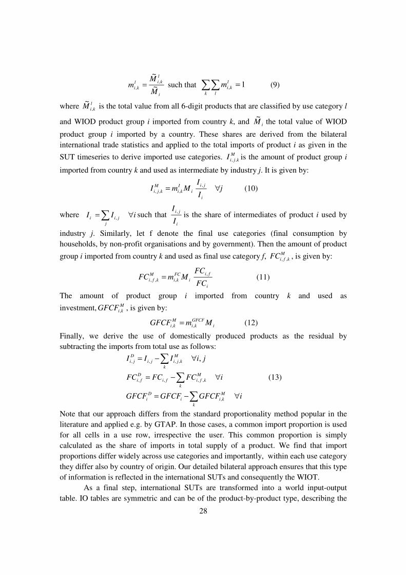
28

i

l

kil

kiM

Mm ~

~,

, = such that 1, =∑∑k l

l

kim (9)

where l

kiM ,

~ is the total value from all 6-digit products that are classified by use category l

and WIOD product group i imported from country k, and iM~

the total value of WIOD

product group i imported by a country. These shares are derived from the bilateral

international trade statistics and applied to the total imports of product i as given in the

SUT timeseries to derive imported use categories. M

kjiI ,, is the amount of product group i

imported from country k and used as intermediate by industry j. It is given by:

jI

IMmI

i

ji

i

I

ki

M

kji ∀=,

,,, (10)

where iIIj

jii ∀=∑ ,such that

i

ji

I

I ,is the share of intermediates of product i used by

industry j. Similarly, let f denote the final use categories (final consumption by

households, by non-profit organisations and by government). Then the amount of product

group i imported from country k and used as final use category f, M

kfiFC ,, , is given by:

i

fi

i

CF

ki

M

kfiFC

FCMmFC

,

,,, = (11)

The amount of product group i imported from country k and used as

investment, M

kiGFCF , , is given by:

i

GFCF

ki

M

ki MmGFCF ,, = (12)

Finally, we derive the use of domestically produced products as the residual by

subtracting the imports from total use as follows:

iGFCFGFCFGFCF

iFCFCFC

jiIII

k

M

kii

D

i

k

M

kfifi

D

fi

k

M

kjiji

D

ji

∀−=

∀−=

∀−=

∑

∑

∑

,

,,,,

,,,, ,

(13)

Note that our approach differs from the standard proportionality method popular in the

literature and applied e.g. by GTAP. In those cases, a common import proportion is used

for all cells in a use row, irrespective the user. This common proportion is simply

calculated as the share of imports in total supply of a product. We find that import

proportions differ widely across use categories and importantly, within each use category

they differ also by country of origin. Our detailed bilateral approach ensures that this type

of information is reflected in the international SUTs and consequently the WIOT.

As a final step, international SUTs are transformed into a world input-output

table. IO tables are symmetric and can be of the product-by-product type, describing the

29

amount of products needed to produce a particular good or service, or of the industry-by-

industry type, describing the flow of goods and services from one industry to another. In

case each product is only produced by one industry, the two types of tables will be the

same. But the larger the share of secondary production, the larger the difference will be.

The choice for between the two depends on the type of research questions. Many foreseen

applications of the WIOT, such as those described in the next sections, will rely heavily

on industry-type tables as the additional data, such as employment or investment, is often

only available on an industry basis. Moreover, the industry-type table retains best the

links with national account statistics.

An IOT is a construct on the basis of a SUT at basic prices based on additional

assumptions concerning technology. We use the so-called “fixed product-sales structure”

assumption stating that each product has its own specific sales structure irrespective of

the industry where it is produced. Sales structure here refers to the proportions of the

output of the product in which it is sold to the respective intermediate and final users.

This assumption is most widely used, not only because it is more realistic than its

alternatives, but also because it requires a relative simple mechanical procedure.

Furthermore, it does not generate any negatives in the IOT that would require manual

rebalancing. Application of manual ad-hoc procedures would greatly reduce the

tractability of our methods. Chapter 11 in the Eurostat handbook (Eurostat, 2008)

provides a useful and extensive discussion of the transformation of SUTs into IOTs,

including a mathematical treatment.

The full WIOT will contain data for forty countries covered in the WIOD.

Including the biggest countries in the world, this set covers more than 85 per cent of

world GDP. Nevertheless to complete the WIOT and make it suitable for various

modelling purposes, we also added a region called the Rest of the World (RoW) that

proxies for all other countries in the world. The RoW needs to be modelled due to a lack

of detailed data on input-output structures. Imports from RoW are given as as share of

imports from RoW from trade data applied to the imports in the supply table. Hence,

exports from the RoW are simply the imports by our set of countries not originating from

the set of WIOD countries. Exports to RoW from the set of WIOD countries or,

equivalently, imports by the ROW are defined residually to ensure that exports from all

countries (incl. RoW) equal the imports by all countries (incl. RoW). Production and

consumption in the ROW will be modelled based on totals for industry output and final

use categories from the UN National Accounts, assuming an input-output structure equal

to that of an average developing country. Also, at a later stage we will add in a separate

oil-producing region that will be useful in particular in environmental applications.

For an elaborate discussion of construction methods, practical implementation and

detailed sources of the WIOT, see Erumban et al. (2011, forthcoming).

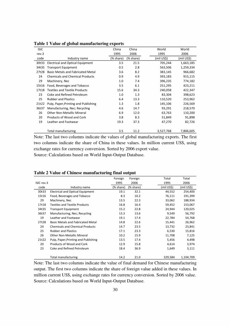
30

Table 1 Value of global manufacturing exports China China World World

1995 2006 1995 2006

Industry name (% share) (% share) (mil US$) (mil US$)

30t33 Electrical and Optical Equipment 3.5 21.5 705,244 1,663,185

34t35 Transport Equipment 0.5 2.8 563,506 1,259,334

27t28 Basic Metals and Fabricated Metal 3.6 8.2 383,145 966,682

24 Chemicals and Chemical Products 0.9 4.9 393,183 915,115

29 Machinery, Nec 1.0 7.4 396,235 774,182

15t16 Food, Beverages and Tobacco 3.5 6.1 251,295 423,211

17t18 Textiles and Textile Products 15.6 34.3 240,058 422,347

23 Coke and Refined Petroleum 1.0 1.3 83,304 398,623

25 Rubber and Plastics 6.4 13.3 110,520 253,962

21t22 Pulp, Paper,Printing and Publishing 1.3 1.8 145,106 226,569

36t37 Manufacturing, Nec; Recycling 4.6 14.7 93,291 218,570

26 Other Non-Metallic Mineral 6.9 12.0 63,763 110,200

20 Products of Wood and Cork 3.8 8.3 51,849 91,898

19 Leather and Footwear 19.3 37.3 47,270 82,726

Total manufacturing 3.5 11.2 3,527,768 7,806,605

ISIC

rev.3

code

Note: The last two columns indicate the values of global manufacturing exports. The first

two columns indicate the share of China in these values. In million current US$, using

exchange rates for currency conversion. Sorted by 2006 export value.

Source: Calculations based on World Input-Output Database.

Table 2 Value of Chinese manufacturing final output Foreign Foreign Total Total

1995 2006 1995 2006

Industry name (% share) (% share) (mil US$) (mil US$)

30t33 Electrical and Optical Equipment 19.1 32.1 44,552 254,400

15t16 Food, Beverages and Tobacco 8.3 10.2 76,111 191,399

29 Machinery, Nec 13.5 22.3 33,062 188,934

17t18 Textiles and Textile Products 16.8 16.4 59,452 153,067

34t35 Transport Equipment 15.2 22.8 24,944 120,025

36t37 Manufacturing, Nec; Recycling 13.3 13.6 9,549 56,792

19 Leather and Footwear 19.1 17.4 22,784 54,768

27t28 Basic Metals and Fabricated Metal 14.8 22.6 15,441 26,962

24 Chemicals and Chemical Products 14.7 23.5 13,732 23,841

25 Rubber and Plastics 17.1 23.3 6,530 15,816

26 Other Non-Metallic Mineral 10.2 15.9 11,708 7,125

21t22 Pulp, Paper,Printing and Publishing 13.5 17.4 5,456 4,498

20 Products of Wood and Cork 12.9 15.8 4,614 3,974

23 Coke and Refined Petroleum 18.4 36.9 1,649 3,111

Total manufacturing 14.2 21.0 329,584 1,104,709

ISIC rev.3

code

Note: The last two columns indicate the value of final demand for Chinese manufacturing

output. The first two columns indicate the share of foreign value added in these values. In

million current US$, using exchange rates for currency conversion. Sorted by 2006 value.

Source: Calculations based on World Input-Output Database.

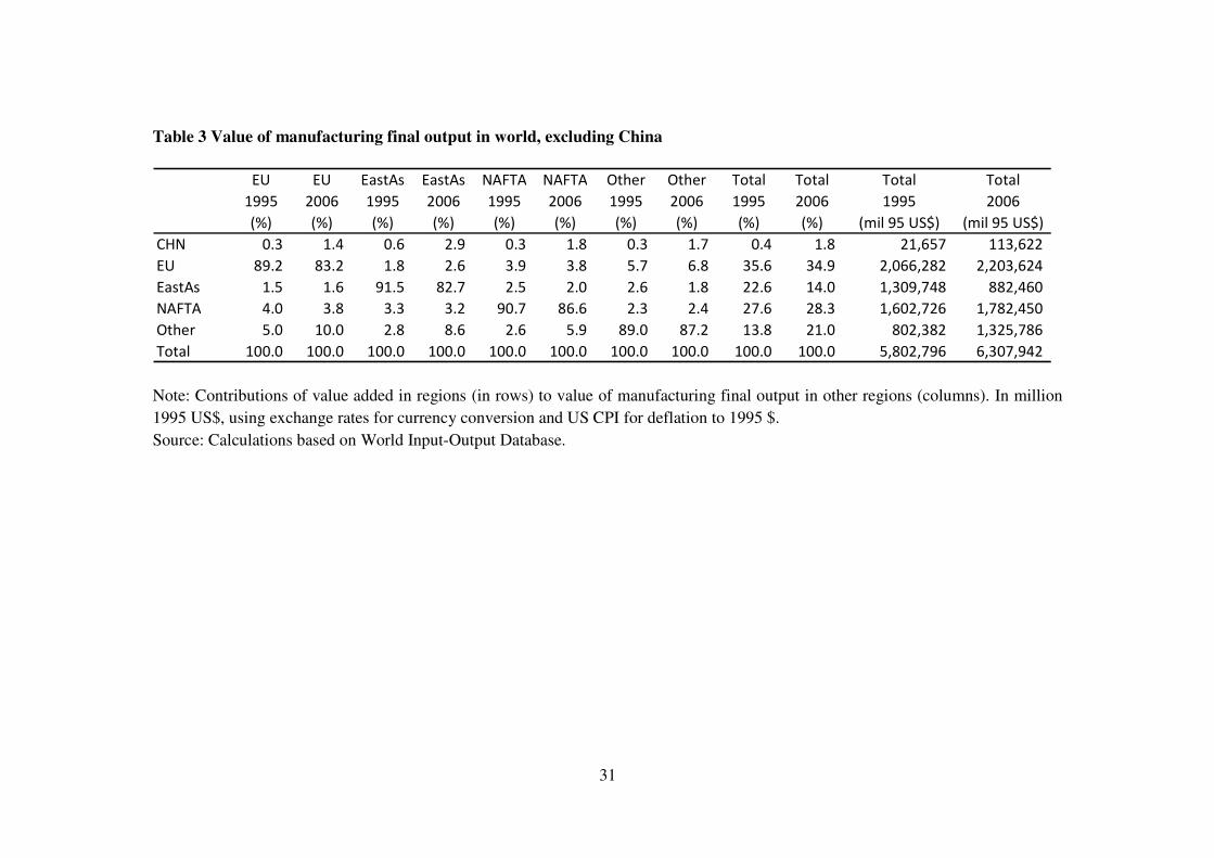
31

Table 3 Value of manufacturing final output in world, excluding China

EU EU EastAs EastAs NAFTA NAFTA Other Other Total Total Total Total

1995 2006 1995 2006 1995 2006 1995 2006 1995 2006 1995 2006

(%) (%) (%) (%) (%) (%) (%) (%) (%) (%) (mil 95 US$) (mil 95 US$)

CHN 0.3 1.4 0.6 2.9 0.3 1.8 0.3 1.7 0.4 1.8 21,657 113,622

EU 89.2 83.2 1.8 2.6 3.9 3.8 5.7 6.8 35.6 34.9 2,066,282 2,203,624

EastAs 1.5 1.6 91.5 82.7 2.5 2.0 2.6 1.8 22.6 14.0 1,309,748 882,460

NAFTA 4.0 3.8 3.3 3.2 90.7 86.6 2.3 2.4 27.6 28.3 1,602,726 1,782,450

Other 5.0 10.0 2.8 8.6 2.6 5.9 89.0 87.2 13.8 21.0 802,382 1,325,786

Total 100.0 100.0 100.0 100.0 100.0 100.0 100.0 100.0 100.0 100.0 5,802,796 6,307,942

Note: Contributions of value added in regions (in rows) to value of manufacturing final output in other regions (columns). In million

1995 US$, using exchange rates for currency conversion and US CPI for deflation to 1995 $.

Source: Calculations based on World Input-Output Database.

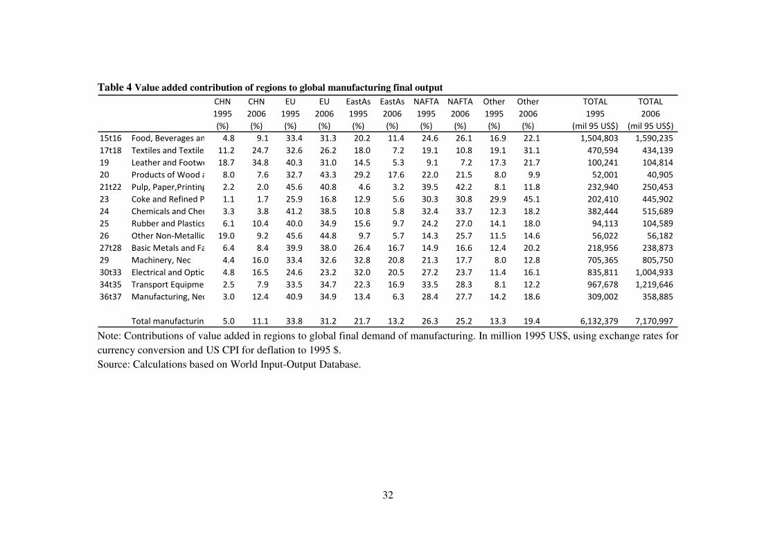
32

Table 4 Value added contribution of regions to global manufacturing final output

CHN CHN EU EU EastAs EastAs NAFTA NAFTA Other Other TOTAL TOTAL

1995 2006 1995 2006 1995 2006 1995 2006 1995 2006 1995 2006

(%) (%) (%) (%) (%) (%) (%) (%) (%) (%) (mil 95 US$) (mil 95 US$)

15t16 Food, Beverages and Tobacco4.8 9.1 33.4 31.3 20.2 11.4 24.6 26.1 16.9 22.1 1,504,803 1,590,235

17t18 Textiles and Textile Products11.2 24.7 32.6 26.2 18.0 7.2 19.1 10.8 19.1 31.1 470,594 434,139

19 Leather and Footwear 18.7 34.8 40.3 31.0 14.5 5.3 9.1 7.2 17.3 21.7 100,241 104,814

20 Products of Wood and Cork8.0 7.6 32.7 43.3 29.2 17.6 22.0 21.5 8.0 9.9 52,001 40,905

21t22 Pulp, Paper,Printing and Publishing2.2 2.0 45.6 40.8 4.6 3.2 39.5 42.2 8.1 11.8 232,940 250,453

23 Coke and Refined Petroleum1.1 1.7 25.9 16.8 12.9 5.6 30.3 30.8 29.9 45.1 202,410 445,902

24 Chemicals and Chemical Products3.3 3.8 41.2 38.5 10.8 5.8 32.4 33.7 12.3 18.2 382,444 515,689

25 Rubber and Plastics 6.1 10.4 40.0 34.9 15.6 9.7 24.2 27.0 14.1 18.0 94,113 104,589

26 Other Non-Metallic Mineral19.0 9.2 45.6 44.8 9.7 5.7 14.3 25.7 11.5 14.6 56,022 56,182

27t28 Basic Metals and Fabricated Metal6.4 8.4 39.9 38.0 26.4 16.7 14.9 16.6 12.4 20.2 218,956 238,873

29 Machinery, Nec 4.4 16.0 33.4 32.6 32.8 20.8 21.3 17.7 8.0 12.8 705,365 805,750

30t33 Electrical and Optical Equipment4.8 16.5 24.6 23.2 32.0 20.5 27.2 23.7 11.4 16.1 835,811 1,004,933

34t35 Transport Equipment 2.5 7.9 33.5 34.7 22.3 16.9 33.5 28.3 8.1 12.2 967,678 1,219,646

36t37 Manufacturing, Nec; Recycling3.0 12.4 40.9 34.9 13.4 6.3 28.4 27.7 14.2 18.6 309,002 358,885

Total manufacturing 5.0 11.1 33.8 31.2 21.7 13.2 26.3 25.2 13.3 19.4 6,132,379 7,170,997 Note: Contributions of value added in regions to global final demand of manufacturing. In million 1995 US$, using exchange rates for

currency conversion and US CPI for deflation to 1995 $.

Source: Calculations based on World Input-Output Database.

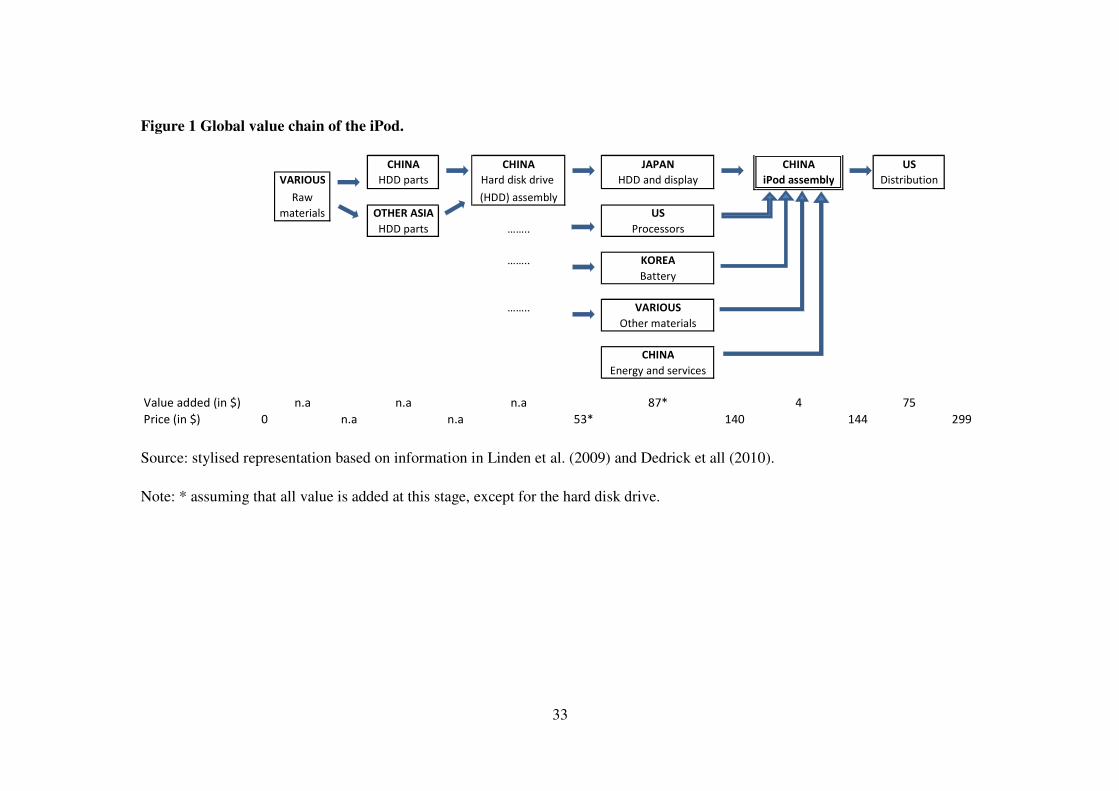
33

Figure 1 Global value chain of the iPod.

CHINA CHINA JAPAN CHINA US

VARIOUS HDD parts Hard disk drive HDD and display iPod assembly Distribution

(HDD) assembly

OTHER ASIA US

HDD parts …….. Processors

…….. KOREA

Battery

…….. VARIOUS

Other materials

CHINA

Energy and services

Value added (in $) n.a n.a n.a 87* 4 75

Price (in $) 0 n.a n.a 53* 140 144 299

Raw

materials

Source: stylised representation based on information in Linden et al. (2009) and Dedrick et all (2010).

Note: * assuming that all value is added at this stage, except for the hard disk drive.

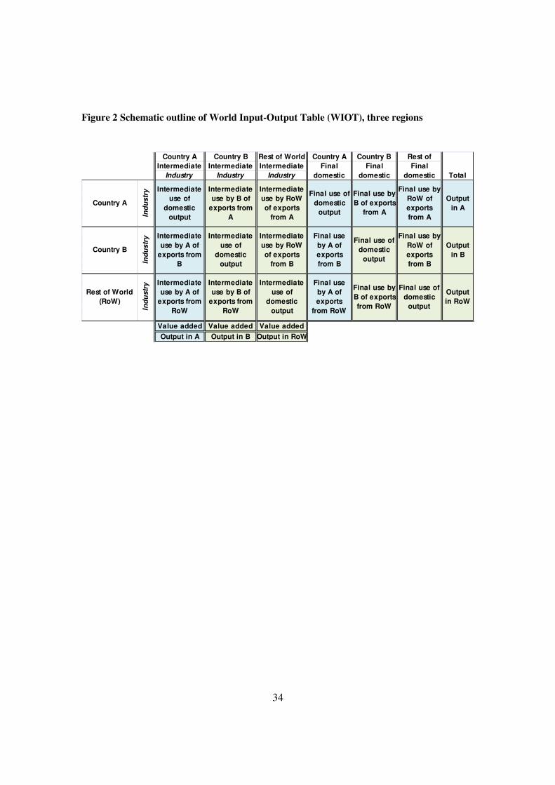
34

Figure 2 Schematic outline of World Input-Output Table (WIOT), three regions

Country A Country B Rest of World Country A Country B Rest of

Total

Intermediate Intermediate Intermediate Final

domestic

Final

domestic

Final

domestic Industry Industry Industry

Country A

Ind

ustr

y Intermediate

use of

domestic

output

Intermediate

use by B of

exports from

A

Intermediate

use by RoW

of exports

from A

Final use of

domestic

output

Final use by

B of exports

from A

Final use by

RoW of

exports

from A

Output

in A

Country B

Ind

ustr

y Intermediate

use by A of

exports from

B

Intermediate

use of

domestic

output

Intermediate

use by RoW

of exports

from B

Final use

by A of

exports

from B

Final use of

domestic

output

Final use by

RoW of

exports

from B

Output

in B

Rest of World

(RoW)

Ind

ustr

y Intermediate

use by A of

exports from

RoW

Intermediate

use by B of

exports from

RoW

Intermediate

use of

domestic

output

Final use

by A of

exports

from RoW

Final use by

B of exports

from RoW

Final use of

domestic

output

Output

in RoW

Value added Value added Value added

Output in A Output in B Output in RoW

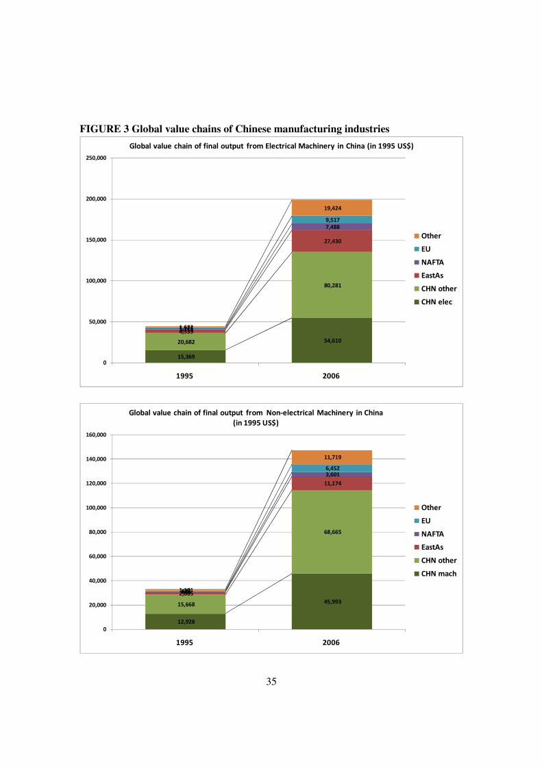
35

FIGURE 3 Global value chains of Chinese manufacturing industries

15,369

54,610 20,682

80,281

4,539

27,430

1,218

7,488

1,121

9,517

1,622

19,424

0

50,000

100,000

150,000

200,000

250,000

1995 2006

Global value chain of final output from Electrical Machinery in China (in 1995 US$)

Other

EU

NAFTA

EastAs

CHN other

CHN elec

12,928

45,993 15,668

68,665

2,065

11,174

606

3,601

695

6,452

1,101

11,719

0

20,000

40,000

60,000

80,000

100,000

120,000

140,000

160,000

1995 2006

Global value chain of final output from Non-electrical Machinery in China

(in 1995 US$)

Other

EU

NAFTA

EastAs

CHN other

CHN mach

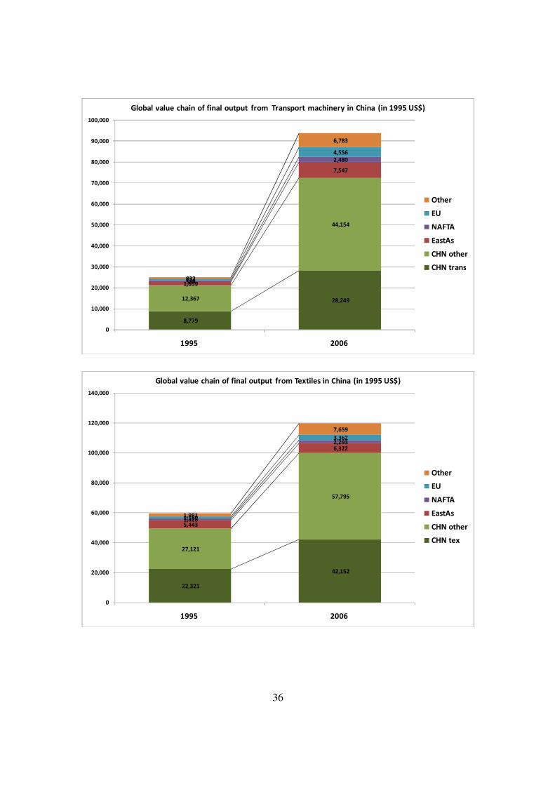
36

8,779

28,249 12,367

44,154

1,659

7,547

584

2,480

724

4,556

832

6,783

0

10,000

20,000

30,000

40,000

50,000

60,000

70,000

80,000

90,000

100,000

1995 2006

Global value chain of final output from Transport machinery in China (in 1995 US$)

Other

EU

NAFTA

EastAs

CHN other

CHN trans

22,321

42,152

27,121

57,795

5,443

6,322

1,426

2,293

1,160

3,362

1,981

7,659

0

20,000

40,000

60,000

80,000

100,000

120,000

140,000

1995 2006

Global value chain of final output from Textiles in China (in 1995 US$)

Other

EU

NAFTA

EastAs

CHN other

CHN tex

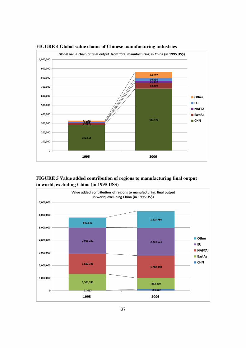
37

FIGURE 4 Global value chains of Chinese manufacturing industries

282,661

681,673

21,403

62,259

7,902

21,432

6,470

30,994

11,148

66,697

0

100,000

200,000

300,000

400,000

500,000

600,000

700,000

800,000

900,000

1,000,000

1995 2006

Global value chain of final output from Total manufacturing in China (in 1995 US$)

Other

EU

NAFTA

EastAs

CHN

FIGURE 5 Value added contribution of regions to manufacturing final output

in world, excluding China (in 1995 US$)

21,657 113,622

1,309,748 882,460

1,602,726 1,782,450

2,066,282 2,203,624

802,382 1,325,786

0

1,000,000

2,000,000

3,000,000

4,000,000

5,000,000

6,000,000

7,000,000

1995 2006

Value added contribution of regions to manufacturing final output

in world, excluding China (in 1995 US$)

Other

EU

NAFTA

EastAs

CHN

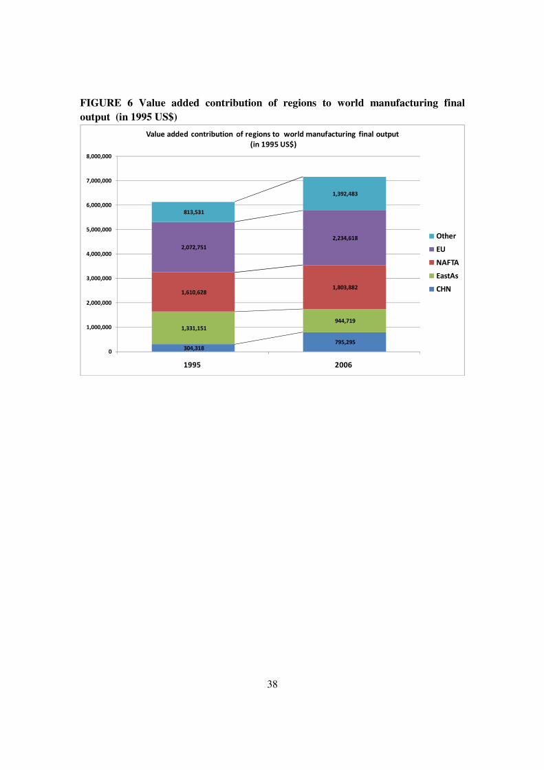
38

FIGURE 6 Value added contribution of regions to world manufacturing final

output (in 1995 US$)

304,318 795,295

1,331,151

944,719

1,610,628 1,803,882

2,072,751

2,234,618

813,531

1,392,483

0

1,000,000

2,000,000

3,000,000

4,000,000

5,000,000

6,000,000

7,000,000

8,000,000

1995 2006

Value added contribution of regions to world manufacturing final output

(in 1995 US$)

Other

EU

NAFTA

EastAs

CHN

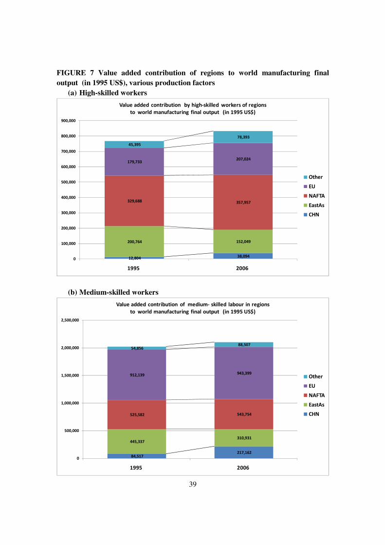
39

FIGURE 7 Value added contribution of regions to world manufacturing final

output (in 1995 US$), various production factors

(a) High-skilled workers

12,804 38,094

200,764 152,049

329,688 357,957

179,733 207,024

45,395

78,393

0

100,000

200,000

300,000

400,000

500,000

600,000

700,000

800,000

900,000

1995 2006

Value added contribution by high-skilled workers of regions

to world manufacturing final output (in 1995 US$)

Other

EU

NAFTA

EastAs

CHN

(b) Medium-skilled workers

84,517 217,162

445,337 310,931

525,582 543,754

912,139 943,399

54,856 88,507

0

500,000

1,000,000

1,500,000

2,000,000

2,500,000

1995 2006

Value added contribution of medium- skilled labour in regions

to world manufacturing final output (in 1995 US$)

Other

EU

NAFTA

EastAs

CHN

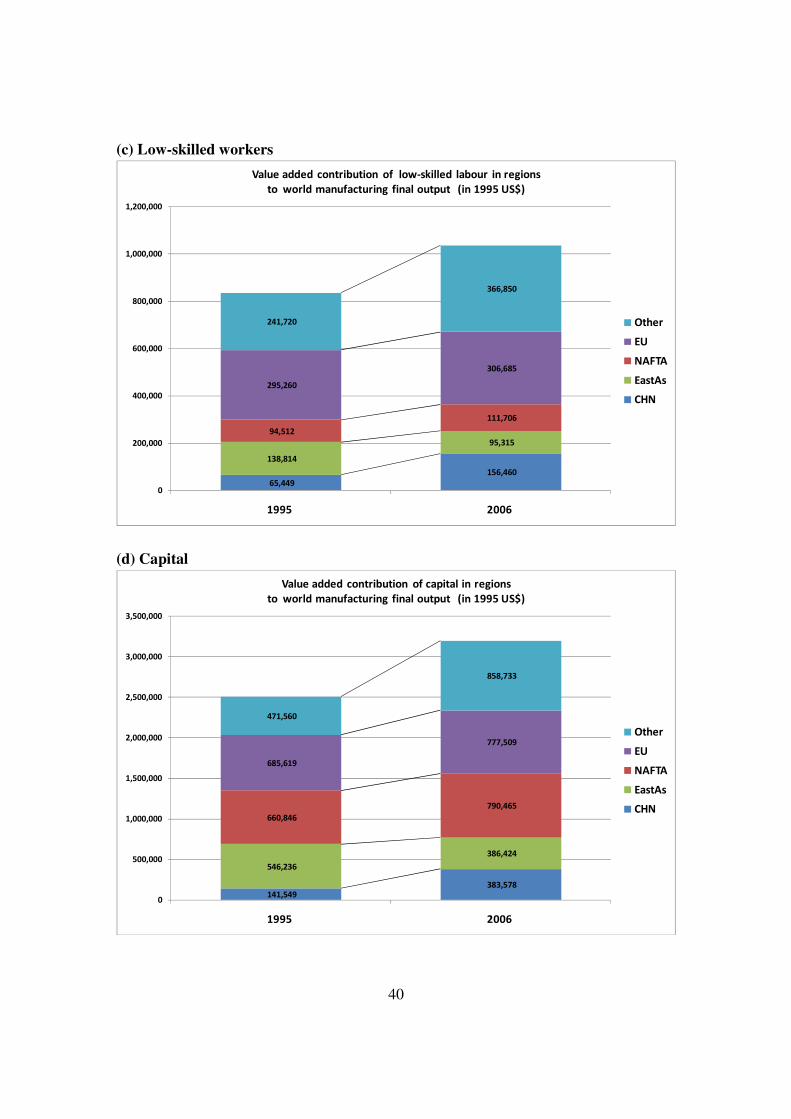
40

(c) Low-skilled workers

65,449

156,460

138,814

95,315

94,512

111,706

295,260

306,685

241,720

366,850

0

200,000

400,000

600,000

800,000

1,000,000

1,200,000

1995 2006

Value added contribution of low-skilled labour in regions

to world manufacturing final output (in 1995 US$)

Other

EU

NAFTA

EastAs

CHN

(d) Capital

141,549 383,578

546,236

386,424

660,846

790,465

685,619

777,509

471,560

858,733

0

500,000

1,000,000

1,500,000

2,000,000

2,500,000

3,000,000

3,500,000

1995 2006

Value added contribution of capital in regions

to world manufacturing final output (in 1995 US$)

Other

EU

NAFTA

EastAs

CHN

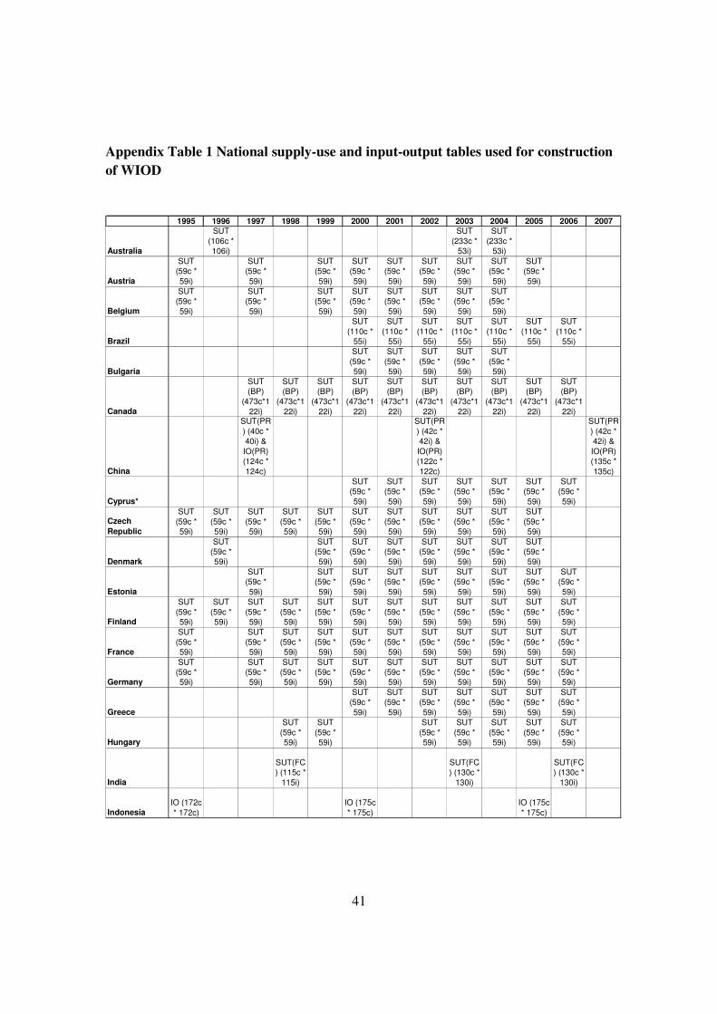
41

Appendix Table 1 National supply-use and input-output tables used for construction

of WIOD

1995 1996 1997 1998 1999 2000 2001 2002 2003 2004 2005 2006 2007

Australia

SUT

(106c *

106i)

SUT

(233c *

53i)

SUT

(233c *

53i)

Austria

SUT

(59c *

59i)

SUT

(59c *

59i)

SUT

(59c *

59i)

SUT

(59c *

59i)

SUT

(59c *

59i)

SUT

(59c *

59i)

SUT

(59c *

59i)

SUT

(59c *

59i)

SUT

(59c *

59i)

Belgium

SUT

(59c *

59i)

SUT

(59c *

59i)

SUT

(59c *

59i)

SUT

(59c *

59i)

SUT

(59c *

59i)

SUT

(59c *

59i)

SUT

(59c *

59i)

SUT

(59c *

59i)

Brazil

SUT

(110c *

55i)

SUT

(110c *

55i)

SUT

(110c *

55i)

SUT

(110c *

55i)

SUT

(110c *

55i)

SUT

(110c *

55i)

SUT

(110c *

55i)

Bulgaria

SUT

(59c *

59i)

SUT

(59c *

59i)

SUT

(59c *

59i)

SUT

(59c *

59i)

SUT

(59c *

59i)

Canada

SUT

(BP)

(473c*1

22i)

SUT

(BP)

(473c*1

22i)

SUT

(BP)

(473c*1

22i)

SUT

(BP)

(473c*1

22i)

SUT

(BP)

(473c*1

22i)

SUT

(BP)

(473c*1

22i)

SUT

(BP)

(473c*1

22i)

SUT

(BP)

(473c*1

22i)

SUT

(BP)

(473c*1

22i)

SUT

(BP)

(473c*1

22i)

China

SUT(PR

) (40c *

40i) &

IO(PR)

(124c *

124c)

SUT(PR

) (42c *

42i) &

IO(PR)

(122c *

122c)

SUT(PR

) (42c *

42i) &

IO(PR)

(135c *

135c)

Cyprus*

SUT

(59c *

59i)

SUT

(59c *

59i)

SUT

(59c *

59i)

SUT

(59c *

59i)

SUT

(59c *

59i)

SUT

(59c *

59i)

SUT

(59c *

59i)

Czech

Republic

SUT

(59c *

59i)

SUT

(59c *

59i)

SUT

(59c *

59i)

SUT

(59c *

59i)

SUT

(59c *

59i)

SUT

(59c *

59i)

SUT

(59c *

59i)

SUT

(59c *

59i)

SUT

(59c *

59i)

SUT

(59c *

59i)

SUT

(59c *

59i)

Denmark

SUT

(59c *

59i)

SUT

(59c *

59i)

SUT

(59c *

59i)

SUT

(59c *

59i)

SUT

(59c *

59i)

SUT

(59c *

59i)

SUT

(59c *

59i)

SUT

(59c *

59i)

Estonia

SUT

(59c *

59i)

SUT

(59c *

59i)

SUT

(59c *

59i)

SUT

(59c *

59i)

SUT

(59c *

59i)

SUT

(59c *

59i)

SUT

(59c *

59i)

SUT

(59c *

59i)

SUT

(59c *

59i)

Finland

SUT

(59c *

59i)

SUT

(59c *

59i)

SUT

(59c *

59i)

SUT

(59c *

59i)

SUT

(59c *

59i)

SUT

(59c *

59i)

SUT

(59c *

59i)

SUT

(59c *

59i)

SUT

(59c *

59i)

SUT

(59c *

59i)

SUT

(59c *

59i)

SUT

(59c *

59i)

France

SUT

(59c *

59i)

SUT

(59c *

59i)

SUT

(59c *

59i)

SUT

(59c *

59i)

SUT

(59c *

59i)

SUT

(59c *

59i)

SUT

(59c *

59i)

SUT

(59c *

59i)

SUT

(59c *

59i)

SUT

(59c *

59i)

SUT

(59c *

59i)

Germany

SUT

(59c *

59i)

SUT

(59c *

59i)

SUT

(59c *

59i)

SUT

(59c *

59i)

SUT

(59c *

59i)

SUT

(59c *

59i)

SUT

(59c *

59i)

SUT

(59c *

59i)

SUT

(59c *

59i)

SUT

(59c *

59i)

SUT

(59c *

59i)

Greece

SUT

(59c *

59i)

SUT

(59c *

59i)

SUT

(59c *

59i)

SUT

(59c *

59i)

SUT

(59c *

59i)

SUT

(59c *

59i)

SUT

(59c *

59i)

Hungary

SUT

(59c *

59i)

SUT

(59c *

59i)

SUT

(59c *

59i)

SUT

(59c *

59i)

SUT

(59c *

59i)

SUT

(59c *

59i)

SUT

(59c *

59i)

India

SUT(FC

) (115c *

115i)

SUT(FC

) (130c *

130i)

SUT(FC

) (130c *

130i)

Indonesia

IO (172c

* 172c)

IO (175c

* 175c)

IO (175c

* 175c)

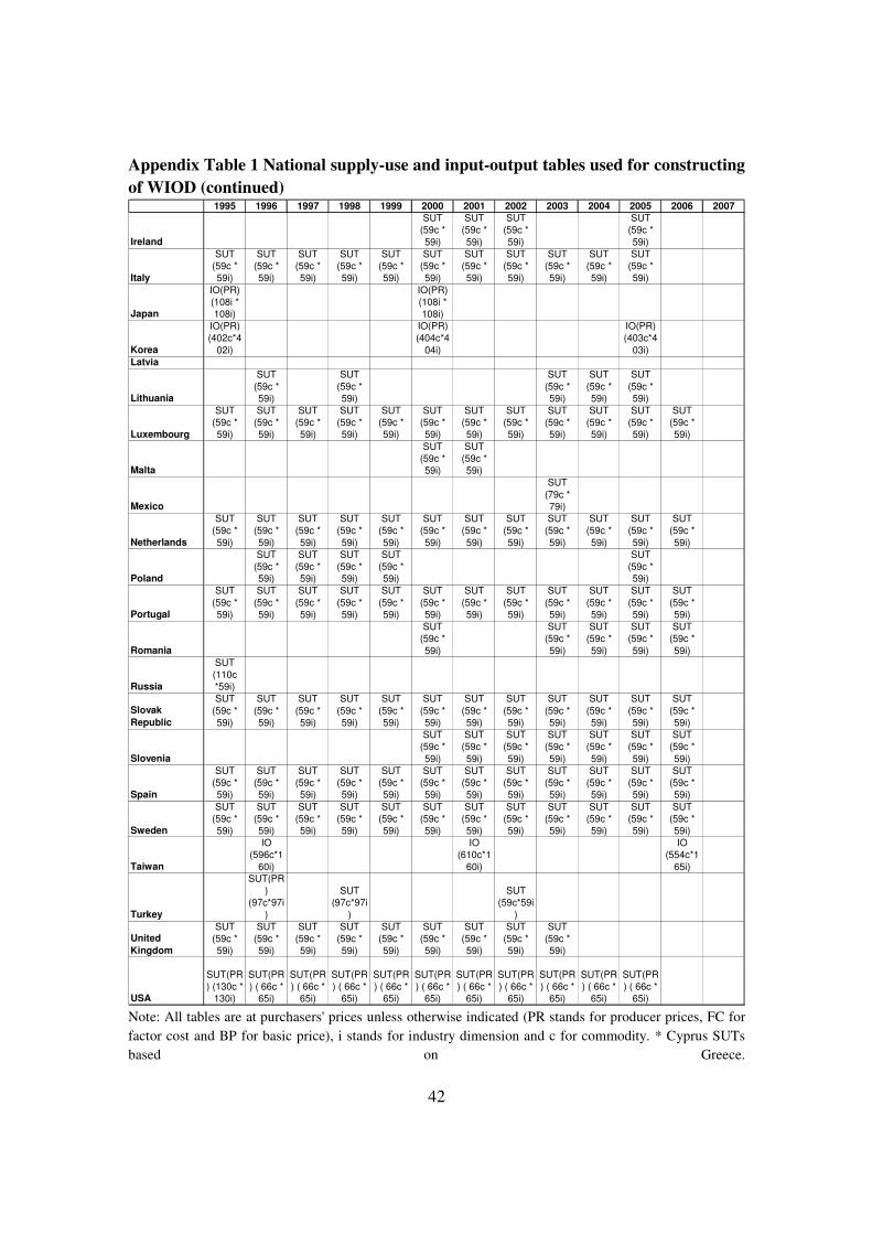
42

Appendix Table 1 National supply-use and input-output tables used for constructing

of WIOD (continued) 1995 1996 1997 1998 1999 2000 2001 2002 2003 2004 2005 2006 2007

Ireland

SUT

(59c *

59i)

SUT

(59c *

59i)

SUT

(59c *

59i)

SUT

(59c *

59i)

Italy

SUT

(59c *

59i)

SUT

(59c *

59i)

SUT

(59c *

59i)

SUT

(59c *

59i)

SUT

(59c *

59i)

SUT

(59c *

59i)

SUT

(59c *

59i)

SUT

(59c *

59i)

SUT

(59c *

59i)

SUT

(59c *

59i)

SUT

(59c *

59i)

Japan

IO(PR)

(108i *

108i)

IO(PR)

(108i *

108i)

Korea

IO(PR)

(402c*4

02i)

IO(PR)

(404c*4

04i)

IO(PR)

(403c*4

03i)

Latvia

Lithuania

SUT

(59c *

59i)

SUT

(59c *

59i)

SUT

(59c *

59i)

SUT

(59c *

59i)

SUT

(59c *

59i)

Luxembourg

SUT

(59c *

59i)

SUT

(59c *

59i)

SUT

(59c *

59i)

SUT

(59c *

59i)

SUT

(59c *

59i)

SUT

(59c *

59i)

SUT

(59c *

59i)

SUT

(59c *

59i)

SUT

(59c *

59i)

SUT

(59c *

59i)

SUT

(59c *

59i)

SUT

(59c *

59i)

Malta

SUT

(59c *

59i)

SUT

(59c *

59i)

Mexico

SUT

(79c *

79i)

Netherlands

SUT

(59c *

59i)

SUT

(59c *

59i)

SUT

(59c *

59i)

SUT

(59c *

59i)

SUT

(59c *

59i)

SUT

(59c *

59i)

SUT

(59c *

59i)

SUT

(59c *

59i)

SUT

(59c *

59i)

SUT

(59c *

59i)

SUT

(59c *

59i)

SUT

(59c *

59i)

Poland

SUT

(59c *

59i)

SUT

(59c *

59i)

SUT

(59c *

59i)

SUT

(59c *

59i)

SUT

(59c *

59i)

Portugal

SUT

(59c *

59i)

SUT

(59c *

59i)

SUT

(59c *

59i)

SUT

(59c *

59i)

SUT

(59c *

59i)

SUT

(59c *

59i)

SUT

(59c *

59i)

SUT

(59c *

59i)

SUT

(59c *

59i)

SUT

(59c *

59i)

SUT

(59c *

59i)

SUT

(59c *

59i)

Romania

SUT

(59c *

59i)

SUT

(59c *

59i)

SUT

(59c *

59i)

SUT

(59c *

59i)

SUT

(59c *

59i)

Russia

SUT

(110c

*59i)

Slovak

Republic

SUT

(59c *

59i)

SUT

(59c *

59i)

SUT

(59c *

59i)

SUT

(59c *

59i)

SUT

(59c *

59i)

SUT

(59c *

59i)

SUT

(59c *

59i)

SUT

(59c *

59i)

SUT

(59c *

59i)

SUT

(59c *

59i)

SUT

(59c *

59i)

SUT

(59c *

59i)

Slovenia

SUT

(59c *

59i)

SUT

(59c *

59i)

SUT

(59c *

59i)

SUT

(59c *

59i)

SUT

(59c *

59i)

SUT

(59c *

59i)

SUT

(59c *

59i)

Spain

SUT

(59c *

59i)

SUT

(59c *

59i)

SUT

(59c *

59i)

SUT

(59c *

59i)

SUT

(59c *

59i)

SUT

(59c *

59i)

SUT

(59c *

59i)

SUT

(59c *

59i)

SUT

(59c *

59i)

SUT

(59c *

59i)

SUT

(59c *

59i)

SUT

(59c *

59i)

Sweden

SUT

(59c *

59i)

SUT

(59c *

59i)

SUT

(59c *

59i)

SUT

(59c *

59i)

SUT

(59c *

59i)

SUT

(59c *

59i)

SUT

(59c *

59i)

SUT

(59c *

59i)

SUT

(59c *

59i)

SUT

(59c *

59i)

SUT

(59c *

59i)

SUT

(59c *

59i)

Taiwan

IO

(596c*1

60i)

IO

(610c*1

60i)

IO

(554c*1

65i)

Turkey

SUT(PR

)

(97c*97i

)

SUT

(97c*97i

)

SUT

(59c*59i

)

United

Kingdom

SUT

(59c *

59i)

SUT

(59c *

59i)

SUT

(59c *

59i)

SUT

(59c *

59i)

SUT

(59c *

59i)

SUT

(59c *

59i)

SUT

(59c *

59i)

SUT

(59c *

59i)

SUT

(59c *

59i)

USA

SUT(PR

) (130c *

130i)

SUT(PR

) ( 66c *

65i)

SUT(PR

) ( 66c *

65i)

SUT(PR

) ( 66c *

65i)

SUT(PR

) ( 66c *

65i)

SUT(PR

) ( 66c *

65i)

SUT(PR

) ( 66c *

65i)

SUT(PR

) ( 66c *

65i)

SUT(PR

) ( 66c *

65i)

SUT(PR

) ( 66c *

65i)

SUT(PR

) ( 66c *

65i) Note: All tables are at purchasers' prices unless otherwise indicated (PR stands for producer prices, FC for

factor cost and BP for basic price), i stands for industry dimension and c for commodity. * Cyprus SUTs

based on Greece.

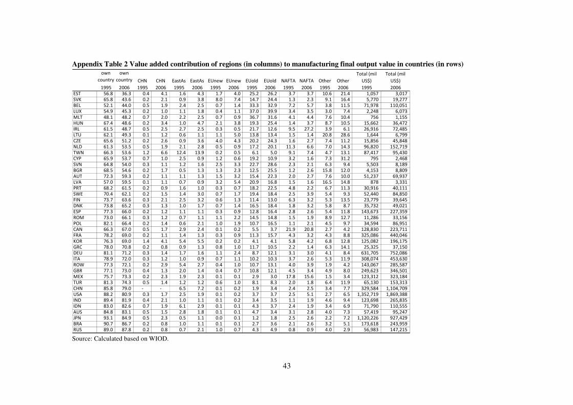
43

Appendix Table 2 Value added contribution of regions (in columns) to manufacturing final output value in countries (in rows) own

country

own

country CHN CHN EastAs EastAs EUnew EUnew EUold EUold NAFTA NAFTA Other Other

Total (mil

US$)

Total (mil

US$)

1995 2006 1995 2006 1995 2006 1995 2006 1995 2006 1995 2006 1995 2006 1995 2006EST 56.8 36.3 0.4 4.1 1.6 4.3 1.7 4.0 25.2 26.2 3.7 3.7 10.6 21.4 1,057 3,017 SVK 65.8 43.6 0.2 2.1 0.9 3.8 8.0 7.4 14.7 24.4 1.3 2.3 9.1 16.4 5,770 19,277 BEL 52.1 44.0 0.5 1.9 2.4 2.5 0.7 1.4 33.3 32.9 7.2 5.7 3.8 11.5 71,978 110,051 LUX 54.9 45.3 0.2 1.0 1.1 1.8 0.4 1.1 37.0 39.9 3.4 3.5 3.0 7.4 2,248 6,073 MLT 48.1 48.2 0.7 2.0 2.2 2.5 0.7 0.9 36.7 31.6 4.1 4.4 7.6 10.4 756 1,155 HUN 67.4 48.6 0.2 3.4 1.0 4.7 2.1 3.8 19.3 25.4 1.4 3.7 8.7 10.5 15,662 36,472 IRL 61.5 48.7 0.5 2.5 2.7 2.5 0.3 0.5 21.7 12.6 9.5 27.2 3.9 6.1 26,916 72,485 LTU 62.1 49.3 0.1 1.2 0.6 1.1 1.1 5.0 13.8 13.4 1.5 1.4 20.8 28.6 1,644 6,799 CZE 65.6 51.2 0.2 2.6 0.9 3.6 4.0 4.3 20.2 24.3 1.6 2.7 7.4 11.2 15,856 45,848 NLD 61.3 53.5 0.5 1.9 2.1 2.8 0.5 0.9 17.2 20.1 11.3 6.6 7.0 14.3 96,820 152,719 TWN 66.3 53.6 1.2 6.6 12.4 13.9 0.2 0.5 6.1 5.0 9.1 7.4 4.7 13.1 87,417 95,430 CYP 65.9 53.7 0.7 1.0 2.5 0.9 1.2 0.6 19.2 10.9 3.2 1.6 7.3 31.2 795 2,468 SVN 64.8 54.0 0.3 1.1 1.2 1.6 2.5 3.3 22.7 28.6 2.3 2.1 6.3 9.4 5,503 8,189 BGR 68.5 54.6 0.2 1.7 0.5 1.3 1.3 2.3 12.5 25.5 1.2 2.6 15.8 12.0 4,153 8,809 AUT 72.3 59.3 0.2 1.1 1.1 1.3 1.5 3.2 15.4 22.3 2.0 2.7 7.6 10.0 51,237 69,937 LVA 57.0 59.5 0.1 1.1 0.7 0.9 3.2 5.4 20.9 16.8 1.5 1.6 16.5 14.8 878 3,331 PRT 68.2 61.5 0.2 0.9 1.6 1.0 0.3 0.7 18.2 22.5 4.8 2.2 6.7 11.3 30,916 40,111 SWE 70.4 62.1 0.2 1.5 1.4 3.0 0.7 1.7 19.4 18.4 2.5 3.9 5.4 9.3 52,440 84,850 FIN 73.7 63.6 0.3 2.1 2.5 3.2 0.6 1.3 11.4 13.0 6.3 3.2 5.3 13.5 23,779 39,645 DNK 73.8 65.2 0.3 1.3 1.0 1.7 0.7 1.4 16.5 18.4 1.8 3.2 5.8 8.7 35,732 49,021 ESP 77.3 66.0 0.2 1.2 1.1 1.1 0.3 0.9 12.8 16.4 2.8 2.6 5.4 11.8 143,673 227,359 ROM 73.0 66.1 0.3 1.2 0.7 1.1 1.1 2.2 14.5 14.8 1.5 1.9 8.9 12.7 11,286 33,156 POL 82.1 66.4 0.2 1.4 0.6 2.1 1.0 1.9 10.7 16.5 1.1 2.1 4.5 9.7 34,594 86,951 CAN 66.3 67.0 0.5 1.7 2.9 2.4 0.1 0.2 5.5 3.7 21.9 20.8 2.7 4.2 128,830 223,711 FRA 78.2 69.0 0.2 1.1 1.4 1.3 0.3 0.9 11.3 15.7 4.3 3.2 4.3 8.8 325,086 440,046 KOR 76.3 69.0 1.4 4.1 5.4 5.5 0.2 0.2 4.1 4.1 5.8 4.2 6.8 12.8 125,082 196,175 GRC 78.0 70.8 0.2 0.8 0.9 1.3 0.8 1.0 11.7 10.5 2.2 1.4 6.3 14.1 25,325 37,150 DEU 81.1 71.2 0.3 1.4 1.7 1.6 1.1 2.4 8.7 12.1 3.1 3.0 4.1 8.4 631,705 752,086 ITA 78.9 72.0 0.3 1.2 1.0 0.9 0.7 1.1 10.2 10.3 3.7 2.6 5.3 11.9 308,074 453,630 ROW 77.3 72.1 0.2 2.9 5.4 2.7 0.4 1.0 10.7 13.1 4.0 3.9 1.9 4.2 143,067 285,587 GBR 77.1 73.0 0.4 1.3 2.0 1.4 0.4 0.7 10.8 12.1 4.5 3.4 4.9 8.0 249,623 346,501 MEX 75.7 73.3 0.2 2.3 1.9 2.3 0.1 0.1 2.9 3.0 17.8 15.6 1.5 3.4 123,312 323,184 TUR 81.3 74.3 0.5 1.4 1.2 1.2 0.6 1.0 8.1 8.3 2.0 1.8 6.4 11.9 65,130 153,313 CHN 85.8 79.0 - - 6.5 7.2 0.1 0.2 1.9 3.4 2.4 2.5 3.4 7.7 329,584 1,104,709 USA 88.2 80.9 0.3 1.7 2.5 1.9 0.1 0.2 3.7 3.7 2.5 5.1 2.7 6.5 1,352,719 1,869,388 IND 89.4 81.9 0.4 2.1 1.0 1.1 0.1 0.2 3.4 3.5 1.1 1.9 4.6 9.4 123,698 265,835 IDN 83.0 82.6 0.7 1.9 6.1 2.9 0.1 0.1 4.3 3.7 2.4 1.9 3.4 6.9 71,790 110,555 AUS 84.8 83.1 0.5 1.5 2.8 1.8 0.1 0.1 4.7 3.4 3.1 2.8 4.0 7.3 57,419 95,247 JPN 93.1 84.9 0.5 2.3 0.5 1.1 0.0 0.1 1.2 1.8 2.5 2.6 2.2 7.2 1,120,226 927,429 BRA 90.7 86.7 0.2 0.8 1.0 1.1 0.1 0.1 2.7 3.6 2.1 2.6 3.2 5.1 173,618 243,959 RUS 89.0 87.8 0.2 0.8 0.7 2.1 1.0 0.7 4.3 4.9 0.8 0.9 4.0 2.9 56,983 147,215 Source: Calculated based on WIOD.