Univerza v Ljubljani

Fakulteta za elektrotehniko

Matej Kristan

Sledenje ljudi v video posnetkih s

pomocjo verjetnostnih modelov

DOKTORSKA DISERTACIJA

Mentor: prof. dr. Stanislav Kovacic

Somentor: prof. dr. Ales Leonardis

Ljubljana, 2008

University of Ljubljana

Faculty of Electrical Engineering

Matej Kristan

Tracking people in video data using

probabilistic models

Ph.D. Thesis

Supervisor: prof. Stanislav Kovacic, Ph.D.

Cosupervisor: prof. Ales Leonardis, Ph.D.

Ljubljana, 2008

Abstract

In this thesis we focus on probabilistic models for tracking persons in visual

data. Tracking is defined within the context of probabilistic estimation, where

the parameters of the target’s model are considered random variables and the aim

is to estimate, recursively in time, the posterior probability density function over

these parameters. The recursive estimation is approached within the established

Bayesian framework of particle filtering. Several aspects of tracking persons are

considered in this thesis: how to build a reliable visual model of a person, how

to efficiently model the person’s dynamics and how to devise a scheme to track

multiple persons.

One of the essential parts of visual tracking is the visual model, which allows

us to evaluate whether a person is located at a given position in the image. We

propose a color-based visual model, which improves tracking in situations when

the background color is similar to the color of the tracked person. The proposed

color-based visual model applies a novel measure which incorporates the model

of the background to determine whether the tracked target is positioned at a

given location in the image. A probabilistic model of the novel measure was

derived, which allows using the color-based visual model with the particle filter.

The visual model does not require a very accurate model of the background, but

merely a reasonable approximation of it. To increase robustness to the color

of the background, a mask function is automatically generated by the visual

model to mask out the pixels that are likely to belong to the background. A

novel adaptation scheme is applied to adapt the visual model to the current

appearance of the target. The experiments show that the proposed visual model

can significantly improve tracking in situations when the color of the tracked

person is similar to the background and can handle short-term occlusions between

persons of different color. However, tracking still fails when a person gets in a

close proximity of a visually similar object or when it is occluded by that object.

The reason is that the ambiguity in the visual information is too large and cannot

be resolved even with a good dynamic model.

To better cope with the visual ambiguities associated with the color of the

tracked person, we propose a combined visual model, which fuses the color

information with the local motions in the person’s appearance. The local-motion

feature is calculated from a sparse estimate of the optical flow, which is evaluated

in images only at locations with enough texture. A probabilistic model of the

local-motion is derived which accounts for the errors in the optical flow estimation

as well as for the rapid changes in the target’s motion. The local-motion model

is probabilistically combined with the color-based model into a combined visual

model using an assumption that the color is conditionally independent of motion.

An approach is also developed to allow adaptation of the local-motion model to

the target’s motion.

To better describe the dynamics of a moving person and improve estimation

of person’s position and prediction, we propose a novel dynamic model, which we

call the two-stage dynamic model, and the corresponding two-stage probabilistic

tracker. The two-stage dynamic model is composed of a liberal and conservative

dynamic model. The liberal model allows larger perturbations in the target’s

dynamics and is used within the particle filter to efficiently explore the state

space of the target’s parameters. This model is derived by modelling the

target’s velocity with a non-zero-mean Gauss-Markov process and can explain

well motions ranging from a complete random-walk to a nearly-constant-velocity.

The conservative model imposes stronger restrictions on the target’s velocity and

is used to estimate the mean value of the Gauss-Markov process in the liberal

model, as well as for regularizing the estimated state from the particle filter. We

give a detailed analysis of the parameters of the two-stage dynamic model, and

also derive an approach to setting the spectral density of the liberal model.

The proposed solutions for tracking a single person are extended to tracking

multiple persons. A context-based scheme for tracking multiple targets from

a bird’s-eye view is proposed, which simplifies the Bayes recursive filter for

multiple targets and allows tracking with a lower computational complexity.

In the context of observing the scene from a bird’s-eye view, the recorded

images can be partitioned into regions, such that each region contains only a

single target. This means that, given a known partitioning, the Bayes filter for

tracking multiple targets can be simplified into multiple single-target trackers,

each confined to the corresponding partition in the image. A parametric model

of the partitions is developed, which requires specifying only the locations of the

tracked targets. Since the partitions are not known prior to a given tracking

iteration, a scheme is derived which iterates between estimating the targets’

positions and refining the partitions. Using this scheme we simultaneously

estimate the locations of the targets in the image as well as the unknown

partitioning.

Key words:

Computer vision; Probabilistic models; Tracking persons; Video data; Bayes

recursive filter; Particle filters; Color-based model; Local motion; Two-stage

dynamic model; Multiple targets

Acknowledgements

First of all I would like to express my sincere thanks to my supervisor, prof.

dr. Stanislav Kovacic, and my co-supervisor, prof. dr. Ales Leonardis, who have

guided me during my studies and have provided a vibrating environment for my

research. A big thank you to Janez Pers for his guidance in the early stages of

my postgraduate studies and discussions which have broadened my horizon in the

field of computer vision.

To Igor, Tanja and Katja, thanks for the encouragement, belief, and

everything else that comes with a worm, supporting, family. Thank you Ursa

for sticking with me from my diploma thesis, through masters right up to the

doctoral thesis. You are the main reason why the Slovenian parts of those theses

appear to be written in proper Slovene and with proper punctuation.

I also thank my colleagues at the Machine Vision Group, the Visual Cognitive

Systems group, and the Laboratory of Metrology and Quality, many of whom have

offered interesting discussions and comments on mine and their professional work.

I especially thank Miha Hiti and Barry Ridge for proofreading parts of my thesis.

Thanks also to all my friends who have been a great and relaxing company, and

who are too numerous to be listed here – you know who you are.

I do not thank, however, to MAXDATA, who installed a shady disk in my

laptop which almost caused me to lose my thesis – I thank the Norton Ghost

for never having to think about that dreadful event again. And I thank Igor for

helping me out the last time the damn laptop crashed.

Matej Kristan

Ljubljana

May 2008

Contents

Povzetek xi

Opis ozjega znanstvenega podrocja . . . . . . . . . . . . . . . . . . . . xii

Vizualne znacilnice . . . . . . . . . . . . . . . . . . . . . . . . . . xiv

Dinamicni modeli . . . . . . . . . . . . . . . . . . . . . . . . . . . xviii

Metode za ohranjanje identitet vecih tarc . . . . . . . . . . . . . . xix

Izvirni znanstveni prispevki . . . . . . . . . . . . . . . . . . . . . . . . xxi

Podrobnejsi pregled vsebine . . . . . . . . . . . . . . . . . . . . . . . . xxii

1 Introduction 1

1.1 Related work . . . . . . . . . . . . . . . . . . . . . . . . . . . . . 3

1.1.1 Visual cues . . . . . . . . . . . . . . . . . . . . . . . . . . 3

1.1.2 Dynamic models . . . . . . . . . . . . . . . . . . . . . . . 9

1.1.3 Managing multiple targets . . . . . . . . . . . . . . . . . . 11

1.2 Contributions . . . . . . . . . . . . . . . . . . . . . . . . . . . . . 12

1.3 Thesis outline and summary . . . . . . . . . . . . . . . . . . . . . 14

2 Recursive Bayesian filtering 17

2.1 Tracking as stochastic estimation . . . . . . . . . . . . . . . . . . 18

2.2 Recursive solution . . . . . . . . . . . . . . . . . . . . . . . . . . . 19

2.3 Bayes filter for a stochastic dynamic system . . . . . . . . . . . . 21

2.4 Historical approaches to recursive filtering . . . . . . . . . . . . . 23

2.5 Monte-Carlo-based recursive filtering . . . . . . . . . . . . . . . . 26

vii

2.5.1 Perfect Monte Carlo sampling . . . . . . . . . . . . . . . . 26

2.5.2 Importance sampling . . . . . . . . . . . . . . . . . . . . . 28

2.5.3 Sequential importance sampling . . . . . . . . . . . . . . . 29

2.5.4 Degeneracy of the SIS algorithm . . . . . . . . . . . . . . . 31

2.5.5 Particle filters . . . . . . . . . . . . . . . . . . . . . . . . . 34

3 Color-based tracking 41

3.1 Color histograms . . . . . . . . . . . . . . . . . . . . . . . . . . . 42

3.1.1 Color-based measure of presence . . . . . . . . . . . . . . . 43

3.2 The likelihood function . . . . . . . . . . . . . . . . . . . . . . . . 45

3.3 The background mask function . . . . . . . . . . . . . . . . . . . 47

3.3.1 Implementation of dynamic threshold estimation . . . . . . 48

3.4 Adaptation of the visual model . . . . . . . . . . . . . . . . . . . 49

3.5 Color-based probabilistic tracker . . . . . . . . . . . . . . . . . . . 52

3.6 Experiments . . . . . . . . . . . . . . . . . . . . . . . . . . . . . . 54

3.7 Conclusion . . . . . . . . . . . . . . . . . . . . . . . . . . . . . . . 58

4 Combined visual model 61

4.1 Optical flow . . . . . . . . . . . . . . . . . . . . . . . . . . . . . . 62

4.1.1 Calculating the sparse optical flow . . . . . . . . . . . . . 65

4.2 Optical-flow-based local-motion feature . . . . . . . . . . . . . . . 68

4.2.1 Local-motion likelihood . . . . . . . . . . . . . . . . . . . . 68

4.2.2 Adaptation of the local-motion feature . . . . . . . . . . . 69

4.3 The combined probabilistic visual model . . . . . . . . . . . . . . 70

4.4 Experiments . . . . . . . . . . . . . . . . . . . . . . . . . . . . . . 70

4.5 Conclusion . . . . . . . . . . . . . . . . . . . . . . . . . . . . . . . 76

5 A two-stage dynamic model 79

5.1 The liberal dynamic model . . . . . . . . . . . . . . . . . . . . . . 80

viii

5.1.1 Parameter β . . . . . . . . . . . . . . . . . . . . . . . . . . 83

5.1.2 Selecting the spectral density . . . . . . . . . . . . . . . . 86

5.2 The conservative dynamic model . . . . . . . . . . . . . . . . . . 87

5.3 A two-stage dynamic model . . . . . . . . . . . . . . . . . . . . . 89

5.4 Experimental study . . . . . . . . . . . . . . . . . . . . . . . . . . 92

5.4.1 Experiment 1: Tracking entire persons . . . . . . . . . . . 92

5.4.2 Experiment 2: Tracking person’s hands . . . . . . . . . . . 99

5.5 Conclusion . . . . . . . . . . . . . . . . . . . . . . . . . . . . . . . 101

6 Tracking multiple interacting targets 103

6.1 Using the physical context . . . . . . . . . . . . . . . . . . . . . . 104

6.2 Parametric model of partitions . . . . . . . . . . . . . . . . . . . . 105

6.3 Context-based multiple target tracking . . . . . . . . . . . . . . . 106

6.4 Experimental study . . . . . . . . . . . . . . . . . . . . . . . . . . 108

6.4.1 Description of the recordings . . . . . . . . . . . . . . . . . 108

6.4.2 Results . . . . . . . . . . . . . . . . . . . . . . . . . . . . . 111

6.5 Conclusion . . . . . . . . . . . . . . . . . . . . . . . . . . . . . . . 116

7 Conclusion 119

7.1 Summary of contributions . . . . . . . . . . . . . . . . . . . . . . 122

7.2 Future work . . . . . . . . . . . . . . . . . . . . . . . . . . . . . . 123

References 125

Appendix A 141

A.1 Selection of the likelihood function . . . . . . . . . . . . . . . . . 142

Appendix B 145

B.1 Random-walk dynamic model . . . . . . . . . . . . . . . . . . . . 147

B.2 Nearly-constant-velocity dynamic model . . . . . . . . . . . . . . 147

ix

Biography 149

Published work 153

Izjava 157

x

Povzetek

Sledenje ljudi v video posnetkih s

pomocjo verjetnostnih modelov

V disertaciji se ukvarjamo z verjetnostnimi modeli za sledenje oseb v video

podatkih. Parametre modela osebe obravnavamo kot slucanje spremenljivke

in sledenje definiramo v kontekstu statisticnega ocenjevanja. Tako zastavljen

problem potem resujemo z rekurzivnim casovnim ocenjevanjem a posteriori

funkcije porazdelitve gostote verjetnosti preko vrednosti parametrov. Rekurzivno

ocenjevanje resujmo z uveljavljenimi verjetnostnimi Bayesovimi metodami

imenovanimi filtri z delci (angl., particle filters). Kadar sledimo s filtri z delci,

je uspesnost sledenja mocno odvisna od treh pomembnejsih sestavnih delov

sledilnika: Prvi sestavni del je verjetnostni vizualni model za lokalizacijo tarce

v sliki s pomocjo njenih vizualnih lastnosti. Drugi sestavni del je verjetnostni

dinamicni model za opisovanje dinamike tarce. Ta model doloca kako se

parametri modela tarce spreminjajo skozi cas. Tretji sestavni del sledilnika je

metoda za ohranjanje identitete vec tarc, ki je se posebej pomemben kadar med

tarcami prihaja do trkov. V disertaciji predlagamo izboljsave vseh treh sestavnih

delov sledilnika. V nadaljevanju bomo najprej podali opis ozjega znanstvenega

podrocja, nato bomo navedli prispevke k znanosti, sledil pa bo natancnejsi pregled

disertacije s poudarkom na prispevkih k znanosti.

xi

xii Povzetek

Opis ozjega znanstvenega podrocja

Sledenje ljudi v video posnetkih je del sirsega podrocja racunalniskega vida, s

katerim se je v zadnjih dvajsetih letih ukvarjalo mnogo raziskovalcev. Rezultat

teh raziskav je mnozica literature, katere preglede lahko najdemo v delih avtorjev

kot so Aggarval in Cai [2], Gavrila [51], Gabriel et al. [49], Hu et al. [60] in

Moeslund et al. [114, 115]. Sledenje z metodami racunalniskega vida je naslo

mesto v mnogih aplikacijah. Med njimi so:

• Video nadzorovanje, kjer je namen slediti avtomobile in ljudi za

detekcijo nenavadnega obnasanja.

• Video editiranje, kjer je namen vkljucevanje graficnih vsebin v video

posnetkih preko gibajocih se objektov (oseb).

• Analiza sportnih iger na podlagi trajektorij pridobljenih s sledenjem

igralcev med tekmo.

• Sledenje laboratorijskih zivali kot so insekti in glodalci, kjer je cilj

raziskovati naravne vec-agentne sisteme.

• Vmesniki za komunikacijo clovek-stroj v inteligentnih ambientih za

pomoc pri clovekovih vsakodnevnih opravilih.

• Spoznavni sistemi, ki uporabljajo sledenje za ucenje o dinamicnih

lastnosti opazovanih objektov.

Poglavitni problem sledenja v video posnetkih je negotovost, ki je povezana z

vizualno informacijo, in negotovost v dinamiki sledenih objektov. Naraven nacin

kako upostevati te negotovosti je obravnavanje problema sledenja v kontekstu

statisticnega ocenjevanja stanja (npr. polozaja) tarce skozi cas. Natancneje,

znanje o trenutnemu stanju tarce predstavimo kot funkcijo gostote porazdelitve

verjetnosti (angl. probability density function) (pdf) v prostoru stanj tarce.

Sledenje tako obravnavamo kot problem rekurzivnega ocenjevanja a posteriori

pdf tarce ob vsakem casovnem koraku z upostevanjem trenutnih meritev. Ob

predpostavki, da lahko dinamiko tarce in proces merjenja opisemo z linearnimi

Gaussovimi procesi, lahko oceno a posteriori pdf izracunamo analiticno preko

znanega Kalmanovega filtra [76]. Predpostavke, ki jih naredi Kalmanov filter,

so pogosto prevec idealizirane za vizualno sledenje, rezultat pa je poslabsano

Povzetek xiii

delovanje ali celo pogosto odpovedovanje sledilnika. Da bi lahko obravnavali

bolj realne probleme, je bilo v literaturi predlagano mnogo izboljsav, vendar

pa le-te niso bile sposobne modelirati povsem poljubnih porazdelitev, ki se

lahko pojavijo v vizualnem sledenju. V poznih devetdesetih sta Isard in Blake

[64] predstavila metodo imenovano algoritem Condensation za ucinkovito

racunanje a posteriori pdf tarce, ki ni vsebovala tako omejujocih predpostavk

kot Kalmanov filter. Ta metoda spada v sirsi razred sekvencnih metod Monte

Carlo, znanim pod skupnim imenom filtri z delci (angl. particle filters) [6, 43].

V nasprotju s Kalmanovim filtrom, filtri z delci ne predpostavljajo Gaussove

a posteriori pdf tarce, pac pa predstavijo porazdelitev z diskretnim naborom

vzorcev (delcev). Iteracija sledenja je tako sestavljena iz dveh korakov. V prvem

koraku se simulira gibanje delcev preko predlozne (angl. proposal) porazdelitve.

Nato se v drugem koraku vsakemu delcu dodeli utez na podlagi dinamicnega

modela in funkcije verjetja (angl. likelihood function). Predlozna porazdelitev

lahko sluzi kot vnos pomozne informacije za usmerjanje delcev v podrocja prostora

stanj z vecjo verjetnostjo. Pogosto pa dodatna pomozna informacija ni na voljo

in v takih primerih lahko za predlozno porazdelitev uporabimo kar dinamicni

model. Rezultat je opasan filter z delci (angl. bootstrap particle filter) [53], ki je

tudi najbolj uporabljan med vsemi razlicicami teh filtrov.

Ucinkovitost filtra z delci je odvisna predvsem od sledecih delov:

• Vizualne znacilnice, ki so uporabljene za opisovanje vizualnih lastnosti

tarce.

• Dinamicni model, ki opisuje dinamiko gibanja tarce.

• Sistem za ohranjanje identitet tarc, kadar sledimo vec kot eno tarco.

Ta disertacija se osredotoca na zgoraj navedene tri dele. Slednje obravnavamo

v kontekstu verjetnostnega sledenja oseb v video podatkih. Glavni prispevki

se nanasajo na verjetnostne modele vizualnih znacilnic, verjetnostne dinamicne

modele in verjetnostne sheme za ohranjanje identitet pri sledenju vec tarc.

V nadaljevanju tega poglavja bomo najprej podali pregled literature z ozjega

znanstvenega podrocja na katerega se nanasajo prispevki disertacije.

xiv Povzetek

Vizualne znacilnice

Z vizualnimi znacilnicami modeliramo vizualno informacijo v slikah in jih med

sledenjem uporabimo za lokalizacijo sledenih objektov. Glede na tip vizualne

informacije, lahko te modele razdelimo v modele oblike, modele izgleda in na

gibanju temeljece modele.

Modeli oblike

Eden od zgodnjih pristopov k modeliranju oblike so temeljili na fleksibilnih

krivuljah ali kacah (angl. snakes) [148], ki so se iterativno prilegale robovom

objekta. Glavna pomanjkljivost teh metod je bila njihova obcutljivost na sum v

podatkih. Zato so kace pogosto odpovedovale, npr. ko je med objekti prihajalo

do zakrivanj ali kadar se je objekt nahajal na ozadju z mnogo robovi. Kadar

imamo opravka z objekti, ki se po obliki bistveno ne razlikujejo, lahko uporabimo

modele s porazdeljenimi tockami (angl. point distribution models) (PDM) [37].

Ti modeli so bili uspesno uporabljeni tako za modeliranje oblik uporov [36] kakor

tudi pescev [50]. Modeli PDM predpostavljajo, da lahko po obodu objektov,

ki jih modeliramo, izberemo enolicno mnozico tock. Iz velike mnozice tako

oznacenih objektov lahko dobimo kompakten zapis objekta preko metode glavnih

komponent (angl. principal component analysis) (PCA). Koncni model je tako

sestavljen iz podprostora tock, ki ga podpira majhno stevilo dominantnih smeri

variacije.

Aktivni modeli oblike (angl. active shapes models) [19] ki temeljijo na B-

zlepkih s kontrolnimi tockami razmescenimi enakomerno po obodu objekta so

bili uporabljeni za dolocanje pricakovane oblike pesca v aplikaciji vizualnega

nadzorovanja [12], kakor tudi sledenja lista na grmovju [19]. Obliko aktivne

konture so Blake et al. [19] omejili na specificne oblike objekta z dolocitvijo

funkcije gostote verjetnosti preko prostora oblik. Eden od pomembnih

parametrov aktivne konture, ki je v splosnem odvisen od objekta, je stevilo

kontrolnih tock za B-zlepke. Prevec tock lahko naredi model prekompleksen

in nestabilen, medtem ko je rezultat modeliranja s premalo tockami lahko

prevec poenostavljena oblika, ki ni primerna za sledenje. Da bi se izognili

vplivu parametrizacije konture, so Malladi et. al [108] predlagali uporabo

nivojskih mnozic (angl. level sets). Bistvo nivojskih funkcij je v tem, da

eksplicitno modeliranje krivulje prevedemo v modeliranje visje dimenzionalne

Povzetek xv

nivojske funkcije. Rezultat te nivojske funkcije ob konstantnem nivoju je kontura.

Ena prednost nivojskih funkcij pred aktivnimi konturami je njihova sposobnost

modeliranja topolskih sprememb v obliki predmeta. Primer sledenja ljudi z

nivojskimi funkcijami lahko najdemo v [38].

V primerih, ko so sledeni objekti opisani z majhnim stevilom slikovnih

elementov, ali se po obliki hitro spreminjajo, zgoraj opisani postopki niso primerni

za njihovo predstavitev. Pers in Kovacic [125] sta predlagala 14 binarnih,

Walshovim funkcijam podobnih, jeder za robusten zapis oblike igralca rokometa

med gibanjem po igriscu. Jedra sta uporabila za zapis igralca v enem casovnem

koraku ter za lokalizacijo istega igralca v naslednjem koraku. Needham [116] je

predlagal pet v naprej naucenih vec-resolucijskih jeder za opis igralcev nogometa.

Jedra je dolocil iz velike mnozice v naprej segmentiranih binarnih slik igralcev.

Dimitrijevic et al. [42] so uporabili posebno opremo za zajem gibanja in pridobili

veliko mnozico sekvenc oblik ljudi med hojo. Iz sekvence oblik so dolocili predloge

za detekcijo kljucnih poz ljudi med hojo. Kljucna poza je bila dolocena kot tista

poza, ko ima oseba obe nogi na tleh in je kot med nogami najvecji. Robustnost

detekcije so izboljsali z upostevanjem vecih zaporednih predlog.

Dalal in Triggs [40] sta predstavila postopek, kjer sta obliko ljudi zapisala

s histogrami orientiranih gradientov (angl. histograms of oriented gradients)

(HOG). Sliko sta najprej razdelila v manjse celice in za vsako celico zgradila 1D

histogram smeri gradientov. Ti gradienti so sluzili kot znacilnice za predstavitev

vsebine znotraj poljubnega pravokotnega podrocja. Metoda podpornih vektorjev

(angl. support vector machine)(SVM) je uporabljena za ugotavljanje ali se

znotraj nekega pravokotnega podrocja nahaja oseba. Lu in Little [102] sta

uporabila HOGe za sledenje in detekcijo akcij igralcev hokeja. Izgled vsakega

igralca posebej sta zapisala s svojim HOGom in uporabila filter z delci za

generiranje novih moznih polozajev igralcev v naslednji sliki. Sledene igralce

sta poiskala v novi sliki preko primerjanja referencnih HOGov s tistimi, ki sta

jih izracunala na generiranih polozajih. Zhao in Thorpe [174] sta predlagala

uporabo gradientov izracunanih iz silhuet pridobljenih iz globinskih slik. Avtorja

sta uporabila nevronsko mrezo za verifikacijo, ce neka silhueta pripada cloveku.

Ena od slabih strani na obliki temeljecih modelov je, da ne upostevajo barve

objektov. Zato ti modeli ne morejo slediti objektov v prisotnosti drugih objektov

istega razreda, cetudi so slednji razlicnih barv. Problem modelov, ki eksplicitno

opisujejo obliko objekta, je tudi v njihovi gradnji. Precej pozornosti je namrec

xvi Povzetek

treba nameniti dejstvu, da je za primeren model potrebno cim bolj zaobjeti

variabilnost razreda oblik, ki jim zelimo slediti. Poleg tega zajemanje oblik

zahteva uporabo specializirane programske in strojne opreme.

Modeli izgleda

Zgodnji pristopi k sledenju na podlagi izgleda so temeljili na tako imenovanih

barvnih predlogah [62, 142]. Barvne predloge predstavijo sledeni objekt s

pravokotno matriko slikovnih elementov in funkcijo maskiranja, ki doloca kateri

elementi pripadajo objektu in kateri ne. Predloga se izracuna na znanem polozaju

objekta v eni sliki in se uporabi za njegovo lokalizacijo v naslednji sliki. Senior

[141] je uporabil nekoliko kompleksnejsi adaptivni statisticni model izgleda za

sledenje v vizualnem nadzorovanju. Tudi ta pristop temelji na predstavitvi

sledenega objekta s pravokotno matriko elementov, razlika pa je v tem, da se

barva vsakega elementa modelira z Gaussovo porazdelitvijo. Na podoben nacin

obravnavajo izracun funkcije maskiranja. Lim et al. [100] modelirajo izgled

ljudi s pravokotnimi regijami in hkrati modelirajo dinamiko sprememb izgleda.

To dosezejo s projekcijo slikovnih elementov znotraj regije v nizkodimenzionalni

podprostor preko algoritma nelinearne lokalno linearne podpore (angl. local linear

embedding). V tem podprostoru se nato naucijo dinamicnega modela izgleda

cloveka med hojo. Jepson et al. [68] se lotevajo problema spreminjajocega izgleda

z modeliranjem izgleda s tremi komponentami: pocasi spreminjajoce, hitro

spreminjajoce in sumne komponente. Med sledenjem vse tri komponente sproti

prilagajajo trenutnim spremembam z algoritmom za maksimizacijo pricakovanih

vrednosti (angl. expectation maximization) (EM).

Utsumi and Tetsutani [158] uporabljata a priori znanje o izgledu za detekcijo

ljudi v slikah. Vhodno sliko razdelita v manjse celice in primerjata variance

ter srednje vrednosti svetlosti med bliznjimi celicami. Detekcija ljudi temelji

na predpostavki, da se te vrednosti malo spreminjajo med sosednjimi celicami

v slikah, ki vsebujejo ljudi, in bolj v slikah brez ljudi. V aplikaciji sledenja v

sportu Ok et al. [119] predpostavljajo, da lahko igralca kompaktno opisemo z

dvema barvama: barvo majice in barvo hlac. Avtorji zato igralca razdelijo v

dve regiji in vsako regijo opisejo z njeno povprecno barvo. Wren et al. [169]

so predstavili sistem Pfinder, ki segmentira cloveka v skupino mehurckov (angl.

blobs) in vsak mehurcek opise z elipso in povprecno barvo. Vendar ta sistem

deluje le v precej kontroliranih pogojih in kadar se v prostoru nahaja zgolj ena

Povzetek xvii

oseba. Robustnejsi pristop je uporaba specializiranih detektorjev za detekcijo

posameznih delov telesa [113, 131]. Te detekcije se lahko nato s pomocjo znane

topologije telesa uporabijo za izgradnjo statisticnega modela za detekcijo ljudi

v slikah. Slabost teh pristopov je v tem, da realna okolja vsebujejo mnogo

okoncinam podobnih struktur, kar mocno poveca nezanesljivost detekcije.

Pogosto uporabljen pristop k modeliranju barvnega izgleda so barvni

histogrami [153]. Slednji so bili pogosto uporabljeni v aplikacijah vizualnega

sledenja [60, 123, 118, 162, 35, 120, 34, 128]. Birchfield in Rangarajan [14] sta

predlagala razred barvnih histogramov, ki vsebuje tudi prostorsko informacijo o

barvi. To dosezeta z belezenjem prostorske informacije o barvah posameznih celic

v histogramu. Drugi, precej popularen pristop k modeliranju izgleda, je uporaba

parametricnih modelov kot so mesanice Gaussov (angl. mixtures of Gaussians)

(MoG) [112, 78, 80, 172]. Nedavno so Tuzel et al. [156] predstavili kovariancni

zapis modela izgleda. V njihovem pristopu vsak slikovni element v pravokotni

regiji, ki opisuje objekt, predstavijo z naborom znacilnic. Te znacilnice so lahko

svetlostne, gradientne, itd. Model izgleda se nato zgradi preko kovariancne

matrike znacilnic izracunanih preko vseh slikovnih elementov objekta. Objekte

detektirajo s primerjanjem kovariance v dani regiji z referencno kovarianco. V ta

namen uporabljajo razdaljo, ki temelji na posplosenih lastnih vrednostih.

Vizualni modeli, ki smo jih opisovali do sedaj, v glavnem temeljijo na oblikah,

barvi ali svetlostnih gradientih sledenega objekta v sliki. Ker ti modeli neposredno

kodirajo informacijo o svetlostih slikovnih elementov, ne morejo dobro razlikovati

med vizualno podobnimi objekti, kadar se ti gibljejo blizu ali se zakrivajo.

Drugacen pristop je torej uporaba znacilnice, ki ne opisuje neposredno svetlostne

informacije. Taka znacilnica je npr. gibanje slikovnih elementov.

Modeli temeljeci na gibanju

Sidenbladh in Black [144] sta predstavila metodo, ki uposteva odzive razlicnih

filtrov in se uci statistike gibanja ter izgleda iz velike mnozice primerov delov

telesa. To metodo uporabljata za dolocanje cloveske poze. Primer sledenja,

ki temelji popolnoma na opticnem toku, sta predstavila Du in Piater [44].

Avtorja uporabljata Kanade-Lucas-Tomasijev sledilnik tock [103] v filtru z delci.

Tarce identificirata v vsaki sliki z rojenjem podobnih opticnih tokov. Podoben

pristop sta uporabila Pundlik in Birchfield [130], ki uporabljata kriterij afine

xviii Povzetek

konsistentnosti za rojenje vektorjev opticnega toka. Nedavno sta Brostow in

Cipolla [25] predlagala metodo, ki uporablja opticni tok za izlocanje stabilnih

trajektorij tock v zaporedju slik. Slednje nato rojijo z metodo najkrajsega zapisa

(angl. minimum description length) (MDL), rezultat pa so neodvisno gibajoca se

telesa.

Vse zgornje metode uporabljajo rojenje opticnega toka za dolocanje objektov v

slikah. Zaradi tega opisane metode ne morejo vzdrzevati pravih identitet objektov

kadar se slednji zakrivajo – cetudi so objekti razlicnih barv.

Dinamicni modeli

Medtem, ko vizualni modeli opisujejo vizualne znacilnosti sledenih objektov,

dinamicni modeli opisujejo njihovo gibanje. Znanje o dinamiki gibanja objekta

lahko mocno zmanjsa prostor moznih vrednosti parametrov stanja objekta, ki

jih je potrebno ocenjevati med sledenjem. To lahko pomaga pri razresevanju

dvoumnosti vizualnih podatkov, in lahko zmanjsa racunsko kompleksnost

sledenja. Predvsem zaradi nastetih razlogov so dinamicni modeli pogosto

uporabljani pri ocenjevanju cloveske poze med gibanjem. Sidenbladh et al. [145]

uporabljajo mocan a priori model hoje za ocenjevanje moznih smeri gibanja

sledene osebe. Modela gibanja se naucijo iz velike baze oznacenih primerov.

Agarwal in Triggs [1] uporabljata nabor modelov drugega reda za sledenje

artikuliranega gibanja ljudi med hojo in tekom. Urtasun et al. [157] uporabljajo

metodo skritih spremenljivk skaliranih Gaussovih procesov (angl. scaled Gaussian

process latent variable) z vgrajeno dinamiko za ucenje nizko dimenzionalne

podpore v prostoru poz igralca golfa med zamahom in prostoru oblik cloveka

med hojo.

Nekateri avtorji so predlagali uporabo vecih povezanih modelov (angl.

interacting multiple models) (IMM) za opisovanje razlicnih tipov dinamike

gibanja objektov. Ta pristop temelji na uporabi vecih sledilnikov hkrati, kjer

vsak sledilnik uporablja drugacen dinamicni model za sledenje istega objekta. S

posebnim postopkom, ki doloca kako dobro vsak od modelov opisuje trenutno

gibanje objekta, se rezultati sledenja posameznih sledilnikov kombinirajo v

skupno oceno stanja tarce [10]. Metode IMM, ki temeljijo na Kalmanovem

filtru so bile predvsem uporabljane v radarskem sledenju letal [98, 9]. Primer

aplikacije vodenja pogleda kamere najdemo v [23]. Zaradi omejitev Kalmanovega

Povzetek xix

filtra so nekateri avtorji [111, 20] uporabili metode IMM v kombinaciji s filtri z

delci. Slabost metod IMM je v tem, da se prostor verjetnosti precej poveca v

primerjavi z metodami, ki uporabljajo zgolj en dinamicni model, saj je potrebno

ocenjevati gostoto porazdelitve verjetnosti preko vseh, ne le enega modela. Pri

filtrih delci je potrebno izracunati vrednost funkcije verjetja za vsako generirano

hipotezo (delec) posebej. To je v aplikacijah vizualnega sledenja navadno casovno-

potratna operacija, saj je potrebno zgraditi vizualni model za vsak delec posebej

in ga primerjati z referencnim modelom. Casovna zahtevnost vizualnega sledenja

s filtri z delci se tako znatno poveca ob uporabi metod IMM.

V mnogih aplikacijah (npr. sledenje v sportu, vizualni vmesniki clovek-stroj

za razpoznavanje gest, sledenje obraza in vizualno nadzorovanje) je tezko dolociti

kompakten nabor pravil, katerim se podreja dinamika tarce. Zaradi tega in

racunske zahtevnosti metod IMM vecina raziskovalcev uporablja zgolj en model

za opisovanje dinamike. Klasicna izbira je model nakljucnega prehoda (angl.

random walk) (RW) ali model skoraj konstantne hitrosti (angl. nearly-constant

velocity) (NCV). Dober opis teh modelov najdemo v [136]. Model RW najbolje

opisuje gibanje tarce kadar slednja nenadoma spreminja smer gibanja ali stoji pri

miru. Kadar pa se tarca giblje priblizno enakomerno v neki smeri (kar je znacilno

za aplikacije sledenja v sportu in nadzorovanju), daje model RW slabe rezultate

in gibanje bolje opisemo z modelom NCV. Torej, z namenom pokriti sirsi spekter

gibanja, raziskovalci po navadi izberejo en model, RW ali NCV, in mu povecajo

procesni sum. Vendar, ce zelimo doseci dovolj gosto pokritost prostora verjetnosti

in s tem zadovoljivo sledenje, je potrebno povecati stevilo delcev v filtru z delci.

To poveca stevilo potrebnih izracunov funkcije verjetja, kar upocasni sledenje.

Metode za ohranjanje identitet vec tarc

Kadar sledimo vec tarc naenkrat se pojavi netrivialen problem ohranjanja

pravilne identitete posamezne tarce. Klasicen pristop v teoriji ocenjevanja

in vodenja je detekcija vseh moznih kandidatov tarc ter asociacija detekcij

s sledenimi tarcami. Standardni pristop k resevanju problema asociacije sta

asociacija z najblizjim sosedom (angl. nearest neighbor) (NN) in verjetnostna

hkratna asociacija (angl. joint probabilistic data association) (JPDA) [56].

Uporabo NN in JPDA filtrov na primerih sledenja v sportu najdemo v [171, 66, 30]

ter [77]. Zgodnejse primere uporabe JPDA filtrov v racunalniskem vidu najdemo

v [132, 138]. Vsi ti pristopi temeljijo na eksplicitni detekciji moznih tarc in

xx Povzetek

zahtevajo izcrpno nastevanje vseh moznih asociacij med tarcami ter detekcijami.

To pripelje do problema s kompleksnostjo NP (angl. NP-complete). Nekateri

avtorji zato poskusajo zmanjsati stevilo moznih asociacij na vsakem koraku tako,

da za vsako tarco upostevajo le najblizje detekcije (angl. gating) [171, 66, 30].

Hue et. al [61] obravnavajo vektor asociacij kot slucajno spremenljivko, katere

trenutno vrednost dolocijo preko vzorcenja z Gibbsovim vzorcevalnikom.

Drugacen pristop k resevanju problema sledenja vecih tarc je obravnavanje

stanj posameznih tarc kot eno samo skupno stanje. Tak pristop omogoca

uporabo obstojecih resitev v kontekstu filtrov z delci [123, 116]. Isard et al.

[65] so predlagali razsiriti skupno stanje z dodatno slucajno spremenljivko, ki

predstavlja stevilo opazenih tarc. Postopek so demonstrirali na primeru sledenja

spreminjajocega se stevila tarc. Ta pristop so uporabili Czyz et al. [39] za sledenje

igralcev nogometa. Slabost metod, ki uporabljajo skupno stanje je v tem, da

praviloma slaba ocena ze ene od tarc pokvari celotno oceno vseh tarc. Zato je

potrebno zelo povecati stevilo delcev v filtru z delci, kar precej upocasni sledenja

in zaradi cesar je tak sledilnik primeren za sledenje le majhnega stevila tarc

[81]. Za resevanje tega problema so nekateri avtorji [175, 81] nedavno predlagali

ucinkovitejse sheme, ki temeljijo na metodah Monte Carlo z Markovimi verigami

(angl. Markov Chain Monte Carlo) (MCMC). Vermaak et al. [162] so predstavili

sledenje vecih vizualno podobnih tarc kot problem ohranjanja modusov v a

posteriori porazdelitvi preko vseh tarc. Ta pristop so kasneje uporabili Okuma

et al. [120] in Cai et al. [30] za sledenje igralcev hokeja.

Kadar poznamo stevilo tarc, je preprosta resitev kar sledenje vsake tarce s

svojim sledilnikom. Tak pristop zmanjsa kompleksnost problema, saj ni potrebno

za ocenjevanje stanja ene tarce upostevati tudi stanj vseh ostalih tarc. Vendar

je tak pristop precej naiven, saj se pogosto zgodi, da po trku ali zakrivanju med

podobnimi tarcami vec sledilnikov sledi isto tarco in sledenje odpove [81]. Za

resevanje tega problema so razlicni avtorji predlagali metode kot so vzvratna

projekcija s histogrami (angl. histogram back-projection) [142], metode z alarmi

zakrivanja (angl. occlusion alarm probability) in metode s predlogami [34]. Kljub

temu te metode odpovejo, kadar so si tarce vizualno podobne in se gibljejo ena

ob drugi.

Povzetek xxi

Izvirni znanstveni prispevki

V disertaciji smo se ukvarjali z razvojem verjetnostnih modelov za sledenje

oseb v video podatkih. Raziskali smo razlicne verjetnostne modele vizualnih

in dinamicnih lastnosti tarc, kakor tudi pristopov za sledenje vec tarc s ciljem

predlagati resitve za izboljsavo sledenja, ki bistveno ne povecajo cas procesiranja

in s tem ne upocasnijo sledenja. Izvirni prispevki k znanosti so sledeci:

• Razvili smo na barvi temeljec vizualni model, ki izboljsa sledenje,

kadar je barva sledenega objekta podobna barvi ozadja. Predlagani

vizualni model uporablja novo mero prisotnosti za detekcijo osebe v nekem

polozaju v sliki, ki uposteva model ozadja. Razvili smo novi verjetnostni

model mere prisotnosti, ki omogoca uporabo mere prisotnosti v filtru z

delci. Vizualni model ne zahteva zelo natancnega modela ozadja, temvec

le priblizno oceno le-tega. Za povecanje robustnosti na barvo ozadja,

vizualni model generira masko za izlocevanje slikovnih elementov, ki z

vecjo verjetnostjo pripadajo ozadju. Predlagali smo tudi novo metodo za

adaptacijo modela trenutnim vizualnim lastnostim tarce.

• Predlagali smo sestavljeni vizualni model, ki zdruzuje barvno

informacijo z znacilnostmi lokalnega gibanja, kar razresi probleme

zakrivanja med vizualno podobnimi objekti. Znacilnico lokalnega

gibanja izracunamo iz redkega opticnega toka v tockah, ki imajo dovolj

teksture. Razvili smo verjetnostni model lokalnega gibanja, ki uposteva

tako moznost napake v oceni opticnega toka kot spremembe v smeri gibanja

tarce. Lokalno gibanje smo zdruzili z barvnim modelom v sestavljeni

model s predpostavko, da je gibanje objekta pogojno neodvisno od njegove

barve. Predlagali smo pristop s katerim se model lokalnega gibanja prilagaja

gibanju tarce med sledenjem.

• Predlagali smo dvostopenjski dinamicen model, ki zdruzuje

liberalni in konzervativni model za vernejse modeliranje gibanja

tarce ter metodo za nastavitev parametrov liberalnega modela.

Dvostopenjski dinamicen model je sestavljen iz dveh dinamicnih modelov:

liberalnega in konzervativnega. Liberalni model dovoljuje velike spremembe

v dinamiki gibanja tarce in je uporabljen v filtru z delci za ucinkovito

pokrivanje prostora stanj parametrov tarce. Model smo izpeljali z

xxii Povzetek

modeliranjem hitrosti z Gauss-Markovim procesom s srednjo vrednostjo

razlicno od nic in je zato sposoben dobro opisovati vrsto razlicnih

gibanj, od nakljucnih prehodov (angl. random walk) pa vse do skoraj

konstantnih hitrosti (angl. nearly-constant velocity). Konzervativni

model predpostavlja bolj stroge omejitve v hitrosti tarce. V sledilniku

konzervativni model ocenjuje srednjo vrednost Gauss-Markovega procesa v

liberalnem modelu in hkrati regularizira oceno stanja tarce iz filtra z delci.

Izvedli smo analizo parametrov dinamicnega modela in predlagali prakticno

metodo za ocenjevanje spektralne gostote suma v liberalnem modelu.

• Predlagali smo na kontekstu temeljeco metodo za sledenje vecjega

stevila tarc ob linearni racunski zahtevnosti. V kontekstu opazovanja

scene s pticje perspektive, lahko posneto sliko razdelimo v regije, tako da

vsaka regija vsebuje le po eno tarco. To pomeni, da se pri znani razdelitvi

Bayesov filter za vec tarc poenostavi v vec sledilnikov za posamezne tarce,

tako da vsak sledilnik omejimo na svoje podrocje v sliki. Predlagali smo

parametricen model regij, ki zahteva dolocitev zgolj polozajev sledenih

objektov. Ker razdelitev ni znana pred iteracijo sledenja, smo razvili

metodo ki iterira med ocenjevanjem polozaja tarc in izboljsevanjem ocene

razdelitev. S to metodo hkratno ocenjujemo polozaje tarc v sliki, kakor

tudi ocenjujejmo neznano razdelitev slike.

V nadaljevanju podajamo podrobnejsi pregled vsebine doktorske disertacije s

poudarkom na prispevkih k znanosti.

Podrobnejsi pregled vsebine

V Poglavju 2 smo podrobno opisali verjetnostni okvir, imenovan flitri z delci

(angl. particle filters), v katerem smo obravnavali problem sledenja. Najprej smo

sledenje zastavili kot problem stohasticnega ocenjevanja in nato predstavili znano

konceptualno resitev, do katere pridemo z aplikacijo Bayesovega rekurzivnega

filtra. Po kratkem pregledu zgodovinskih pristopov k rekurzivnem filtriranju smo

pokazali kako lahko resimo rekurzije z metodami Monte Carlo in rezultat so filtri

z delci.

Poglavje 3 je posveceno razvoju barvnega vizualnega modela tarce, ki

je eden od poglavitnih delov sledilnika, saj omogoca ocenjevanje ali se tarca

Povzetek xxiii

nahaja v nekem polozaju v sliki. Barvni vizualni model smo izpeljali iz barvnih

histogramov in predlagali izboljsave, ki se nanasajo na sledenje z uporabo

barvne informacije. Prva izboljsava je bila na barvi temeljeca mera prisotnosti.

Predlagana mera prisotnosti uporablja oceno slike ozadja za zmanjsevanje vpliva

suma v ozadju1. Z uporabo metode izbire modelov (angl. model selection) in

metode najvecjega verjetja (angl. maximum likelihood) smo izpeljali funkcijo

verjetja (angl. likelihood function), ki omogoca verjetnostno interpretacijo

vrednosti mere podobnosti, kar omogoca integracijo v okvir verjetnostnega

sledenja. Problem se pojavi kadar se tarca giblje po barvno podobnem ozadju, saj

v tako skrajnih primerih mera prisotnosti ne razlocuje dovolj dobro med ozadjem

in sledenim objektom. Zaradi tega vizualni model poskusa oceniti masko za

izlocanje slikovnih elementov, ki ne pripadajo tarci. Kadar se osvetljava scene

spreminja, ali kadar se kamera trese, je ponavadi tezko pridobiti natancen model

ozadja. Zaradi tega smo se osredotocili na uporabo zgolj preprostega modela in

predlagali postopek za dinamicno izlocanje ozadja. V nasem pristopu se maska

generira posredno, preko ocene podobnosti sledenega objekta in ozadja ter se v

tem smislu individualizira sledenemu objektu. Dodatna izboljsava je metoda za

selektivno adaptacijo vizualnega modela, ki preprecuje adaptacijo v primerih, ko

je sledeni objekt zakrit ali je ocena njegovega polozaja v sliki napacna. Predlagali

smo pristop kako vse te izboljsave verjetnostno povezati v sledilnik, ki temelji na

filtru z delci. Rezultati eksperimentov so pokazali, da predlagane resitve mocno

izboljsajo sledenje v primerih, ko je sledeni objekt podoben ozadju in kadar

prihaja do kratkotrajnih zakrivanj med vizualno podobnimi objekti. Vendar so

eksperimenti tudi pokazali, da sledenje vseeno odpove, kadar se sledeni objekt

pribliza ali se zakrije z barvno podobnim objektom.

V Poglavju 4 predlagamo razsiritev barvnega modela z dodatnim modelom,

ki ga imenujmo model lokalnega gibanja, v novi, sestavljeni vizualni model.

Znacilnico lokalnega gibanja izracunamo preko opticnega toka, ki ga ocenimo

z algoritmom Lukas-Kanade. Algoritem Lukas-Kanade je sicer relativno hiter,

vendar slabo ocenjuje opticni tok v tockah kjer slika vsebuje le malo teksture.

Zato najprej uporabimo Shi-Tomasijeve znacilnice za dolocevanje podrocji z

zadostno teksturo in izracunamo opticni tok le v teh tockah. Tako je znacilnica

lokalnega gibanja dolocena zgolj z uporabo redke (angl. sparse) reprezentacije

1Z besedno zvezo ”sum ozadja” mislimo na slikovne elemente, ki so barvno podobni slikovnim

elementom, ki pripadajo sledenemu objektu.

xxiv Povzetek

opticnega toka v sliki. Da lahko upostevamo moznost napake v oceni opticnega

toka in spremembe v gibanju tarce, smo razvili verjetnostni model lokalnega

gibanja. Ker se model lokalnega gibanja mocno spreminja med gibanjem tarce,

smo razvili metodo za prilagajanje modela, ki uposteva oceno hitrosti sledenega

objekta. Model lokalnega gibanja smo z verjetnostnimi pristopi zdruzili z barvnim

modelom v sestavljen vizualni model tarce. Predlagali smo verjetnostni sledilnik,

ki temelji na filtrih z delci in uporablja sestavljeni vizualni model za sledenje.

Predlagani sledilnik smo preizkusili na primerih sledenja dlani in sledenja oseb

v nadzorovanju ter sportu. Rezultati eksperimentov so pokazali, da sestavljeni

model uspesno razresuje zakrivanja med vizualno podobnimi objekti in omogoca

izboljsano sledenje.

V Poglavju 5 smo se osredotocili se na en zelo pomemben sestavni del

verjetnostnega sledilnika – dinamicni model tarce. Predlagali smo dvonivojski

dinamicni model in dvonivojski sledilnik, ki lahko uposteva razlicne tipe dinamike

gibanja. Dvonivojski model je sestavljen iz dveh dinamicnih modelov: liberalnega

in konzervativnega. Liberalni dinamicni model smo izpeljali iz predpostavke, da

lahko modeliramo hitrost objekta z Gauss-Markovim procesom s spremenljivo

srednjo vrednostjo. Analiza parametrov liberalnega modela je pokazala, da sta

dva popularna dinamicna modela, model nakljucnega prehoda (angl. random

walk, RW) in model skoraj konstantne hitrosti (angl. nearly-constant velocity,

NCV), zgolj posebni obliki liberalnega modela, ki nastopita pri limitnih

vrednostih njegovih parametrov. Z izbiro parametrov med limitnimi vrednostmi,

lahko liberalni dinamicni model dobro opisuje dinamike, ki so med RW in

NCV. Zelo pomemben parameter liberalnega dinamicnega modela je spektralna

gostota suma v Gauss-Markovem procesu. Ta je odvisna od dinamike znacilne za

razred sledenih objektov. Zato smo predlagali metodo za prakticno dolocevanje

spektralne gostote, ki zahteva poznavanje zgolj splosnih lastnosti gibanja objekta.

Drugi pomembni parameter liberalnega modela je srednja vrednost Gauss-

Markovega procesa, saj omogoca nadaljno prilagoditev sledilnika dinamiki tarce.

Za ucinkovito ocenjevanje te vrednosti med sledenjem uporabljamo konzervativni

dinamicni model v dvonivojskem sledilniku. V nasprotju z liberalnim modelom

konzervativni model predpostavlja, da je trenutna hitrost objekta zgolj linearna

kombinacija preteklih hitrosti in tako vsiljuje mocnejse omejitve hitrosti objekta.

Predlagani dvonivojski dinamicni model uporablja liberalni model znotraj filtra

z delci za ucinkovito raziskovanje prostora stanj parametrov tarce. Po drugi

Povzetek xxv

strani dvonivojski model uporablja konzervativni dinamicni model za oceno

srednje vdernosti Gauss-Markovega procesa v liberalnem dinamicnem modelu

in za regularizacijo ocen pridobljenih iz filtra z delci. Rezultati eksperimentov so

pokazali, da v primerjavi s popularnima in pogosto uporabljenima dinamicnima

modeloma dvonivojski model dosega natancnejse ocene stanj ob manjsem stevilu

delcev v filtru z delci. To precej zmanjsa cas, ki je potreben za procesiranje ene

iteracije sledenja.

V Poglavju 6 smo razsirili predstavljene resitve za sledenje posameznih

tarc na sledenje vec tarc. Osredotocili smo se na aplikacije, kjer je kamera

postavljena tako, da na sceno gleda s pticje perspektive in predlagali novo, na

kontekstu temeljeco, metodo za sledenje vec tarc. V kontekstu opazovanja scene

s pticje perspektive smo izpeljali omejitve, ki poenostavijo problem sledenja

vec tarc. Te omejitve narekujejo, da lahko opazovano sceno razdelimo v

nabor neprekrivajocih se regij, tako da vsaka regija vsebuje le po eno tarco.

Omejitve smo formalizirali s parametricnim modelom za razdelitev slike. V

Bayesovem smislu deluje parametricni model kot latentna spremenljivka, ki pri

znani vrednosti poenostavi Bayesov filter za vec tarc in omogoca sledenje vsake

tarce z lastnim sledilnikom. To mocno zmanjsa racunsko kompleksnost problema

sledenja vec tarc. V Poglavju 5 predstavljeni dvonivojski dinamicni model je

uporabljen v filtru z delci posamezne tarce, kar naredi sledilnik se bolj ucinkovit

v smislu casa porabljenega za procesiranje ene iteracije sledenja. Predlagani

na kontekstu temeljec sledilnik smo preizkusili na zahtevni bazi podatkov, ki

je vsebovala posnetke tekem kosarke in rokometa. Sledilnik smo primerjali z

referencnim sledilnikom, ki se je od predlaganega razlikoval le v tem, da ni

uporabljal modela razdelitev slike (konteksta) in je bil zgolj nabor neodvisnih

sledilnikov posameznih tarc. V vseh preizkusih je predlagani sledilnik mocno

zmanjsal stevilo odpovedi v primerjavi z referencnim sledilnikom in omogocal

sledenje tudi v primerih, ko je med vecimi igralci prislo trkov ter prerivanj.

Rezultati in prispevki doktorata so ponovno povzeti v Poglavju 7, kjer

poudarimo prednosti ter slabosti predlaganih resitev. V luci le-teh zacrtamo

smernice za nadaljne delo in mozne izboljsave metod za sledenje oseb.

xxvi Povzetek

Although tracking itself is by and large a

solved problem, ...

Jianbo Shi and Carlo Tomasi, 1994

Chapter 1

Introduction

Tracking people in video data is a part of a broad domain of computer vision

that has received a great deal of attention from researchers over the last twenty

years. This gave rise to a body of literature, of which surveys can be found in the

work of Aggarval and Cai [2], Gavrila [51], Gabriel et al. [49], Hu et al. [60] and

Moeslund et al. [114, 115]. Computer-vision-based tracking has found its place

in many real world applications; among these are:

• Visual surveillance, where the aim is to track people or traffic and

detect unusual behaviors.

• Video editing, where the aim is to add graphic content over a moving

object or a person in a video recording.

• Analysis of sport events to extract positional data of athletes during

a part of the sports match. These data can be then used by sports experts

to analyze the performance of athletes.

• Tracking of laboratory animals such as insects and rodents with

aim to studying interactions of natural multi-agent systems.

• Human-computer interfaces used in the intelligent ambients which

aim to assist people in their everyday tasks.

• Cognitive systems, which can use tracking to learn about dynamic

properties of different objects in their environment.

A prominent problem in tracking from video are the inherent uncertainties

associated with the visual data and the uncertainties associated with the

1

2 Introduction

dynamics of the tracked objects. One way to account for these uncertainties

is to consider the problem of tracking in the context of statistical estimation of

the target’s state (e.g., position) over time. More precisely, the information of the

current state of the target is presented as a probability density function in the

target’s state space. Tracking is then posed as a problem of recursive estimation of

the target’s posterior distribution at each time-step in light of new measurements.

Under the assumption that the target’s dynamics and measurement process can

be described by a linear, Gaussian, processes the estimation of the posterior can be

calculated in a closed-form through the well-known Kalman filter [76]. However,

the assumptions made by Kalman filter are usually too unrealistic for visual

tracking and thus result in a degraded performance. Various extensions have

been proposed over the years to account for more realistic models, however none of

them could deal with the arbitrary forms of the target’s posterior. In late 90s Isard

and Blake [64] presented a method called Condensation algorithm for efficiently

calculating the posterior of the target, that does not require restrictions imposed

by the Kalman filter. This method came from a general class of sequential Monte

Carlo methods known as the particle filters [6, 43]. In contrast to Kalman filter,

particle filters do not assume a Gaussian form of the target’s posterior, but

rather present distributions by weighted sets of samples (particles). Each sample

presents a realization of the target’s state, and tracking then proceeds in two

steps. These steps involve simulating the samples using a proposal distribution

and recalculating their weights using the target’s dynamic model and a likelihood

function, which tells how likely each simulated state is, given the observation. The

proposal distribution can serve as means of using auxiliary information to guide

particles in more probable regions of the state space. When no such information

is available, a common approach is to use the dynamic model as the proposal,

which gives the widely-used bootstrap particle filter [53].

The efficiency of visual tracking with particle filters depends a great deal on

the following subparts of the method:

• Visual cues which are used to encode the visual properties of the tracked

objects.

• A dynamic model that describes the dynamics of the tracked object.

• A multiple target management system for keeping track of the identities of

multiple objects in cases when multiple targets are considered.

1.1 Related work 3

The three subparts listed above will be the focus of this thesis. We will consider

them in the context of probabilistic tracking of persons in video data. The

main contributions will concern probabilistic visual models, probabilistic dynamic

models and probabilistic schemes for tracking multiple targets. The remainder

of this section is structured as follows. In Section 1.1 we review the related work

on visual cues, dynamic models and probabilistic approaches to tracking multiple

targets. In Section 1.2 we give a detailed description of our contributions and in

Section 1.3 we give the thesis outline.

1.1 Related work

1.1.1 Visual cues

The visual cues incorporate the visual information which is extracted from the

images and is used to encode the visual properties of the tracked objects. Based on

the type of the visual information contained in these models we can divide them

into the following three classes: shape-based models, appearance-based models

and motion-based models.

Shape models

The early approaches to modelling shape used deformable lines, or snakes, [148]

which were iteratively fitted to the features corresponding to the edges of the

object. The main disadvantage of these methods was their sensitivity to noise and

could not handle well situations, where the object was occluded by another object.

Furthermore, those models were sensitive to the presence of spurious edges in the

background. When we consider a class of objects with similar shapes, contour

models such as point distribution models (PDM) [37] can be used. These have

been successfully applied to modelling shapes of objects such as resistors [36] and

have been demonstrated on an example of tracking pedestrians [50]. The PDMs

are built from sets of examples of labelled points on the boundary of the object to

be identified. A compact representation of the object is found through principal

component analysis (PCA), by retaining a low-dimensional subspace spanned by

the dominant modes of variation.

4 Introduction

Active shape models [19] based on B-splines with equally-spaced control points

around the object’s outline have been used to capture the expected shapes of

pedestrians for visual surveillance in [12] and tracking leaves of bushes [19]. The

shape space of active contours can be efficiently constrained to a set of plausible

shapes by building a probability density function (pdf) over the parameters of

the contour [19]. To avoid specific parametrization of the object’s contour, level

sets [108] have been proposed. Level sets are based on translating the explicit

modelling of the curve into modelling a higher-dimensional embedding function.

A constraint is imposed on this embedding function to yield regions inside and

outside of the shape/contour. One advantage of level sets over active contours is

that the embedding function can handle well topological changes in shape such

as splitting and merging. An example of using level sets for tracking silhouettes

of humans in noisy images can be found in [38].

In cases when the tracked objects are small or change their shape rapidly,

alternative shape features may be more appropriate. In application of tracking

in sports, Pers and Kovacic [125] encoded the players’ shapes by utilizing 14

binary Walsh-function-like kernels. The kernels were used to encode the shape

of the target in the current time-step and used in the next time-step to yield

the most likely position of that target. To capture the variability in shape of

football players, Needham [116] encoded the shapes of the players using a set of

five pre-learned multi-resolution kernels which were learned in a semi-supervised

manner from hand-labelled binary images of the players. When the tracked

objects occupy larger areas in the image, more detailed shape models can be

applied. Dimitrijevic et al. [42] used motion capture data to extract a large

database of sequences of human shapes. These were used to detect key poses

of walking humans in images by chamfer matching [121]. They defined the key

pose as the pose when both feet of a person were on the ground and the angle

between the legs was greatest. However, chamfer matching typically yields many

false detections in real-life environments (e.g., [96, 42]). For that reason, the

authors apply a temporal constraint by comparing three sequential frames with

three sequential silhouettes in the template, and apply a statistical-relevance

method to determine which parts of the silhouette are most significant for the

task of detection. This methodology was extended in [48] to interpolate between

detections and thus create trajectories of walking people. An implicit shape model

was proposed by Liebe et al. [95] to detect pedestrians walking in parallel to the

1.1 Related work 5

image plane of the camera. Their approach uses a pre-learned codebook of patches

extracted from pedestrians and applies a probabilistic Hough voting procedure.

At the learning stage, patches are sampled from a set of pre-segmented images of

pedestrians and a codebook of patches is generated. Then the extracted patches

are revisited to create spatial occurrence distribution for the codebook; at that

stage also the figure-ground map is recorded for each patch. In the recognition

stage, candidate patches are extracted, matched to the codebook, and a spatial

probability distribution of object locations is created. Detection is then carried

out simply by detecting the modes in the location distribution.

Dalal and Triggs [40] represented human shape by histograms of oriented

gradients (HOG). They first divided an image into smaller cells, and for each cell

a one-dimensional histogram of gradient directions was constructed. A support

vector machine (SVM) was then used with these features to detect humans in

rectangular regions in the image. Using a boosting approach, Zhou et al. [177]

were able to speed up HOG-based detection up to nearly real-time. Lu and Little

[102] adopted HOGs to track and detect actions of hockey players. The key

difference was that they used a separate reference HOG model of each player and

used a particle filter to generate a set of hypothesized locations of the players

in a given time-step. HOGs were extracted from image at these hypothesized

locations and then probabilistically compared to the reference HOGs to refine the

hypotheses. Hotta [59] applied a bank of Gabor filters to detect edges in images

and used the filtered images to detect and track faces. A face was encoded by

dividing a predefined rectangular region into nonoverlapping blocks, and a SVM

classifier was trained on each block separately using a database of presegmented

faces. During a detection stage, the responses of these local classifiers were

combined to classify the region into a face or a non-face. Zhao and Thorpe [174]

calculated gradients from silhouettes of objects extracted from depth data. A

neural network was then used on the calculated gradients to verify if a given

silhouette originated from a human.

One drawback of the shape-based visual models is that they do not take into

account the color properties of the target. Thus these models can fail to maintain

the identity of the object in presence of multiple other objects of the same shape

class. When constructing models that explicitly model the object’s outline, great

care must be taken to capture the variability of the entire class of objects we want

6 Introduction

to track. Furthermore, the construction of these models may require specialized

hardware.

Appearance models

The early approaches in color-based tracking [62, 142] utilized color templates,

which were extracted at the estimated position of the target in one frame and

used to localize the same target in the next frame. A more elaborate adaptive

statistical model of object’s appearance was used by Senior [141] in application of

visual surveillance. Each object was presented by a rectangular array of pixels and

the color distribution of each pixel was then modelled by a single Gaussian. Along

with that, a mask function was estimated online to determine which pixels in the

rectangle correspond to the object and which do not. Lim et al. [100] also encoded

humans by regions within rectangles and modelled the dynamics of changing

appearance. This was achieved by projecting pixels inside of a rectangle to a low

dimensional subspace using a nonlinear local-linear-embedding algorithm. The

dynamics of the appearance of a walking human were learned in this subspace.

Jepson et al. [68] tackle the problem of appearance changes by modelling the

appearance by three components: a slowly changing, a rapidly changing and a

noise component. They use the expectation maximization (EM) algorithm to

update the components.

Utsumi and Tetsutani [158] used a prior knowledge of appearance to

detect humans in images. They partitioned the image into a number of cells

and compared variances and mean values of intensities among proximal cells.

Detection of humans was based on the assumption, that for the images with

humans, the distances among the cells will be smaller than for images without

humans. In application of sports tracking, Ok et al. [119] noted that the player

can usually be described by two colors: the color of the shirt and the color of

the shorts. Therefore, they divided each player into two separate regions and

encoded each region by the mean value of the color within that region. Wren

et al. [169] presented a system called Pfinder which was based on segmenting

a human into a set of blobs and encoding each blob by an ellipse and its color.

This approach, however, works only when a single person is in the scene, and

requires a controlled environment. A more robust approach is to apply body-part

detectors to identify locations of the body parts which can then be combined

probabilistically to detect people [113, 131]. A drawback of this approach is

1.1 Related work 7

that its performance can deteriorate in the real-world images, since they usually

contain many limb-like objects.

An often used approach to modelling color-based appearance is application of

color histograms [153]. The color histograms have been successfully applied in

many applications of visual tracking [60, 123, 118, 162, 35, 120, 34, 128, 109, 7].

A common approach is to use a single histogram (eg. [123, 118, 162]) to encode

the object’s appearance. Comaniciu and Meer [35] attempted to increase the

robustness of tracking by considering also a histogram from a neighborhood of

the tracked object to determine the salient components of the object’s appearance

model. A similar approach was adopted by [7] to determine color salient

regions on the object’s appearance. Some attempts to explicitly include spatial

information into histograms were presented, eg., in [120, 109] where separate

histograms were used to encode the upper and lower parts of person’s appearance.

Birchfield and Rangarajan [14] proposed a class of color histograms that implicitly

integrates the spatial information of the target’s color. This is done by keeping

track of spatial statistics for colors of each bin in the color histogram. Another

popular approach to modelling the appearance is using parametric models such as

mixture of Gaussians (MoG) to model entire color distribution [112, 78, 80, 172]

or to approximate only the dominant colors in the distribution [55]. Wang et

al. [167, 168] extend MoGs by also considering spatial information and call these

extended mixture models SMoGs. They also propose an EM-based algorithm to

update SMoGs online. Recently, Tuzel et al. [156] introduced covariance-based

descriptors of appearance. In their approach, each pixel in a rectangular region

containing the object of interest is presented by a set of features. These features

may be intensity values of color channels, gradients, etc. An appearance model

is obtained by calculating the covariance matrix of the features over all pixels

in the rectangle. This reference covariance is compared to the covariance in the

candidate region by using a generalized eigen-value-based distance measure. Babu

et al. [7] proposed an appearance model for tracking nonrigid objects that can

be considered a combined between a color-template- and a color-histogram-based

approach. The model is constructed by selecting small neighborhoods of pixels

within the object’s bounding box. These neighborhoods are encoded by the color

templates as well as color histograms. During tracking, the color templates are

used to obtain a rough estimation of the object position in the current frame and

then histograms are used to refine the position.

8 Introduction

Many of the visual models described sofar are based on encoding some shape,

color or gradient visual properties of the tracked objects. When a target is

moving in a clutter, a single visual model may not be sufficient to discriminate

the target from the background. For that reason several authors have proposed

to track with combinations of these models. Li and Chaumette [97] combine

shape, color, structure and edge information to improve tracking through varying

lighting conditions and cluttered background. Similarly, Stenger et al. [152] and

Wang et al. [168] combine color and edge features to make tracking robust to

background clutter. Perez et. al. [124] propose to integrate sound cues with the

visual cues to improve head tracking for specialized applications. Since all visual

cues may not describe the target’s appearance equally well, Brasnett et al. [24]

proposed a weighted scheme to combine edge, color and texture cues. Even

though fusing several visual models may improve tracking, these models are still

intensity-related and are prone to fail in situations when the target is located in

a close proximity of another visually similar object. Thus, another approach is

to utilize an appearance-independent cue such as the motion of pixels.

Motion-based models

Sidenbladh and Black [144] use filter responses to learn statistics of motion and

appearance from a large number of training examples of different body parts for

human pose estimation. Viola and Jones [163] improved pedestrian detection

by learning a cascade of weak classifiers on manually extracted patches of

differences between consecutive images. A probabilistic model of local differences

in consecutive images was proposed by Perez et al. [124]. They partition the image

into an array of cells and assume that a cell contains motion if the differences

in that cell are approximately uniformly distributed. A Parzen estimator [140]

is then applied to produce a motion-based importance function, which is used

within a particle filter to guide particles into the regions of the image which

contain motion. A drawback of methods which rely on image differencing is that

they are essentially local-change detectors and therefore cannot resolve situations

when a target is occluded by a moving, visually similar, object.

An obvious solution is thus to take into account the apparent motion in the

images – the optical flow. Various bottom-up approaches have been proposed

recently, which are based on clustering similar flows to yield moving objects.

Gonzalez et al. [52] applied a Kanade-Lucas-Tomasi (KLT) feature tracker [103]

1.1 Related work 9

which used optical flow to track and cluster points on a human body. The

robustness of tracker was increased by applying a radial-basis-function network

to filter the optical flow. Another attempt to track solely by the optical flow was

presented by Du and Piater [44]. In their approach a KLT feature tracker was

implemented in the context of a mixture particle filter. Targets were identified

in each frame by clustering similar optical flow features. A similar approach was

used in [130], where the current flow vectors were clustered by region growing and

pruning using affine motion consistency as a criterion. Recently, an approach was

presented in [25] where the optical flow was used to extract stable trajectories of

features. At each time-step they considered a temporal trajectory of each active

feature for thirty frames forward and backward in time. These trajectories are

first clustered into a large, predefined, number of clusters. A distance tree is then

built among the clusters and a minimum-description-length method is applied to

iteratively merge clusters into consistently moving objects. The same approach

was adapted by [99] where the feature consistency criterion was formulated

through potential functions among different flow trajectories. These potential

functions considered motion coherence, spatial coherence as well as temporal

inertia. The features were then clustered hierarchically and heuristics were used

to decide when to stop clustering. Bugeau and Perez [28] introduce the color

information in the clustering stage and apply graph cuts to improve segmentation

of the object from the background. Assuming that discontinuities in the optical

flow occur at the boundaries of a moving object, Lucena et al. [105, 104] were

able to track a moving person’s palm using a contour tracker, which was based

on detecting these discontinuities.

A drawback of the approaches which are based on clustering flow vectors is

that, due to the clustering procedure and the nature of the optical flow data,

they cannot maintain correct identities of the targets after full occlusion even if

the targets are of different colors. Furthermore, those approaches that rely on

the assumption that the target is always in motion are prone to failure when

the target stops moving or moves significantly less than another visually similar

object in the neighborhood of the target.

1.1.2 Dynamic models

While the visual models are used to capture the visual properties for tracking

objects, dynamic models are used to describe their dynamics, i.e., how the objects

10 Introduction

are expected to move in the image. When dynamics of the tracked object are

known, the search space of the parameters to be estimated during tracking can

be constrained considerably. This aids to resolve ambiguities in the visual data

as well as possibly reducing the processing time required for a single tracking

iteration, as smaller portions of the parameter space need to be explored. In this

respect, dynamic models have been extensively used in human pose estimation.

Sidenbladh et al. [145] apply a strong prior of walking motion to determine the

possible movement directions of a tracked person. The prior is learned using a

large database of indexed examples. Agarwal and Triggs [1] use a set of second

order dynamic models to track articulated motion of humans during walking and

running. Urtasun et al. [157] use scaled Gaussian process latent variable models

with incorporated dynamics to learn a low-dimensional embedding of the pose

space for specific movements like golf swings and walking.

In order to cover a range of possible dynamics of the tracked object, some

authors have proposed an interacting multiple model (IMM) approach. In this

approach multiple trackers, each with a different dynamic model, are used in

parallel for tracking the target. A special scheme is used to determine how

well each model describes the target’s current motion and the estimates from

different trackers are then combined accordingly. A detailed treatment of different

combination schemes is given in [10]. The interacting multiple model approaches

based on Kalman filters have received considerable attention in the work on

aircraft tracking with radars [98, 9], and an application to camera gaze control

can be found in [23]. A particle-filter-based implementation of IMM can be

found in [111, 20]. A drawback of IMM approaches is that the complexity of

tracking increases dramatically, since now the probability distributions have to

be estimated over each of the interacting models. In particle filters, the likelihood

function of observations has to be evaluated for each hypothesis (particle). In

visual tracking, calculating the likelihoods of particles is usually time-consuming

since the visual model has to be calculated for each particle and compared to

the reference model. Thus computational efforts of visual tracking with particle

filters is considerably increased when using IMM approaches.

For many applications, such as tracking in sports, gesture-based human-

computer interfaces and surveillance, it is difficult to find a compact set of

rules that govern the target’s dynamics. Because of this, and the computational

complexity associated with IMM methods, researchers usually model the target’s

1.1 Related work 11

motion using a single model. The common choices are a random-walk (RW) model

or a nearly constant velocity (NCV) dynamic model; see [136] for good treatment

of these. The RW model describes the target’s dynamics best when the target

performs radical accelerations in different directions, e.g. when undergoing abrupt

movements. However, when the target moves in a certain direction (which is often

the case in sports and surveillance), the RW model performs poorly and the

motion is better described by the NCV model. Thus, to cover a range of different

motions, a common solution is to choose either a RW or a NCV model, and

increase the process noise in the dynamic model. However, to have a sufficiently

dense coverage of the probability space, and therefore a satisfactorily track, the

number of particles also needs to be increased in the particle filter. This, in turn,

introduces additional likelihood evaluations, which slows down the tracking.

1.1.3 Managing multiple targets

A non-trivial task when tracking multiple targets is maintaining the correct

identities of the targets. In the estimation theory, a classical approach to tracking

multiple targets involves a detection step followed by the target-to-measurement

association. In addition to the Nearest Neighbor (NN) filter, techniques such as

the Joint Probabilistic Data Association Filter (JPDAF) are common solutions

to the association problem [56]. The applications of sports tracking based on the

NN and JPDAF approaches can be found in [171, 66, 30] and [77], respectively.

Some earlier applications of the JPDAF in the context of computer vision can

be found in [132, 138]. The weakness of these approaches is that they involve an

explicit detection and exhaustive enumeration of the associations, which leads to

an NP-hard problem. Some attempts to reduce the complexity of the association

problem include gating [171, 66, 30] and treating the associations as random

variables which can then be assigned via sampling [61].

Another way to tackle the problem of tracking multiple targets is to

concatenate the states of all the targets into a single joint-state. This makes it

possible to apply particle-filtering techniques developed for single-target tracking

[123, 116]. By introducing an additional variable that indicates the number of

targets to the joint-state, the authors of BraMBLe [65] were able to track a

varying number of visually similar targets. This approach was adopted by Czyz

et al. [39] to track soccer players of the same team. The weakness of the joint-state

particle filters is that a poor estimate of a single target may degrade the entire

12 Introduction

estimation. For this reason, the number of particles needs to be increased, which

may render the tracker computationally inefficient for more than three or four

targets [81]. Recently, some efficient schemes based on Markov Chain Monte Carlo

approaches have been proposed [175, 81] to solve this problem. Vermaak et al.

[162] formulated the problem of tracking visually identical targets as the problem

of maintaining the multi-modality of the estimated posterior distribution of the

target states. The multi-modality of the posterior is maintained by a mixture

particle filter. This approach was later applied by Okuma et al. [120] and Cai et

al. [30] to track players in a hockey match. With a similar rationale, Chang et

al. [32] apply a Parzen estimator [165] to the particle set and use a Mean Shift

to detect the modes of the posterior.

A simple solution when the number of targets is known is to track each

target with a separate tracker. This approach reduces the size of the state-

space and allows tracking of a specific target without the need to track all of the

other targets as well, thus reducing the computational complexity of the tracker.

However, this approach is rather naive, since the target with the highest score

will often hijack the trackers of the nearby targets [81]. Solutions based on the

histogram back-projection technique [142], occlusion alarm probability principle

[119] and template-based methods [34] were proposed in the literature to cope

with the problem of hijacking. However, when targets appear visually similar,

these approaches still fail to maintain the correct identities after targets come

close to each other.

1.2 Contributions

In this thesis we deal with probabilistic models for tracking persons in video

data. We explore various probabilistic models concerning the visual and dynamic

properties of persons and approaches to track multiple targets with the goal

to arrive at solutions that allow improved tracking performance, while at the

same time not significantly increasing the processing time. We propose several

improvements in visual models, dynamic modelling and schemes of multiple target

tracking. The original contributions of the thesis are as follows:

• A color-based visual model for tracking persons is derived, which

improves tracking in situations when the color of the tracked

1.2 Contributions 13

object is similar to the color of the background. The proposed color-

based visual model uses a novel measure which incorporates the model of

the background to determine whether the tracked target is positioned at a

given location in the image. A probabilistic model of the novel measure was

derived, which allows using the color-based visual model with the particle

filter. The visual model does not require a very accurate model of the

background, but merely a reasonable approximation of it. To increase

robustness to the color of the background, a mask function is automatically

generated by the visual model to mask out the pixels that are likely to

belong to the background. A novel adaptation scheme is applied to adapt

the visual model to the current appearance of the target.

• A combined visual model is proposed, which fuses the color

information with the features of local motion, to resolve occlusions

between visually similar objects. The local-motion feature is calculated

from a sparse estimate of the optical flow, which is evaluated in images only

at locations with enough texture. A probabilistic model of the local-motion

is derived which accounts for the errors in the optical flow estimation as

well as for the rapid changes in the target’s motion. The local-motion

model is probabilistically combined with the color-based model into a

combined visual model using an assumption that the color is conditionally

independent of motion. An approach is also developed to allow adaptation

of the local-motion model to the target’s motion.

• A two-stage dynamic model is proposed, which combines the

liberal and the conservative model to better describe the target’s

motion, and a method for setting the parameters of the model

is derived. The two-stage dynamic model is composed of two inter-

connected dynamic models: the liberal and conservative. The liberal model

allows larger perturbations in the target’s dynamics and is used within the

particle filter to efficiently explore the state space of the target’s parameters.

This model is derived by modelling the target’s velocity with a non-zero-

mean Gauss-Markov process and can explain well motions ranging from

a complete random walk to a nearly-constant velocity. The conservative

model imposes stronger restrictions on the target’s velocity and is used to

estimate the mean value of the Gauss-Markov process in the liberal model,

as well as for regularizing the estimated state from the particle filter. We

14 Introduction

have provided an analysis of the model’s parameters and proposed a rule-

of-thumb rule for estimating the spectral density of the liberal model.

• A context-based scheme for tracking multiple targets is proposed,

which allows tracking with a linear computational complexity. In

the context of observing the scene from a bird’s-eye view, the recorded

images can be partitioned into regions, such that each region contains only

a single target. This means that, given a known partitioning, the Bayes

filter for tracking multiple targets can be simplified into multiple single-

target trackers, each confined to the corresponding partition in the image.

A parametric model of the partitions is developed, which requires specifying

only the locations of the tracked targets. Since the partitions are not

known prior to a given tracking iteration, a scheme is derived which iterates

between estimating the targets’ positions and refining the partitions. Using

this scheme we simultaneously estimate the locations of the targets in the

image as well as the unknown partitioning.

1.3 Thesis outline and summary

The remainder of this thesis is structured into the following six chapters. In

Chapter 2 we give a detailed description of the probabilistic framework called

the particle filters, which we use for tracking. We first pose the tracking as

a problem of stochastic estimation and show how the well-known conceptual

solution emerges with application of the recursive Bayes filter. After briefly

reviewing historical approaches to recursive filtering, we show how the particle

filters emerge from the recursive Bayes filter when Monte Carlo methods are

applied to solve the recursions.

In Chapter 3 we present the color-based visual model, the novel measure

of presence, its probabilistic model, the dynamic background subtraction scheme

and the scheme by which the visual model is adapted to the target’s appearance.

We demonstrate in experiments how the proposed visual model improves the

tracking performance in situations when the target moves over a cluttered

background. We note that the purely color-based model cannot resolve

ambiguities which arise in situations when the target undergoes an occlusion

by a visually-similar object.

1.3 Thesis outline and summary 15

To cope with the drawbacks of the purely color-based visual model, we propose

in Chapter 4 a novel local-motion-based model which is probabilistically

combined with the color-based model into a combined visual model. We describe

how the local-motion model is calculated from the optical flow. A probabilistic

model of the local-motion is derived, and a scheme to adapt the local-motion

to the current appearance of the target is presented. Experiments demonstrate

how the proposed visual model can be used to resolve the visual ambiguities and

improve tracking performance with examples of tracking people in surveillance,

sports and with an example of tracking person’s palms.

Chapter 5 is dedicated to the problem of modelling the target’s dynamics.

We propose a two-stage dynamic model and analyze how different values of

parameters influence the structure of this model. We also propose a two-stage

probabilistic tracker and confirm the superiority of the two-stage dynamic model

over two widely-used dynamic models, both, quantitatively and qualitatively.

In Chapter 6 we discuss how the context within which we observe a scene

can be used to simplify the Bayes recursive filter for multiple targets. Based

on this discussion, and using the two-stage dynamic model, we derive a novel

multi-target tracker. The proposed tracker can track multiple targets with a

very small number of particles in the particle filter, which effectively reduces the

processing time required for a single tracking iteration. The proposed multiple-

target tracking scheme is evaluated on a demanding data set from sports.

In Chapter 7 we summarize this thesis. We discuss the achieved results and

provide an outlook for future venues of research in the field of tracking persons

from video data.

16 Introduction

He who controls the present, controls the past.

He who controls the past, controls the future.

George Orwell (1903 – 1950)

Chapter 2

Recursive Bayesian filtering

Over the past fifty years, Bayesian approaches called Bayes recursive filters have

been shown to provide a solid theoretical ground for probabilistic tracking and

have been successfully applied to tracking in visual data. The central point of

these approaches is to present all information about a target at one time-step with

a posterior probability density function (pdf) over the target’s parameters, and

estimate this pdf recursively as time progresses. The popularity of the recursive

Bayes filter comes from its ability to handle various uncertainties associated with

the target’s dynamics as well as sensors, by which the target is perceived. One

of the early approaches that come from the class of Bayes recursive filters is

the well-known Kalman filter [76]. Although the Kalman filter has been applied

with some success to various problems of tracking and estimation, it has a major

drawback. In particular, it makes certain assumptions, which are usually too

restrictive to apply for visual tracking. In the late nineties, filters based on

Monte Carlo methods have been proposed to solve the recursions in the Bayes

filter. These approaches, known as the particle filters have gained considerable

popularity in various areas of tracking and estimation and are the basis for the

tracking algorithms which we propose in this thesis. Drawing heavily from the

literature [101, 47, 43, 57, 6, 33], we provide in this chapter a derivation of the

particle filters framework and discuss some implementation issues.

The outline of this chapter is as follows. In Section 2.1 we pose tracking

as a problem of stochastic estimation in dynamic systems, which can be treated

within the Bayesian framework. In Section 2.2 we introduce a principle at the core

of the recursive Bayes filter and in Section 2.3 we describe how different terms

in the filter relate to different parts of the stochastic dynamic system. Some

17

18 Recursive Bayesian filtering

historical approaches to recursive filtering are briefly overviewed in Section 2.4.

In Section 2.5 we finally show how the particle filters emerge when applying Monte

Carlo methods to the Bayes filter.

2.1 Tracking as stochastic estimation

We can think about tracking as a process of obtaining some interesting

information about a possibly moving target as time progresses. For example, in

visual tracking, where an object is tracked in a sequence of images, the interesting

information might be the position and size of the object in the image. To obtain

such information, the target has to be modelled, and then this model is used to

measure whether the target is located at a given position in the image. If certain

values are assigned to the parameters of the model, we say that the target is in

a certain state. The space of all parameter values is then called the state space.

Formally, we denote the target’s state at time-step k by xk. Starting with an

initial state x0, we denote the sequence of all states up to the current time-step

k by x0:k = x0, . . . ,xk. The sequence x0:k is governed by a state evolution

process, which is defined by the target’s dynamics. Since in general the evolution

process is not fully deterministic and because there is always some uncertainty

associated with how well the true target dynamics are modelled by the evolution

process, the state of the target at any time-step is usually regarded as a random

variable. Therefore, the state of the target at a given time-step is not described

by a single value in the state space, but rather by a distribution of more likely

and less likely values – a probability density function (pdf).

The information about the state of the target is accessed through the

measurement process, which for every state xk produces a measurement (an

observation) yk. We denote the sequence of all observed measurements up to

time-step k by y1:k = y1, . . . ,yk. Due to the uncertainty introduced by the

imperfect target model and the inherent uncertainty of the measurement process,

the measurements are also considered random variables.

With the definitions above, we see that in tracking we wish to calculate

the current state of the target, which is governed by a stochastic process.

Furthermore, the information about the state is accessed through another

stochastic process. Therefore, tracking can be considered a problem of stochastic

2.2 Recursive solution 19

estimation of the target’s state (model parameters) as time progresses. A

methodology that is well designed to handle the uncertainties involved in the

stochastic estimation is provided from Bayesian theory.

From a Bayesian point of view, starting from a known prior distribution

p(x0) over the initial state x0 of the target, all the interesting information about

the sequence of the target states x0:k is embodied by the posterior distribution

p(x0:k|y1:k), which tells us the probability of how likely various state sequences

x0:k are in light of the observed sequence of measurements y1:k. If the density

p(x0:k|y1:k) is known, then the estimates of functions of x0:k can be calculated by

mathematical expectation. For example, an estimate which minimizes the mean-

squared error of the observations, is the minimum-mean-squared error (MMSE)

estimate

〈x0:k〉p(x0:k|y1:k) =

∫

x0:kp(x0:k|y1:k)dx0:k,

where 〈·〉 denotes the expectation operator. Alternatively, maximum a posteriori

estimate MAP(x0:k) can be obtained by choosing values for x0:k which maximize

the posterior p(x0:k|y1:k), i.e.,

MAP(x0:k) = arg maxx0:k

[p(x0:k|y1:k)].

Note that during tracking we are usually interested only in the current state

xk of the target and not the entire sequence of states x0:k. In Bayesian terms,

this means that we only require a marginal distribution p(xk|y1:k) at time-step k.

Furthermore, it is a beneficial if the posterior can be calculated recursively using

only the posterior from the previous time-step p(xk−1|y1:k−1) and the current

observed measurement yk. This procedure is referred to in the literature as the

Bayesian recursive filter and is derived next.

2.2 Recursive solution

To derive the recursive solution for calculating the marginal posterior p(xk|y1:k),

we start from a complete posterior p(x0:k|y1:k) and apply the Bayes rule

p(x0:k|y1:k) =p(x0:k,y1:k)

p(y1:k). (2.1)

The numerator of (2.1) can be further factored using the chain rule into

p(x0:k,y1:k) = p(yk|y1:k−1,x0:k)p(x0:k|y1:k−1)p(y1:k−1), (2.2)

20 Recursive Bayesian filtering

while the denominator of (2.1) is factored into

p(y1:k) = p(yk|y1:k−1)p(y1:k−1). (2.3)

Plugging (2.2) and (2.3) back into (2.1) and cancelling the term p(y1:k−1) we

arrive at

p(x0:k|y1:k) =p(yk|y1:k−1,x0:k)p(xk|xk−1,y1:k−1)p(x0:k−1|y1:k−1)

p(yk|y1:k−1), (2.4)

which is recursive in that p(x0:k|y1:k) is calculated from p(x0:k−1|y1:k−1).

The posterior of the current state xk is obtained by marginalizing the complete

posterior p(x0:k|y1:k) (2.4) over the sequence of past states x0:k−1,

p(xk|y1:k) =

∫

p(x0:k|y1:k)dx0:k−1,

which gives

p(xk|y1:k) =

∫

p(yk|y1:k−1,x0:k)p(xk|x0:k−1,y1:k−1)p(x0:k−1|y1:k−1)dx0:k−1

p(yk|y1:k−1)

=p(yk|y1:k−1,xt)

∫

p(xk|xk−1,y1:k−1)p(xk−1|y1:k−1)dxk−1

p(yk|y1:k−1). (2.5)

Note that although (2.5) does admit to a recursive form, it cannot be

calculated recursively in general. The reason is that the terms p(yk|y1:k−1,xk) and

p(xk|xk−1,y1:k−1) are conditioned on the entire sequence of observations y1:k−1

and thus require storing the sequence y1:k−11. Therefore, to make (2.5) a proper

recursion, additional restrictions have to be imposed.

The first restriction is that, given the current state xk, the current observation

yk is conditionally independent from all previous observations y1:k−1:

p(yk|y1:k−1,xk)∆=p(yk|xk). (2.6)

The second restriction is that, given the state xk−1 from the previous time-

step (k − 1), the current state xk is conditionally independent from all previous

observations y1:k−1,

p(xk|xk−1,y1:k−1)∆=p(xk|xk−1), (2.7)

1Note that the normalization p(yk|y1:k−1) in (2.5) also depends on the sequence y1:k−1,

however, it is not troublesome, since it is a constant and can be calculated by integrating the

numerator p(yk|y1:k−1) =∫

p(xk|yk|yk,y1:k−1)p(xk|yk,y1:k−1).

2.3 Bayes filter for a stochastic dynamic system 21

which means that the state sequence is a first-order Markov process. In the

filtering literature, p(yk|xk) and p(xk|xk−1) are commonly referred to as the

likelihood function2 and the transition distribution, respectively. Using the

restrictions (2.6) and (2.7) we can now rewrite (2.5) as a proper recursion

p(xk|y1:k) =p(yk|xk)

∫

p(xk|xk−1)p(xk−1|y1:k−1)dxk−1

p(yk|y1:k−1). (2.8)

Equation (2.8) is the well-known recursive Bayes filter and constitutes a

central equation for many probabilistic schemes for tracking and estimation in

stochastic dynamic systems. In the following we describe how different terms in

the recursion (2.8) conceptually relate to a class of stochastic dynamic systems,

which we consider in this thesis.

2.3 Bayes filter for a stochastic dynamic system

The stochastic dynamic system is defined by a set of, possibly nonlinear, system

equations

xk = f(xk−1,vk), (2.9)

yk = g(xk,nk), (2.10)

where (2.9) is the process evolution model and (2.10) is the measurement process

model. According to (2.9) and (2.10) the state xk−1 evolves through a system

transition function f(xk−1,vk) which is driven by the process noise vk. The hidden

state xk is then observed through the observation function g(xk,nk), where nk is

the observation noise.

An equivalent probabilistic model of the dynamic system (2.9, 2.10) is shown

in Figure 2.1 as a graphical model. The transition density p(xk|xk−1) is completely

defined by the transition function f(xk−1,vk) and the process noise distribution

p(vk), while the likelihood function p(yk|xk) is specified by the observation

function g(xk,nk) and the measurement noise distribution p(nk).

2Note that p(yk|xk) is the probability of observing the measurement yk, given that the

system is in the state xk. However, p(yk|xk) is also the likelihood of the system being at state

xk, given the observation yk; this is the reason why p(yk|xk) is often referred to as simply the

likelihood function in filtering theory.

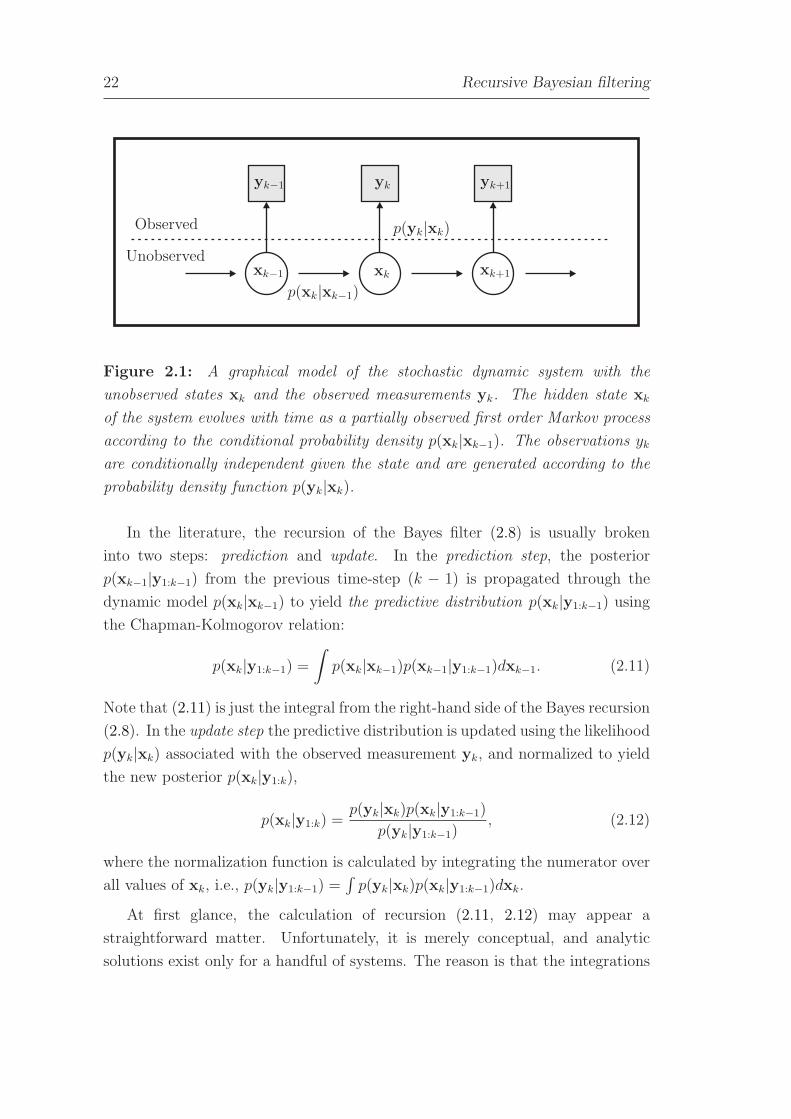
22 Recursive Bayesian filteringreplacemen

yk−1 yk yk+1

xk−1 xk xk+1

Observed

Unobserved

p(xk|xk−1)

p(yk|xk)

Figure 2.1: A graphical model of the stochastic dynamic system with the

unobserved states xk and the observed measurements yk. The hidden state xk

of the system evolves with time as a partially observed first order Markov process

according to the conditional probability density p(xk|xk−1). The observations yk

are conditionally independent given the state and are generated according to the

probability density function p(yk|xk).

In the literature, the recursion of the Bayes filter (2.8) is usually broken

into two steps: prediction and update. In the prediction step, the posterior

p(xk−1|y1:k−1) from the previous time-step (k − 1) is propagated through the

dynamic model p(xk|xk−1) to yield the predictive distribution p(xk|y1:k−1) using

the Chapman-Kolmogorov relation:

p(xk|y1:k−1) =

∫

p(xk|xk−1)p(xk−1|y1:k−1)dxk−1. (2.11)

Note that (2.11) is just the integral from the right-hand side of the Bayes recursion

(2.8). In the update step the predictive distribution is updated using the likelihood

p(yk|xk) associated with the observed measurement yk, and normalized to yield

the new posterior p(xk|y1:k),

p(xk|y1:k) =p(yk|xk)p(xk|y1:k−1)

p(yk|y1:k−1), (2.12)

where the normalization function is calculated by integrating the numerator over

all values of xk, i.e., p(yk|y1:k−1) =∫

p(yk|xk)p(xk|y1:k−1)dxk.

At first glance, the calculation of recursion (2.11, 2.12) may appear a

straightforward matter. Unfortunately, it is merely conceptual, and analytic

solutions exist only for a handful of systems. The reason is that the integrations

2.4 Historical approaches to recursive filtering 23

involved in calculating p(xk|y1:k−1) and p(yk|y1:k−1) generally do not have closed-

form solutions. Furthermore, even if the posterior p(xk|y1:k) can be found,

estimates of the target’s state, such as MMSE, are likely to be intractable [57]. A

number of approaches have been proposed in the literature to make the recursions

(2.11, 2.12) tractable. We give a brief overview of the better known ones next.

2.4 Historical approaches to recursive filtering

When the measurement and the system models are linear and the noise in both

models is Gaussian, closed-form solutions of the integrals in the recursions of the

Bayes filter exist. In particular, if we start from a Gaussian prior p(x0), and

assume that the prediction step (2.11) and the update step (2.12) of the recursive

Bayes filter are linear operations on Gaussians, then the resulting posterior is

a Gaussian as well. Thus the recursions (2.11, 2.12) can be interpreted as a

recursive estimation of the posterior’s p(xk|y1:k) mean and covariance. The filter

that emerges from this is the well-known Kalman filter [76], which was originally

derived by R. E. Kalman in the early sixties. Since then, it has been applied

extensively to various filtering problems and many variants have been presented;

see, e.g. [75, 133, 73, 67, 126].

In practice, the use of the Kalman filter is limited by the nonlinearity and

the non-Gaussian nature of the physical world. As an attempt to deal with

these nonlinearities, a modification called the extended Kalman filter (EKF) was

proposed (see, e.g. [67, 5]). This filter locally linearizes the system transition and

measurement models and then applies the standard Kalman filter to analytically

calculate the posterior p(xk|y1:k). Usually, a first-order Taylor series expansion is

used for the linearization. To obtain better approximations, higher-order variants

of EKF have been proposed [155]. However, the additional complexity, that these

higher-order extensions entail, has prevented their widespread use [6]. There

are two sources of inaccuracy in the EKF: The first is the linearization of the

system and measurement models, which is carried-out only at a single point

and does not take into account the uncertainty associated with that point. The

second problem is the assumption that the prior and posterior are Gaussians.

In fact, the nonlinearities in the models will result in posteriors being non-

Gaussian and sometimes even multi-modal after the propagation step. This

24 Recursive Bayesian filtering

undermines the Gaussian assumption in the EKF and consequently results in

degraded performance or even in complete failure of the tracker.

As an attempt to better deal with the nonlinearities of the measurement and

the system transition model, the so-called unscented Kalman filter (UKF) was

proposed by Julier and Uhllman [69, 71, 70, 72] in the late nineties. The basic

idea behind the UKF is to avoid the linearization of the measurement process and

system dynamics all together. The posterior is, like in EKF, still approximated

by a Gaussian, but this Gaussian is encoded through a set of points called sigma

points. These points are carefully chosen along the principal axes of the Gaussian

such that they can capture its covariance and the mean value. In the propagation

step, the points are propagated through the true nonlinear system and capture

the mean and the covariance of the new posterior accurately up to the third

order (in terms of Taylor expansion) [69]. This is a significant improvement in

comparison with the standard EKF, whose approximation is accurate only up to

the first order. Furthermore, the computational complexity of the UKF is lower

than that of the EKF, since it does not require linearization. Separately from the

UKF, another filter called the central-difference Kalman filter (CDKF) has been

proposed [79, 117]. Der Merwe [161, 159] observed that the UKF and CDKF

algorithms are related through an implicit use of a technique called weighted

statistical linear regression [94], which is responsible for determining the locations,

as well as the weights of the sigma points. Thus these filters have been given a

common name: sigma-point Kalman filters (SPKF) [159]. Although SKPF is

more accurate than EKF, it still assumes that the posterior can be approximated

by a single Gaussian. As such, it is still prone to failure in certain nonlinear,

non-Gaussian problems which involve multi-modal and/or heavy-tailed posterior

distributions.

As an alternative to approximating the posterior using only a single Gaussian,

a Gaussian sum filter (GSF) was proposed [150, 4], which applies a mixture

of Gaussians to better model the multimodality in the posterior distribution.

The motivation behind this was the fact that any non-Gaussian density can be

sufficiently well approximated by a sufficiently large number of Gaussians [165].

Thus the GSF was conceptually presented as a bank of extended Kalman filters,

where at each time-step, each component of the Gaussian mixture was propagated

using an EKF. One drawback of the filter was that the number of components in

the mixture had to be specified in advance. Another drawback was that in cases

2.4 Historical approaches to recursive filtering 25

where the observation noise and/or the system noise were also approximated by

a Gaussian mixture model, the number of components in the posterior increased

exponentially after each tracking iteration and methods for reducing the number

of components had to be used. Furthermore, since the GSF used EKF to

propagate the components of the mixture, it inherently suffered from the problem

of the first-order linearization in the EKF.

In contrast to the parametric models, which use Gaussians or Gaussian

mixtures to calculate the recursions in the Bayes filter analytically, non-

parametric methods, called grid-based methods, have been proposed to calculate

the recursions of the Bayes filter numerically. These approaches are based on

discretizing the continuous state-space into a predefined set of cells and then

evaluating the posterior only at these cells. In some variations, the posterior

is approximated using a discrete distribution over the grid cells [149]. Other

approaches use splines [27], step functions [86], or apply quadrature methods

[166]. The advantage of these approaches is that they simplify the recursions

of the Bayes filter, as each point on the grid is updated independently of the

others. Therefore, given enough cells, they hold a potential of approximating

fairly complex distributions. A significant drawback of the grid-based methods

is, however, that they require specifying the number of cells in advance, and the

grid has to be sufficiently dense to allow good approximation of the posterior.

With increasing dimension of the state-space, the computational burden then

increases dramatically. Another drawback is that, because the state of the target

is moving through the continuous state-space, the grid also has to move along

with the target, and has to scale accordingly to cover the significant probability-

mass corresponding to the target’s current state. This is a nontrivial task which

further increases the computational burden of the method.

In the late eighties and early nineties, with the advent of increased

computational power in computers, significant steps have been made toward

calculating the recursions in the Bayes recursive filter by means of simulation [83,

82]. As a result, a number of methods have been independently developed in

such fields as statistics, econometrics, engineering and computer science, that

were based on evaluating the integrals of the Bayesian recursion by Monte

Carlo sampling. These methods are commonly known as sequential Monte Carlo

methods or particle filters and are described next.

26 Recursive Bayesian filtering

2.5 Monte-Carlo-based recursive filtering

The aim of recursive Bayesian filtering is to calculate the posterior distribution

p(xk|y1:k) of the target’s state xk given some observations yk. Once the posterior

is known, various estimates of the target’s state can be calculated. For example,

the minimum-mean-squared-error (MMSE) estimate of the target state can be

obtained by taking the expectation 〈xk〉p(xk|y1:k). However, the MMSE estimate

involves solving a high-dimensional integral which is often intractable. A common

approach to evaluate intractable high-dimensional integrals is to apply Monte

Carlo integration, where the integrals are replaced by summations over discrete

sets of points. In this section we will first briefly overview the theoretical

background of Monte Carlo integration and show how it is used to approximate

the recursive Bayes filter. We will point out some drawbacks and implementation

issues of this approximation and discuss solutions and simplifications proposed in

the literature. In light of these, we will finally present a well-known approximate

recursive Bayes filter called the particle filter.

2.5.1 Perfect Monte Carlo sampling

First we will discuss how Monte Carlo methods can be conceptually used to

approximate integrals. For the sake of clarity we will drop the subscripts (·)k,

which indicate the time-steps, for now and reintroduce them later, when we

consider application of these methods to Bayesian filtering.

Note that in tracking we are generally interested in calculating expectations

over some posteriors p(x|y), which are integrals of type

I(f) =

∫

f(x)p(x|y)dx,

where f(·) is p(x|y)-integrable function of x. In a perfect Monte Carlo sampling,

the integral I(f) can be approximated as follows. First, N independent samples

x(i)i=1...N are drawn from the posterior p(x|y). Using these samples, the

posterior can be approximated by the following empirical estimate

pN(x|y) =1

N

N∑

i=1

δx(i)(x), (2.13)

which is essentially a set of Dirac-delta functions δx(i)(x) located at sampled points

x(i). Replacing p(x|y) with its empirical estimate pN(x|y), the integral I(f)

2.5 Monte-Carlo-based recursive filtering 27

(2.13) can now be numerically approximated with IN(f) using the Monte Carlo

integration

IN(f) =

∫

f(x)pN(x|y)dx

=1

N

N∑

i=1

∫

f(x)δx(i)(x)dx

=1

N

N∑

i=1

f(x(i)). (2.14)

The validity of the approximation I(f) ≈ IN(f) is guaranteed by the strong

law of large numbers ([43], page 7), which states that the average of many

independent random numbers with a common mean and finite variance converges

to the common mean

limN→∞

IN(f) = I(f), with probability one.

Moreover, if the variance σ2f of f(x) with respect to p(x|y) is finite, the central

limit theorem tells us that by increasing N , the difference between the integral

I(f) and its approximation IN(f) approaches a normal distribution with variance

σ2f , √

N [IN(f)− I(f)] =⇒N→∞

N (0, σ2f ), (2.15)

where ⇒ denotes convergence in distribution ([43], page 7). From (2.15) we see

that the accuracy of the estimator IN(f) increases with the number of samples

and does not depend directly on the dimension of the integrand3. In contrast,

in a deterministic numerical integration the accuracy of the integral decreases as

the dimension of the integrand increases ([43], page 7).

The above discussion tells us that if we are able to provide independent

samples from p(x|y), then the integrals of type (2.13) can be easily approximated.

In practice, however, p(x|y) will be multivariate, nonstandard and known only

up to a proportionality constant. Thus sampling from p(x|y) directly is usually

impossible and alternative solutions are required. One common solution is to use

importance sampling.

3Note, however, that σ2f in (2.15) may still grow appreciably with the dimension of the

integrand [57].

28 Recursive Bayesian filtering

2.5.2 Importance sampling

Let p(x|y) be some distribution which is difficult to sample from, but can be

evaluated up to a proportionality constant as

p(x|y) = Cpp(x|y). (2.16)

Let q(x|y) be another distribution which is easy to sample, can be also evaluated

point-wise, and has the same support as p(x|y)4. In the literature, q(x|y) is

usually called the importance function or the proposal distribution.

With the above definitions, the integral (2.13) can be rewritten

I(f) =

∫

f(x)p(x|y) =

∫

f(x)q(x|y)

q(x|y)

1

Cp

p(x|y)dx =1

Cp

∫

f(x)q(x|y)w(x)dx,

where p(x|y) was absorbed into

w(x) =p(x|y)

q(x|y). (2.17)

The proportionality constant Cp is obtained by integrating both sides of (2.16),

Cp =

∫

p(x|y)dx =

∫

q(x|y)w(x)dx,

and I(f) can be rewritten as

I(f) =1

∫

q(x|y)w(x)dx

∫

f(x)q(x|y)w(x)dx. (2.18)

Since q(x|y) can be easily sampled, it can be approximated by an empirical

Monte Carlo estimate (2.13)

qN(x|y) =1

N

N∑

i=1

δx(i)(x), (2.19)

where x(i)i=1:N is a set of independent and identically distributed (i.d.d.)

samples from q(x|y). The integral I(f) (2.18) can now be approximated by

IN(f), where

IN(f) =1

∫

qN(x|y)w(x)dx

∫

f(x)qN(x|y)w(x)dx

=1

1N

∑N

i=1 w(x(i))

1

N

∑N

i=1f(x(i))w(x(i)).

4We say that q(x|y) has the same support as p(x|y) when it is nonzero at least for all those

x, for which p(x|y) is nonzero as well.

2.5 Monte-Carlo-based recursive filtering 29

By cancelling the term 1N

in the above equation and taking the normalization

into the sum, we can further rewrite the integral as

IN(f) =∑N

i=1f(x(i))w(i) , w(i) =

w(x(i))∑N

i=1 w(x(i)). (2.20)

It is beneficial to note that, in terms of a perfect Monte Carlo sampling, the

integral IN(f) can be viewed as an expectation of f(x) under the following

empirical distribution

pN(x|y) =1

N

N∑

i=1

w(x(i))δx(i)(x). (2.21)

Since IN(f) from (2.20) is an equivalent of IN(f) from (2.13), pN(x|y) is

an empirical approximation to the reference distribution p(x|y). Therefore,

importance sampling can be viewed not only as means of approximating the

integrals of type (2.13), but actually as a methodology for generating empirical

distributions from a reference distribution without sampling it. The reference

distribution is thus approximated by a random measure, which is completely

specified by a set of N sample-weight pairs x(i), w(i)i=1:N . The latter are

commonly referred to as the particles.

Note that for a recursive Bayesian filtering, we require the probability density

functions to be calculated sequentially. In the following we show how this is

achieved by applying the above results from importance sampling.

2.5.3 Sequential importance sampling

In a general Bayesian filtering, we seek the posterior p(x0:k|y1:k) over a sequence of

states x0:k = x0, . . . ,xk of the target. From the results of importance sampling

we can approximate the posterior by an empirical distribution pN(x0:k|y1:k)

specified by N weighted particles x(i)0:k, w

(i)k i=1:N . Note that a particular sample

x(i)0:k in the i-th particle presents a trajectory through a target’s state-space and

is drawn with probability w(i) from the posterior. The posterior p(x0:k|y1:k) is in

general difficult to sample from and thus, in the spirit of importance sampling,

another distribution q(x0:k|y1:k) is defined from which samples can be drawn

easily. This new distribution, the proposal distribution, is further factored such

that it admits to a recursive form:

q(x0:k|y1:k) = q(xk|x0:k−1,y1:k)q(x0:k−1|y1:k−1).

30 Recursive Bayesian filtering

The i-th sample x(i)0:k can then be generated from the posterior p(x0:k|y1:k) by

choosing x(i)0:k−1 ∼ q(x

(i)0:k−1|y1:k), sampling a state x

(i)k ∼ q(xk|x(i)

0:k−1,y1:k) and

concatenating x(i)0:k = x(i)

k ,x(i)0:k−1. The corresponding weight, which makes x

(i)0:k

an equivalent sample from p(x0:k|y1:k), is then calculated according to (2.17)

w(i)k =

p(x(i)0:k|y1:k)

q(x(i)0:k|y1:k)

. (2.22)

From the recursive Bayes filter (2.4), with constraints (2.6, 2.7), the posterior

p(x(i)0:k|y1:k) is factored as5

p(x(i)0:k|y1:k) ∝ p(yk|x(i)

k )p(x(i)k |x

(i)k−1)p(x

(i)0:k−1|y1:k−1)

and the weight update equation (2.22) is rewritten as

w(i)k ∝

p(yk|x(i)k )p(x

(i)k |x

(i)k−1)

q(x(i)k |x

(i)0:k−1,y1:k)

p(x(i)0:k−1|y1:k−1)

q(x(i)0:k−1|y1:k−1)

. (2.23)

Since the second fraction on the right-hand side of (2.23) is just the i-th particle

weight from the previous time-step, we can further rewrite (2.23) as

w(i)k ∝ w

(i)k−1

p(yk|x(i)k )p(x

(i)k |xk−1)

q(x(i)k |x

(i)0:k−1,y1:k)

. (2.24)

Note that (2.29) is not a proper recursion, since the proposal distribution

is conditioned on y1:k, and thus requires storing the entire sequence of past

observations. To avoid that, the proposal is usually modified [6] into

q(x(i)k |x

(i)0:k−1,y1:k) = q(x

(i)k |x

(i)k−1,yk). (2.25)

From this definition of the importance function, the equation for calculating the

nonnormalized importance weights6 w(i)k takes the following form

w(i)k = w

(i)k−1

p(yk|x(i)k )p(x

(i)k |x

(i)k−1)

q(x(i)k |x

(i)k−1,yk)

, (2.26)

and the posterior p(xk|y1:k) in the current time-step is approximated by the

following random measure

pN(xk|y1:k) =1

N

N∑

i=1

w(i)k δ

x(i)k

(xk), (2.27)

5We have dropped the term p(yk|y1:k−1) from the denominator of the posterior since it is

independent from the sequence of the states x(i)0:k and is constant at k.

6By nonnormalized importance weights we refer to a set of weights which do not sum to

one.

2.5 Monte-Carlo-based recursive filtering 31

where w(i)k are now normalized importance weights, i.e., w

(i)k = w

(i)k (

∑N

i=1 w(i)k )−1.

An approximate recursive Bayesian filter that follows from (2.27) and (2.26) is

called the Sequential Importance Sampling (SIS) algorithm and is summarized in

Algorithm 2.1.

Input:

• Posterior from the previous time-step

p(xk−1|y1:k−1) ≈ x(i)k−1, w

(i)k−1Ni=1

Output:

• Posterior from the current time-step

p(xk|y1:k) ≈ x(i)k , w

(i)k Ni=1

1. For i = 1 : N ,

• Sample a new particle: x(i)k ∼ q(xk|x(i)

k−1,yk).

• Assign a weight: w(i)k = w

(i)k−1

p(yk|x(i)k

)p(x(i)k

|x(i)k−1)

q(x(i)k

|x(i)k−1,yk)

.

2. For i = 1 : N ,

• Normalize weights: w(i)k =

w(i)k

∑Nj=1 w

(j)k

.

3. The new random measure is an empirical approximation to the true posterior:

x(i)k , w

(i)k Ni=1 ≈ p(xk|y1:k).

Algorithm 2.1: Sequential Importance Sampling (SIS) algorithm.

2.5.4 Degeneracy of the SIS algorithm

The SIS algorithm has a major practical drawback. Since we are recursively

multiplying weights from the previous time-step with the weights in the current

time-step, the variances of weights tend to increase [43] with time and thus the

approximation of the posterior deteriorates. Furthermore, any estimate based on

this approximation (e.g., MMSE stimate) will deteriorate as well. Authors of [6]

have reported that in practice, after a few iterations, most of the normalized

32 Recursive Bayesian filtering

weights will be close to zero. From a computational standpoint this means that

most calculations are expended on calculating the weights whose contribution to

the estimates are negligible. This effect is in the literature commonly known as

the problem of degeneracy and is usually tackled by the following two approaches

[43, 6, 57]:

1. Choice of a suitable importance function.

2. Application of resampling.

Choice of the importance function

In view of alleviating the degeneracy of weights in SIS, the optimal choice

of the importance function is that which minimizes the variance of the true

weights, conditioned on the previous state and the current measurement [6].

It has been shown in [43] that in terms of variance minimization, the optimal

importance function is q(xk|xk−1,yk) = p(xk|xk−1,yk). There are two cases in

which such an importance function can be used [6]. One is when the state-

space of xk is discrete and finite. The other is when the measurement model

is linear and the noise in the system and measurement model is Gaussian.

Unfortunately, as we will see in later sections, these restrictions do not apply

for our applications of visual tracking. Various authors have proposed methods

that use other, suboptimal, importance functions. Among them are the auxiliary

particle filter [129], Gaussian mixture sigma-point particle filter [160], annealed

particle filter [41], partitioned sampling [107] and layered sampling [124], to name

but a few.

An alternative choice of the importance function is the prior transition model

q(xk|xk−1) = p(xk|xk−1). (2.28)

What is appealing about this choice is that it requires us to sample from the

system dynamic model, which is often easy. Furthermore, the weight update

equation (2.26) simplifies to

w(i)k = w

(i)k−1p(yk|xk). (2.29)

However, choosing the prior for the importance function may also have a

deteriorative effect on the performance of SIS. This happens in situations when

2.5 Monte-Carlo-based recursive filtering 33

the likelihood p(yk|xk) is quite peaked in comparison to the prior p(xk|xk−1).

An example of such a situation is illustrated in Figure 2.2. Only a few particles

generated from the prior are located at the peak of the likelihood function. As

a result, majority of the particles have a weight very close zero. Note that this

is in fact equivalent to the problem of degeneracy which we are trying to avoid.

Nevertheless, the simplicity of implementation, and weight calculation that such

a choice of importance function offers, makes it a very popular choice among

practitioners.

p(yk|xk)

p(xk|x(i)k−1)

xk

Figure 2.2: Samples (depicted by circles) are drawn from the prior p(xk|x(i)k−1).

A weight is assigned to each sample according to the likelihood function p(yk|xk).

The weight of each sample is indicated by the radius of the circle; a large radius

corresponds to a large weight, while a small radius corresponds to a low weight.

Note that since only a few samples are generated at the peak of the likelihood

function, the majority of samples have weights close to zero.

Application of resampling

The second approach to alleviating the effects of degeneracy is to use resampling

whenever a significant degeneracy is observed. Recall that the posterior p(xk|y1:k)

is approximated by the following random measure

pN(xk|y1:k) =∑N

i=1w

(i)k δ

x(i)k

(xk).

Resampling can then be thought of as generating N new samples from pN(xk|y1:k)

and is described by a mapping

x(i)k , w

(i)k Ni=1 → x(i)

k ,1

NNi=1 , Pr(x

(i)k = x

(i)k ) = w

(i)k , (2.30)

34 Recursive Bayesian filtering

under which all new particles x(i)k have equal weights 1

Nand are still approximately

distributed according to the original posterior p(xk|y1:k). In other words,

resampling avoids degeneracy of weights by generating a new random measure

pN(xk|y1:k) =∑N

i=1

1

Nδx

(i)k

(xk)

by selecting the particles with high weights multiple times and discarding

those with smaller weights. Therefore, the particles are herded in regions of

high probability density of the posterior p(xk|y1:k). Resampling is required

especially in those situations, when the particle set becomes degenerated. In

the literature [101, 13, 6], an effective sample size Neff , sometimes also called the

survival diagnostic [106], is proposed as a measure of degeneracy

Neff =1

∑N

i=1 (w(i)t )2

. (2.31)

Therefore, when Neff falls below a predefined threshold, the particle set is

resampled. Many resampling schemes have been proposed in the literature:

stratified sampling and residual sampling [101], systematic resampling [83],

deterministic resampling [106], resampling based on ordered statistics [134, 31],

residual sampling [101], regularized sampling [47], etc. We use a deterministic

resampling [106] in our implementation, since it is simple to implement and the

complexity of the algorithm is O(N). The deterministic resampling is summarized

in Algorithm 2.2.

It is important to note that while resampling does alleviate the problem

of degeneracy it introduces other problems. One is that particles with higher

weights are chosen multiple times in the resampling step. This can reduce the

diversification of the particles, since the new particle-set contains multiple copies

of the same particles. This is known in the literature as sample impoverishment

and can be critical especially when the system noise is small [6]. In those

situations, after a few iterations, the entire particle set will collapse into a single

point [6]. Nevertheless, despite the drawback of possible sample impoverishment,

resampling deals well with the problem of degeneracy and has as such become an

integral part of all modern particle-set-based recursive Bayesian filters.

2.5.5 Particle filters

If resampling (e.g., Algorithm 2.2) is used with the SIS algorithm (Algorithm 2.1)

and the effective sample size Neff (2.31) is used to decide when to resample, we

2.5 Monte-Carlo-based recursive filtering 35

Input:

• Posterior p(xk|y1:k) ≈ x(i)k , w

(i)k Ni=1

Output:

• Resampled posterior p(xk|y1:k) ≈ x(i)k , 1

NNi=1

1. Generate a cumulative distribution c(i)Ni=1 from the particle weights

• c(i) =∑i

j=1 w(j)k .

2. Initialize: l = 1

3. For i = 1 : N ,

• while ( iN

> c(l)) : l + +.

• choose x(i)k = x

(l)k and set w

(i)k = 1

N.

Algorithm 2.2: Deterministic resampling.

obtain the so-called generic particle filter, which is summarized in Algorithm 2.3.

A special variant of the generic particle filter has become popular and widely

used for visual target tracking in the last decade. This variant assumes the

following two simplifications:

• The prior is used in the importance function:

q(xk|xk−1,yk) = p(xk|xk−1).

• Resampling is executed at each iteration (this is equivalent to setting

Nthres =∞ in the Algorithm (2.3).

The variant that uses the above two simplifications has emerged under various

names like the bootstrap particle filter (BPF) [53] (published in 1993) and the

Condensation algorithm [63] (published in 1996) to name just the more visible

36 Recursive Bayesian filtering

Input:

• Posterior from the previous time-step

p(xk−1|y1:k−1) ≈ x(i)k−1, w

(i)k−1Ni=1

Output:

• Posterior from the current time-step

p(xk|y1:k) ≈ x(i)k , w

(i)k Ni=1

1. Evaluate Neff using (2.31).

2. If Neff > Nthres

Resample x(i)k−1, w

(i)k−1Ni=1 using Algorithm 2.2.

• x(i)k−1, w

(i)k−1Ni=1 → x

(i)k−1,

1NNi=1

3. For i = 1 : N ,

• Sample a new particle x(i)k ∼ q(xk|x(i)

k−1,yk)

• Assign a new weight w(i)k =

p(yk|x(i)k

)p(x(i)k

|x(i)k−1)

q(x(i)k

|x(i)k−1,yk)

4. For i = 1 : N ,

• Normalize the weights: w(i)k =

w(i)k

∑Nj=1 w

(j)k

5. The new random measure is an empirical approximation to the posterior:

x(i)k , w

(i)k Ni=1 ≈ p(xk|y1:k)

Algorithm 2.3: A generic particle filter.

two. The bootstrap particle filter is summarized in Algorithm 2.4. Note that

since the particle filter approximates the posterior over the target’s state by a

weighted sample-set, p(xk|y1:k) ≈ x(i)k , w

(i)k Ni=1, the minimum-mean-squared-

error (MMSE) estimate xk is approximated as

xk =N

∑

i=1

x(i)k w

(i)k . (2.32)

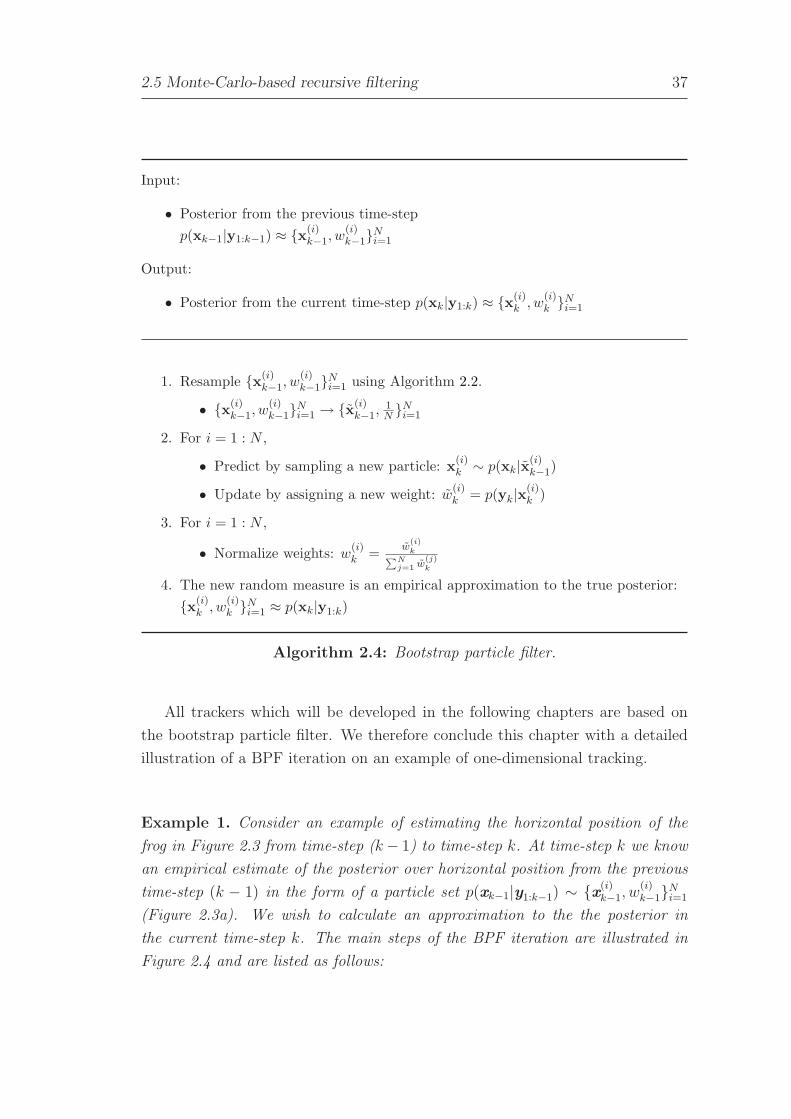
2.5 Monte-Carlo-based recursive filtering 37

Input:

• Posterior from the previous time-step

p(xk−1|y1:k−1) ≈ x(i)k−1, w

(i)k−1Ni=1

Output:

• Posterior from the current time-step p(xk|y1:k) ≈ x(i)k , w

(i)k Ni=1

1. Resample x(i)k−1, w

(i)k−1Ni=1 using Algorithm 2.2.

• x(i)k−1, w

(i)k−1Ni=1 → x

(i)k−1,

1NNi=1

2. For i = 1 : N ,

• Predict by sampling a new particle: x(i)k ∼ p(xk|x(i)

k−1)

• Update by assigning a new weight: w(i)k = p(yk|x(i)

k )

3. For i = 1 : N ,

• Normalize weights: w(i)k =

w(i)k

∑Nj=1 w

(j)k

4. The new random measure is an empirical approximation to the true posterior:

x(i)k , w

(i)k Ni=1 ≈ p(xk|y1:k)

Algorithm 2.4: Bootstrap particle filter.

All trackers which will be developed in the following chapters are based on

the bootstrap particle filter. We therefore conclude this chapter with a detailed

illustration of a BPF iteration on an example of one-dimensional tracking.

Example 1. Consider an example of estimating the horizontal position of the

frog in Figure 2.3 from time-step (k− 1) to time-step k. At time-step k we know

an empirical estimate of the posterior over horizontal position from the previous

time-step (k − 1) in the form of a particle set p(xk−1|y1:k−1) ∼ x(i)k−1, w

(i)k−1Ni=1

(Figure 2.3a). We wish to calculate an approximation to the the posterior in

the current time-step k. The main steps of the BPF iteration are illustrated in

Figure 2.4 and are listed as follows:

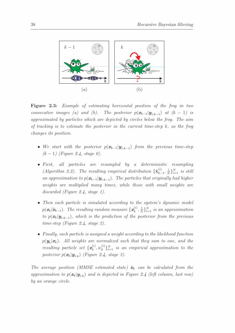
38 Recursive Bayesian filtering

x

k − 1

x

k

(a) (b)

Figure 2.3: Example of estimating horizontal position of the frog in two

consecutive images (a) and (b). The posterior p(xk−1|y1:k−1) at (k − 1) is

approximated by particles which are depicted by circles below the frog. The aim

of tracking is to estimate the posterior in the current time-step k, as the frog

changes its position.

• We start with the posterior p(xk−1|y1:k−1) from the previous time-step

(k − 1) (Figure 2.4, stage 0).

• First, all particles are resampled by a deterministic resampling

(Algorithm 2.2). The resulting empirical distribution x(i)k−1,

1NNi=1 is still

an approximation to p(xk−1|y1:k−1). The particles that originally had higher

weights are multiplied many times, while those with small weights are

discarded (Figure 2.4, stage 1).

• Then each particle is simulated according to the system’s dynamic model

p(xk|xk−1). The resulting random measure x(i)k , 1

NNi=1 is an approximation

to p(xk|y1:k−1), which is the prediction of the posterior from the previous

time-step (Figure 2.4, stage 2).

• Finally, each particle is assigned a weight according to the likelihood function

p(yk|xk). All weights are normalized such that they sum to one, and the

resulting particle set x(i)k , w

(i)k Ni=1 is an empirical approximation to the

posterior p(xk|y1:k) (Figure 2.4, stage 3).

The average position (MMSE estimated state) xk can be calculated from the

approximation to p(xk|y1:k) and is depicted in Figure 2.4 (left column, last row)

by an orange circle.

2.5 Monte-Carlo-based recursive filtering 39

stage 0

stage 1

stage 2

stage 3

k

k

k

k

k − 1

x(i)k−1, w

(i)k−1 ≈ p(xk−1|y1:k−1)

xk

xk

xk

xk

xk

x(i)k−1, 1

N ≈ p(xk−1|y1:k−1)

x(i)k

, 1N ≈ p(xk|y1:k−1)

x(i)k

, w(i)k

≈ p(xk|y1:k)

Posterior at (k − 1): p(xk−1|y1:k−1)

Posterior at k: p(xk|y1:k)

Simulation with dynamic model p(xk|xk−1)

Assign weights according to p(yk|xk)

Deterministic resampling

Figure 2.4: An illustration of a single iteration of the bootstrap particle filter

(Algorithm 2.4) with four stages from Example 1. The posterior over the frog’s

horizontal position (stage 0) is presented by twelve particles, where each particle

is depicted by a purple circle and the weight of the particle is indicated by the

circle’s radius: the larger the radius, the larger the weight. The three subsequent

stages are resampling (stage 1), prediction (stage 2) and update (stage 3). The

left column shows how particles evolve with respect to the frog’s position, while the

right column shows different stages in more detail. The average state (position)

of the frog in the current time-step is depicted by an orange circle overlaid on the

particles in the left column of stage 3.

40 Recursive Bayesian filtering

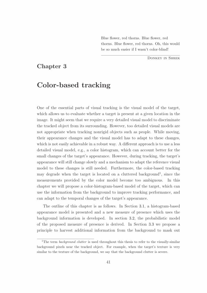
Blue flower, red thorns. Blue flower, red

thorns. Blue flower, red thorns. Oh, this would

be so much easier if I wasn’t color-blind!

Donkey in Shrek

Chapter 3

Color-based tracking

One of the essential parts of visual tracking is the visual model of the target,

which allows us to evaluate whether a target is present at a given location in the

image. It might seem that we require a very detailed visual model to discriminate

the tracked object from its surrounding. However, too detailed visual models are

not appropriate when tracking nonrigid objects such as people. While moving,

their appearance changes and the visual model has to adapt to these changes,

which is not easily achievable in a robust way. A different approach is to use a less

detailed visual model, e.g., a color histogram, which can account better for the

small changes of the target’s appearance. However, during tracking, the target’s

appearance will still change slowly and a mechanism to adapt the reference visual

model to these changes is still needed. Furthermore, the color-based tracking

may degrade when the target is located on a cluttered background1, since the

measurements provided by the color model become too ambiguous. In this

chapter we will propose a color-histogram-based model of the target, which can

use the information from the background to improve tracking performance, and

can adapt to the temporal changes of the target’s appearance.

The outline of this chapter is as follows. In Section 3.1, a histogram-based

appearance model is presented and a new measure of presence which uses the

background information is developed. In section 3.2, the probabilistic model

of the proposed measure of presence is derived. In Section 3.3 we propose a

principle to harvest additional information from the background to mask out

1The term background clutter is used throughout this thesis to refer to the visually-similar

background pixels near the tracked object. For example, when the target’s texture is very

similar to the texture of the background, we say that the background clutter is severe.

41

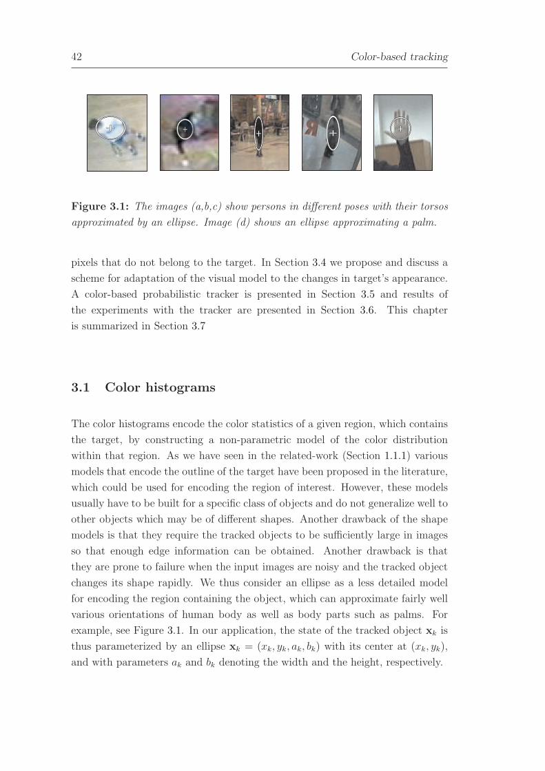
42 Color-based tracking

Figure 3.1: The images (a,b,c) show persons in different poses with their torsos

approximated by an ellipse. Image (d) shows an ellipse approximating a palm.

pixels that do not belong to the target. In Section 3.4 we propose and discuss a

scheme for adaptation of the visual model to the changes in target’s appearance.

A color-based probabilistic tracker is presented in Section 3.5 and results of

the experiments with the tracker are presented in Section 3.6. This chapter

is summarized in Section 3.7

3.1 Color histograms

The color histograms encode the color statistics of a given region, which contains

the target, by constructing a non-parametric model of the color distribution

within that region. As we have seen in the related-work (Section 1.1.1) various

models that encode the outline of the target have been proposed in the literature,

which could be used for encoding the region of interest. However, these models

usually have to be built for a specific class of objects and do not generalize well to

other objects which may be of different shapes. Another drawback of the shape

models is that they require the tracked objects to be sufficiently large in images

so that enough edge information can be obtained. Another drawback is that

they are prone to failure when the input images are noisy and the tracked object

changes its shape rapidly. We thus consider an ellipse as a less detailed model

for encoding the region containing the object, which can approximate fairly well

various orientations of human body as well as body parts such as palms. For

example, see Figure 3.1. In our application, the state of the tracked object xk is

thus parameterized by an ellipse xk = (xk, yk, ak, bk) with its center at (xk, yk),

and with parameters ak and bk denoting the width and the height, respectively.

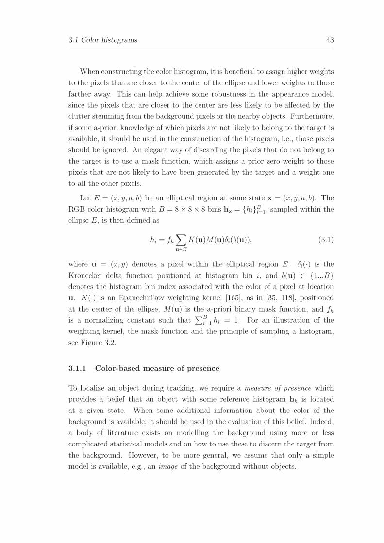
3.1 Color histograms 43

When constructing the color histogram, it is beneficial to assign higher weights

to the pixels that are closer to the center of the ellipse and lower weights to those

farther away. This can help achieve some robustness in the appearance model,

since the pixels that are closer to the center are less likely to be affected by the

clutter stemming from the background pixels or the nearby objects. Furthermore,

if some a-priori knowledge of which pixels are not likely to belong to the target is

available, it should be used in the construction of the histogram, i.e., those pixels

should be ignored. An elegant way of discarding the pixels that do not belong to

the target is to use a mask function, which assigns a prior zero weight to those

pixels that are not likely to have been generated by the target and a weight one

to all the other pixels.

Let E = (x, y, a, b) be an elliptical region at some state x = (x, y, a, b). The

RGB color histogram with B = 8× 8× 8 bins hx = hiBi=1, sampled within the

ellipse E, is then defined as

hi = fh

∑

u∈E

K(u)M(u)δi(b(u)), (3.1)

where u = (x, y) denotes a pixel within the elliptical region E. δi(·) is the

Kronecker delta function positioned at histogram bin i, and b(u) ∈ 1...Bdenotes the histogram bin index associated with the color of a pixel at location

u. K(·) is an Epanechnikov weighting kernel [165], as in [35, 118], positioned

at the center of the ellipse, M(u) is the a-priori binary mask function, and fh

is a normalizing constant such that∑B

i=1 hi = 1. For an illustration of the

weighting kernel, the mask function and the principle of sampling a histogram,

see Figure 3.2.

3.1.1 Color-based measure of presence

To localize an object during tracking, we require a measure of presence which

provides a belief that an object with some reference histogram hk is located

at a given state. When some additional information about the color of the

background is available, it should be used in the evaluation of this belief. Indeed,

a body of literature exists on modelling the background using more or less

complicated statistical models and on how to use these to discern the target from

the background. However, to be more general, we assume that only a simple

model is available, e.g., an image of the background without objects.

44 Color-based tracking

E = x, y, a, b

E

u(x, y)

K(u)

(a) (b)

(c) (d)

Figure 3.2: The target’s state is modelled as an elliptical region (a). The

weighting kernel and its parameters are sketched in (b). The mask function

which masks out the background pixels is shown in (c). The target histogram

is sampled by considering only pixels which are visible through the mask function

and assigning a weight to each pixel according to the weighting kernel (d).

We thus define the measure of the presence which evaluates whether a target

with a predefined reference histogram hk is present at some state xk as

D(hA,hk;hB) = β−1ρ(hA,hk;hB), (3.2)

where hA and hB are histograms sampled at the state xk on the current and the

precalculated background image, respectively. β is the ratio between the number

of pixels within the elliptical region of xk that are assigned to the foreground by

the mask function M(u) and the number of those assigned to the background.

ρ(hA,hk;hB) is the normalized distance between hA and hk, given the background

histogram hB, defined as

ρ(hA,ht;hB) =(hA,hk)

√

(hB,hk)2 + (hA,hk)2, (3.3)

where (h1,h2) = 1 − ∑

i

√h1ih2i is the Hellinger distance [11, 137, 154].

Note that the Hellinger distance is related to the well-known Bhattacharryya

coefficient [74], it is a metric and has a geometrical interpretation. For a detailed

discussion on this distance please see [11, 154].

3.2 The likelihood function 45

(a) (b) (c)

Figure 3.3: The histogram of a basketball player was sampled within the ellipse

(a). A non-normalized distance (hA,ht) calculated at different positions around

the player is shown in (b). The result for the proposed normalized distance

measure ρ(hA,ht;hB) is shown in (c). For better visualization, one minus the

distance measures are shown. The correct position of the player is depicted by

a white arrow and a circle in each image. Notice how the mode corresponding

to the selected player is more pronounced with respect to the background clutter

when the normalized distance is used (c).

The normalization term in (3.3) incorporates the distance between the

reference color model and the background color. Such a normalization aids

tracking when the target’s color is similar to the background. In these situations

the measure (3.3) favors those regions for which the reference color model is closer

to the color in the current image than to the background color. In practice, when

using a particle filter, this effectively attenuates the background clutter and forces

particles closer to the target. An example of the normalized and non-normalized

distance measure is shown in Fig. 3.3.

3.2 The likelihood function

To carry out the update step of the particle filter, e.g., (Algorithm 2.4), we require

the probability density function (pdf) of the presence measure (3.2). Due to the

lack of a rigorous physical background with which the analytical form of this pdf

could be derived, an experimental approach was chosen instead.

The pdf of (3.2) was estimated from a large number of examples of moving

persons; see Fig. 3.4a for examples. Some of these persons were tracked using a

46 Color-based tracking

D(hA,ht;hB)

(a) (b)

Figure 3.4: The left-hand image shows examples of persons which were used

to estimate the empirical probability density function of the measure (3.2). The

right-hand image shows this function in the form of a histogram, and overlaid is

the maximum-likelihood fitted gamma probability density function.

simple tracker from the literature [118]. In cases when the simple tracker failed,

we have resorted to manual marking. This enabled us to obtain approximately

115,000 values of the measure (3.2), which are visualized by the histogram in

Fig. 3.4b.

To identify the best model for the gathered data, a model selection was carried

out using the Akaike information criterion (AIC) [3] among four models of the

probability density functions: exponential, gamma, inverse gamma and zero-mean

Gaussian2. The test with the AIC showed that the gamma function explained the

data significantly better than the other functions. For this reason the probability

density function of measure (3.2) was chosen in the form of

p(yt|xt) ∝ D(hA,ht;hB)γ1−1e−D(hA,ht;hB)

γ2 . (3.4)

The parameters γ1 and γ2 were estimated from the data using the maximum-

likelihood approach. The estimated values were γ1 = 1.769 and γ2 = 0.066. For

more details on the model selection results, please see the Appendix A.

2Only the main results of the model selection using Akaike information criterion are reported

here and the reader is referred to Appendix A for more details.

3.3 The background mask function 47

Note that the gamma distribution assigns small probability values to those

values of the measure (3.2) that are very close to zero. At first glance this may not

seem reasonable for the purposes of object localization; however, if we observe a

moving nonrigid object such as a person in two consecutive time-steps, it is more

likely that the person’s appearance will change within these two time-steps than

stay the same. This is an inherent property of the visual dynamics of nonrigid

objects and is implicitly captured by the likelihood function (3.4).

3.3 The background mask function

While color histograms are powerful color cues for tracking textured objects,

they can fail when the object is moving on a similarly textured background.

This is usually due to their inability to capture the spatial relations in the

texture, and the fact that they are always sub-sampled in order to increase their

robustness. There is, however, still some useful information left in the current

and the background image – the difference between the two. By thresholding this

difference image with some appropriate threshold κk, we can construct a mask

image that filters out those pixels which are likely to belong to the background.

Since, in general, the illumination of the observed scene is non-uniform in space

and time, the threshold has to be estimated dynamically for the tracked object.

We base our method for mask generation on the following observation. When

an object described by an ellipse is located on the visually-similar background,

some small portion of the pixels within the ellipse come either from the

background, or come from the object but are very similar to the background.

We thus assume that in those situations we can assign some percentage η0 of the

pixels within the object’s ellipse to the background.

Let xk denote the estimated state of the target at time-step k. Let hA and

hB be the histograms sampled at that state on the current image A(·) and the

background image B(·), respectively. The current mask function is defined as

MD(u) =

1 ; ‖A(u)−B(u)‖ ≥ κk

0 ; otherwise, (3.5)

where u is some pixel, ‖ · ‖ is the L2 norm and κk is the threshold in the current

time-step.

48 Color-based tracking

Note that we have to generate the mask function only when the tracked object

is similar enough to the background. Thus in practice we verify after each tracking

iteration the similarity between the target’s visual model and the background. If

this similarity is within a predefined bound ((hA,hB) < thresh), then the mask

is generated in the next time-step. The threshold κk+1 for the next time-step is

estimated as the threshold that would in the current time-step produce a mask

function such that a predefined percentage η0 of the pixels within the ellipse of the

current state xk would be assigned to the background. Otherwise, if (hA,hB) ≥thresh, the mask is not generated in the next time-step and MD(u) = 1 in (3.5)

for all pixels u.

3.3.1 Implementation of dynamic threshold estimation

The procedure for calculating the appropriate κk+1 is as follows. Let

dE = diEmD

i=1 be a set of pixel-wise intensity differences between the current

image A(·) and the background image B(·) calculated within the ellipse E of the

estimated state xk and let these differences be ordered in an ascending order. We

define the cumulative function corresponding to the ordered differences as

clE =l

∑

j=0

1

mD

, (3.6)

and then the smallest l at which c(l+1)E exceeds η0 is the required threshold

κt+1 = κt(η0), or formally,

κt(η0) = dlE ; clE < η0 ≤ c(l+1)E. (3.7)

The parameters η0 and thresh were estimated empirically by manually

selecting persons as they moved on a heavily cluttered background. We have

observed that usually when a person is located on a cluttered background, at least

25 percent of pixels within the ellipse describing that person can be assigned to

the background and thus we have chosen η0 = 25%. The parameter which decides

when to generate the mask was set in a similar empirical manner, and was set to

thresh = 0.8. The procedure of threshold approximation is illustrated with the

Example 2.

Example 2. Consider a situation where we observe a yellow person on a yellow

background (Figure 3.5a). Assume that at time-step k − 1 we know the state of

3.4 Adaptation of the visual model 49

that person described by the ellipse E (Figure 3.5a) and the background image

is available (Figure 3.5b). We want to determine a threshold κk(η0) such that

25 percent of pixels within the ellipse will be masked out by the resulting mask

function. We thus first calculate the ordered set of intensity differences between

the current image and the background within ellipse E in form of a histogram

of differences (Figure 3.5c). The corresponding cumulative function is shown in

Figure 3.5d. From the cumulative function we read off the difference value at

which the function exceeds η0 = 0.25 and we have κk(0.25) = 55. For illustration,

the mask function calculated from the current image and the background image is

shown in Figure 3.5e and the masked image of the person is shown in Figure 3.5f.

3.4 Adaptation of the visual model

When a nonrigid object such as a human body moves through an observed scene,

its texture varies due to the non-uniform lighting conditions, influences of the

background, and variations of the person’s pose. Therefore, the color model, i.e.,

the person’s current reference histogram hk, has to be able to adapt to these

changes. In addition, if the current state of the tracked person is likely to have

been falsely estimated, and the corresponding ellipse does not fully contain the

person, then the reference histogram should be updated by a very small amount,

or not at all. Otherwise, it should be adapted by some larger amount.

Let xk be the estimated state of a person at the current time-step. The

histograms hA and hB are sampled at that state on the current and the

background image, respectively. The adaptation equation then follows a simple

auto-regressive form

hk = αkhA + (1− αk)hk−1, (3.8)

where hk−1 is the reference histogram from the previous time-step. The intensity

of the adaptation is defined with respect to the normalized distance (3.3) between

hA and hk−1 as

αk = Ωmax · (1.0− ρ(hA,hk−1;hB)), (3.9)

where Ωmax denotes the maximal adaptation. In all experiments in this thesis

we use Ωmax = 0.05. This means, that, at each time-step, we allow at most 5%

adaptation of the reference histogram. The following example was designed to

50 Color-based tracking

E

At(·)E

B(·)

(a) (b)

dlE

n

dlE

(c) (d)

MD(·) A⊗MD

(e) (f)

Figure 3.5: Example of estimating the threshold κk at η0 = 0.25. A person

denoted by an ellipse is shown in (a) and the background image is shown in (b).

The histogram of intensity differences is shown in (c) and the resulting cumulative

function is shown in (d). The threshold corresponding to η0 = 0.25 is found at

dlE = 55 in (b). The resulting mask function is shown in (e), and (f) shows the

mask function superimposed over (a).

3.4 Adaptation of the visual model 51

provide some insight into the choice of maximal adaptation value. For better

illustration we will assume that the parameter αk is constant and equal to the

maximal adaptation, i.e., αk = 0.05.

Example 3. Assume we observe a controlled environment with a single object

illuminated by a white light. At time-step k = 0 we record its reference histogram

h0 and then turn on color lights such that the apparent color of the object changes.

The new color histogram of the object is hC and remains constant for all k > 0.

The model hk begins to adapt to the new histogram hC according to (3.8)

hk = (1− αk)hk−1 + αkhC .

Since we assume that αk and hC are constant, we can rewrite the reference

histogram at time-step k as

hk = (1− αk)kh0 + (1− (1− αk)

k)hC . (3.10)

Now say we want to know what portion of the new histogram hC has been

incorporated into the current reference histogram hk after 25th time-step3 at a

constant adaptation value αk = 0.05. Using (3.10) we have

h25 = (1− 0.05)25h0 + (1− (1− 0.05)25)hC

≈ 0.28h0 + 0.72hC ,

which means that after 25 time-steps the reference histogram hk contains

approximately one quarter of the reference histogram at k = 0, h0, and three

quarters of the new histogram hC.

A further insight into the influence of different values of αk is provided in

Figure 3.6(a). The graph shows the percentage of the histogram hC in hk after

25th time-step for different values of αk. We see that by setting αk = 0.2, the

reference histogram becomes practically equal to the current histogram after 25th

time-step. This means that at αk = 0.2, and at frame rate of 25 frames per second,

the reference histogram completely adapts to the instant change within the time-

span of one second. Figure 3.6(b) shows percentage of the new histogram in hk at

a constant adaptation αk = 0.05 with respect to time. We see that the reference

histogram would completely adapt to an instant change of person’s appearance

within 120 time-steps, which, at frame rate of 25 frames per second, amounts to

5 seconds.3Note that, in most of our experiments reported in this thesis, 25 frames corresponds to one

second of video.

52 Color-based tracking

Per

centa

ge

ofth

enew

his

togra

m

α

Per

centa

ge

ofth

enew

his

togra

m

Number of observed images

(a) (b)

Figure 3.6: Percentage of the new histogram in the reference histogram after 25

time-steps with respect to constant adaptation parameter α (a). Percentage of the

new histogram in the reference histogram at α = 0.05 with respect to number of

time-steps is shown in (b).

3.5 Color-based probabilistic tracker

In the previous sections we have presented an adaptive color-histogram-based

visual model of the target, which is able to harvest information about the color

of the background with the aim to better discriminate the target from the

background. In this section we show how the proposed color model can be used

for tracking within the framework of particle filters.

Prior to tracking, we first calculate the background image. This can be

achieved for example, either by taking a single image of an empty scene, or to

record a sequence of images and then construct a median image pixel-wise along

the temporal component. The tracker is initialized by selecting the target and

recording the reference histogram. This can be done, for example, by manually

clicking the target. Then at each tracking iteration the following steps are

executed. First, a mask function is calculated using the dynamically estimated

threshold from the previous time-step, as discussed in Section 3.3. Then an

iteration of the bootstrap particle filter (Algorithm 2.4) is executed using the

likelihood function derived in Section 3.2. The current estimate xk of the target

state (position and size of the ellipse) is calculated as a MMSE estimate (2.32).

A histogram is then sampled at the estimated state xk and used to adapt the

3.5 Color-based probabilistic tracker 53

reference histogram according to Section 3.4. Finally, in the last step of tracking

iteration, the threshold for generating the mask image in the next time-step is

calculated if necessary according to Section 3.3. This procedure is summarized

in Algorithm 3.1.

Initialize:

• Calculate the background image, e.g., pixel-wise by means of a median filter

along temporal axis.

• Initialize the tracker by selecting the target (e.g., manually).

Tracking:

1. For i = 1 : N ,

• Calculate the mask function according to Section 3.3.

• Execute an iteration of the bootstrap particle filter (Algorithm 2.4) using

the likelihood function from Section 3.4.

• Estimate the current state xt by MMSE estimate (2.32) from the particle

filter.

• Sample the histogram at xt and adapt the model to that histogram as in

Section 3.4.

• If required, estimate the threshold for the mask function MD(u) in the next

time-step (Section 3.3).

Algorithm 3.1: Color-based probabilistic tracker.

Note that the proposed color model and the probabilistic tracker in

Algorithm 3.1 require us to set some parameters. These are: the parameters of

the likelihood function, dynamic background subtraction and the parameters for

adaptation of the reference histogram. In the previous sections, we have discussed

how these parameters have been selected, and in all the following experiments in

this thesis their values are kept constant. For a better overview, we summarize

them in Table 3.1.

54 Color-based tracking

Table 3.1: Parameters of the color-based probabilistic tracker.

Parameters of the color-based likelihood function (3.4)

• (γ1, γ2) = (1.769, 0.066)

Parameters for dynamic background subtraction (Section 3.3.1)

• (η0, ρthresh) = (0.25, 0.8)

Maximal adaptation of the color model (3.9)

• Ωmax = 0.05

3.6 Experiments

A set of experiments was performed to evaluate how the proposed likelihood

function (Sect. 3.2), the adaptation scheme (Sect. 3.4) and the dynamic

background subtraction (Sect. 3.3) influence the performance of tracking persons

in images. In these experiments we have compared the proposed color-based

tracker from Algorithm 3.1, we denote it by Tcol, to a reference tracker Tref

from the literature [118]. The reference tracker Tref was also a color-histogram-

based particle filter, however, Tref did not account for the background in the

likelihood function and the adaptation, and did not use the dynamic background

subtraction scheme. Both trackers used 50 particles in the particle filter. The

target motion was modelled by two independent nearly-constant-velocity (NCV)

models in the horizontal and vertical direction. The dynamics of the target’s

size was modelled by two independent random-walk (RW) models in horizontal

and vertical direction. For a detailed description of the NCV and RW models,

and assumptions they enforce on dynamics, see Appendix B.1 and Appendix B.2,

respectively. The parameters of the NCV models were set for each set of the

experiments separately according to the expected size of the tracked object in

video. The parameters of the RW models were set such that the target’s size

would change approximately at most by 15 percent in between consecutive time-

steps.

Three experiments were considered for comparing performance of Tcol and

Tref . The first experiment considered tracking a person in a heavily cluttered

environment from a bird’s-eye view. The second experiment considered tracking

a person from a side-view in a less cluttered environment, in a situation where

that person is occluded by another, visually similar, person. The last, the third,

experiment considered tracking a person from a side-view moving camera. In

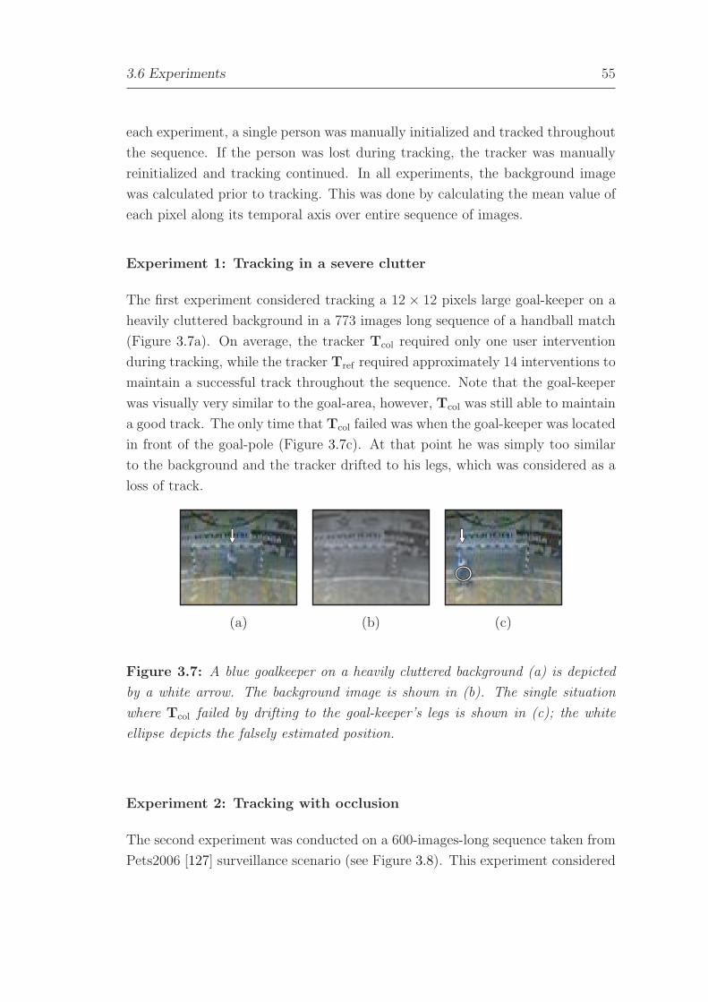
3.6 Experiments 55

each experiment, a single person was manually initialized and tracked throughout

the sequence. If the person was lost during tracking, the tracker was manually

reinitialized and tracking continued. In all experiments, the background image

was calculated prior to tracking. This was done by calculating the mean value of

each pixel along its temporal axis over entire sequence of images.

Experiment 1: Tracking in a severe clutter

The first experiment considered tracking a 12× 12 pixels large goal-keeper on a

heavily cluttered background in a 773 images long sequence of a handball match

(Figure 3.7a). On average, the tracker Tcol required only one user intervention

during tracking, while the tracker Tref required approximately 14 interventions to

maintain a successful track throughout the sequence. Note that the goal-keeper

was visually very similar to the goal-area, however, Tcol was still able to maintain

a good track. The only time that Tcol failed was when the goal-keeper was located

in front of the goal-pole (Figure 3.7c). At that point he was simply too similar

to the background and the tracker drifted to his legs, which was considered as a

loss of track.

(a) (b) (c)

Figure 3.7: A blue goalkeeper on a heavily cluttered background (a) is depicted

by a white arrow. The background image is shown in (b). The single situation

where Tcol failed by drifting to the goal-keeper’s legs is shown in (c); the white

ellipse depicts the falsely estimated position.

Experiment 2: Tracking with occlusion

The second experiment was conducted on a 600-images-long sequence taken from

Pets2006 [127] surveillance scenario (see Figure 3.8). This experiment considered

56 Color-based tracking

tracking a person dressed in black, which was walking from the left part of the

scene to the right, stopped, waited there for a while, and then continued walking

back to the left. At the end of the sequence, the person was occluded once by

another visually similar person walking in the opposite direction (Figure 3.9a,

middle column). On average, the reference tracker Tref required approximately 5

user interventions during tracking when the person was standing still on a dark

background (e.g., Figure 3.8b), and another intervention when the person was

occluded by the other person ; this situation is shown in Figure 3.9b. On the

other hand, the proposed tracker Tcol was able to track the person throughout

almost the entire sequence. However, when the person got occluded by another

person of similar color, the measurements became too ambiguous and tracking

failed (see, for example, Figure 3.9c).

(a) (b) (c)

Figure 3.8: Examples of surveillance video used in the Experiment 2. In images

(a,b) the tracked person is depicted by a white arrow. Image (c) shows the

approximation of the background image, which was used in the proposed tracker

Tcol.

Experiment 3: Tracking from a moving camera

The third experiment considered tracking the upper body of a handball player in

a 700-images-long sequence, which was recorded from a moving camera (see, for

example, Figure 3.10). The tracked player was dressed in yellow and was thus

visually similar to some parts of the court. Figure 3.10c shows the approximation

to the background image that was used by the proposed tracker Tcol. Note

that since the camera was not static the image is not the actual background

image. However, it still captures some salient visual properties such as the color

of the court (lower part of Figure 3.10c) and the color of tribune (upper part of

Figure 3.10c).

3.6 Experiments 57

(a)

(b)

(c)

Figure 3.9: Images show frames 627, 638 and 664 from the surveillance video,

used in the Experiment 2, in which a person is occluded by another, visually

similar person (a). Results of tracking using the reference tracker Tref and the

proposed tracker Tcol are shown in (b) and (c), respectively, with the estimated

locations of persons depicted by white ellipses.

The proposed tracker Tcol was able to use the information provided by the

approximation of the background to prevent losing the player and drifting to the

floor. Figure 3.11a shows such a situation, where the tracked player was moving

partly on the yellow part of the court. While Tcol was able to keep track of

the player (Figure 3.11c), Tref failed (Figure 3.11b). In addition to the moving

camera, the tracked player was in several occasions occluded by other, differently

colored, players. In most cases this caused a failure of Tref , while, again, Tcol was

still able to track the player through the occlusion. One such situation is shown in

Figure 3.12. On average, the tracker Tref required approximately 8 interventions

58 Color-based tracking

to maintain a successful track. On the other hand, Tcol comfortably tracked the

player throughout the entire recording.

(a) (b) (c)

Figure 3.10: Examples of the video recording used for tracking from a moving

camera (Experiment 3). Images (a,b) show the yellow player (depicted by a white

arrow) which was tracked. Image (c) shows the approximation of the background

image used by the proposed tracker.

3.7 Conclusion

In this chapter we have proposed several improvements of the color-based tracker.

The first was the color-based measure of the target’s presence (Section 3.1.1)

that uses information from the approximation of the background image to reduce

the influence of the background clutter. Using model-selection methodology and

the maximum-likelihood estimation we have proposed the likelihood function

(Section 3.2) which can be used to probabilistically interpret values of the

proposed target’s presence measure. However, in cases when the target is moving

on those parts of the background that are very similar to the color of the

target, the proposed measure of presence may not be discriminative enough. For

that reason we have considered the background subtraction, i.e., generating a

mask function with aim to mask out pixels in the current image that do not

belong to the target. In situations where lighting of the scene is changing, or

the camera is moving or shaking, it is usually difficult to obtain an accurate

model of the background. For that reason we have considered using only a

simple approximation to the background and proposed a dynamic background

subtraction (Section 3.3), which is our second improvement of the color-based

tracker. The mask function is generated by evaluating the similarity between the

tracked target and the background model and is thus specialized to the tracked

3.7 Conclusion 59

(a)

(b)

(c)

Figure 3.11: Images show frames 347, 356, 364 and 378 from a video in which

the yellow player moves on a yellow background (a). The reference tracker drifted

to the floor and tracking failed (b), while the proposed tracker still maintained a

successful track (c). The estimated player’s location is depicted in each image by

a white ellipse.

target. The third improvement was the selective adaptation of the target’s visual

model (Section 3.4), which is used to guard against updating the color-based

visual model in situations where the position of the target is falsely estimated,

or when the target is occluded by another object. We have also shown how these

improvements are probabilistically combined within the framework of particle

filters into a color-based probabilistic tracker.

Experiments were conducted with tracking people from different views using

a static and moving camera. The proposed tracker was compared to a reference

tracker that was conceptually similar to our own tracker, however, it did not

utilize the proposed improvements. Results have shown that the proposed tracker

resulted in a more stable tracking, requiring significantly less user interventions

than the reference tracker in situations when the target was moving on a heavily

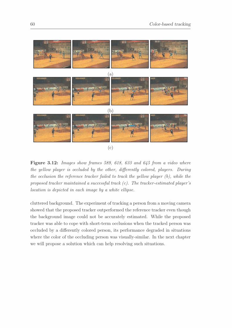
60 Color-based tracking

(a)

(b)

(c)

Figure 3.12: Images show frames 589, 618, 633 and 645 from a video where

the yellow player is occluded by the other, differently colored, players. During

the occlusion the reference tracker failed to track the yellow player (b), while the

proposed tracker maintained a successful track (c). The tracker-estimated player’s

location is depicted in each image by a white ellipse.

cluttered background. The experiment of tracking a person from a moving camera

showed that the proposed tracker outperformed the reference tracker even though

the background image could not be accurately estimated. While the proposed

tracker was able to cope with short-term occlusions when the tracked person was

occluded by a differently colored person, its performance degraded in situations

where the color of the occluding person was visually-similar. In the next chapter

we will propose a solution which can help resolving such situations.

We have gotten stuck half-way in our transition from the

planned and command economy to a normal market

economy. We have created... a hybrid of the two systems.

Boris N. Yeltsin (1931 - 2007)

Chapter 4

Combined visual model

The color-based probabilistic visual model, which was proposed in the previous

section can significantly increase the tracking performance in cases when the

color of the background is similar to the color of the tracked object. However, an

inherent drawback of the color-based (or edge-based for that matter) models is

that tracking may fail whenever the target gets into a close proximity of a visually

similar object. We have observed one such situation in the second experiment of

the previous chapter. There we were tracking a black person through occlusion

by another black person. In that situation, the visual information provided from

the color-based visual model became too ambiguous and after occlusion was over,

the tracker continued to track the wrong person. In applications such as video

surveillance, visual human-computer interface and tracking in sports, the camera

is sometimes positioned such that the scene is viewed from the side only. In

these situations, complete occlusions between visually similar objects are quite

frequent, which is bound to deteriorate the tracking performance of any color-

based tracker.

In this chapter we argue that ambiguities which arise from the visual similarity

between different objects can be resolved to some extent if we account not only

for the target’s color but also its low-level temporal component of the visual

information – the optical flow. We illustrate our argument in Figure 4.1 with an

example of tracking person’s right hand after it has been occluded by the left

hand. Figure 4.1d shows the likelihood function corresponding to the reference

color model of the hand. Observe that the mode of the likelihood function

stretches over both hands. This is causing a persistent ambiguity in the hand’s

position and it is very likely that tracking will fail. Now assume that we calculate

61

62 Combined visual model

the optical flow in the image (Figure 4.1b) and that we know the tracked hand

is moving to the left. If we now visualize the likelihood function reflecting which

flow vectors in (Figure 4.1b) are pointing to the left, we get the local-motion

likelihood function in Figure 4.1e. Note that while one of the modes of the

function corresponds to the tracked hand, the other hand is hidden since it is

not moving to the left. The local-motion likelihood function assigns significant

likelihood also to some other parts of the image which do not correspond to the

tracked hand and is on its own also introducing some ambiguity in the position

of the tracked hand. But if we combine (multiply) the color likelihood with

the local-motion likelihood, we get the combined likelihood function as shown in

Figure 4.1f. Note that now only the mode corresponding to the tracked hand

remains and that the maximum corresponds to the hand’s location (Figure 4.1c)

– we have thus successfully resolved the ambiguity of the hand’s position.

The outline of this chapter is as follows. In Section 4.1 we discuss a method

for estimating the optical flow. Based on this method we define the local-motion

feature in Section 4.2, where we also derive a probabilistic model for the local

motion. The combined, color- and motion-based probabilistic tracker is derived in

Section 4.3 and results of experiments are reported in Section 4.4. We summarize

this chapter in Section 4.5.

4.1 Optical flow

When an object moves through an observed environment, its motion is perceived

by the camera as the changes in intensity of the points in a 3D space. If we assign

a velocity vector to each of those 3D points, then we obtain the so-called motion

field that tells us how each point in the scene is translating with respect to the

camera (see [84], pages 278–285). An image is generated in the camera through

a projection of the light rays of the 3D points onto the CCD sensor. While one

source of changes in the intensity of 3D points is the motion field, the other is the

changing illumination of the scene. These two sources induce temporal patterns

of intensities at the pixels on the CCD sensor. The induced patterns are called

the apparent motion, and an estimate of the apparent motion, which we calculate

from a sequence of images, is called the optical flow.

A widely used hypothesis for calculating the optical flow is that the brightness

of a local structure (e.g., a pixel on a moving object) remains constant over

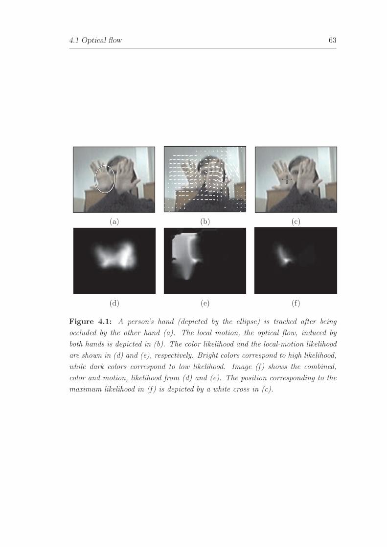
4.1 Optical flow 63

(a) (b) (c)

(d) (e) (f)

Figure 4.1: A person’s hand (depicted by the ellipse) is tracked after being

occluded by the other hand (a). The local motion, the optical flow, induced by

both hands is depicted in (b). The color likelihood and the local-motion likelihood

are shown in (d) and (e), respectively. Bright colors correspond to high likelihood,

while dark colors correspond to low likelihood. Image (f) shows the combined,

color and motion, likelihood from (d) and (e). The position corresponding to the

maximum likelihood in (f) is depicted by a white cross in (c).

64 Combined visual model

consecutive images, while its location may change [16]. This is known as the

data conservation constraint. However, since calculation of the flow vector from a

single pixel is ill-posed, additional constraints are required. Alternatively, one can

assume data conservation within a patch rather than a single pixel and then solve

the optical flow vectors by least squares [103]; this is the basis of the well-known

Lucas-Kanade method. However, since a nonrobust least-squares method is used

in the Lucas-Kanade method, the resulting optical flow is still poorly estimated

in regions of homogeneous intensity, since there the calculation is again ill-posed

and very susceptible to noise. This drawback can be remedied to some extent

by noting that the intensity patterns of the near-by pixels in the image tend to

move similarly. The constraint which assumes similar velocities in the neighboring

pixels is called the spatial coherence constraint. Horn and Schnuck have proposed

a method for calculating the optical flow in [58] which simultaneously applies the

data conservation constraint as well as the spatial coherence constraint. This

method produces a better optical flow than the Lucas-Kanade method but at

a cost of significantly increasing its computation time. In practice, however,

both, the data conservation and spatial coherence constraints are violated in

the presence of multiple motions, and since the underlying calculations are

usually carried out using the least squares, the estimated optical flows may

still contain errors. Some researchers [16] therefore replace the nonrobust least

squares with robust estimators to handle multiple motions, or explicitly model

the discontinuities by generative models [17]. Usually, calculations of flow vectors

with respect to various constrains involve iterative procedures and are thus

computationally very demanding. For that reason, Zach et. al. [173] have recently

proposed efficient implementations that exploit features of specialized graphic

cards to calculate optical flow with spatial and data conservation constraint in

real-time.

To illustrate how constraints influence the calculation of the optical flow we

compare the optical flows estimated using the Lucas-Kanade approach [103] and

Michael J. Black’s [16] multiple motion method in Figure 4.2. Note that while the

Black’s method (Figure 4.2c) produces a much better optical flow than Lucas-

Kanade (Figure 4.2b), the time for calculating the Black’s flow in Figure 4.2

was considerably longer than for calculation of the Lucas-Kanade. On a Celeron

1.5GHz, 500MB RAM laptop, a C++ implementation of the Black’s [18] method

4.1 Optical flow 65

(a) (b) (c)

Figure 4.2: Comparison between the optical flow calculated using the Lucas-

Kanade algorithm and using the M. J. Black’s multiple motion algorithm. The

reference image is shown in (a), while results of the Lucas-Kanade and the Black’s

method are shown in (b) and (c), respectively.

required twelve seconds to calculate the flows of a 288× 360 pixels images, while

Lucas-Kanade [122] required only one second.

Due to a considerable time consumption of the methods that involve multiple

constraints, we will focus in the following on using simple methods like the Lucas-

Kanade algorithm to obtain the information about the local motions in the image.

Thus, rather than calculating the dense optical flow (i.e., optical flow vectors of

each pixel) using a time-consuming method, we will identify which points in

the image contain enough local texture, and calculate flow vectors only at those

points. We will be interested in calculating a sparse flow rather than dense,

which will allow us to use computationally less demanding algorithms for flow

calculation.

4.1.1 Calculating the sparse optical flow

There are two conceptual ways in which the optical flow at a given location in

the image can be defined. One way is to consider from which location in the

previous image the pixel in the current image has been translated. The other is

to consider to which location in the next image the pixel in the current image

will be translated. In our implementations we consider the first definition of the

optical flow. Thus the optical flow at a given point is calculated by estimating

the optical flow vector from the current image back to the previous image, and

reversing its direction. This approach was chosen since it relates the current

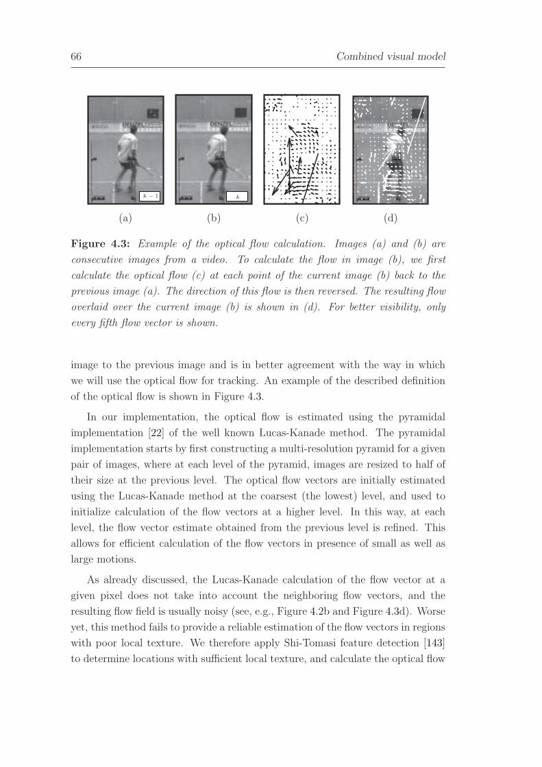
66 Combined visual model

k − 1 k

(a) (b) (c) (d)

Figure 4.3: Example of the optical flow calculation. Images (a) and (b) are

consecutive images from a video. To calculate the flow in image (b), we first

calculate the optical flow (c) at each point of the current image (b) back to the

previous image (a). The direction of this flow is then reversed. The resulting flow

overlaid over the current image (b) is shown in (d). For better visibility, only

every fifth flow vector is shown.

image to the previous image and is in better agreement with the way in which

we will use the optical flow for tracking. An example of the described definition

of the optical flow is shown in Figure 4.3.

In our implementation, the optical flow is estimated using the pyramidal

implementation [22] of the well known Lucas-Kanade method. The pyramidal

implementation starts by first constructing a multi-resolution pyramid for a given

pair of images, where at each level of the pyramid, images are resized to half of

their size at the previous level. The optical flow vectors are initially estimated

using the Lucas-Kanade method at the coarsest (the lowest) level, and used to

initialize calculation of the flow vectors at a higher level. In this way, at each

level, the flow vector estimate obtained from the previous level is refined. This

allows for efficient calculation of the flow vectors in presence of small as well as

large motions.

As already discussed, the Lucas-Kanade calculation of the flow vector at a

given pixel does not take into account the neighboring flow vectors, and the

resulting flow field is usually noisy (see, e.g., Figure 4.2b and Figure 4.3d). Worse

yet, this method fails to provide a reliable estimation of the flow vectors in regions

with poor local texture. We therefore apply Shi-Tomasi feature detection [143]

to determine locations with sufficient local texture, and calculate the optical flow

4.1 Optical flow 67

only at those locations. The Shi-Tomasi feature at location (x, y) is defined by

the smallest eigenvalue of the covariation matrix of gray-scale intensity gradients,

which are calculated in the neighborhood of (x, y). The location (x, y) is accepted

as a valid Shi-Tomasi feature if the smallest eigenvalue exceeds a predefined

threshold ξth. An example of valid Shi-Tomasi features and the corresponding

flow vectors is shown in Figure 4.4. Note that a majority of the flow vectors that

correspond to the valid features in Figure 4.4e appear to be well estimated.

(a) (b)

(c) (d) (e)

Figure 4.4: Two consecutive images from a video of a squash match are shown

in (a) and (b). The optical flow estimated for image (b) using the Lucas-Kanade

method is shown in (c). The valid Shi-Tomasi features are depicted by white color

in image (d). The flow vectors from (c) that correspond to the valid Shi-Tomasi

features in (d) are shown in (e). For clarity, only every third flow vector is shown.

Using the sparse optical flow defined above, we can now derive in the

following the local-motion feature, which will be used later to provide the motion

information for a probabilistic tracker.

68 Combined visual model

4.2 Optical-flow-based local-motion feature

Let vk(x, y) = [r, φ] be the optical flow vector at location (x, y) in the current

image with amplitude r and orientation φ. Note that in the literature the optical

flow vectors are usually written in cartesian coordinates. The reason why we use

the polar notation instead is that in the following we treat the angle of the optical

flow separately from its amplitude. The local-motion feature vE = [rE, φE] of a

region E is then encoded as the weighted average of the flow vectors

vE = f−1v

∑

(x,y)∈E′

vk(x, y)K(x, y), (4.1)

where E ′ ∈ E is a set of detected Shi-Tomasi features within region E, K(x, y) is

the Epanechnikov kernel [140] used to assign higher weights to those flow vectors

that are closer to the center of E, and fv =∑

(x,y)∈E′ K(x, y) is a normalization

term such that fv

∑

(x,y)∈E′ K(x, y) = 1. To avoid the pathological situations

associated with vectors with amplitude zero, the summation (4.1) is carried out

in cartesian coordinates.

4.2.1 Local-motion likelihood

Let vref = [rref , φref ] be a reference vector, which models the target’s local-motion,

and let vE be a local-motion vector calculated within region E. We define the

angular and amplitude similarity Gφ and Gr, respectively, between vref and vE

as

Gφ(vE,vref) =

∠(vE ,vref)π

; rE > δth ∧ rref > δth

1 ; otherwise, (4.2)

Gr(vE,vref) =

|rref−rE |rref+rE

; rE > δth ∨ rref > δth

0 ; otherwise, (4.3)

such that Gφ(·, ·) ∈ [0, 1], Gr(·, ·) ∈ [0, 1], ∠(·, ·) is the angle between two vectors,

| · | is the L1 norm, and δth is a threshold below which the vectors are considered

as having amplitude zero. If region E contains no valid Shi-Tomasi features, the

vector vE is undefined and the similarities are Gφ = 1.0 and Gr = 1.0.

We have observed, in a preliminary study [88], that the probability density

functions (pdf) of (4.2) and (4.3) can be well approximated by exponential

distributions. However, in practice we approximate the current reference motion

4.2 Optical-flow-based local-motion feature 69

using motions observed in previous time-steps. This may impair the quality of

tracking whenever the target suddenly significantly changes its motion. To cope

with such events, we introduce a uniform component to the probability density

function. The joint probability density function of (4.2) and (4.3) with parameters

θ = [λφ, λr, wnoise] is then defined as

p(Gφ, Gr|θ) ∝ (1− wnoise)e−(

Gφλφ

+Grλr

)+ wnoise, (4.4)

where λφ and λr are the parameters of the exponential distributions and

0 < wnoise < 1 is the weight of the uniform component.

4.2.2 Adaptation of the local-motion feature

After each tracking iteration, the current state xk of the target and its current

velocity vk are calculated, e.g., via the MMSE estimate (2.32) from the particle

filter. The new region E containing the target is determined and the local-motion

vector vEk = [φEk, rEk] (4.1) is estimated. If the region E contains at least one

valid Shi-Tomasi feature, then vEk is used to adapt the reference local-motion

model vref = [φref , rref ]. This is achieved by applying an autoregressive scheme

φ+ref = βφkφ

−ref + (1− βφk)φEk,

r+ref = βrkr

−ref + (1− βrk)rEk, (4.5)

where the subscripts (·)− and (·)+, respectively, denote the reference model prior

and after the adaptation. The variables βφk and βrk are the current adaptation

intensities

βφk ∝ p(Gφ(vk,vEk), 0|θ),βrk ∝ p(0, Gr(vk,vEk)|θ), (4.6)

where p(·, ·|θ) is defined in (4.4), and βφk ∈ [0, 1], βrt ∈ [0, 1]. If the region E

does not contain any valid Shi-Tomasi features, then vEk is undefined and the

reference is not adapted.

From (4.6) it follows that the reference local-motion model is adapted to the

local changes in the target’s motion only when the velocity, with which the tracker

predicts the target is moving, is approximately in agreement with the observed

local-motion at the current estimated state. Otherwise the adaptation is low,

since the target is probably being occluded by another object.

70 Combined visual model

4.3 The combined probabilistic visual model

We derive the combined color/local-motion-based visual model by extending the

color-based visual model from Chapter 3 to account for the local-motion. Under

the assumption that the target’s color properties are independent of its motion,

the likelihood function for the particle filter can be written as

p(yk|xk) = p(ykcol|xk)p(ykmot|xk), (4.7)

where p(ykcol|xk) is the color likelihood at state xk, and p(ykmot|xk) presents

the local-motion likelihood at that state. Note that, in the case of the purely

color-based visual model from Chapter 3, Tcol, the likelihood function is equal

to p(ykcol|xk). The combined color/local-motion-based visual model, we denote

it by Tcmb, is then obtained by replacing the likelihood function in Tcol by (4.7)

and setting

p(ykmot|xk) = p(Gφ(vxk,vref), Gr(vxk

,vref)|θ). (4.8)

In the equation above, p(·, ·|θ) is defined in (4.4), vxkis the local-motion (4.1)

sampled at state xk, and vref is the reference local-motion. While, during tracking,

the color histograms are sampled within the elliptical regions of the hypothesized

states x(i)k , we have found that, in practice, it is sufficient to sample the local-

motion feature (4.1) within the rectangular regions superimposed over the ellipses.

The combined color/local-motion-based probabilistic tracker can be derived

from purely color-based tracker (Algorithm 3.1) by using the likelihood function

defined in (4.7, 4.8) and the local-motion adaptation scheme from section 4.2.2.

The combined probabilistic tracker is summarized in Algorithm 4.1.

4.4 Experiments

Several experiments were conducted using examples from surveillance, sports

tracking and hand tracking (Figure 4.5) to compare the proposed combined

tracker Tcmb from Algorithm 4.1 to the purely color-based tracker Tcol proposed

in Algorithm 3.1. Both trackers used 50 particles in the particle filter and a

nearly-constant-velocity dynamic model. All recordings were taken at the frame-

rate of 25 frames per second, except for the recording which was used for hand

tracking; that recording was taken at 30 frames per second.

4.4 Experiments 71

Initialize:

• Initialize the tracker by selecting the target. (e.g. manually)

Tracking:

• For k = 1, 2, 3, . . .

1. Execute an iteration of the color-based particle filter from Algorithm 3.1

using the likelihood function p(yk|xk) defined in (4.7) and the current

reference local-motion vref .

2. Estimate the current MMSE state xk and the current velocity vk using

(2.32).

3. Estimate the new reference vref according to section 4.2.2.

Algorithm 4.1: The combined color/local-motion-based probabilistic tracker.

The Shi-Tomasi feature detection from section 4.2 was performed using 3 ×3 pixels neighborhoods and only features whose smallest eigenvalue exceeded

ξth = 10−3 were accepted. The size of the integration window in the Lucas-Kanade

optical flow calculation was set to 9× 9 pixels. The amplitude threshold used in

(4.2) and (4.3) was set to δth = 10−2 pixels. In the experiment with hand tracking,

a two-level pyramid was used to calculate the optical flow. The pyramids were

not used in the other experiments. The parameters of the local-motion likelihood

function (4.7) were set experimentally to λφ = 0.1, λr = 0.3 and wnoise = 0.01.

Note that, since λr was chosen to be larger than λφ, the amplitude of the local

motion had a smaller impact on the value of the likelihood function in comparison

to the angle. The reasoning behind this is that during an accelerated movement,

typical for hands and people, the amplitude of the optical flow changes more

significantly than its direction. Note that, with the exception of the number of

the pyramid levels, all parameters of the combined visual model were kept fixed

for all experiments. We summarize these parameters in Table 4.1.

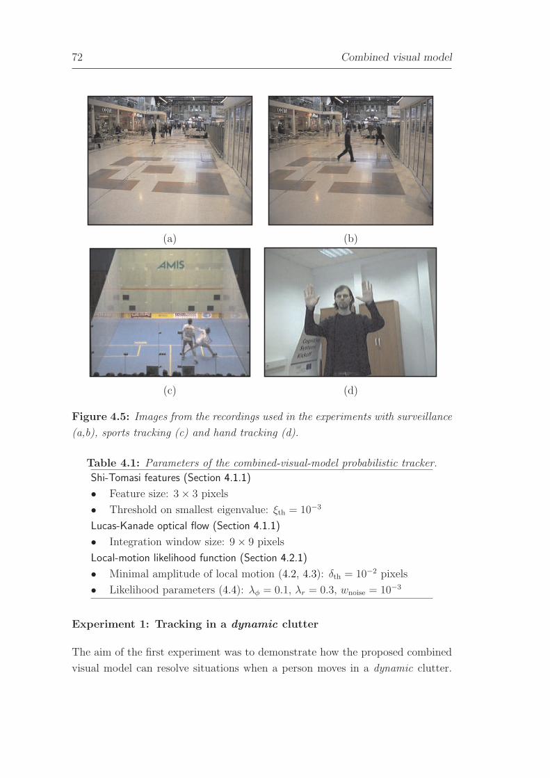
72 Combined visual model

(a) (b)

(c) (d)

Figure 4.5: Images from the recordings used in the experiments with surveillance

(a,b), sports tracking (c) and hand tracking (d).

Table 4.1: Parameters of the combined-visual-model probabilistic tracker.

Shi-Tomasi features (Section 4.1.1)

• Feature size: 3× 3 pixels

• Threshold on smallest eigenvalue: ξth = 10−3

Lucas-Kanade optical flow (Section 4.1.1)

• Integration window size: 9× 9 pixels

Local-motion likelihood function (Section 4.2.1)

• Minimal amplitude of local motion (4.2, 4.3): δth = 10−2 pixels

• Likelihood parameters (4.4): λφ = 0.1, λr = 0.3, wnoise = 10−3

Experiment 1: Tracking in a dynamic clutter

The aim of the first experiment was to demonstrate how the proposed combined

visual model can resolve situations when a person moves in a dynamic clutter.

4.4 Experiments 73

A recording from PETS 2006 database [127] (Figure 4.5a) was chosen, which

contained a black person walking in front of a group of black persons. This group

constituted the so-called dynamic clutter, since this clutter did not come from a

static background. The size of the person in the video was approximately 13×30

pixels. The person was manually selected and tracked with Tcol and Tcmb. The

results of tracking with Tcol are shown in Figure 4.6a. Even though the person

was walking in front of the group, the purely color-based tracker Tcol could not

discern the person from the group when they came into contact due to their visual

similarity, and tracking failed. Note that it is indeed difficult even for a human

observer to discern the tracked person from the others by solely looking at, for

example, 155th frame in Figure 4.6a. On the other hand, the proposed combined

visual model in Tcmb was able to make use of the optical flow information, and

successfully tracked the person throughout the contact (Figure 4.6b).

t=125 t=146 t=155 t=171 t=210

(a)

t=125 t=146 t=155 t=171 t=210

(b)

Figure 4.6: Images from the recording used in the experiment of tracking in a

dynamic clutter. The upper row (a) shows the results for tracking with the purely

color-based tracker Tcol, while the results for the proposed Tcmb are shown in the

bottom row (b). In all images, the current estimated position of the person is

depicted by the white ellipse, while the estimated velocity is depicted by the cyan

line. In the lower-row images (b), the red line depicts the local-motion feature

calculated at the estimated position, while the green line shows the current model

of the local motion.

74 Combined visual model

Experiment 2: Tracking a person through occlusion

In the second experiment we have reconsidered the surveillance scenario

(Figure 4.5b) which was used in the previous chapter to evaluate the performance

of the color-based probabilistic tracker; see Section 3.6. In that scenario, a

person was tracked as he moved from left part of the scene to the right, and

back to the left. While he was walking back to the left, he was occluded for a

short duration by another visually-similar person. Recall that the tracker which

used the color-based visual model proposed in Chapter 3 was able to track that

person even when the person was located on a cluttered background. However,

when that person was occluded by another person, the tracker failed since the

measurements became too ambiguous. The results of tracking with the proposed

combined tracker Tcmb and the purely color-based model in tracker Tcol are shown

in Figure 4.7. Figure 4.7a shows that Tcol fails during the occlusion, which is due

to a significant visual ambiguity of the person’s position. On the other hand,

Tcmb is able to make use of the local-motion, and does not fail (Figure 4.7b).

In particular, the local-motion indicates that the apparent motion of the tracked

target should point to the left. Since the tracked person and the occluding person

are moving in the opposite directions, this helps resolve the visual ambiguity and

allows the tracker to maintain a lock on the correct target.

Experiment 3: Tracking a person through multiple occlusions

To demonstrate how the proposed tracker with a combined model performs in

light of multiple occlusions between visually-similar persons, who rapidly change

their direction of movement, we have considered an example of tracking a player

in a squash match (Figure 4.5c). The tracked player was approximately 25× 45

pixels large and was occluded 14 times by another visually-similar player. The

player was tracked five times, and the average number of times that the tracker

failed was recorded. The purely color-based tracker Tcol failed on average twelve

times, while Tcmb failed on average three times. Figure 4.8a shows five frames

from the recording where, after the occluded player appears (t = 418), the visual

information becomes ambiguous, since both players wear white shirts, and Tcol

fails (t = 425). On the other hand, Tcmb successfully utilizes the local-motion

information to resolve this ambiguity, and tracks the correct player even after the

occlusion (Figure 4.8b).

4.4 Experiments 75

t=651 t=657 t=661 t=664 t=671

(a)

t=651 t=657 t=661 t=664 t=671

(b)

Figure 4.7: Images from the recording used in the experiment of tracking through

an occlusion. The upper row (a) shows the results for tracking with the purely

color-based tracker Tcol, while the results for the proposed Tcmb are shown in the

bottom row (b). In all images, the current estimated position of the person is

depicted by the white ellipse, while the estimated velocity is depicted by the cyan

line. In the lower-row images (b), the red line depicts the local-motion feature

calculated at the estimated position, while the green line shows the current model

of the local motion.

Experiment 4: Tracking person’s palms

In the fourth experiment we have considered a recording of a person waving

his hands (Figure 4.5d) in front of the camera. The hands were approximately

20×20 pixels large, and were tracked independently of each other. They occluded

each other 17 times with majority of occlusions occurring in front of the person’s

face. The reference tracker Tcol failed 26 times, by either following the wrong

hand or the face after the occlusion. The combined tracker Tcmb resolved a

majority of occlusions, and failed only four times by losing the hand and locking

onto the person’s face. A detailed inspection of the results showed that, in the

situations where Tcmb failed, the target’s color model was strongly favoring the

face, while the local-motion feature at the edge of the tracked hand still supported

the target’s reference motion. The reference motion model deteriorated, which

caused the tracker to drift from the hand to the face. Figure 4.9 shows an example

where Tcol lost the hand after it was occluded by another hand (Figure 4.9a),

while Tcmb resolved the occlusion (Figure 4.9b).

76 Combined visual model

t=407 t=411 t=414 t=418 t=425

(a)

t=407 t=411 t=414 t=418 t=425

(b)

Figure 4.8: Images from the recording used in the experiment of tracking a

person through multiple occlusions. The upper row (a) shows the results for

tracking with the purely color-based tracker Tcol, while the results for the proposed

Tcmb are shown in the bottom row (b). In all images, the current estimated

position of the person is depicted by the white ellipse, while the estimated velocity

is depicted by the cyan line. In the lower-row images (b), the red line depicts

the local-motion feature calculated at the estimated position, while the green line

shows the current model of the local motion.

4.5 Conclusion

In this chapter we have proposed a combined visual model for probabilistic

tracking which is composed of two visual models of the tracked object. The

first model is the color-based model which we have proposed in Chapter 3.

Since this model alone cannot resolve situations when the tracked object gets

into a close proximity of another, visually similar object, we have proposed a

novel visual model, which we call the local motion. The local-motion model was

presented in Section 4.2, where we have shown how it can be calculated from the

optical flow (Section 4.1.1) which is estimated using the Lucas-Kanade algorithm.

While the Lucas-Kanade algorithm is relatively fast, it gives poor estimates of

the optical flow in regions which lack texture. For that reason, we use the Shi-

Tomasi features to detect regions with enough texture and estimate the optical

flow only at those regions. Thus the local-motion is defined using only a sparse

optical flow. To account for the errors in the optical flow estimation and rapid

changes in the target’s motion, we have derived a probabilistic model of the

4.5 Conclusion 77

t=22 t=29 t=32 t=35 t=45

(a)

t=22 t=29 t=32 t=35 t=45

(b)

Figure 4.9: Images from the recording used in the experiment of tracking person’s

hands. The upper row (a) shows the results for tracking with the purely color-

based tracker Tcol, while the results for the proposed Tcmb are shown in the bottom

row (b). In all images, the current estimated position of the person is depicted by

the white ellipse, while the estimated velocity is depicted by the cyan line. In the

lower-row images (b), the red line depicts the local-motion feature calculated at

the estimated position, while the green line shows the current model of the local

motion.

local-motion in Section 4.2.1. Since the local-motion model significantly changes

during the target’s movement, an adaptation scheme for the local-motion model

was devised in Section 4.2.2. In Section 4.3 we have shown how the proposed

local-motion model can be probabilistically combined with the color-based model

into the combined probabilistic visual model. We have also proposed a particle-

filter-based tracker which uses the combined model.

Several experiments have been carried out to demonstrate improvement of

tracking performance when using the combined model instead of a purely color-

based model. Experiments included tracking persons in a dynamic clutter,

tracking through occlusions and an example of tracking a persons’s hands through

multiple occlusions. The experiments have clearly shown the superiority of the

combined model over the purely color-based model by significantly reducing the

number of failures during tracking.

Since the proposed combined tracking scheme can help resolve ambiguities

associated with multiple visually similar targets, it can be used as an extension

78 Combined visual model

to existing multiple-target tracking schemes, such as [141], to increase their

robustness. Note also that the local-motion-based feature (Section 4.2) is general

enough to be used not only within the framework of particle filters, but also with

non-stochastic methods, e.g., the recently proposed AdaBoost tracker [54], to

resolve the ambiguities caused by the visual similarity between different objects.

And yet it moves.

Galileo Galilei (1564-1642)

Chapter 5

A two-stage dynamic model

In the previous two chapters we have explored two different visual models of the

target to improve tracking in light of poor visual information. In this chapter, we

will focus on another important part of the probabilistic tracker – the dynamic

model by which we describe the dynamics of the tracked target. If the dynamics

are well modelled, then the tracker’s performance can be improved in several ways.

One improvement may be more accurate estimates of the target’s position and

prediction, while the other is a smaller failure rate. Note that since the particle

filters are Monte Carlo methods, the accuracy of target’s estimates depends on

the number of particles used in the filter. Larger numbers of particles allow denser

coverage of the target’s state space and usually result in a more accurate tracking.

However, using more particles means more evaluations of the likelihood model.

Depending on the complexity of the target’s visual model, these evaluations can

be time-consuming, and can significantly slow down the tracking. By choosing an

appropriate dynamic model, the particles can be used more efficiently. This can

be achieved by directing them into the regions of the state space, which are more

likely to contain the current state of the target. Smaller number of particles may

therefore be used to achieve equal or even better accuracy than a poorer dynamic

model would have achieved with a larger number of particles. In this sense, at a

fixed accuracy, a proper dynamic model can effectively reduce the computation

time required for a single tracking iteration and making the tracking feasible for

real-time applications.

When tracking persons, one of the following two models is used in practice:

the random-walk (RW) model or the nearly-constant-velocity (NCV) model. The

simplest of the two models, the RW model, assumes that velocity can be modelled

79

80 A two-stage dynamic model

by a white noise process and is appropriate when the target performs radical

accelerations in different directions; for example, when a person suddenly changes

direction of its motion or suddenly stops. On the other hand, in cases when the

target moves in a certain direction, the RW model usually performs poorly and

the motion is much better described by the NCV model. Unlike the RW model,

the NCV model assumes that the acceleration can be modelled by a white noise

process. While it is true that at times human motion can be explained best by

either the RW or the NCV model, the motion is often somewhere in between

the two models. In this chapter we propose a two-stage dynamic model which

is able to better model the dynamics of the human motion. We call the model

a ”two-stage” dynamic model due to its particular structure, which is composed

of two different models: a liberal and a conservative model. The liberal model

allows larger perturbations in the target’s dynamics and is able to account for

motions in between RW and NCV. On the other hand, the conservative model

assumes smaller perturbations and is used to further adapt the liberal model

to the current dynamics of the tracked object. We also propose a two-stage

probabilistic tracker based on the particle filter and apply it to tracking entire

persons as well as person’s hands.

The outline of this chapter is as follows. In Section 5.1 we develop the

liberal dynamic model and analyze how the parameters of the model influence

the model’s structure. The conservative model is proposed in Section 5.2 and

in Section 5.3 we propose the two-stage dynamic model and the corresponding

probabilistic tracker. In Section 5.4 results of the experiments are reported, and

we summarize the chapter in Section 5.5.

5.1 The liberal dynamic model

As noted, the RW model assumes that the target’s velocity is a white-noise

sequence and is thus temporally completely noncorrelated. On the other hand,

the NCV model assumes that velocity is temporally strongly correlated, since the

changes in velocity arise only due to the white noise of the acceleration. Thus

the conceptual difference between RW and NCV models is that they assume two

extremal views on the temporal correlation of the velocity. With this rationale we

can arrive at a more general model by simply treating the velocity as a correlated

noise, but without deciding on the extent to which it is correlated. A convenient

5.1 The liberal dynamic model 81

way to model the correlated noise is to use a Gauss-Markov process (GMP). The

GMP has been previously used with some success (see, e.g., [146, 147, 176]) in

modelling the acceleration of an airplane in flight, which allowed an improved

tracking during air maneuvers. In this section we show that by modelling

the velocity with a Gauss-Markov process, we arrive at a model of which RW

and NCV are only special cases and which is able to account for more general

dynamics; we will call this model the liberal model. We also provide an analysis

of the parameters of the liberal model.

We start by noting that changes in the position x(t) arise due to a non-zero

velocity v(t) of the target, i.e., x(t) = v(t). The velocity v(t) is then modelled as

a non-zero-mean correlated noise

v(t) = v(t) + v(t), (5.1)

where v(t) denotes a zero-mean correlated noise and v(t) is the current mean of

the noise – the input velocity. We model the correlated noise v(t) as a Gauss-

Markov process with an autocorrelation function Rv(τ) = σe−β|τ |, where σ2 is the

variance of the process noise, and β is the correlation time constant. To derive

the dynamic model of the process (5.1) in a form which we can use for tracking,

we have to first find a stochastic differential equation (s.d.e.) of the process (5.1),

governed by a white-noise process, and then find its discretized counterpart.

To derive the s.d.e. of the the process v(t) in (5.1), with the correlation

function Rv(τ), we have to find a shaping filter (see, e.g., [26], page 137), with a

system transfer function G(s)1, which transforms a unity-white noise u(t) into

v(t) (see Figure 5.1). In principle, the transfer function G(s) can be easily

found from the spectral densities of the input u(t) and the output v(t) of the

system shown in Figure 5.1. Although the derivation of the shaping filter can

be usually found in textbooks on theory of estimation and control, we provide

a summarized derivation here for completeness. We start by noting that, for a

stationary process, the Wiener-Khinchine relation (see, e.g., [26], page 86) tells

us that the spectral density Sv(s) of the process v(t) is given by the Fourier

transform F [·] of the process autocorrelation function Rv(τ); therefore we have

Sv(s) = F [Rv(τ)] =2σ2β

β2 − s2. (5.2)

1We use s to denote the complex frequency jw, where w has the usual meaning of the

frequency in hertz.

82 A two-stage dynamic model

u(t) G(s) v(t)

Figure 5.1: A shaping filter G(s) that takes a unity white-noise signal u(t) and

transforms (shapes) it into v(t).

It can also be shown (see, e.g., [26], page 130) that the spectral density Su(s) of

the input u(t) and the spectral density Sv(s) of the output v(t) of the system in

Figure 5.1 are related as

Sv(s) = G(s)G(−s)Su(s). (5.3)

Since the spectral density of the unity-white noise is unity, i.e., Su(s) = 1, we

have from (5.2) and (5.3)

Sv(s) = G(s)G(−s)1 = F [Rv(τ)], (5.4)

which gives the system transfer function, i.e. the shaping filter,

G(s) =

√

2σ2β

s + β. (5.5)

A stochastic differential equation that corresponds to the shaping filter (5.5) is

exactly the s.d.e. which we seek and is given as

˙v(t) = −βv(t) +√

qcu(t), (5.6)

where qc = 2βσ2 is the spectral density of the equivalent white-noise process

acting on ˙v(t) and where, as before, u(t) denotes a unit-variance white-noise

process.

The continuous-time s.d.e. of (5.1) can now be derived by expressing v(t) in

(5.1) and plugging it into (5.6),

˙v(t) = −βv(t) + βv(t) +√

qcu(t). (5.7)

In order to arrive at a discretized form of the above model, we first note from

(5.1) that ˙v(t) = ∂∂t

(v(t)− v(t)) and assume that the input velocity v(t) remains

constant over a sampling interval. Thus we obtain

v(t) = −βv(t) + βv(t) +√

qcu(t). (5.8)

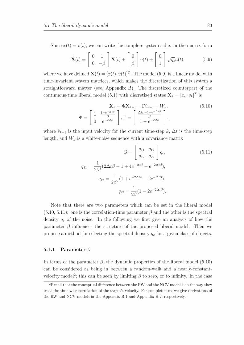
5.1 The liberal dynamic model 83

Since x(t) = v(t), we can write the complete system s.d.e. in the matrix form

X(t) =

[

0 1

0 −β

]

X(t) +

[

0

β

]

v(t) +

[

0

1

]

√qcu(t), (5.9)

where we have defined X(t) = [x(t), v(t)]T. The model (5.9) is a linear model with

time-invariant system matrices, which makes the discretization of this system a

straightforward matter (see, Appendix B). The discretized counterpart of the

continuous-time liberal model (5.1) with discretized states Xk = [xk, vk]T is

Xk = ΦXk−1 + Γvk−1 + Wk, (5.10)

Φ =

[

1 1−e−∆tβ

β

0 e−∆tβ

]

, Γ =

[

∆tβ−1+e−∆tβ

β

1− e−∆tβ

]

,

where vk−1 is the input velocity for the current time-step k, ∆t is the time-step

length, and Wk is a white-noise sequence with a covariance matrix

Q =

[

q11 q12

q12 q22

]

qc, (5.11)

q11 =1

2β3(2∆tβ − 1 + 4e−∆tβ − e−2∆tβ),

q12 =1

2β2(1 + e−2∆tβ − 2e−∆tβ),

q22 =1

2β(1− 2e−2∆tβ).

Note that there are two parameters which can be set in the liberal model

(5.10, 5.11): one is the correlation-time parameter β and the other is the spectral

density qc of the noise. In the following we first give an analysis of how the

parameter β influences the structure of the proposed liberal model. Then we

propose a method for selecting the spectral density qc for a given class of objects.

5.1.1 Parameter β

In terms of the parameter β, the dynamic properties of the liberal model (5.10)

can be considered as being in between a random-walk and a nearly-constant-

velocity model2; this can be seen by limiting β to zero, or to infinity. In the case

2Recall that the conceptual difference between the RW and the NCV model is in the way they

treat the time-wise correlation of the target’s velocity. For completeness, we give derivations of

the RW and NCV models in the Appendix B.1 and Appendix B.2, respectively.

84 A two-stage dynamic model

of β → 0, the model takes the form of a pure NCV model with a state transition

matrix Φβ→0 and the input matrix Γβ→0

Φβ→0 =

[

1 T

0 1

]

, Γβ→0 =

[

0

0

]

. (5.12)

On the other hand, at β → ∞, the model takes the form of a RW model with

the state transition matrix Φβ→∞ and the input matrix Γβ→∞

Φβ→∞ =

[

1 0

0 0

]

, Γβ→∞ =

[

1

1

]

. (5.13)

Note that the values of Γβ→∞ are nonzero, thus the input velocity has to be set

to zero, vk−1 = 0, to obtain the pure random-walk model. For comparison of the

system and input matrices (5.12, 5.13) with those of a NCV and RW model, see

Appendix B.1 and Appendix B.2.

We have seen thus far that the liberal dynamic model takes the structure of

RW and NCV models at the limiting values of β. But what happens when β is

set to somewhere in between zero and infinity? To get a better understanding of

that, it is beneficial to rewrite the model in the following way. Let xk = [xk, vk]T

denote the state at the time-step k with position xk and velocity vk, and, similarly,

let xk−1 = [xk−1, vk−1]T denote the state at the previous time-step k− 1. We also

rewrite the elements of the system transition matrix Φ and the input matrix Γ

(5.10) in the following abbreviated form

Φ =

[

1 φ1,2

0 φ2,2

]

, Γ =

[

γ1

γ2

]

.

Note from (5.10) that Φ and Γ depend on the size of the time-step ∆t, which

is the time between one and the next measurement. Without loss of generality

we can set the time-step to unity ∆t = 1. For completeness, let us also define the

values of the noise terms, at time-step k, acting on the position and velocity by

Wk = [wxk, wvk]T . Now we can rewrite the liberal model (5.10) in terms of the

state’s components as

xk = xk−1 + φ1,2vk−1 + γ1vk−1 + wxk (5.14)

vk = φ2,2vk−1 + γ2vk−1 + wvk.

Since we have set ∆t = 1, we have from (5.10) and (5.14)

φ1,2 + γ1 ≡ 1 and φ2,2 + γ2 ≡ 1.

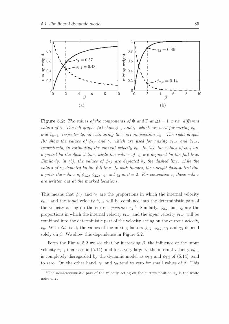
5.1 The liberal dynamic model 85

0 2 4 6 8 100

0.2

0.4

0.6

0.8

1m

ixin

gw

eigh

t

φ1,2 = 0.43

γ1 = 0.57

β0 2 4 6 8 10

0

0.2

0.4

0.6

0.8

1

mix

ing

wei

ght

φ2,2 = 0.14

γ2 = 0.86

β

(a) (b)

Figure 5.2: The values of the components of Φ and Γ at ∆t = 1 w.r.t. different

values of β. The left graphs (a) show φ1,2 and γ1 which are used for mixing vk−1

and vk−1, respectively, in estimating the current position xk. The right graphs

(b) show the values of φ2,2 and γ2 which are used for mixing vk−1 and vk−1,

respectively, in estimating the current velocity vk. In (a), the values of φ1,2 are

depicted by the dashed line, while the values of γ1 are depicted by the full line.

Similarly, in (b), the values of φ2,2 are depicted by the dashed line, while the

values of γ2 depicted by the full line. In both images, the upright dash-dotted line

depicts the values of φ1,2, φ2,2, γ1 and γ2 at β = 2. For convenience, these values

are written out at the marked locations.

This means that φ1,2 and γ1 are the proportions in which the internal velocity

vk−1 and the input velocity vk−1 will be combined into the deterministic part of

the velocity acting on the current position xk.3 Similarly, φ2,2 and γ2 are the

proportions in which the internal velocity vk−1 and the input velocity vk−1 will be

combined into the deterministic part of the velocity acting on the current velocity

vk. With ∆t fixed, the values of the mixing factors φ1,2, φ2,2, γ1 and γ2 depend

solely on β. We show this dependence in Figure 5.2.

Form the Figure 5.2 we see that by increasing β, the influence of the input

velocity vk−1 increases in (5.14), and for a very large β, the internal velocity vk−1

is completely disregarded by the dynamic model as φ1,2 and φ2,2 of (5.14) tend

to zero. On the other hand, γ1 and γ2 tend to zero for small values of β. This

3The nondeterministic part of the velocity acting on the current position xk is the white

noise wxk.

86 A two-stage dynamic model

means that we can consider β as a parameter that specifies an a-priori confidence

of the input vk−1 and internal velocity vk−1. If, for example, we know that vk−1

is very accurate, then β should be set to a very large value. Otherwise, smaller

β should be used.

The two-stage dynamic model which is presented in this chapter usually yields

reasonable estimates of the input velocity vk−1 for a large class of targets. In

practice we have observed that it is thus beneficial to let the input velocity vk−1

have a dominant effect over vk−1 in estimating the current velocity vk. However,

if we want the liberal model to be able to account for a greater agility of the

target, it is also beneficial to let the internal velocity vk−1 to have a greater effect

on predicting the current position xk. We have found that these requirements

are sufficiently well met at β ≈ 2 which is the value we use in all subsequent

experiments. The values of φ1,2 and γ1 at β = 2 are shown in Figure 5.2a, while

the values of φ2,2 and γ2 at β = 2 are shown in Figure 5.2b.

5.1.2 Selecting the spectral density

Another important parameter of the liberal model (5.10) is the spectral density qc

of the process noise (5.11). Note that in many cases it is possible to obtain some

general characteristics of the dynamics of the class of objects which we want to

track. Specifically, the expected squared distance σ2m that objects of certain class

travel between two time-steps is often available. Assuming that we have some

estimate of σ2m, and that the time-step size ∆t and the parameter β are known,

we now derive a rule-of-thumb rule for selecting the spectral density qc.

To derive the rule-of-thumb, let us consider the following example. Assume

that at time-step k − 1 a target is located at the origin of the coordinate

system, i.e., xk−1 = 0, and begins moving with a velocity vk−1 ∼ q22qc, i.e.,

Xk−1 = [0, vk−1]T. Assuming that the input velocity vk−1 in (5.10) is zero, the

target’s state after a single time-step is

Xk = ΦXk−1 + Wk. (5.15)

The covariance of the position at time-step k is

P = 〈XkXTk 〉

= 〈ΦXk−1XTk−1Φ

T 〉+ 〈ΦXk−1WTk 〉+ 〈WkX

Tk−1Φ

T 〉+ 〈WkWTk 〉, (5.16)

5.2 The conservative dynamic model 87

where 〈·〉 denotes the expectation operator. Since the state Xk−1 is not correlated

with the noise Wk and since Q∆=〈WkW

Tk 〉, the equation (5.16) simplifies into

P =

[

p11 p12

p21 p22

]

= Φ〈Xk−1XTk−1〉ΦT + Q. (5.17)

Since p11 in (5.17) is just the expected squared change of target’s position in

consecutive time steps, i.e. p11 = σ2m, we have

σ2m = p11

= (1− e−∆tβ

β)2〈vk−1vk−1〉+ q11qc. (5.18)

Since we have defined earlier vk−1 ∼ q22qc, we know that 〈vk−1vk−1〉 = q22qc, and

(5.18) is rewritten into

σ2m = ((

1− e−∆tβ

β)2q22 + q11)qc. (5.19)

Inverting (5.19) finally gives the rule-of-thumb rule for selecting the spectral

density

qc = σ2m((

1− e−∆tβ

β)2q22 + q11)

−1. (5.20)

5.2 The conservative dynamic model

In the previous section we have presented a liberal dynamic model (5.10) which

we have derived from a continuous-time non-zero-mean Gauss-Markov process.

While a detailed discussion of how different parameters of the Gauss-Markov

process (GMP) influence the structure of the liberal model was provided, we

have not said anything about estimating the mean value of the GMP, which we

have named the input velocity vk−1 (5.10). In this section we propose another

dynamic model, a conservative dynamic model, which will serve for estimating

vk−1 during tracking, and thus further adapt the liberal model to the current

dynamics of the tracked object. The conservative model assumes that the target’s

velocity does not change abruptly and approximates the local dynamics by fitting

a linear model to the past filtered states. This model is then used to regularize

the estimated target states from the particle filter, as well as for estimating the

input velocity vk−1 of the liberal model.

88 A two-stage dynamic model

Let ok−K:k−1 = oik−1i=k−K denote a sequence of the K past regularized states

oi of the tracked target and let πk−K:k−1 = πik−1i=k−K denote the set of their

weights. These weights indicate how well the corresponding states have been

estimated. The conservative model aims to locally approximate the sequence

ok−K:k−1 by a linear model

o(ti) = vk−1ti + ak−1, (5.21)

where ti is the time at i-th time step. Since all states have not been estimated

equally well, and since the recent states bare more information about the current

velocity of the target, the parameters vk−1 and ak−1 of the linear model (5.21)

are estimated such that they minimize the following weighted sum of squared

differences

Ck−1 =k−1∑

i=k−K

G(i)k−1d

Ti di , di = oi − vk−1ti − ak−1, (5.22)

where the weights G(i)(·) are defined as

G(i)j = π(i)e

− 12

(i−j)2

σ2o . (5.23)

While the first term in (5.23) reflects the likelihood of the state oi, the second

term is a Gaussian which assigns higher a-priori weights to the more recent states.

In practice this means that we only consider K = 3σo past states in (5.22), since

the a-priori weights of all the older states are negligible. Note that the Gaussian

form was used for the last term exclusively to attenuate the importance of the

older states. In general, however, other forms that exhibit similar behavior (e.g.,

an exponential function) could have been used.

From (5.22) we can now find vk−1 and ak−1 simply by setting the

corresponding partial derivatives to zero

∂Ck−1

∂vk−1

∆=0 ,

∂Ck−1

∂ak−1

∆=0, (5.24)

which gives

vk−1 =

k−1∑

i=k−K

tiG(i)k−1oi + Ak−1(

k−1∑

i=k−K

G(i)k−1oi)(

k−1∑

i=k−K

tiG(i)k−1)

k−1∑

i=k−K

t2i G(i)k−1 − Ak−1(

k−1∑

i=k−K

tiG(i)k−1)

2

, (5.25)

ak−1 = Ak−1(k−1∑

i=k−K

G(i)k−1oi − vk−1

k−1∑

i=k−K

tiG(i)k−1), (5.26)

5.3 A two-stage dynamic model 89

where we have defined

Ak−1 = (k−1∑

i=k−K

G(i)k−1)

−1. (5.27)

Once the parameters of the conservative model (5.21) are obtained, the input

velocity of the liberal model (5.10) is approximated by the locally-regularized

velocity vk−1 (5.25), and the regularized state ok of the target is calculated as

follows. The estimate of the target’s state xk is calculated from the liberal model

and fused with the prediction o(tk) (5.21) of the conservative model according to

their visual likelihoods wxk= p(yk|xk) and wo(tk) = p(yk|o(tk)), respectively4, as

ok =o(tk) · wo(tk) + xk · wxk

wo(tk) + wxk

. (5.28)

The corresponding weight πk of the new regularized state ok is evaluated using the

visual likelihood function, πk = p(yk|ok), and the parameters of the conservative

model (5.21) are recalculated using (5.25). The regularized prediction from the

two-stage dynamic model can then be calculated using the following relation

ok+1 = ok + ∆tvk. (5.29)

5.3 A two-stage dynamic model

In Section 5.1 we have presented a liberal model (5.10) which was derived

from a continuous-time non-zero-mean Gauss-Markov process and is capable

of accounting for various types of dynamics, ranging from a random walk to

the nearly-constant-velocity behavior. In Section 5.2 another model, called the

conservative dynamic model, was presented. The conservative model applies

stronger constraints on the target’s velocity and is used for estimating the mean

value (input velocity) of the Gauss-Markov process in the liberal model. In this

section we propose a two-stage dynamic model, which probabilistically combines

the conservative and the liberal model and is applied to probabilistic tracking

using a particle filter. We call the resulting tracker a two-stage probabilistic

tracker and the structure of this tracker is shown in Figure 5.3. Since the liberal

dynamic model allows greater perturbations in the target’s dynamics, we use it

4The visual likelihoods p(yk|xk) and p(yk|o(tk)) refer to the likelihood function used in the

particle filter, like the color-based likelihood function presented in Chapter 3, the combined

likelihood function presented in Chapter 4 or any other appropriate visual likelihood function.

90 A two-stage dynamic model

Particle filter

Conservative dyn. model

Liberal dyn. model

ok

xk

vk−1

Figure 5.3: The structure of the two-stage probabilistic tracker. The liberal

model is embedded into a particle filter and used to estimate the target’s current

state xk. The conservative model, on the other hand, is used to estimate the mean

value (the input velocity) vk−1 of the Gauss-Markov process in the liberal model as

well as to regularize the output of the particle filter xk into an improved estimate

ok of the target’s state.

within the particle filter to efficiently explore the target’s state space. On the

other hand, the conservative model assumes smaller perturbations in dynamics

and is used to estimate the input velocity of the liberal model, as well as for

regularizing the output of the particle filter in light of the visual observations.

The output of the tracker is thus an improved, regularized, estimate of the target’s

state.

An iteration of the proposed two-stage probabilistic tracker proceeds as

follows. First, an input velocity vk−1 for the liberal model (5.10) is estimated

from the conservative model by the locally-regularized velocity vk−1 (5.25). Then

a tracking iteration of a particle-filter-based tracker which uses the liberal model

is carried out. The posterior of the target’s state becomes available from the

particle filter and is used to estimate the new MMSE state xk of the target (2.32).

A prediction o(tk) of the regularized state is calculated from the conservative

model (5.21) and a weight wo(tk) = p(yk|o(tk)) is assigned to the prediction

according to the visual likelihood function p(yk|o(tk))5. Similarly, a weight

wxk= p(yk|xk) is assigned to the MMSE estimate xk which is then fused with

o(tk) according to (5.28) into the new regularized state ok, and the regularized

velocity vk is recalculated using (5.25). The entire tracking procedure of the

two-stage probabilistic tracker is summarized in Algorithm 5.1.

5In our implementations we use the same color-based likelihood function as in the particle

filter.

5.3 A two-stage dynamic model 91

Initialize:

• Initialize the tracker by selecting the target (e.g., manually).

Tracking:

• For k = 1, 2, 3, . . .

1. Approximate the current input velocity vk−1 of the liberal model by the

locally-regularized velocity vk−1 from the conservative model (5.25).

2. Carry out a tracking iteration of the particle-filter-based tracker using the

liberal model (5.10).

3. Calculate the MMSE estimate xk (2.32) from the posterior obtained from

the particle filter.

4. Calculate the conservative prediction o(tk) from the conservative model

(5.21).

5. Fuse the conservative prediction o(tk) with the MMSE estimate xk

according to their respective visual likelihoods into a new regularized state

ok using (5.28).

6. Evaluate the visual likelihood of the regularized state ok and update the

parameters of the conservative model.

Algorithm 5.1: The two-stage probabilistic tracker.

Since the two-stage dynamic model is composed of the liberal and the

conservative model, there are a few parameters that have to be set. Two

parameters have to be set for the liberal model (5.10): the parameter β and

the spectral density qc of the process noise. A detailed discussion of how

the parameter β influences the structure of the liberal model was provided in

Section 5.1.1. There we have concluded, that the required dynamic properties of

the liberal model are met at β = 2. The remaining parameter of the liberal model,

the spectral density qc, has to be specified for the problem at hand and we have

proposed a principled way to selecting qc in Section 5.1.2. The conservative model

requires setting a single parameter σo, which effectively determines the number

of the recent regularized states which are considered in the linearization. We set

92 A two-stage dynamic model

this parameter using the following rationale. We can assume that the objects

which are considered in our applications do not usually change their velocity

drastically within a half of the second. Since most of our recordings used in the

experiments are recorded at 25 frames per second, this means that we consider

only K = 1225 ≈ 13 recent regularized states. We have noted in Section 5.2

that K = 3σo, which means that σo = 4.3. For convenience, we summarize the

parameters in Table 5.1.

Table 5.1: Parameters of the two-stage dynamic model.

The liberal dynamic model (Section 5.1)

• Parameter β = 2.

• Spectral density qc is selected by the rule-of-thumb rule (Section 5.1.2)

The conservative dynamic model (Section 5.2)

• Parameter σo = 4.3.

5.4 Experimental study

We carried out two sets of experiments to evaluate the performance of the two-

stage dynamic model from Section 5.3. In the first experiment (section 5.4.1) we

have tracked persons moving on a predefined path on the ground. This experiment

was designed for quantitative and qualitative comparison between the proposed

two-stage dynamic model and two widely used dynamic models. To demonstrate

the generality of the proposed dynamic model, we have also applied it to tracking

person’s hands in the second experiment (section 5.4.2).

5.4.1 Experiment 1: Tracking entire persons

Seven players of handball were instructed to run on a predefined path drawn on

the court (Figure 5.4). The path was designed such that the observed motion

involved accelerations, decelerations and rapid changes in the direction of motion.

The scene was recorded with a camera mounted on the ceiling of the sport’s hall,

such that the size of each player was approximately 10×10 pixels. The video was

recorded at the frame rate of 25 frames per second. Each player was manually

tracked thirty times through each frame and the average of the thirty trajectories

5.4 Experimental study 93

obtained for each player was taken as the ground truth. In this way approximately

273 ground-truth positions pk = (xk, yk) per player were obtained.

1 2 3 4 5 6 7

Figure 5.4: Seven players and the path used in the first experiment.

All seven players from Figure 5.4 were then tracked with three trackers: Two

reference trackers and the proposed tracker. The only difference between these

trackers was in the dynamic models they used for modelling the dynamics of

the player’s position. The proposed tracker, we denote it by TTS, was the two-

stage probabilistic tracker from Algorithm 5.1, which modelled the dynamics of

the player’s position with the two-stage dynamic model. The reference trackers

were essentially the color-based particle filters from Chapter 3, which employed

two widely-used dynamic models on the player’s position. The first reference

tracker, TRW, used the random-walk model, while the second reference tracker

used the nearly-constant-velocity model; we denote this tracker by TNCV. All

three trackers used random-walk models to model the dynamics of the player’s

size.

The parameters of the RW and NCV dynamic models in TNCV and TRW were

learned from the ground truth. In particular, the only parameter of the RW and

NCV model that has to be specified is the spectral density of the process noise

(see, e.g., equations B.10 and B.13 in Appendix B). The spectral densities were

estimated using a linear-dynamic-system learning method (see, e.g., [15] pages

94 A two-stage dynamic model

635-644)6 from 7× 30 = 210 ground truth trajectories. The method yielded the

spectral density qRW = 4.6 for the RW model and the spectral density qNCV = 0.4

for the NCV model. We have observed in experiments that the estimated spectral

density for RW was too small and, in practice, tracking was failing frequently for

some of the players. For that reason, the spectral density in the RW model was

increased to qRW = 6 in the experiments.

The spectral density qc of the liberal model (5.10) in TTS was determined using

the rule-of-thumb rule, which we have proposed in Section 5.1.2. Recall that the

rule requires us to provide an estimate of the squared distance σ2m that the objects

under consideration are expected to travel between two time steps. Since we track

sports players in our experiment, we can find σ2m as follows. Based on the findings

of Bon et al. [21], who refer to Kotzamanidis [85], Erdmann [46] and Bangsbo [8]

regarding the dynamics of handball/soccer players, we can estimate the highest

velocity of a player as vmax = 8.0m/s. At a frame rate of 25frames/s we can say

that vmax = 0.32m/frame. During tracking, the player is usually determined by

an ellipse that is approximately the size of his/hers shoulders. We estimate this

size to be Ht ≈ 0.4m. Assuming a Gaussian form of the velocity distribution,

the highest velocity can be approximated with three standard deviations of the

Gaussian. This gives vmax = 3σxy/frame and the parameter σm = Ht0.323·0.4

.= Ht

14.

Using the rule-of-thumb rule (5.20) the spectral density of the liberal model is

thus estimated as

qc = (Ht14)2(q11 + q22(

1−e−β

β)2)−1, (5.30)

where q11 and q22 are defined in (5.11).

Quantitative evaluation

Using the parameters given above, all seven players from Figure 5.4 were tracked

thirty times with the trackers TRW, TNCV and TTS. Thus K = 30 trajectories

per player were recorded for each tracker. Note that TRW and TNCV have failed

during tracking on a few occasions by losing the player. In those situations,

6Conceptually, the linear-dynamic-system learning method is an expectation maximization

(EM) algorithm that iterates between two steps. In the first step (the expectation), the

trajectories are filtered using a forward-backward Kalman filtering with the estimated system

parameters to infer the hidden, true, trajectory. In the next step (the maximization), the filtered

trajectories and the corresponding uncertainties are used to re-estimate the system parameters.

5.4 Experimental study 95

tracking was repeated and only the trajectories where tracking did not fail were

considered for evaluation. In all experiments TTS never failed.

A standard one-sided hypothesis testing [10] was applied to determine whether

the accuracy of estimation by TTS was greater than the accuracy of the reference

trackers TRW and TNCV. In the following, when not referring to a specific

tracker, we will abbreviate the reference trackers by TREF. The performance of

the trackers in the r-th repetition was defined in terms of the root-mean-square

(RMS) error as

C(r) ∆=

1

7

7∑

i=1

(1

K

K∑

k=1

‖(i)pk − (i)p(r)k ‖2)

12 . (5.31)

In (5.31) (i)pk denotes the ground-truth position at time-step k for the i-th player,(i)p

(r)k is the corresponding estimated position and ‖ · ‖ is the l2 norm. At each

repetition, a sample-performance-difference

∆(r) = C(r)REF − C

(r)TS (5.32)

was calculated. The term C(r)TS was the cost value (5.31) of TTS, while C

(r)REF

presented the cost value of the reference tracker TREF .

In our case the null hypothesis H0 was that TTS is not superior to TREF. For

each tracker we calculated the sample-performance-difference mean

∆ =1

R

∑R

r=1∆(r) (5.33)

and its standard error

σ∆ =

√

√

√

√

1

R2

R∑

r=1

(∆(r) − ∆)2. (5.34)

The null hypothesis was then tested against an alternative hypothesis H1, that

TTS is superior to the reference tracker TREF , using the statistic ∆σ∆

. Usually,

the alternative hypothesis is accepted at a significance level of α if ∆σ∆

> µα,

where µα represents a point on the standard Gaussian distribution corresponding

to the upper-tail probability of α. In our experiments we used α = 0.05, which

is a common practice in hypothesis testing.

The results of the hypothesis testing on position and prediction with respect

to a different number of particles in the particle filter are shown in Table 5.2

and Table 5.3. Table 5.2 shows the results for testing the hypothesis that TTS

96 A two-stage dynamic model

is superior to TRW, while Table 5.3 shows the results for testing the hypothesis

that TTS is superior to TNCV. The second and third column in Table 5.2 and

Table 5.3 show the test statistic ∆σ∆

. In all cases the test statistic is greater than

µ0.05 = 1.645. From Table 5.2 we can thus accept the hypothesis that TTS is

superior to TRW in estimating the position and the prediction at the α = 0.05

level. Similarly, from Table 5.3 we can also accept the hypothesis that the tracker

TTS is superior to TNCV in estimating the position and the prediction at the

α = 0.05 level. Note that these hypotheses could have been accepted even at

levels lower than α = 0.01 (µ0.01 = 3.090). Since the only difference between the

TTS, TRW and TNCV was in the dynamic model of the player’s position, we can

conclude that the two-stage dynamic model is superior to both, the random-walk,

as well as the nearly-constant-velocity model.

Table 5.2: Results for the comparison of TTS and TRW from 30 runs using the

test statistic ∆σ∆

no. particles Position ( ∆σ∆

) Prediction ( ∆σ∆

)

25 19.2 32.8

50 24.5 54.9

75 71.0 148.6

100 62.9 149.2

Table 5.3: Results for the comparison of TTS and TNCV from 30 runs using the

test statistic ∆σ∆

no. particles Position ( ∆σ∆

) Prediction ( ∆σ∆

)

25 14.4 14.7

50 7.5 7.7

75 8.6 7.7

100 6.0 4.8

Qualitative evaluation

To further illustrate the performance of the trackers, the RMS errors (5.31)

were averaged over all thirty repetitions for each tracker and are shown in

Figure 5.5(a,b) and Figure 5.6(a,b). To visualize how the smoothness of the

5.4 Experimental study 97

number of particles

C[p

ixels

]

25 50 75 1003.3

3.9

4.5

5.1

5.7

6.3

number of particles

C[p

ixels

]

25 50 75 100

3.6

4.8

6

7.2

number of particles

MA

D[p

ixels

]

25 50 75 100

0.6

0.9

1.2

1.5

1.8

(a) (b) (c)

Figure 5.5: Graphs on (a) and (b) show the average RMS errors (denoted by

C) of position (a) and prediction (b), respectively, as a function of the number of

particles. Graphs in (c) show the mean-absolute-differences (denoted by MAD)

values of position estimates. The results for TRW are depicted by the dotted lines,

while solid lines depict the results for TTS.

obtained trajectories changes with the number of particles, we have also calculated

the mean-absolute-differences (MAD) on positions for different numbers of

particles in the particle filter,

MAD∆=

1

30

30∑

r=1

1

7

7∑

i=1

1

K

K∑

k=1

|(i)pk − (i)p(r)k |, (5.35)

where (i)pk = 130

30∑

r=1

(i)p(r)k was the position of the i-th player at k-th time-step,

averaged over thirty tracking repetitions (Figure 5.5c and Figure 5.6c).

Figure 5.5 thus shows the results for the average RMS errors of position and

prediction and MAD values of position when the number of particles used in

the particle filter is varied. Using only 25 particles the proposed dynamic model

in TTS achieved smaller RMS errors for position (Figure 5.5a) and prediction

(Figure 5.5b) than the TRW, even when four times as many particles were used

in the TRW. TTS also consistently produced smaller MAD values than TRW for

all numbers of particles (Figure 5.5c).

In Figure 5.6, we can compare the average RMS errors and MAD values

between TTS and TNCV. Using only 25 particles, the TTS achieved equal average

RMS errors for position (Fig. 5.6a) and prediction (Fig. 5.6b) as the TNCV with

100 particles. TTS also consistently produced smaller MAD values than TNCV

for all numbers of particles (Figure 5.6c) and, again, using only 25 particles TTS

achieved approximately equal MAD value as NCV at 100 particles. An important

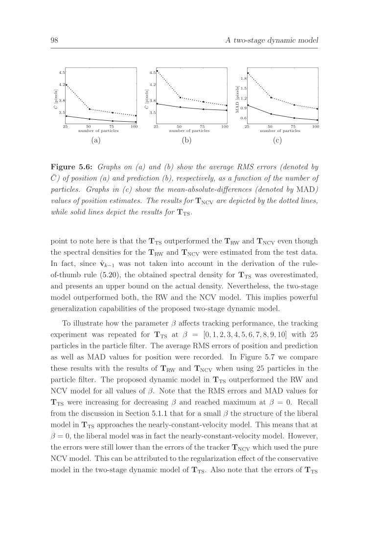
98 A two-stage dynamic model

number of particles

C[p

ixels

]

25 50 75 100

3.5

3.8

4.2

4.5

number of particles

C[p

ixels

]

25 50 75 100

3.5

3.8

4.2

4.5

number of particles

MA

D[p

ixels

]

25 50 75 100

0.6

0.9

1.2

1.5

1.8

(a) (b) (c)

Figure 5.6: Graphs on (a) and (b) show the average RMS errors (denoted by

C) of position (a) and prediction (b), respectively, as a function of the number of

particles. Graphs in (c) show the mean-absolute-differences (denoted by MAD)

values of position estimates. The results for TNCV are depicted by the dotted lines,

while solid lines depict the results for TTS.

point to note here is that the TTS outperformed the TRW and TNCV even though

the spectral densities for the TRW and TNCV were estimated from the test data.

In fact, since vk−1 was not taken into account in the derivation of the rule-

of-thumb rule (5.20), the obtained spectral density for TTS was overestimated,

and presents an upper bound on the actual density. Nevertheless, the two-stage

model outperformed both, the RW and the NCV model. This implies powerful

generalization capabilities of the proposed two-stage dynamic model.

To illustrate how the parameter β affects tracking performance, the tracking

experiment was repeated for TTS at β = [0, 1, 2, 3, 4, 5, 6, 7, 8, 9, 10] with 25

particles in the particle filter. The average RMS errors of position and prediction

as well as MAD values for position were recorded. In Figure 5.7 we compare

these results with the results of TRW and TNCV when using 25 particles in the

particle filter. The proposed dynamic model in TTS outperformed the RW and

NCV model for all values of β. Note that the RMS errors and MAD values for

TTS were increasing for decreasing β and reached maximum at β = 0. Recall

from the discussion in Section 5.1.1 that for a small β the structure of the liberal

model in TTS approaches the nearly-constant-velocity model. This means that at

β = 0, the liberal model was in fact the nearly-constant-velocity model. However,

the errors were still lower than the errors of the tracker TNCV which used the pure

NCV model. This can be attributed to the regularization effect of the conservative

model in the two-stage dynamic model of TTS. Also note that the errors of TTS

5.4 Experimental study 99

do not significantly decrease with increasing β over β = 2, which further confirms

our discussion in Section 5.1.1 on the choice of this parameter.

β

C[p

ixels

]

0 1 2 3 4 5 6 7 8 9 10

3.5

4.5

5.5

6.5

βC

[pix

els

]

0 1 2 3 4 5 6 7 8 9 103.5

4.5

5.5

6.5

7.5

β

MA

D[p

ixels

]

0 2 3 4 5 6 7 8 9 10

1

1

1.3

1.6

1.9

(a) (b) (c)

Figure 5.7: Graphs on (a) and (b) show the average RMS errors (denoted by C)

of position (a) and prediction (b), respectively, as a function of the parameter β.

Graphs in (c) show the mean-absolute-differences (denoted by MAD) of position

estimation. The results for TRW are depicted by the dashed lines, the results for

TNCV are show in dotted lines, while the solid lines depict the results for TTS.

5.4.2 Experiment 2: Tracking person’s hands

To demonstrate the generality of the proposed two-stage dynamic model, we

have revisited the experiment of tracking person’s hands from Chapter 4. There,

a person was facing the camera and waving his hands; an image of the person is

shown in Figure 5.8. Both hands were approximately 20×20 pixels large, and were

tracked with the two-stage tracker from the previous experiment. All parameters

of the tracker remained the same as in the previous experiment, except for the

spectral density qc. The spectral density was estimated using the rule-of-thumb

rule from section 5.1.2 and assuming that the expected distance that the hand

travels between two time-steps is approximately σm = 6 pixels. The number

of particles in the particle filter was set to only N = 25 particles. We denote

this tracker by TTS. For reference, the hands were also tracked using a tracker

which applied a nearly-constant-velocity (NCV) model instead of the two-stage

dynamic model and which used N = 50 particles in the particle filter; we denote

this tracker by TNCV.

The hands were tracked separately five times with TTS and TNCV, and an

average times that the tracker lost a hand was recorded. The results of tracking

100 A two-stage dynamic model

Figure 5.8: Image of a person waving his hands.

using the purely color-based model from Chapter 3 are shown in Table 5.4, while

the results for tracking with the combined visual model from Chapter 4 are shown

in Table 5.5. From Table 5.4 we see that when the purely color-based visual model

was used, TNCV lost a hand on average 26 times, while the two-stage dynamic

model in TTS reduced the number of failures to 16. We have observed a similar

reduction of failures when the combined visual model was used (Table 5.5) instead

of the purely color-based. There, the TNCV failed only four times, however, the

two-stage dynamic model in TTS was still able to reduce the number of failures

by two failures. Note also, that not only did the two-stage dynamic model reduce

the number of failures in comparison to the NCV model, but was able to do so

requiring half as many particles in the particle filter as the NCV model.

Table 5.4: Results for tracking hands using a purely color-based model from

Chapter 3

tracker dynamic model number of particles number of failures

TTS two-stage 25 16

TNCV NCV 50 26

Table 5.5: Results for tracking hands using the combined visual model from

Chapter 4

tracker dynamic model number of particles number of failures

TTS two-stage 25 2

TNCV NCV 50 4

5.5 Conclusion 101

From the results in Table 5.4 and Table 5.5 we can conclude that the two-stage

dynamic model improves tracking by reducing the number of failures, while at

the same time requiring only a small number of particles in the particle filter. We

can also conclude that the two-stage dynamic model is general enough to improve

tracking not only when tracking entire persons but also parts of persons, such as

hands.

5.5 Conclusion

In this chapter we have proposed a two-stage dynamic model and a corresponding

two-stage probabilistic tracker, which can account for various types of motions,

which we usually encounter when tracking persons. The proposed model is

composed from two separate dynamic models. The first dynamic model is

called the liberal dynamic model which was derived in Section 5.1 from a non-

zero-mean Gauss-Markov process. An analysis of the parameters of the liberal

model in Section 5.1.1 has shown that two widely-used models, the random-

walk (RW) model and the nearly-constant-velocity (NCV) model, are obtained

at the limiting values of the model’s parameters. We have also noted that the

liberal model can explain even motions which are in between the RW and the

NCV model. An important parameter of the liberal model is the spectral density

of the Gauss-Markov process, which depends on the dynamics of the class of

objects to be tracked. In Section 5.1.2 we have therefore derived a rule-of-

thumb rule to selecting this density, which requires only a vague estimate of

the target dynamics. Furthermore, by controlling the mean value of the Gauss-

Markov process, the liberal model can even further adjust to the dynamics of

the tracked target. To efficiently estimate this mean value in the liberal model,

another dynamic model, which we call the conservative model, was proposed in

Section 5.2. In contrast to the liberal model which allows greater perturbations

in target’s motion, the conservative model assumes stronger constraints on the

target velocity. In Section 5.3 we have proposed a two-stage probabilistic tracker

which uses the liberal dynamic model within a particle filter to efficiently explore

the state space of the tracked target. On the other hand, the conservative model

is used to estimate the mean value of the Gauss-Markov process in the liberal

model as well as for regularizing the estimations from the particle filter.

102 A two-stage dynamic model

Two experiments were designed to evaluate the performance of the proposed

two-stage dynamic model. The first experiment involved tracking persons running

on the path which was drawn on the floor. The path was designed such that

the observed motion included accelerations, decelerations, short runs in a certain

direction and sudden changes in the direction of motion. All persons were tracked

with the proposed dynamic model as well as with two reference trackers which

employed one of the two widely-used dynamic models – the RW model and the

NCV model. The results have shown that the proposed dynamic model performed

significantly better than the RW as well as NCV model. In particular, the two-

stage dynamic model yielded a better accuracy of tracking in comparison to

the RW and NCV models, and at the same time required significantly smaller

number of particles in the particle filter. In the second experiment we have

tracked person’s hands using the proposed dynamic model and a NCV model.

The proposed dynamic model was able to use half as many particles in the particle

filter as the NCV model while still reducing the number of times that tracking

failed in comparison to the NCV model. The results of the two experiments firstly

imply superiority of the two-stage model over the RW and NCV in accounting

for various dynamics of moving persons as well as parts of persons such as hands.

Secondly, the two-stage model allows using smaller number of particles, which can

in practice significantly reduce the computation time of a single tracking iteration

and thus makes tracking more feasible for real-time applications.

A set is a Many that allows itself to be thought of as a One.

Georg F. L. P. Cantor (1845 – 1918)

Chapter 6

Tracking multiple interacting targets

In previous chapters we have focused on deriving efficient visual and dynamic

models for tracking persons in the visual data. In this chapter we will consider

the tracking of multiple targets as a state-estimation problem, which we pose

in terms of Bayesian recursive filtering. If we assume that targets can interact,

then the state of one target at one time-step may also depend on the state of

another target at that time-step. Also, the visual data corresponding to one of

the targets may depend on other targets as well, since different constellations of

targets differently influence the visual data. We can thus think about tracking

of multiple targets as a problem of estimating the state of a complex system,

where the state of this system is exactly the constellation of all targets along

with their internal parameters (e.g., their sizes). A direct approach to solving

this problem might be to concatenate the states of all targets into a single joint-

state and apply the particle filter to recursively estimate the posterior over that

joint state. However, as we have discussed in the related work (Section 1.1.3),

this approach has several drawbacks. As it turns out, the dimensionality of

this problem increases exponentially with the number of targets considered. In

order to satisfy even a modest criteria of the estimation accuracy, the number

of particles in the particle filter needs to be increased significantly. Since the

visual model has to be calculated and compared to a reference model for each

particle, this leads to an increased expenditure of computational resources and

dramatically slows down tracking.

In this chapter we argue that, in certain applications, the context within which

the targets are observed can be used to simplify the tracking. In particular, we

will focus on applications when the camera is positioned such that the scene is

103

104 Tracking multiple interacting targets

Camera

Scene

Image

112

23

3

4

4

5 5

6 6

Figure 6.1: An example of the camera placement such that the scene is viewed

from a bird’s-eye view (left) and an example of an image from the camera (right).

The image is partitioned into several partitions, such that each partition contains

a single person. These partitions are illustrated as circular regions around the

persons.

viewed from a bird’s-eye view. We will show that in those cases a coarse model

of the target position can be derived and used to simplify the Bayesian filtering

of the targets’ joint states.

This chapter is summarized as follows. In Section 6.1 we show how the

context within which targets are viewed can be used to derive restrictions of

the targets’ positions and simplify the Bayes estimation. A parametric model of

these restrictions is given in Section 6.2 and in Section 6.3 we derive the context-

based multiple target tracking scheme. Results of the experiments are given in

Section 6.4 and in Section 6.5 we draw conclusions.

6.1 Using the physical context

In many applications, such as tracking in sports and visual surveillance, the

camera is placed such that the scene is viewed from above; see, for example,

Figure 6.1. In these situations, the objects often appear similar and their

identities cannot be maintained simply based on the visual information. Although

the motion-based visual models (e.g., the one which was proposed in Chapter 4)

may resolve some situations where visually-similar targets interact, they cannot

resolve situations in which several targets collide and stop moving, or stay

together and move as a single body.

6.2 Parametric model of partitions 105

However, we can still make use of the camera placement. While (near)

collisions among objects can be frequent, the bird’s-eye view guarantees that

complete occlusions between objects are rare. This means that we can partition

every current image into a set of partitions, such that each partition contains only

a single target (Figure 6.1b). If that is the case, then each target can be tracked

with a separate tracker only within the corresponding partition.

In Bayesian terms, the partitioning, we denote it by Vk, can be viewed as

a latent variable, which simplifies the tracking in two ways. Firstly, if we know

Vk, then the state of one target becomes independent of the states of the other

targets, since we already know that there is only a single target in each partition.

Secondly, the visual data which corresponds to one target is independent of the

other targets since it comes form a region in image which contains no other target.

Formally, we let Xk denote the joint state, i.e., the concatenation of the states(j)xk of all Np targets Xk

∆=(j)xkNp

j=1. In terms of Bayesian filtering, the aim

is to estimate the joint-state posterior p(Xk|y1:k) through time. If the current

partitioning Vk is known, the targets’ states become conditionally independent

given the partitioning. The posterior conditioned on Vk factors across all the

targets as

p(Xt|y1:k,Vk) =

Np∏

j=1

p((j)xk|y1:k,Vk), (6.1)

where p((j)xk|y1:k,Vk) is the posterior of the j-th target conditioned on the

partitioning Vk. This directly implies that the Bayes filter for the joint-state

simplifies into Np separate single-state Bayes filters, and the complexity of the

filter becomes linear with respect to the number of targets.

6.2 Parametric model of partitions

Until now we have talked about the partitioning Vk only in an abstract way.

However, to be able to efficiently implement (6.1) we require a parametric model

of the partitioning. Given a set of target positions, the parametric model has

to partition the image into a set of non-overlapping regions, such that each

region contains only a single target. One way to achieve such a partitioning

is to construct a Voronoi diagram [45] which is completely defined by the set of

points/seeds S = (j)sNp

j=1. The Voronoi diagram generates a set of Np pairwise-

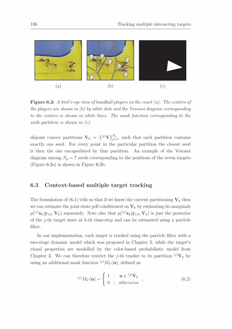
106 Tracking multiple interacting targets

s1

s2 s3

s4s5

s6

s7

(a) (b) (c)

Figure 6.2: A bird’s-eye view of handball players on the court (a). The centers of

the players are shown in (b) by white dots and the Voronoi diagram corresponding

to the centers is shown in white lines. The mask function corresponding to the

sixth partition is shown in (c).

disjoint convex partitions Vk = (j)VNp

j=1, such that each partition contains

exactly one seed. For every point in the particular partition the closest seed

is then the one encapsulated by that partition. An example of the Voronoi

diagram among Np = 7 seeds corresponding to the positions of the seven targets

(Figure 6.2a) is shown in Figure 6.2b.

6.3 Context-based multiple target tracking

The formulation of (6.1) tells us that if we know the current partitioning Vk then

we can estimate the joint-state pdf conditioned on Vk by estimating its marginals

p((j)xk|y1:k,Vk) separately. Note also that p((j)xk|y1:k,Vk) is just the posterior

of the j-th target state at k-th time-step and can be estimated using a particle

filter.

In our implementation, each target is tracked using the particle filter with a

two-stage dynamic model which was proposed in Chapter 5, while the target’s

visual properties are modelled by the color-based probabilistic model from

Chapter 3. We can therefore restrict the j-th tracker to its partition (j)Vk by

using an additional mask function (j)MV (u), defined as

(j)MV (u) =

1 ; u ∈ (j)Vk

0 ; otherwise, (6.2)

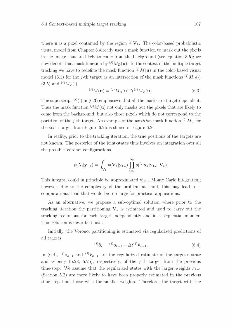
6.3 Context-based multiple target tracking 107

where u is a pixel contained by the region (j)Vk. The color-based probabilistic

visual model from Chapter 3 already uses a mask function to mask out the pixels

in the image that are likely to come from the background (see equation 3.5); we

now denote that mask function by (j)MD(u). In the context of the multiple target

tracking we have to redefine the mask function (j)M(u) in the color-based visual

model (3.1) for the j-th target as an intersection of the mask functions (j)MD(·)(3.5) and (j)MV (·)

(j)M(u) = (j)MD(u) ∩ (j)MV (u). (6.3)

The superscript (j)(·) in (6.3) emphasizes that all the masks are target-dependent.

Thus the mask function (j)M(u) not only masks out the pixels that are likely to

come from the background, but also those pixels which do not correspond to the

partition of the j-th target. An example of the partition mask function (6)MV for

the sixth target from Figure 6.2b is shown in Figure 6.2c.

In reality, prior to the tracking iteration, the true positions of the targets are

not known. The posterior of the joint-states thus involves an integration over all

the possible Voronoi configurations

p(Xt|y1:k) =

∫

Vk

p(Vk|y1:k)

Np∏

j=1

p((j)xk|y1:k,Vk).

This integral could in principle be approximated via a Monte Carlo integration;

however, due to the complexity of the problem at hand, this may lead to a

computational load that would be too large for practical applications.

As an alternative, we propose a sub-optimal solution where prior to the

tracking iteration the partitioning Vk is estimated and used to carry out the

tracking recursions for each target independently and in a sequential manner.

This solution is described next.

Initially, the Voronoi partitioning is estimated via regularized predictions of

all targets(j)ok = (j)ok−1 + ∆t(j)vk−1. (6.4)

In (6.4), (j)ok−1 and (j)vk−1 are the regularized estimate of the target’s state

and velocity (5.28, 5.25), respectively, of the j-th target from the previous

time-step. We assume that the regularized states with the larger weights πk−1

(Section 5.2) are more likely to have been properly estimated in the previous

time-step than those with the smaller weights. Therefore, the target with the

108 Tracking multiple interacting targets

largest weight πk−1 is chosen and the single-target tracking iteration is carried

out for that target using the initially estimated Voronoi partitioning. The current

regularized state of the target is then calculated and used to update the Voronoi

partitioning. Next, the target with the second-largest weight πk−1 is selected and

the procedure is repeated until all the single-target trackers are processed. A

summary of the proposed, context-based multi-target tracker for Np targets is

given in Algorithm 6.1.

In principle, the sequential recursing through single-target trackers described

above could be repeated a few times in order to arrive at a better estimation

of the current partitioning Vk. This would then lead to better estimates of the

single-target posteriors. However, in our experience, a single iteration is sufficient

to achieve satisfactory results.

6.4 Experimental study

To evaluate the effectiveness of the multi-target interaction scheme from

Section 6.3 we have compared the proposed context-based multi-target tracker

(Algorithm 6.1), we denote it by TMTT, to the so-called naive tracker, which

we denote by Tnaive. The naive tracker was conceptually equal to the proposed

TMTT, with the only difference that the Voronoi mask functions (j)MV (6.2) were

always set to unity for all the targets. Thus the tracker Tnaive was essentially

a set of color-based probabilistic trackers from Chapter 3 that did not interact

according interaction scheme from Section 6.3.

The trackers were compared by tracking players from two recordings of a

handball match and two recordings of a basketball match. Throughout the rest

of this section we will refer to the handball and the basketball recordings as

Handball1, Handball2, Basketball1 and Basketball2. A typical image from each

recording is shown in Figure 6.3.

6.4.1 Description of the recordings

Two teams, each consisting of six players, were tracked in the recordings of the

handball matches (Figure 6.3a,b). The players of one team were wearing white

shirts, and the players of the other team were wearing black shirts. The color

of the court was mainly yellow and blue, with a few advertisement stickers on

6.4 Experimental study 109

1 2

3

4 5 6

7

8

910

11

12

Handball1

1

2 3 45

67

8

9

10

11

12

Handball2

(a) (b)

1 2

3

4

5

6

7

8910

Basketball1

12

3

4

56

7

8

9

10

Basketball2

(c) (d)

Figure 6.3: Typical images from the four recordings used in the experiments for

tracking multiple persons. The first two images (a,b) show the twelve players of

a handball match, while the second two images (c,d) show the ten players of a

basketball match. All the players are depicted by a circle and a numeric label.

110 Tracking multiple interacting targets

Initialize:

• Initialize the tracker by selecting the targets. (e.g. manually)

Tracking:

• For k = 1, 2, 3, . . .

1. Sort the targets in a descending order in terms of the weights πk−1 of their

corresponding regularized states ok−1.

2. Initialize all the seeds with the predicted states (6.4):

S = (j)sNp

j=1; (j)s ← (j)ok

3. For j = 1 : Np

– Construct a set of Voronoi partitions Vk = (j)VkNp

j=1 using the set of

the current seeds S.

– Construct the Voronoi mask (j)MV (u) of the j-th target via (6.2) and

calculate the single-target mask function (j)M(u) from (6.3).

– Execute an iteration of the two-stage probabilistic tracker from

Algorithm 5.1 for the j-th target.

– Update the j-th Voronoi seed with the regularized average state of the

j-th target: (j)s ← (j)ok.

Algorithm 6.1: Context-based multiple-interacting-target tracker.

it. Because of the reflective properties of the material from which the court was

made, and because of the side effects associated with using S-VHS tape for the

video recording, the textures of the players varied significantly across different

parts of the court. For example, white players appeared yellow on the yellow

part of the court and blue on the blue part of the court. The textures of the

black players were less affected by the color of the court.

In the experiments with the basketball matches, two teams, each consisting

of five players, were tracked. In both recordings (Figure 6.3c,d) the colors of the

players were not influenced by the background as severely as they were in the

recordings of the handball. Since all four recordings were originally recorded on

an analog VHS recorder prior to digitization, they suffered from an effect called

6.4 Experimental study 111

Table 6.1: Data for the recordings used in the experiments of tracking multiple

persons

recording frame rate number of players length image size

[/s] [frames] [pixels]

Handball1 25 12 935 348×288

Handball2 25 12 1264 348×288

Basketball1 25 10 733 368×288

Basketball2 25 10 566 368×288

color bleeding. This resulted in bright colors spreading into the adjacent darker

areas. For example, in Figure 6.3a,b, the yellow patch of the court seems to be

shifted to the right by a few pixels. Further information regarding the recordings

is given in Table 6.1.

6.4.2 Results

The players were initialized manually and tracked throughout the entire

recording. When a particular player was lost, the tracker was manually

reinitialized for that player and the tracking proceeded. The number of particles

used for the tracking was 25 particles per player. In the recordings of the handball,

the widths and heights of the players’ ellipses were constrained to lie within the

interval [6,8] pixels. In the case of the basketball recordings the interval [6,10]

pixels was used. All the players were tracked five times with both trackers, and

for each repetition the number of times the tracker failed was recorded. The

results, averaged over the five repetitions, are shown in Table 6.2.

The second and the third column of Table 6.2 show the average number of

failures encountered by the trackers TMTT and Tnaive during the experiment.

These columns show that in all cases the introduction of the multi-target context

(Section 6.1) substantially reduced the number of failures and thus significantly

improved the tracking. The results of the two columns could not be compared

directly across different recordings because the recordings differed in their lengths

as well as in the number of players. For this reason the results for each experiment

were recalculated into failure rates per player and then normalized to a time-frame

of one minute. These results are shown in the last two columns of Table 6.2.

From the fourth column we see that the failure rates were approximately equal

112 Tracking multiple interacting targets

Table 6.2: The results for tracking multiple players with the proposed and the

naive multi-target tracker

average number of failures failure rate per player

[/recording] [/min]

recording Tnaive TMTT Tnaive TMTT

Handball1 28.6 3.6 3.82 0.48

Handball2 33.0 7.6 3.26 0.75

Basketball1 13.4 3.0 2.74 0.61

Basketball2 4.4 0.4 1.17 0.11The naive tracker is denoted by Tnaive, while the proposed multi-player tracker is

denoted by TMTT. The second and the third columns show the average number of

failures encountered by each tracker during the experiment. The last two columns

show the same results recalculated to represent the number of times each tracker

is expected to fail per player during one minute of tracking.

for all four experiments with the Tnaive tracker. While in comparison to Tnaive

the proposed multi-player tracker TMTT significantly reduced the failure rates,

there were still some small residual failure rates present. These varied across the

four recordings, as can be seen by comparing the results in the last column of

Table 6.2. After a further inspection of the tracking results, we concluded that

the residual failures could be assigned to one of the following four groups of errors:

1. Some of the failures arose solely due to a heavily cluttered background,

and were not caused by interactions among the neighboring players. A

substantial number of the failures in the recording Handball2 could be

attributed to the background clutter. In this match, for example, the player

with the identification number 1 (Figure 6.3b) could hardly be distinguished

from the background (see Figure 6.4).

2. Sometimes two similar players came very close to one another and were

switched by the tracker despite the use of Voronoi partitioning. Such

failures occurred only rarely, usually when just before the (near) collision

the position and prediction of at least one of the colliding players was poorly

estimated. An example of the switching of two black players in the recording

Basketball2 is shown in Figure 6.5.

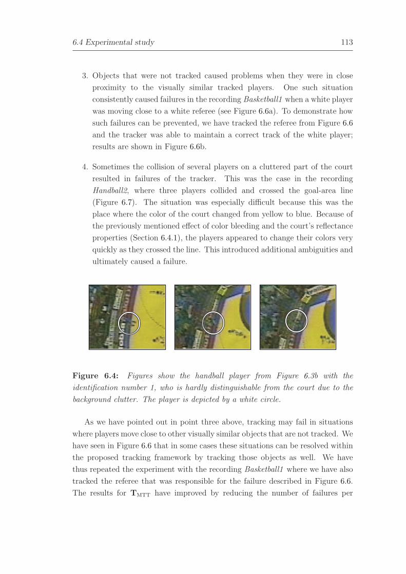
6.4 Experimental study 113

3. Objects that were not tracked caused problems when they were in close

proximity to the visually similar tracked players. One such situation

consistently caused failures in the recording Basketball1 when a white player

was moving close to a white referee (see Figure 6.6a). To demonstrate how

such failures can be prevented, we have tracked the referee from Figure 6.6

and the tracker was able to maintain a correct track of the white player;

results are shown in Figure 6.6b.

4. Sometimes the collision of several players on a cluttered part of the court

resulted in failures of the tracker. This was the case in the recording

Handball2, where three players collided and crossed the goal-area line

(Figure 6.7). The situation was especially difficult because this was the

place where the color of the court changed from yellow to blue. Because of

the previously mentioned effect of color bleeding and the court’s reflectance

properties (Section 6.4.1), the players appeared to change their colors very

quickly as they crossed the line. This introduced additional ambiguities and

ultimately caused a failure.

Figure 6.4: Figures show the handball player from Figure 6.3b with the

identification number 1, who is hardly distinguishable from the court due to the

background clutter. The player is depicted by a white circle.

As we have pointed out in point three above, tracking may fail in situations

where players move close to other visually similar objects that are not tracked. We

have seen in Figure 6.6 that in some cases these situations can be resolved within

the proposed tracking framework by tracking those objects as well. We have

thus repeated the experiment with the recording Basketball1 where we have also

tracked the referee that was responsible for the failure described in Figure 6.6.

The results for TMTT have improved by reducing the number of failures per

114 Tracking multiple interacting targets

11

22

1

1

22

1

1

2

2

Figure 6.5: Figures show two visually similar players in a basketball match

during a near collision. The players’ true identities are indicated by the numbers

in the white squares. The tracker-estimated states and the corresponding identities

are depicted by white ellipses and the Voronoi partitioning is indicated by a white

line separating the players. Note that before the collision the markers with the

same identification number denote the same players (left). Just before the players

pass by one another, the state of the player with the identification number 2 is

badly estimated (middle), and the tracker switches their identities (right).

experiment by one failure. However, in real-life there are many situations where

it is not possible or even desired to track all objects in the scene. For example,

in the field of sports analysis, sport experts are usually interested in the teams,

or a selection of players, rather than everyone on the court. We have observed

that sports experts usually track a selection of players at a time. The reason

is that switching two players, or improper tracking of a single player, could

have a devastating effect on the subsequent analysis that sports experts perform.

Therefore, situations where a player is tracked, and the referee (or even another

player) is not, are common in practice. In those situations, failures like the one

described in Figure 6.6a can be expected.

In general, the proposed, multi-target tracker TMTT exhibited a robust

performance and maintained a successful track even through the persistent

collisions of several visually similar players. A sequence of three images from

the recording Handball1 (Figure 6.8) shows an example, where several players

collide and remain in collision. The tracker TMTT successfully tracks all the

players throughout the collision while maintaining their identities.

The trackers used in the experiments were implemented in C++ and tested

on an Intel Pentium 4 personal computer with a 2.6-GHz CPU. A one time-step

iteration for tracking a single player took approximately 7 ms of processing time.

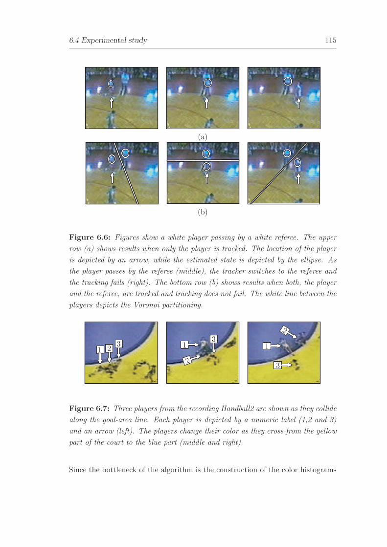
6.4 Experimental study 115

(a)

(b)

Figure 6.6: Figures show a white player passing by a white referee. The upper

row (a) shows results when only the player is tracked. The location of the player

is depicted by an arrow, while the estimated state is depicted by the ellipse. As

the player passes by the referee (middle), the tracker switches to the referee and

the tracking fails (right). The bottom row (b) shows results when both, the player

and the referee, are tracked and tracking does not fail. The white line between the

players depicts the Voronoi partitioning.

1 23 1

2

31

2

3

Figure 6.7: Three players from the recording Handball2 are shown as they collide

along the goal-area line. Each player is depicted by a numeric label (1,2 and 3)

and an arrow (left). The players change their color as they cross from the yellow

part of the court to the blue part (middle and right).

Since the bottleneck of the algorithm is the construction of the color histograms

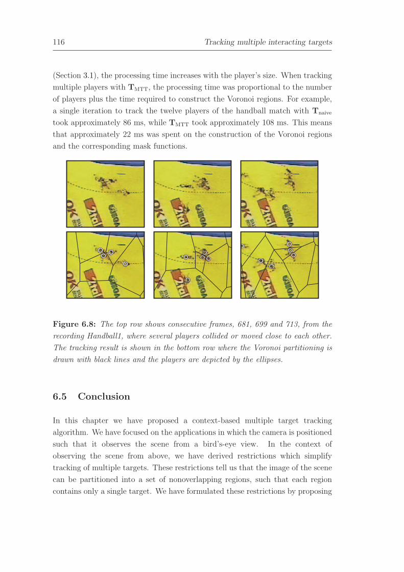
116 Tracking multiple interacting targets

(Section 3.1), the processing time increases with the player’s size. When tracking

multiple players with TMTT, the processing time was proportional to the number

of players plus the time required to construct the Voronoi regions. For example,

a single iteration to track the twelve players of the handball match with Tnaive

took approximately 86 ms, while TMTT took approximately 108 ms. This means

that approximately 22 ms was spent on the construction of the Voronoi regions

and the corresponding mask functions.

Figure 6.8: The top row shows consecutive frames, 681, 699 and 713, from the

recording Handball1, where several players collided or moved close to each other.

The tracking result is shown in the bottom row where the Voronoi partitioning is

drawn with black lines and the players are depicted by the ellipses.

6.5 Conclusion

In this chapter we have proposed a context-based multiple target tracking

algorithm. We have focused on the applications in which the camera is positioned

such that it observes the scene from a bird’s-eye view. In the context of

observing the scene from above, we have derived restrictions which simplify

tracking of multiple targets. These restrictions tell us that the image of the scene

can be partitioned into a set of nonoverlapping regions, such that each region

contains only a single target. We have formulated these restrictions by proposing

6.5 Conclusion 117

a parametric model of the image partitioning. We have proposed a scheme

to integrate the parametric model within the particle filtering framework. In

Bayesian terms, the parametric model of partitions acts as a latent variable which

simplifies the Bayes filter for tracking multiple targets and allows that each target

is tracked by a separate tracker. This significantly reduces the computational

complexity of the multiple target tracking problem. A two-stage dynamic model

from Chapter 5 is used within the particle filters for each target, which further

reduces the number of particles required for tracking and thus makes the tracker

computationally more efficient.

The proposed context-based multiple-target tracker was tested on a

demanding data-set which contained recordings of handball and basketball

matches. The tracker was compared to another, reference, tracker which was

equal to the proposed tracker in all respects, except that the reference tracker

did not make use of the partitioning model and was equal to a set of independent

single-target trackers. In all experiments, the proposed tracker outperformed the

reference tracker by significantly reducing the number of failures.

Note that the proposed context-based multiple-target tracker is a framework

of how to combine single-target trackers to approximate the joint-state Bayes

recursive filter. Thus its performance can be increased merely by replacing the

single-target particle filters with other, more advanced trackers. Furthermore, we

believe that this framework does not necessarily need to be applied in the context

of probabilistic tracking with particle filters. Other, non Bayesian, single-target

trackers may also be combined using this framework into a multiple-target tracker

to improve their performance in tracking multiple targets.

118 Tracking multiple interacting targets

I hate quotations. Tell me what you know.

Ralph W. Emerson (1803 — 1882)

Chapter 7

Conclusion

In this thesis we have focused on probabilistic models for tracking persons in visual

data. Tracking was defined within the context of probabilistic estimation, where

the parameters of the target’s model are considered random variables and the

aim is to estimate, recursively in time, the posterior probability density function

over these parameters. The recursive estimation was approached within the

established Bayesian framework of particle filtering. Several aspects of tracking

persons have been considered in this thesis: (1) how to build a reliable visual

model of a person, (2) how to efficiently model the person’s dynamics, and (3)

how to devise a scheme to track multiple persons.

One of the essential parts of visual tracking is the visual model, which allows us

to evaluate whether a person is located at a given position in the image. We have

based our visual model on color histograms and proposed several improvements

that consider tracking using the color information. The first improvement was

the color-based measure of the target’s presence that uses information from

the approximation of the background image to reduce the influence of the

background clutter. Using model-selection methodology and maximum likelihood

estimation we have then proposed the likelihood function, which can be used

to probabilistically interpret values of the proposed target’s presence measure.

However, in cases when the target is moving on those parts of the background

that are very similar to the color of the target, the proposed measure of presence

may not be discriminative enough. For that reason we have considered the

background subtraction, i.e., generating a mask function which masks out pixels

in the current image that do not belong to the target. In situations where the

lighting of the scene is changing, or the camera is moving or shaking, it is usually

119

120 Conclusion

difficult to obtain an accurate model of the background. For that reason we have

considered using only a simple approximation to the background and proposed

a dynamic background subtraction. In our implementation, the mask function is

then generated by evaluating the similarity between the tracked target and the

background model and is in that sense specialized to the tracked target. Another

improvement is the selective adaptation of the target visual model, which is used

to guard against updating the color-based visual model in situations where the

position of the target is falsely estimated or when the target is being occluded. We

have also shown how these improvements are probabilistically combined, within

the framework of particle filters, into a color-based probabilistic tracker.

Experimental results have shown that the proposed purely color-based

probabilistic visual model significantly improves tracking performance in cases

when the color of the background is similar to the color of the tracked object and

can handle short-term occlusions between visually-different objects. However, it

cannot handle situations in which the target is in a close proximity of another,

visually similar, object, or worse yet, when it is occluded by it. We have therefore

proposed to extend the purely color-based model with another model, which we

have named the local-motion model. The local-motion model is calculated from

the optical flow which we estimate using the Lucas-Kanade algorithm. While

the Lucas-Kanade algorithm is relatively fast, it gives poor estimates of the

optical flow in regions which lack texture. For that reason, we use the Shi-Tomasi

features to detect regions with enough texture and estimate the optical flow only

at those regions. Thus the local-motion is defined using only a sparse optical

flow. To account for the errors in the optical flow estimation and rapid changes

in the target’s motion, we have derived a probabilistic model of the local-motion.

Since the local-motion model significantly varies during target’s movement, an

adaptation scheme for the local-motion model was devised. The proposed local-

motion model is probabilistically combined with the color-based model into a

combined visual model and we have proposed a particle-filter-based tracker which

uses this model. Experiments have shown that the proposed combined visual

model is able to resolve occlusions between visually-similar objects. We have

demonstrated these improvements with examples of tracking person’s palms, as

well as tracking persons in surveillance and in a sports match.

We have then focused on another essential part of a probabilistic tracker,

the dynamic model, by which we describe the dynamics of the tracked target.

121

We have proposed a two-stage dynamic model, and a corresponding two-stage

probabilistic tracker, which can account for various types of motions that are

characteristic for a moving person. The proposed model is composed of two

separate dynamic models. The first dynamic model is called the liberal dynamic

model and was derived from a non-zero-mean Gauss-Markov process. An analysis

of the parameters of the liberal model has shown that two widely-used models,

the random-walk (RW) model and the nearly-constant-velocity (NCV) model,

are obtained at the limiting values of the model’s parameters. We have also

noted that the liberal model can explain even motions which are in between the

RW and the NCV model. An important parameter of the liberal model is the

spectral density of the Gauss-Markov process, which depends on the dynamics

of the class of objects to be tracked. We have therefore derived a rule-of-thumb

rule to selecting this density, which requires only a vague estimate of the target

dynamics. Furthermore, by controlling the mean value of the Gauss-Markov

process, the liberal model can even further adjust to the dynamics of the tracked

target. To efficiently estimate this mean value in the liberal model, another

dynamic model, which we call the conservative model, was proposed. In contrast

to the liberal model, which allows larger perturbations in target’s motion, the

conservative model assumes stronger constraints on the target’s velocity. The

proposed two-stage probabilistic tracker uses the liberal dynamic model within

a particle filter to efficiently explore the state space of the tracked target. On

the other hand, the conservative model is used to estimate the mean value of

the Gauss-Markov process in the liberal model, as well as for regularizing the

estimations from the particle filter. Experiments have shown that, when used in a

particle filter, the proposed dynamic model outperforms the widely-used dynamic

models by reducing the number of times a target is lost and achieving a better

accuracy of target’s position and prediction. The proposed two-stage dynamic

model also allows using a smaller number of particles in the particle filter, which

significantly reduces the processing time required for a single tracking iteration.

In the last part of the thesis we have considered extending the proposed

solutions for single-target tracking to the problem of tracking multiple persons.

We have focused on applications in which the camera observes the scene from

a bird’s-eye view, and proposed a novel context-based multiple-target tracking

algorithm. In the context of observing the scene from above, we have derived

restrictions which simplify the tracking of multiple targets. These restrictions

122 Conclusion

tell us that the image of the observed scene can be partitioned into a set of

nonoverlapping regions, such that each region includes only a single target.

We have formulated these restrictions by proposing a parametric model of the

image partitioning. We have proposed a scheme to integrate the parametric

model within the particle filtering framework. In Bayesian terms, the parametric

model of partitions acts as a latent variable which simplifies the Bayes filter for

multiple target tracking and allows tracking each target with a separate tracker.

This significantly reduces the computational complexity of the multiple target

tracking problem. The previously proposed two-stage dynamic model is used

within the particle filter for each target, which further reduces the number of

particles required for tracking and makes the tracker more efficient in terms of the

processing time. The proposed context-based multiple-target tracker was tested

on a demanding data-set which contained recordings of handball and basketball

matches. The tracker was compared to another, reference, tracker which was

equal to the proposed tracker in all respects, except that the reference tracker

did not make use of the partitioning model and was equal to a set of independent

single-target trackers. In all experiments, the proposed tracker outperformed the

reference tracker by significantly reducing the number of failures.

The solutions which were proposed in this thesis allow accurate tracking while

at the same time do not significantly increase the processing time. As such they

are ideal for use in applications like surveillance and analysis in sports. Indeed,

some of the solutions have already been integrated in an application for analysis

of performance of athletes in indoor sports like squash, tennis, basketball and

handball [110]. This application has been successfully used by sport experts from

the University of Ljubljana and the Ruhr University of Bochum to produce an

analysis of players’ motion during tennis, basketball and handball.

7.1 Summary of contributions

The contributions of the thesis are summarized below:

• A color-based visual model for tracking persons is derived, which

improves tracking in situations when the color of the tracked

object is similar to the color of the background.

Partially published in [89, 90, 92, 91].

7.2 Future work 123

• A combined visual model is proposed, which fuses the color

information with the features of local motion, to resolve occlusions

between visually similar objects.

Partially published in [88], another paper currently under submission.

• A two-stage dynamic model is proposed, which combines the

liberal and the conservative model to better describe the target’s

motion, and a method for setting the parameters of the model is

derived.

Partially published in [87].

• A context-based scheme for tracking multiple targets is proposed,

which allows tracking with a linear computational complexity.

Published in [91].

7.2 Future work

While the proposed solutions and models perform well under a variety of

demanding conditions there are still some points which could be improved. The

form of the color-based visual model was chosen to be very general to allow

tracking entire persons as well as parts of persons (hands). The model could

be further improved by accounting for the structure of the target as well. For

example, the visual model could be comprised of multiple (loosely or rigidly)

connected separate visual models. This would improve tracking in situations

where, for example, the color of the person’s upper part is significantly different

from the lower part. Perhaps the structure of these connected appearance models

could be relaxed even further – however, care should be taken not to decrease

the robustness of the color-based model. While better color-based model could

improve tracking to some extent, it would likely still suffer from the drawbacks of

the color-based visual model. Namely, it would still not be able to discriminate

between two visually similar objects. We have shown that the proposed combined

visual model offers a marked improvement when tracking visually similar objects

through occlusions. However, this model still suffers from one drawback. If

the visually similar objects move in the same way, then the model still cannot

distinguish between them and tracking fails. Also, if the tracked object drastically

changes the direction of motion during the occlusion, the local-motion model

124 Conclusion

will not be able to detect that, and tracking will fail. In situations, where the

camera is placed such that it observes the scene from above, we can resolve the

situations where visually similar objects collide and move similarly by applying

the proposed context-based multi-target tracker. However, we have still observed

some situations, where the partitioning is falsely estimated and the tracking fails.

Therefore, a method to automatically recover tracking once a target has been lost

and to detect targets as they enter the scene is still required. This is indeed a

difficult problem in its own right and will be the focus of further research. Note

that from the point of detecting the object onward, the solutions which have been

proposed in this thesis can be used directly with no, or only minor, modifications.

References

[1] A. Agarwal and B. Triggs. Tracking articulated motion with piecewise

learned dynamical models. In Proc. European Conf. Computer Vision,

2004.

[2] J. K. Aggarwal and Q. Cai. Human motion analysis: A review. Comp. Vis.

Image Understanding, 73(3):428–440, 1999.

[3] H. Akaike. A new look at the statistical model identification. IEEE Trans.

Automatic Control, 19:716–723, December 1974.

[4] D. L. Alspach and H. W. Sorenson. Nonlinear Bayesian estimation using

Gaussian sum approximation. IEEE Trans. Automatic Control, 20:439–447,

1972.

[5] B. D. O. Anderson and J. B. Moore. Optimal Filtering. New Jersy:

Prentice-Hall inc., 1979.

[6] M. Arulampalam, S. Maskell, N. Gordon, and T. Clapp. A tutorial on

particle filters for online nonlinear/non-gaussian Bayesian tracking. IEEE

Trans. Signal Proc., 50(2):174–188, February 2002.

[7] R. V. Babu, P. Perez, and P. Bouthemy. Robust tracking with motion

estimation and local kernel-based color modeling. Image and Vision

Computing, 25(8):1205–1216, August 2007.

[8] J. Bangsbo. The physiology of soccer: With special reference to intense

intermittent exercise. Acta Physiologica Scandinavica, 619:1–155, 1994.

[9] Y. Bar-Shalom, editor. Multitarget/Multisensor Tracking: Applications and

Advances, volume 2. YBS Publishing, 1998.

125

126 References

[10] Y. Bar-Shalom, X. R. Li, and T. Kirubarajan. Estimation with Applications

to Tracking and Navigation, chapter 11, pages 438–440. John Wiley & Sons,

Inc., 2001.

[11] M. Basseville. Distance measures for signal processing and pattern

recognition. Signal Processing, 18(4):349–454, 1989.

[12] A. Baumberg and D. Hogg. An efficient method for contour tracking using

active shape models. In Proc. IEEE Workshop on Motion of Non-rigid and

Articulated Objects, pages 194–199, 1994.

[13] N. Bergman. Recursive Bayesian Estimation: Navigation and Tracking

Applications. PhD thesis, Linkoping University, 1999.

[14] S. T. Birchfield and S. Rangarajan. Spatiograms versus histograms for

region-based tracking. In Proc. Conf. Comp. Vis. Pattern Recognition,

volume 2, pages 1158–1163, 2005.

[15] C. M. Bishop. Pattern Recognition and Machine Learning. Information

Science and Statistics. Springer Science+Business Media, LCC, 2006.

[16] M. J. Black and P. Anadan. The robust estimation of multiple

motions: Parametric and piecewise-smooth flow fileds. Comp. Vis. Image

Understanding, 63:75–104, 1996.

[17] M. J. Black and D. J. Fleet. Probabilistic detection and tracking of motion

discontinuities. In Proc. Int. Conf. Computer Vision, volume 1, pages 551–

558, 1999.

[18] M.J. Black. Robust dense optical flow.

http://sca2002.cs.brown.edu/∼black/ignc.html.

last visited on 21. december, 2006.

[19] A. Blake and M. Isard. Active Contours: The Application of Techniques

from Graphics,Vision,Control Theory and Statistics to Visual Tracking of

Shapes in Motion. Springer-Verlag New York, Inc., Secaucus, NJ, USA,

1998.

[20] H. A. P. Blom and E. A. Bloem. Exact bayesian and particle filtering of

stochastic hybrid systems. IEEE Trans. Aerospace and Electronic Systems,

43(1):55–70, 2006.

References 127

[21] M. Bon, J. Pers, M. Sibila, and S. Kovacic. Analiza gibanja igralca med

tekmo. Faculty of Sport, University of Ljubljana, 2001.

[22] J. Y. Bouguet. Pyramidal implementation of the lucas kanade

feature tracker: Description of the algorithm. Technical report,

Intel Corporation, Microprocessor Research Labs, last visit: 2007.

http://www.intel.com/research/mrl/research/opencv/.

[23] K. J. Bradshaw, I. D. Reid, and D. W. Murray. The active recovery of 3d

motion trajectories and their use in prediction. IEEE Trans. Patter. Anal.

Mach. Intell., 19(3):219–234, 1997.

[24] P. Brasnett, L. Mihaylova, D. Bull, and N. Canagarajah. Sequential Monte

Carlo tracking by fusing multiple cues in video sequences. Image and Vision

Computing, 25(8):1217–1227, August 2007.

[25] G. J. Brostow and R. Cipolla. Unsupervised bayesian detection of

independent motion in crowds. In Proc. Conf. Comp. Vis. Pattern

Recognition, pages I: 594–601, 2006.

[26] R. G. Brown and P. Y. C. Hwang. Introduction to Random Signals and

Applied Kalman Filtering. John Wiley & Sons, 1997.

[27] R. S. Bucy and H. M. Youssef. Nonlinear filter representation via spline

functions. In Symposium on Nonlinear Estimation, pages 51–60, 1974.

[28] A. Bugeau and P. Perez. Detection and segmentation of moving objects

in highly dynamic scenes. In Proc. Conf. Comp. Vis. Pattern Recognition,

pages 1 – 8, 2007.

[29] K. P. Burnham and D. R. Anderson. Multimodel inference: Understanding

aic and bic in model selection. Sociological Methods and Research,

33(2):261–304, 2004.

[30] Y. Cai, N. de Feritas, and J. J. Little. Robust visual tracking for multiple

targets. In Proc. European Conf. Computer Vision, volume IV, pages 107–

118, 2006.

[31] J. Carpenter, P. Clifford, and P. Fearnhead. Improved particle filter

for nonlinear problems. IEE Proceedings Radar, Sonar and Navigation,

146(1):2–7, 1999.

128 References

[32] C. Chang, R. Ansari, and A. Khokhar. Multiple object tracking with kernel

particle filter. In Proc. Conf. Comp. Vis. Pattern Recognition, volume 1,

pages 566– 573, 2005.

[33] Z. Chen. Bayesian filtering: From Kalman filters to particle filters,

and beyond. Technical report, McMaster University, Hamilton, Ontario,

Canada, 2003.

[34] K. Choi, Y. D. Seo, and S. W. Lee. Probabilistic tracking of soccer players

and ball. Proc. Asian Conf. Computer Vision, 1:27–30, January 2004.

[35] V. D. Comaniciu and P. Meer. Kernel-based object tracking. IEEE Trans.

Patter. Anal. Mach. Intell., 25(5):564–575, May 2003.

[36] T. F. Cootes and C. J. Taylor. Active shape models – ’smart snakes’. In

Proc. British Machine Vision Conference, pages 266–275, 1992.

[37] T. F. Cootes, C. J. Taylor, D. H. Cooper, and J. Graham. Training

models of shape from sets of examples. In Proc. British Machine Vision

Conference, pages 9–18, 1992.

[38] D. Cremers. Dynamical statistical shape priors for level set-based tracking.

IEEE Trans. Patter. Anal. Mach. Intell., 28(8):1262– 1273, 2006.

[39] J. Czyz, B. Ristic, and B. Macq. A color-based particle filter for joint

detection and tracking of multiple objects. In Proc. Int. Conf. Acoustics,

Speech and Signal Processing, March 2005.

[40] N. Dalal and B. Triggs. Histograms of oriented gradients for human

detection. In Proc. Conf. Comp. Vis. Pattern Recognition, volume 1, pages

886–893, June 2005.

[41] J. Deutscher, A. Blake, and I. Reid. Articulated body motion capture by

annealed particle filtering. In Proc. Conf. Comp. Vis. Pattern Recognition,

volume 2, pages 126 – 133, 2000.

[42] M. Dimitrijevic, V. Lepetit, and P. Fua. Human body pose detection using

bayesian spatio-temporal templates. Comp. Vis. Image Understanding,

104(2):127 – 139, 2006.

References 129

[43] A. Doucet, N. de Freitas, and N. Gordon, editors. Sequential Monte Carlo

Methods in Practice. New York: Springer-Verlag, January 2001.

[44] W. Du and J. H. Piater. Tracking by cluster analysis of feature points using

a mixture particle filter. In Advanced Video and Signal Based Surveillance,

pages 165– 170, 2005.

[45] R. O. Duda, P. E. Hart, and D. G. Stork. Pattern Classification, chapter

Nonparametric Techniques, pages 177–178. Wiley-Interscience Publication,

2nd edition, 2000.

[46] W. S. Erdmann. Gathering of kinematic data of sport event by televising

the whole pitch and track. In Proc. Int. Soc. Biomech. Sports Sympossium,

pages 159–162, 1992.

[47] P. Fearnhead. Sequential Monte Carlo methods in filter theory. PhD thesis,

Merton College, 1998.

[48] A. Fossati, M. Dimitrijevic, V. Lepetit, and P. Fua. Bridging the gap

between detection and tracking for 3d monocular video-based motion

capture. In Proc. Conf. Comp. Vis. Pattern Recognition, pages 1–8, 2007.

[49] P. Gabriel, J. Verly, J. Piater, and A. Genon. The state of the art in multiple

object tracking under occlusion in video sequences. In Proc. Advanced

Concepts for Intelligent Vision Systems, page 166–173, 2003.

[50] A. Galata, N. Johnson, and D. Hogg. Learning variable length markov

models of behaviour. Comp. Vis. Image Understanding, 81(3):398–413,

2001.

[51] D. M. Gavrila. The visual analysis of human movement: A survey. Comp.

Vis. Image Understanding, 73(1):82–98, 1999.

[52] J. J. Gonzalez, Lim Ik Soo, P. Fua, and D. Thalmann. Robust tracking and

segmentation of human motion in an image sequence. In Proc. IEEE Int.

Conf. Acoust., Speech, Signal Processing, volume 3, pages 29–32, 2003.

[53] N. J. Gordon, D. J. Salmond, and A. F. M. Smith. Novel approach to

nonlinear/non-gaussian Bayesian state estimation. In IEE Proc. Radar and

Signal Processing, volume 40, pages 107–113, 1993.

130 References

[54] H. Grabner, M. Grabner, and H. Bischof. Real-time tracking via on-line

boosting. In Proc. British Machine Vision Conference, pages 47–56, 2006.

[55] B. Han and L. S. Davis. Robust observations for object tracking. In Proc.

IEEE Int. Conf. Image Processing, volume 2, pages 442–445, 2005.

[56] R. Hemlick. Multitarget-Multisensor Tracking: Applications and

Advances, volume 3, chapter IMM Estimator with nearest-neighbour Joint

Probabilistic Data Association, pages 175–178. Artech House, inc., 2000.

[57] S. M. Herman. A particle filter approach to joint passive radar tracking and

target classification. PhD thesis, University of Illinois, 2002.

[58] B. K. P. Horn and B. G. Schnuck. Determining optical flow. Technical

report, Massachusetts Institute of Technology, 1980.

[59] K. Hotta. Adaptive weighting of local classifiers by particle filter. In

International Conference on Pattern Recognition, volume 2, pages 610–613,

2006.

[60] W. Hu, T. Tan, L. Wang, and Maybank S. A survey on visual surveillance

of object motion and behaviors. IEEE Transactions on Systems, Man and

Cybernetics, Part C: Applications and Reviews, 34(3):334–352, 2004.

[61] C. Hue, J. P. Le Cadre, and P. Perez. A particle filter to track multiple

objects. In IEEE Workshop on Multi-Object Tracking, pages 61–68,

Vancouver, Canada, July 2001.

[62] S. S. Intille and A. F. Bobick. Visual tracking using closed-worlds. In Proc.

Int. Conf. Computer Vision, pages 672–678, June 1995.

[63] M. Isard and A. Blake. Contour tracking by stochastic propagation of

conditional density. In Proc. European Conf. Computer Vision, volume 1,

pages 343–356, 1996.

[64] M. Isard and A. Blake. Condensation – conditional density propagation

for visual tracking. Int. J. Comput. Vision, 29(1):5–28, 1998.

[65] M. Isard and J. MacCormick. Bramble: A Bayesian multiple-blob tracker.

In Proc. Int. Conf. Computer Vision, pages 34–41, 2001.

References 131

[66] S. Iwase and H. Saito. Parallel tracking of all soccer players by integrating

detected positions in multiple view images. In International Conference on

Pattern Recognition, volume 4, pages 751–754, 2004.

[67] A. H. Jazwinski. Stochastic Processes and Filtering Theory. New York:

Academic Press, 1970.

[68] A. Jepson, D. J. Fleet, and T. El-Maraghi. Robust on-line appearance

models for vision tracking. IEEE Trans. Patter. Anal. Mach. Intell.,

25(10):1296–1311, 2003.

[69] S. Julier and J. Uhlmann. A general method for approximating nonlinear

transformations of probability distributions. Technical report, Department

of Engineering Science, University of Oxford, 1996.

[70] S. Julier and J. Uhlmann. A new extension of the kalman filter to nonlinear

systems. In International Symp. on Aerospace/Defence Sensing, Simulation

and Control, page 21–24, 1997.

[71] S. J. Julier and J. K. Uhlmann. A consistent, debiased method for

converting between polar and cartesian coordinate systems. In Proceedings

of AeroSense: The 11th International Symposium on Aerospace/Defense

Sensing, Simulation and Control, 1997.

[72] S.J. Julier. The scaled unscented transformation. volume 6, pages 4555–

4559, 2002.

[73] I. Kailath. Lecture on Wiener and Kalman Filtering. New York: Springer-

Verlag, 1980.

[74] T. Kailath. The divergence and bhattacharyya distance measures in signal

selection. IEEE Trans. Communications Technology, 15(1):52–60, 1967.

[75] T. Kailath. The innovations approach to detection and estimation theory.

In Proc. of the IEEE, volume 58, pages 680–695, 1970.

[76] R. E. Kalman. A new approach to linear filtering and prediction problems.

Trans. ASME, J. Basic Engineering, 82:34–45, 1960.

[77] J. Kang, I. Cohen, and G. Medioni. Soccer player tracking across

uncalibrated camera streams. In IEEE Int. Workshop on Visual

132 References

Surveillance and Performance Evaluation of Tracking and Surveillance In

conjunction with ICCV03, pages 172–179, 2003.

[78] J. Kang, I. Cohen, and G. Medioni. Persistent objects tracking across

multiple non-overlapping cameras. In Workshop on Motion and Video

Computing, 2005.

[79] K. Kazufumi, I. Xiong. Gaussian filters for nonlinear filtering problems.

IEEE Trans. Automatic Control, 45(5):910–927, 2000.

[80] S. Khan and M. Shah. Tracking people in presence of occlusion. In Asian

Conference on Computer Vision, 2000.

[81] Z. Khan, T. Balch, and F. Dellaert. MCMC-based particle filter for tracking

a variable number of interacting targets. IEEE Trans. Patter. Anal. Mach.

Intell., 27(11):1805–1819, November 2005.

[82] G. Kitagawa. Non-gaussian state-space modelling of nonstationary time

series. J. Amer. Stat. Assoc., 82:1032–1063, 1987.

[83] G. Kitagawa. Monte carlo filter and smoother for non-gaussian non-linear

state space models. J. Comp. and Graph. Statistics, 5(1):1–25, 1996.

[84] B. Klaus and P. Horn. Robot Vision. The MIT press, Boston, 1986.

[85] C. Kotzamanidis, K. Chatyikoloutas, and A. Gianakos. Optimization of

the training plan of the handball game. Handball: periodical for coaches,

referees and lecturers, 2:65–71, 1999.

[86] S. C. Kramer and H. W. Sorenson. Recursive Bayesian estimation using

piece-wise constant approximations. Automatica, 24(6):789–801, 1988.

[87] M. Kristan, J. Pers, A. Leonardis, and S. Kovacic. A hierarchical dynamic

model for tracking in sports. In Proceedings of the sixteen Electrotechnical

and Computer Science Conference, ERK07, September 2007.

[88] M. Kristan, J. Pers, A. Leonardis, and S. Kovacic. Probabilistic tracking

using optical flow to resolve color ambiguities. In Helmut Grabner

Michael Grabner, editor, Computer Vision Winter Workshop 2007, pages

3–10, 2007.

References 133

[89] M. Kristan, J. Pers, M. Perse, M. Bon, and S. Kovacic. Multiple interacting

targets tracking with application to team sports. In International

Symposium on Image and Signal Processing and Analysis, pages 322–327,

September 2005.

[90] M. Kristan, J. Pers, M. Perse, and S. Kovacic. Towards fast and efficient

methods for tracking players in sports. In ECCV Workshop on Computer

Vision Based Analysis in Sport Environments, pages 14–25, May 2006.

[91] M. Kristan, J. Pers, M. Perse, and S. Kovacic. Closed-world tracking

of multiple interacting targets for indoor-sports applications. Computer

Vision and Image Understanding, 2008. in press.

[92] M. Kristan, M. Perse, S. Kovacic, and J. Pers. Sledenje vec igralcev v

sportnih igrah na podlagi vizualne informacije. Electrotechnical Review,

74(1-2):19–24, May 2007.

[93] S. Kullback and R. A. Lieber. On information and sufficiency. Annals of

Mathemathical Statistics, 22:679–86, 1951.

[94] T. Lefebvre, H. Bruyninckx, and J. De Schutter. Comment on ’a new

method for the nonlinear transformations on means and covariances in

filters and estimators’. IEEE Trans. Automatic Control, 47(8):1406–1409,

2002.

[95] B. Leibe, A. Leonardis, and B. Schiele. Combined object categorization

and segmentation with an implicit shape model. In Proc. European Conf.

Computer Vision, 2004.

[96] B. Leibe, E. Seemann, and B. Schiele. Pedestrian detection in crowded

scenes. In Proc. Conf. Comp. Vis. Pattern Recognition, pages I: 878–885,

2005.

[97] P.H. Li and F. Chaumette. Image cues fusion for object tracking based on

particle filter. In Intl. Conf. Articulated Motion And Deformable Objects,

pages 99–107, 2004.

[98] W. R. Li and Y. Bar-Shalom. Performance prediction of the interacting

multiple model algorithm. IEEE Trans. Aerospace and Electronic Systems,

29(3):755–771, 1993.

134 References

[99] Y. Li and H.Z. Ai. Fast detection of independent motion in crowds

guided by supervised learning. In Proc. IEEE Int. Conf. Image Processing,

volume 3, pages 341–344, 2007.

[100] H. Lim, V. I. Morariu, O. I. Camps, and M. Sznaier. Dynamic appearance

modeling for human tracking. In Proc. Conf. Comp. Vis. Pattern

Recognition, 2006.

[101] J. S. Liu and R. Chen. Sequential monte carlo methods for dynamical

systems. J. Amer. Stat. Assoc., 93:1032–1044, 1998.

[102] W. L. Lu and J. J. Little. Tracking and recognizing actions at a distance. In

Proc. Workshop on Compter Vision Based Analisys in Sport Environments

In conjunction with ECCV06, pages 49–60, May 2006.

[103] B. D. Lucas and T. Kanade. An iterative image registration technique with

an application to stereo vision. In Imaging Understanding Workshop, pages

121–130, 1981.

[104] M. Lucena, J. M. Fuertes, and N. P. de la Blanca. Evaluation of

three optical flow-based observation models for tracking. In International

Conference on Pattern Recognition, volume 4, pages 236– 239, 2004.

[105] M. J. Lucena, J. M. Fuertes, J. I. Gomez, N. Perez de la Blanca, and

A. Garrido. Tracking from optical flow. In International Symposium on

Image and Signal Processing and Analysis, volume 2, pages 651 – 655,

2003.

[106] J. MacCormick. Probabilistic modelling and stochastic algorithms for visual

localisation and tracking. PhD thesis, University of Oxford, 2000.

[107] J. MacCormick and A. Blake. Probabilistic exclusion and partitioned

sampling for multiple object tracking. Int. J. Comput. Vision, 39(1):57–71,

2000.

[108] R. Malladi, J. A. Sethian, and B. C. Vemuri. Shape modelling with front

propagation: A level set approach. IEEE Trans. Patter. Anal. Mach.

Intell., 17(2):158–175, 1995.

References 135

[109] T. Mauthner and H. Bischof. A robust multiple object tracking for

sport applications. In Performance Evaluation for Computer Vision, 31st

AAPR/OAGM Workshop 2007, pages 81–89, May 2007.

[110] Machine Vision Group, Faculty of Electrical Engineering, University of

Ljubljana. ISAA. http://vision.fe.uni-lj.si/research/SportA/application.html.

last visited on 29 January 2008.

[111] S. McGinnity and G.W. Irwin. Multiple model bootstrap filter for

maneuvering target tracking. IEEE Trans. Aerospace and Electronic

Systems, 36(3):1006–1012, 2000.

[112] S. J. McKenna, Raja Y., and S. Gong. Object tracking using adaptive color

mixture models. In Proc. Asian Conf. Computer Vision, page 607–614,

1998.

[113] A. S. Micilotta, E. J. Ong, and R. Bowden. Detection and tracking of

humans by probabilistic body part assembly. In Proc. British Machine

Vision Conference, 2005.

[114] T. B. Moeslund and E. Granum. A survey of computer vision-based human

motion capture. Comp. Vis. Image Understanding, 81(3):231–268, March

2001.

[115] T.B. Moeslund, A. Hilton, and V. Kruger. A survey of advances in

vision-based human motion capture and analysis. Comp. Vis. Image

Understanding, 103(2-3):90–126, November 2006.

[116] C. J. Needham. Tracking and Modelling of Team Game Interactions. PhD

thesis, School of Computing, The University of Leeds, October 2003.

[117] N. Nørgraad, N. Poulsen, and O. Ravn. New developments in state

estimation for nonlinear systems. Automatica, 36(11):1627–1638, 2000.

[118] K. Nummiaro, E. Koller-Meier, and L. Van Gool. Color features for tracking

non-rigid objects. Chinese J. Automation, 29(3):345–355, May 2003.

[119] H. Ok, Y. Seo, and K. Hong. Multiple soccer players tracking by

condensation with occlusion alarm probability. In Int. Workshop on

Statistically Motivated Vision Processing, 2002.

136 References

[120] K. Okuma, A. Taleghani, N. De Freitas, J. J. Little, and D. G. Lowe.

A boosted particle filter: Multitarget detection and tracking. In Proc.

European Conf. Computer Vision, volume 1, pages 28–39, 2004.

[121] C. F. Olson and D. P. Huttenlocher. Automatic target recognition by

matching oriented edge pixels. IEEE Trans. Image Proc., 6(1):103–113,

January 1997.

[122] OpenCV. Lucas-Kanade optical flow calculation. OpenCV C++ library.

[123] P. Perez, C. Hue, J. Vermaak, and M. Gangnet. Color-based probabilistic

tracking. In Proc. European Conf. Computer Vision, volume 1, pages 661–

675, 2002.

[124] P. Perez, J. Vermaak, and A. Blake. Data fusion for visual tracking with

particles. Proc. of the IEEE, 92(3):495–513, 2004.

[125] J. Pers and S. Kovacic. Tracking people in sport : Making use of partially

controlled environment. In Int. Conf. Computer Analysis of Images and

Patterns, pages 374–382, 2001.

[126] V. Peterka. Trends and Progress in System Identification, chapter Bayesian

approach to system identification, pages 239–304. Pergamon Press, 1981.

[127] PETS: Performance Evaluation of Tracking and Surveillance. Online

database. http://www.cvg.rdg.ac.uk/slides/pets.html, 2006. last visited:

4.4.2007.

[128] F. Pitie, S. A. Berrani, A. Kokaram, and R. Dahyot. Off-line multiple object

tracking using candidate selection and the viterbi algorithm. In Proc. IEEE

Int. Conf. Image Processing, volume 3, pages 109–112, 2005.

[129] M. K. Pitt and N. Sheppard. Filtering via simulation: Auxiliary particle

filters. J. Amer. Stat. Assoc., 94(446):590–599, 1999.

[130] S. Pundlik and S. Birchfield. Motion segmentation at any speed. In Proc.

British Machine Vision Conference, volume I, pages 427–436, 2006.

[131] D. Ramanan, D. A. Forsyth, and A. Zisserman. Tracking people by learning

their appearance. IEEE Trans. Patter. Anal. Mach. Intell., 29(1):65–81,

2007.

References 137

[132] C. Rasmussen and G. D. Hager. Probabilistic data association methods for

tracking complex visual objects. IEEE Trans. Patter. Anal. Mach. Intell.,

23(6):560–576, 2001.

[133] I. Rhodes. A tutorial introduction to estimation and filtering. IEEE Trans.

Automatic Control, 16(6):688–706, 1971.

[134] B. Ripley. Stochastic Simulation. Wiley, New York, 1987.

[135] J. Rissanen. Hypothesis selection and testing by the MDL principle. Comp.

Journal, 42(4):260–269, 1999.

[136] X. Rong Li and V. Jilkov P. Survey of maneuvering target tracking:

Dynamic models. IEEE Trans. Aerospace and Electronic Systems,

39(4):1333–1363, October 2003.

[137] N. Saito and R.R. Coifman. Improved local discriminant bases using

empirical probability density estimation. In Comput. Section of American

Statistical Association, pages 312–321, 1997.

[138] D. Schulz, W. Burgard, D. Fox, and A. B. Cremers. Tracking multiple

moving targets with a mobile robot using particle filters and statistical data

association. In Proc. IEEE Int. Conf. Robotics and Automation, volume 1,

pages 665–670, 2001.

[139] G. Schwarz. Estimating the dimension of a model. Annaly of Statistics,

6(2):461–464, 1978.

[140] D. W. Scott. Multivariate Density Estimation. New York: Wiley, 1992.

[141] A. Senior. Tracking people with probabilistic appearance models. In Perf.

Eval. Track. and Surveillance in conjunction with ECCV02, pages 48–55,

2002.

[142] Y. Seo, S. Choi, H. Kim, and K. S. Hong. Where are the ball and players?

soccer game analysis with color based tracking and image mosaick. In Proc.

Int. Conf. Image Analysis and Processing, volume 2, pages 196–203, 1997.

[143] J. Shi and C. Tomasi. Good features to track. In Proc. Conf. Comp. Vis.

Pattern Recognition, pages 593 – 600, June 1994.

138 References

[144] H. Sidenbladh and M. J. Black. Learning image statistics for bayesian

tracking. In Proc. Int. Conf. Computer Vision, 2001.

[145] H. Sidenbladh, M. J. Black, and L. Sigal. Implicit probabilistic models

of human motion for synthesis and tracking. In Proc. European Conf.

Computer Vision, 2002.

[146] R. A. Singer. Estimating optimal tracking filter performance for manned

maneuvering targets. IEEE Trans. Aerospace and Electronic Systems, AES-

6(4):473–483, 1970.

[147] R. A. Singer and K. W. Benhke. Real-time tracking filter evaluation and

selection for tactical applications. IEEE Trans. Aerospace and Electronic

Systems, AES-7(1):100 – 110, 1971.

[148] M. Sonka, V. Hlavac, and R. Boyle. Image Processing, Analysis, and

Machine Learning. PWS Publishing, 1999.

[149] H. W. Sorenson. Bayesian analysis of time series and dynamic models,

chapter Recursive estimation for nonlinear dynamic systems. Dekker, 1988.

[150] H. W. Sorenson and D. L. Alspach. Recursive Bayesian estimation using

Gaussian sums. Automatica, 7(4):465–479, 1971.

[151] F. R. Stengel. Optimal Control and Estimation. Dover publications, inc.,

NY, 1994.

[152] B. Stenger, A. Thayananthan, P. H. S. Torr, and R. Cipolla. Model-based

hand tracking using a hierarchical bayesian filter. IEEE Trans. Patter.

Anal. Mach. Intell., 28(9):1372– 1384, 2006.

[153] M. J. Swain and D. H. Ballard. Colour indexing. Int. J. Comput. Vision,

7(1):11–32, November 1991.

[154] I. J. Taneja. Refinement inequalities among symmetric divergence

measures. Australian J. Math. Analysis and Applications, 2(1):1–23, 2005.

[155] H. Tanizaki and R. S. Mariano. Nonlinear filters based on taylor series

expansion. Commu. Statist. Theory and Methods, 25(6):1261–1282, 1996.

References 139

[156] O. Tuzel, F. Porkili, and P. Meer. Region covariance: A fast descriptor

for detection and classification. In Proc. European Conf. Computer Vision,

2006.

[157] R. Urtasun, D Fleet, and P. Fua. 3d people tracking with gaussian process

dynamic models. In Proc. Conf. Comp. Vis. Pattern Recognition, 2006.

[158] A. Utsumi and N. Tetsutani. Human detection using geometrical pixel value

structures. In Intl. Conference on Automatic Face and Gesture Recognition,

pages 34–39, 2002.

[159] R. van der Merwe. Sigma-point kalman filters for probabilistic inference

in dynamic state-space models. PhD thesis, OGI School of Science &

Engineering, Oregon Health & Science University, 2004.

[160] R. van der Merwe and E. Wan. Gaussian mixture sigma-point particle

filters for sequential probabilistic inference in dynamic state-space models.

In Proc. IEEE Int. Conf. Acoust., Speech, Signal Processing, volume 6,

pages 701–704, 2003.

[161] R. van der Merwe and E. Wan. Sigma-point kalman filters for probabilistic

inference in dynamic state-space models. In Workshop on Advances in

Machine Learning, 2003.

[162] J. Vermaak, A. Doucet, and P. Perez. Maintaining multi-modality through

mixture tracking. In Proc. Int. Conf. Computer Vision, volume 1, pages

110–116, 2003.

[163] P. Viola, M. J. Jones, and D. Sow. Detecting pedestrians using patterns of

motion and appearance. In Proc. Int. Conf. Computer Vision, volume 2,

pages 734–741, 2003.

[164] Q. H. Vuong and W. Wang. Minimum chi-square estimation and tests for

model selection. J. of Econometrics, 56(1-2):141–168, 1993.

[165] M. P. Wand and M. C. Jones. Kernel Smoothing. Chapman & Hall/CRC,

1995.

[166] A. H. Wang and R. L. Klein. Optimal quadrature formula nonlinear

estimators. Inform. Sci., 16(3):169–184, 1978.

140 References

[167] H. Wang, D. Suter, and K. Schindler. Effective appearance model and

similarity measure for particle filtering and visual tracking. In Proc.

European Conf. Computer Vision, volume 3851, pages 328–337, May 2006.

[168] H. Wang, D. Suter, K. Schindler, and C. Shen. Adaptive object tracking

based on an effective appearance filter. IEEE Trans. Patter. Anal. Mach.

Intell., 29(9):1661–1667, 2007.

[169] C. R. Wren, A. Azarbayejani, T. Darrell, and A. Pentland. Pfinder: Real-

time tracking of the human body. IEEE Trans. Patter. Anal. Mach. Intell.,

19(7):780–785, 1997.

[170] T. Xiang and S. Gong. Model selection for unsupervised learning of visual

context. Int. J. Comput. Vision, 69(2):181–201, 2006.

[171] Ming Xu, J. Orwell, and G. Jones. Tracking football players with multiple

cameras. In Proc. IEEE Int. Conf. Image Processing, volume 5, pages 2909–

2912, 2004.

[172] C. Yang, R. Duraiswami, and L. Davis. Fast multiple object tracking via a

hierarchical particle filter. In Proc. Int. Conf. Computer Vision, pages 212

– 219, 2005.

[173] C. Zach, T. Pock, and H. Bischof. A duality based approach for realtime

tv-l1 optical flow. In Ann. Symp. German Association Patt. Recogn., pages

214–223, 2007.

[174] L. Zhao and C. Thorpe. Stereo and neural network-based pedestrian

detection. IEEE Trans. Patter. Anal. Mach. Intell., 1(3):148 –154, 2000.

[175] T. Zhao and R. Nevatia. Tracking multiple humans in crowded

environment. In Proc. Conf. Comp. Vis. Pattern Recognition, volume 2,

pages 406–413, 2004.

[176] H. Zhou and K. S. P. Kumar. A “current” statistical model and adaptive

algorithm for estimating maneuvering targets. AIAA J. of Guidance,

7(5):596–602, 1984.

[177] Q. Zhu, S. Avidan, M. C. Yeh, and K. T. Cheng. Fast human detection

using a cascade of histograms of oriented gradients. In Proc. Conf. Comp.

Vis. Pattern Recognition, volume 2, pages 1491 – 1498, 2006.

Appendix A

AIC-based model selection

In Section 3.2, a model-selection approach was used to determine the likelihood

function of the probabilistic measure of presence which serves to probabilistically

locate the target in the image. We give here a brief discussion of the approach

which was used and a more detailed note of the obtained results.

When dealing with a model selection, we typically have a set of models and

we want to determine which model fits best the data according to some fitness

criterion. In other words, we wish to minimize the loss of information when

modelling data using a particular model. A number of model-selection approaches

have been proposed in the literature. Among the widely used are the Akaike

information criterion (AIC) [3], the Bayes information criterion (BIC) [139],

the Chi-squared test [164], the minimum description length (MDL) [135] and

the corrected-likelihood AIC (CLAIC) [170]. We have chosen the AIC as the

preferable criterion, since it combines the maximum likelihood principle and

Kullback-Leibler information [93], while maintaining the intuition of the Occam

razor. We provide here only the basic concepts and notations of the model

selection using AIC; for a detailed discussion see [29].

The AIC model selection is based on calculating the following term for each

i-th model

AICi = −2log(L(θi|D)) + 2Ki, (A.1)

where L((·)i|D) is the likelihood of the i-th model given the data D, θ is the

maximum-likelihood estimate (MLE) of the model parameters and Ki is the

number of parameters to be estimated in the model. The model comparison

proceeds by calculating

∆i = AICi − AICmin,

141

142 Appendix

where AICi is the AIC of the i-th model and AICmin is the minimum AIC value

among all models. Then for each model, the Akaike weights wAICiare calculated

as

wAICi=

e−∆i2

∑

j

e−∆j2

. (A.2)

These weights reflect the probability that the i-th model is the correct model

among all the considered models.

A.1 Selection of the likelihood function

In Section 3.2, an AIC-based model selection was used to select the pdf function

that best approximated the distribution of the presence measure (3.3) using

approximately 115,000 values of the measure. We give a more detailed note

on results here.

We have considered four models:

1. Exponential pdf: p(x; b) = 1be−

xb

2. Gamma pdf: p(x; a, b) = 1baΓ(a)

xa−1e−xb

3. Inverse Gamma pdf: p(x; a, b) = ba

Γ(a)x−a−1e−

bx

4. Zero-mean Gaussian pdf: p(x; b) = 1b√

2πe−

x2

2b2

The parameters of each of the models were approximated by their maximum-

likelihood estimates which were calculated from the data, i.e., the 115,000 values

of the presence measure (3.3). Using these parameters we have calculated ∆i

(A.2) and wAICi(A.2). Figures A.1 show the empirical distributions the measure

values in form of a histogram and superimposed are the four, maximum-likelihood

estimated, models. It is already apparent from these figures that the Gamma pdf

explains the measure values best among the four models. This can be further

verified from the graphs of ∆i and wAICivalues in Figure A.2; the Akaike weight

wAIC2 which corresponds to the Gamma function is practically one while all others

are close to zero.

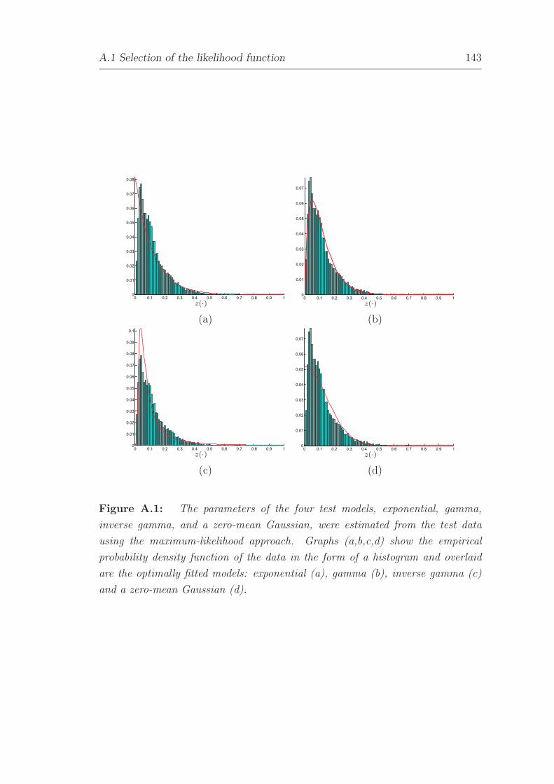
A.1 Selection of the likelihood function 143

0 0.1 0.2 0.3 0.4 0.5 0.6 0.7 0.8 0.9 10

0.01

0.02

0.03

0.04

0.05

0.06

0.07

0.08

z(·) z(·)

(a) (b)

0 0.1 0.2 0.3 0.4 0.5 0.6 0.7 0.8 0.9 10

0.01

0.02

0.03

0.04

0.05

0.06

0.07

0.08

0.09

0.1

z(·) z(·)

(c) (d)

Figure A.1: The parameters of the four test models, exponential, gamma,

inverse gamma, and a zero-mean Gaussian, were estimated from the test data

using the maximum-likelihood approach. Graphs (a,b,c,d) show the empirical

probability density function of the data in the form of a histogram and overlaid

are the optimally fitted models: exponential (a), gamma (b), inverse gamma (c)

and a zero-mean Gaussian (d).

144 Appendix

IVIIII II

2

4

6

8

10

12

14

16

1E3∆

i

model number, iIVIIII II

0

0.1

0.2

0.3

0.4

0.5

0.6

0.7

0.8

0.9

1

wA

IC

i

model number, i

(a) (b)

Figure A.2: The values ∆i in (a) indicate that the optimal choice in terms of

AIC criterion is the gamma distribution. This is further confirmed by the AIC

weights in (b), where it can be seen that there is nearly a 100% chance that the

gamma pdf explains the underlying data best among the four test models.

Based on the results form Figures A.1 and Figures A.2 the Gamma pdf was

chosen to model the distribution of the presence-measure values.

f(z; α, β) =1

βαΓ(α)xα−1e

− x

β , (A.3)

where a in b the ML estimates

α = 1.769, β = 0.066,

with 95% confidence intervals

p(1.719 < α < 1.818) = 0.95

and

p(0.064 < β < 0.068) = 0.95.

Appendix B

Discretization of continuous-time

models

The Bayesian probabilistic tracking scheme described in Section 2.5.5 is used to

combine the information from the visual model and the target’s dynamics in order

to arrive at better estimates of the target state (e.g., position). The dynamics of

target are modelled by continuous processes. However, since the data, i.e., images,

arrive at discrete time-steps, the continuous-time models have to be sampled at

those time-steps so that we can use them in the Bayesian estimation. Following

[151, 26] we provide here a derivation of the sampling process – the discretization.

We first give a general derivation of the discretization. These solutions have been

applied in Section 5.1 to yield a discretized counterpart of the continuous liberal

dynamic model (5.9). In this thesis we also refer to two dynamic models, which

are widely used in practice: the random-walk model and the nearly-constant-

velocity dynamic model. For completion, we derive these in Appendix B.1 and

Appendix B.2, respectively.

Let x(t) be a d-dimensional column vector describing the system state at time

t and let the system dynamics be described by the following linear relation

x(t) = Fx(t) + Gu(t) + Lw(t), (B.1)

where F is a d× d system matrix relating x(t) to its derivative x(t), G is a d× r

matrix that relates an r-dimensional vector, the control input u(t), to x(t), L

is a d-dimensional vector and where w(t) is a white-noise forcing function. Now

consider sampling this process at discrete times t0, t1, . . . , tk, . . . , such that the

difference between each pair of consecutive times is ∆t = tk+1 − tk. Assuming

piece-wise constant inputs, it can be shown that the solution to the differential

145

146 Appendix

equation (B.1) at time tk (see for example, [151] p. 84) is

x(tk) = Φ(∆t)x(tk−1) + Γu(tk−1) + W(tk−1) (B.2)

with

Φ(∆t) = eF∆t ∆= I + F∆t +

1

2!F2∆t2 +

1

3!F3∆t3 + . . . ,

Γ =

tk∫

tk−1

Φ(τ)Gu(τ)dτ ,

W(tk−1) =

tk∫

tk−1

Φ(τ)Lw(τ)dτ . (B.3)

where tk = tk−1 + ∆t, W(tk−1) is the driven response at tk due to the presence

of the white-noise input during the (tk−1, tk) interval, and is itself a white-noise

sequence. From now on, we will abbreviate notations of values at times tk by the

subscripts (·)k. Thus (B.2) may be written as

xk = Φ(∆t)xk−1 + Γuk−1 + Wk−1. (B.4)

To find the covariance matrix Qk−1 of the white-noise sequence Wk−1, we

have to evaluate the following expectation

Qk−1 = 〈Wk−1WTk−1〉

= 〈[tk

∫

tk−1

Φ(ξ)Lw(ξ)dξ][

tk∫

tk−1

Φ(η)Lw(η)dη]T 〉

=

tk∫

tk−1

tk∫

tk−1

Φ(ξ)L〈w(ξ)wT (η)〉LTΦ(η)T dξdη. (B.5)

Since the continuous input disturbance w(t) is assumed a white-noise random

process with a zero mean and a spectral density matrix Qc, we have

〈w(ξ)wT (η)〉 = Qcδ(ξ − η), (B.6)

where δ(ξ − η) is the Dirac-delta function. Finally, using (B.6), and assuming a

time-invariant system, we can rewrite (B.5) into

Qk−1 =

∆t∫

0

Φ(ξ)LQcLTΦ(ξ)T dξ. (B.7)

B.1 Random-walk dynamic model 147

The above equations describe the discretization process which we will now apply

to derive the random-walk and the nearly-constant-velocity model.

B.1 Random-walk dynamic model

The random-walk model assumes that changes in position arise purely due to a

random factor. In other words, the system velocity is modelled by a white-noise

sequence, i.e., x(t) = w(t). Thus dynamics of a one-dimensional system governed

by the random-walk is described by the following continuous-time stochastic

differential equation (s.d.e)

x(t) =

[

0 0

0 0

]

x(t) +

[

1

0

]

w(t), (B.8)

where the system state x(t) is composed of position and velocity

x(t) = [x(t), v(t)]T , and w(t) is a one-dimensional continuous white-noise

sequence with spectral density qc. Following (B.1-B.7) the discretized s.d.e. is

xk = Φxk−1 + Wk−1 (B.9)

Φ =

[

1 0

0 1

]

,

where Wk−1 is a white noise sequence with covariance matrix (B.7)

Q = qc

[

∆t 0

0 0

]

, (B.10)

Note that in (B.9) we write Φ instead of Φ(∆t) for brevity and that we have

dropped the subscript (·)k−1 in (B.10) since the covariance matrix Q depends

only on ∆t, that is, the difference between the consecutive time-steps.

B.2 Nearly-constant-velocity dynamic model

The nearly-constant-velocity model assumes that while the changes in the position

arise due to a nonzero velocity, the changes in the velocity arise purely due to a

random factor. In other words, the system acceleration is modelled by a white-

noise sequence, i.e., v(t) = w(t). Thus dynamics of a one-dimensional system

148 Appendix

governed by the nearly-constant velocity is described by the following continuous-

time stochastic differential equation

x(t) =

[

0 1

0 0

]

x(t) +

[

0

1

]

w(t), (B.11)

where the system state x(t) is composed of position and velocity

x(t) = [x(t), v(t)]T and w(t) is a one-dimensional continuous white-noise sequence

with spectral density qc. Following (B.1-B.7) the discretized s.d.e. is

xk = Φxk−1 + Wk−1 (B.12)

Φ =

[

1 ∆t

0 1

]

,

where Wk−1 is a white noise sequence with covariance matrix (B.7)

Q = qc

[

13∆t3 1

2∆t2

12∆t2 ∆t

]

, (B.13)

It is interesting to see that the covariance matrix Q implies correlation between

current perturbation Wk−1 in position and velocity, even though w(t) in (B.13)

is a one-dimensional white-noise process acting only on the target velocity at the

time instant t, and is thus not correlated with any other time instant. Note that

the correlation in the discretized form (B.13) arises because we are integrating the

effects of the white-noise process over a nonzero interval ∆t between consecutive

time-steps.

Biography

Matej Kristan was born on October 30th, 1978 in Ljubljana. He finished a

four-year secondary school programme at gimnazija Ledina and enrolled in the

Faculty of Electrical Engineering, University of Ljubljana in 1997. Between

years 2000 and 2003 he worked as a student with the Laboratory of Modelling,

Simulation and Control on a robot-soccer project. The focus of his work was

camera calibration and tracking. From year 2001 to 2002 he was employed by

Zamisel d.o.o. where he worked as a development engineer on several projects.

Results of his work were methods for automatic online adjustment of camera

parameters, methods for rapid merging of 3D triangulated objects and automatic

methods for calibration of laser CNC machines. In 2003 he received a diploma

degree from the Faculty of Electrical Engineering, University of Ljubljana in the

field of automatics – cybernetics. His thesis was on a system for tracking in

robot soccer. In 2003 he also started his postgraduate study at the same faculty

and joined the Laboratory of Imaging Technologies, where he worked from 2003

to 2005 on a commercial project of tracking in sports. In 2005 he received a

master’s degree with thesis on application of sequential Monte Carlo methods to

tracking in computer vision, and enrolled in a doctoral programme at Faculty of

Electrical Engineering, University of Ljubljana. In 2006 he was employed as a

researcher at the Visual Cognitive Systems Laboratory, Faculty of Computer and

Information Science, University of Ljubljana. In 2007 he was also employed as a

researcher at Machine Vision Group of prof. dr. Stanislav Kovacic at the Faculty

of Electrical Engineering, University of Ljubljana. Between years 2004 and 2008

he attended various international winter and summer schools on computer vision

and statistical pattern recognition. Currently he is a researcher at the Visual

Cognitive Systems Laboratory and the Machine Vision Group. Between years

2003 and 2008 he authored or coauthored six scientific journal papers, twenty

conference papers, a technical report, a book chapter, a diploma thesis and a

master’s thesis.

149

150 Biography

Personal data

First and last name Matej Kristan

Date of birth October 30, 1978

Birthplace Ljubljana

Home address Rozna Dolina c.VIII/29a, Ljubljana

Citizenship Slovenian

Education

1997 Finished a Secondary School gimnazija Ledina.

1997 - 2003 Study in a five-year university programme at University of

Ljubljana, Faculty of Electrical Engineering.

September, 2003 Graduated at Faculty of Electrical Engineering, University of

Ljubljana, Slovenia. Title of the thesis: Sledenje objektov v

robotskem nogometu.

2003 - 2005 Postgraduate student, Faculty of electrical engineering,

University of Ljubljana, Slovenia.

May, 17-20, 2004 Advanced School on Computer Vision, Pattern Recognition

and Image Processing, Verona, Italy. Invited speaker:

Prof. Brendan J. Frey, Course title: Bayesian Networks

and Algorithms for Inference and Learning: Applications in

Computer Vision, Audio Processing, and Molecular Biology.

September, 2005 Reached a Master-of-Philosophy degree, Faculty of electrical

engineering, University of Ljubljana, Slovenia. Title of the

thesis: Sekvencne Monte Carlo metode za sledenje oseb v

racunalniskem vidu.

2005 - 2008 Doctoral study at Faculty for Electrical Engineering,

University of Ljubljana.

August, 25-29, 2007 DIRAC/COSY Summer Workshop on Multi-Sensory

Modalities in Cognitive Science, Gerzensee, Switzerland.

March, 9-14, 2008 VISIONTRAIN Thematic school on Understanding Behavior

from Video Sequences, Les Houches, France.

Biography 151

Professional and academic experience

2000 - 2003 Laboratory of Modelling, Simulation and Control,

Faculty of Electrical Engineering, University of Ljubljana,

Slovenia. Position: Student, Work: Spare-time work on a

multi-agent management system in robot soccer. Areas of

focus: tracking and camera calibration.

2001 - 2002 Zamisel d.o.o, Ljubljana, Slovenija. Position: Development

engineer, Work: Development of methods for automatic

calibration of laser CNC machines. Methods for rapid

merging of triangulated 3D objects. Automatic procedures

for camera parameters optimization for visual inspection.

2003 - 2005 Laboratory of imaging technologies, Faculty of Electrical

Engineering, University of Ljubljana, Slovenia. Position:

Researcher, Work: Development of a commercial application

for motion analysis in team sports. Commissioned by:

Inspireworks, NY, USA.

2005 - 2006 Laboratory of imaging technologies, Faculty of Electrical

Engineering, University of Ljubljana, Slovenia. Position:

Researcher, Work: Development of laser system for measuring

dimensions of facade plates. Commissioned by: Trimo d.o.o,

Ljubljana.

2006 - 2008 Visual Cognitive Systems Laboratory, Faculty of

computer and information science, University of Ljubljana,

Slovenia. Position: Researcher, Work: Development of

cognitive systems for cognitive assistant, (EU project CoSy).

2006 - 2007 Laboratory of imaging technologies, Faculty of Electrical

Engineering, University of Ljubljana, Slovenia. Position:

Researcher, Work: M2-0156 project CIVaBIS, sponsored by

Ministry of Defence of Republic of Slovenia.

152 Biography

2007 - 2008 Laboratory of imaging technologies, Faculty of Electrical

Engineering, University of Ljubljana, Slovenia. Position:

Researcher, Work: technological project MIR, ”Autonomous

vessel for measurement and logistics” – APSIS, sponsored by

Ministry of Defence of Republic of Slovenia.

2007 - 2008 Laboratory of imaging technologies, Faculty of Electrical

Engineering, University of Ljubljana, Slovenia. Position:

Researcher, Work: M3-0233 project PDR, sponsored by

Ministry of Defence of Republic of Slovenia.

Honors and awards

2005 Received a best student paper award at International

Symposium on Image and Signal Processing and Analysis

ISPA 2005.

Published work

1.01 Original Scientific Article

[1] M. Kristan, M. Perse, S. Kovacic, and J. Pers, Closed-world tracking of

multiple interacting targets for indoor-sports applications, Computer Vision

and Image Understanding (2008), in press.

[2] M. Perse, M. Kristan, G. Vuckovic, S. Kovacic, and J. Pers, A trajectory-based

analysis of coordinated team activity in a basketball game, Computer Vision

and Image Understanding (2008), in press.

[3] M. Kristan, M. Perse, S. Kovacic, and J. Pers, Sledenje vec igralcev v sportnih

igrah na podlagi vizualne informacije, Electrotechnical Review 74 (2007),

no. 1-2, 19–24.

[4] M. Kristan, J. Pers, M. Perse, and S. Kovacic, A Bayes-spectral-entropy-

based measure of camera focus using a discrete cosine transform, Pattern

Recognition Letters 27 (2006), no. 13, 1419–1580.

[5] G. Klancar, M. Kristan, and R. Karba, Wide-angle camera distortions and

non-uniform illumination in mobile robot tracking, Robotics and Autonomous

Systems 46 (2004), no. 2, 125 – 133.

[6] G. Klancar, M. Kristan, and S. Kovacic, Robust and efficient vision system

for group of cooperating mobile robots with application to soccer robots, ISA

Transactions 43 (2004), no. 3, 329–342.

1.08 Published Conference Papers

[7] V. Sulic, J. Pers, M. Kristan, A. Jarc, M. Perse, and S. Kovacic, Izvedba

algoritma racunalniskega vida na omrezni kameri, Racunalniska obdelava slik

in njena uporaba v Sloveniji (P. Bozidar, ed.), 2008, pp. 35–40.

153

154 Published work

[8] M. Kristan, D. Skocaj, and A. Leonardis, Incremental learning with Gaussian

mixture models, Computer Vision Winter Workshop, 2008, pp. 25–32.

[9] M. Perse, M. Kristan, J. Pers, G. Vuckovic, and S. Kovacic, Temporal

segmentation of group motion using Gaussian mixture models, Computer

Vision Winter Workshop, 2008, pp. 47–54.

[10] D. Skocaj, M. Kristan, and A. Leonardis, Continuous learning of simple

visual concepts using Incremental Kernel Density Estimation, International

Conference on Computer Vision Theory and Applications, 2008, pp. 598–604.

[11] M. Kristan, J. Pers, A. Leonardis, and S. Kovacic, A hierarchical dynamic

model for tracking in sports, Proceedings of the sixteen Electrotechnical and

Computer Science Conference, ERK07, September 2007, pp. 187–190.

[12] D. Skocaj, A. Vrecko, M. Kristan, B. Ridge, G. Berginc, and A. Leonardis,

Interaktiven sistem za kontinuirano ucenje vizualnih konceptov, Proceedings

of the sixteen Electrotechnical and Computer Science Conference, ERK07,

2007, pp. 167–170.

[13] M. Perse, M. Kristan,J. Pers, S. Kovacic, Automatic evaluation of organized

basketball activity, Computer Vision Winter Workshop 2007 (Helmut Grabner

Michael Grabner, ed.), 2007, pp. 11–18.

[14] J. Pers, M. Kristan, M. Kolbe, and S. Kovacic, Tailgating detection

using histograms of optical flow,Computer Vision Winter Workshop 2007

(Helmut Grabner Michael Grabner, ed.), 2007, pp. 19–26.

[15] M. Kristan, J. Pers, A. Leonardis, and S. Kovacic, Probabilistic tracking using

optical flow to resolve color ambiguities, Computer Vision Winter Workshop

2007 (Helmut Grabner Michael Grabner, ed.), 2007, pp. 3–10.

[16] F. Erculj, G. Vuckovic, J. Pers, M. Perse, and M. Kristan, Razlike v opravljeni

poti in povprecni hitrosti gibanja med razlicnimi tipi kosarkarjev, Zbornik

naucnih i strucnih radova (N. Smajlovic, ed.), 2007, pp. 175–179.

[17] M. Kristan, J. Pers, M. Perse, and S. Kovacic, Towards fast and efficient

methods for tracking players in sports, Proceedings of the ECCV Workshop

on Computer Vision Based Analysis in Sport Environments (J. Pers and D. R.

Magee, eds.), May 2006, pp. 14–25.

Published work 155

[18] M. Perse, M. Kristan, J. Pers, and S. Kovacic, A template-based multi-player

action recognition of the basketball game, Proceedings of the ECCV Workshop

on Computer Vision Based Analysis in Sport Environments (J. Pers and D. R.

Magee, eds.), May 2006, pp. 71–82.

[19] J. Pers, M. Kristan, M. Perse, M. Bon, G. Vuckovic, and S. Kovacic, Analiza

gibanja igralcev med tekmami, Racunalniska obdelava slik in njena uporaba v

Sloveniji (P. Bozidar, ed.), 2006, pp. 97–103.

[20] M. Kristan, J. Pers, M. Perse, M. Bon, and S. Kovacic, Multiple interacting

targets tracking with application to team sports, International Symposium on

Image and Signal Processing and Analysis, September 2005, pp. 322–327.

[21] M. Perse, J. Pers, M. Kristan, G. Vuckovic, and S. Kovacic, Physics-

based modelling of human motion using kalman filter and collision avoidance

algorithm, International Symposium on Image and Signal Processing and

Analysis, September 2005, pp. 328–333.

[22] M. Kristan, J. Pers, M. Perse, and S. Kovacic, Bayes spectral entropy-based

measure of camera focus, Computer Vision Winter Workshop, February 2005,

pp. 155–164.

[23] M. Kristan, J. Pers, M. Perse, and S. Kovacic, Implementacija

Condensation algoritma v domeni zaprtega sveta,Proceedings of the thirteenth

Electrotechnical and Computer Science Conference, vol. B, September 2004,

pp. 179–182.

[24] M. Kristan and F. Pernus, Entropy based measure of camera focus,

Proceedings of the thirteenth Electrotechnical and Computer Science

Conference, vol. B, September 2004, pp. 179–182.

[25] J. Pers, M. Kristan, M. Perse, and S. Kovacic, Observing human motion

using far-infrared (FLIR) camera – some preliminary studies, Proceedings

of the thirteenth Electrotechnical and Computer Science Conference, vol. B,

September 2004, pp. 187–190.

[26] M. Perse, J. Pers, M. Kristan, and S. Kovacic, Vrednotenje ucinkovitosti

kalmanovega filtra pri sledenju ljudi, Proceedings of the thirteenth

Electrotechnical and Computer Science Conference, vol. B, September 2004,

pp. 191–194.

156 Published work

Technical reports

[27] M. Kristan, D. Skocaj, and A. Leonardis, Approximating distributions

through mixtures of Gaussians, LUVSS-TR-04/07, Faculty of Computer and

Information Science, University of Ljubljana, September 2007.

Monographs and Other Completed Works

2.01 Scientific Monographs

[28] G. Klancar, M. Lepetic, M. Kristan, and R. Karba., Mobile robots : New

research, ch. Vision System Design for Mobile Robot Tracking, pp. 117–141,

Nova Science Publishers, 2006.

2.09 Masters Thesis

[29] M. Kristan, Sekvencne Monte Carlo metode za sledenje oseb v racunalniskem

vidu, Masters thesis, Faculty of Electrical Engineering, University of

Ljubljana, September 2005.

2.11 Diploma Thesis

[30] M. Kristan, Sledenje objektov v robotskem nogometu, Diploma thesis, Faculty

of Electrical Engineering, University of Ljubljana, September 2003.

Izjava

Izjavljam, da sem doktorsko nalogo izdelal samostojno pod vodstvom mentorja

prof. dr. Stanislava Kovacica in somentorja prof. dr. Alesa Leonardisa. Izkazano

pomoc drugih sodelavcev sem v celoti navedel v zahvali.

V Ljubljani, 16. maj 2008.

mag. Matej Kristan, univ. dipl. inz. el.

157