SLAC-PUB-815 April 1971 U’H) and WP)

INELASTIC ELECTRON-PROTON SCATTERING

AT LARGE MOMENTUM TRANSFERS

G. Miller, E. D. Bloom, G. Buschhorn,* D. H. Coward, H. DeStaebler, J. Drees, ** C. L. Jordan, L. W. MO, *** R. E, Taylor

Stanford Linear Accelerator Center t Stanford University, Stanford, California 94305

J. I. Friedman, G. C. Hartmann, ‘ft H. W. Kendall, R. Verdier Physics Department and Laboratory for Nuclear Sciencettt

Massachusetts Institute of Technology, Cambridge, Massachusetts 02139

ABSTRACT

Differential cross sections for electrons scattered inelastically

from hydrogen were measured at 18’, 26’, and 34’. The range of

incident energy was 4.5 to 18 GeV, and the range of four momentum

transfer squared was 1.5 to 21 (GeV/c)2. With the use of these data

in conjunction with previously measured data at 6’ and loo, the con-

tributions from the longitudinal and transverse components of the

exchanged photon have been separately determined. The values of

the ratio of the photoabsorption cross sections aS/uT were in the

range 0 to 0.5.

(Submitted to Phys. Rev. Letters .)

* Present address: DESY, Hamburg, Germany.

** Present address: Bonn University, Bonn, Germany..

*** Present address: Department of Physics and the Enrico Fermi Institute, University of Chicago, Chicago, Illinois.

t Work supported by the U. S. Atomic Energy Commission. tt Present address: Xerox Corporation, Rochester, New York.

ttt Work supported in part by the U. S. Atomic Energy Commission under Contract No. AT(30-1)2098.

The measurements we report here extend our earlier study of inelastic

electron-proton scattering at forward angles’ to larger angles (Q) , higher four-

momentum transfer squared (q2), and higher electron energy loss (v) and allow

a separation of the two electromagnetic structure functions of the proton. This

paper presents the results of the separation; a discussion of the q2 behavior of

these functions and the implications of the measurements with regard to the

question of scaling will be given in a second communicatiom2 The differential

cross sections d 2 cT/dfidE’ for inelastic electron-proton scattering have been

measured at the Stanford Linear Accelerator Center by detecting the scattered

electron at laboratory angles of 18’, 26’ and 34’. Measurements were made

at incident energies between 4.5 GeV and 18 GeV and at scattered electron mo-

menta between the limit set by elastic scattering kinematics and 2 GeV/c,

1.75 GeV/c and 1,5 GeV/c respectively for the three angles. These measure-

ments have been combined with our earlier measurements at 6’ and 10’ to

provide a separation for various values of q2 in the range from 1.5 to 11.0 (GeV/c)2

over a range of W, from 2.0 to 4.0 GeV, where W is the mass of unobserved

hadronic state.

In making the separation we have found it convenient to use the representa-

tion for the differential cross section employing the absorption cross sections,

O-T and us, for virtual photons with transverse and longitudinal polarization

components respectively. 3 On the assumption of one-photon exchange, the dif-

ferential cross section in the laboratory frame can be written as follows’:

d2@,E,E’j d0dE ’ = TT (o,ts2,ws + EUS tq2,,3) (1)

1 E= l

1+2(l+.v2/q2) tan2 ; ) ’ O&E<1 0

-2-

The quantity K = (d - M;)/2Mp, where Mp is the rest mass of the proton,

v=E-E’, andq2 = 4EE ’ sin2 8/2, E is the incident electron energy, and E’ is

the scattered energy. The measurements were taken over a large region of

q2, IV2 space as shown in Fig. 1, in order to provide a sufficiently fine grid

of data so that the unfolding of radiative effects could be accomplished in a

model-insensitive way. Radiatively corrected cross sections at constant values

of q2 and w2 for different values of E (which corresponds to different values of

0) allow the separate determination of oT and os, which yields R, defined as

The following is a description of the experimental equipment and technique

used to extract these results, with emphasis placed onmodifications and problems

specific to this experiment. The incident electron beam was typically defined

in energy to AE/E = f 0,50/o, and was focussed to a spot approximately 3 mm

high and 6 mm wide. The incident beam position and angle, monitored con-

tinuously throughout the experiment, remained constant to f 1 mm and f 0,l

mrad, respectively. The number of incident electrons was measured to an

absolute accuracy of k 0,5% by two toroidal beam monitors which were inter-

calibrated with a Faraday cup several times during the experiment. Collima-

tion studies of the incident beam were made to eliminate the possibility of a low

energy, large area beam halo which could introduce systematic errors in the

data taken at low secondary momenta.,

The liquid hydrogen target was specially designed to handle the very large

beam intensities used in this experiment. These were as high as 50 mA, in a

1.6 psec beam pulse, at repetition rates up to 360 times per second. The con-

densing target contained a pump which recirculated the liquid hydrogen in a closed

loop from the target cell through a heat exchanger in contact with a liquid hydrogen

-3-

reservoir. Extensive tests showed that the recirculation eliminated variations

of target density with variations of electron beam cross-sectional area and in-

tensity, to an accuracy of 2% in the scattering cross section. In addition, the

density was shown to be constant within * 1% throughout the actual experiment by

detecting with the SLAC 1.6 GeV/c spectrometer protons recoiling elastically

from the target. The density of the liquid hydrogen was 0.070 g/cm3, deter -

mined from the temperature of the hydrogen measured by two hydrogen cryo-

meters inserted in the target above and below the beam line. The 7-cm diameter

target cell was an aluminum cylinder with .003 inch thick walls. The wall con-

tribution to the scattering was measured by using an identical, but empty, alu-

minum cylinder mounted directly below the target assembly. Scattering from

the replica target and other windows was typically 10% of the full target rate.

The scattered particles were momentum analyzed by the SLAC 8 GeV spec-

trometer . The spectrometer focuses point-to-point and disperses momentum

in the vertical plane, and focuses line-to-point and disperses the horizontal scat-

tering angle in the horizontal plane. The magnets were calibrated to the same

standard shunt as the magnets defining the incident beam energy. The alignments

of the magnetic elements were frequently monitored during the experiment. All

observed misalignments were such as change a ray by less than one-fifth of the

designed resolution. In order to calculate the acceptance of the spectrometer,

a model was derived that reproduced optics measurements obtained by directing

the incident beam into the spectrometer and mapping out the acceptance with a

large family of rays of various energies and angles. The momentum dispersion

was approximately 3 cm/%, and the horizontal projected angle dispersion was

approximately 4.5 cm/mrad. The vertical pro jetted angle acceptance,

-4-

approximately 60 mrad, was determined by lead masks located before the last

quadrupole magnet. The total acceptance of the spectrometer An(Ap/p) was

25.4 (mrad)2. This was calculated analytically and by a Monte Carlo method.

The calculations agreed to & 1%.

Particle detection, identification and angle-momentum measurements were

accomplished by a system of detectors consisting in sequence of a threshold gas

Cerenkov counter (C), a large plastic scintillation counter for triggering purposes,

a scintillation counter hodoscope of 55 horizontal elements, a scintillation counter

hodoscope of 41 vertical elements, another large trigger counter, a telescope of

three scintillation counters preceded by one radiation length of lead (DEX) , and

a total absorption, lead-lucite shower counter (TA) D

The two orthogonal hodoscopes defined the resolution of the spectrometer

to & 0.05% in momentum and jz 0.15 mrad in horizontal scattering angle, A

restricted set of these hodoscope counters was used to define a smaller accept-

ance to investigate possible effects due to scattering from lead that masked

the hodoscopes 0 Average cross sections calculated with the total acceptance and

with the restricted acceptance agreed to 1% in the case where the cross sections

were not strongly varying with momentum. The calculations of the acceptance

were considered accurate to f 2%.

An on-line computer system, utilizing an SDS 9300 computer, scanned the

hodoscope buffers after each event, the charge monitors and six analog-to-digital

converters. This information was written on magnetic tape for later analysis.

A continuously updated cross section as well as updated detector efficiencies

and inefficiencies due to hodoscope multiple tracks were evaluated on-line using

a fraction of the events written on tape. The largest instantaneous counting rates

occurred in the large trigger counters and were kept less than 5 per machine

-5-

pulse by regulating the incident beam intensity. The fast electronic dead times ‘

effects were less than 1%. The number of events per pulse was kept at rates

less than 0.3 events per pulse.

The electron yields and cross sections for a particular E, E’, 6 setting,

target type, and spectrometer polarity were calculated by counting the number of

events on the data tape satisfying three different requirements, allowing succes-

sively greater electron-pion discrimination. The discrimination requirements

were: (a) a large pulse height from the TA counter corresponding to a 99% effi-

ciency for a pure electron sample; (b) a signal from the Cerenkov counter plus

requirement (a) ; and (c) large pulse heights from all three DEX scintillation

counters plus condition (b) . Where the three cross sections agreed the least

restrictive requirement having the largest number of successful events was used.

All events were required to have good signals from both trigger scintillation

counters and to represent particles unambiguously passing through the restricted

set of hodoscope counters.

Discrimination of electrons from pions became a problem at the lowest

secondary energies 0 The largest pion to electron ratio encountered was 3OO:l

where the pion rejection of the combined system (C)(DEX)(TA) was about 2~10~~1,

and the electron efficiency was 0.72. This low efficiency was due to the DEX

system which had an energy dependent efficiency for electrons that ranged from

0 0 74 at 2 GeV to 0,88 at 8 GeV and had an uncertainty of f 1. 5%b. For most

points, DEX was not used, and the electron efficiency was 0.97. The error due

to pion contamination was I 2%.

Corrections were made for the electron detection efficiency of all counters,

for the computer logging deadtime (less than 15%) and for ambiguous hodoscope

bit patterns (typically 7%) D The final measured cross section was corrected by

subtracting the cross section for electrons scattered from the target walls and

-6-

the contribution from electrons coming from no decay and pair production,

which was measured by reversing the polarity of the spectrometer and was

negligible over most of the spectra except at the lowest scattered energies

where it was always less than 25Y7c0

The measured cross sections were corrected for radiative effects in the

following way, First, the elastic radiative tail was subtracted. This was cal-

culated using the formula of Tsai’ for electron bremsstrahlung during the elastic

scattering which is exact to lowest order in (Y D Radiative energy degradation of

the incident and final electrons by the surrounding target material was also in-

eluded along with corrections 7 for multiple photon effects and radiation from

the recoiling proton. After the subtraction of the elastic tail, the inelastic

radiative effects were removed in an unfolding procedure using a peaking-

factorization approximation which allowed the radiative tail to be expressed as

the sum of two one-dimensional integrals involving the previously corrected

cross sections at the same angle. The particular version of the peaking-

factorization approximation used was determined by a direct comparison with

an exact calculation of the inelastic radiative tail, assuming a model which

approximated the experimentally determined inelastic form factors D

The inelastic radiative tail corrections were assigned an error of -I 10% to

take into account both the inaccuracy of the peaking approximation and errors

introduced by interpolation of the cross section. The different methods of inter-

polation used changed the corrected cross sections by less than half of the sta-

tistical error 0 The elastic tail corrections were assigned an average error of

f 3% which reflect uncertainties as large as 570~ The maximum total radiative

correction was 300/o, and the corrections were generally smaller than those at

the lower angles. ’

-7-

Elastic e-p scattering was measured for nine combinations of incident en-

ergy and scattering angle, and two different analyses were done. First, the

effects of radiation were unfolded using a method described in another pub-

lication. 8 Secondly, the theoretical cross section was folded with radiation

effects, the incident energy spectrum, and the spectrometer resolution using

the elastic form factors previously reported by the MIT-SLAC collaboration’

together with the elastic scattering measurements taken at 6’ and 10’ with the

20 GeV spectrometer. Both methods gave similar results that indicated that

the apparatus had no systematic errors comparable to the statistical errors

of approximately 3%. This result is especially important for those

separations of o T and os that also rely on data taken at small angles with the

20 GeV spectrometer. Typically, a systematic 3% difference between the 6’

and 10’ data and the present data would change the ratio R = oS/oT by 0 D 06.

This uncertainty is small compared to the statistical errors in the values of R.

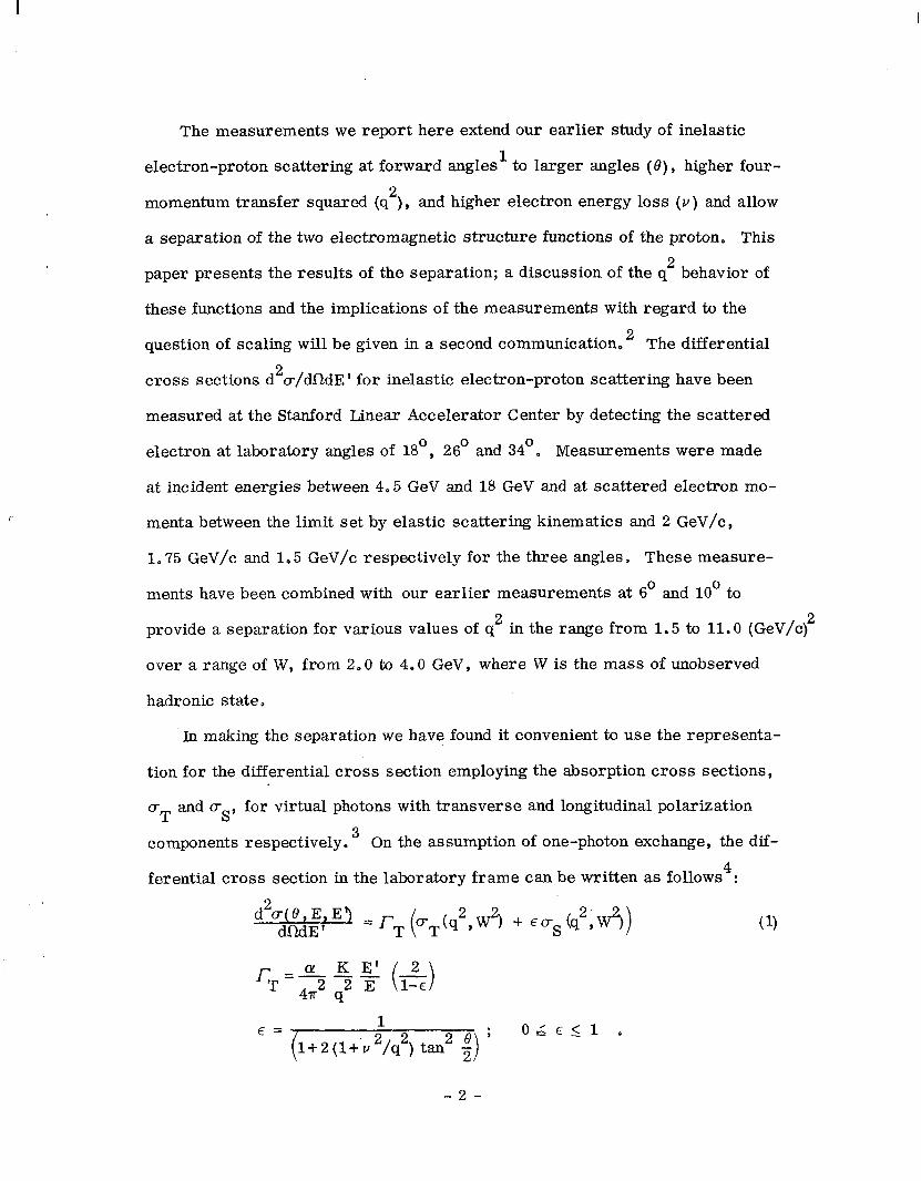
Figure 2 shows the radiatively corrected spectrum for E = 18 GeV, and

0 =26’ along with the radiative correction factor, defined as the ratio of the

final corrected cross section to the measured cross section.

Table I gives the values of the radiatively corrected cross sections for

which W 1 1,8 GeV. The quoted errors reflect both counting statistics and

parts of other estimated uncertainties two of which are the errors described

above for the elastic and inelastic radiative tails. Not included is an additional

overall systematic error that is estimated to be f 5%.

The shaded area of the q2 - w2 plane in Fig. 1 shows the kinematic range

over which us and oT can be separated, requiring data at a minimum of three

values of E D Actual data points at different angles for the same values of q2

and W2 exist only for q2 = 4(GeV/c) 2; W=2, 3, and 4 GeV, However, the data at

-8-

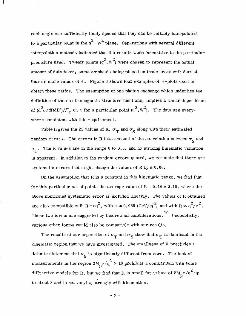
each angle are sufficiently finely spaced that they can be reliably interpolated

to a particular point in the q2, 2 plane, Separations with several different

interpolation methods indicated that the results were insensitive to the particular

procedure used, Twenty points (q2, W2) were chosen to represent the actual

amount of data taken, some emphasis being placed on those areas with data at

four or more values of e D Figure 3 shows four examples of ~-plots used to

obtain these ratios. The assumption of one photon exchange which underlies the

definition of the electromagnetic structure functions, implies a linear dependence

of (d20/dfldE ‘),‘rT on 6 for a particular point (q2, W2). The data are every-

where consistent with this requirement.

Table11 gives the 23 values of R, oT and os along with their estimated

random errors. The errors in R take account of the correlation between crs and

aTO The R values are in the range 0 to 0,5, and no striking kinematic variation

is apparent. In addition to the random errors quoted, we estimate that there are

systematic errors that might change the values of R by f 0.06.

On the assumption that R is a constant in this kinematic range, we find that

for this particular set of points the average value of R = 0.18 f 0.10, where the

above mentioned systematic error is included linearly. The values of R obtained

are also compatible with R = aq2, with a z 0.035 (GeV/cr2, and with R 2 q2/v2Q

These two forms are suggested by theoretical considerations. 10 Undoubtedly,

various other forms would also be compatible with our results.

The results of our separation of uT and us show that uT is dominant in the

kinematic region that we have investigated. The smallness of R precludes a

definite statement that us is significantly different from zero. The lack of

measurements in the region 2Mpv/q2 > 10 prohibits a comparison with some

diffractive models for R, but we find that R is small for values of 2Mpv/q2 up

to about 8 and is not varying strongly with kinematics.

-9-

The group wishes to thank Professor W.K.H. Panofsky, the Spectrometer

Facilities Group,and the Technical Division under R. B. Neal for their support

in this project.

REFERENCES

1. E. D. Bloom et al,, Phys. Rev. Letters 23, 930 (1969) .,

2. Submitted for publication in Phys. Rev. Letters,

3. L. Hand, Ph.D. dissertation, Stanford University (1961) and Phys. Rev.

129, 1834 (1963).

4, The differential cross section can be expressed in terms of two structure

functions WI and W2 such that

d20 28 dndE’=

32 402(E

‘I4 cos 2 ; + 2W1(q2, W2) sin 5 1

These structure functions are related to the two absorption cross sections

for virtual photons in the following way

wl=-+- u 4ncY T

A detailed discussion of these quantities is given, for example, by

F. Gilman, Phys. Rev. 167, 1365 (1968),

5. R. E. Taylor, International Symposium on Electron and Photon Interactions

at High Energies, Stanford Linear Accelerator Center (1967) .,

6. L. W. MO and Y. S. Tsai, Rev. Mod Phys. 4J, 205 (1969).

7. Guthrie Miller, Ph.D. dissertation, Stanford University (1970)) Report No.

SLAC-129. The appendix contains the exact statement of the formulas used

to radiatively correct these data. Multiple photon corrections are different

from Ref. 6.

8. P. N. Kirk et al., to be submitted to Phys . Rev. --

- 10 -

I

9. D. H. Coward et al., Phys. Rev. Letters 3, 292 (1969).

10. The kinematic dependence R = aq2, where a is a constant, is compatible

with the gauge invariance requirement that us = 0 at q2=0. The relation

R =q2/v 2 would hold if, in the laboratory frame,

where p is the initial proton state, A is an arbitrary final state, j; and jy

are the longitudinal and transverse current operators respectively, and the

sum is over all possible final states. Such behavior leads to the relation

between the structure functions, Wl and W2, uW2 = (q2/v)Wl.

TABLE CAPTIONS

I. Radiatively corrected differential cross sections for inelastic electron-

proton scattering. All measured points with W 2 1.8 GeV are listed. The

errors are approximately statistical standard deviations. An estimated

overall systematic error of f 50/c is not included.

II. R,uT,os,W1 and W2for23valuesof q2and W2usingdatatakenat 6’, loo, 18’,

26’ , and 34’. The errors arise from the propagation of the errors given

in Table I. The effects of overall systematic errors are not included. We

estimate that systematic errors could make R uncertain by about f .06.

- 11 -

I

TABLE I

Radiatively Corrected Cross Sections for W > 1.6 GeV

0 de@ -

26

E' Gev) G 1.750

1.500

I.250

I. 000

!.?50

!.500

!.250

1.000

L.750

L.600

1.400

1.200

1.020

1.750

L.500 L.250

2.500

2.250

2.000

1.750

1.460

1.250 3.ooo 2.750

2.500

2.250

2.000

1.75c

1.5oc L.250

GG

3.000

2.750

2.500

2.250

2.000

1.750

1.500 1.250

3.250

3.ooc

2.75c

2.5oc

2.25(

2.00(

1.7%

1.50(

e deg) z

26

E

(G-N

d20/dFLdE' 10 -35

Cll12/S.PGeV)

E

1-v)

d2a/dfldE' [1o-35 cm'/sr-GeV)

12.9 * 1.2 15.3 l 1.7 21.5 l 1.7 25.7 t 2.5

32.9 * 4.1

39.4 f 5.2

45.7 l 7.3

56. f 10.

E

'Gev)

E'

GeV)

d20/dfldE' .0-35 cm2/sr-GeV)

1600. l 430,

1000. * 450.

1079. l 54.

!413. l 75.

$593. l 93.

2510. l 120.

460. * 15.

572. * 17.

779. * 44.

957. + 36.

L036. f 50.

1229. zt 65.

6.700 !.940 1.750

t.500

i.250

3.000

1.750

s.750

3.500

3.250

3.000

2.750

2.500

2.270

2.000

1.750 4.500

4.250

4.000

3.750

3.500

3.250

3.000

2.750

2.500

2.250

2.000

1.670 5.000

4.750

1.500

L.250

4.000

3.750

3.500

3.250

3.000

2.750

2.500

2.250

2.000

1.750 5.500

5.250

5.000

4.750

4.500

4.250

4.000

LE.030

4.501

4.501 1.250

!.OOO

212.6 t 7.6

263.1 ilO. 340. l 14.

407. + 19. 504. t25.

585. f 51.

32.2 f 2.0

57.2 + 3.0

91.7 t 3.7

119.9 * 5.0 154.9 f 6.0 195.5 + 9.7 229, f 12. 275. f 17. 317. * 20.

4.70 i .40

9.34 f .99

17.7 f 1.0 25.9 + 1.6

35.1 f 2.2

47.0 f 4.5

63.4 f 6.2

76.9 * 7.7

91.2 t 9.9 113. * 12. 121. f 17. 161. + 23.

6.503 I.500

I. 000

!.500

3.000

1.760

4.500

4.000

3.500

3.000

2.500

2.000

8.696

I.905

15.006

L8.030

0.598

81. t 16.

404. * 22. 34

533. l 31.

652. l 41.

5.795 108.0 f 7.6 175.3' I 9.6 252. l 21.

356. t 33.

24.6 * 1.6

36.2 f 3.3

62.4 t 5.1

90.4 * 0.0

125. l 12.

153. f 21.

3.02t .35

8.6Oi .57

15.03i .66

26.1 l 1.2

36.4 t 2.9

47.2 f 4.4

10.3 * 1.4

104. * 13.

1330. + 130.

160.6 + 6.3 LO.404

13.299

5.500 Fl. 000 4.500

3.940

3.500

3.000

2.500

2.000

7.000

6.500

6.000

5.500

5.000

4.500

4.000

3.500

3.090

2.500

2.000

264. * 10. 409. + 16. 512. + 23.

604. + 32.

630. t 40.

751. * 47.

601. * 99. 19.68 t .so 49.2 l 1.9 93.0 f 3.6

135.6 t 5.6

178.2 t 7.7

206. f 15.

263. + 21.

306. * 28.

315. t 23.

417. * 49.

533. l 74.

7.08 + .35

15.17 l .56

29.9 * 1.1 44.6 t 1.7 64.3 i 2.6

06.9 t 3.4

101.1 * 7.4 122.8 * 9.4 145. l 12. 173. i 16. 191. * 20.

239. l 31.

271. * 54.

7.099

9.999

1.34 f .l? 2.07 i .26

5.55 * .39

8.07 t .50

13.63 * .Sl 16.4 * 1.5 23.3 + 1.3

31.6 t 1.8 39.6 + 2.3

45.9 * 4.3

52.0 i 5.4

62.7 f 7.6

76. * 10.

12.500 1.22* .19 3.52a .40

7.57a .55

10.32i .64

17.1 l 1.7

21.9 t 2.4 32.1 f 4.0 47.6 * 6.6

17.000

4.494

3.000

7.500

7.000

6.500

6.000

5.500

5.000

4.500

4.000

3.500

3.000

2.500

2.000

2.000

1.600

61. * 13. 0.85 f .25 14.996 2.29 * .36

4.30* .53

7.21* .99

11.6 * 1.8 16.7 t 2.0 19.6 t 3.0 32.6 t 5.4

79. t 15. .500 * .090

1.09 * .15 1.31 l .20 2.76 f .29

4.78 f .39

7.66 l .55

10.14 l .99

1410. l G?.

1516. f 81.

1.5

1.5

1.5

1.5

3.0

3.0

3.0

3.0

4.0

4.0

4.0

5.0

5.0

5.0

5.0

8.0

8.0

8.0

8.0

8.0

11.0

11.0

11.0

W

GeV

2.0

2.5

3.0

3.3

2.0

2.5

3.0

3.4

2.0

3.0

4.0

2.0

2.5

3.0

3.4

2.0

2.5

3.0

3.5

4.0

2.0

2.5

3.0

uT

lo-3o ml2

42.8 * 5.3

31.7 13.3

26.7 * 2.8

25.3 * 2.8

16.1 tt 1.9

15.8 =+z 1.5

15.7 * 1.6

13.3 3 2.0

8.8 -I 1.3

11.0 It 1.2

9.0 h 1.7

5.82zk .63

7.38% .57

8.23 -I .65

8.0 h 1.2

I..82 zk .25

2.95 k .27

3.55* .33

4.15rt .54

4.995 .74

.74* .16

1.44rt .18

1.82 rt .22

TABLEII

53

lo-3o m-n2

-2.8 z!z 6.6

4.8 -13.7

5.4 *I.3

5.8 zk3.6

. 75 & 2.6

2.0 zt2.0

1.7 zk2.2

4.3 xt2.8

2.0 hl.7

2.0 * 1.8

4.5 k3.0

1.0 z!c .9

1.1 ck .8

1.4 -Il.0

2.2 iz 1.8

.58zk .35

.57ic .41

1.30* .59

1.6 i 1.1

.3 ht.8

.34zk .23

.28zk .28

. 89zk .41

R

-.06 * .15

. 15 6 .13

.20* .14

.23zt .17

. 05 * .17

. 12 h .14

.11* .15

.32 ZIG .26

.23 h .23

. 18 rt .18

.5ozk .43

.17 * .17

. 15 * .12

.17 * .13

.27zk .27

.32 zk .24

.2Ozk .16

.37 4 .20

.39* .30

. 06 h .37

.46zt .40

.20* .22

.49 * .29

2Mpw1

1.19 zt .15

1.52 zk .16

1.93 * .20

2.26 * .25

.45 * .05

.76 &.07

1.14 * .ll

1.27 zt .19

.244* .038

.799* .086

1.22 k .23

. 162 zk .018

.353* ,027

.596 zk .047

,763 zk .113

.051* .007

.141* .013

.257 i .024

.42Ozt .055

.67 k .lO

. 021h ,004

.069 zt .008

. 132 -I .016

vw2

.290 zt .012

.344 zk .005

.343 rJz .007

.347* .Oll

.179 zk .009

.265 9 .008

.314* .014

.349* .019

.131* .005

.284 z!z .016

.369zk .039

.092 rt .004

. 169 h .005

.240& .009

.289 rfi .019

,039 k .002

.087 k .004

.157 * .009

.224 zk .021

.235-1 .048

.020-I .OOl

. 048 & .003

.102 rt .008

FIGURE CAPTIONS

1. The regions of the kinematic q2 - W2 plane covered by the measurements

at 18’, 26’ and 34’. The shaded area represents the region where data at

3 or more angles exist. Previously measured 6’ and 10’ data were also

used in the separations.

2. (a) The radiatively corrected inelastic scattering spectrum d2cr/dadE’ for

EO=18 GeV, 8=26’. (b) The radiative correction applied to the data as a

function of E’, defined as the ratio of the final corrected cross section to

the measured cross section.

3. Typical examples illustrating the separate determination of us and cT.

The straight solid lines are best fits to Eq. (1). The dashed lines indicate

the one standard deviation values of the fits. The assumption of one-

photon exchange made in calculating us and oT implies that linear fits

should be satisfactory. For the two upper graphs measured data exist

at each angle. For the two lower graphs the data were interpolated.

Effects of overall systematic errors are not included.

25

20

15

IO

5

0 C

M;-

I I I I

l 18” A 26” O 34”

W$,+m-rr) 2

25

W2 (GeV2) 1853C5

Fig. 1

1000 - I t ’ 1 I I

t ++t

E = 18.029 GeV 8 =26O

++

++ 100 = +

4 +

+

IO r +t

t

ELAST.lC PEAK ENERGY

I I I I ( \,

0 I 2 3 4 5 ‘6.122

I I I 1.2 - l ’

I.1 - l ee l

l

1.0 - l

l

l

0.9 -

l l

l

0.8 - l

l

0.7 I I I I 0 I 2 3.4 5

E’ [GgV]

Fig. 2

- BEST FIT A 9=6O A 8= IO”

-----I W=3.GeV R=O.20+0.14

20 I

0 0.5 1.0 E

I5

IO

5

5

4

3

0 8= 18” m 8= 26” 0 8= 34”

L

/

/

/ / / ih=3 GeV / R = 0.37 2 0.20

q2= 4(GeV/cj2 W=3 GeV R=0.18t0.18

0 0.5 1.0 c 1687C3

Fig. 3