sl-model for paired comparisons

SL-Model for Paired Comparisons

By

Morné Rowan Sjölander

submitted in

fulfillment of the requirements

for the degree of

MSc

in the

Faculty of Science

at the

Nelson Mandela Metropolitan University

November 2006

Supervisor: Prof I.N. Litvine

2

Contents

0 Acknowledgements 6

1 Literature Review 7

2 Notation 13

3 The S and SS Distribution 13

4 Paired Comparisons S- and SS-Experisment 37

5 The SL-Model

5.1 The General SL-Model 47

5.2 The Binary SL-Model 48

5.3 The DDic01 Binary SL-Model 48

5.4 The DD01 Binary SL-Model 49

6 Results and Examples Illustrating Properties of the

SL-Model 50

6.1 Results of the Solution to the SL-Model

6.2 Examples illustrating further Properties of the SL-Model 55

3

7 Real Life Application

7.1 Data 71

7.2 Methodology 79

7.3 Real Life Application of the General SL-Model 80

7.4 Real Life Application of the Binary SL-Model 101

7.5 Real Life Application of the DDic01 Binary SL-Model 121

7.6 Real Life Application of the DD01 Binary SL-Model 141

7.7 Comparison to other models 161

7.7.1 General SL-Model vs Binary SL-Model 166

7.7.2 General SL-Model vs DDic01 Binary SL-Model 170

7.7.3 General SL-Model vs DD01 Binary SL-Model 174

7.7.4 General SL-Model vs Binomial Poisson Model (Bayesian Solution) 178

7.7.5 General SL-Model vs Binomial Poisson Model (Max. Like. Solution) 182

7.7.6 General SL-Model vs Bradley-Terry Model 186

7.7.7 General SL-Model vs Poisson Model 190

7.7.8 General SL-Model vs Approx. Algorithm of Bayesian Solution Poisson

Model 194

7.7.9 General SL-Model vs Row Sum Method 198

7.7.10 Binary SL-Model vs DDic01 Binary SL-Model 202

7.7.11 Binary SL-Model vs DD01 Binary SL-Model 206

7.7.12 Binary SL-Model vs Binomial Poisson Model (Bayesian Solution) 210

7.7.13 Binary SL-Model vs Binomial Poisson Model (Max. Like. Solution) 214

7.7.14 Binary SL-Model vs Bradley-Terry Model 218

7.7.15 Binary SL-Model vs Poisson Model 222

7.7.16 Binary SL-Model vs Approx. Algorithm of Bayesian Solution Poisson

Model 226

7.7.17 Binary SL-Model vs Row Sum Method 230

7.7.18 DDic01 Binary SL-Model vs DD01 Binary SL-Model 234

7.7.19 DDic01 Binary SL-Model vs Binomial Poisson Model (Bayesian

Solution) 238

4

7.7.20 DDic01 Binary SL-Model vs Binomial Poisson Model (Max. Like.

Solution) 242

7.7.21 DDic01 Binary SL-Model vs Bradley-Terry Model 246

7.7.22 DDic01 Binary SL-Model vs Poisson Model 250

7.7.23 DDic01 Binary SL-Model vs Approx. Algorithm of Bayesian Solution

Poisson Model 254

7.7.24 DDic01 Binary SL-Model vs Row Sum Method 258

7.7.25 DD01 Binary SL-Model vs Binomial Poisson Model (Bayesian Solution) 262

7.7.26 DD01 Binary SL-Model vs Binomial Poisson Model (Max. Like.

Solution) 266

7.7.27 DD01 Binary SL-Model vs Bradley-Terry Model 270

7.7.28 DD01 Binary SL-Model vs Poisson Model 274

7.7.29 DD01 Binary SL-Model vs Approx. Algorithm of Bayesian Solution

Poisson Model 278

7.7.30 DD01 Binary SL-Model vs Row Sum Method 282

7.7.31 Binomial Poisson Model (Bayesian Solution) vs Binomial Poisson Model

(Max. Like. Solution) 286

7.7.32 Binomial Poisson Model (Bayesian Solution) vs Bradley-Terry Model 290

7.7.33 Binomial Poisson Model (Bayesian Solution) vs Poisson Model 294

7.7.34 Binomial Poisson Model (Bayesian Solution) vs Approx. Algorithm of

Bayesian Solution Poisson Model 298

7.7.35 Binomial Poisson Model (Bayesian Solution) vs Row Sum Method 302

7.7.36 Binomial Poisson Model (Max. Like. Solution) vs Bradley-Terry Model 306

7.7.37 Binomial Poisson Model (Max. Like. Solution) vs Poisson Model 310

7.7.38 Binomial Poisson Model (Max. Like. Solution) vs Approx. Algorithm of

Bayesian Solution Poisson Model 314

7.7.39 Binomial Poisson Model (Max. Like. Solution) vs Row Sum Method 318

7.7.40 Bradley-Terry Model vs Poisson Model 322

7.7.41 Bradley-Terry Model vs Approx. Algorithm of Bayesian Solution Poisson

Model 326

7.7.42 Bradley-Terry Model vs Row Sum Method 330

5

7.7.43 Poisson Model vs Approx. Algorithm of Bayesian Solution Poisson

Model 324

7.7.44 Poisson Model vs Row Sum Method 338

7.7.45 Approx. Algorithm of Bayesian Solution Poisson Model vs Row Sum

Method 342

7.7.46 Summary 346

8 Conclusion 349

9 References 350

6

0 Acknowledgements

I would like to thank the following for their support, guidance and encouragement.

1. To my God, who has blessed me in so many aspects of my life, the most precious of all

being, that I can know Him as my Friend.

2. Prof. Litvine, for suggesting the topic of the study, for his encouraging words, his

support and motivation, and all his assistance.

3. To my family, for their unconditional love, encouragement, prayers and everything

they mean to me.

4. All my friends, also my friends from NMMU including students and lecturers, for

there friendships and encouragement.

7

1 Literature Review

The method of paired comparisons can be found all the way back to 1860, where Fechner

made the first publication in this method, using it for his psychometric investigations [4].

Thurstone formalised the method by providing a mathematical background to it [9-11]

and in 1927 the method’s birth took place with his psychometric publications, one being

“a law of comparative judgment” [12-14].

The law of comparative judgment is a set of equations relating the proportion of times

any stimulus k is judged greater on a given attribute than any other stimulus j to the

scales and discriminal dispersions of the two stimuli on the psychological continuum.

The set of equations is derived from the following postulates:

1. Each stimulus when presented to the observer (judge) gives rise to a discrimininal

process which has some value on the psychological continuum of interest.

2. Because of momentary fluctuations in the organism, a given stimulus does not always

excite the same discriminal process, but may excite one with a lower or higher value in

the continuum. If any stimulus is presented to an observer a large number of times, a

frequency distribution of discriminal processes associated with that stimulus will be

generated. It is postulated that the values of the discriminal process are such that the

frequency distribution is normal on the psychological continuum. Each stimulus thus has

associated with it a normal distribution of dicriminal processes.

3. The mean and standard deviation associated with a stimulus is taken as its scale value

and discriminal dispersion respectively [12, 2].

8

“The principals of the Thurstone-Mosteller model may be found in [8]:

1. There is a set of stimuli that can be located on a subjective continuum.

2. Each stimulus when presented to an individual gives rise to a sensation in the

individual.

3. The distribution of sensations from a particular stimulus for a population of individuals

is normal.

4. Stimuli are presented in pairs to an individual, thus giving rise to a sensation for each

stimulus. The individual compares these sensations and reports which is greater.

5. It is possible for these paired sensations to be correlated.

6. The task is to space the stimuli (the sensation means), except for a linear

transformation.”[7].

The method of paired comparisons is a generalization of the two-category case of the

method of constant stimuli. In the method of constant stimuli, each stimulus is compared

with a single standard, whilst in paired comparisons each stimulus (object) serves in turn

as a standard. Thus with n stimuli (objects) there are 2

)1n(n −pairs of objects [2].

Paired comparisons is seen as a technique used to rank objects (or stimuli) with respect to

a certain property which may not be seen as measurable in the usual sense or have a

formal definition but can only be judged subjectively e.g. ranking the attractiveness of

models, taste of wine, social preferences, colour comparisons, choice behavior etc. Paired

comparisons is thus widely used be psychometricians. People known as judges are

presented with pairs of objects, and for each pair of object they assign a preference or a

score which can say object 1 is better or worse than object 2, or object 1 is 3 times better

9

than object 2, or object 1 scores 5 while object 2 scores 6 etc. all depending on which

model of paired comparisons is used and the nature of the objects in the experiment. This

data is then inputted to the model, and then numbers known as weights are received for

each object. These numbers are then used to rank the objects i.e. the object with the

highest weight is ranked first, the object with the second highest weight is ranked second

etc. [4, 7].

The reason why objects are compared two at a time is because this avoids what is known

as sensory fatigue, which is the lack of concentration and the confusion believed to be

experienced by a person if he/she has to evaluate more than two objects at a time. Paired

comparisons is however also used in many other applications where objects are to be

compared in pairs for other reasons e.g. in sport statistics, the way lots of games work is

that teams or players play against each other two at a time, and then a score is obtained

from each game. Various other applications e.g. economic, military etc. of the method of

paired comparisons are also present [7].

Some of the main models for paired comparisons are the following:

Thurstone-Mosteller Model

Linear Model

Bradley-Terry Model

Regression Model

Poisson Model

Poisson Model (Approximate Algorithm of Bayesian Solution)

Binomial-Poisson Model (Bayesian Solution)

10

Binomial-Poisson Model (Maximum Likelihood Solution)

Row Sum Method and Generalised Row Sum Method

Analytical Hierarchy Process (AHP)

Haines-Litvine Model (Exponential AHP)

The last one and first four of the above models are continuous models for paired

comparisons; the next four are examples of discrete models, while the remaining two are

distribution-free models/method [7].

At first there were only continuous models for paired comparisons - discrete models are

quite new. Litvine and Hilliard-Lomas were the first to introduce models for discrete

populations in 1996 some being the poisson model, the poisson model (approximate

algorithm of bayesian solution), the binomial-poisson model (bayesian solution) and the

binomial-poisson model (maximum likelihood solution) [6, 7].

Before 1996, paired comparisons models for discrete distributions had not been

successfully constructed. Continuous models were used on discrete data, in which case

many assumptions that should have been met for using such models have been violated.

These violations were simply overlooked [5].

If score is discrete in nature, but is quite high generally then we can use continuous

models by approximating the score with continuous random variables. Examples of this

are in sports like rugby or basketball. However, if score is discrete and quite small like in

sports like soccer, tennis or hockey, using continuous approximations is not good.

In the models for paired comparisons, an underlying distribution of the scores is assumed,

except for the distribution-free models/methods in which no underlying distribution is

assumed. Obviously, a continuous model assumes a continuous underlying distribution

11

and a discrete model assumes a discrete underlying distribution hence the classification of

the model.

The Thurstone-Mosteller model assumes a normal distribution whilst the Bradley-Terry

model assumes quite a wide class of distributions, one of the most important being the

exponential distribution. The Haines-Litvine Model assumes an exponential underlying

distribution but utilizes ratios of underlying random variables [7].

The poisson model and the poisson model using an approximate algorithm of bayesian

solution assumes the underlying distribution of the scores is the Poisson distribution,

while the binomial-poisson model (bayesian solution) and the binomial-poisson model

(maximum likelihood solution) was developed in the sports context (football) as follows:

Xi|ni ~ Binomial(ni, pj)

Xj|nj ~ Binomial(nj, pi)

Where Xi and Xj are the number of goals scored in a match between team i and team j,

and ni and nj are the number of situations when the respective team had a real possibility

to score a goal and are distributed as follows:

ni ~ Poisson(λi)

nj ~ Poisson(λj)

It can be shown that:

Xi ~ Poisson(λipj)

Xj ~ Poisson(λjpi)

12

hence the name binomial-poisson model. [7]

The amount of research done for discrete models of paired comparisons is not a lot. This

study develops a new discrete model, the SL-model for paired comparisons. Paired

comparisons data processing in which objects have an upper limit to their scores was also

not yet developed, and making such a model is one of the aims of this report. The SL-

model is thus developed in this context; however, the model easily generalises to not

necessarily having an upper limit on scores.

A new distribution, the S-distribution, for the difference of pairs of scores is formulated

for the above situation where scores have upper limits. The underlying distribution of the

scores follows a truncated Negative Binomial distribution. We apply our model to real

life tennis data, and compare these results to the official rankings, and also to rankings

obtained using some of the other paired comparisons models mentioned in this section.

There are numerous other applications for our model, for example, economic and military

applications, as well as many other practical applications. Our model can also be used to

predict future scores, and small examples of this are given in section 6.

13

2 Notation

1. The function

<

≥=

+0 x if0

0 x ifx

2

|x|xwill be denoted x

*.

2. The function

<

≥=

−0 x ifx

0 x if0

2

|x|xwill be denoted

*x.

3. The function

<

≥=+

0 x ifb

0 x ifa

x

xb

x

xa

**

will be denoted w(x, a, b).

4. Evidently, w(x – c, a, b)

<

≥=

c x ifb

c x ifa

≥

<=

c x ifa

c x ifb.

5. If random variable Y ~ NB(r, p) and X = W(Y – s, s, Y)

≥

<=

s Y ifs

s Y ifY, then we

denote this as X ~ TNB(r, p, s).

6. Evidently, if X ~ TNB(r, p, s) then:

i) for x = 1, 2, …, s – 1, FX(x) =∑=

−

−+x

0j

jr )p1(pj

1jr

ii) FX(s) = 1

3 The S- and SS-Distributions

Definition 1: The S-Experiment

1. Suppose we have a series of Bernoulli trials.

2. Each trial results in either a success or a failure.

14

3. The probability of a success on any trial is p, and remains the same from trial to

trial. The probability of a failure thus remains 1 – p for each trial.

4. The trials are independent.

5. The experiment carries on until the rth success or the s

th failure, whichever occurs

first.

6. The random variable of interest is X, the number of successes minus the number

of failures.

Definition 2: The S-Distribution

If the random variable X denotes the number of successes minus the number of failures in

an S-experiment, we say that X follows the S-distribution, denoted X ~ S(r, s, p).

Definition 3: The SS-Distribution

If the random variable X ~ S(r, r, p) (i.e. X ~ S(r, s, p) where r = s), then X is said to

follow a SS-distribution, denoted X ~ SS(r, p).

Definition 4: The SS-Experiment

The S-experiment with r = s will be known as the SS-experiment.

Theorem 1:

If X ~ S(r, s, p) then the probability density function of X is given by:

p(x)

+−+−=−

−

−−

−+−+−−=−

−

−+

=−

+

r,...,2sr,1srxfor )p1(p1r

1xr2

1rs,...,1s,sfor x)p1(p1s

1xs2

xrr

sxs

r,...,2sr,1sr,1sr,...,1s,sfor x )p1(p1)s,r,srx(w

)1xr2,1xs2,srx(w)xr,smin()r,xsmin( +−+−−−+−−=−

−+−

−−−++−= −+

Proof:

Let X ~ S(r, s, p).

If experiment results in r successes:

x = r – s + 1, r – s + 2, …, r. We have 2r – x repeated Bernoulli trials.

15

For the event [getting r successes and b failures] i.e. [X = x where x = r – b], one must

obtain the rth success on the (2r – x)

th trial, by obtaining the event E1 that r – 1 successes

occur in the first 2r – x – 1 trials, in any order, and then the event E2 that a success is

obtained on the (2r – x)th trial.

Clearly, P(E1) = )1r()1xr2(1r )p1(p

1r

1xr2 −−−−− −

−

−−= xr1r )p1(p

1r

1xr2 −− −

−

−− and P(E2) = p.

Thus for x = r – s + 1, r – s + 2, …, r, we have that:

P(X = x) = P(E1)P(E2) = xrrxr1r )p1(p

1r

1xr2p)p1(p

1r

1xr2 −−− −

−

−−=×−

−

−−

If experiment results in s failures:

x = –s, –s + 1, …, –s + r – 1. We have 2s + x repeated Bernoulli trials.

For the event [getting b successes and s failures] i.e. [X = x where x = b – s], one must

obtain the sth failure on the (2s + x)

th trial, by obtaining the event E3 that s – 1 failure

occur in the first 2s + x – 1 trials, in any order, and then the event E4 that a failure is

obtained on the (2s + x)th trial.

Clearly, P(E3) =)1s()1xs2(1s p)p1(

1s

1xs2 −−−+−−

−

−+= xs1s p)p1(

1s

1xs2 +−−

−

−+,

and P(E4) = 1 – p.

Thus for x = –s, –s + 1, …, –s + r – 1, we have that:

P(X = x) = P(E1)P(E2) =

xssxs1s p)p1(1s

1xs2)p1(p)p1(

1s

1xs2 ++− −

−

−+=−×−

−

−+

16

+−+−=−

−

−−

−+−+−−=−

−

−+

===−

+


1xr2


1xs2

)xX(P)x(p :Thusxrr

sxs

r,...,2sr,1sr,1sr,...,1s,sfor x

)p1(p1)s,r,srx(w

)1xr2,1xs2,srx(w)xr,smin()r,xsmin(

+−+−−−+−−=

−

−+−

−−−++−= −+

The joining using minimization is evident due to the values of x.

Corollary 1:

If X ~ SS(r, p) then the probability density function of X is given by:

r 1,-r 2,..., 1, 1, 2, ..., 1,r r,for x)p1(p1r

1|x|r2)x(p

**xrxr −−+−−=−

−

−−= −+

Proof:

If X ~ SS(r, p) then X ~ S(r, r, p), thus:

p(x)

=−

−

−−

−+−−=−

−

−+

=−

+

r,...,2,1xfor )p1(p1r

1xr2

1,...,1r,rfor x)p1(p1r

1xr2

xrr

rxr

r 1,-r 2,..., 1, 1, 2, ..., 1,r r,for x)p1(p1r

1|x|r2

r,...,2,1xfor )p1(p1r

1|x|r2

1,...,1r,rfor x)p1(p1r

1|x|r2

**

**

**

xrxr

xrxr

xrxr

−−+−−=−

−

−−=

=−

−

−−

−+−−=−

−

−−

=

−+

−+

−+

Graph of the probability density function of the S distribution:

We set r = s = 10 and plotted the graph of the probability density function of the SS

distribution for p = 0.1, 0.2, …, 0.9 using Mathematica:

17

f@x_D:= µ Binomial@2 s+x−1, s−1D∗p^Hr+xL∗H1− pL^s x∈ Integers&&x≥ −s&&x< r−sBinomial@2 r−x−1, r−1D∗p^r∗H1− pL^Hr−xL x∈ Integers&&x >r−s&&x≤ r

r=10

10

s=10

10

For[i=1,i<10,p=0.1i;Print["p = ",p];

values=Join[Table[{x,f[x]},{x,-s,r-s–1}],

Table[{x,f[x]},{x,r-s+1,r}]];

ListPlot[values,PlotStyle→PointSize[0.02]];i++]

p = 0.1

-10 -5 5 10

0.05

0.1

0.15

p = 0.2

-10 -5 5 10

0.05

0.1

0.15

0.2

18

p = 0.3

-10 -5 5 10

0.025

0.05

0.075

0.1

0.125

0.15

p = 0.4

-10 -5 5 10

0.02

0.04

0.06

0.08

0.1

0.12

p = 0.5

-10 -5 5 10

0.02

0.04

0.06

0.08

19

p = 0.6

-10 -5 5 10

0.02

0.04

0.06

0.08

0.1

0.12

p = 0.7

-10 -5 5 10

0.025

0.05

0.075

0.1

0.125

0.15

p = 0.8

-10 -5 5 10

0.05

0.1

0.15

0.2

20

p = 0.9

-10 -5 5 10

0.05

0.1

0.15

We note that for small values of p, the SS distribution is positively skewed, for p = 0.5, it

is symmetric, and for large values of p, it is negatively skewed.

Next we set r = 10 and p = 0.5 and plot the graph of the probability density function of

the S distribution for s = 0, 1, 2, …, 20 using Mathematica:

f@x_D:=

µ Binomial@2 s+x−1,s−1D∗p^Hr+xL∗H1− pL^s x∈ Integers&&x≥ −s&&x< r−sBinomial@2 r−x−1,r−1D∗p^r∗H1− pL^Hr−xL x∈ Integers&&x >r−s&&x≤ r

r=10

10

p=0.5

0.5

For[s=0,s≤20,Print["s = ",s];

values=Join[Table[{x,f[x]},{x,-s,r-s–1}],

Table[{x,f[x]},{x,r-s+1,r}]];

ListPlot[values,PlotStyle→PointSize[0.02]];s++]

21

s = 0

2 4 6 8

-1

-0.5

0.5

1

s = 1

2 4 6 8 10

0.0002

0.0004

0.0006

0.0008

0.001

s = 2

-2 2 4 6 8 10

0.0005

0.001

0.0015

0.002

22

s = 3

-2 2 4 6 8 10

0.0005

0.001

0.0015

0.002

0.0025

0.003

s = 4

-4 -2 2 4 6 8 10

0.002

0.004

0.006

0.008

0.01

s = 5

-4 -2 2 4 6 8 10

0.005

0.01

0.015

0.02

0.025

0.03

23

s = 6

-5 -2.5 2.5 5 7.5 10

0.01

0.02

0.03

0.04

0.05

0.06

s = 7

-5 -2.5 2.5 5 7.5 10

0.02

0.04

0.06

s = 8

-7.5 -5 -2.5 2.5 5 7.5 10

0.02

0.04

0.06

0.08

24

s = 9

-7.5 -5 -2.5 2.5 5 7.5 10

0.02

0.04

0.06

0.08

s = 10

-10 -5 5 10

0.02

0.04

0.06

0.08

s = 11

-10 -5 5 10

0.025

0.05

0.075

0.1

0.125

0.15

0.175

25

s = 12

-10 -5 5 10

0.05

0.1

0.15

0.2

0.25

0.3

s = 13

-10 -5 5 10

0.1

0.2

0.3

0.4

0.5

s = 14

-10 -5 5 10

0.1

0.2

0.3

0.4

0.5

0.6

26

s = 15

-15 -10 -5 5 10

0.2

0.4

0.6

0.8

s = 16

-15 -10 -5 5 10

0.2

0.4

0.6

0.8

1

s = 17

-15 -10 -5 5 10

0.25

0.5

0.75

1

1.25

1.5

27

s = 18

-15 -10 -5 5 10

0.5

1

1.5

2

s = 19

-15 -10 -5 5 10

0.2

0.4

0.6

0.8

1

s = 20

-20 -15 -10 -5 5 10

0.2

0.4

0.6

0.8

1

1.2

As can be seen from the graph, this yields an interesting pattern.

28

Example 1:

Suppose we have 2 sport teams, and the team that score 3 first wins. The probability that

team 1 scores in a round is 0.3. Thus X ~ SS(3, 0.3)/

Scores Calculations

x1 x2 x = x1 – x2

x1 + x2

= 2r – |X|

−

−−

1r

1|x|r2

xr *+ *xr − )x(p

0 3 –3 3 1 0 3 0.343

1 3 –2 4 3 1 3 0.3087

2 3 –1 5 6 2 3 0.18522

3 2 1 5 6 3 2 0.07938

3 1 2 4 3 3 1 0.0567

3 0 3 3 1 3 0 0.027

1

That is: p(x) = 3 2, 1, 1, 2, 3,for x7.03.013

1|x|6 **x3x3 −−−=

−

−− −+

=

=

=

−=

−=

−=

=

3x0.027

2x0.0567

1x0.07938

1x0.18522

2x0.3087

3x0.343

The probability density function was plotted with Mathematica:

f@x_D:= µ Binomial@2 s+x−1, s−1D∗p^Hr+xL∗H1− pL^s x∈ Integers&&x≥ −s&&x< r−sBinomial@2 r−x−1, r−1D∗p^r∗H1− pL^Hr−xL x∈ Integers&&x >r−s&&x≤ r

r=3

3

s=3

3

p=0.3

29

0.3

values=Join[Table[{x,f[x]},{x,-s,r-s–1}],Table[{x,f[x]},

{x,r-s+1,r}]]

{{-3,0.343},{-2,0.3087},{–1,0.18522},

{1,0.07938},{2,0.0567},{3,0.027}}

ListPlot[values,PlotStyle→PointSize[0.02]];

-3 -2 -1 1 2 3

0.05

0.15

0.2

0.25

0.3

0.35

Example 2:

Suppose we have a person in a helicopter and a person in a boat at war. If the helicopter

is shot 8 times, it falls. If the boat is shot 5 times, it sinks. When a shot is fired, the

probability that it is the person in the boat whose shot hits the helicopter is 0.4.

Thus p = P(boat shoots helicopter) = 0.4.

r = 8

s = 5

30

Thus X ~ S(8, 5, 0.4).

Scores Calculations

X1 X2 X = X1 – X2 combination min(s + x,r) min(s,r – x) p(x)

0 5 –5 1 0 5 0.03125

1 5 –4 5 1 5 0.078125

2 5 –3 15 2 5 0.117188

3 5 –2 35 3 5 0.136719

4 5 –1 70 4 5 0.136719

5 5 0 126 5 5 0.123047

6 5 1 210 6 5 0.102539

7 5 2 330 7 5 0.080566

8 4 4 330 8 4 0.080566

8 3 5 120 8 3 0.058594

8 2 6 36 8 2 0.035156

8 1 7 8 8 1 0.015625

8 0 8 1 8 0 0.003906

1

That is: p(x)

=−

−

−−=−

+

=−

+

8,...,5,4xfor )p1(p7

x15

2,...,4,5for x)p1(p4

x9

x88

5x5

which results in the probabilities as tabulated.

The probability density function was plotted with Mathematica:

f@x_D:= µ Binomial@2 s+x−1,s−1D∗p^Hr+xL∗H1− pL^s x∈ Integers&&x≥ −s&&x< r−sBinomial@2 r−x−1,r−1D∗p^r∗H1− pL^Hr−xL x∈ Integers&&x >r−s&&x≤ r

r=8

8

s=5

5

p=0.4

31

0.4

values=Join[Table[{x,f[x]},{x,-s,r-s–1}],Table[{x,f[x]},

{x,r-s+1,r}]]

{{-5,0.00497664},{-4,0.00995328},{-3,0.0119439},

{-2,0.0111477},{–1,0.00891814},{0,0.00642106},

{1,0.00428071},{2,0.00269073},{4,0.0280284},{5,0.0169869},

{6,0.00849347},{7,0.00314573},{8,0.00065536}}

ListPlot[values,PlotStyle→PointSize[0.02]];

-4 -2 2 4 6 8

0.005

0.01

0.015

0.02

0.025

Lemma 1:

If B(x; n, p) is the cumulative distribution function of Binomial(n, p) distribution at x

then:

)p,1sr;1r(B −+− = ( ) )p

1p,s1,r1,1(Fp1p

s

s1r12

s1r −+−−

+− −

Proof:

)p,1sr;1r(B −+− = 1 – )p1,1sr;1s(B −−+−

(by a result on P93 of Bain and Engelhardt [1])

32

= 1 –

+ΓΓ

−+−+Γ+−

−

−+

−+

)1s()r(

)p

1p,s1,r1,1(F)sr()

p

11(

p

1p

12

s1sr

1sr (by Mathematica)

( )

( ) ( ) )p

1p,s1,r1,1(Fp1p

s

s1r)

p

1p,s1,r1,1(Fp1p

!s)!1r(

)!1sr(

)p

1p,s1,r1,1(Fp1pp

)1s()r(

)sr(

)1s()r(

)p

1p,s1,r1,1(F)sr(

p

p1

p11

12

s1r

12

s1r

12

ss1sr

12

s

1sr

−+−−

+−=

−+−−

−

−+=

−+−−

+ΓΓ

+Γ=

+ΓΓ

−+−+Γ

−

−−=

−−

−−+

−+

Theorem 2:

If X ~ S(r, s, p), and B(x; n, p) is the cumulative distribution function of Binomial(n, p)

distribution at x, then:

i) The probability density function of X is a proper probability density function.

ii) P(Experiment ends due to r successes) = P(X > r – s) = )p1,1sr;1s(B −−+−

= ( ) )p1

p,r1,s1,1(Fpp1

r

r1s12

r1s

−−

+−−

+− −.

iii) P(Experiment ends due to s failures) = P(X < r – s) = )p,1sr;1r(B −+−

= ( ) )p

1p,s1,r1,1(Fp1p

s

s1r12

s1r −+−−

+− − .

Proof:

i) We first show that f(x) ≥ 0 for all x and then we showed that ∑ =x

1)x(f .

f(x)

+−+−=−

−

−−

−+−+−−=−

−

−+

=−

+


1xr2


1xs2

xrr

sxs

33

:1rs,...,1s,sFor x −+−+−−=

1xs2 −+ ≥ s – 1 ≥ 0 thus

−

−+

1s

1xs2exists and obviously

−

−+

1s

1xs2≥ 0.

xsp + and s)p1( − are obviously both positive by property of exponential function.

:r,...,2sr,1srxFor +−+−=

1xr2 −− ≥ r – 1 ≥ 0 thus

−

−−

1r

1xr2 exists and obviously

−

−−

1r

1xr2≥ 0.

rp and xr)p1( −− are obviously both positive by property of exponential function.

Thus f(x) ≥ 0 for all x.

∑∑

∑∑∑

+−=

−

+−=

−

+−=

−−+−

−=

+

−

−

−−+−

−

−−=

−

−

−−+−

−

−+=

r

1srx

xrrs

1rsx

sxs

r

1srx

xrr1rs

sx

sxs

x

)p1(p1r

1xr2)p1(p

1s

1xs2

)p1(p1r

1xr2)p1(p

1s

1xs2)x(f

Let y = s – x. Thus if x = s – r + 1, s – r + 2, …, s, then y = 0, 1,…, r – 1.

Let z = r – x. Thus if x = r – s + 1, r – s + 2, …, r, then z = 0, 1,…, s – 1.

∑∑∑−

=

−

=

−

−

−++−

−

−+=

1s

0z

zr1r

0y

sy

x

)p1(p1r

1zr)p1(p

1s

1ys)x(f

Let q = 1 – p, Y ~ NB(r, p), Y' ~ NB(s, q), W ~ Bin(s + r – 1, p), W' ~ Bin(s + r – 1, q).

A result on P103 of Bain and Engelhardt [1] says that:

If X ~ NB*(s, p) and W ~ Bin(n, p), then P(X ≤ n) = P(W ≥ s).

However, in this book the Negative Binomial Distribution’s X is our X + s.

If Y ~ NB(s, p) and W ~ Bin(n, p), then P(Y ≤ n – s) = P(W ≥ s).

If Y ~ NB(s, p) and W ~ Bin(s + r – 1, p), then P(Y < r) = P(Y ≤ r – 1) = P(W ≥ s).

Similarly for Y' and W'.

34

Thus:

)r'W(P)sW(P)s'Y(P)rY(P)x(fx

≥+≥=<+<=∑

A result on P93 of Bain and Engelhardt [1] implies that:

P(W ≤ w) = 1 – P(W' ≤ s + r – 1 – w – 1) = 1 – P(W' ≤ s + r – w – 2)

So:

P(W ≥ s) = 1 – P(W < s) = 1 – P(W ≤ s – 1) = P(W' ≤ s + r – (s – 1) – 2) = P(W' ≤ r – 1)

1)r'W(P)r'W(P1)r'W(P)1r'W(P)x(fx

=≥+≥−=≥+−≤=∑

ii) As X = number of successes minus number of failures, we have that:

P(Experiment ends due to r successes) = P(X > r – s)

∑∑+−=

−

−>

−

−

−−==

r

1srx

xrr

srx

)p1(p1r

1xr2)x(f

Let y = r – x. Thus if x = r – s + 1, r – s + 2, …, r, then y = 0, 1, …, s – 1.

P(Experiment ends due to r successes) ∑∑−

=

−

=

−

−+=−

−

−+=

1s

0y

yr1s

0y

yr )p1(py

1yr)p1(p

1r

1yr

Let Y ~ NB(r, p) and W ~ Bin(r + s – 1, p).

A result on P103 of Bain and Engelhardt [1] says that:

If X ~ NB*(r, p) and W ~ Bin(n, p), then P(X ≤ n) = P(W ≥ r).

However, in this book the Negative Binomial Distribution’s X is our X + r.

If Y ~ NB(r, p) and W ~ Bin(n, p), then P(Y ≤ n – r) = P(W ≥ r).

If Y ~ NB(r, p) and W ~ Bin(r + s – 1, p), then P(Y ≤ s – 1) = P(W ≥ r).

P(Experiment ends due to r successes)

)p,1sr;1r(B1)1rW(P1)rW(P)sY(P −+−−=−≤−=≥=≤= = )p1,1sr;1s(B −−+−

(by a result on P93 of Bain and Engelhardt [1])

35

= ( ) )p1

p,r1,s1,1(Fpp1

r

r1s12

r1s

−−

+−−

+− −(By Lemma 1)

iii) P(Experiment ends due to s failures) = P(X < r – s)

= 1 – P(X ≥ r – s) = 1 – P(X > r – s)

= 1 – P(Experiment ends due to r successes) = 1 – [ )p,1sr;1r(B1 −+−− ]

= )p,1sr;1r(B −+− = ( ) )p

1p,s1,r1,1(Fp1p

s

s1r12

s1r −+−−

+− − (by Lemma 1)

Corollary 2:

If X ~ SS(r, p), and B(x; n, p) is cumulative distribution function of Binomial(n, p)

distribution at x, then:

i) The probability density function of X is a proper probability density function.

ii) P(Experiment ends due to r successes) = P(X > 0) =

( ) )p1

p,r1,r1,1(Fpp1

r

1r212

r1r

−

−+−−

− −.

iii) P(Experiment ends due to r failures) = P(X < 0) =

( ) )p

1p,r1,r1,1(Fp1p

r

1r212

r1r −+−−

− − .

Proof: Evident from Theorem 2 as, if X ~ SS(r, p) then X ~ S(r, r, p).

Theorem 3:

If X = X1 – X2 where X1 ~ TNB(s, 1 – p, r) and X2 ~ TNB(r, p, s), then X ~ S(r, s, p).

Proof:

X = –s, –s + 1, …, –s + r – 1 corresponds to X1 = 0, 1, 2, …, r – 1 and X2 = s.

Thus for x = –s, –s + 1, …, –s + r – 1:

=≤= )xX(P)x(FX P(X1 – X2 ≤ x) = P(X1 – s ≤ x) = P(X1 ≤ x + s) =

∑∑+

=

+

=

−

−

−+=−−−

−+ sx

0j

sjsx

0j

js )p1(p1s

1js))p1(1()p1(

j

1js

36

Let i = j – s. Thus j = i + s. Thus =)x(FX ∑−=

+ −

−

−+x

si

sis )p1(p1s

1is2, which is the

cumulative distribution function of the S(r, s, p) distribution for x = –s, –s + 1, …,

–s + r – 1.

X = r – s + 1, r – s + 2, …, r corresponds to X1 = r and X2 = 0, 1, 2, …, r – 1.

Thus for x = r – s + 1, r – s + 2, …, r:

=≤= )xX(P)x(FX P(X1 – X2 ≤ x) = P(r – X2 ≤ x) = P(X2 ≥ r – x) = 1 – P(X2 ≤ r – x – 1)

= 1 – ∑=

−

−+x

0j

jr )p1(pj

1jr= 1 – ∑

−−

=

−

−

−+1xr

0j

jr )p1(p1r

1jr

Let i = r – j. Thus j = r – i. Thus =)x(FX 1 – ∑+=

−−

−

−−r

1xi

irr )p1(p1r

1ir2

∑∑∑+=

−

++=

−−+−

−=

+ −

−

−−−−

−

−−+−

−

−+=

r

1xi

irrr

1sri

xrr1rs

si

sxs )p1(p1r

1ir2)p1(p

1r

1xr2)p1(p

1s

1xs2

∑∑++=

−−+−

−=

+ −

−

−−+−

−

−+=

x

1sri

xrr1rs

si

sxs )p1(p1r

1xr2)p1(p

1s

1xs2,

which is the cumulative distribution function of the S(r, s, p) distribution for x = r – s + 1,

r – s + 2, …, r.

Thus X ~ S(r, s, p).

Corollary 3:

If X = X1 – X2 where X1 ~ TNB(r, 1 – p, r) and X2 ~ TNB(r, p, r), then X ~ SS(r, p).

Proof: Evident from Theorem 3 as if X ~ SS(r, p) then X ~ S(r, r, p).

Note 1:

The converse of Theorem 3 and Corollary 3 holds if X1 is the number of successes and

X2 is the number of failures where X is the number of successes minus the number of

failures. This holds similarly for Corollary 4 and 5.

37

4 Paired Comparisons S and SS-Experiment

Definition 5: The Paired Comparisons S-Experiment with t objects

1. Suppose we have t objects, A1, A2, …, At.

2. Each object gets compared (completes) against each other object dij times with S-

experiments.

3. For the random variables Xij ~ S(rij, rji, pij) for i, j = 1, 2, …, t, a success is if

object i scores a point when competing with object j, and a failure is if object j

scores an point when competing with object i.

4. The probability of a success on any trial is pij during all comparisons wherein Ai

competes with Aj, and remains the same from trial to trial in such comparisons.

The probability of a failure thus remains 1 – pij = pji for each trial.

5. The experiment carries on until the rijth success or the rji

th failure, whichever

occurs first.

6. The random variable of interest is Xij, the number of successes minus the number

of failures i.e. Xij = Xi|j – Xj|i where Xi|j is Ai’s score when competing against Aj

and Xj|i is Aj’s score when competing against Ai.

Special cases:

1. rij = ri for all j.

2. rij = rj for all i.

3. rij = r for all i, j as in Corollary 5.

4. dij = d for all i, j

Special case 1 is where the upper limit on the score that an object can get, depends on the

object scoring, for example, if we have 3 sportsmen playing a certain sport against each

other, and the A1 is 10 years old, A2 is 16 years old, and A3 is 20 years old, we may say

the games carry on until the first person scores half his age, to make the games more fair,

so for example when A2 is competing against A3, the game carries on until A2 scores 8

points, or A3 scores ten points, which ever occurs first.

38

Special case 2 is where the upper limit on the score that an object can get, depends on the

object being scored against. For example, if we have tanks at war, the number of times an

object (a tank) must be shot to be destroyed depends not on whose shooting, but on how

strong the tank is that is being shot at.

Special case 3 is where the upper limit on the scores is the same for all comparisons, e.g.

in a certain sport, all games may continue until a player scores 6 points.

Definition 6: Balanced Paired Comparisons S-Experiment with t objects

This is special case 4 of the Paired Comparisons S-experiment with t objects.

Definition 7: Paired Comparisons SS-Experiment with t objects

This is special case 3 of the Paired Comparisons S-experiment with t objects

i.e. Xij ~ SS(r, pij) (as SS(r, pij) is the same as S(r, r, pij).)

Definition 8: The Balanced Paired Comparisons SS-Experiment with t objects

This is special case 3 of the Balanced Paired Comparisons S-experiment with t objects

i.e. Xij ~ SS(r, pij) (as SS(r, pij) is the same as S(r, r, pij).)

Corollary 4:

If Xij = Xi|j – Xj|i where Xi|j ~ TNB(rji, pji, rij) and Xj|i ~ TNB(rij, pij, rji), then

Xij ~ S(rij, rji, pij), and Xji = Xj|i – Xi|j = – Xij ~ S(rji, rij, pji), where pij = 1 – pji.

Proof: Evident from Theorem 3 and evident in general.

Corollary 5:

If Xij = Xi|j – Xj|i where Xi|j ~ TNB(r, pji, r) and Xj|i ~ TNB(r, pij, r), then Xij ~ SS(r, pij),

and Xji = Xj|i – Xi|j = –Xij ~ S(r, pji), where pij = 1 – pji.

Proof: Evident from Corollary 4 as if X ~ SS(r, p) then X ~ S(r, r, p).

39

5 The SL-Model

Theorem 4:

Define values pi for i = 1, 2, …, t such that pij = 2

pp

2

1

2

p1p jiji −+=

−+. Then:

i) pji = 1 – pij ii) 2

1ppp jkijik −+=

iii) pij ≥ 0 iv) pij ≤ 1

v) If pi increases then pij increases, and if pj increases then pij decreases.

vi) ji pp > if and only if 2

1pij > . vii) If

2

1p,p jkij ≥ then

2

1p ik > .

Proof:

i) 1 – pij = ji

ijjijip

2

pp

2

1

2

pp

2

1

2

pp

2

11 =

−+=

−−=

−+−

ii) ikkikjji

jkij p2

pp

2

1

2

1

2

pp

2

1

2

pp

2

1

2

1pp =

−+=−

−++

−+=−+

iii) pij 02

1

2

1

2

10

2

1

2

pp

2

1 ji =−=−

+≥−

+=

iv) pij = 12

1

2

1

2

01

2

1

2

pp

2

1 ji =+=−

+≤−

+

v) Evident.

vi) 2

1p

2

1

2

pp

2

10

2

pp0pppp ij

jiji

jiji >⇔>−

+⇔>−

⇔>−⇔>

vii) 2

1p,p jkij ≥ . Thus 1pp jkij ≥+ . Thus

2

1ppp jkijik −+=

2

1≥ (using ii).

From the above properties of pij defined as pij = 2

pp

2

1

2

p1p jiji −+=

−+, we conclude

that pij is well defined.

40

Theorem 5:

Suppose we have the Balanced Paired Comparisons S-experiment with t objects, and that

2

pp

2

1

2

p1pp

jiji

ij

−+=

−+= , then the MLE’s of the pi’s can be found by solving the

following t equations: ∑∑==

−+=

−+

t

1j ij

i|jt

1j ji

j|i

p̂1p̂

x

p̂1p̂

x for i = 1, 2, …, t,

for the t unknowns ip̂ for i = 1, 2, …, t, where ∑=

=d

1c

)c(

j|ij|i xx and )c(

ijx is value that Xij

takes on in round c for c = 1, 2, …, d, and where

−<+

−>=

jiij

)c(

ij

)c(

ijji

jiij

)c(

ijij)c(

j|irrx ifxr

rrx ifrx . ( )c(

j|ix is

Ai’s score when competing against Aj in round c.)

Proof:

Let Xij be Ai’s score when playing against Aj minus Aj’s score when playing against Ai.

Xij takes on the value)c(

ijx on observation number c i.e. )c(

ijx is Ai’s score when playing

against Aj in round c minus Aj’s score when playing against Ai in round c.

Evidently, )c(

ijx = – )c(

jix and pij = 1 – pji. Thus:

+−=

−+

−+

−

−−

−+−−=

−+

−+

−

−+

=−

+

ijjiij

)c(

ij

x r

ij

r

ji

ij

)c(

ijij

ijjiji

)c(

ij

r

ij

x r

ji

ji

)c(

ijji

)c(

ijij

r,...,1rrxfor 2

p1p

2

p1p

1r

1x r2

1rr,...,rxfor 2

p1p

2

p1p

1r

1x r2

)x (f

)c(ijijij

ji)c(

ijji

+−=

−+

−+

−

−+

+−=

−+

−+

−

−+

=+

+

ijjiij

)c(

ij

x r

ij

r

ji

ij

)c(

jiij

jiiji

)c(

ji

x r

ij

r

ji

ji

)c(

ijji

r,...,1rrxfor 2

p1p

2

p1p

1r

1x r2

r,...,1rrxfor 2

p1p

2

p1p

1r

1x r2

)c(jiijij

)c(ijjiji

Clearly )x (f)x (f )c(

jiji

)c(

ijij = . If )c(

ijx > rij – rji then clearly)c(

jix < rji – rij.

41

It is thus evident that { )x (f )c(

ijij : i < j} = { )x (f )c(

ijij : )c(

ijx > rij – rji}.

∏ ∏

∏ ∏∏∏

= −>

−

= −>= <

−+

−+=

==

d

1c rrx

xr

ij

r

ji

d

1c rrx

)c(

ijij

d

1c ji

)c(

ijijt1

jiij)c(

ij

)c(ijijij

jiij)c(

ij

2

p1p

2

p1pC

)x(f)x(f)p,...,p(L

Constant C =

−

−+

1r

1x r2

j

)c(

ijji.

Let

−<+

−>=

jiij

)c(

ij

)c(

ijji

jiij

)c(

ijij)c(

j|irrx ifxr

rrx ifrx .

Thus

−>−

−<=

−<+

−>=

jiij

)c(

ij

)c(

ijij

jiij

)c(

ijji

ijji

)c(

ji

)c(

jiij

ijji

)c(

jiji)c(

i|jrr xifxr

rr xifr

rr xifxr

rr xifrx

∏∏∏ ∏

∏ ∏

∏ ∏

= == −>

= −>

= −>

−

−+=

−+

−+=

−+

−+=

−+

−+=

d

1c

t

1j,i

x

jid

1c rrx:j,i

x

ij

x

ji

1

d

1c rrx:j,i

x

ij

x

ji

d

1c rrx

xr

ij

r

ji

t1

)c(j|i

jiijij

)c(i|j

)c(j|i

jiijij

)c(i|j

)c(j|i

jiij)c(

ij

)c(ijijij

2

p1p

2

p1p

2

p1pC

2

p1p

2

p1pC

2

p1p

2

p1pC)p,...,p(L

We define c,i 0x )c(

i|i ∀= . Constant ∏ ∏= −>

=d

1c rrx:j,i

x

1

jiijij

)c(i|jCC .

∑∑∑ ∑

∑∑∑∑

=== =

= == =

−++=

−++=

−++=

−++=

−++=

t

1j,i

ji

j|i2

t

1j,i

j|i

ji

2

t

1j,i

d

1c

)c(

j|i

ji

2

t

1j,i

d

1c

ji)c(

j|i2

d

1c

t

1j,i

ji)c(

j|i2t1

2

p1plnxCx

2

p1plnCx

2

p1plnC

2

p1plnxC

2

p1plnxC)p,...,p(l

Constant )Cln(C 12 = .

∑∑∑∑

∑∑

====

==

−++

−+

−=

−+

+

−−+

=

−+

∂∂

+

−+

∂∂

=∂∂

t

1j jk

j|kt

1j kj

k|jt

1j jk

j|kt

1i ki

k|i

t

1j

jk

j|k

k

t

1i

ki

k|i

kk

p1p

x

p1p

x

2

1

p1p

x2

2

1

p1p

x2

2

p1plnx

p2

p1plnx

pp

l

42

Thus the MLE’s of the pi’s, i.e. the ip̂ ’s, are found by solving the following t equations:

∑∑==

−+=

−+

t

1j ij

i|jt

1j ji

j|i

p̂1p̂

x

p̂1p̂

x for i = 1, 2, …, t,


=d

1c

)c(

j|ij|i xx and )c(

ijx is value that Xij takes

on in round c for c = 1, 2, …, d and where

−<+

−>=

jiij

)c(

ij

)c(

ijji

jiij

)c(

ijij)c(

j|irrx ifxr

rrx ifrx . (xi|j is Ai’s

score when competing against Aj in round c.)

Corollary 5:

Suppose we have the Balanced Paired Comparisons S-experiment with t objects, d=1,

and that2

pp

2

1

2

p1pp

jiji

ij

−+=

−+= , then the MLE’s of the pi’s can be found by

solving the following t equations: ∑∑==

−+=

−+

t

1j ij

i|jt

1j ji

j|i

p̂1p̂

x

p̂1p̂

x for i = 1, 2, …, t,

for the t unknowns ip̂ for i = 1, 2, …, t, where

−<+

−>=

jiijijijji

jiijijij

j|i rr xifxr

rr xifrx . ( )c(

j|ix is Ai’s

score when competing against Aj.)

Proof:

Evident from Theorem 5.

Theorem 6:

Suppose we have the Paired Comparisons S-experiment with t objects, and that

2

pp

2

1

2

p1pp

jiji

ij

−+=



−+=

−+

t

1j ij

i|jt

1j ji

j|i

p̂1p̂

x

p̂1p̂

x for i = 1, 2, …, t,

43


=ijd

1c

)c(

j|ij|i xx and )c(


on in round c for c = 1, 2, …, dij and where

−<+

−>=

jiij

)c(

ij

)c(

ijji

jiij

)c(

ijij)c(

j|irrx ifxr

rrx ifrx . ( )c(

j|ix is Ai’s

score when competing against Aj in round c.)

Proof:

Let Xij be Ai’s score when playing against Aj minus Aj’s score when playing against Ai.

Xij takes on the value)c(

ijx on observation number c i.e. )c(

ijx is Ai’s score when playing

against Aj in round c minus Aj’s score when playing against Ai in round c.

Evidently, )c(

ijx = – )c(

jix and pij = 1 – pji. Thus:

+−=

−+

−+

−

−−

−+−−=

−+

−+

−

−+

=−

+

ijjiij

)c(

ij

x r

ij

r

ji

ij

)c(

ijij

ijjiji

)c(

ij

r

ij

x r

ji

ji

)c(

ijji

)c(

ijij

r,...,1rrxfor 2

p1p

2

p1p

1r

1x r2

1rr,...,rxfor 2

p1p

2

p1p

1r

1x r2

)x (f

)c(ijijij

ji)c(

ijji

Let

−<+

−>=

jiij

)c(

ij

)c(

ijji

jiij

)c(

ijij)c(

j|irrx ifxr

rrx ifrx .

Thus

−>−

−<=

−<+

−>=

jiij

)c(

ij

)c(

ijij

jiij

)c(

ijji

ijji

)c(

ji

)c(

jiij

ijji

)c(

jiji)c(

i|jrr xifxr

rr xifr

rr xifxr

rr xifrx .

Thus 1rr,...,rxfor ijjiji

)c(

ij −+−−= , we have that )c(

j|i

)c(

ijji xxr =+ , )c(

i|jji xr = , and

−

−+=

−

−++=

−

−+

1x

1xx

1r

1x rr

1r

1x r2)c(

i|j

)c(

j|i

)c(

i|j

ji

)c(

ijjiji

ji

)c(

ijji

.

And ijjiij

)c(

ij r,...,1rrxfor +−= , we have that )c(

j|iij xr = , )c(

i|j

)c(

ijij xxr =− and

−

−+=

−

−−+=

−

−−

1x

1xx

1r

1x rr

1r

1x r2)c(

j|i

)c(

i|j

)c(

j|i

ij

)c(

ijijij

ij

)c(

ijij.

44

∏∏∏∏

∏∏∏∏

∏∏∏∏

∏∏∏∏

= =≠ =

< =< =

< =< =

< =< =

−+=

−+=

−+

−+=

−+

−+=

−+

−+==

+−=

−+

−+

−

−+

−+−−=

−+

−+

−

−+

=

t

1j,i

d

1c

x

ji

1

ji

d

1c

x

ji

1

ij

d

1c

x

ji

ji

d

1c

x

ji

1

ji

d

1c

x

ij

ji

d

1c

x

ji

1

ji

d

1c

x

ij

x

ji)c(

ij

ji

d

1c

)c(

ijijt1

ijjiij

)c(

ij

x

ij

x

ji

)c(

j|i

)c(

i|j

)c(

j|i

ijjiji

)c(

ij

x

ij

x

ji

)c(

i|j

)c(

j|i

)c(

i|j

)c(

ijij

ij

)c(j|iij

)c(j|i

ij

)c(j|iij

)c(j|i

ij

)c(i|jij

)c(j|i

ij

)c(i|j

)c(j|iij

)c(i|j

)c(j|i

)c(i|j

)c(j|i

2

p1pC

2

p1pC

2

p1p

2

p1pC

2

p1p

2

p1pC

2

p1p

2

p1pC)x(f)p,...,p(L

r,...,1rrxfor 2

p1p

2

p1p

1x

1xx

1rr,...,rxfor 2

p1p

2

p1p

1x

1xx

)x (f

We define c,i 0x )c(

i|i ∀= . Constant

−>

−

−+

−<

−

−+

=

jiij

)c(

ij)c(

j|i

)c(

i|j

)c(

j|i

jiij

)c(

ij)c(

i|j

)c(

j|i

)c(

i|j

)c(

ij

rrx if1x

1xx

rrx if1x

1xx

C and

constant ∏∏< =

=ji

d

1c

)c(

ij1

ij

CC . (Constants are constant with respect to pk’s.)

∑∑∑ ∑

∑∑

=== =

= =

−++=

−++=

−++=

−++=

t

1j,i

ji

j|i2

t

1j,i

j|i

ji

2

t

1j,i

d

1c

)c(

j|i

ji

2

t

1j,i

d

1c

ji)c(

j|i2t1

2

p1plnxKx

2

p1plnKx

2

p1plnC

2

p1plnxC)p,...,p(l

ij

ij

Constant )Cln(C 12 = .

∑∑∑∑

∑∑

====

==

−++

−+

−=

−+

+

−−+

=

−+

∂∂

+

−+

∂∂

=∂∂

t

1j jk

j|kt

1j kj

k|jt

1j jk

j|kt

1i ki

k|i

t

1j

jk

j|k

k

t

1i

ki

k|i

kk

p1p

x

p1p

x

2

1

p1p

x2

2

1

p1p

x2

2

p1plnx

p2

p1plnx

pp

l

45

Thus the MLE’s of the pi’s, i.e. the ip̂ ’s, are found by solving the following t equations:

∑∑==

−+=

−+

t

1j ij

i|jt

1j ji

j|i

p̂1p̂

x

p̂1p̂

x for i = 1, 2, …, t,


=d

1c

)c(

j|ij|i xx and )c(


on in round c for c = 1, 2, …, d and where

−<+

−>=

jiij

)c(

ij

)c(

ijji

jiij

)c(

ijij)c(

j|irrx ifxr

rrx ifrx .

Corollary 6:

Suppose we have the Paired Comparisons SS-experiment with t objects, and that

2

pp

2

1

2

p1pp

jiji

ij

−+=



−+=

−+

t

1j ij

i|jt

1j ji

j|i

p̂1p̂

x

p̂1p̂

x for i = 1, 2, …,t,

for the t unknowns ip̂ for i = 1,2,…,t, where ∑=

=ijd

1c

)c(

j|ij|i xx and )c(


on in round c for c = 1,2,…,dij and where

<+

>=

0x ifxr

0x ifrx

)c(

ij

)c(

ij

)c(

ij)c(

j|i.

Proof:

Evident from Theorem 6 as if X ~ SS(r, p) then X ~ S(r, r, p).

Corollary 7:

The MLE’s for the pij’s in Theorem 5 and 6 and Corollary 5 and 6 (and from Theorem

4) are given by 2

p̂p̂

2

1

2

p̂1p̂p̂

jiji

ij

−+=

−+= for i,j = 1,2,…, t where the

ip̂ ’s are the

MLE’s of the pi’s as found by Theorem 5 and 6 and Corollary 5 and 6 respectively.

Proof:

This follows from the invariance property of MLE’s.

46

Theorem 7:

If X ~ TNB(r, p, s), then E(X) =

+ΓΓ

−+++++Γ−−−

)2s()r(

)p1,2s,1sr,2(F)1sr(p)p1(

p

r)p1( 12

rs

.

Proof:

By Mathematica we have that:

+ΓΓ−+++++Γ−

+−+−=)s2()r(

)p1,s2,sr1,2(F)sr1(p)p1(

p

r)p1()X(E 12

rs

+ΓΓ−+++++Γ−

−−=)2s()r(

)p1,2s,1sr,2(F)1sr(p)p1(

p

r)p1( 12

rs

)p1,2s,1sr,2(Fp)p1()2s()r(

)1sr(

p

)p1(r12

r1s −+++−+ΓΓ++Γ

−−

= +

)p1,2s,1sr,2(Fp)p1()!1s()!1r(

)!sr(

p

)p1(r12

r1s −+++−+−

+−

−= +

)p1,2s,1sr,2(Fp)p1(1s

sr

p

)p1(r12

r1s −+++−

−

+−

−= +

Theorem 8:

If X ~ S(r, s, p), then E(X) = m(s, 1 – p, r) – m(r, p, s), where:

m(r, p, s) = )p1,2s,1sr,2(Fp)p1(1s

sr

p

)p1(r12

r1s −+++−

−

+−

− + .

Proof:

Let X = X1 – X2 where X1 ~ TNB(s, 1 – p, r) and X2 ~ TNB(r, p, s).

Thus X ~ S(r, s, p) by Theorem 3. Thus E(X) = E(X1 – X2) = E(X1) – E(X2).

Let m(r, p, s) = )p1,2s,1sr,2(Fp)p1(1s

sr

p

)p1(r12

r1s −+++−

−

+−

− + .

Thus by Theorem 7, E(X1) = m(s, 1 – p, r) and E(X2) = m(r, p, s).

Thus E(X) = m(s, 1 – p, r) – m(r, p, s).

47

5.1 The General SL-Model

• Suppose we have the Paired Comparisons S-experiment with t objects, A1, A2, …,

At.

• Let )c(

ijx be the value that Xij takes on in round c for c = 1, 2, …, dij, let

−<+

−>=

jiij

)c(

ij

)c(

ijji

jiij

)c(

ijij)c(

j|irr xifxr

rr xifrx i.e. )c(

j|ix is Ai’s score when competing against

Aj in round c and let ∑=

=ijd

1c

)c(

j|ij|i xx i.e. j|ix is Ai’s cumulative score from all the

rounds it competed against Aj.

• We set 2

pp

2

1

2

p1pp

jiji

ij

−+=

−+= and to estimate the pi’s we solve the

following t equations in t unknowns as found in theorem 6:

∑∑==

−+=

−+

t

1j ij

i|jt

1j ji

j|i

p̂1p̂

x

p̂1p̂

x for i = 1, 2, …, t.

• The weight of object Ai, pi is thus estimated to be ip̂ for i = 1, 2, …, t.

Preference:

We can say that Ai is preferred to (better than) Aj i.e. Ai � Aj, in one of the following

ways:

1. If all rij’s are equal:

)X̂(E j|i > )X̂(E i|j i.e. E( ijX̂ ) > 0 where i|jj|iij X̂X̂X̂ −= ~ SS(r, ijp̂ )

i.e. )r,p̂,r(m)r,p̂,r(m ijji >

where m(r, p, s) = )p1,2s,1sr,2(Fp)p1(1s

sr

p

)p1(r12

r1s −+++−

−

+−

− +

48

2. To “standardize” the scores for case where rij ‘s are not all equal:

( ) ( )i|jji

j|i

ij

X̂Er

1X̂E

r

1> i.e.:

ji

jiijij

ij

ijjiji

r

)r,p̂,r(m

r

)r,p̂,r(m>

where m(r, p, s) = )p1,2s,1sr,2(Fp)p1(1s

sr

p

)p1(r12

r1s −+++−

−

+−

− +

3. P(Ai wins when competing with Aj) > 0.5 i.e. *

ijp̂ > 0.5

where *

ijp̂ = )p̂

p̂,r1,r1,1(Fp̂p̂

r

1rr

ji

ij

ijji12

r

ij

1r

ji

i

jiij ijji−

+−

−+ − is the MLE of

*

ijp = )p

p,r1,r1,1(Fpp

r

1rr

ji

ij

ijji12

r

ij

1r

ji

i

jiij ijji−

+−

−+ − (see Theorem 2)

4. If all rij’s are equal:

P(Ai scores in a trial when competing with Aj) > 0.5

i.e. ip̂ > jp̂ i.e. 5.0p̂ ij > (see Theorem 5)

With this option, circular triads cannot occur.

We will use method 4 to rank objects in the section where we do a real life application.

5.2 The Binary SL-Model

The binary SL-model works the same as the general SL-model, the only difference being

that )c(

j|ix takes on the value 1 if Ai beat (had higher score than) Aj in round c and 0 if Ai

lost to Aj in round c. Thus ∑=

=ijd

1c

)c(

j|ij|i xx is the number of times Ai beat Aj.

5.3 The DDic01 Binary SL-Model

The binary SL-model may not always lead to weights of objects which yield proper

probabilities (i.e. weights may not all be between 0 and 1 or be able to be transformed to

49

be between 0 and 1 by adding a constant to all weights (our model is shift invariant i.e. if

p1, …, pt is a solution to our model, then so is p1 + c, …, pt + c) as required by theorem 4

to get proper probabilities which we will be required if we want to predict scores.) The

reason for this is, like in many other models for paired comparisons, the SL-model is

sensitive towards having too many zeros in the data. A form of the SL-model to avoid

this limitation is the DDic01 binary SL-model.

The doubled data if compared zeros become ones binary SL-model (DDic01 binary SL-

model) works the same as the binary SL-model, just that firstly all the scores are doubled

i.e. )c(

j|ix takes on the value as 2 if Ai beat (had higher score than) Aj in round c and 0 if Ai

lost to Aj in round c, thus ∑=

=ijd

1c

)c(

j|ij|i xx is two times the number of times Ai beat Aj.

Secondly, if xi|j > 0 and xj|i = 0, we let xj|i = 1, i.e. if objects were compared (hence at least

one of them will have a cumulative score greater than 0 (based on the definition of S-

experiment)) and one of the objects have a cumulative score of 0, we replace it by 1. This

is a common practice in the Method of Paired Comparisons as various models do not

work if an object did not score a single point against another object.

5.4 The DD01 Binary SL-Model

We may find that the DDic01 binary SL-model also may lead to weights of objects which

does not yield proper probabilities, thus we designed the DD01 binary SL-model.

The doubled data zeros become ones binary SL-model (DDic01 binary SL-model) works

the same as the binary SL-model, just that firstly all the scores are doubled i.e. )c(

j|ix takes

on the value as 2 if Ai beat (had higher score than) Aj in round c and 0 if Ai lost to Aj in

round c, thus ∑=

=ijd

1c

)c(

j|ij|i xx is two times the number of times Ai beat Aj. Secondly, if for i

≠ j, xi|j = 0, we let xi|j = 1, i.e. if an object has a cumulative score against another object of

0, we replace it by 1 (weather objects were compared or not).

50

6 Results and Examples Illustrating Properties of the SL-

Model

6.1 Results of the Solution to the SL-Model

The system of ML-equations of the SL-model is:

∑∑==

−+=

−+

t

1j ij

i|jt

1j ji

j|i

p̂1p̂

x

p̂1p̂

x for i = 1, 2, …, t.

Although the system seems quite simple in nature, all possible attempts to find a general

symbolic solution to the ip̂ ’s failed. We however found the following interesting results

using Mathematica for certain cases of our model.

Theorem 9:

If t = 2 then the solutions of ∑∑==

−+=

−+

2

1j ij

i|j2

1j ji

j|i

p̂1p̂

x

p̂1p̂

x for i = 1, 2, are given by

p1 = 1|22|1

1|22|1

xx

xx

+

− and p2 = 0,

or p1 = 1|22|1

1|22|1

x2x2

xx3

+

− and p2 = 0.5,

or p1 = 1|22|1

2|1

xx

x2

+ and p2 = 1,

or p1 = 1|22|1

2|1

xx

x

+ and p2 =

1|22|1

1|2

xx

x

+.

Note: Similar results are present by varying the value of p1.

Proof:

Using Mathematica:

51

u[i_,j_]:=x[i,j]/(p[i]-p[j]+1)

e[i_]:=Sum[u[i,j]-u[j,i],{j,1,2}]

e[1]

x@1, 2D1+ p@1D −p@2D −

x@2, 1D1− p@1D + p@2D

e[2]

−x@1, 2D

1+p@1D − p@2D +x@2, 1D

1− p@1D+ p@2D

Solve[e[1]�0,p[1]]

::p@1D →x@1, 2D + p@2D x@1, 2D − x@2, 1D + p@2D x@2, 1D

x@1, 2D + x@2, 1D >>

p[2]=0

0

Solve[e[1]�0,p[1]]

::p@1D →x@1, 2D − x@2, 1Dx@1, 2D + x@2, 1D >>

p[2]=0.5

0.5

Solve[e[1]�0,p[1]]

::p@1D →3.x@1, 2D − 1.x@2, 1D2.x@1, 2D + 2.x@2, 1D >>

p[2]=1

1

Solve[e[1]�0,p[1]]

::p@1D →2x@1, 2D

x@1, 2D + x@2, 1D >>

p@2D=

x@2,1D

x@1,2D +x@2,1D

x@2, 1Dx@1, 2D + x@2, 1D

Solve[e[1]�0,p[1]]

::p@1D →x@1, 2D

x@1, 2D + x@2, 1D >>

52

Theorem 10:

If t = 3 and x2|3 = x3|2 = 0 then the solutions of ∑∑==

−+=

−+

3

1j ij

i|j3

1j ji

j|i

p̂1p̂

x

p̂1p̂

x for i =

1, 2, 3 are given by:

p1 = 0, p2 = 1|22|1

1|22|1

xx

xx

+

+−and p3 =

1|33|1

1|33|1

xx

xx

+

+−,

or p1 = 0.5, p2 = 1|22|1

1|22|1

x2x2

x3x

+

+−and p3 =

1|33|1

1|33|1

x2x2

x3x

+

+−,

or p1 = 1, p2 = 1|22|1

1|2

xx

x2

+and p3 =

1|33|1

1|3

xx

x2

+,

or p1 – p2 = 1|22|1

1|22|1

xx

xx

+

− and p2 – p3 =

1|33|1

1|33|1

xx

xx

+

−.

Proof:

Using Mathematica:

u[i_,j_]:=x[i,j]/(p[i]-p[j]+1)

e[i_]:=Sum[u[i,j]-u[j,i],{j,1,3}]

e[1]

x@1, 2D1+ p@1D −p@2D +

x@1, 3D1+ p@1D − p@3D −

x@2, 1D1− p@1D + p@2D −

x@3, 1D1− p@1D + p@3D

e[2]

−x@1, 2D

1+p@1D − p@2D +x@2, 1D

1− p@1D+ p@2D +x@2, 3D

1+ p@2D −p@3D −x@3, 2D

1− p@2D +p@3D

e[3]

−x@1, 3D

1+p@1D − p@3D −x@2, 3D

1+ p@2D− p@3D +x@3, 1D

1− p@1D +p@3D +x@3, 2D

1− p@2D +p@3D

x[2,3]=0

0

x[3,2]=0

0

53

p[1]=0

0

Solve[Table[e[i]�0,{i,1,3}],Table[p[i],{i,2,3}]]

::p@2D →−x@1, 2D + x@2, 1Dx@1, 2D + x@2, 1D , p@3D →

−x@1, 3D + x@3, 1Dx@1, 3D + x@3, 1D >>

p[1]=0.5

0.5


::p@2D →−1.x@1, 2D + 3.x@2, 1D2.x@1, 2D + 2.x@2, 1D ,

p@3D →−1.x@1, 3D + 3.x@3, 1D2.x@1, 3D + 2.x@3, 1D >>

p[1]=1

1


::p@2D →2x@2, 1D

x@1, 2D + x@2, 1D , p@3D →2x@3, 1D

x@1, 3D +x@3, 1D >>

Similar results can be found by the following method:

y=p1-p2

z=p1-p3

z-y=p2-p3

e@1D =

x12

1+y+x13

1+z−x21

1−y−x31

1−z

−x21

1−y+

x12

1+ y−

x31

1−z+

x13

1+ z

e@2D = −

x12

1+y+x21

1−y+

x23

1+Hz−yL−

x32

1− Hz−yL

x21

1− y−

x12

1+ y−

x32

1+ y−z+

x23

1− y+ z

e@3D = −

x13

1+z−

x23

1+ Hz−yL+x31

1−z+

x32

1− Hz−yL

54

x31

1− z+

x32

1+ y− z−

x13

1+z−

x23

1− y+ z

x23=0

0

x32=0

0

Solve[e[2]�0,y]

::y→

x12− x21

x12+ x21>>

Solve[e[3]�0,z]

::z→

x13− x31

x13+ x31>>

p1=0

0

p2=p1-y

−x12−x21

x12+x21

p3=p1-z

−x13−x31

x13+x31

We were however unable to find a general solution for the case where t = 3 i.e. where we

do not set certain xi|j’s to 0.

55

6.2 Examples illustrating further Properties of the SL-Model

Example 3:

Suppose we have 3 teams playing a sport. In each game, the two teams play until one of

the teams score 5 points, then that team wins. Suppose the results of the games were as

follows:

Teams Scores

Team 1 against Team 2 3:5



Note: the scores were assigned so that each team gets a turn to win.

Solution:

Calculations were done in Mathematica as follows:

sl[i_,j_]:=x[i,j]/(p[i]+1-p[j])

sr[i_,j_]:=sl[j,i]

s[i_,j_]:=sl[i,j]-sr[i,j]

x[1,2]=3

3

x[2,1]=5

5

x[1,3]=5

5

x[3,1]=2

2

x[2,3]=4

4

x[3,2]=5

5

56

eqns={s[1,2]+s[1,3]==0,s[2,1]+s[2,3]==0,s[3,1]+s[3,2]==0}

: 3

1+ p@1D −p@2D −5

1− p@1D + p@2D +5

1+ p@1D − p@3D −2

1− p@1D + p@3D � 0,

−3

1+p@1D − p@2D +5

1− p@1D+ p@2D +4

1+ p@2D −p@3D −5

1− p@2D +p@3D � 0,

−5

1+p@1D − p@3D −4

1+ p@2D− p@3D +2

1− p@1D +p@3D +5

1− p@2D +p@3D � 0>

weights=FindRoot[eqns,{{p[1],0.5},{p[2],0.5},{p[3],0.5}}]

{p[1]→0.54874,p[2]→0.535442,p[3]→0.415818}

p[1]/. weights

0.54874

p[2]/.weights

0.535442

p[3]/.weights

0.415818

p[i_,j_]:=(p[i]+1-p[j])/2/.weights

p[1,2]

0.506649

p[1,3]

0.566461

p[2,3]

0.559812

pstar[i_,j_]:=Binomial[5+5–1,5]*(1-p[i,j])^(5–1)*

p[i,j]^5*Hypergeometric2F1[1,1-5,1+5,-p[i,j]/(1-p[i,j])]

/.weights

pstar[1,2]

0.51636

pstar[1,3]

0.659765

pstar[2,3]

0.644421

m[r_,p_,s_] := r(1-p)/p-Binomial[r+s,s–1]*(1-p)^(s+1)

*p^r*Hypergeometric2F1[2,r+s+1,s+2,1-p]

57

Ex[i_,j_]:=m[5,1-p[i,j],5]-m[5,p[i,j],5]

Ex[1,2]

0.10025

Ex[1,3]

0.991063

Ex[2,3]

0.893779

The results are as follows:

1p̂ = 0.54874, 2p̂ = 0.535442, 3p̂ = 0.415818.

12p̂ = 0.506649, 13p̂ = 0.566461,

23p̂ = 0.559812.

=*

12p̂ 0.51636, =*

13p̂ 0.659765, =*

23p̂ 0.644421.

)X̂(E 12= 0.10025 ≈ 1, )X̂(E 13

= 0.991063 ≈ 1, )X̂(E 23= 0.893779 ≈ 1.

(Theorem 8 was used to calculate these values in Mathematica.)

Note: Xij = Xi|j – Xj|i, but if we round off )X̂(E ij to the nearest value in the range of Xij,

we find that the actual values of Xij are far from )X̂(E ij . This is because we have only

one observation for each possible pair of teams playing a game, and from their scores, we

see that a circular triad is present. Note we round off to the nearest value in the range and

0 is not in the range, so 0.10025 gets rounded off to 1.

All the ways (1&2, 3, 4) of assigning preferences (see section 5.1) result in ranking the

teams from best to worst as Team 1, Team 2 then Team 3.

58

Score Estimation is done as follows:

Estimated value of

Xij = Xi|j – Xj|i

Estimated value of Xi|j

Estimated value of Xj|i

–5 0 5

–4 1 5

–3 2 5

–2 3 5

–1 4 5

1 5 4

2 5 3

3 5 2

4 5 1

5 5 0

Clearly there is a 1–1 correspondence between values of Xij and pairs of values of (Xi|j,

Xj|i). Thus the estimated scores are given in the following table:

Teams Scores Estimated Scores

Team 1 against Team 2 3:5 4:5



Note: the scores were assigned so that each team gets a turn to win, so we cannot expect

the estimated scores to be accurate based on one observation per pair.

Example 4:



follows:

59

Teams Scores




Note: the scores were assigned so that each team gets a turn to win, and all teams are

equally as good.

Solution:


sl[i_,j_]:=x[i,j]/(p[i]+1-p[j])

sr[i_,j_]:=sl[j,i]


x[1,2]=5

5

x[2,1]=3

3

x[1,3]=3

3

x[3,1]=5

5

x[2,3]=5

5

x[3,2]=3

3

eqns={s[1,2]+s[1,3]==0,s[2,1]+s[2,3]==0,s[3,1]+s[3,2]==0}

60

: 5

1+ p@1D −p@2D −3

1− p@1D + p@2D +3

1+ p@1D − p@3D −5

1− p@1D + p@3D � 0,

−5

1+p@1D − p@2D +3

1− p@1D+ p@2D +5

1+ p@2D −p@3D −3

1− p@2D +p@3D � 0,

−3

1+p@1D − p@3D −5

1+ p@2D− p@3D +5

1− p@1D +p@3D +3

1− p@2D +p@3D � 0>


{p[1]→0.5,p[2]→0.5,p[3]→0.5}

p[1]/. weights

0.5

p[2]/.weights

0.5

p[3]/.weights

0.5


p[1,2]

0.5

p[1,3]

0.5

p[2,3]

0.5

pstar[i_,j_]:=Binomial[5+5–1,5]*(1-p[i,j])^(5–1)*p[i,j]^5

*Hypergeometric2F1[1,1-5,1+5,-p[i,j]/(1-p[i,j])]/.weights

pstar[1,2]

0.5

pstar[1,3]

0.5

pstar[2,3]

0.5



Ex[i_,j_]:=m[5,1-p[i,j],5]-m[5,p[i,j],5]

61

Ex[1,2]

0.

Ex[1,3]

0.

Ex[2,3]

0.

As expected, the results are as follows:

1p̂ = 0.5, 2p̂ = 0.5, 3p̂ = 0.5.

12p̂ = 0.5, 13p̂ = 0.5,

23p̂ = 0.5.

=*

12p̂ 0.5, =*

13p̂ 0.5, =*

23p̂ 0.5.

)X̂(E 12 = 0 ≈ –1 or 1, )X̂(E 13

= 0 ≈ –1 or 1, )X̂(E 23= 0 ≈ –1 or 1.



one observation for each possible pair of teams playing a game, and from their scores, we

see that a circular triad is present. Note we round off to the nearest value in the range and

0 is not in the range, so 0 gets rounded off to –1 or 1.

All the ways (1&2, 3, 4) of assigning preferences (see section 5.1) result in a tie between

the three teams. Score Estimation is done as follows:

62

Estimated value of

Xij = Xi|j – Xj|i



–5 0 5

–4 1 5

–3 2 5

–2 3 5

–1 4 5

1 5 4

2 5 3

3 5 2

4 5 1

5 5 0




Team 1 against Team 2 5:3 5:4 or 4:5



Note: the scores were assigned so that each team gets a turn to win, and all teams are

equally as good.

Example 5:



follows:

63

Teams Scores




Note: the scores were assigned so that team 1 is the best, team 2 is the second best, and

team 3 is the worst.

Solution:


sl[i_,j_]:=x[i,j]/(p[i]+1-p[j])

sr[i_,j_]:=sl[j,i]


x[1,2]=6

6

x[2,1]=4

4

x[1,3]=6

6

x[3,1]=1

1

x[2,3]=6

6

x[3,2]=3

3

eqns={s[1,2]+s[1,3]==0,s[2,1]+s[2,3]==0,s[3,1]+s[3,2]==0}

: 6

1+ p@1D −p@2D −4

1− p@1D + p@2D +6

1+ p@1D − p@3D −1

1− p@1D + p@3D � 0,

−6

1+p@1D − p@2D +4

1− p@1D+ p@2D +6

1+ p@2D −p@3D −3

1− p@2D +p@3D � 0,

−6

1+p@1D − p@3D −6

1+ p@2D− p@3D +1

1− p@1D +p@3D +3

1− p@2D +p@3D � 0>

64


{p[1]→0.959933,p[2]→0.696941,p[3]→0.30025}

p[1]/. weights

0.959933

p[2]/.weights

0.696941

p[3]/.weights

0.30025


p[1,2]

0.631496

p[1,3]

0.829841

p[2,3]

0.698346

pstar[i_,j_]:=Binomial[6+6–1,6]*(1-p[i,j])^(6–1)*p[i,j]^6

*Hypergeometric2F1[1,1-6,1+6,-p[i,j]/(1-p[i,j])]/.weights

pstar[1,2]

0.818171

pstar[1,3]

0.99487

pstar[2,3]

0.919888



Ex[i_,j_]:=m[6,1-p[i,j],6]-m[6,p[i,j],6]

Ex[1,2]

2.32549

Ex[1,3]

4.76192

Ex[2,3]

3.31115

65


1p̂ = 0.959933, 2p̂ = 0.696941, 3p̂ = 0.30025.

12p̂ = 0.631496, 13p̂ = 0.829841, 23p̂ = 0.698346.

=*

12p̂ 0.818171, =*

13p̂ 0.99487, =*

23p̂ 0.919888.

)X̂(E 12 = 2.32549 ≈ 2, )X̂(E 13 = 4.76192 ≈ 5, )X̂(E 23 = 3.31115 ≈ 3.

All the ways (1&2, 3, 4) of assigning preferences (see section 5.1) result in team 1 being

the best, team 2 the second best and team 3 the worst.

Score Estimation is done as follows:

Estimated value of

Xij = Xi|j – Xj|i



–6 0 6

–5 1 6

–4 2 6

–3 3 6

–2 4 6

–1 5 6

1 6 5

2 6 4

3 6 3

4 6 2

5 6 1

6 6 0

66







The estimated scores are exactly the scores that were obtained.

Example 6:

Suppose we have 3 teams playing a sport. In each game, team i plays against team j until

team i score rij points or until team j score rji points, whichever occurs first, where r12 = 4,

r21 = 4, r13 = 5, r31 = 5, r23 = 6 and r32 = 6. Suppose the results of the games were as

follows:

Teams Scores




Note: the scores were assigned so that the total number of points a team gains in all the

matches it participates in equals the total number of points the team lost to its opponents

in all the matches it played.

Team Points won Points lost

Team 1 x1|2 + x1|3 = 3 + 5 = 8 x2|1 + x3|1 = 4 + 4 = 8

Team 2 x2|1 + x2|3 = 4 + 5 = 9 x1|2 + x3|2 = 3 + 6 = 9

Team 3 x3|1 + x3|2 = 4 + 6 = 10 x1|3 + x2|3 = 4 + 6 = 10

Also note that we are dealing with a circular triad, thus predictions may not be so good.

67

Solution:


sl[i_,j_]:=x[i,j]/(p[i]+1-p[j])

sr[i_,j_]:=sl[j,i]


x[1,2]=3

3

x[2,1]=4

4

x[1,3]=5

5

x[3,1]=4

4

x[2,3]=5

5

x[3,2]=6

6

eqns={s[1,2]+s[1,3]==0,s[2,1]+s[2,3]==0,s[3,1]+s[3,2]==0}

: 3

1+ p@1D −p@2D −4

1− p@1D + p@2D +5

1+ p@1D − p@3D −4

1− p@1D + p@3D � 0,

−3

1+p@1D − p@2D +4

1− p@1D+ p@2D +5

1+ p@2D −p@3D −6

1− p@2D +p@3D � 0,

−5

1+p@1D − p@3D −5

1+ p@2D− p@3D +4

1− p@1D +p@3D +6

1− p@2D +p@3D � 0>


{p[1]→0.5,p[2]→0.5,p[3]→0.5}

p[1]/. weights

0.5

p[2]/.weights

0.5

p[3]/.weights

68

0.5


p[1,2]

0.5

p[1,3]

0.5

p[2,3]

0.5

pstar[i_,j_]:=Binomial[6+6–1,6]*(1-p[i,j])^(6–1)*p[i,j]^6*

Hypergeometric2F1[1,1-6,1+6,-p[i,j]/(1-p[i,j])]/.weights

pstar[1,2]

0.5

pstar[1,3]

0.5

pstar[2,3]

0.5



r[1,2]=4

4

r[2,1]=4

4

r[1,3]=5

5

r[3,1]=5

5

r[2,3]=6

6

r[3,2]=6

6

Ex[i_,j_]:=m[r[j,i],1-p[i,j],r[i,j]]-

m[r[j,i],p[i,j],r[i,j]]

69

Ex[1,2]

0.

Ex[1,3]

0.

Ex[2,3]

0.


1p̂ = 0.5, 2p̂ = 0.5, 3p̂ = 0.5.

12p̂ = 0.5, 13p̂ = 0.5, 23p̂ = 0.5.

=*

12p̂ 0.5, =*

13p̂ 0.5, =*

23p̂ 0.5.

)X̂(E 12 = 0 ≈ –1 or 1, )X̂(E 13

= 0 ≈ –1 or 1, )X̂(E 23= 0 ≈ –1 or 1.



one observation for each possible pair of teams playing a game, and from there scores,

we see that a circular triad is present. Note we round off to the nearest value in the range

and 0 is not in the range, so 0 gets rounded off to –1 or 1.

All the ways (1&2, 3, 4) of assigning preferences (see section 5.1) result in a tie between

the three teams.

70

The Estimated Scores are given in the following table:





As mentioned before, the scores were assigned so that the total number of points a team

gains in all the matches it participates in equals the total number of points the team lost to

its opponents in all the matches it played. This illustrates a property of the SL-model, viz.

if for each team, the total points a team gained equals the total points a team lost, then the

SL-model will yield a tie between the teams.

In these examples we just looked at 1 observation per pair of teams. As mentioned, if we

have more than one observation per pair, we use cumulative score of object i out of all

the games he played against object j as our data. In section 7 we are going to do this when

working with real life data in the general SL-model.

71

7 Real Life Application of the SL-Model

7.1 Data

Data was received from the following Tennis Tournaments about the top 20 rated tennis

players for 2004:

1. AAPT Championships - Adelaide

2. Tata Open - Chennai

3. Qatar Open - Doha

4. Heineken Open - Auckland

5. Adidas International - Sydney

6. Australian Open - Melbourne

7. Australian Open - Melbourne

8. Milan Indoors - Milan

9. Siebel Open - San Jose

10. BellSouth Open - Vina del Mar

11. Argentina Open - Buenos Aires

12. Kroger / St. Jude International - Memphis

13. ABN/AMRO World Tennis Tournament - Rotterdam

14. Brasil Open - Costa do Sauipe

15. Open 13 - Marseille

16. Abierto Mexicano Telfonica MoviStar - Acapulco

17. Dubai Open - Dubai

18. Arizona Men's Tennis Championships - Scottsdale

19. Pacific Life Open - Indian Wells

20. Pacific Life Open - Indian Wells

21. NASDAQ-100 Open - Miami

22. Estoril Open - Estoril

23. U.S. Men's Clay Court Championships - Houston

24. Open de la Comunidad Valenciana - Valencia

72

25. Tennis Masters Series - Monte Carlo

26. Open Seat Godo 2004 - Barcelona

27. BMW Open - Munich

28. Telecom Italia Masters - Rome

29. Tennis Masters Series - Hamburg

30. Grand Prix Hassan II - Casablanca

31. Internationaler Raiffeisen Grand Prix - St. Pölten

32. French Open - Paris

33. Gerry Weber Open - Halle

34. The Stella Artois Grass Court Championships - Queen's Club/London

35. Ordina Open - 's-Hertogenbosch

36. The Nottingham Open - Nottingham

37. Wimbledon - London

38. Synsam Swedish Open - Bastad

39. Allianz Suisse Open - Gstaad

40. Campbell's Hall of Fame Tennis Championships - Newport

41. The Priority Telecom Open - Amersfoort

42. Mercedes-Benz Cup - Los Angeles

43. Mercedes Cup - Stuttgart

44. RCA Championships - Indianapolis

45. Generali Open - Kitzbühel

46. Croatia Open - Umag

47. Tennis Masters Series Canada - Toronto

48. Western & Southern Financial Group Masters - Cincinnati

49. Idea Prokom Open - Sopot

50. Olympics - Athens

51. Legg Mason Tennis Classic - Washington D.C.

52. TD Waterhouse Cup - Long Island

53. U.S. Open - New York

54. U.S. Open - New York

55. China Open - Beijing

73

56. Open Romania - Bucharest

57. International Tennis Championships - Delray Beach

58. Thailand Open - Bangkok

59. Campionati Internazionali di Sicilia - Palermo

60. Heineken Open Shanghai - Shanghai

61. Grand Prix de Tennis de Lyon - Lyon

62. AIG Japan Open - Tokyo

63. Open de Moselle - Metz

64. Kremlin Cup - Moscow

65. CA Tennis Trophy - Vienna

66. Tennis Masters Series - Madrid

67. Davidoff Swiss Indoors - Basel

68. St. Petersburg Open - St. Petersburg

69. Stockholm Open - Stockholm

70. BNP Paribas Masters - Paris

71. Tennis Masters Cup - Houston

To do the analysis, only games where one of the top 20 rated tennis players played

against another one of the top 20 rated tennis player could be used. The following results

were thus extracted:

(First half of the year)

(1)Guillermo Coria (ARG) d. Nicolas Kiefer (GER) 7-6(4) 6-3

(3)Carlos Moya (ESP) d. Tommy Robredo (ESP) 6-1 6-2

(7)Lleyton Hewitt (AUS) d. (3)Carlos Moya (ESP) 4-3 ret.

(9)Sebastien Grosjean (FRA) d. Mikhail Youzhny (RUS) 6-1 6-4 7-5

Gaston Gaudio (ARG) d. (20)Tommy Robredo (ESP) 6-3 6-2 7-6(6)

Dominik Hrbaty (SVK) d. Gaston Gaudio (ARG) 6-1 7-5 6-0

(9)Sebastien Grosjean (FRA) d. Dominik Hrbaty (SVK) 2-6 6-4 6-1 6-3

Guillermo Canas (ARG) d. (11)Tim Henman (GBR) 6-7(5) 5-7 7-6(3) 7-5 9-7

(8)David Nalbandian (ARG) d. Guillermo Canas (ARG) 6-4 6-2 6-1

(2)Roger Federer (SUI) d. (15)Lleyton Hewitt (AUS) 4-6 6-3 6-0 6-4

74

Marat Safin (RUS) d. (1)Andy Roddick (USA) 2-6 6-3 7-5 6-7(0) 6-4

(4)Andre Agassi (USA) d. (9)Sebastien Grosjean (FRA) 6-2 2-0 ret.

(2)Roger Federer (SUI) d. (8)David Nalbandian (ARG) 7-5 6-4 5-7 6-3

Marat Safin (RUS) d. (4)Andre Agassi (USA) 7-6(6) 7-6(6) 5-7 1-6 6-3

(2)Roger Federer (SUI) d. Marat Safin (RUS) 7-6(3) 6-4 6-2

Mikhail Youzhny (RUS) d. (8)Dominik Hrbaty (SVK) 6-4 6-3

Joachim Johansson (SWE) d. Nicolas Kiefer (GER) 5-7 7-5 6-2

(6)Vince Spadea (USA) d. (WC)Tommy Haas (GER) 6-4 6-2

(1)Andy Roddick (USA) d. Joachim Johansson (SWE) 6-3 7-6(7)

(1)Guillermo Coria (ARG) d. (2)Carlos Moya (ESP) 6-4 6-1

Joachim Johansson (SWE) d. (8)Nicolas Kiefer (GER) 7-6(5) 6-3

(5)Tim Henman (GBR) d. Tommy Robredo (ESP) 7-5 6-2

(5)Tim Henman (GBR) d. (1)Roger Federer (SUI) 6-3 7-6(9)

(6)Lleyton Hewitt (AUS) d. (5)Tim Henman (GBR) 6-3 6-3

(WC)Guillermo Canas (ARG) d. (6)Gaston Gaudio (ARG) 6-4 6-3

(1)Roger Federer (SUI) d. (WC)Marat Safin (RUS) 7-6(2) 7-6(4)

Mikhail Youzhny (RUS) d. (2)Guillermo Coria (ARG) 4-6 6-3 6-4

(1)Roger Federer (SUI) d. Tommy Robredo (ESP) 6-3 6-4

(4)Vince Spadea (USA) d. (1)Andy Roddick (USA) 6-7(5) 6-3 6-4

(4)Vince Spadea (USA) d. (7)Nicolas Kiefer (GER) 7-5 6-7(5) 6-3

(5)Andre Agassi (USA) d. (31)Dominik Hrbaty (SVK) 6-2 6-4

(3)Andy Roddick (USA) d. (30)(WC)Marat Safin (RUS) 7-6(6) 6-2

(4)Guillermo Coria (ARG) d. (13)Sebastien Grosjean (FRA) 3-6 7-6(2) 6-2

(5)Andre Agassi (USA) d. Mikhail Youzhny (RUS) 7-5 6-2

(5)Andre Agassi (USA) d. (4)Guillermo Coria (ARG) 6-4 7-5

(9)Tim Henman (GBR) d. (3)Andy Roddick (USA) 6-7(6) 7-6(1) 6-3

(1)Roger Federer (SUI) d. (5)Andre Agassi (USA) 4-6 6-3 6-4

(1)Roger Federer (SUI) d. (9)Tim Henman (GBR) 6-3 6-3

Guillermo Canas (ARG) d. (WC)Tommy Haas (GER) 6-1 7-6(6)

Vince Spadea (USA) d. (31)Marat Safin (RUS) 7-6(7) 6-7(4) 6-4

(5)Carlos Moya (ESP) d. (27)Dominik Hrbaty (SVK) 7-5 1-6 6-3

75

Nicolas Kiefer (GER) d. (12)Sebastien Grosjean (FRA) 6-4 6-2

(5)Carlos Moya (ESP) d. (19)Tommy Robredo (ESP) 6-3 6-3

(2)Andy Roddick (USA) d. Guillermo Canas (ARG) 6-3 6-3

(3)Guillermo Coria (ARG) d. Nicolas Kiefer (GER) 6-3 6-3

(2)Andy Roddick (USA) d. (5)Carlos Moya (ESP) 5-7 6-2 7-5

(2)Andy Roddick (USA) d. Vince Spadea (USA) 6-1 6-3

(2)Andy Roddick (USA) d. (3)Guillermo Coria (ARG) 6-7(2) 6-3 6-1

(8)Marat Safin (RUS) d. (4)Tommy Robredo (ESP) 7-6(2) 2-6 7-6(5)

(7)David Nalbandian (ARG) d. Dominik Hrbaty (SVK) 6-3 6-0

(6)Tim Henman (GBR) d. Vince Spadea (USA) 6-7(5) 6-4 7-6(5)

(3)Guillermo Coria (ARG) d. Nicolas Kiefer (GER) 6-0 6-3

(16)Lleyton Hewitt (AUS) d. Gaston Gaudio (ARG) 1-6 7-6(5) 6-1

(6)Tim Henman (GBR) d. (9)Nicolas Massu (CHI) 3-6 6-4 6-3

(3)Guillermo Coria (ARG) d. (7)David Nalbandian (ARG) 6-4 6-3

(3)Guillermo Coria (ARG) d. Marat Safin (RUS) 6-4 1-6 6-3

(13)Gaston Gaudio (ARG) d. (2)Carlos Moya (ESP) 6-4 6-4

(8)Tommy Robredo (ESP) d.(13)Gaston Gaudio (ARG) 6-3 4-6 6-2 3-6 6-3

Guillermo Canas (ARG) d. (2)Andy Roddick (USA) 7-6(7) 6-1

(8)Nicolas Massu (CHI) d. Marat Safin (RUS) 6-3 7-5

(5)David Nalbandian (ARG) d. Vince Spadea (USA) 6-4 6-3

(6)Carlos Moya (ESP) d. (5)David Nalbandian (ARG) 6-3 6-3 6-1

(1)Roger Federer (SUI) d. Gaston Gaudio (ARG) 6-1 5-7 6-4

(WC)Tommy Haas (GER) d. Vince Spadea (USA) 6-0 ret.

Marat Safin (RUS) d. (8)Sebastien Grosjean (FRA) 7-6(6) 7-5

Mikhail Youzhny (RUS) d. Nicolas Kiefer (GER) 6-4 6-7(2) 6-2

(17)Lleyton Hewitt (AUS) d. (WC)Tommy Haas (GER) 6-4 7-5

(2)Guillermo Coria (ARG) d. (16)Tommy Robredo (ESP) 7-6(2) 6-4

(1)Roger Federer (SUI) d. (7)Carlos Moya (ESP) 6-4 6-3

(1)Roger Federer (SUI) d. (17)Lleyton Hewitt (AUS) 6-0 6-4

(1)Roger Federer (SUI) d. (2)Guillermo Coria (ARG) 4-6 6-4 6-2 6-3

Gaston Gaudio (ARG) d. Guillermo Canas (ARG) 6-2 2-6 4-6 6-3 6-2

76

(1)Roger Federer (SUI) d. Nicolas Kiefer (GER) 6-3 6-4 7-6(6)

(17)Tommy Robredo (ESP) d. (11)Nicolas Massu (CHI) 6-2 6-0 6-2

(8)David Nalbandian (ARG) d. (20)Marat Safin (RUS) 7-5 6-4 6-7(5) 6-3

(5)Carlos Moya (ESP) d. (17)Tommy Robredo (ESP) 7-6(8) 6-4 6-2

Gaston Gaudio (ARG) d. (12)Lleyton Hewitt (AUS) 6-3 6-2 6-2

(3)Guillermo Coria (ARG) d. (5)Carlos Moya (ESP) 7-5 7-6(3) 6-3

Gaston Gaudio (ARG) d. (8)David Nalbandian (ARG) 6-3 7-6(5) 6-0

(3)Guillermo Coria (ARG) d. (9)Tim Henman (GBR) 3-6 6-4 6-0 7-5

Gaston Gaudio (ARG) d. (3)Guillermo Coria (ARG) 0-6 3-6 6-4 6-1 8-6

(1)Roger Federer (SUI) d. Mikhail Youzhny (RUS) 6-2 6-1

(1)Andy Roddick (USA) d. (6)Lleyton Hewitt (AUS) 7-6(7) 6-3

(1)Andy Roddick (USA) d. (5)Sebastien Grosjean (FRA) 7-6(4) 6-4

(4)Tommy Robredo (ESP) d. Guillermo Canas (ARG) 7-5 1-6 7-5

(7)Lleyton Hewitt (AUS) d. (9)Carlos Moya (ESP) 6-4 6-2 4-6 7-6(3)

(1)Roger Federer (SUI) d. (7)Lleyton Hewitt (AUS) 6-1 6-7(1) 6-0 6-4

(1)Roger Federer (SUI) d. (10)Sebastien Grosjean (FRA) 6-2 6-3 7-6(6)

(1)Roger Federer (SUI) d. (2)Andy Roddick (USA) 4-6 7-5 7-6(3) 6-4

(Second half of the year)

Nicolas Kiefer (GER) d. (4)Dominik Hrbaty (SVK) 7-6(0) 4-6 6-2

Tommy Haas (GER) d. (1)Andre Agassi (USA) 7-6(5) 6-7(6) 6-3

Tommy Haas (GER) d. Nicolas Kiefer (GER) 7-6(6) 6-4

Guillermo Canas (ARG) d. (2)Gaston Gaudio (ARG) 5-7 6-2 6-0 1-6 6-3

(6)Dominik Hrbaty (SVK) d. (11)Joachim Johansson (SWE) 7-6(9) 4-6 7-6(1)

(1)Andy Roddick (USA) d. (6)Dominik Hrbaty (SVK) 6-2 6-3

(1)Andy Roddick (USA) d. (12)Nicolas Kiefer (GER) 6-2 6-3

(3)Nicolas Massu (CHI) d. (2)Gaston Gaudio (ARG) 7-6(3) 6-4

Mikhail Youzhny (RUS) d. (6)David Nalbandian (ARG) 3-6 6-3 6-4

(10)Andre Agassi (USA) d. Tommy Haas (GER) 4-6 6-4 6-4

Nicolas Kiefer (GER) d. (15)Marat Safin (RUS) 6-7(3) 6-4 7-6(2)

Nicolas Kiefer (GER) d. (4)Carlos Moya (ESP) 6-4 2-6 6-4

(2)Andy Roddick (USA) d. Nicolas Kiefer (GER) 7-5 6-3

77

(1)Roger Federer (SUI) d. (2)Andy Roddick (USA) 7-5 6-3

Dominik Hrbaty (SVK) d. (1)Roger Federer (SUI) 1-6 7-6(7) 6-4

Mikhail Youzhny (RUS) d. (13)Nicolas Massu (CHI) 6-3 3-6 6-3

Nicolas Kiefer (GER) d. Joachim Johansson (SWE) 6-3 7-6(2)

(2)Andy Roddick (USA) d. Nicolas Kiefer (GER) 6-4 6-4

(10)Lleyton Hewitt (AUS) d. (5)Tim Henman (GBR) 6-1 6-4

(10)Lleyton Hewitt (AUS) d. (14)Marat Safin (RUS) 6-4 6-4

(11)Andre Agassi (USA) d. (4)Carlos Moya (ESP) 7-6(12) 6-3

(2)Andy Roddick (USA) d. (WC)Tommy Haas (GER) 6-3 6-3

(10)Lleyton Hewitt (AUS) d. Tommy Robredo (ESP) 6-3 6-2

(11)Andre Agassi (USA) d. (2)Andy Roddick (USA) 7-5 6-7(2) 7-6(2)

(11)Andre Agassi (USA) d. (10)Lleyton Hewitt (AUS) 6-3 3-6 6-2

(10)Nicolas Massu (CHI) d. Vince Spadea (USA) 7-6(3) 6-2

(2)Andy Roddick (USA) d. Tommy Haas (GER) 4-6 6-3 9-7

Mikhail Youzhny (RUS) d. (14)Nicolas Kiefer (GER) 6-2 3-6 6-2

(10)Nicolas Massu (CHI) d. (3)Carlos Moya (ESP) 6-2 7-5

Mikhail Youzhny (RUS) d. (8)David Nalbandian (ARG) 6-7(4) 6-4 7-5 2-6 6-4

Tommy Haas (GER) d. (12)Sebastien Grosjean (FRA) 6-4 6-4 1-6 6-1

(2)Andy Roddick (USA) d. (29)Guillermo Canas (ARG) 6-1 6-3 6-3

(5)Tim Henman (GBR) d. (19)Nicolas Kiefer (GER) 6-7(5) 6-3 6-1 6-7(4) 3-0 ret.

(2)Andy Roddick (USA) d. (18)Tommy Robredo (ESP) 6-3 6-2 6-4

(1)Roger Federer (SUI) d. (6)Andre Agassi (USA) 6-3 2-6 7-5 3-6 6-3

(5)Tim Henman (GBR) d. (22)Dominik Hrbaty (SVK) 6-1 7-5 5-7 6-2

(4)Lleyton Hewitt (AUS) d. Tommy Haas (GER) 6-2 6-2 6-2

(28)Joachim Johansson (SWE) d. (2)Andy Roddick (USA) 6-4 6-4 3-6 2-6 6-4

(1)Roger Federer (SUI) d. (5)Tim Henman (GBR) 6-3 6-4 6-4

(4)Lleyton Hewitt (AUS) d. (28)Joachim Johansson (SWE) 6-4 7-5 6-3

(1)Roger Federer (SUI) d. (4)Lleyton Hewitt (AUS) 6-0 7-6(3) 6-0

Mikhail Youzhny (RUS) d. (8)Dominik Hrbaty (SVK) 6-4 6-2

(5)Marat Safin (RUS) d. Mikhail Youzhny (RUS) 7-6(4) 7-5

(2)Andy Roddick (USA) d. (3)Marat Safin (RUS) 7-6(1) 6-7(0) 7-6(2)

78

(1)Roger Federer (SUI) d. (2)Andy Roddick (USA) 6-4 6-0

(6)Guillermo Canas (ARG) d. (1)David Nalbandian (ARG) 6-4 2-6 6-3

(6)Guillermo Canas (ARG) d. Tommy Haas (GER) 6-4 6-3

(7)Joachim Johansson (SWE) d. Guillermo Canas (ARG) 7-6(3) 7-5

(2)Andre Agassi (USA) d. (14)Vince Spadea (USA) 6-1 6-3

(2)Andre Agassi (USA) d. (8)Tommy Robredo (ESP) 6-7(3) 6-3 6-2

(3)Marat Safin (RUS) d. (2)Andre Agassi (USA) 6-3 7-6(4)

(3)Marat Safin (RUS) d. (4)David Nalbandian (ARG) 6-2 6-4 6-3

(4)David Nalbandian (ARG) d. Vince Spadea (USA) 6-4 6-4

(4)David Nalbandian (ARG) d. (7)Nicolas Massu (CHI) 6-3 6-4

(1)Andre Agassi (USA) d. (4)Tommy Haas (GER) 7-6(5) 7-6(4)

Mikhail Youzhny (RUS) d. (3)Tim Henman (GBR) 7-5 6-1

(13)Guillermo Canas (ARG) d. (18)Tommy Haas (GER) 7-6(4) 6-2

(2)Lleyton Hewitt (AUS) d. (14)Nicolas Massu (CHI) 4-3 ret.

(6)Marat Safin (RUS) d. (2)Lleyton Hewitt (AUS) 6-4 7-6(2)

(6)Marat Safin (RUS) d. (13)Guillermo Canas (ARG) 6-2 7-6(5)

(1)Roger Federer (SUI) d. (8)Gaston Gaudio (ARG) 6-1 7-6(4)

(3)Lleyton Hewitt (AUS) d. (5)Carlos Moya (ESP) 6-7(5) 6-2 6-4

(4)Marat Safin (RUS) d. (6)Guillermo Coria (ARG) 6-1 6-4

(2)Andy Roddick (USA) d. (7)Tim Henman (GBR) 7-5 7-6(6)

(5)Carlos Moya (ESP) d. (8)Gaston Gaudio (ARG) 6-3 6-4


(7)Tim Henman (GBR) d. (6)Guillermo Coria (ARG) 6-2 6-2

(2)Andy Roddick (USA) d. (4)Marat Safin (RUS) 7-6(7) 7-6(4)

(1)Roger Federer (SUI) d. (5)Carlos Moya (ESP) 6-3 3-6 6-3

(3)Lleyton Hewitt (AUS) d. (8)Gaston Gaudio (ARG) 6-2 6-1

(2)Andy Roddick (USA) d. (6)Guillermo Coria (ARG) 7-6(4) 6-3

(4)Marat Safin (RUS) d. (7)Tim Henman (GBR) 6-2 7-6(2)

(3)Lleyton Hewitt (AUS) d. (2)Andy Roddick (USA) 6-3 6-2

(1)Roger Federer (SUI) d. (4)Marat Safin (RUS) 6-3 7-6(18)


79

7.2 Methodology

In sections 7.3 till 7.6, the ranks obtained by the various SL-models are compared to the

official ATP ranks. In section 7.7, the ranks obtained by the various SL-models are

compared to the ranks obtained by various other paired comparisons models. To do these

comparisons, we work out two measures of association viz. Kendal’s Tau and

Spearman’s Rho, between the relevant two sets of ranks. We also do the relevant tests of

significance based on these measures of association.

The measures of association are interpreted as follows:

1. It equals 1 if the agreement is perfect.

2. It equals –1 if the disagreement is perfect (exact inverse order).

3. It equals 0 or close to 0 if one of the rankings is not associated with the other.

4. In other cases the proximity of the index to one of the three extreme points

reflects the degree of association.

Kendal’s Tau is calculated as follows:

For each pair of objects, an agreement is if two sets of rankings rank the two object in the

same order i.e. if the object ranked higher in the one ranking is also ranked higher in the

second ranking e.g. in ranking one, object one is ranked 4th and object two is ranked 7

th

and in ranking two, object one is ranked 5th and object two is ranked 6

th. A disagreement

is if two sets of rankings rank the two object in the reverse order i.e. if the object ranked

higher in the one ranking is ranked lower in the other ranking e.g. in ranking one, object

one is ranked 4th and object two is ranked 7

th and in ranking two, object one is ranked 6

th

and object two is ranked 5th.

Kendal’s τ =N

DA

DA

DA −=

+−

where A is number of agreements, D is the number of

disagreements and N is the number of pairs of objects i.e. N = 2

)1n(n − where n is the

number of objects. We thus let:

80

−

=jobject and iobject of rankings twoin thent disagreeme if1

jobject and iobject of rankings twoin theagreement if1a ij

and then calculate τ as ∑

∑

<

<

ji

2

ij

ji

ij

a

a

.

Spearman’s Rho is calculated as follows:

nn

d61

3

2

i

−−=ρ ∑

, where di is the rank of object i in the first ranking minus the rank of

object i in the second ranking, and n is the number of objects.

We thus conduct the following tests on significance:

H0: There is no association between the two sets of ranks.

H1: There is association between the two sets of ranks.

1. Using Kendal’s Tau:

S = A – D = Nτ 18

)5n2)(1n(n2 +−=σ

2

SSz

σ=

σ=

2. Use Spearman’s Rho:

)1n(

12

−=σ

2z

σ

ρ=

σρ

=

Reject H0 if |z| > z(1 + α)/2 where P(Z<zγ = γ).

If we reject H0, then we conclude that at a 100α% significance level, there is sufficient

evidence to say that there is an association between the ranks obtained by two sets of

ranks. (If τ, ρ > 0 positive association and if τ, ρ < 0 negative association.)

7.3 Real Life Application of the General SL-Model

In the general SL-model, we work with cumulative scores obtained by object i when

competing against object j. This data for 2004 was thus summarised on the next page:

Cumulative score of ↓ when

playing against →

(2004)

Roger F

ederer

Andy Roddick

Lleyton Hew

itt

Marat S

afin

Carlo

s Moya

Tim

Henman

Guillerm

o Coria

Andre A

gassi

David Nalb

andian

Gasto

n Gaudio

Guillerm

o Canas

Joachim

Johansso

n

Tommy Robred

o

Dominik Hrbaty

Sebastien

Grosjea

n

Mikhail Y

ouzhny

Tommy Haas

Nico

las M

assu

Vince S

padea

Nico

las K

iefer

Roger Federer 0 49 101 46 27 39 22 40 24 30 0 0 12 16 19 12 0 0 0 19

Andy Roddick 33 0 18 65 18 30 31 18 0 0 37 37 18 12 13 0 31 0 26 37

Lleyton Hewitt 47 21 0 22 45 24 0 11 0 33 0 19 12 0 0 0 31 4 0 0

Marat Safin 33 66 21 0 0 13 25 39 37 0 13 0 16 0 14 14 0 8 17 17

Carlos Moya 19 14 34 0 0 0 19 9 18 20 0 0 43 14 0 0 0 7 0 14

Tim Henman 30 30 11 8 0 0 27 0 0 0 32 0 13 24 0 6 0 15 19 27

Guillermo Coria 15 20 0 18 32 26 0 9 12 23 0 0 13 0 16 13 0 0 0 37

Andre Agassi 36 20 15 37 13 0 13 0 0 0 0 0 18 12 8 13 46 0 12 0

David Nalbandian 19 0 0 34 7 0 7 0 0 9 31 0 0 12 0 39 0 12 24 0

Gaston Gaudio 19 0 34 0 19 0 23 0 19 0 49 0 39 6 0 0 0 10 0 0

Guillermo Canas 0 26 0 8 0 34 0 0 21 55 0 11 16 0 0 0 38 0 0 0

Joachim Johansson 0 32 12 0 0 0 0 0 0 0 14 0 0 18 0 0 0 0 0 40

Tommy Robredo 7 9 5 18 21 7 10 12 0 36 15 0 0 0 0 0 0 18 0 0

Dominik Hrbaty 7 5 0 0 14 15 0 6 3 19 0 18 0 0 14 13 0 0 0 14

Sebastien Grosjean 11 10 0 11 0 0 14 2 0 0 0 0 0 20 0 19 15 0 0 6

Mikhail Youzhny 3 0 0 11 0 13 16 7 42 0 0 0 0 24 10 0 0 15 0 33

Tommy Haas 0 22 15 0 0 0 0 45 0 0 22 0 0 0 19 0 0 0 12 13

Nicolas Massu 0 0 3 13 13 13 0 0 7 13 0 0 4 0 0 12 0 0 13 0

Vince Spadea 0 22 0 19 0 17 0 4 15 0 0 0 0 0 0 0 12 8 0 19

Nicolas Kiefer 13 21 0 19 14 18 18 0 0 0 0 36 0 17 12 23 10 0 15 0

82

The weights and ranks obtained using the general SL-model was calculated in

Mathematica as follows:

Y={{0,49,101,46,27,39,22,40,24,30,0,0,12,16,19,12,0,0,0,19},{33,0,18,65,18,30,31,18,0,0,37,37,18,12,13,0,31,0,26,37},{47,21,0,22,45,24,0,11,0,33,0,19,12,0,0,0,31,4,0,0},{33,66,21,0,0,13,25,39,37,0,13,0,16,0,14,14,0,8,17,17},{19,14,34,0,0,0,19,9,18,20,0,0,43,14,0,0,0,7,0,14},{30,30,11,8,0,0,27,0,0,0,32,0,13,24,0,6,0,15,19,27},{15,20,0,18,32,26,0,9,12,23,0,0,13,0,16,13,0,0,0,37},{36,20,15,37,13,0,13,0,0,0,0,0,18,12,8,13,46,0,12,0},{19,0,0,34,7,0,7,0,0,9,31,0,0,12,0,39,0,12,24,0},{19,0,34,0,19,0,23,0,19,0,49,0,39,6,0,0,0,10,0,0},{0,26,0,8,0,34,0,0,21,55,0,11,16,0,0,0,38,0,0,0},{0,32,12,0,0,0,0,0,0,0,14,0,0,18,0,0,0,0,0,40},{7,9,5,18,21,7,10,12,0,36,15,0,0,0,0,0,0,18,0,0},{7,5,0,0,14,15,0,6,3,19,0,18,0,0,14,13,0,0,0,14},{11,10,0,11,0,0,14,2,0,0,0,0,0,20,0,19,15,0,0,6},{3,0,0,11,0,13,16,7,42,0,0,0,0,24,10,0,0,15,0,33},{0,22,15,0,0,0,0,45,0,0,22,0,0,0,19,0,0,0,12,13},{0,0,3,13,13,13,0,0,7,13,0,0,4,0,0,12,0,0,13,0},{0,22,0,19,0,17,0,4,15,0,0,0,0,0,0,0,12,8,0,19},{13,21,0,19,14,18,18,0,0,0,0,36,0,17,12,23,10,0,15,0}} y[i_,j_]:=Extract[Y,{i,j}] l[i_,j_]:=y[i,j]/(p[i]+1-p[j]) r[i_,j_]:=l[j,i] s[i_,j_]:=l[i,j]-r[i,j] e[i_]:=Sum[s[i,j],{j,1,20}] FindRoot[Table[e[i]�0,{i,1,20}],Table[{p[i],0.5},{i,1,20}]]

{p[1]→0.857262,p[2]→0.699348,p[3]→0.677667,p[4]→0.667475,p[

5]→0.603827,p[6]→0.618657,p[7]→0.648523,p[8]→0.737597,p[9]→

0.623594,p[10]→0.576848,p[11]→0.592005,p[12]→0.564243,p[13]

→0.512716,p[14]→0.462957,p[15]→0.556654,p[16]→0.626464,p[17

]→0.542551,p[18]→0.567684,p[19]→0.535121,p[20]→0.5}

83

The weights of the objects and the ranks are summarised in the following table:

ATP Race

Standings For

11/22/04 Player Country

2004 SL-

Model

Weight

2004 SL-

Model

Rank

1 Federer, Roger SUI 0.857262 1

2 Roddick, Andy USA 0.699348 3

3 Hewitt, Lleyton AUS 0.677667 4

4 Safin, Marat RUS 0.667475 5

5 Moya, Carlos ESP 0.603827 10

6 Henman, Tim GBR 0.618657 9

7 Coria, Guillermo ARG 0.648523 6

8 Agassi, Andre USA 0.737597 2

9 Nalbandian, David ARG 0.623594 8

10 Gaudio, Gaston ARG 0.576848 12

11 Canas, Guillermo ARG 0.592005 11

12 Johansson, Joachim SWE 0.564243 14

13 Robredo, Tommy ESP 0.512716 18

14 Hrbaty, Dominik SVK 0.462957 20

15 Grosjean, Sebastien FRA 0.556654 15

16 Youzhny, Mikhail RUS 0.626464 7

17 Haas, Tommy GER 0.542551 16

18 Massu, Nicolas CHI 0.567684 13

19 Spadea, Vincent USA 0.535121 17

20 Kiefer, Nicolas GER 0.5 19

To see how the general SL-model compares to the official ranking, we calculated

Kendal's τ and Spearman's ρ and used them to test the association between the general

SL-model ranks and the official ranks.

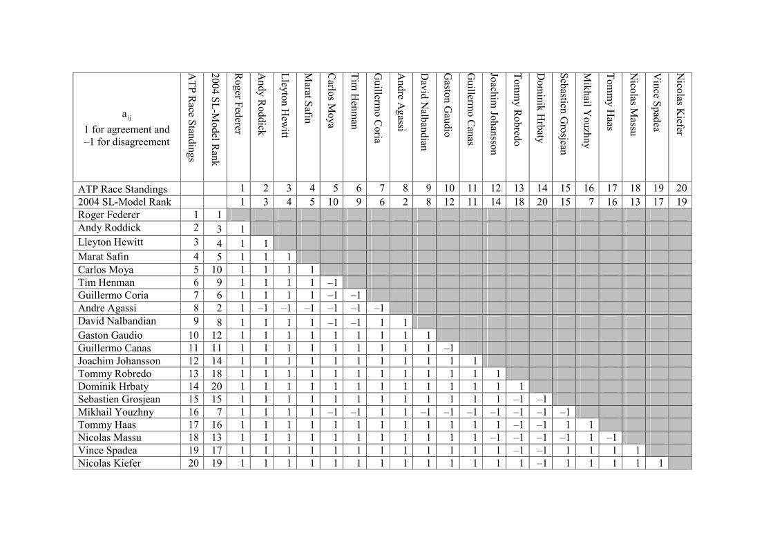
ija

1 for agreement and

–1 for disagreement

ATP Race S

tandings

2004 SL-M

odel R

ank

Roger F

ederer

Andy Roddick

Lley

ton Hew

itt

Marat S

afin

Carlo

s Moya

Tim

Henman

Guillerm

o Coria

Andre A

gassi

David Nalb

andian

Gasto

n Gaudio

Guillerm

o Canas

Joach

im Jo

hansso

n

Tommy Robred

o

Dominik Hrbaty

Sebastien

Grosjean

Mikhail Y

ouzhny

Tommy Haas

Nico

las Massu

Vince S

padea

Nico

las Kiefer

ATP Race Standings 1 2 3 4 5 6 7 8 9 10 11 12 13 14 15 16 17 18 19 20

2004 SL-Model Rank 1 3 4 5 10 9 6 2 8 12 11 14 18 20 15 7 16 13 17 19

Roger Federer 1 1

Andy Roddick 2 3 1

Lleyton Hewitt 3 4 1 1

Marat Safin 4 5 1 1 1

Carlos Moya 5 10 1 1 1 1

Tim Henman 6 9 1 1 1 1 –1

Guillermo Coria 7 6 1 1 1 1 –1 –1

Andre Agassi 8 2 1 –1 –1 –1 –1 –1 –1

David Nalbandian 9 8 1 1 1 1 –1 –1 1 1

Gaston Gaudio 10 12 1 1 1 1 1 1 1 1 1

Guillermo Canas 11 11 1 1 1 1 1 1 1 1 1 –1

Joachim Johansson 12 14 1 1 1 1 1 1 1 1 1 1 1

Tommy Robredo 13 18 1 1 1 1 1 1 1 1 1 1 1 1

Dominik Hrbaty 14 20 1 1 1 1 1 1 1 1 1 1 1 1 1

Sebastien Grosjean 15 15 1 1 1 1 1 1 1 1 1 1 1 1 –1 –1

Mikhail Youzhny 16 7 1 1 1 1 –1 –1 1 1 –1 –1 –1 –1 –1 –1 –1

Tommy Haas 17 16 1 1 1 1 1 1 1 1 1 1 1 1 –1 –1 1 1

Nicolas Massu 18 13 1 1 1 1 1 1 1 1 1 1 1 –1 –1 –1 –1 1 –1

Vince Spadea 19 17 1 1 1 1 1 1 1 1 1 1 1 1 –1 –1 1 1 1 1

Nicolas Kiefer 20 19 1 1 1 1 1 1 1 1 1 1 1 1 1 –1 1 1 1 1 1

85

We let:

−=

jobject and iobject of rankings twoin thent disagreeme if1

jobject and iobject of rankings twoin theagreement if1a ij ,

then we get the results seen on the previous table and we can calculate τ as ∑

∑

<

<

ji

2

ij

ji

ij

a

a

.

τ = 0.65263158

Test of significance based on Kendal’s Tau:



σ2 = 950

S = 124

z = 4.02309124

α = 0.95

Critical Value = ± 1.96

Reject H0.

At a 5% significance level there is sufficient evidence to say that there is an association

between the ranks obtained by the general SL-model on the 2004 data, and the ATP ranks.

86

Player

ATP Race

Standings For

11/22/04

2004 SL-

Model

Rank

Squared difference

of the ranks

2

id

Federer, Roger 1 1 0

Roddick, Andy 2 3 1

Hewitt, Lleyton 3 4 1

Safin, Marat 4 5 1

Moya, Carlos 5 10 25

Henman, Tim 6 9 9

Coria, Guillermo 7 6 1

Agassi, Andre 8 2 36

Nalbandian, David 9 8 1

Gaudio, Gaston 10 12 4

Canas, Guillermo 11 11 0

Johansson, Joachim 12 14 4

Robredo, Tommy 13 18 25

Hrbaty, Dominik 14 20 36

Grosjean, Sebastien 15 15 0

Youzhny, Mikhail 16 7 81

Haas, Tommy 17 16 1

Massu, Nicolas 18 13 25

Spadea, Vincent 19 17 4

Kiefer, Nicolas 20 19 1

Total 256

ρ = 0.807519

nn

d6

13

n

1i

2

i

−−=ρ∑= = 0.807519

87

Test of significance based on Spearman’s Rho:



σ2 = 0.052632

z = 3.519893

α = 0.95


Reject H0.


between the ranks obtained by the general SL-model on the 2004 data, and the ATP ranks.

We thus see that the test for association between the general SL-model ranks and the official

ranks using Kendal's τ and the test using Spearman's ρ both indicated an association between

the two sets of ranks. The value of τ was not that high, so we decided to investigate if it is

perhaps due to the official ranks possibly give more weight to more recent tournaments. We

thus did the same analysis on the data from the tournaments from the first half of the year and

that of the second half of the year. Again, the data using cumulative scores was calculated but

this time just from tournaments from the first half of 2004.

Cumulative score of ↓

when playing against

→

(First half of 2004)

Roger F

ederer

Andy Roddick

Lley

ton Hew

itt

Marat S

afin

Carlo

s Moya

Tim

Henman

Guillerm

o Coria

Andre A

gassi

David Nalb

andian

Gasto

n Gaudio

Guillerm

o Canas

Joach

im Jo

hansso

n

Tommy Robred

o

Dominik Hrbaty

Sebastien

Grosjean

Mikhail Y

ouzhny

Tommy Haas

Nico

las Massu

Vince S

padea

Nico

las Kiefer

Roger Federer 0 24 58 33 12 21 22 16 24 17 0 0 12 0 19 12 0 0 0 19

Andy Roddick 21 0 13 31 18 16 18 0 0 0 19 13 0 0 13 0 0 0 26 0

Lleyton Hewitt 29 9 0 0 27 12 0 0 0 21 0 0 0 0 0 0 13 0 0 0

Marat Safin 24 35 0 0 0 0 13 26 19 0 0 0 16 0 14 0 0 8 17 0

Carlos Moya 7 14 21 0 0 0 19 0 18 8 0 0 43 14 0 0 0 0 0 0

Tim Henman 19 19 6 0 0 0 15 0 0 0 32 0 13 0 0 0 0 15 19 0

Guillermo Coria 15 11 0 13 32 22 0 9 12 23 0 0 13 0 16 13 0 0 0 37

Andre Agassi 13 0 0 28 0 0 13 0 0 0 0 0 0 12 8 13 0 0 0 0


Gaston Gaudio 12 0 31 0 12 0 23 0 19 0 31 0 39 6 0 0 0 0 0 0

Guillermo Canas 0 19 0 0 0 34 0 0 7 31 0 0 16 0 0 0 13 0 0 0


Tommy Robredo 7 0 0 18 21 7 10 0 0 36 15 0 0 0 0 0 0 18 0 0

Dominik Hrbaty 0 0 0 0 14 0 0 6 3 19 0 0 0 0 14 7 0 0 0 0


Mikhail Youzhny 3 0 0 0 0 0 16 7 0 0 0 0 0 12 10 0 0 0 0 18

Tommy Haas 0 0 9 0 0 0 0 0 0 0 7 0 0 0 0 0 0 0 12 0

Nicolas Massu 0 0 0 13 0 13 0 0 0 0 0 0 4 0 0 0 0 0 0 0

Vince Spadea 0 22 0 19 0 17 0 0 7 0 0 0 0 0 0 0 12 0 0 19

Nicolas Kiefer 13 0 0 0 0 0 18 0 0 0 0 23 0 0 12 13 0 0 15 0

89

The weights and ranks obtained using the general SL-model for the data from the first half of

2004 was calculated as before in Mathematica.

Y={{0,24,58,33,12,21,22,16,24,17,0,0,12,0,19,12,0,0,0,19},{21,0,13,31,18,16,18,0,0,0,19,13,0,0,13,0,0,0,26,0},{29,9,0,0,27,12,0,0,0,21,0,0,0,0,0,0,13,0,0,0},{24,35,0,0,0,0,13,26,19,0,0,0,16,0,14,0,0,8,17,0},{7,14,21,0,0,0,19,0,18,8,0,0,43,14,0,0,0,0,0,0},{19,19,6,0,0,0,15,0,0,0,32,0,13,0,0,0,0,15,19,0},{15,11,0,13,32,22,0,9,12,23,0,0,13,0,16,13,0,0,0,37},{13,0,0,28,0,0,13,0,0,0,0,0,0,12,8,13,0,0,0,0},{19,0,0,25,7,0,7,0,0,9,18,0,0,12,0,0,0,0,12,0},{12,0,31,0,12,0,23,0,19,0,31,0,39,6,0,0,0,0,0,0},{0,19,0,0,0,34,0,0,7,31,0,0,16,0,0,0,13,0,0,0},{0,9,0,0,0,0,0,0,0,0,0,0,0,0,0,0,0,0,0,31},{7,0,0,18,21,7,10,0,0,36,15,0,0,0,0,0,0,18,0,0},{0,0,0,0,14,0,0,6,3,19,0,0,0,0,14,7,0,0,0,0},{11,10,0,11,0,0,14,2,0,0,0,0,0,20,0,19,0,0,0,6},{3,0,0,0,0,0,16,7,0,0,0,0,0,12,10,0,0,0,0,18},{0,0,9,0,0,0,0,0,0,0,7,0,0,0,0,0,0,0,12,0},{0,0,0,13,0,13,0,0,0,0,0,0,4,0,0,0,0,0,0,0},{0,22,0,19,0,17,0,0,7,0,0,0,0,0,0,0,12,0,0,19},{13,0,0,0,0,0,18,0,0,0,0,23,0,0,12,13,0,0,15,0}}

y[i_,j_]:=Extract[Y,{i,j}] l[i_,j_]:=y[i,j]/(p[i]+1-p[j]) r[i_,j_]:=l[j,i] s[i_,j_]:=l[i,j]-r[i,j] e[i_]:=Sum[s[i,j],{j,1,20}] FindRoot[Table[e[i]�0,{i,1,20}],Table[{p[i],0.5},{i,1,20}]]

{p[1]→0.841649,p[2]→0.701305,p[3]→0.596944,p[4]→0.640939,p[5]

→0.652591,p[6]→0.638365,p[7]→0.717001,p[8]→0.806532,p[9]→0.68

109,p[10]→0.668278,p[11]→0.628319,p[12]→0.611016,p[13]→0.5720

68,p[14]→0.559451,p[15]→0.594409,p[16]→0.570753,p[17]→0.45036

6,p[18]→0.46682,p[19]→0.585877,p[20]→0.5}

90

Thus the following results were obtained:

ATP Race

Standings

For


1st half of

2004 SL-

Model

Weight

1st half of

2004 SL-

Model

Rank





















As before, we then went on to calculate Kendal's τ and Spearman's ρ and used them to test

the association between the general SL-model (using just 1st half of 2004 data) ranks and the

official ranks.

ija

1 for agreement and


ATP Race S

tandings

1st h

alf of 2

004 SL-M

odel

Rank

Roger F

ederer

Andy Roddick

Lley

ton Hew

itt

Marat S

afin

Carlo

s Moya

Tim

Henman

Guillerm

o Coria

Andre A

gassi

David Nalb

andian

Gasto

n Gaudio

Guillerm

o Canas

Joach

im Jo

hansso

n

Tommy Robred

o

Dominik Hrbaty

Sebastien

Grosjean

Mikhail Y

ouzhny

Tommy Haas

Nico

las Massu

Vince S

padea

Nico

las Kiefer


1st half of 2004 SL-

Model Rank

1 4 12 8 7 9 3 2 5 6 10 11 15 17 13 16 20 19 14 18

Roger Federer 1 1

Andy Roddick 2 4 1


Marat Safin 4 8 1 1 –1

Carlos Moya 5 7 1 1 –1 –1

Tim Henman 6 9 1 1 –1 1 1

Guillermo Coria 7 3 1 –1 –1 –1 –1 –1

Andre Agassi 8 2 1 –1 –1 –1 –1 –1 –1

David Nalbandian 9 5 1 1 –1 –1 –1 –1 1 1

Gaston Gaudio 10 6 1 1 –1 –1 –1 –1 1 1 1

Guillermo Canas 11 10 1 1 –1 1 1 1 1 1 1 1

Joachim Johansson 12 11 1 1 –1 1 1 1 1 1 1 1 1

Tommy Robredo 13 15 1 1 1 1 1 1 1 1 1 1 1 1

Dominik Hrbaty 14 17 1 1 1 1 1 1 1 1 1 1 1 1 1


Mikhail Youzhny 16 16 1 1 1 1 1 1 1 1 1 1 1 1 1 –1 1

Tommy Haas 17 20 1 1 1 1 1 1 1 1 1 1 1 1 1 1 1 1

Nicolas Massu 18 19 1 1 1 1 1 1 1 1 1 1 1 1 1 1 1 1 –1

Vince Spadea 19 14 1 1 1 1 1 1 1 1 1 1 1 1 –1 –1 1 –1 –1 –1

Nicolas Kiefer 20 18 1 1 1 1 1 1 1 1 1 1 1 1 1 1 1 1 –1 –1 1

92

−=



τ =∑

∑

<

<

ji

2

ij

ji

ij

a

a

= 0.621053




σ2 = 950

S = 118

z = 3.828426

α = 0.95


Reject H0.


between the ranks obtained by the general SL-model on the first half of 2004 data, and the

ATP ranks.

93

Player

ATP Race

Standings For

11/22/04

1st half of

2004 SL-

Model Rank

Squared

difference of

the ranks


Roddick, Andy 2 4 4


Safin, Marat 4 8 16

Moya, Carlos 5 7 4

Henman, Tim 6 9 9











Haas, Tommy 17 20 9




Total 256

ρ = 0.807519

nn

d6

13

n

1i

2

i

−−=ρ∑= = 0.807519

94




σ2 = 0.052632

z = 3.519893

α = 0.95


Reject H0.


between the ranks obtained by the general SL-model on the first half of 2004 data, and the

ATP ranks.

The cumulative scores were calculated from tournaments from the second half of 2004, as

seen on the next page.

Cumulative score of ↓

when playing against

→

(Second half of 2004)

Roger F

ederer

Andy Roddick

Lley

ton Hew

itt

Marat S

afin

Carlo

s Moya

Tim

Henman

Guillerm

o Coria

Andre A

gassi

David Nalb

andian

Gasto

n Gaudio

Guillerm

o Canas

Joach

im Jo

hansso

n

Tommy Robred

o

Dominik Hrbaty

Sebastien

Grosjean

Mikhail Y

ouzhny

Tommy Haas

Nico

las Massu

Vince S

padea

Nico

las Kiefer

Roger Federer 0 25 43 13 15 18 0 24 0 13 0 0 0 16 0 0 0 0 0 0

Andy Roddick 12 0 5 34 0 14 13 18 0 0 18 24 18 12 0 0 31 0 0 37

Lleyton Hewitt 18 12 0 22 18 12 0 11 0 12 0 19 12 0 0 0 18 4 0 0

Marat Safin 9 31 21 0 0 13 12 13 18 0 13 0 0 0 0 14 0 0 0 17

Carlos Moya 12 0 13 0 0 0 0 9 0 12 0 0 0 0 0 0 0 7 0 14

Tim Henman 11 11 5 8 0 0 12 0 0 0 0 0 0 24 0 6 0 0 0 27

Guillermo Coria 0 9 0 5 0 4 0 0 0 0 0 0 0 0 0 0 0 0 0 0

Andre Agassi 23 20 15 9 13 0 0 0 0 0 0 0 18 0 0 0 46 0 12 0


Gaston Gaudio 7 0 3 0 7 0 0 0 0 0 18 0 0 0 0 0 0 10 0 0

Guillermo Canas 0 7 0 8 0 0 0 0 14 24 0 11 0 0 0 0 25 0 0 0


Tommy Robredo 0 9 5 0 0 0 0 12 0 0 0 0 0 0 0 0 0 0 0 0

Dominik Hrbaty 7 5 0 0 0 15 0 0 0 0 0 18 0 0 0 6 0 0 0 14


Mikhail Youzhny 0 0 0 11 0 13 0 0 42 0 0 0 0 12 0 0 0 15 0 15

Tommy Haas 0 22 6 0 0 0 0 45 0 0 15 0 0 0 19 0 0 0 0 13

Nicolas Massu 0 0 3 0 13 0 0 0 7 13 0 0 0 0 0 12 0 0 13 0

Vince Spadea 0 0 0 0 0 0 0 4 8 0 0 0 0 0 0 0 0 8 0 0

Nicolas Kiefer 0 21 0 19 14 18 0 0 0 0 0 13 0 17 0 10 10 0 0 0

96

The weights and ranks obtained using the general SL-model for this data was calculated as

before in Mathematica.

Y={{0,25,43,13,15,18,0,24,0,13,0,0,0,16,0,0,0,0,0,0},{12,0,5,34,0,14,13,18,0,0,18,24,18,12,0,0,31,0,0,37},{18,12,0,22,18,12,0,11,0,12,0,19,12,0,0,0,18,4,0,0},{9,31,21,0,0,13,12,13,18,0,13,0,0,0,0,14,0,0,0,17},{12,0,13,0,0,0,0,9,0,12,0,0,0,0,0,0,0,7,0,14},{11,11,5,8,0,0,12,0,0,0,0,0,0,24,0,6,0,0,0,27},{0,9,0,5,0,4,0,0,0,0,0,0,0,0,0,0,0,0,0,0},{23,20,15,9,13,0,0,0,0,0,0,0,18,0,0,0,46,0,12,0},{0,0,0,9,0,0,0,0,0,0,13,0,0,0,0,39,0,12,12,0},{7,0,3,0,7,0,0,0,0,0,18,0,0,0,0,0,0,10,0,0},{0,7,0,8,0,0,0,0,14,24,0,11,0,0,0,0,25,0,0,0},{0,23,12,0,0,0,0,0,0,0,14,0,0,18,0,0,0,0,0,9},{0,9,5,0,0,0,0,12,0,0,0,0,0,0,0,0,0,0,0,0},{7,5,0,0,0,15,0,0,0,0,0,18,0,0,0,6,0,0,0,14},{0,0,0,0,0,0,0,0,0,0,0,0,0,0,0,0,15,0,0,0},{0,0,0,11,0,13,0,0,42,0,0,0,0,12,0,0,0,15,0,15},{0,22,6,0,0,0,0,45,0,0,15,0,0,0,19,0,0,0,0,13},{0,0,3,0,13,0,0,0,7,13,0,0,0,0,0,12,0,0,13,0},{0,0,0,0,0,0,0,4,8,0,0,0,0,0,0,0,0,8,0,0},{0,21,0,19,14,18,0,0,0,0,0,13,0,17,0,10,10,0,0,0}}


{p[1]→0.865971,p[2]→0.668329,p[3]→0.729157,p[4]→0.702211,p[5]

→0.54826,p[6]→0.57944,p[7]→0.311334,p[8]→0.667698,p[9]→0.5716

52,p[10]→0.377549,p[11]→0.52114,p[12]→0.519568,p[13]→0.384071

,p[14]→0.404215,p[15]→0.38898,p[16]→0.670224,p[17]→0.506627,p

[18]→0.553494,p[19]→0.291035,p[20]→0.5}

97

The following results were obtained:

ATP Race

Standings For


2nd half of

2004 SL-Model

Weight

2nd half of

2004 SL-

Model Rank





















We then again went on to calculate Kendal's τ and Spearman's ρ and used them to test the

association between the general SL-model (using just 2nd half of 2004 data) ranks and the

official ranks.

ija

1 for agreement and


ATP Race S

tandings

2nd half o

f 2004 SL-

Model R

ank

Roger F

ederer

Andy Roddick

Lley

ton Hew

itt

Marat S

afin

Carlo

s Moya

Tim

Henman

Guillerm

o Coria

Andre A

gassi

David Nalb

andian

Gasto

n Gaudio

Guillerm

o Canas

Joach

im Jo

hansso

n

Tommy Robred

o

Dominik Hrbaty

Sebastien

Grosjean

Mikhail Y

ouzhny

Tommy Haas

Nico

las Massu

Vince S

padea

Nico

las Kiefer


2nd half of 2004 SL-

Model Rank

1 5 2 3 10 7 19 6 8 18 11 12 17 15 16 4 13 9 20 14

Roger Federer 1 1

Andy Roddick 2 5 1

Lleyton Hewitt 3 2 1 –1

Marat Safin 4 3 1 –1 1


Tim Henman 6 7 1 1 1 1 –1

Guillermo Coria 7 19 1 1 1 1 1 1

Andre Agassi 8 6 1 1 1 1 –1 –1 –1

David Nalbandian 9 8 1 1 1 1 –1 1 –1 1

Gaston Gaudio 10 18 1 1 1 1 1 1 –1 1 1

Guillermo Canas 11 11 1 1 1 1 1 1 –1 1 1 –1

Joachim Johansson 12 12 1 1 1 1 1 1 –1 1 1 –1 1

Tommy Robredo 13 17 1 1 1 1 1 1 –1 1 1 –1 1 1

Dominik Hrbaty 14 15 1 1 1 1 1 1 –1 1 1 –1 1 1 –1

Sebastien Grosjean 15 16 1 1 1 1 1 1 –1 1 1 –1 1 1 –1 1

Mikhail Youzhny 16 4 1 –1 1 1 –1 –1 –1 –1 –1 –1 –1 –1 –1 –1 –1

Tommy Haas 17 13 1 1 1 1 1 1 –1 1 1 –1 1 1 –1 –1 –1 1

Nicolas Massu 18 9 1 1 1 1 –1 1 –1 1 1 –1 –1 –1 –1 –1 –1 1 –1

Vince Spadea 19 20 1 1 1 1 1 1 1 1 1 1 1 1 1 1 1 1 1 1

Nicolas Kiefer 20 14 1 1 1 1 1 1 –1 1 1 –1 1 1 –1 –1 –1 1 1 1 –1

99

−=



τ =∑

∑

<

<

ji

2

ij

ji

ij

a

a

= 0.442105




σ2 = 950

S = 84

z = 2.72532

α = 0.95


Reject H0.


between the ranks obtained by the general SL-model on the second half of 2004 data, and the

ATP ranks.

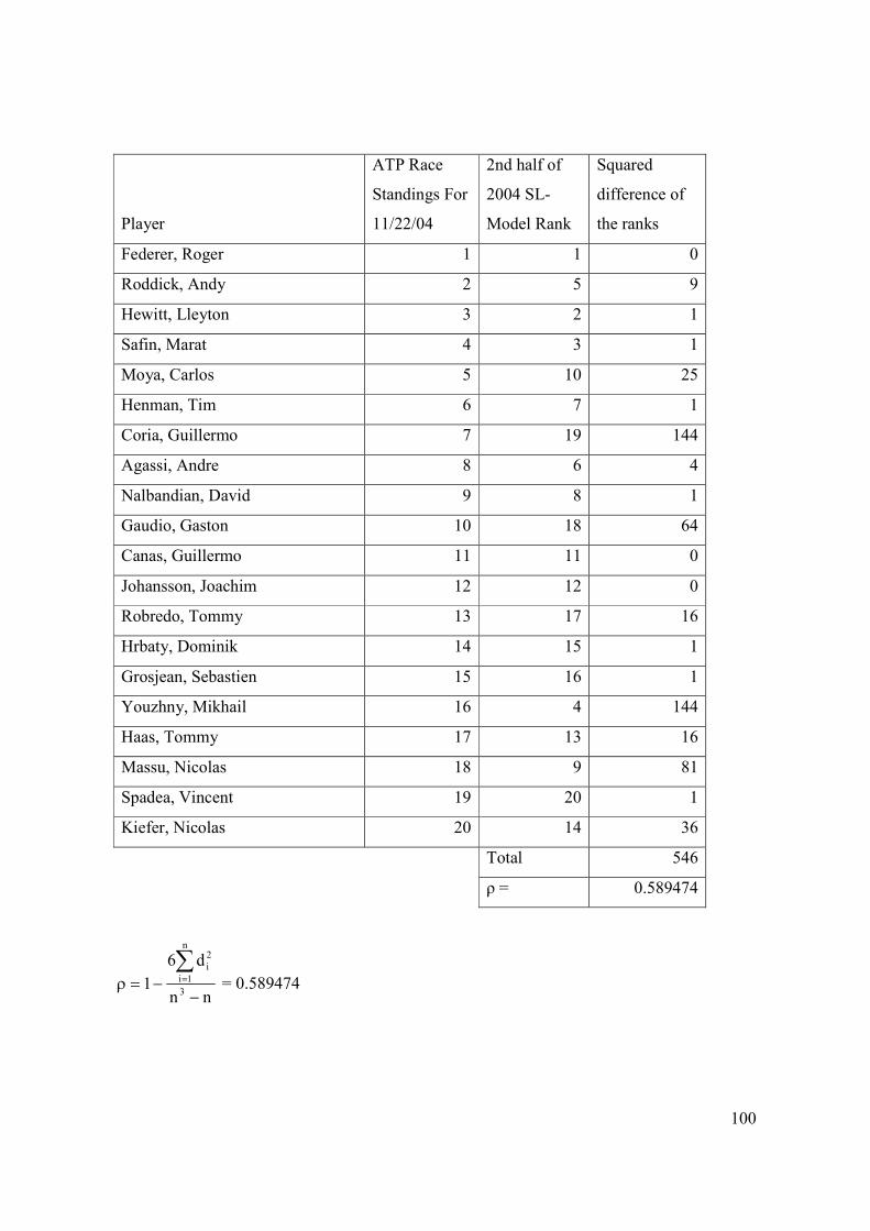
100

Player

ATP Race

Standings For

11/22/04

2nd half of

2004 SL-

Model Rank

Squared

difference of

the ranks


Roddick, Andy 2 5 9


Safin, Marat 4 3 1


Henman, Tim 6 7 1


Agassi, Andre 8 6 4









Haas, Tommy 17 13 16




Total 546

ρ = 0.589474

nn

d6

13

n

1i

2

i

−−=ρ∑= = 0.589474

101




σ2 = 0.052632

z = 2.569456

α = 0.95


Reject H0.


between the ranks obtained by the general SL-model on the second half of 2004 data, and the

ATP ranks.

We thus found that the data from the first half of the year had a stronger association with the

official ranks than the data from the second half of the year, which is the opposite to what

should occur if the official ranks gave more weight to more recent tournaments, so we

concluded that that was not the reason why our measure of association was not higher.

7.4 Real Life Application of the Binary SL-Model

Even though the tests conclude that there is an association between the SL-model ranks and

the official ranks, the measures of association are not that good, especially for data from the

second half of the year. We then decided to simply use cumulative number of wins in our

model, instead of cumulative scores, as sometimes ranks of players are calculated in this

manner. We called this the binary SL-model (bin SL-model) as score is 1 if a team wins and

0 if it looses.

The data for 2004 for cumulative number of wins was thus summarised on the next page:

Cumulative number of

wins of ↓ when playing

against →

(2004)

Roger F

ederer

Andy Roddick

Lley

ton Hew

itt

Marat S

afin

Carlo

s Moya

Tim

Henman

Guillerm

o Coria

Andre A

gassi

David Nalb

andian

Gasto

n Gaudio

Guillerm

o Canas

Joach

im Jo

hansso

n

Tommy Robred

o

Dominik Hrbaty

Sebastien

Grosjean

Mikhail Y

ouzhny

Tommy Haas

Nico

las Massu

Vince S

padea

Nico

las Kiefer

Roger Federer 0 7 15 7 4 5 3 5 3 4 0 0 2 1 3 2 0 0 0 3

Andy Roddick 1 0 2 8 2 3 4 1 0 0 5 4 3 2 2 0 4 0 3 6

Lleyton Hewitt 2 2 0 2 6 4 0 1 0 4 0 3 2 0 0 0 5 1 0 0

Marat Safin 0 4 2 0 0 2 3 5 4 0 2 0 2 0 2 2 0 0 1 1

Carlos Moya 1 1 2 0 0 0 0 0 3 2 0 0 7 2 0 0 0 0 0 1

Tim Henman 2 2 0 0 0 0 3 0 0 0 2 0 2 3 0 0 0 2 2 3

Guillermo Coria 1 1 0 2 5 3 0 0 2 2 0 0 2 0 2 1 0 0 0 6

Andre Agassi 3 2 2 2 2 0 2 0 0 0 0 0 2 2 2 2 5 0 2 0


Gaston Gaudio 1 0 4 0 2 0 3 0 3 0 5 0 5 0 0 0 0 0 0 0

Guillermo Canas 0 2 0 0 0 3 0 0 2 7 0 0 1 0 0 0 6 0 0 0


Tommy Robredo 0 0 0 1 0 0 0 1 0 3 2 0 0 0 0 0 0 3 0 0

Dominik Hrbaty 2 0 0 0 1 1 0 0 0 3 0 2 0 0 1 0 0 0 0 1


Mikhail Youzhny 0 0 0 0 0 2 2 0 5 0 0 0 0 4 0 0 0 2 0 4

Tommy Haas 0 1 0 0 0 0 0 3 0 0 0 0 0 0 3 0 0 0 1 2

Nicolas Massu 0 0 0 2 2 1 0 0 0 2 0 0 0 0 0 1 0 0 2 0

Vince Spadea 0 2 0 2 0 1 0 0 0 0 0 0 0 0 0 0 2 0 0 2

Nicolas Kiefer 0 0 0 2 2 2 0 0 0 0 0 3 0 2 2 2 0 0 1 0

103

From the cumulative number of wins for 2004 the weights and ranks obtained using the SL-

model for this data was calculated as before in Mathematica.


{p[1]→1.11731,p[2]→0.760563,p[3]→0.712574,p[4]→0.516633,p[5]→

0.365933,p[6]→0.426267,p[7]→0.596503,p[8]→0.730478,p[9]→0.417

469,p[10]→0.395205,p[11]→0.372021,p[12]→0.340322,p[13]→0.0000

678147,p[14]→0.293066,p[15]→0.0495587,p[16]→0.428695,p[17]→0.

115443,p[18]→0.327698,p[19]→0.181146,p[20]→0.0541}

104


ATP Race

Standings For


2004 Bin SL-

Model Weight

2004 Bin SL-

Model Rank













13 Robredo, Tommy ESP 6.7815E-05 20









association between the binary SL-model ranks and the official ranks.

ija

1 for agreement and


ATP Race S

tandings

2004 Bin SL-M

odel

Rank

Roger F

ederer

Andy Roddick

Lley

ton Hew

itt

Marat S

afin

Carlo

s Moya

Tim

Henman

Guillerm

o Coria

Andre A

gassi

David Nalb

andian

Gasto

n Gaudio

Guillerm

o Canas

Joach

im Jo

hansso

n

Tommy Robred

o

Dominik Hrbaty

Sebastien

Grosjean

Mikhail Y

ouzhny

Tommy Haas

Nico

las Massu

Vince S

padea

Nico

las Kiefer


2004 Bin SL-Model

Rank

1 2 4 6 12 8 5 3 9 10 11 13 20 15 19 7 17 14 16 18

Roger Federer 1 1

Andy Roddick 2 2 1




Tim Henman 6 8 1 1 1 1 –1

Guillermo Coria 7 5 1 1 1 –1 –1 –1

Andre Agassi 8 3 1 1 –1 –1 –1 –1 –1

David Nalbandian 9 9 1 1 1 1 –1 1 1 1

Gaston Gaudio 10 10 1 1 1 1 –1 1 1 1 1

Guillermo Canas 11 11 1 1 1 1 –1 1 1 1 1 1


Tommy Robredo 13 20 1 1 1 1 1 1 1 1 1 1 1 1

Dominik Hrbaty 14 15 1 1 1 1 1 1 1 1 1 1 1 1 –1

Sebastien Grosjean 15 19 1 1 1 1 1 1 1 1 1 1 1 1 –1 1

Mikhail Youzhny 16 7 1 1 1 1 –1 –1 1 1 –1 –1 –1 –1 –1 –1 –1

Tommy Haas 17 17 1 1 1 1 1 1 1 1 1 1 1 1 –1 1 –1 1

Nicolas Massu 18 14 1 1 1 1 1 1 1 1 1 1 1 1 –1 –1 –1 1 –1

Vince Spadea 19 16 1 1 1 1 1 1 1 1 1 1 1 1 –1 1 –1 1 –1 1

Nicolas Kiefer 20 18 1 1 1 1 1 1 1 1 1 1 1 1 –1 1 –1 1 1 1 1

106

−=



τ =∑

∑

<

<

ji

2

ij

ji

ij

a

a

= 0.64210526




σ2 = 950

S = 122

z = 3.95820268

α = 0.95


Reject H0.


between the ranks obtained by the binary SL-model on the 2004 data, and the ATP ranks.

107

Player

ATP Race

Standings For

11/22/04

2004 Bin SL-

Model Rank

Squared

difference of

the ranks


Roddick, Andy 2 2 0


Safin, Marat 4 6 4


Henman, Tim 6 8 4











Haas, Tommy 17 17 0




Total 264

ρ = 0.801504

nn

d6

13

n

1i

2

i

−−=ρ∑= = 0.801504

108




σ2 = 0.052632

z = 3.493674

α = 0.95


Reject H0.


between the ranks obtained by the binary SL-model on the 2004 data, and the ATP ranks.

We however noticed that these measures of association using cumulative number of wins is

slightly less than that using cumulative scores. We also found that the weights of the objects

were not all between 0 and 1, as required by theorem 4 to get proper probabilities. This could

be because the data contains too many zeros in it.

We then proceeded to do the same analysis on the cumulative number of wins from the first

half of the year and the cumulative number of wins from the second half of the year.



against →

(first half of 2004)

Roger F

ederer

Andy Roddick

Lley

ton Hew

itt

Marat S

afin

Carlo

s Moya

Tim

Henman

Guillerm

o Coria

Andre A

gassi

David Nalb

andian

Gasto

n Gaudio

Guillerm

o Canas

Joach

im Jo

hansso

n

Tommy Robred

o

Dominik Hrbaty

Sebastien

Grosjean

Mikhail Y

ouzhny

Tommy Haas

Nico

las Massu

Vince S

padea

Nico

las Kiefer

Roger Federer 0 3 8 5 2 2 3 2 3 2 0 0 2 0 3 2 0 0 0 3

Andy Roddick 1 0 2 4 2 1 2 0 0 0 2 2 0 0 2 0 0 0 3 0

Lleyton Hewitt 2 0 0 0 4 2 0 0 0 2 0 0 0 0 0 0 2 0 0 0

Marat Safin 0 3 0 0 0 0 1 3 1 0 0 0 2 0 2 0 0 0 1 0

Carlos Moya 0 1 1 0 0 0 0 0 3 0 0 0 7 2 0 0 0 0 0 0

Tim Henman 2 2 0 0 0 0 1 0 0 0 2 0 2 0 0 0 0 2 2 0

Guillermo Coria 1 1 0 2 5 3 0 0 2 2 0 0 2 0 2 1 0 0 0 6

Andre Agassi 1 0 0 2 0 0 2 0 0 0 0 0 0 2 2 2 0 0 0 0


Gaston Gaudio 1 0 4 0 2 0 3 0 3 0 3 0 5 0 0 0 0 0 0 0

Guillermo Canas 0 2 0 0 0 3 0 0 0 4 0 0 1 0 0 0 2 0 0 0


Tommy Robredo 0 0 0 1 0 0 0 0 0 3 2 0 0 0 0 0 0 3 0 0

Dominik Hrbaty 0 0 0 0 1 0 0 0 0 3 0 0 0 0 1 0 0 0 0 0


Mikhail Youzhny 0 0 0 0 0 0 2 0 0 0 0 0 0 2 0 0 0 0 0 2

Tommy Haas 0 0 0 0 0 0 0 0 0 0 0 0 0 0 0 0 0 0 1 0

Nicolas Massu 0 0 0 2 0 1 0 0 0 0 0 0 0 0 0 0 0 0 0 0

Vince Spadea 0 2 0 2 0 1 0 0 0 0 0 0 0 0 0 0 2 0 0 2

Nicolas Kiefer 0 0 0 0 0 0 0 0 0 0 0 1 0 0 2 1 0 0 1 0



against →

(second half of 2004)

Roger F

ederer

Andy Roddick

Lley

ton Hew

itt

Marat S

afin

Carlo

s Moya

Tim

Henman

Guillerm

o Coria

Andre A

gassi

David Nalb

andian

Gasto

n Gaudio

Guillerm

o Canas

Joach

im Jo

hansso

n

Tommy Robred

o

Dominik Hrbaty

Sebastien

Grosjean

Mikhail Y

ouzhny

Tommy Haas

Nico

las Massu

Vince S

padea

Nico

las Kiefer

Roger Federer 0 4 7 2 2 3 0 3 0 2 0 0 0 1 0 0 0 0 0 0

Andy Roddick 0 0 0 4 0 2 2 1 0 0 3 2 3 2 0 0 4 0 0 6

Lleyton Hewitt 0 2 0 2 2 2 0 1 0 2 0 3 2 0 0 0 3 1 0 0

Marat Safin 0 1 2 0 0 2 2 2 3 0 2 0 0 0 0 2 0 0 0 1

Carlos Moya 1 0 1 0 0 0 0 0 0 2 0 0 0 0 0 0 0 0 0 1

Tim Henman 0 0 0 0 0 0 2 0 0 0 0 0 0 3 0 0 0 0 0 3

Guillermo Coria 0 0 0 0 0 0 0 0 0 0 0 0 0 0 0 0 0 0 0 0

Andre Agassi 2 2 2 0 2 0 0 0 0 0 0 0 2 0 0 0 5 0 2 0


Gaston Gaudio 0 0 0 0 0 0 0 0 0 0 2 0 0 0 0 0 0 0 0 0

Guillermo Canas 0 0 0 0 0 0 0 0 2 3 0 0 0 0 0 0 4 0 0 0


Tommy Robredo 0 0 0 0 0 0 0 1 0 0 0 0 0 0 0 0 0 0 0 0

Dominik Hrbaty 2 0 0 0 0 1 0 0 0 0 0 2 0 0 0 0 0 0 0 1


Mikhail Youzhny 0 0 0 0 0 2 0 0 5 0 0 0 0 2 0 0 0 2 0 2

Tommy Haas 0 1 0 0 0 0 0 3 0 0 0 0 0 0 3 0 0 0 0 2

Nicolas Massu 0 0 0 0 2 0 0 0 0 2 0 0 0 0 0 1 0 0 2 0

Vince Spadea 0 0 0 0 0 0 0 0 0 0 0 0 0 0 0 0 0 0 0 0

Nicolas Kiefer 0 0 0 2 2 2 0 0 0 0 0 2 0 2 0 1 0 0 0 0

111

The weights and ranks obtained using the SL-model on cumulative number of wins (i.e.

Binary SL-Model) for the data from the first half of 2004 and that of the second half of 2004

respectively was calculated as before in Mathematica.

Y={{0,3,8,5,2,2,3,2,3,2,0,0,2,0,3,2,0,0,0,3},{1,0,2,4,2,1,2,0,

0,0,2,2,0,0,2,0,0,0,3,0},{2,0,0,0,4,2,0,0,0,2,0,0,0,0,0,0,2,0,

0,0},{0,3,0,0,0,0,1,3,1,0,0,0,2,0,2,0,0,0,1,0},{0,1,1,0,0,0,0,

0,3,0,0,0,7,2,0,0,0,0,0,0},{2,2,0,0,0,0,1,0,0,0,2,0,2,0,0,0,0,

2,2,0},{1,1,0,2,5,3,0,0,2,2,0,0,2,0,2,1,0,0,0,6},{1,0,0,2,0,0,

2,0,0,0,0,0,0,2,2,2,0,0,0,0},{1,0,0,3,0,0,0,0,0,0,3,0,0,2,0,0,

0,0,2,0},{1,0,4,0,2,0,3,0,3,0,3,0,5,0,0,0,0,0,0,0},{0,2,0,0,0,

3,0,0,0,4,0,0,1,0,0,0,2,0,0,0},{0,0,0,0,0,0,0,0,0,0,0,0,0,0,0,

0,0,0,0,4},{0,0,0,1,0,0,0,0,0,3,2,0,0,0,0,0,0,3,0,0},{0,0,0,0,

1,0,0,0,0,3,0,0,0,0,1,0,0,0,0,0},{0,0,0,0,0,0,1,0,0,0,0,0,0,3,

0,3,0,0,0,0},{0,0,0,0,0,0,2,0,0,0,0,0,0,2,0,0,0,0,0,2},{0,0,0,

0,0,0,0,0,0,0,0,0,0,0,0,0,0,0,1,0},{0,0,0,2,0,1,0,0,0,0,0,0,0,

0,0,0,0,0,0,0},{0,2,0,2,0,1,0,0,0,0,0,0,0,0,0,0,2,0,0,2},{0,0,

0,0,0,0,0,0,0,0,0,1,0,0,2,1,0,0,1,0}}

y[i_,j_]:=Extract[Y,{i,j}] l[i_,j_]:=y[i,j]/(p[i]+1-p[j]) r[i_,j_]:=l[j,i] s[i_,j_]:=l[i,j]-r[i,j] e[i_]:=Sum[s[i,j],{j,1,20}]

FindRoot[Table[e[i]�0,{i,1,20}],Table[{p[i],0.1047},{i,1,20}]]

{p[1]→1.76777,p[2]→1.20716,p[3]→1.17902,p[4]→0.876676,p[5]→0.

922572,p[6]→1.14342,p[7]→1.22699,p[8]→1.40502,p[9]→1.07541,p[

10]→1.08755,p[11]→0.988795,p[12]→0.507545,p[13]→0.577857,p[14

]→0.555997,p[15]→0.495449,p[16]→0.624965,p[17]→0.0000645822,p

[18]→0.648951,p[19]→0.679012,p[20]→0.1047}

112

Y={{0,4,7,2,2,3,0,3,0,2,0,0,0,1,0,0,0,0,0,0},{0,0,0,4,0,2,2,1,

0,0,3,2,3,2,0,0,4,0,0,6},{0,2,0,2,2,2,0,1,0,2,0,3,2,0,0,0,3,1,

0,0},{0,1,2,0,0,2,2,2,3,0,2,0,0,0,0,2,0,0,0,1},{1,0,1,0,0,0,0,

0,0,2,0,0,0,0,0,0,0,0,0,1},{0,0,0,0,0,0,2,0,0,0,0,0,0,3,0,0,0,

0,0,3},{0,0,0,0,0,0,0,0,0,0,0,0,0,0,0,0,0,0,0,0},{2,2,2,0,2,0,

0,0,0,0,0,0,2,0,0,0,5,0,2,0},{0,0,0,0,0,0,0,0,0,0,1,0,0,0,0,3,

0,2,2,0},{0,0,0,0,0,0,0,0,0,0,2,0,0,0,0,0,0,0,0,0},{0,0,0,0,0,

0,0,0,2,3,0,0,0,0,0,0,4,0,0,0},{0,3,0,0,0,0,0,0,0,0,2,0,0,1,0,

0,0,0,0,0},{0,0,0,0,0,0,0,1,0,0,0,0,0,0,0,0,0,0,0,0},{2,0,0,0,

0,1,0,0,0,0,0,2,0,0,0,0,0,0,0,1},{0,0,0,0,0,0,0,0,0,0,0,0,0,0,

0,0,1,0,0,0},{0,0,0,0,0,2,0,0,5,0,0,0,0,2,0,0,0,2,0,2},{0,1,0,

0,0,0,0,3,0,0,0,0,0,0,3,0,0,0,0,2},{0,0,0,0,2,0,0,0,0,2,0,0,0,

0,0,1,0,0,2,0},{0,0,0,0,0,0,0,0,0,0,0,0,0,0,0,0,0,0,0,0},{0,0,

0,2,2,2,0,0,0,0,0,2,0,2,0,1,0,0,0,0}}

y[i_,j_]:=Extract[Y,{i,j}]

l[i_,j_]:=y[i,j]/(p[i]+1-p[j])

r[i_,j_]:=l[j,i]

s[i_,j_]:=l[i,j]-r[i,j]

e[i_]:=Sum[s[i,j],{j,1,20}]


8p@1D → 1.36237, p@2D → 1.07141, p@3D → 1.13472, p@4D → 1.02549,

p@5D → 0.594295, p@6D → 0.274676, p@7D → −9.2152×106, p@8D → 0.860383,

p@9D → 0.397084, p@10D → −0.512893, p@11D → 0.104891, p@12D → 0.628258,

p@13D → 0.130653, p@14D → 0.618676, p@15D → −0.163415, p@16D → 0.811015,

p@17D → 0.336585, p@18D → 0.531816, p@19D → −9.25924×106, p@20D → 0.5<

113


ATP Race

Standings

For


1st half of

2004 Bin

SL-Model

Weight

1st half of

2004 Bin

SL-Model

Rank

2nd half of

2004 Bin SL-

Model

Weight

2nd half of

2004 Bin

SL-Model

Rank

1 Federer, Roger SUI 1.76777 1 1.36237 1

2 Roddick, Andy USA 1.20716 4 1.07141 3

3 Hewitt, Lleyton AUS 1.17902 5 1.13472 2

4 Safin, Marat RUS 0.876676 11 1.02549 4

5 Moya, Carlos ESP 0.922572 10 0.594295 9

6 Henman, Tim GBR 1.14342 6 0.274676 14

7 Coria, Guillermo ARG 1.22699 3 –9215199 19

8 Agassi, Andre USA 1.40502 2 0.860383 5

9 Nalbandian, David ARG 1.07541 8 0.397084 12

10 Gaudio, Gaston ARG 1.08755 7 –0.512893 18

11 Canas, Guillermo ARG 0.988795 9 0.104891 16

12 Johansson, Joachim SWE 0.507545 17 0.628258 7

13 Robredo, Tommy ESP 0.577857 15 0.130653 15

14 Hrbaty, Dominik SVK 0.555997 16 0.618676 8

15 Grosjean, Sebastien FRA 0.495449 18 –0.163415 17

16 Youzhny, Mikhail RUS 0.624965 14 0.811015 6

17 Haas, Tommy GER 6.4582E-05 20 0.336585 13

18 Massu, Nicolas CHI 0.648951 13 0.531816 10

19 Spadea, Vincent USA 0.679012 12 –9259244 20

20 Kiefer, Nicolas GER 0.1047 19 0.5 11


association between the binary SL-model ranks for the first half of the year and the official

ranks, and the association between the binary SL-model ranks for the second half of the year

and the official ranks.

ija

1 for agreement and


ATP Race S

tandings

1st h

alf of 2

004 Bin SL-

Model R

ank

Roger F

ederer

Andy Roddick

Lley

ton Hew

itt

Marat S

afin

Carlo

s Moya

Tim

Henman

Guillerm

o Coria

Andre A

gassi

David Nalb

andian

Gasto

n Gaudio

Guillerm

o Canas

Joach

im Jo

hansso

n

Tommy Robred

o

Dominik Hrbaty

Sebastien

Grosjean

Mikhail Y

ouzhny

Tommy Haas

Nico

las Massu

Vince S

padea

Nico

las Kiefer


1st half of 2004 Bin

SL-Model Rank

1 4 5 11 10 6 3 2 8 7 9 17 15 16 18 14 20 13 12 19

Roger Federer 1 1

Andy Roddick 2 4 1



Carlos Moya 5 10 1 1 1 –1

Tim Henman 6 6 1 1 1 –1 –1

Guillermo Coria 7 3 1 –1 –1 –1 –1 –1

Andre Agassi 8 2 1 –1 –1 –1 –1 –1 –1

David Nalbandian 9 8 1 1 1 –1 –1 1 1 1

Gaston Gaudio 10 7 1 1 1 –1 –1 1 1 1 –1

Guillermo Canas 11 9 1 1 1 –1 –1 1 1 1 1 1


Tommy Robredo 13 15 1 1 1 1 1 1 1 1 1 1 1 –1

Dominik Hrbaty 14 16 1 1 1 1 1 1 1 1 1 1 1 –1 1

Sebastien Grosjean 15 18 1 1 1 1 1 1 1 1 1 1 1 1 1 1

Mikhail Youzhny 16 14 1 1 1 1 1 1 1 1 1 1 1 –1 –1 –1 –1

Tommy Haas 17 20 1 1 1 1 1 1 1 1 1 1 1 1 1 1 1 1

Nicolas Massu 18 13 1 1 1 1 1 1 1 1 1 1 1 –1 –1 –1 –1 –1 –1

Vince Spadea 19 12 1 1 1 1 1 1 1 1 1 1 1 –1 –1 –1 –1 –1 –1 –1

Nicolas Kiefer 20 19 1 1 1 1 1 1 1 1 1 1 1 1 1 1 1 1 –1 1 1

115

(1st half of 2004 data)

−=



τ =∑

∑

<

<

ji

2

ij

ji

ij

a

a

= 0.56842105




σ2 = 950

S = 108

z = 3.5039827

α = 0.95


Reject H0.


between the ranks obtained by the binary SL-model on the first half of 2004 data, and the

ATP ranks.

116

Player

ATP Race

Standings For

11/22/04

1st half of

2004 Bin SL-

Model Rank

Squared

difference of

the ranks


Roddick, Andy 2 4 4


Safin, Marat 4 11 49


Henman, Tim 6 6 0











Haas, Tommy 17 20 9




Total 278

ρ = 0.790977

nn

d6

13

n

1i

2

i

−−=ρ∑= = 0.790977

117





σ2 = 0.052632

z = 3.447791

α = 0.95


Reject H0.


between the ranks obtained by the binary SL-model on the first half of 2004 data, and the

ATP ranks.

ija

1 for agreement and


ATP Race S

tandings

2nd half o

f 2004 Bin SL-

Model R

ank

Roger F

ederer

Andy Roddick

Lley

ton Hew

itt

Marat S

afin

Carlo

s Moya

Tim

Henman

Guillerm

o Coria

Andre A

gassi

David Nalb

andian

Gasto

n Gaudio

Guillerm

o Canas

Joach

im Jo

hansso

n

Tommy Robred

o

Dominik Hrbaty

Sebastien

Grosjean

Mikhail Y

ouzhny

Tommy Haas

Nico

las Massu

Vince S

padea

Nico

las Kiefer


2nd half of 2004 Bin

SL-Model Rank

1 3 2 4 9 14 19 5 12 18 16 7 15 8 17 6 13 10 20 11

Roger Federer 1 1

Andy Roddick 2 3 1

Lleyton Hewitt 3 2 1 –1



Tim Henman 6 14 1 1 1 1 1


Andre Agassi 8 5 1 1 1 1 –1 –1 –1

David Nalbandian 9 12 1 1 1 1 1 –1 –1 1

Gaston Gaudio 10 18 1 1 1 1 1 1 –1 1 1

Guillermo Canas 11 16 1 1 1 1 1 1 –1 1 1 –1

Joachim Johansson 12 7 1 1 1 1 –1 –1 –1 1 –1 –1 –1

Tommy Robredo 13 15 1 1 1 1 1 1 –1 1 1 –1 –1 1

Dominik Hrbaty 14 8 1 1 1 1 –1 –1 –1 1 –1 –1 –1 1 –1

Sebastien Grosjean 15 17 1 1 1 1 1 1 –1 1 1 –1 1 1 1 1

Mikhail Youzhny 16 6 1 1 1 1 –1 –1 –1 1 –1 –1 –1 –1 –1 –1 –1

Tommy Haas 17 13 1 1 1 1 1 –1 –1 1 1 –1 –1 1 –1 1 –1 1

Nicolas Massu 18 10 1 1 1 1 1 –1 –1 1 –1 –1 –1 1 –1 1 –1 1 –1

Vince Spadea 19 20 1 1 1 1 1 1 1 1 1 1 1 1 1 1 1 1 1 1

Nicolas Kiefer 20 11 1 1 1 1 1 –1 –1 1 –1 –1 –1 1 –1 1 –1 1 –1 1 –1

119

(2nd half of 2004 data)

−=



τ =∑

∑

<

<

ji

2

ij

ji

ij

a

a

= 0.36842105




σ2 = 950

S = 70

z = 2.2710999

α = 0.95


Reject H0.


between the ranks obtained by the binary SL-model on the second half of 2004 data, and the

ATP ranks.

120

Player

ATP Race

Standings For

11/22/04

2nd half of

2004 Bin SL-

Model Rank

Squared

difference of

the ranks


Roddick, Andy 2 3 1


Safin, Marat 4 4 0

Moya, Carlos 5 9 16

Henman, Tim 6 14 64


Agassi, Andre 8 5 9













Total 664

ρ = 0.500752

nn

d6

13

n

1i

2

i

−−=ρ∑= = 0.500752

121





σ2 = 0.052632

z = 2.182727

α = 0.95


Reject H0.


between the ranks obtained by the binary SL-model on the second half of 2004 data, and the

ATP ranks.

As with the data for the whole year, we noticed that these measures of association using

cumulative number of wins for the 1st half and for the 2nd half of 2004 is slightly less than

that using cumulative scores for the 1st half and for the 2

nd half of 2004. We also again found

that the weights of the objects were not between 0 and 1, as required by theorem 4 to get

proper probabilities. This could be because the data contains too many zeros in it.

7.5 Real Life Application of the DDic01 Binary SL-Model

We then went on to try an approach to achieve weights which yield proper probabilities. The

approach is as follows: we double the values in the data, and change the zeros to ones in

cases where objects were compared. We will call this approach the doubled data if compared

zeros become ones binary SL-model (DDic01 Bin SL-Model).

The cumulative number of wins for 2004 doubled, and zeros made ones if relevant objects

were compared was thus summarised on the next page:



against →, doubled,

and zeros made ones if

relevant objects were

compared. (2004)

Roger F

ederer

Andy Roddick

Lley

ton Hew

itt

Marat S

afin

Carlo

s Moya

Tim

Henman

Guillerm

o Coria

Andre A

gassi

David Nalb

andian

Gasto

n Gaudio

Guillerm

o Canas

Joach

im Jo

hansso

n

Tommy Robred

o

Dominik Hrbaty

Sebastien

Grosjean

Mikhail Y

ouzhny

Tommy Haas

Nico

las Massu

Vince S

padea

Nico

las Kiefer

Roger Federer 0 14 30 14 8 10 6 10 6 8 0 0 4 2 6 4 0 0 0 6

Andy Roddick 2 0 4 16 4 6 8 2 0 0 10 8 6 4 4 0 8 0 6 12

Lleyton Hewitt 4 4 0 4 12 8 0 2 0 8 0 6 4 0 0 0 10 2 0 0

Marat Safin 1 8 4 0 0 4 6 10 8 0 4 0 4 0 4 4 0 1 2 2

Carlos Moya 2 2 4 0 0 0 1 1 6 4 0 0 14 4 0 0 0 1 0 2

Tim Henman 4 4 1 1 0 0 6 0 0 0 4 0 4 6 0 1 0 4 4 6

Guillermo Coria 2 2 0 4 10 6 0 1 4 4 0 0 4 0 4 2 0 0 0 12

Andre Agassi 6 4 4 4 4 0 4 0 0 0 0 0 4 4 4 4 10 0 4 0


Gaston Gaudio 2 0 8 0 4 0 6 0 6 0 10 0 10 1 0 0 0 1 0 0

Guillermo Canas 0 4 0 1 0 6 0 0 4 14 0 1 2 0 0 0 12 0 0 0


Tommy Robredo 1 1 1 2 1 1 1 2 0 6 4 0 0 0 0 0 0 6 0 0

Dominik Hrbaty 4 1 0 0 2 2 0 1 1 6 0 4 0 0 2 1 0 0 0 2


Mikhail Youzhny 1 0 0 1 0 4 4 1 10 0 0 0 0 8 1 0 0 4 0 8

Tommy Haas 0 2 1 0 0 0 0 6 0 0 1 0 0 0 6 0 0 0 2 4

Nicolas Massu 0 0 1 4 4 2 0 0 1 4 0 0 1 0 0 2 0 0 4 0

Vince Spadea 0 4 0 4 0 2 0 1 1 0 0 0 0 0 0 0 4 1 0 4

Nicolas Kiefer 1 1 0 4 4 4 1 0 0 0 0 6 0 4 4 4 1 0 2 0

123

From the cumulative number of wins for 2004 doubled, and zeros made ones if relevant

objects were compared, the weights and ranks obtained using the SL-model for this data was

calculated as before in Mathematica.


{p[1]→0.93816,p[2]→0.632797,p[3]→0.523808,p[4]→0.424977,p[5]→

0.275565,p[6]→0.34456,p[7]→0.480285,p[8]→0.58117,p[9]→0.33209

2,p[10]→0.311781,p[11]→0.310053,p[12]→0.280915,p[13]→0.081430

1,p[14]→0.211087,p[15]→0.173209,p[16]→0.437442,p[17]→0.049335

5,p[18]→0.280334,p[19]→0.165194,p[20]→0.1}

124


ATP Race

Standings For


2004 DDic01

Bin SL-Model

Weight

2004 DDic01

Bin SL-Model

Rank





















We noted that all the weights of the objects are between zero and one, which yields proper

probabilities.

We then calculated Kendal's τ and Spearman's ρ and used them to test the association

between the doubled data if compared zeros become ones binary SL-model ranks and the

official ranks.

ija

1 for agreement and


ATP Race S

tandings

2004 DDic0

1 Bin SL-

Model R

ank

Roger F

ederer

Andy Roddick

Lley

ton Hew

itt

Marat S

afin

Carlo

s Moya

Tim

Henman

Guillerm

o Coria

Andre A

gassi

David Nalb

andian

Gasto

n Gaudio

Guillerm

o Canas

Joach

im Jo

hansso

n

Tommy Robred

o

Dominik Hrbaty

Sebastien

Grosjean

Mikhail Y

ouzhny

Tommy Haas

Nico

las Massu

Vince S

padea

Nico

las Kiefer


2004 DDic01 Bin SL-

Model Rank

1 2 4 7 14 8 5 3 9 10 11 12 19 15 16 6 20 13 17 18

Roger Federer 1 1

Andy Roddick 2 2 1




Tim Henman 6 8 1 1 1 1 –1


Andre Agassi 8 3 1 1 –1 –1 –1 –1 –1


Gaston Gaudio 10 10 1 1 1 1 –1 1 1 1 1

Guillermo Canas 11 11 1 1 1 1 –1 1 1 1 1 1

Joachim Johansson 12 12 1 1 1 1 –1 1 1 1 1 1 1

Tommy Robredo 13 19 1 1 1 1 1 1 1 1 1 1 1 1

Dominik Hrbaty 14 15 1 1 1 1 1 1 1 1 1 1 1 1 –1


Mikhail Youzhny 16 6 1 1 1 –1 –1 –1 1 1 –1 –1 –1 –1 –1 –1 –1

Tommy Haas 17 20 1 1 1 1 1 1 1 1 1 1 1 1 1 1 1 1

Nicolas Massu 18 13 1 1 1 1 –1 1 1 1 1 1 1 1 –1 –1 –1 1 –1

Vince Spadea 19 17 1 1 1 1 1 1 1 1 1 1 1 1 –1 1 1 1 –1 1

Nicolas Kiefer 20 18 1 1 1 1 1 1 1 1 1 1 1 1 –1 1 1 1 –1 1 1

126

−=



τ =∑

∑

<

<

ji

2

ij

ji

ij

a

a

= 0.64210526




σ2 = 950

S = 122

z = 3.95820268

α = 0.95


Reject H0.


between the ranks obtained by the DDic01 binary SL-model on the 2004 data, and the ATP

ranks.

127

Player

ATP Race

Standings For

11/22/04

2004 DDic01

Bin SL-Model

Rank

Squared

difference of

the ranks


Roddick, Andy 2 2 0


Safin, Marat 4 7 9


Henman, Tim 6 8 4











Haas, Tommy 17 20 9




Total 304

ρ = 0.771429

nn

d6

13

n

1i

2

i

−−=ρ∑= = 0.771429

128




σ2 = 0.052632

z = 3.362579

α = 0.95


Reject H0.


between the ranks obtained by the DDic01 binary SL-model on the 2004 data, and the ATP

ranks.

We noticed the value of τ remained the same as that of the bin SL-model, but the value of ρ

decreased slightly.

We then proceeded to do the same analysis on the cumulative number of wins for the first

half of 2004, and then on the cumulative number of wins for the second half of 2004, both

doubled, with zeros made ones if relevant objects were compared.






compared.


Roger F

ederer

Andy Roddick

Lley

ton Hew

itt

Marat S

afin

Carlo

s Moya

Tim

Henman

Guillerm

o Coria

Andre A

gassi

David Nalb

andian

Gasto

n Gaudio

Guillerm

o Canas

Joach

im Jo

hansso

n

Tommy Robred

o

Dominik Hrbaty

Sebastien

Grosjean

Mikhail Y

ouzhny

Tommy Haas

Nico

las Massu

Vince S

padea

Nico

las Kiefer

Roger Federer 0 6 16 10 4 4 6 4 6 4 0 0 4 0 6 4 0 0 0 6

Andy Roddick 2 0 4 8 4 2 4 0 0 0 4 4 0 0 4 0 0 0 6 0

Lleyton Hewitt 4 1 0 0 8 4 0 0 0 4 0 0 0 0 0 0 4 0 0 0

Marat Safin 1 6 0 0 0 0 2 6 2 0 0 0 4 0 4 0 0 1 2 0

Carlos Moya 1 2 2 0 0 0 1 0 6 1 0 0 14 4 0 0 0 0 0 0

Tim Henman 4 4 1 0 0 0 2 0 0 0 4 0 4 0 0 0 0 4 4 0

Guillermo Coria 2 2 0 4 10 6 0 1 4 4 0 0 4 0 4 2 0 0 0 12

Andre Agassi 2 0 0 4 0 0 4 0 0 0 0 0 0 4 4 4 0 0 0 0


Gaston Gaudio 2 0 8 0 4 0 6 0 6 0 6 0 10 1 0 0 0 0 0 0

Guillermo Canas 0 4 0 0 0 6 0 0 1 8 0 0 2 0 0 0 4 0 0 0


Tommy Robredo 1 0 0 2 1 1 1 0 0 6 4 0 0 0 0 0 0 6 0 0

Dominik Hrbaty 0 0 0 0 2 0 0 1 1 6 0 0 0 0 2 1 0 0 0 0


Mikhail Youzhny 1 0 0 0 0 0 4 1 0 0 0 0 0 4 1 0 0 0 0 4

Tommy Haas 0 0 1 0 0 0 0 0 0 0 1 0 0 0 0 0 0 0 2 0

Nicolas Massu 0 0 0 4 0 2 0 0 0 0 0 0 1 0 0 0 0 0 0 0

Vince Spadea 0 4 0 4 0 2 0 0 1 0 0 0 0 0 0 0 4 0 0 4

Nicolas Kiefer 1 0 0 0 0 0 1 0 0 0 0 2 0 0 4 2 0 0 2 0






compared.


Roger F

ederer

Andy Roddick

Lley

ton Hew

itt

Marat S

afin

Carlo

s Moya

Tim

Henman

Guillerm

o Coria

Andre A

gassi

David Nalb

andian

Gasto

n Gaudio

Guillerm

o Canas

Joach

im Jo

hansso

n

Tommy Robred

o

Dominik Hrbaty

Sebastien

Grosjean

Mikhail Y

ouzhny

Tommy Haas

Nico

las Massu

Vince S

padea

Nico

las Kiefer

Roger Federer 0 8 14 4 4 6 0 6 0 4 0 0 0 2 0 0 0 0 0 0

Andy Roddick 1 0 1 8 0 4 4 2 0 0 6 4 6 4 0 0 8 0 0 12

Lleyton Hewitt 1 4 0 4 4 4 0 2 0 4 0 6 4 0 0 0 6 2 0 0

Marat Safin 1 2 4 0 0 4 4 4 6 0 4 0 0 0 0 4 0 0 0 2

Carlos Moya 2 0 2 0 0 0 0 1 0 4 0 0 0 0 0 0 0 1 0 2

Tim Henman 1 1 1 1 0 0 4 0 0 0 0 0 0 6 0 1 0 0 0 6

Guillermo Coria 0 1 0 1 0 1 0 0 0 0 0 0 0 0 0 0 0 0 0 0

Andre Agassi 4 4 4 1 4 0 0 0 0 0 0 0 4 0 0 0 10 0 4 0


Gaston Gaudio 1 0 1 0 1 0 0 0 0 0 4 0 0 0 0 0 0 1 0 0

Guillermo Canas 0 1 0 1 0 0 0 0 4 6 0 1 0 0 0 0 8 0 0 0


Tommy Robredo 0 1 1 0 0 0 0 2 0 0 0 0 0 0 0 0 0 0 0 0

Dominik Hrbaty 4 1 0 0 0 2 0 0 0 0 0 4 0 0 0 1 0 0 0 2


Mikhail Youzhny 0 0 0 1 0 4 0 0 10 0 0 0 0 4 0 0 0 4 0 4

Tommy Haas 0 2 1 0 0 0 0 6 0 0 1 0 0 0 6 0 0 0 0 4

Nicolas Massu 0 0 1 0 4 0 0 0 1 4 0 0 0 0 0 2 0 0 4 0

Vince Spadea 0 0 0 0 0 0 0 1 1 0 0 0 0 0 0 0 0 1 0 0

Nicolas Kiefer 0 1 0 4 4 4 0 0 0 0 0 4 0 4 0 2 1 0 0 0

131

The weights and ranks obtained using the SL-model on cumulative number of wins for the

first half, and then the second half of 2004 doubled, both with zeros made ones if relevant

objects were compared, was calculated as before in Mathematica.

Y={{0,6,16,10,4,4,6,4,6,4,0,0,4,0,6,4,0,0,0,6},{2,0,4,8,4,2,4,0,0,0,4,4,0,0,4,0,0,0,6,0},{4,1,0,0,8,4,0,0,0,4,0,0,0,0,0,0,4,0,0,0},{1,6,0,0,0,0,2,6,2,0,0,0,4,0,4,0,0,1,2,0},{1,2,2,0,0,0,1,0,6,1,0,0,14,4,0,0,0,0,0,0},{4,4,1,0,0,0,2,0,0,0,4,0,4,0,0,0,0,4,4,0},{2,2,0,4,10,6,0,1,4,4,0,0,4,0,4,2,0,0,0,12},{2,0,0,4,0,0,4,0,0,0,0,0,0,4,4,4,0,0,0,0},{2,0,0,6,1,0,1,0,0,1,6,0,0,4,0,0,0,0,4,0},{2,0,8,0,4,0,6,0,6,0,6,0,10,1,0,0,0,0,0,0},{0,4,0,0,0,6,0,0,1,8,0,0,2,0,0,0,4,0,0,0},{0,1,0,0,0,0,0,0,0,0,0,0,0,0,0,0,0,0,0,8},{1,0,0,2,1,1,1,0,0,6,4,0,0,0,0,0,0,6,0,0},{0,0,0,0,2,0,0,1,1,6,0,0,0,0,2,1,0,0,0,0},{1,1,0,1,0,0,2,1,0,0,0,0,0,6,0,6,0,0,0,1},{1,0,0,0,0,0,4,1,0,0,0,0,0,4,1,0,0,0,0,4},{0,0,1,0,0,0,0,0,0,0,1,0,0,0,0,0,0,0,2,0},{0,0,0,4,0,2,0,0,0,0,0,0,1,0,0,0,0,0,0,0},{0,4,0,4,0,2,0,0,1,0,0,0,0,0,0,0,4,0,0,4},{1,0,0,0,0,0,1,0,0,0,0,2,0,0,4,2,0,0,2,0}}


{p[1]→1.05449,p[2]→0.724642,p[3]→0.579425,p[4]→0.426525,p[5]→

0.523942,p[6]→0.61904,p[7]→0.793071,p[8]→0.773148,p[9]→0.5632

61,p[10]→0.64124,p[11]→0.531046,p[12]→0.588809,p[13]→0.273285

,p[14]→0.283213,p[15]→0.367626,p[16]→0.453802,p[17]→0.0000792

924,p[18]→0.221942,p[19]→0.420679,p[20]→0.1871}

132


{p[1]→1.43377,p[2]→1.09411,p[3]→0.970572,p[4]→1.01853,p[5]→0.

673684,p[6]→0.745264,p[7]→0.384997,p[8]→0.96273,p[9]→0.680493

,p[10]→0.157362,p[11]→0.604093,p[12]→0.746786,p[13]→0.452895,

p[14]→0.808295,p[15]→0.0000354485,p[16]→1.00653,p[17]→0.50003

5,p[18]→0.718357,p[19]→0.221106,p[20]→0.6878}

133


ATP Race

Standings

For


1st half of

2004 DDic01

Bin SL-Model

Weight

1st half of

2004 DDic01

Bin SL-

Model Rank

2nd half of

2004 DDic01

Bin SL-

Model

Weight

2nd half of

2004

DDic01 Bin

SL-Model

Rank


2 Roddick, Andy USA 0.724642 4 1.09411 2


4 Safin, Marat RUS 0.426525 13 1.01853 3

5 Moya, Carlos ESP 0.523942 11 0.673684 13

6 Henman, Tim GBR 0.61904 6 0.745264 9

7 Coria, Guillermo ARG 0.793071 2 0.384997 17

8 Agassi, Andre USA 0.773148 3 0.96273 6


10 Gaudio, Gaston ARG 0.64124 5 0.157362 19





15 Grosjean, Sebastien FRA 0.367626 15 3.545E-05 20


17 Haas, Tommy GER 7.929E-05 20 0.500035 15


19 Spadea, Vincent USA 0.420679 14 0.221106 18


Kendal's τ and Spearman's ρ and the tests for association between the DDic01 bin SL-model

ranks and the official ranks follow as:

ija

1 for agreement and


ATP Race S

tandings

1st h

alf of 2

004 DDic0

1

Bin SL-M

odel R

ank

Roger F

ederer

Andy Roddick

Lley

ton Hew

itt

Marat S

afin

Carlo

s Moya

Tim

Henman

Guillerm

o Coria

Andre A

gassi

David Nalb

andian

Gasto

n Gaudio

Guillerm

o Canas

Joach

im Jo

hansso

n

Tommy Robred

o

Dominik Hrbaty

Sebastien

Grosjean

Mikhail Y

ouzhny

Tommy Haas

Nico

las Massu

Vince S

padea

Nico

las Kiefer


1st half of 2004 DDic01

Bin SL-Model Rank

1 4 8 13 11 6 2 3 9 5 10 7 17 16 15 12 20 18 14 19

Roger Federer 1 1

Andy Roddick 2 4 1




Tim Henman 6 6 1 1 –1 –1 –1

Guillermo Coria 7 2 1 –1 –1 –1 –1 –1

Andre Agassi 8 3 1 –1 –1 –1 –1 –1 1


Gaston Gaudio 10 5 1 1 –1 –1 –1 –1 1 1 –1

Guillermo Canas 11 10 1 1 1 –1 –1 1 1 1 1 1

Joachim Johansson 12 7 1 1 –1 –1 –1 1 1 1 –1 1 –1

Tommy Robredo 13 17 1 1 1 1 1 1 1 1 1 1 1 1

Dominik Hrbaty 14 16 1 1 1 1 1 1 1 1 1 1 1 1 –1


Mikhail Youzhny 16 12 1 1 1 –1 1 1 1 1 1 1 1 1 –1 –1 –1

Tommy Haas 17 20 1 1 1 1 1 1 1 1 1 1 1 1 1 1 1 1

Nicolas Massu 18 18 1 1 1 1 1 1 1 1 1 1 1 1 1 1 1 1 –1

Vince Spadea 19 14 1 1 1 1 1 1 1 1 1 1 1 1 –1 –1 –1 1 –1 –1

Nicolas Kiefer 20 19 1 1 1 1 1 1 1 1 1 1 1 1 1 1 1 1 –1 1 1

135


−=



τ =∑

∑

<

<

ji

2

ij

ji

ij

a

a

= 0.55789474




σ2 = 950

S = 106

z = 3.43909413

α = 0.95


Reject H0.


between the ranks obtained by the DDic01 binary SL-model on the first half of 2004 data,

and the ATP ranks.

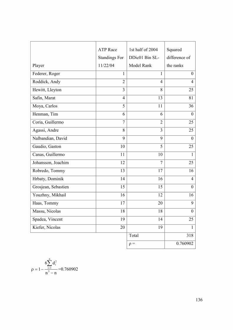
136

Player

ATP Race

Standings For

11/22/04

1st half of 2004

DDic01 Bin SL-

Model Rank

Squared

difference of

the ranks


Roddick, Andy 2 4 4




Henman, Tim 6 6 0











Haas, Tommy 17 20 9




Total 318

ρ = 0.760902

nn

d6

13

n

1i

2

i

−−=ρ∑= =0.760902

137





σ2 = 0.052632

z = 3.316696

α = 0.95


Reject H0.


between the ranks obtained by the DDic01 binary SL-model on the first half of 2004 data,

and the ATP ranks.

ija

1 for agreement and


ATP Race S

tandings

2nd half o

f 2004 DDic0

1 Bin

SL-M

odel R

ank

Roger F

ederer

Andy Roddick

Lley

ton Hew

itt

Marat S

afin

Carlo

s Moya

Tim

Henman

Guillerm

o Coria

Andre A

gassi

David Nalb

andian

Gasto

n Gaudio

Guillerm

o Canas

Joach

im Jo

hansso

n

Tommy Robred

o

Dominik Hrbaty

Sebastien

Grosjean

Mikhail Y

ouzhny

Tommy Haas

Nico

las Massu

Vince S

padea

Nico

las Kiefer


2nd half of 2004 DDic01

Bin SL-Model Rank

1 2 5 3 13 9 17 6 12 19 14 8 16 7 20 4 15 10 18 11

Roger Federer 1 1

Andy Roddick 2 2 1




Tim Henman 6 9 1 1 1 1 –1


Andre Agassi 8 6 1 1 1 1 –1 –1 –1

David Nalbandian 9 12 1 1 1 1 –1 1 –1 1

Gaston Gaudio 10 19 1 1 1 1 1 1 1 1 1

Guillermo Canas 11 14 1 1 1 1 1 1 –1 1 1 –1

Joachim Johansson 12 8 1 1 1 1 –1 –1 –1 1 –1 –1 –1

Tommy Robredo 13 16 1 1 1 1 1 1 –1 1 1 –1 1 1

Dominik Hrbaty 14 7 1 1 1 1 –1 –1 –1 1 –1 –1 –1 –1 –1


Mikhail Youzhny 16 4 1 1 –1 1 –1 –1 –1 –1 –1 –1 –1 –1 –1 –1 –1

Tommy Haas 17 15 1 1 1 1 1 1 –1 1 1 –1 1 1 –1 1 –1 1

Nicolas Massu 18 10 1 1 1 1 –1 1 –1 1 –1 –1 –1 1 –1 1 –1 1 –1

Vince Spadea 19 18 1 1 1 1 1 1 1 1 1 –1 1 1 1 1 –1 1 1 1

Nicolas Kiefer 20 11 1 1 1 1 –1 1 –1 1 –1 –1 –1 1 –1 1 –1 1 –1 1 –1

139


−=



τ =∑

∑

<

<

ji

2

ij

ji

ij

a

a

= 0.36842105




σ2 = 950

S = 70

z = 2.2710999

α = 0.95


Reject H0.


between the ranks obtained by the DDic01 binary SL-model on the second half of 2004 data,

and the ATP ranks.

140

Player

ATP Race

Standings For

11/22/04

2nd half of 2004

DDic01 Bin SL-

Model Rank

Squared

difference

of the ranks


Roddick, Andy 2 2 0


Safin, Marat 4 3 1


Henman, Tim 6 9 9


Agassi, Andre 8 6 4









Haas, Tommy 17 15 4




Total 674

ρ = 0.493233

nn

d6

13

n

1i

2

i

−−=ρ∑= = 0.493233

141





σ2 = 0.052632

z = 2.149953

α = 0.95


Reject H0.


between the ranks obtained by the DDic01 binary SL-model on the second half of 2004 data,

and the ATP ranks.

We noticed that the value of τ and ρ is less than that of the bin SL-model for the data from

the first half of the year. As with the data for the whole year, we noticed the value of τ for the

data of the second half of the year remained the same as that of the bin SL-model, but the

value of ρ decreased slightly for the data of the second half of the year. Unlike the data for

the whole year, we found that the weights of the objects were not between 0 and 1, as

required by theorem 4 to get proper probabilities. This could be because the data contains too

many zeros in it.

7.6 Real Life Application of the DD01 Binary SL-Model

We then went on to try another approach to achieve weights which yield proper probabilities.

The approach is as follows: we double the values in the data, and change the zeros to ones

(even if objects were not compared). We will call this approach the doubled data zeros

become ones binary SL-model (DD01 bin SL-model).

The cumulative number of wins for 2004 doubled, and zeros made ones thus summarised on

the next page:




and zeros made ones.

(2004)

Roger F

ederer

Andy Roddick

Lley

ton Hew

itt

Marat S

afin

Carlo

s Moya

Tim

Henman

Guillerm

o Coria

Andre A

gassi

David Nalb

andian

Gasto

n Gaudio

Guillerm

o Canas

Joach

im Jo

hansso

n

Tommy Robred

o

Dominik Hrbaty

Sebastien

Grosjean

Mikhail Y

ouzhny

Tommy Haas

Nico

las Massu

Vince S

padea

Nico

las Kiefer

Roger Federer 0 14 30 14 8 10 6 10 6 8 1 1 4 2 6 4 1 1 1 6

Andy Roddick 2 0 4 16 4 6 8 2 1 1 10 8 6 4 4 1 8 1 6 12

Lleyton Hewitt 4 4 0 4 12 8 1 2 1 8 1 6 4 1 1 1 10 2 1 1

Marat Safin 1 8 4 0 1 4 6 10 8 1 4 1 4 1 4 4 1 1 2 2

Carlos Moya 2 2 4 1 0 1 1 1 6 4 1 1 14 4 1 1 1 1 1 2

Tim Henman 4 4 1 1 1 0 6 1 1 1 4 1 4 6 1 1 1 4 4 6

Guillermo Coria 2 2 1 4 10 6 0 1 4 4 1 1 4 1 4 2 1 1 1 12

Andre Agassi 6 4 4 4 4 1 4 0 1 1 1 1 4 4 4 4 10 1 4 1


Gaston Gaudio 2 1 8 1 4 1 6 1 6 0 10 1 10 1 1 1 1 1 1 1

Guillermo Canas 1 4 1 1 1 6 1 1 4 14 0 1 2 1 1 1 12 1 1 1


Tommy Robredo 1 1 1 2 1 1 1 2 1 6 4 1 0 1 1 1 1 6 1 1

Dominik Hrbaty 4 1 1 1 2 2 1 1 1 6 1 4 1 0 2 1 1 1 1 2


Mikhail Youzhny 1 1 1 1 1 4 4 1 10 1 1 1 1 8 1 0 1 4 1 8

Tommy Haas 1 2 1 1 1 1 1 6 1 1 1 1 1 1 6 1 0 1 2 4

Nicolas Massu 1 1 1 4 4 2 1 1 1 4 1 1 1 1 1 2 1 0 4 1

Vince Spadea 1 4 1 4 1 2 1 1 1 1 1 1 1 1 1 1 4 1 0 4

Nicolas Kiefer 1 1 1 4 4 4 1 1 1 1 1 6 1 4 4 4 1 1 2 0

143

From the cumulative number of wins for 2004 doubled, and zeros made ones, the weights

and ranks obtained using the SL-model for this data was calculated as before in Mathematica

Y={{0,14,30,14,8,10,6,10,6,8,1,1,4,2,6,4,1,1,1,6},{2,0,4,16,4,

6,8,2,1,1,10,8,6,4,4,1,8,1,6,12},{4,4,0,4,12,8,1,2,1,8,1,6,4,1

,1,1,10,2,1,1},{1,8,4,0,1,4,6,10,8,1,4,1,4,1,4,4,1,1,2,2},{2,2

,4,1,0,1,1,1,6,4,1,1,14,4,1,1,1,1,1,2},{4,4,1,1,1,0,6,1,1,1,4,

1,4,6,1,1,1,4,4,6},{2,2,1,4,10,6,0,1,4,4,1,1,4,1,4,2,1,1,1,12}

,{6,4,4,4,4,1,4,0,1,1,1,1,4,4,4,4,10,1,4,1},{2,1,1,6,1,1,1,1,0

,1,8,1,1,4,1,6,1,4,8,1},{2,1,8,1,4,1,6,1,6,0,10,1,10,1,1,1,1,1

,1,1},{1,4,1,1,1,6,1,1,4,14,0,1,2,1,1,1,12,1,1,1},{1,6,1,1,1,1

,1,1,1,1,4,0,1,2,1,1,1,1,1,8},{1,1,1,2,1,1,1,2,1,6,4,1,0,1,1,1

,1,6,1,1},{4,1,1,1,2,2,1,1,1,6,1,4,1,0,2,1,1,1,1,2},{1,1,1,1,1

,1,2,1,1,1,1,1,1,6,0,6,2,1,1,1},{1,1,1,1,1,4,4,1,10,1,1,1,1,8,

1,0,1,4,1,8},{1,2,1,1,1,1,1,6,1,1,1,1,1,1,6,1,0,1,2,4},{1,1,1,

4,4,2,1,1,1,4,1,1,1,1,1,2,1,0,4,1},{1,4,1,4,1,2,1,1,1,1,1,1,1,

1,1,1,4,1,0,4},{1,1,1,4,4,4,1,1,1,1,1,6,1,4,4,4,1,1,2,0}}


{p[1]→0.872914,p[2]→0.606218,p[3]→0.464433,p[4]→0.385799,p[5]

→0.243954,p[6]→0.310318,p[7]→0.425883,p[8]→0.53486,p[9]→0.303

993,p[10]→0.286521,p[11]→0.312851,p[12]→0.293871,p[13]→0.0653

021,p[14]→0.186385,p[15]→0.175566,p[16]→0.390476,p[17]→0.1227

26,p[18]→0.29549,p[19]→0.215774,p[20]→0.1}

144


ATP Race

Standings For


2004 DD01 Bin

SL-Model

Weight

2004 DD01 Bin

SL-Model Rank





















We noted that all the weights of the objects are between zero and one, which yields proper

probabilities.

We then calculated Kendal's τ and Spearman's ρ and used them to test the association

between the DD01 binary SL-model ranks and the official ranks.

ija

1 for agreement and


ATP Race S

tandings

2004 DD01 Bin SL-M

odel

Rank

Roger F

ederer

Andy Roddick

Lley

ton Hew

itt

Marat S

afin

Carlo

s Moya

Tim

Henman

Guillerm

o Coria

Andre A

gassi

David Nalb

andian

Gasto

n Gaudio

Guillerm

o Canas

Joach

im Jo

hansso

n

Tommy Robred

o

Dominik Hrbaty

Sebastien

Grosjean

Mikhail Y

ouzhny

Tommy Haas

Nico

las Massu

Vince S

padea

Nico

las Kiefer


2004 DD01 Bin SL-

Model Rank

1 2 4 7 14 9 5 3 10 13 8 12 20 16 17 6 18 11 15 19

Roger Federer 1 1

Andy Roddick 2 2 1




Tim Henman 6 9 1 1 1 1 –1


Andre Agassi 8 3 1 1 –1 –1 –1 –1 –1


Gaston Gaudio 10 13 1 1 1 1 –1 1 1 1 1

Guillermo Canas 11 8 1 1 1 1 –1 –1 1 1 –1 –1

Joachim Johansson 12 12 1 1 1 1 –1 1 1 1 1 –1 1

Tommy Robredo 13 20 1 1 1 1 1 1 1 1 1 1 1 1

Dominik Hrbaty 14 16 1 1 1 1 1 1 1 1 1 1 1 1 –1


Mikhail Youzhny 16 6 1 1 1 –1 –1 –1 1 1 –1 –1 –1 –1 –1 –1 –1

Tommy Haas 17 18 1 1 1 1 1 1 1 1 1 1 1 1 –1 1 1 1

Nicolas Massu 18 11 1 1 1 1 –1 1 1 1 1 –1 1 –1 –1 –1 –1 1 –1

Vince Spadea 19 15 1 1 1 1 1 1 1 1 1 1 1 1 –1 –1 –1 1 –1 1

Nicolas Kiefer 20 19 1 1 1 1 1 1 1 1 1 1 1 1 –1 1 1 1 1 1 1

146

−=



τ =∑

∑

<

<

ji

2

ij

ji

ij

a

a

= 0.55789474




σ2 = 950

S = 106

z = 3.43909413

α = 0.95


Reject H0.


between the ranks obtained by the DD01 binary SL-model on the 2004 data, and the ATP

ranks.

147

Player

ATP Race

Standings For

11/22/04

2004 DD01 Bin

SL-Model Rank

Squared

difference of

the ranks


Roddick, Andy 2 2 0


Safin, Marat 4 7 9


Henman, Tim 6 9 9











Haas, Tommy 17 18 1




Total 372

ρ = 0.720301

nn

d6

13

n

1i

2

i

−−=ρ∑= = 0.720301

148




σ2 = 0.052632

z = 3.139718

α = 0.95


Reject H0.


between the ranks obtained by the DD01 binary SL-model on the 2004 data, and the ATP

ranks.

We noticed the value of τ and ρ decreased to that of the DDic01 bin SL-model. We then

proceeded to do the same analysis on the cumulative number of wins for the first half, and

then the second half of 2004 doubled, with zeros made ones.






Roger F

ederer

Andy Roddick

Lley

ton Hew

itt

Marat S

afin

Carlo

s Moya

Tim

Henman

Guillerm

o Coria

Andre A

gassi

David Nalb

andian

Gasto

n Gaudio

Guillerm

o Canas

Joach

im Jo

hansso

n

Tommy Robred

o

Dominik Hrbaty

Sebastien

Grosjean

Mikhail Y

ouzhny

Tommy Haas

Nico

las Massu

Vince S

padea

Nico

las Kiefer

Roger Federer 0 6 16 10 4 4 6 4 6 4 1 1 4 1 6 4 1 1 1 6

Andy Roddick 2 0 4 8 4 2 4 1 1 1 4 4 1 1 4 1 1 1 6 1

Lleyton Hewitt 4 1 0 1 8 4 1 1 1 4 1 1 1 1 1 1 4 1 1 1

Marat Safin 1 6 1 0 1 1 2 6 2 1 1 1 4 1 4 1 1 1 2 1

Carlos Moya 1 2 2 1 0 1 1 1 6 1 1 1 14 4 1 1 1 1 1 1

Tim Henman 4 4 1 1 1 0 2 1 1 1 4 1 4 1 1 1 1 4 4 1

Guillermo Coria 2 2 1 4 10 6 0 1 4 4 1 1 4 1 4 2 1 1 1 12

Andre Agassi 2 1 1 4 1 1 4 0 1 1 1 1 1 4 4 4 1 1 1 1


Gaston Gaudio 2 1 8 1 4 1 6 1 6 0 6 1 10 1 1 1 1 1 1 1

Guillermo Canas 1 4 1 1 1 6 1 1 1 8 0 1 2 1 1 1 4 1 1 1


Tommy Robredo 1 1 1 2 1 1 1 1 1 6 4 1 0 1 1 1 1 6 1 1

Dominik Hrbaty 1 1 1 1 2 1 1 1 1 6 1 1 1 0 2 1 1 1 1 1


Mikhail Youzhny 1 1 1 1 1 1 4 1 1 1 1 1 1 4 1 0 1 1 1 4

Tommy Haas 1 1 1 1 1 1 1 1 1 1 1 1 1 1 1 1 0 1 2 1

Nicolas Massu 1 1 1 4 1 2 1 1 1 1 1 1 1 1 1 1 1 0 1 1

Vince Spadea 1 4 1 4 1 2 1 1 1 1 1 1 1 1 1 1 4 1 0 4

Nicolas Kiefer 1 1 1 1 1 1 1 1 1 1 1 2 1 1 4 2 1 1 2 0






Roger F

ederer

Andy Roddick

Lley

ton Hew

itt

Marat S

afin

Carlo

s Moya

Tim

Henman

Guillerm

o Coria

Andre A

gassi

David Nalb

andian

Gasto

n Gaudio

Guillerm

o Canas

Joach

im Jo

hansso

n

Tommy Robred

o

Dominik Hrbaty

Sebastien

Grosjean

Mikhail Y

ouzhny

Tommy Haas

Nico

las Massu

Vince S

padea

Nico

las Kiefer

Roger Federer 0 8 14 4 4 6 1 6 1 4 1 1 1 2 1 1 1 1 1 1

Andy Roddick 1 0 1 8 1 4 4 2 1 1 6 4 6 4 1 1 8 1 1 12

Lleyton Hewitt 1 4 0 4 4 4 1 2 1 4 1 6 4 1 1 1 6 2 1 1

Marat Safin 1 2 4 0 1 4 4 4 6 1 4 1 1 1 1 4 1 1 1 2

Carlos Moya 2 1 2 1 0 1 1 1 1 4 1 1 1 1 1 1 1 1 1 2

Tim Henman 1 1 1 1 1 0 4 1 1 1 1 1 1 6 1 1 1 1 1 6

Guillermo Coria 1 1 1 1 1 1 0 1 1 1 1 1 1 1 1 1 1 1 1 1

Andre Agassi 4 4 4 1 4 1 1 0 1 1 1 1 4 1 1 1 10 1 4 1


Gaston Gaudio 1 1 1 1 1 1 1 1 1 0 4 1 1 1 1 1 1 1 1 1

Guillermo Canas 1 1 1 1 1 1 1 1 4 6 0 1 1 1 1 1 8 1 1 1


Tommy Robredo 1 1 1 1 1 1 1 2 1 1 1 1 0 1 1 1 1 1 1 1

Dominik Hrbaty 4 1 1 1 1 2 1 1 1 1 1 4 1 0 1 1 1 1 1 2


Mikhail Youzhny 1 1 1 1 1 4 1 1 10 1 1 1 1 4 1 0 1 4 1 4

Tommy Haas 1 2 1 1 1 1 1 6 1 1 1 1 1 1 6 1 0 1 1 4

Nicolas Massu 1 1 1 1 4 1 1 1 1 4 1 1 1 1 1 2 1 0 4 1

Vince Spadea 1 1 1 1 1 1 1 1 1 1 1 1 1 1 1 1 1 1 0 1

Nicolas Kiefer 1 1 1 4 4 4 1 1 1 1 1 4 1 4 1 2 1 1 1 0

151

The weights and ranks obtained using the SL-model on cumulative number of wins for the

first half, and then the second half of 2004 doubled, both with zeros made ones, was

calculated as before in Mathematica.

Y={{0,6,16,10,4,4,6,4,6,4,1,1,4,1,6,4,1,1,1,6},{2,0,4,8,4,2,4,1,1,1,4,4,1,1,4,1,1,1,6,1},{4,1,0,1,8,4,1,1,1,4,1,1,1,1,1,1,4,1,1,1},{1,6,1,0,1,1,2,6,2,1,1,1,4,1,4,1,1,1,2,1},{1,2,2,1,0,1,1,1,6,1,1,1,14,4,1,1,1,1,1,1},{4,4,1,1,1,0,2,1,1,1,4,1,4,1,1,1,1,4,4,1},{2,2,1,4,10,6,0,1,4,4,1,1,4,1,4,2,1,1,1,12},{2,1,1,4,1,1,4,0,1,1,1,1,1,4,4,4,1,1,1,1},{2,1,1,6,1,1,1,1,0,1,6,1,1,4,1,1,1,1,4,1},{2,1,8,1,4,1,6,1,6,0,6,1,10,1,1,1,1,1,1,1},{1,4,1,1,1,6,1,1,1,8,0,1,2,1,1,1,4,1,1,1},{1,1,1,1,1,1,1,1,1,1,1,0,1,1,1,1,1,1,1,8},{1,1,1,2,1,1,1,1,1,6,4,1,0,1,1,1,1,6,1,1},{1,1,1,1,2,1,1,1,1,6,1,1,1,0,2,1,1,1,1,1},{1,1,1,1,1,1,2,1,1,1,1,1,1,6,0,6,1,1,1,1},{1,1,1,1,1,1,4,1,1,1,1,1,1,4,1,0,1,1,1,4},{1,1,1,1,1,1,1,1,1,1,1,1,1,1,1,1,0,1,2,1},{1,1,1,4,1,2,1,1,1,1,1,1,1,1,1,1,1,0,1,1},{1,4,1,4,1,2,1,1,1,1,1,1,1,1,1,1,4,1,0,4},{1,1,1,1,1,1,1,1,1,1,1,2,1,1,4,2,1,1,2,0}}


{p[1]→0.830376,p[2]→0.499501,p[3]→0.378744,p[4]→0.257235,p[5]

→0.336571,p[6]→0.418081,p[7]→0.573793,p[8]→0.494131,p[9]→0.36

8851,p[10]→0.44904,p[11]→0.377154,p[12]→0.395556,p[13]→0.1543

36,p[14]→0.219685,p[15]→0.237944,p[16]→0.307766,p[17]→0.21906

8,p[18]→0.272986,p[19]→0.341943,p[20]→0.1}

152

Y={{0,8,14,4,4,6,1,6,1,4,1,1,1,2,1,1,1,1,1,1},{1,0,1,8,1,4,4,2,1,1,6,4,6,4,1,1,8,1,1,12},{1,4,0,4,4,4,1,2,1,4,1,6,4,1,1,1,6,2,1,1},{1,2,4,0,1,4,4,4,6,1,4,1,1,1,1,4,1,1,1,2},{2,1,2,1,0,1,1,1,1,4,1,1,1,1,1,1,1,1,1,2},{1,1,1,1,1,0,4,1,1,1,1,1,1,6,1,1,1,1,1,6},{1,1,1,1,1,1,0,1,1,1,1,1,1,1,1,1,1,1,1,1},{4,4,4,1,4,1,1,0,1,1,1,1,4,1,1,1,10,1,4,1},{1,1,1,1,1,1,1,1,0,1,2,1,1,1,1,6,1,4,4,1},{1,1,1,1,1,1,1,1,1,0,4,1,1,1,1,1,1,1,1,1},{1,1,1,1,1,1,1,1,4,6,0,1,1,1,1,1,8,1,1,1},{1,6,1,1,1,1,1,1,1,1,4,0,1,2,1,1,1,1,1,1},{1,1,1,1,1,1,1,2,1,1,1,1,0,1,1,1,1,1,1,1},{4,1,1,1,1,2,1,1,1,1,1,4,1,0,1,1,1,1,1,2},{1,1,1,1,1,1,1,1,1,1,1,1,1,1,0,1,2,1,1,1},{1,1,1,1,1,4,1,1,10,1,1,1,1,4,1,0,1,4,1,4},{1,2,1,1,1,1,1,6,1,1,1,1,1,1,6,1,0,1,1,4},{1,1,1,1,4,1,1,1,1,4,1,1,1,1,1,2,1,0,4,1},{1,1,1,1,1,1,1,1,1,1,1,1,1,1,1,1,1,1,0,1},{1,1,1,4,4,4,1,1,1,1,1,4,1,4,1,2,1,1,1,0}}

y[i_,j_]:=Extract[Y,{i,j}]

l[i_,j_]:=y[i,j]/(p[i]+1-p[j])

r[i_,j_]:=l[j,i]

s[i_,j_]:=l[i,j]-r[i,j]

e[i_]:=Sum[s[i,j],{j,1,20}]


{p[1]→0.874381,p[2]→0.767283,p[3]→0.655512,p[4]→0.644122,p[5]

→0.376358,p[6]→0.400856,p[7]→0.332007,p[8]→0.645403,p[9]→0.45

1899,p[10]→0.281825,p[11]→0.473016,p[12]→0.456345,p[13]→0.342

818,p[14]→0.408891,p[15]→0.395257,p[16]→0.63159,p[17]→0.35717

7,p[18]→0.531138,p[19]→0.326858,p[20]→0.4}

153


ATP Race

Standings

For


1st half of

2004 DD01

Bin SL-Model

Weight

1st half of

2004

DD01 Bin

SL-Model

Rank

2nd half of

2004 DD01

Bin SL-

Model

Weight

2nd half of

2004 DD01

Bin SL-

Model Rank


2 Roddick, Andy USA 0.499501 3 0.767283 2


4 Safin, Marat RUS 0.257235 15 0.644122 5

5 Moya, Carlos ESP 0.336571 12 0.376358 15

6 Henman, Tim GBR 0.418081 6 0.400856 12

7 Coria, Guillermo ARG 0.573793 2 0.332007 18

8 Agassi, Andre USA 0.494131 4 0.645403 4


10 Gaudio, Gaston ARG 0.44904 5 0.281825 20





15 Grosjean, Sebastien FRA 0.237944 16 0.395257 14


17 Haas, Tommy GER 0.219068 18 0.357177 16


19 Spadea, Vincent USA 0.341943 11 0.326858 19


Kendal's τ and Spearman's ρ and the tests for association between the DD01 bin SL-model

ranks and the official ranks follow as:

ija

1 for agreement and


ATP Race S

tandings

1st h

alf of 2

004 DD01

Bin SL-M

odel R

ank

Roger F

ederer

Andy Roddick

Lley

ton Hew

itt

Marat S

afin

Carlo

s Moya

Tim

Henman

Guillerm

o Coria

Andre A

gassi

David Nalb

andian

Gasto

n Gaudio

Guillerm

o Canas

Joach

im Jo

hansso

n

Tommy Robred

o

Dominik Hrbaty

Sebastien

Grosjean

Mikhail Y

ouzhny

Tommy Haas

Nico

las Massu

Vince S

padea

Nico

las Kiefer


1st half of 2004 DD01 Bin

SL-Model Rank

1 4 8 13 11 6 2 3 9 5 10 7 17 16 15 12 20 18 14 19

Roger Federer 1 1

Andy Roddick 2 4 1




Tim Henman 6 6 1 1 –1 –1 –1

Guillermo Coria 7 2 1 –1 –1 –1 –1 –1

Andre Agassi 8 3 1 –1 –1 –1 –1 –1 1


Gaston Gaudio 10 5 1 1 –1 –1 –1 –1 1 1 –1

Guillermo Canas 11 10 1 1 1 –1 –1 1 1 1 1 1

Joachim Johansson 12 7 1 1 –1 –1 –1 1 1 1 –1 1 –1

Tommy Robredo 13 17 1 1 1 1 1 1 1 1 1 1 1 1

Dominik Hrbaty 14 16 1 1 1 1 1 1 1 1 1 1 1 1 –1


Mikhail Youzhny 16 12 1 1 1 –1 1 1 1 1 1 1 1 1 –1 –1 –1

Tommy Haas 17 20 1 1 1 1 1 1 1 1 1 1 1 1 1 1 1 1

Nicolas Massu 18 18 1 1 1 1 1 1 1 1 1 1 1 1 1 1 1 1 –1

Vince Spadea 19 14 1 1 1 1 1 1 1 1 1 1 1 1 –1 –1 –1 1 –1 –1

Nicolas Kiefer 20 19 1 1 1 1 1 1 1 1 1 1 1 1 1 1 1 1 –1 1 1

155


−=



τ =∑

∑

<

<

ji

2

ij

ji

ij

a

a

= 0.48421053



σ2 = 950

S = 92

z = 2.98487415

α = 0.95


Reject H0.


between the ranks obtained by the DD01 binary SL-model on the first half of 2004 data, and

the ATP ranks.

156

Player

ATP Race

Standings For

11/22/04

1st half of 2004

DD01 Bin SL-

Model Rank

Squared

difference of

the ranks


Roddick, Andy 2 3 1




Henman, Tim 6 6 0











Haas, Tommy 17 18 1




Total 428

ρ = 0.678195

nn

d6

13

n

1i

2

i

−−=ρ∑= =0.678195

157





σ2 = 0.052632

z = 2.956186

α = 0.95


Reject H0.


between the ranks obtained by the DD01 binary SL-model on the first half of 2004 data, and

the ATP ranks.

ija

1 for agreement and


ATP Race S

tandings

2nd half o

f 2004 DD01

Bin SL-M

odel R

ank

Roger F

ederer

Andy Roddick

Lley

ton Hew

itt

Marat S

afin

Carlo

s Moya

Tim

Henman

Guillerm

o Coria

Andre A

gassi

David Nalb

andian

Gasto

n Gaudio

Guillerm

o Canas

Joach

im Jo

hansso

n

Tommy Robred

o

Dominik Hrbaty

Sebastien

Grosjean

Mikhail Y

ouzhny

Tommy Haas

Nico

las Massu

Vince S

padea

Nico

las Kiefer


2nd half of 2004 DD01 Bin

SL-Model Rank

1 2 3 5 15 12 18 4 10 20 8 9 17 11 14 6 16 7 19 13

Roger Federer 1 1

Andy Roddick 2 2 1




Tim Henman 6 12 1 1 1 1 –1


Andre Agassi 8 4 1 1 1 –1 –1 –1 –1

David Nalbandian 9 10 1 1 1 1 –1 –1 –1 1

Gaston Gaudio 10 20 1 1 1 1 1 1 1 1 1

Guillermo Canas 11 8 1 1 1 1 –1 –1 –1 1 –1 –1

Joachim Johansson 12 9 1 1 1 1 –1 –1 –1 1 –1 –1 1

Tommy Robredo 13 17 1 1 1 1 1 1 –1 1 1 –1 1 1

Dominik Hrbaty 14 11 1 1 1 1 –1 –1 –1 1 1 –1 1 1 –1

Sebastien Grosjean 15 14 1 1 1 1 –1 1 –1 1 1 –1 1 1 –1 1

Mikhail Youzhny 16 6 1 1 1 1 –1 –1 –1 1 –1 –1 –1 –1 –1 –1 –1

Tommy Haas 17 16 1 1 1 1 1 1 –1 1 1 –1 1 1 –1 1 1 1

Nicolas Massu 18 7 1 1 1 1 –1 –1 –1 1 –1 –1 –1 –1 –1 –1 –1 1 –1

Vince Spadea 19 19 1 1 1 1 1 1 1 1 1 –1 1 1 1 1 1 1 1 1

Nicolas Kiefer 20 13 1 1 1 1 –1 1 –1 1 1 –1 1 1 –1 1 –1 1 –1 1 –1

159


−=



τ =∑

∑

<

<

ji

2

ij

ji

ij

a

a

= 0.35789474




σ2 = 950

S = 68

z = 2.20621133

α = 0.95


Reject H0.


between the ranks obtained by the DD01 binary SL-model on the second half of 2004 data,

and the ATP ranks.

160

Player

ATP Race

Standings For

11/22/04

2nd half of 2004

DD01 Bin SL-

Model Rank

Squared

difference of

the ranks


Roddick, Andy 2 2 0


Safin, Marat 4 5 1


Henman, Tim 6 12 36











Haas, Tommy 17 16 1




Total 690

ρ = 0.481203

nn

d6

13

n

1i

2

i

−−=ρ∑= = 0.481203

161





σ2 = 0.052632

z = 2.097515

α = 0.95


Reject H0.


between the ranks obtained by the DD01 binary SL-model on the second half of 2004 data,

and the ATP ranks.

As with the data for the whole year, we notice that the value of τ and ρ is less than that of the

DDic01 bin SL-model for the data from the first half and the data from second half of the

year. Also, we again found that the weights of the objects were all between 0 and 1, as

required by theorem 4 to get proper probabilities.

7.7 Comparison to other models

We noted that the official rankings was also influenced by when the top twenty players

played against other players not in the top twenty, which was not accounted for in our

analysis. Another reason why our measures of association are not higher, is due to the

method in which the official ranks are calculated which include letting some tournaments e.g.

grand slams have higher influence on scores than other tournaments, choosing best 3 games

from a tournament etc. We thus decided to compare the outcomes of the data for the whole

162

year using the general SL-model, the binary SL-model, the DDic01 binary SL-model and the

DD01 binary SL-model with other models for paired comparisons. The following ranks and

weights using other paired comparisons models were found:

Binomial Poisson B

Binomial Poisson

ML

ATP Race

Standings

For

11/22/04 Player Weights Ranks Weights Ranks

1 Federer, Roger 26.32614266 1 3175.965753 1

2 Roddick, Andy 19.43864486 3 2364.231223 3

3 Hewitt, Lleyton 17.70928622 7 2241.683929 4

4 Safin, Marat 17.90373436 5 2160.475201 5

5 Moya, Carlos 14.97394555 10 1933.287714 10

6 Henman, Tim 16.3442535 8 2002.383475 8

7 Coria, Guillermo 18.26369708 4 2117.816824 6

8 Agassi, Andre 22.45360208 2 2522.044821 2

9 Nalbandian, David 16.1078778 9 1992.317874 9

10 Gaudio, Gaston 14.53347682 12 1831.445255 13

11 Canas, Guillermo 14.91253433 11 1895.537385 11

12 Johansson, Joachim 14.32924027 15 1838.86228 12

13 Robredo, Tommy 12.77321182 19 1604.142581 18

14 Hrbaty, Dominik 13.21575788 18 1563.963008 20

15 Grosjean, Sebastien 14.42765157 13 1762.81286 15

16 Youzhny, Mikhail 17.83837001 6 2043.757559 7

17 Haas, Tommy 14.34440777 14 1693.427461 16

18 Massu, Nicolas 14.05871733 16 1796.641759 14

19 Spadea, Vincent 12.19231423 20 1692.152007 17

20 Kiefer, Nicolas 13.26149865 17 1583.387812 19

163

Bradley-Terry

ATP Race

Standings

For

11/22/04 Player Weights Ranks

1 Federer, Roger 0.079728732 1

2 Roddick, Andy 0.059792187 3

3 Hewitt, Lleyton 0.056277387 4

4 Safin, Marat 0.054251129 5

5 Moya, Carlos 0.048648297 10

6 Henman, Tim 0.05012986 9

7 Coria, Guillermo 0.05308978 6

8 Agassi, Andre 0.063616728 2

9 Nalbandian, David 0.05035668 8

10 Gaudio, Gaston 0.046013062 12

11 Canas, Guillermo 0.047542589 11

12 Johansson, Joachim 0.045557702 13

13 Robredo, Tommy 0.040334221 18

14 Hrbaty, Dominik 0.039087149 20

15 Grosjean, Sebastien 0.044467638 15

16 Youzhny, Mikhail 0.051170951 7

17 Haas, Tommy 0.042956224 16

18 Massu, Nicolas 0.045112652 14

19 Spadea, Vincent 0.042319623 17

20 Kiefer, Nicolas 0.039547409 19

164

Poisson PoissonApprox

ATP Race

Standings

For 11/22/04

Player

Weights

Ranks

Weights

Ranks

1 Federer, Roger 5.16015047 1 2.970883013 1

2 Roddick, Andy 3.972404548 3 2.150868715 3

3 Hewitt, Lleyton 3.764006293 4 2.019767845 5

4 Safin, Marat 3.392777991 7 1.505072794 14

5 Moya, Carlos 3.024030193 11 1.65733358 11

6 Henman, Tim 3.003035721 12 1.619656812 12

7 Coria, Guillermo 3.737974584 6 2.016408647 6

8 Agassi, Andre 4.432616537 2 2.225986608 2

9 Nalbandian, David 3.27269897 8 1.800994954 9

10 Gaudio, Gaston 3.171682442 9 1.873489182 7

11 Canas, Guillermo 3.13945052 10 1.854520573 8

12 Johansson, Joachim 2.561499031 17 1.345287155 16

13 Robredo, Tommy 2.650759879 16 1.325780588 17

14 Hrbaty, Dominik 2.514576809 18 1.37174803 15

15 Grosjean, Sebastien 2.877863631 14 1.507239151 13

16 Youzhny, Mikhail 3.755308219 5 2.058324339 4

17 Haas, Tommy 2.717192249 15 1.189370168 18

18 Massu, Nicolas 2.959635214 13 1.669726009 10

19 Spadea, Vincent 2.009889636 20 1.127847091 19

20 Kiefer, Nicolas 2.13349056 19 0.970583865 20

165

RowSum

ATP Race

Standings

For

11/22/04 Player Weights Ranks

1 Federer, Roger 192 1

2 Roddick, Andy 150 2

3 Hewitt, Lleyton 96 3

4 Safin, Marat 90 4

5 Moya, Carlos 57 10

6 Henman, Tim 63 9

7 Coria, Guillermo 81 6

8 Agassi, Andre 84 5

9 Nalbandian, David 57 12

10 Gaudio, Gaston 69 7

11 Canas, Guillermo 63 8

12 Johansson, Joachim 30 16

13 Robredo, Tommy 30 18

14 Hrbaty, Dominik 33 14

15 Grosjean, Sebastien 24 20

16 Youzhny, Mikhail 57 11

17 Haas, Tommy 30 15

18 Massu, Nicolas 30 17

19 Spadea, Vincent 27 19

20 Kiefer, Nicolas 48 13

166

The ranks obtained for the various models are summarised below:

ATP Player

General S

L-M

odel

Bin SL-M

odel

DDic0

1 Bin SL-M

odel

DD01 Bin SL-M

odel

Binomial P

oisso

n B

Binomial P

oisso

n M

L

Brad

ley

Poisso

n

Poisso

n Approx

Row Sum

1 Federer, Roger 1 1 1 1 1 1 1 1 1 1

2 Roddick, Andy 3 2 2 2 3 3 3 3 3 2

3 Hewitt, Lleyton 4 4 4 4 7 4 4 4 5 3

4 Safin, Marat 5 6 7 7 5 5 5 7 14 4

5 Moya, Carlos 10 12 14 14 10 10 10 11 11 10

6 Henman, Tim 9 8 8 9 8 8 9 12 12 9

7 Coria, Guillermo 6 5 5 5 4 6 6 6 6 6

8 Agassi, Andre 2 3 3 3 2 2 2 2 2 5

9 Nalbandian, David 8 9 9 10 9 9 8 8 9 12

10 Gaudio, Gaston 12 10 10 13 12 13 12 9 7 7

11 Canas, Guillermo 11 11 11 8 11 11 11 10 8 8

12 Johansson, Joachim 14 13 12 12 15 12 13 17 16 16

13 Robredo, Tommy 18 20 19 20 19 18 18 16 17 18

14 Hrbaty, Dominik 20 15 15 16 18 20 20 18 15 14

15 Grosjean, Sebastien 15 19 16 17 13 15 15 14 13 20

16 Youzhny, Mikhail 7 7 6 6 6 7 7 5 4 11

17 Haas, Tommy 16 17 20 18 14 16 16 15 18 15

18 Massu, Nicolas 13 14 13 11 16 14 14 13 10 17

19 Spadea, Vincent 17 16 17 15 20 17 17 20 19 19

20 Kiefer, Nicolas 19 18 18 19 17 19 19 19 20 13

Kendal's τ, Spearman's ρ and the tests for association between the various ranks follow.

7.7.1 General SL-Model vs Binary SL-Model

1 for agreement and


General S

L-M

odel

Bin SL-M

odel

Roger F

ederer

Andy Roddick

Lley

ton Hew

itt

Marat S

afin

Carlo

s Moya

Tim

Henman

Guillerm

o Coria

Andre A

gassi

David Nalb

andian

Gasto

n Gaudio

Guillerm

o Canas

Joach

im Jo

hansso

n

Tommy Robred

o

Dominik Hrbaty

Sebastien

Grosjean

Mikhail Y

ouzhny

Tommy Haas

Nico

las Massu

Vince S

padea

Nico

las Kiefer

General SL-Model 1 3 4 5 10 9 6 2 8 12 11 14 18 20 15 7 16 13 17 19

Bin SL-Model 1 2 4 6 12 8 5 3 9 10 11 13 20 15 19 7 17 14 16 18

Roger Federer 1 1

Andy Roddick 3 2 1




Tim Henman 9 8 1 1 1 1 1

Guillermo Coria 6 5 1 1 1 –1 1 1

Andre Agassi 2 3 1 –1 1 1 1 1 1

David Nalbandian 8 9 1 1 1 1 1 –1 1 1

Gaston Gaudio 12 10 1 1 1 1 –1 1 1 1 1

Guillermo Canas 11 11 1 1 1 1 –1 1 1 1 1 –1


Tommy Robredo 18 20 1 1 1 1 1 1 1 1 1 1 1 1

Dominik Hrbaty 20 15 1 1 1 1 1 1 1 1 1 1 1 1 –1

Sebastien Grosjean 15 19 1 1 1 1 1 1 1 1 1 1 1 1 1 –1

Mikhail Youzhny 7 7 1 1 1 1 1 1 1 1 1 1 1 1 1 1 1

Tommy Haas 16 17 1 1 1 1 1 1 1 1 1 1 1 1 1 –1 –1 1

Nicolas Massu 13 14 1 1 1 1 1 1 1 1 1 1 1 –1 1 1 1 1 1

Vince Spadea 17 16 1 1 1 1 1 1 1 1 1 1 1 1 1 –1 –1 1 –1 1

Nicolas Kiefer 19 18 1 1 1 1 1 1 1 1 1 1 1 1 –1 –1 –1 1 1 1 1

168

−=



τ =∑

∑

<

<

ji

2

ij

ji

ij

a

a

= 0.82105263




σ2 = 950

S = 156

z = 5.06130834

α = 0.95


Reject H0.


between the ranks obtained by the general SL-model and the ranks obtained by the binary SL-

model.

169

Player

General

SL-

Model

Bin

SL-

Model

Squared

difference of

the ranks


Roddick, Andy 3 2 1


Safin, Marat 5 6 1


Henman, Tim 9 8 1


Agassi, Andre 2 3 1









Haas, Tommy 16 17 1




Total 64

ρ = 0.95188

170

nn

d6

13

n

1i

2

i

−−=ρ∑= = 0.95188




σ2 = 0.052632

z = 4.149147

α = 0.95


Reject H0.


between the ranks obtained by the general SL-model and the ranks obtained by the binary SL-

model.

7.7.2 General SL-Model vs DDic01 Binary SL-Model

1 for agreement and


General S

L-M

odel

DDic0

1 Bin SL-M

odel

Roger F

ederer

Andy Roddick

Lley

ton Hew

itt

Marat S

afin

Carlo

s Moya

Tim

Henman

Guillerm

o Coria

Andre A

gassi

David Nalb

andian

Gasto

n Gaudio

Guillerm

o Canas

Joach

im Jo

hansso

n

Tommy Robred

o

Dominik Hrbaty

Sebastien

Grosjean

Mikhail Y

ouzhny

Tommy Haas

Nico

las Massu

Vince S

padea

Nico

las Kiefer

General SL-Model 1 3 4 5 10 9 6 2 8 12 11 14 18 20 15 7 16 13 17 19

DDic01 Bin SL-Model 1 2 4 7 14 8 5 3 9 10 11 12 19 15 16 6 20 13 17 18

Roger Federer 1 1

Andy Roddick 3 2 1




Tim Henman 9 8 1 1 1 1 1


Andre Agassi 2 3 1 –1 1 1 1 1 1


Gaston Gaudio 12 10 1 1 1 1 –1 1 1 1 1

Guillermo Canas 11 11 1 1 1 1 –1 1 1 1 1 –1


Tommy Robredo 18 19 1 1 1 1 1 1 1 1 1 1 1 1

Dominik Hrbaty 20 15 1 1 1 1 1 1 1 1 1 1 1 1 –1


Mikhail Youzhny 7 6 1 1 1 –1 1 1 1 1 1 1 1 1 1 1 1

Tommy Haas 16 20 1 1 1 1 1 1 1 1 1 1 1 1 –1 –1 1 1

Nicolas Massu 13 13 1 1 1 1 –1 1 1 1 1 1 1 –1 1 1 1 1 1

Vince Spadea 17 17 1 1 1 1 1 1 1 1 1 1 1 1 1 –1 1 1 –1 1

Nicolas Kiefer 19 18 1 1 1 1 1 1 1 1 1 1 1 1 –1 –1 1 1 –1 1 1

172

−=



τ =∑

∑

<

<

ji

2

ij

ji

ij

a

a

= 0.8




σ2 = 950

S = 152

z = 4.9315312

α = 0.95


Reject H0.


between the ranks obtained by the general SL-model and the ranks obtained by the DDic01

binary SL-model.

173

Player

General

SL-

Model

DDic01

Bin SL-

Model

Squared

difference

of the ranks


Roddick, Andy 3 2 1


Safin, Marat 5 7 4


Henman, Tim 9 8 1


Agassi, Andre 2 3 1













Total 78

ρ = 0.941353

174

nn

d6

13

n

1i

2

i

−−=ρ∑= = 0.941353




σ2 = 0.052632

z = 4.103264

α = 0.95


Reject H0.


between the ranks obtained by the general SL-model and the ranks obtained by the DDic01

binary SL-model.

7.7.3 General SL-Model vs DD01 Binary SL-Model

1 for agreement and


General S

L-M

odel

DD01 Bin SL-M

odel

Roger F

ederer

Andy Roddick

Lley

ton Hew

itt

Marat S

afin

Carlo

s Moya

Tim

Henman

Guillerm

o Coria

Andre A

gassi

David Nalb

andian

Gasto

n Gaudio

Guillerm

o Canas

Joach

im Jo

hansso

n

Tommy Robred

o

Dominik Hrbaty

Sebastien

Grosjean

Mikhail Y

ouzhny

Tommy Haas

Nico

las Massu

Vince S

padea

Nico

las Kiefer

General SL-Model 1 3 4 5 10 9 6 2 8 12 11 14 18 20 15 7 16 13 17 19

DD01 Bin SL-Model 1 2 4 7 14 9 5 3 10 13 8 12 20 16 17 6 18 11 15 19

Roger Federer 1 1

Andy Roddick 3 2 1




Tim Henman 9 9 1 1 1 1 1


Andre Agassi 2 3 1 –1 1 1 1 1 1


Gaston Gaudio 12 13 1 1 1 1 –1 1 1 1 1

Guillermo Canas 11 8 1 1 1 1 –1 –1 1 1 –1 1


Tommy Robredo 18 20 1 1 1 1 1 1 1 1 1 1 1 1

Dominik Hrbaty 20 16 1 1 1 1 1 1 1 1 1 1 1 1 –1


Mikhail Youzhny 7 6 1 1 1 –1 1 1 1 1 1 1 1 1 1 1 1

Tommy Haas 16 18 1 1 1 1 1 1 1 1 1 1 1 1 1 –1 1 1

Nicolas Massu 13 11 1 1 1 1 –1 1 1 1 1 –1 1 1 1 1 1 1 1

Vince Spadea 17 15 1 1 1 1 1 1 1 1 1 1 1 1 1 1 –1 1 –1 1

Nicolas Kiefer 19 19 1 1 1 1 1 1 1 1 1 1 1 1 –1 –1 1 1 1 1 1

176

−=



τ =∑

∑

<

<

ji

2

ij

ji

ij

a

a

= 0.8




σ2 = 950

S = 152

z = 4.9315312

α = 0.95


Reject H0.


between the ranks obtained by the general SL-model and the ranks obtained by the DD01

binary SL-model.

177

Player

General

SL-

Model

DD01

Bin SL-

Model

Squared

difference

of the ranks


Roddick, Andy 3 2 1


Safin, Marat 5 7 4


Henman, Tim 9 9 0


Agassi, Andre 2 3 1









Haas, Tommy 16 18 4




Total 78

ρ = 0.941353

178

nn

d6

13

n

1i

2

i

−−=ρ∑= = 0.941353




σ2 = 0.052632

z = 4.103264

α = 0.95


Reject H0.


between the ranks obtained by the general SL-model and the ranks obtained by the DD01

binary SL-model.

7.7.4 General SL-Model vs Binomial Poisson Model (Bayesian Solution)

1 for agreement and


General S

L-M

odel

Binomial P

oisso

n B

Roger F

ederer

Andy Roddick

Lley

ton Hew

itt

Marat S

afin

Carlo

s Moya

Tim

Henman

Guillerm

o Coria

Andre A

gassi

David Nalb

andian

Gasto

n Gaudio

Guillerm

o Canas

Joach

im Jo

hansso

n

Tommy Robred

o

Dominik Hrbaty

Sebastien

Grosjean

Mikhail Y

ouzhny

Tommy Haas

Nico

las Massu

Vince S

padea

Nico

las Kiefer

General SL-Model 1 3 4 5 10 9 6 2 8 12 11 14 18 20 15 7 16 13 17 19

Binomial Poisson B 1 3 7 5 10 8 4 2 9 12 11 15 19 18 13 6 14 16 20 17

Roger Federer 1 1

Andy Roddick 3 3 1




Tim Henman 9 8 1 1 1 1 1

Guillermo Coria 6 4 1 1 –1 –1 1 1

Andre Agassi 2 2 1 1 1 1 1 1 1


Gaston Gaudio 12 12 1 1 1 1 1 1 1 1 1

Guillermo Canas 11 11 1 1 1 1 1 1 1 1 1 1


Tommy Robredo 18 19 1 1 1 1 1 1 1 1 1 1 1 1

Dominik Hrbaty 20 18 1 1 1 1 1 1 1 1 1 1 1 1 –1

Sebastien Grosjean 15 13 1 1 1 1 1 1 1 1 1 1 1 –1 1 1

Mikhail Youzhny 7 6 1 1 –1 1 1 1 1 1 1 1 1 1 1 1 1

Tommy Haas 16 14 1 1 1 1 1 1 1 1 1 1 1 –1 1 1 1 1

Nicolas Massu 13 16 1 1 1 1 1 1 1 1 1 1 1 –1 1 1 –1 1 –1

Vince Spadea 17 20 1 1 1 1 1 1 1 1 1 1 1 1 –1 –1 1 1 1 1

Nicolas Kiefer 19 17 1 1 1 1 1 1 1 1 1 1 1 1 –1 1 1 1 1 1 –1

180

−=



τ =∑

∑

<

<

ji

2

ij

ji

ij

a

a

= 0.84210526




σ2 = 950

S = 160

z = 5.19108548

α = 0.95


Reject H0.


between the ranks obtained by the general SL-model and the ranks obtained by the bayesian

binomial poisson model.

181

Player

General

SL-

Model

Binomial

Poisson

B

Squared

difference

of the ranks


Roddick, Andy 3 3 0


Safin, Marat 5 5 0


Henman, Tim 9 8 1


Agassi, Andre 2 2 0









Haas, Tommy 16 14 4




Total 52

ρ = 0.960902

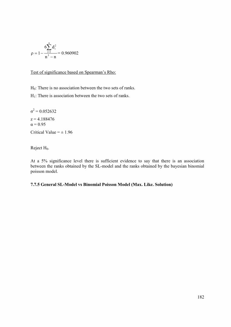
182

nn

d6

13

n

1i

2

i

−−=ρ∑= = 0.960902




σ2 = 0.052632

z = 4.188476

α = 0.95


Reject H0.


between the ranks obtained by the SL-model and the ranks obtained by the bayesian binomial

poisson model.

7.7.5 General SL-Model vs Binomial Poisson Model (Max. Like. Solution)

1 for agreement and


General S

L-M

odel

Binomial P

oisso

n M

L

Roger F

ederer

Andy Roddick

Lley

ton Hew

itt

Marat S

afin

Carlo

s Moya

Tim

Henman

Guillerm

o Coria

Andre A

gassi

David Nalb

andian

Gasto

n Gaudio

Guillerm

o Canas

Joach

im Jo

hansso

n

Tommy Robred

o

Dominik Hrbaty

Sebastien

Grosjean

Mikhail Y

ouzhny

Tommy Haas

Nico

las Massu

Vince S

padea

Nico

las Kiefer

General SL-Model 1 3 4 5 10 9 6 2 8 12 11 14 18 20 15 7 16 13 17 19

Binomial Poisson ML 1 3 4 5 10 8 6 2 9 13 11 12 18 20 15 7 16 14 17 19

Roger Federer 1 1

Andy Roddick 3 3 1




Tim Henman 9 8 1 1 1 1 1


Andre Agassi 2 2 1 1 1 1 1 1 1


Gaston Gaudio 12 13 1 1 1 1 1 1 1 1 1

Guillermo Canas 11 11 1 1 1 1 1 1 1 1 1 1

Joachim Johansson 14 12 1 1 1 1 1 1 1 1 1 –1 1

Tommy Robredo 18 18 1 1 1 1 1 1 1 1 1 1 1 1

Dominik Hrbaty 20 20 1 1 1 1 1 1 1 1 1 1 1 1 1


Mikhail Youzhny 7 7 1 1 1 1 1 1 1 1 1 1 1 1 1 1 1

Tommy Haas 16 16 1 1 1 1 1 1 1 1 1 1 1 1 1 1 1 1

Nicolas Massu 13 14 1 1 1 1 1 1 1 1 1 1 1 –1 1 1 1 1 1

Vince Spadea 17 17 1 1 1 1 1 1 1 1 1 1 1 1 1 1 1 1 1 1

Nicolas Kiefer 19 19 1 1 1 1 1 1 1 1 1 1 1 1 1 1 1 1 1 1 1

184

−=



τ =∑

∑

<

<

ji

2

ij

ji

ij

a

a

= 0.96842105




σ2 = 950

S = 184

z = 5.9697483

α = 0.95


Reject H0.


between the ranks obtained by the general SL-model and the ranks obtained by the maximum

likelihood binomial poisson model.

185

Player

General

SL-

Model

Binomial

Poisson

ML

Squared

difference

of the ranks


Roddick, Andy 3 3 0


Safin, Marat 5 5 0


Henman, Tim 9 8 1


Agassi, Andre 2 2 0









Haas, Tommy 16 16 0




Total 8

ρ = 0.993985

186

nn

d6

13

n

1i

2

i

−−=ρ∑= = 0.993985




σ2 = 0.052632

z = 4.33268

α = 0.95


Reject H0.


between the ranks obtained by the general SL-model and the ranks obtained by the maximum


7.7.6 General SL-Model vs Bradley-Terry Model

1 for agreement and


General S

L-M

odel

Brad

ley-Terry

Roger F

ederer

Andy Roddick

Lley

ton Hew

itt

Marat S

afin

Carlo

s Moya

Tim

Henman

Guillerm

o Coria

Andre A

gassi

David Nalb

andian

Gasto

n Gaudio

Guillerm

o Canas

Joach

im Jo

hansso

n

Tommy Robred

o

Dominik Hrbaty

Sebastien

Grosjean

Mikhail Y

ouzhny

Tommy Haas

Nico

las Massu

Vince S

padea

Nico

las Kiefer

General SL-Model 1 3 4 5 10 9 6 2 8 12 11 14 18 20 15 7 16 13 17 19

Bradley-Terry 1 3 4 5 10 9 6 2 8 12 11 13 18 20 15 7 16 14 17 19

Roger Federer 1 1

Andy Roddick 3 3 1




Tim Henman 9 9 1 1 1 1 1


Andre Agassi 2 2 1 1 1 1 1 1 1

David Nalbandian 8 8 1 1 1 1 1 1 1 1

Gaston Gaudio 12 12 1 1 1 1 1 1 1 1 1

Guillermo Canas 11 11 1 1 1 1 1 1 1 1 1 1


Tommy Robredo 18 18 1 1 1 1 1 1 1 1 1 1 1 1

Dominik Hrbaty 20 20 1 1 1 1 1 1 1 1 1 1 1 1 1


Mikhail Youzhny 7 7 1 1 1 1 1 1 1 1 1 1 1 1 1 1 1

Tommy Haas 16 16 1 1 1 1 1 1 1 1 1 1 1 1 1 1 1 1

Nicolas Massu 13 14 1 1 1 1 1 1 1 1 1 1 1 –1 1 1 1 1 1

Vince Spadea 17 17 1 1 1 1 1 1 1 1 1 1 1 1 1 1 1 1 1 1

Nicolas Kiefer 19 19 1 1 1 1 1 1 1 1 1 1 1 1 1 1 1 1 1 1 1

188

−=



τ =∑

∑

<

<

ji

2

ij

ji

ij

a

a

= 0.98947368




σ2 = 950

S = 188

z = 6.09952543

α = 0.95


Reject H0.


between the ranks obtained by the general SL-model and the ranks obtained by the Bradley-

Terry model.

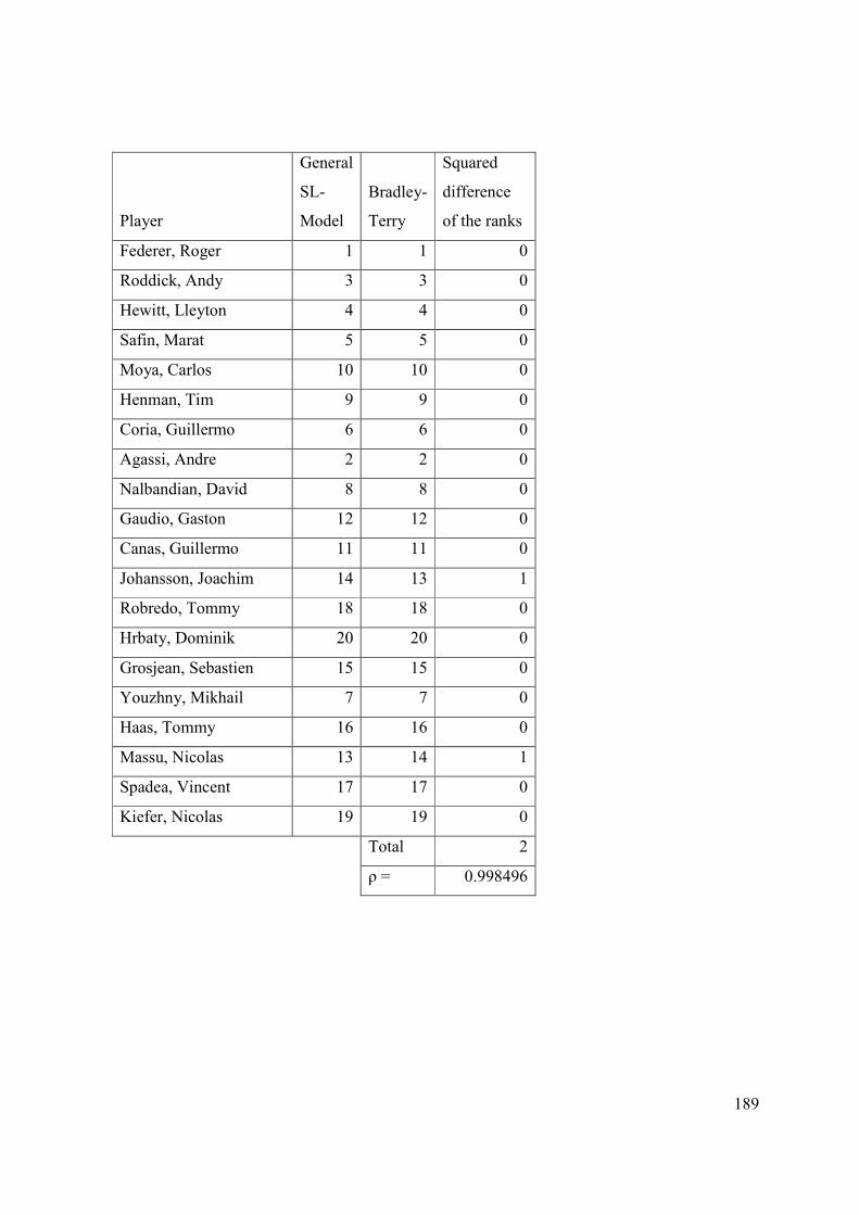
189

Player

General

SL-

Model

Bradley-

Terry

Squared

difference

of the ranks


Roddick, Andy 3 3 0


Safin, Marat 5 5 0


Henman, Tim 9 9 0


Agassi, Andre 2 2 0









Haas, Tommy 16 16 0




Total 2

ρ = 0.998496

190

nn

d6

13

n

1i

2

i

−−=ρ∑= = 0.998496




σ2 = 0.052632

z = 4.352344

α = 0.95


Reject H0.


between the ranks obtained by the SL-model and the ranks obtained by the Bradley-Terry

model.

7.7.7 General SL-Model vs Poisson Model

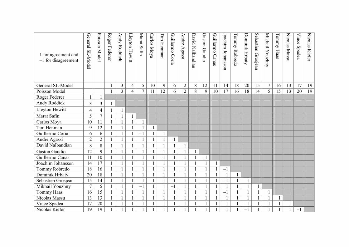
1 for agreement and


General S

L-M

odel

Poisso

n M

odel

Roger F

ederer

Andy Roddick

Lley

ton Hew

itt

Marat S

afin

Carlo

s Moya

Tim

Henman

Guillerm

o Coria

Andre A

gassi

David Nalb

andian

Gasto

n Gaudio

Guillerm

o Canas

Joach

im Jo

hansso

n

Tommy Robred

o

Dominik Hrbaty

Sebastien

Grosjean

Mikhail Y

ouzhny

Tommy Haas

Nico

las Massu

Vince S

padea

Nico

las Kiefer

General SL-Model 1 3 4 5 10 9 6 2 8 12 11 14 18 20 15 7 16 13 17 19

Poisson Model 1 3 4 7 11 12 6 2 8 9 10 17 16 18 14 5 15 13 20 19

Roger Federer 1 1

Andy Roddick 3 3 1




Tim Henman 9 12 1 1 1 1 –1


Andre Agassi 2 2 1 1 1 1 1 1 1


Gaston Gaudio 12 9 1 1 1 1 –1 –1 1 1 1

Guillermo Canas 11 10 1 1 1 1 –1 –1 1 1 1 –1


Tommy Robredo 18 16 1 1 1 1 1 1 1 1 1 1 1 –1

Dominik Hrbaty 20 18 1 1 1 1 1 1 1 1 1 1 1 1 1


Mikhail Youzhny 7 5 1 1 1 –1 1 1 –1 1 1 1 1 1 1 1 1

Tommy Haas 16 15 1 1 1 1 1 1 1 1 1 1 1 –1 1 1 1 1

Nicolas Massu 13 13 1 1 1 1 1 1 1 1 1 1 1 1 1 1 1 1 1

Vince Spadea 17 20 1 1 1 1 1 1 1 1 1 1 1 1 –1 –1 1 1 1 1

Nicolas Kiefer 19 19 1 1 1 1 1 1 1 1 1 1 1 1 1 –1 1 1 1 1 –1

192

−=



τ =∑

∑

<

<

ji

2

ij

ji

ij

a

a

= 0.83157895




σ2 = 950

S = 158

z = 5.12619691

α = 0.95


Reject H0.


between the ranks obtained by the general SL-model and the ranks obtained by the poisson

model.

193

Player

General

SL-

Model

Poisson

Model

Squared

difference

of the ranks


Roddick, Andy 3 3 0


Safin, Marat 5 7 4


Henman, Tim 9 12 9


Agassi, Andre 2 2 0









Haas, Tommy 16 15 1




Total 56

ρ = 0.957895

194

nn

d6

13

n

1i

2

i

−−=ρ∑= = 0.957895




σ2 = 0.052632

z = 4.175366

α = 0.95


Reject H0.


between the ranks obtained by the general SL-model and the ranks obtained by the poisson

model.

7.7.8 General SL-Model vs Approx. Algorithm of Bayesian Solution Poisson Model

1 for agreement and


General S

L-M

odel

Poisso

n Approx

Roger F

ederer

Andy Roddick

Lley

ton Hew

itt

Marat S

afin

Carlo

s Moya

Tim

Henman

Guillerm

o Coria

Andre A

gassi

David Nalb

andian

Gasto

n Gaudio

Guillerm

o Canas

Joach

im Jo

hansso

n

Tommy Robred

o

Dominik Hrbaty

Sebastien

Grosjean

Mikhail Y

ouzhny

Tommy Haas

Nico

las Massu

Vince S

padea

Nico

las Kiefer

General SL-Model 1 3 4 5 10 9 6 2 8 12 11 14 18 20 15 7 16 13 17 19

Poisson Approx 1 3 5 14 11 12 6 2 9 7 8 16 17 15 13 4 18 10 19 20

Roger Federer 1 1

Andy Roddick 3 3 1



Carlos Moya 10 11 1 1 1 –1

Tim Henman 9 12 1 1 1 –1 –1


Andre Agassi 2 2 1 1 1 1 1 1 1

David Nalbandian 8 9 1 1 1 –1 1 1 1 1

Gaston Gaudio 12 7 1 1 1 –1 –1 –1 1 1 –1

Guillermo Canas 11 8 1 1 1 –1 –1 –1 1 1 –1 –1


Tommy Robredo 18 17 1 1 1 1 1 1 1 1 1 1 1 1

Dominik Hrbaty 20 15 1 1 1 1 1 1 1 1 1 1 1 –1 –1

Sebastien Grosjean 15 13 1 1 1 –1 1 1 1 1 1 1 1 –1 1 1

Mikhail Youzhny 7 4 1 1 –1 –1 1 1 –1 1 1 1 1 1 1 1 1

Tommy Haas 16 18 1 1 1 1 1 1 1 1 1 1 1 1 –1 –1 1 1

Nicolas Massu 13 10 1 1 1 –1 –1 –1 1 1 1 1 1 1 1 1 1 1 1

Vince Spadea 17 19 1 1 1 1 1 1 1 1 1 1 1 1 –1 –1 1 1 1 1

Nicolas Kiefer 19 20 1 1 1 1 1 1 1 1 1 1 1 1 1 –1 1 1 1 1 1

196

−=



τ =∑

∑

<

<

ji

2

ij

ji

ij

a

a

= 0.69473684




σ2 = 950

S = 132

z = 4.28264552

α = 0.95


Reject H0.


between the ranks obtained by the general SL-model and the ranks obtained by the

approximate algorithm of the bayesian solution to the poisson model.

197

Player

General

SL-

Model

Poisson

Approx

Squared

difference

of the ranks


Roddick, Andy 3 3 0




Henman, Tim 9 12 9


Agassi, Andre 2 2 0









Haas, Tommy 16 18 4




Total 188

ρ = 0.858647

198

nn

d6

13

n

1i

2

i

−−=ρ∑= = 0.858647




σ2 = 0.052632

z = 3.742754

α = 0.95


Reject H0.


between the ranks obtained by the general SL-model and the ranks obtained by the


7.7.9 General SL-Model vs Row Sum Method

1 for agreement and


General S

L-M

odel

Row Sum M

ethod

Roger F

ederer

Andy Roddick

Lley

ton Hew

itt

Marat S

afin

Carlo

s Moya

Tim

Henman

Guillerm

o Coria

Andre A

gassi

David Nalb

andian

Gasto

n Gaudio

Guillerm

o Canas

Joach

im Jo

hansso

n

Tommy Robred

o

Dominik Hrbaty

Sebastien

Grosjean

Mikhail Y

ouzhny

Tommy Haas

Nico

las Massu

Vince S

padea

Nico

las Kiefer

General SL-Model 1 3 4 5 10 9 6 2 8 12 11 14 18 20 15 7 16 13 17 19

Row Sum Method 1 2 3 4 10 9 6 5 12 7 8 16 18 14 20 11 15 17 19 13

Roger Federer 1 1

Andy Roddick 3 2 1




Tim Henman 9 9 1 1 1 1 1


Andre Agassi 2 5 1 –1 –1 –1 1 1 1


Gaston Gaudio 12 7 1 1 1 1 –1 –1 1 1 –1

Guillermo Canas 11 8 1 1 1 1 –1 –1 1 1 –1 –1


Tommy Robredo 18 18 1 1 1 1 1 1 1 1 1 1 1 1

Dominik Hrbaty 20 14 1 1 1 1 1 1 1 1 1 1 1 –1 –1


Mikhail Youzhny 7 11 1 1 1 1 –1 –1 1 1 1 –1 –1 1 1 1 1

Tommy Haas 16 15 1 1 1 1 1 1 1 1 1 1 1 –1 1 –1 –1 1

Nicolas Massu 13 17 1 1 1 1 1 1 1 1 1 1 1 –1 1 –1 1 1 –1

Vince Spadea 17 19 1 1 1 1 1 1 1 1 1 1 1 1 –1 –1 –1 1 1 1

Nicolas Kiefer 19 13 1 1 1 1 1 1 1 1 1 1 1 –1 –1 1 –1 1 –1 –1 –1

200

−=



τ =∑

∑

<

<

ji

2

ij

ji

ij

a

a

= 0.63157895




σ2 = 950

S = 120

z = 3.89331411

α = 0.95


Reject H0.


between the ranks obtained by the general SL-model and the ranks obtained by the row sum

method.

201

Player

General

SL-

Model

Row

Sum

Method

Squared

difference

of the ranks


Roddick, Andy 3 2 1


Safin, Marat 5 4 1


Henman, Tim 9 9 0


Agassi, Andre 2 5 9









Haas, Tommy 16 15 1




Total 200

ρ = 0.849624

202

nn

d6

13

n

1i

2

i

−−=ρ∑= = 0.849624




σ2 = 0.052632

z = 3.703425

α = 0.95


Reject H0.


between the ranks obtained by the general SL-model and the ranks obtained by the row sum

method.

7.7.10 Binary SL-Model vs DDic01 Binary SL-Model

1 for agreement and


Bin SL-M

odel

DDic0

1 Bin SL-M

odel

Roger F

ederer

Andy Roddick

Lley

ton Hew

itt

Marat S

afin

Carlo

s Moya

Tim

Henman

Guillerm

o Coria

Andre A

gassi

David Nalb

andian

Gasto

n Gaudio

Guillerm

o Canas

Joach

im Jo

hansso

n

Tommy Robred

o

Dominik Hrbaty

Sebastien

Grosjean

Mikhail Y

ouzhny

Tommy Haas

Nico

las Massu

Vince S

padea

Nico

las Kiefer

Bin SL-Model 1 2 4 6 12 8 5 3 9 10 11 13 20 15 19 7 17 14 16 18

DDic01 Bin SL-Model 1 2 4 7 14 8 5 3 9 10 11 12 19 15 16 6 20 13 17 18

Roger Federer 1 1

Andy Roddick 2 2 1




Tim Henman 8 8 1 1 1 1 1


Andre Agassi 3 3 1 1 1 1 1 1 1


Gaston Gaudio 10 10 1 1 1 1 1 1 1 1 1

Guillermo Canas 11 11 1 1 1 1 1 1 1 1 1 1


Tommy Robredo 20 19 1 1 1 1 1 1 1 1 1 1 1 1

Dominik Hrbaty 15 15 1 1 1 1 1 1 1 1 1 1 1 1 1


Mikhail Youzhny 7 6 1 1 1 –1 1 1 1 1 1 1 1 1 1 1 1

Tommy Haas 17 20 1 1 1 1 1 1 1 1 1 1 1 1 –1 1 –1 1

Nicolas Massu 14 13 1 1 1 1 –1 1 1 1 1 1 1 1 1 1 1 1 1

Vince Spadea 16 17 1 1 1 1 1 1 1 1 1 1 1 1 1 1 –1 1 1 1

Nicolas Kiefer 18 18 1 1 1 1 1 1 1 1 1 1 1 1 1 1 –1 1 –1 1 1

204

−=



τ =∑

∑

<

<

ji

2

ij

ji

ij

a

a

= 0.91578947




σ2 = 950

S = 174

z = 5.64530546

α = 0.95


Reject H0.


between the ranks obtained by the binary SL-model and the ranks obtained by the DDic01

binary SL-model.

205

Player

Bin

SL-

Model

DDic01

Bin SL-

Model

Squared

difference

of the ranks


Roddick, Andy 2 2 0


Safin, Marat 6 7 1


Henman, Tim 8 8 0


Agassi, Andre 3 3 0









Haas, Tommy 17 20 9




Total 28

ρ = 0.978947

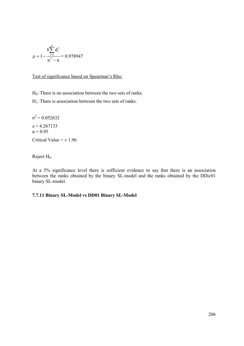
206

nn

d6

13

n

1i

2

i

−−=ρ∑= = 0.978947




σ2 = 0.052632

z = 4.267133

α = 0.95


Reject H0.


between the ranks obtained by the binary SL-model and the ranks obtained by the DDic01

binary SL-model.

7.7.11 Binary SL-Model vs DD01 Binary SL-Model

1 for agreement and


Bin SL-M

odel

DD01 Bin SL-M

odel

Roger F

ederer

Andy Roddick

Lley

ton Hew

itt

Marat S

afin

Carlo

s Moya

Tim

Henman

Guillerm

o Coria

Andre A

gassi

David Nalb

andian

Gasto

n Gaudio

Guillerm

o Canas

Joach

im Jo

hansso

n

Tommy Robred

o

Dominik Hrbaty

Sebastien

Grosjean

Mikhail Y

ouzhny

Tommy Haas

Nico

las Massu

Vince S

padea

Nico

las Kiefer

Bin SL-Model 1 2 4 6 12 8 5 3 9 10 11 13 20 15 19 7 17 14 16 18

DD01 Bin SL-Model 1 2 4 7 14 9 5 3 10 13 8 12 20 16 17 6 18 11 15 19

Roger Federer 1 1

Andy Roddick 2 2 1




Tim Henman 8 9 1 1 1 1 1


Andre Agassi 3 3 1 1 1 1 1 1 1


Gaston Gaudio 10 13 1 1 1 1 1 1 1 1 1

Guillermo Canas 11 8 1 1 1 1 1 –1 1 1 –1 –1


Tommy Robredo 20 20 1 1 1 1 1 1 1 1 1 1 1 1

Dominik Hrbaty 15 16 1 1 1 1 1 1 1 1 1 1 1 1 1


Mikhail Youzhny 7 6 1 1 1 –1 1 1 1 1 1 1 1 1 1 1 1

Tommy Haas 17 18 1 1 1 1 1 1 1 1 1 1 1 1 1 1 –1 1

Nicolas Massu 14 11 1 1 1 1 –1 1 1 1 1 –1 1 –1 1 1 1 1 1

Vince Spadea 16 15 1 1 1 1 1 1 1 1 1 1 1 1 1 –1 1 1 1 1

Nicolas Kiefer 18 19 1 1 1 1 1 1 1 1 1 1 1 1 1 1 –1 1 1 1 1

208

−=



τ =∑

∑

<

<

ji

2

ij

ji

ij

a

a

= 0.87368421




σ2 = 950

S = 166

z = 5.38575118

α = 0.95


Reject H0.


between the ranks obtained by the binary SL-model and the ranks obtained by the DD01 binary

SL-model.

209

Player

Bin

SL-

Model

DD01

Bin SL-

Model

Squared

difference

of the ranks


Roddick, Andy 2 2 0


Safin, Marat 6 7 1


Henman, Tim 8 9 1


Agassi, Andre 3 3 0









Haas, Tommy 17 18 1




Total 44

ρ = 0.966917

210

nn

d6

13

n

1i

2

i

−−=ρ∑= = 0.966917




σ2 = 0.052632

z = 4.214695

α = 0.95


Reject H0.


between the ranks obtained by the binary SL-model and the ranks obtained by the DD01 binary

SL-model.

7.7.12 Binary SL-Model vs Binomial Poisson Model (Bayesian Solution)

1 for agreement and


Bin SL-M

odel

Binomial P

oisso

n B

Roger F

ederer

Andy Roddick

Lley

ton Hew

itt

Marat S

afin

Carlo

s Moya

Tim

Henman

Guillerm

o Coria

Andre A

gassi

David Nalb

andian

Gasto

n Gaudio

Guillerm

o Canas

Joach

im Jo

hansso

n

Tommy Robred

o

Dominik Hrbaty

Sebastien

Grosjean

Mikhail Y

ouzhny

Tommy Haas

Nico

las Massu

Vince S

padea

Nico

las Kiefer

Bin SL-Model 1 2 4 6 12 8 5 3 9 10 11 13 20 15 19 7 17 14 16 18


Roger Federer 1 1

Andy Roddick 2 3 1




Tim Henman 8 8 1 1 1 1 1

Guillermo Coria 5 4 1 1 –1 1 1 1

Andre Agassi 3 2 1 –1 1 1 1 1 1


Gaston Gaudio 10 12 1 1 1 1 –1 1 1 1 1

Guillermo Canas 11 11 1 1 1 1 –1 1 1 1 1 –1


Tommy Robredo 20 19 1 1 1 1 1 1 1 1 1 1 1 1

Dominik Hrbaty 15 18 1 1 1 1 1 1 1 1 1 1 1 1 1

Sebastien Grosjean 19 13 1 1 1 1 1 1 1 1 1 1 1 –1 1 –1

Mikhail Youzhny 7 6 1 1 –1 1 1 1 1 1 1 1 1 1 1 1 1

Tommy Haas 17 14 1 1 1 1 1 1 1 1 1 1 1 –1 1 –1 –1 1

Nicolas Massu 14 16 1 1 1 1 1 1 1 1 1 1 1 1 1 1 –1 1 –1

Vince Spadea 16 20 1 1 1 1 1 1 1 1 1 1 1 1 –1 1 –1 1 –1 1

Nicolas Kiefer 18 17 1 1 1 1 1 1 1 1 1 1 1 1 1 –1 –1 1 1 1 –1

212

−=



τ =∑

∑

<

<

ji

2

ij

ji

ij

a

a

= 0.78947368




σ2 = 950

S = 150

z = 4.86664263

α = 0.95


Reject H0.


between the ranks obtained by the binary SL-model and the ranks obtained by the bayesian


213

Player

Bin

SL-

Model

Binomial

Poisson

B

Squared

difference

of the ranks


Roddick, Andy 2 3 1


Safin, Marat 6 5 1


Henman, Tim 8 8 0


Agassi, Andre 3 2 1









Haas, Tommy 17 14 9




Total 102

ρ = 0.923308

214

nn

d6

13

n

1i

2

i

−−=ρ∑= = 0.923308




σ2 = 0.052632

z = 4.024607

α = 0.95


Reject H0.


between the ranks obtained by the binary SL-model and the ranks obtained by the bayesian


7.7.13 Binary SL-Model vs Binomial Poisson Model (Max. Like. Solution)

1 for agreement and


Bin SL-M

odel

Binomial P

oisso

n M

L

Roger F

ederer

Andy Roddick

Lley

ton Hew

itt

Marat S

afin

Carlo

s Moya

Tim

Henman

Guillerm

o Coria

Andre A

gassi

David Nalb

andian

Gasto

n Gaudio

Guillerm

o Canas

Joach

im Jo

hansso

n

Tommy Robred

o

Dominik Hrbaty

Sebastien

Grosjean

Mikhail Y

ouzhny

Tommy Haas

Nico

las Massu

Vince S

padea

Nico

las Kiefer

Bin SL-Model 1 2 4 6 12 8 5 3 9 10 11 13 20 15 19 7 17 14 16 18


Roger Federer 1 1

Andy Roddick 2 3 1




Tim Henman 8 8 1 1 1 1 1


Andre Agassi 3 2 1 –1 1 1 1 1 1


Gaston Gaudio 10 13 1 1 1 1 –1 1 1 1 1

Guillermo Canas 11 11 1 1 1 1 –1 1 1 1 1 –1


Tommy Robredo 20 18 1 1 1 1 1 1 1 1 1 1 1 1

Dominik Hrbaty 15 20 1 1 1 1 1 1 1 1 1 1 1 1 –1


Mikhail Youzhny 7 7 1 1 1 1 1 1 1 1 1 1 1 1 1 1 1

Tommy Haas 17 16 1 1 1 1 1 1 1 1 1 1 1 1 1 –1 –1 1

Nicolas Massu 14 14 1 1 1 1 1 1 1 1 1 1 1 1 1 1 1 1 1

Vince Spadea 16 17 1 1 1 1 1 1 1 1 1 1 1 1 1 –1 –1 1 –1 1

Nicolas Kiefer 18 19 1 1 1 1 1 1 1 1 1 1 1 1 –1 –1 –1 1 1 1 1

216

−=



τ =∑

∑

<

<

ji

2

ij

ji

ij

a

a

= 0.83157895




σ2 = 950

S = 158

z = 5.12619691

α = 0.95


Reject H0.


between the ranks obtained by the binary SL-model and the ranks obtained by the maximum


217

Player

Bin

SL-

Model

Binomial

Poisson

ML

Squared

difference of

the ranks


Roddick, Andy 2 3 1


Safin, Marat 6 5 1


Henman, Tim 8 8 0


Agassi, Andre 3 2 1









Haas, Tommy 17 16 1




Total 66

ρ = 0.950376

218

nn

d6

13

n

1i

2

i

−−=ρ∑= = 0.950376




σ2 = 0.052632

z = 4.142593

α = 0.95


Reject H0.


between the ranks obtained by the binary SL-model and the ranks obtained by the maximum


7.7.14 Binary SL-Model vs Bradley-Terry Model

1 for agreement and


Bin SL-M

odel

Brad

ley-Terry

Roger F

ederer

Andy Roddick

Lley

ton Hew

itt

Marat S

afin

Carlo

s Moya

Tim

Henman

Guillerm

o Coria

Andre A

gassi

David Nalb

andian

Gasto

n Gaudio

Guillerm

o Canas

Joach

im Jo

hansso

n

Tommy Robred

o

Dominik Hrbaty

Sebastien

Grosjean

Mikhail Y

ouzhny

Tommy Haas

Nico

las Massu

Vince S

padea

Nico

las Kiefer

Bin SL-Model 1 2 4 6 12 8 5 3 9 10 11 13 20 15 19 7 17 14 16 18

Bradley-Terry 1 3 4 5 10 9 6 2 8 12 11 13 18 20 15 7 16 14 17 19

Roger Federer 1 1

Andy Roddick 2 3 1




Tim Henman 8 9 1 1 1 1 1


Andre Agassi 3 2 1 –1 1 1 1 1 1


Gaston Gaudio 10 12 1 1 1 1 –1 1 1 1 1

Guillermo Canas 11 11 1 1 1 1 –1 1 1 1 1 –1


Tommy Robredo 20 18 1 1 1 1 1 1 1 1 1 1 1 1

Dominik Hrbaty 15 20 1 1 1 1 1 1 1 1 1 1 1 1 –1


Mikhail Youzhny 7 7 1 1 1 1 1 1 1 1 1 1 1 1 1 1 1

Tommy Haas 17 16 1 1 1 1 1 1 1 1 1 1 1 1 1 –1 –1 1

Nicolas Massu 14 14 1 1 1 1 1 1 1 1 1 1 1 1 1 1 1 1 1

Vince Spadea 16 17 1 1 1 1 1 1 1 1 1 1 1 1 1 –1 –1 1 –1 1

Nicolas Kiefer 18 19 1 1 1 1 1 1 1 1 1 1 1 1 –1 –1 –1 1 1 1 1

220

−=



τ =∑

∑

<

<

ji

2

ij

ji

ij

a

a

= 0.83157895




σ2 = 950

S = 158

z = 5.12619691

α = 0.95


Reject H0.


between the ranks obtained by the binary SL-model and the ranks obtained by the Bradley-

Terry model.

221

Player

Bin

SL-

Model

Bradley-

Terry

Squared

difference

of the ranks


Roddick, Andy 2 3 1


Safin, Marat 6 5 1


Henman, Tim 8 9 1


Agassi, Andre 3 2 1









Haas, Tommy 17 16 1




Total 62

ρ = 0.953383

222

nn

d6

13

n

1i

2

i

−−=ρ∑= = 0.953383




σ2 = 0.052632

z = 4.155702

α = 0.95


Reject H0.


between the ranks obtained by the binary SL-model and the ranks obtained by the Bradley-

Terry model.

7.7.15 Binary SL-Model vs Poisson Model

1 for agreement and


Bin SL-M

odel

Poisso

n M

odel

Roger F

ederer

Andy Roddick

Lley

ton Hew

itt

Marat S

afin

Carlo

s Moya

Tim

Henman

Guillerm

o Coria

Andre A

gassi

David Nalb

andian

Gasto

n Gaudio

Guillerm

o Canas

Joach

im Jo

hansso

n

Tommy Robred

o

Dominik Hrbaty

Sebastien

Grosjean

Mikhail Y

ouzhny

Tommy Haas

Nico

las Massu

Vince S

padea

Nico

las Kiefer

Bin SL-Model 1 2 4 6 12 8 5 3 9 10 11 13 20 15 19 7 17 14 16 18

Poisson Model 1 3 4 7 11 12 6 2 8 9 10 17 16 18 14 5 15 13 20 19

Roger Federer 1 1

Andy Roddick 2 3 1




Tim Henman 8 12 1 1 1 1 –1


Andre Agassi 3 2 1 –1 1 1 1 1 1


Gaston Gaudio 10 9 1 1 1 1 1 –1 1 1 1

Guillermo Canas 11 10 1 1 1 1 1 –1 1 1 1 1


Tommy Robredo 20 16 1 1 1 1 1 1 1 1 1 1 1 –1

Dominik Hrbaty 15 18 1 1 1 1 1 1 1 1 1 1 1 1 –1


Mikhail Youzhny 7 5 1 1 1 –1 1 1 –1 1 1 1 1 1 1 1 1

Tommy Haas 17 15 1 1 1 1 1 1 1 1 1 1 1 –1 1 –1 –1 1

Nicolas Massu 14 13 1 1 1 1 1 1 1 1 1 1 1 –1 1 1 1 1 1

Vince Spadea 16 20 1 1 1 1 1 1 1 1 1 1 1 1 –1 1 –1 1 –1 1

Nicolas Kiefer 18 19 1 1 1 1 1 1 1 1 1 1 1 1 –1 1 –1 1 1 1 –1

224

−=



τ =∑

∑

<

<

ji

2

ij

ji

ij

a

a

= 0.77894737




σ2 = 950

S = 148

z = 4.80175407

α = 0.95


Reject H0.


between the ranks obtained by the binary SL-model and the ranks obtained by the poisson

model.

225

Player

Bin

SL-

Model

Poisson

Model

Squared

difference

of the ranks


Roddick, Andy 2 3 1


Safin, Marat 6 7 1


Henman, Tim 8 12 16


Agassi, Andre 3 2 1









Haas, Tommy 17 15 4




Total 116

ρ = 0.912782

226

nn

d6

13

n

1i

2

i

−−=ρ∑= = 0.912782




σ2 = 0.052632

z = 3.978724

α = 0.95


Reject H0.


between the ranks obtained by the binary SL-model and the ranks obtained by the poisson

model.

7.7.16 Binary SL-Model vs Approx. Algorithm of Bayesian Solution Poisson Model

1 for agreement and


Bin SL-M

odel

Poisso

n Approx

Roger F

ederer

Andy Roddick

Lley

ton Hew

itt

Marat S

afin

Carlo

s Moya

Tim

Henman

Guillerm

o Coria

Andre A

gassi

David Nalb

andian

Gasto

n Gaudio

Guillerm

o Canas

Joach

im Jo

hansso

n

Tommy Robred

o

Dominik Hrbaty

Sebastien

Grosjean

Mikhail Y

ouzhny

Tommy Haas

Nico

las Massu

Vince S

padea

Nico

las Kiefer

Bin SL-Model 1 2 4 6 12 8 5 3 9 10 11 13 20 15 19 7 17 14 16 18

Poisson Approx 1 3 5 14 11 12 6 2 9 7 8 16 17 15 13 4 18 10 19 20

Roger Federer 1 1

Andy Roddick 2 3 1



Carlos Moya 12 11 1 1 1 –1

Tim Henman 8 12 1 1 1 –1 –1


Andre Agassi 3 2 1 –1 1 1 1 1 1

David Nalbandian 9 9 1 1 1 –1 1 –1 1 1

Gaston Gaudio 10 7 1 1 1 –1 1 –1 1 1 –1

Guillermo Canas 11 8 1 1 1 –1 1 –1 1 1 –1 1


Tommy Robredo 20 17 1 1 1 1 1 1 1 1 1 1 1 1

Dominik Hrbaty 15 15 1 1 1 1 1 1 1 1 1 1 1 –1 1

Sebastien Grosjean 19 13 1 1 1 –1 1 1 1 1 1 1 1 –1 1 –1

Mikhail Youzhny 7 4 1 1 –1 –1 1 1 –1 1 1 1 1 1 1 1 1

Tommy Haas 17 18 1 1 1 1 1 1 1 1 1 1 1 1 –1 1 –1 1

Nicolas Massu 14 10 1 1 1 –1 –1 –1 1 1 1 1 1 –1 1 1 1 1 1

Vince Spadea 16 19 1 1 1 1 1 1 1 1 1 1 1 1 –1 1 –1 1 –1 1

Nicolas Kiefer 18 20 1 1 1 1 1 1 1 1 1 1 1 1 –1 1 –1 1 1 1 1

228

−=



τ =∑

∑

<

<

ji

2

ij

ji

ij

a

a

= 0.68421053




σ2 = 950

S = 130

z = 4.21775695

α = 0.95


Reject H0.


between the ranks obtained by the binary SL-model and the ranks obtained by the approximate

algorithm of the bayesian solution to the poisson model.

229

Player

Bin

SL-

Model

Poisson

Approx

Squared

difference

of the ranks


Roddick, Andy 2 3 1




Henman, Tim 8 12 16


Agassi, Andre 3 2 1









Haas, Tommy 17 18 1




Total 196

ρ = 0.852632

230

nn

d6

13

n

1i

2

i

−−=ρ∑= = 0.852632




σ2 = 0.052632

z = 3.716535

α = 0.95


Reject H0.


between the ranks obtained by the binary SL-model and the ranks obtained by the approximate


7.7.17 Binary SL-Model vs Row Sum Method

1 for agreement and


Bin SL-M

odel

Row Sum M

ethod

Roger F

ederer

Andy Roddick

Lley

ton Hew

itt

Marat S

afin

Carlo

s Moya

Tim

Henman

Guillerm

o Coria

Andre A

gassi

David Nalb

andian

Gasto

n Gaudio

Guillerm

o Canas

Joach

im Jo

hansso

n

Tommy Robred

o

Dominik Hrbaty

Sebastien

Grosjean

Mikhail Y

ouzhny

Tommy Haas

Nico

las Massu

Vince S

padea

Nico

las Kiefer

Bin SL-Model 1 2 4 6 12 8 5 3 9 10 11 13 20 15 19 7 17 14 16 18

Row Sum Method 1 2 3 4 10 9 6 5 12 7 8 16 18 14 20 11 15 17 19 13

Roger Federer 1 1

Andy Roddick 2 2 1




Tim Henman 8 9 1 1 1 1 1


Andre Agassi 3 5 1 1 –1 –1 1 1 1


Gaston Gaudio 10 7 1 1 1 1 1 –1 1 1 –1

Guillermo Canas 11 8 1 1 1 1 1 –1 1 1 –1 1


Tommy Robredo 20 18 1 1 1 1 1 1 1 1 1 1 1 1

Dominik Hrbaty 15 14 1 1 1 1 1 1 1 1 1 1 1 –1 1


Mikhail Youzhny 7 11 1 1 1 1 –1 –1 1 1 1 –1 –1 1 1 1 1

Tommy Haas 17 15 1 1 1 1 1 1 1 1 1 1 1 –1 1 1 1 1

Nicolas Massu 14 17 1 1 1 1 1 1 1 1 1 1 1 1 1 –1 1 1 –1

Vince Spadea 16 19 1 1 1 1 1 1 1 1 1 1 1 1 –1 1 1 1 –1 1

Nicolas Kiefer 18 13 1 1 1 1 1 1 1 1 1 1 1 –1 1 –1 1 1 –1 –1 –1

232

−=



τ =∑

∑

<

<

ji

2

ij

ji

ij

a

a

= 0.74736842




σ2 = 950

S = 142

z = 4.60708836

α = 0.95


Reject H0.


between the ranks obtained by the binary SL-model and the ranks obtained by the row sum

method.

233

Player

Bin

SL-

Model

Row

Sum

Method

Squared

difference

of the ranks


Roddick, Andy 2 2 0


Safin, Marat 6 4 4


Henman, Tim 8 9 1


Agassi, Andre 3 5 4









Haas, Tommy 17 15 4




Total 120

ρ = 0.909774

234

nn

d6

13

n

1i

2

i

−−=ρ∑= = 0.909774




σ2 = 0.052632

z = 3.965615

α = 0.95


Reject H0.


between the ranks obtained by the binary SL-model and the ranks obtained by the row sum

method.

7.7.18 DDic01 Binary SL-Model vs DD01 Binary SL-Model

1 for agreement and


DDic0

1 Bin SL-M

odel

DD01 Bin SL-M

odel

Roger F

ederer

Andy Roddick

Lley

ton Hew

itt

Marat S

afin

Carlo

s Moya

Tim

Henman

Guillerm

o Coria

Andre A

gassi

David Nalb

andian

Gasto

n Gaudio

Guillerm

o Canas

Joach

im Jo

hansso

n

Tommy Robred

o

Dominik Hrbaty

Sebastien

Grosjean

Mikhail Y

ouzhny

Tommy Haas

Nico

las Massu

Vince S

padea

Nico

las Kiefer

DDic01 Bin SL-Model 1 2 4 7 14 8 5 3 9 10 11 12 19 15 16 6 20 13 17 18

DD01 Bin SL-Model 1 2 4 7 14 9 5 3 10 13 8 12 20 16 17 6 18 11 15 19

Roger Federer 1 1

Andy Roddick 2 2 1




Tim Henman 8 9 1 1 1 1 1


Andre Agassi 3 3 1 1 1 1 1 1 1


Gaston Gaudio 10 13 1 1 1 1 1 1 1 1 1

Guillermo Canas 11 8 1 1 1 1 1 –1 1 1 –1 –1


Tommy Robredo 19 20 1 1 1 1 1 1 1 1 1 1 1 1

Dominik Hrbaty 15 16 1 1 1 1 1 1 1 1 1 1 1 1 1


Mikhail Youzhny 6 6 1 1 1 1 1 1 1 1 1 1 1 1 1 1 1

Tommy Haas 20 18 1 1 1 1 1 1 1 1 1 1 1 1 –1 1 1 1

Nicolas Massu 13 11 1 1 1 1 1 1 1 1 1 –1 1 –1 1 1 1 1 1

Vince Spadea 17 15 1 1 1 1 1 1 1 1 1 1 1 1 1 –1 –1 1 1 1

Nicolas Kiefer 18 19 1 1 1 1 1 1 1 1 1 1 1 1 1 1 1 1 –1 1 1

236

−=



τ =∑

∑

<

<

ji

2

ij

ji

ij

a

a

= 0.89473684




σ2 = 950

S = 170

z = 5.51552832

α = 0.95


Reject H0.


between the ranks obtained by the DDic01 binary SL-model and the ranks obtained by the

DD01 binary SL-model.

237

Player

DDic01

Bin SL-

Model

DD01

Bin SL-

Model

Squared

difference

of the ranks


Roddick, Andy 2 2 0


Safin, Marat 7 7 0


Henman, Tim 8 9 1


Agassi, Andre 3 3 0









Haas, Tommy 20 18 4




Total 36

ρ = 0.972932

238

nn

d6

13

n

1i

2

i

−−=ρ∑= = 0.972932




σ2 = 0.052632

z = 4.240914

α = 0.95


Reject H0.



DD01 binary SL-model.

7.7.19 DDic01 Binary SL-Model vs Binomial Poisson Model (Bayesian Solution)

1 for agreement and


DDic0

1 Bin SL-M

odel

Binomial P

oisso

n B

Roger F

ederer

Andy Roddick

Lley

ton Hew

itt

Marat S

afin

Carlo

s Moya

Tim

Henman

Guillerm

o Coria

Andre A

gassi

David Nalb

andian

Gasto

n Gaudio

Guillerm

o Canas

Joach

im Jo

hansso

n

Tommy Robred

o

Dominik Hrbaty

Sebastien

Grosjean

Mikhail Y

ouzhny

Tommy Haas

Nico

las Massu

Vince S

padea

Nico

las Kiefer

DDic01 Bin SL-Model 1 2 4 7 14 8 5 3 9 10 11 12 19 15 16 6 20 13 17 18


Roger Federer 1 1

Andy Roddick 2 3 1




Tim Henman 8 8 1 1 1 1 1


Andre Agassi 3 2 1 –1 1 1 1 1 1


Gaston Gaudio 10 12 1 1 1 1 –1 1 1 1 1

Guillermo Canas 11 11 1 1 1 1 –1 1 1 1 1 –1


Tommy Robredo 19 19 1 1 1 1 1 1 1 1 1 1 1 1

Dominik Hrbaty 15 18 1 1 1 1 1 1 1 1 1 1 1 1 1


Mikhail Youzhny 6 6 1 1 –1 –1 1 1 1 1 1 1 1 1 1 1 1

Tommy Haas 20 14 1 1 1 1 1 1 1 1 1 1 1 –1 –1 –1 1 1

Nicolas Massu 13 16 1 1 1 1 –1 1 1 1 1 1 1 1 1 1 –1 1 –1

Vince Spadea 17 20 1 1 1 1 1 1 1 1 1 1 1 1 –1 1 1 1 –1 1

Nicolas Kiefer 18 17 1 1 1 1 1 1 1 1 1 1 1 1 1 –1 1 1 –1 1 –1

240

−=



τ =∑

∑

<

<

ji

2

ij

ji

ij

a

a

= 0.76842105




σ2 = 950

S = 146

z = 4.7368655

α = 0.95


Reject H0.



bayesian binomial poisson model.

241

Player

DDic01

Bin SL-

Model

Binomial

Poisson B

Squared

difference

of the ranks


Roddick, Andy 2 3 1


Safin, Marat 7 5 4


Henman, Tim 8 8 0


Agassi, Andre 3 2 1













Total 118

ρ = 0.911278

242

nn

d6

13

n

1i

2

i

−−=ρ∑= = 0.911278




σ2 = 0.052632

z = 3.97217

α = 0.95


Reject H0.




7.7.20 DDic01 Binary SL-Model vs Binomial Poisson Model (Max. Like. Solution)

1 for agreement and


DDic0

1 Bin SL-M

odel

Binomial P

oisso

n M

L

Roger F

ederer

Andy Roddick

Lley

ton Hew

itt

Marat S

afin

Carlo

s Moya

Tim

Henman

Guillerm

o Coria

Andre A

gassi

David Nalb

andian

Gasto

n Gaudio

Guillerm

o Canas

Joach

im Jo

hansso

n

Tommy Robred

o

Dominik Hrbaty

Sebastien

Grosjean

Mikhail Y

ouzhny

Tommy Haas

Nico

las Massu

Vince S

padea

Nico

las Kiefer

DDic01 Bin SL-Model 1 2 4 7 14 8 5 3 9 10 11 12 19 15 16 6 20 13 17 18


Roger Federer 1 1

Andy Roddick 2 3 1




Tim Henman 8 8 1 1 1 1 1


Andre Agassi 3 2 1 –1 1 1 1 1 1


Gaston Gaudio 10 13 1 1 1 1 –1 1 1 1 1

Guillermo Canas 11 11 1 1 1 1 –1 1 1 1 1 –1


Tommy Robredo 19 18 1 1 1 1 1 1 1 1 1 1 1 1

Dominik Hrbaty 15 20 1 1 1 1 1 1 1 1 1 1 1 1 –1


Mikhail Youzhny 6 7 1 1 1 –1 1 1 1 1 1 1 1 1 1 1 1

Tommy Haas 20 16 1 1 1 1 1 1 1 1 1 1 1 1 –1 –1 1 1

Nicolas Massu 13 14 1 1 1 1 –1 1 1 1 1 1 1 1 1 1 1 1 1

Vince Spadea 17 17 1 1 1 1 1 1 1 1 1 1 1 1 1 –1 1 1 –1 1

Nicolas Kiefer 18 19 1 1 1 1 1 1 1 1 1 1 1 1 –1 –1 1 1 –1 1 1

244

−=



τ =∑

∑

<

<

ji

2

ij

ji

ij

a

a

= 0.81052632




σ2 = 950

S = 154

z = 4.99641977

α = 0.95


Reject H0.



maximum likelihood binomial poisson model.

245

Player

DDic01

Bin SL-

Model

Binomial

Poisson ML

Squared

difference of

the ranks


Roddick, Andy 2 3 1


Safin, Marat 7 5 4


Henman, Tim 8 8 0


Agassi, Andre 3 2 1













Total 78

ρ = 0.941353

246

nn

d6

13

n

1i

2

i

−−=ρ∑= = 0.941353




σ2 = 0.052632

z = 4.103264

α = 0.95


Reject H0.




7.7.21 DDic01 Binary SL-Model vs Bradley-Terry Model

1 for agreement and


DDic0

1 Bin SL-M

odel

Brad

ley-Terry

Roger F

ederer

Andy Roddick

Lley

ton Hew

itt

Marat S

afin

Carlo

s Moya

Tim

Henman

Guillerm

o Coria

Andre A

gassi

David Nalb

andian

Gasto

n Gaudio

Guillerm

o Canas

Joach

im Jo

hansso

n

Tommy Robred

o

Dominik Hrbaty

Sebastien

Grosjean

Mikhail Y

ouzhny

Tommy Haas

Nico

las Massu

Vince S

padea

Nico

las Kiefer

DDic01 Bin SL-Model 1 2 4 7 14 8 5 3 9 10 11 12 19 15 16 6 20 13 17 18

Bradley-Terry 1 3 4 5 10 9 6 2 8 12 11 13 18 20 15 7 16 14 17 19

Roger Federer 1 1

Andy Roddick 2 3 1




Tim Henman 8 9 1 1 1 1 1


Andre Agassi 3 2 1 –1 1 1 1 1 1


Gaston Gaudio 10 12 1 1 1 1 –1 1 1 1 1

Guillermo Canas 11 11 1 1 1 1 –1 1 1 1 1 –1


Tommy Robredo 19 18 1 1 1 1 1 1 1 1 1 1 1 1

Dominik Hrbaty 15 20 1 1 1 1 1 1 1 1 1 1 1 1 –1


Mikhail Youzhny 6 7 1 1 1 –1 1 1 1 1 1 1 1 1 1 1 1

Tommy Haas 20 16 1 1 1 1 1 1 1 1 1 1 1 1 –1 –1 1 1

Nicolas Massu 13 14 1 1 1 1 –1 1 1 1 1 1 1 1 1 1 1 1 1

Vince Spadea 17 17 1 1 1 1 1 1 1 1 1 1 1 1 1 –1 1 1 –1 1

Nicolas Kiefer 18 19 1 1 1 1 1 1 1 1 1 1 1 1 –1 –1 1 1 –1 1 1

248

−=



τ =∑

∑

<

<

ji

2

ij

ji

ij

a

a

= 0.81052632




σ2 = 950

S = 154

z = 4.99641977

α = 0.95


Reject H0.



Bradley-Terry model.

249

Player

DDic01

Bin SL-

Model

Bradley-

Terry

Squared

difference

of the ranks


Roddick, Andy 2 3 1


Safin, Marat 7 5 4


Henman, Tim 8 9 1


Agassi, Andre 3 2 1













Total 76

ρ = 0.942857

250

nn

d6

13

n

1i

2

i

−−=ρ∑= = 0.942857




σ2 = 0.052632

z = 4.109819

α = 0.95


Reject H0.




7.7.22 DDic01 Binary SL-Model vs Poisson Model

1 for agreement and


DDic0

1 Bin SL-M

odel

Poisso

n M

odel

Roger F

ederer

Andy Roddick

Lley

ton Hew

itt

Marat S

afin

Carlo

s Moya

Tim

Henman

Guillerm

o Coria

Andre A

gassi

David Nalb

andian

Gasto

n Gaudio

Guillerm

o Canas

Joach

im Jo

hansso

n

Tommy Robred

o

Dominik Hrbaty

Sebastien

Grosjean

Mikhail Y

ouzhny

Tommy Haas

Nico

las Massu

Vince S

padea

Nico

las Kiefer

DDic01 Bin SL-Model 1 2 4 7 14 8 5 3 9 10 11 12 19 15 16 6 20 13 17 18

Poisson Model 1 3 4 7 11 12 6 2 8 9 10 17 16 18 14 5 15 13 20 19

Roger Federer 1 1

Andy Roddick 2 3 1




Tim Henman 8 12 1 1 1 1 –1


Andre Agassi 3 2 1 –1 1 1 1 1 1


Gaston Gaudio 10 9 1 1 1 1 1 –1 1 1 1

Guillermo Canas 11 10 1 1 1 1 1 –1 1 1 1 1


Tommy Robredo 19 16 1 1 1 1 1 1 1 1 1 1 1 –1

Dominik Hrbaty 15 18 1 1 1 1 1 1 1 1 1 1 1 1 –1


Mikhail Youzhny 6 5 1 1 1 1 1 1 –1 1 1 1 1 1 1 1 1

Tommy Haas 20 15 1 1 1 1 1 1 1 1 1 1 1 –1 –1 –1 1 1

Nicolas Massu 13 13 1 1 1 1 –1 1 1 1 1 1 1 –1 1 1 1 1 1

Vince Spadea 17 20 1 1 1 1 1 1 1 1 1 1 1 1 –1 1 1 1 –1 1

Nicolas Kiefer 18 19 1 1 1 1 1 1 1 1 1 1 1 1 –1 1 1 1 –1 1 –1

252

−=



τ =∑

∑

<

<

ji

2

ij

ji

ij

a

a

= 0.77894737




σ2 = 950

S = 148

z = 4.80175407

α = 0.95


Reject H0.



poisson model.

253

Player

DDic01

Bin SL-

Model

Poisson

Model

Squared

difference

of the ranks


Roddick, Andy 2 3 1


Safin, Marat 7 7 0


Henman, Tim 8 12 16


Agassi, Andre 3 2 1













Total 114

ρ = 0.914286

254

nn

d6

13

n

1i

2

i

−−=ρ∑= = 0.914286




σ2 = 0.052632

z = 3.985279

α = 0.95


Reject H0.



poisson model.

7.7.23 DDic01 Binary SL-Model vs Approx. Algorithm of Bayesian Solution Poisson

Model

1 for agreement and


DDic0

1 Bin SL-M

odel

Poisso

n Approx

Roger F

ederer

Andy Roddick

Lley

ton Hew

itt

Marat S

afin

Carlo

s Moya

Tim

Henman

Guillerm

o Coria

Andre A

gassi

David Nalb

andian

Gasto

n Gaudio

Guillerm

o Canas

Joach

im Jo

hansso

n

Tommy Robred

o

Dominik Hrbaty

Sebastien

Grosjean

Mikhail Y

ouzhny

Tommy Haas

Nico

las Massu

Vince S

padea

Nico

las Kiefer

DDic01 Bin SL-Model 1 2 4 7 14 8 5 3 9 10 11 12 19 15 16 6 20 13 17 18

Poisson Approx 1 3 5 14 11 12 6 2 9 7 8 16 17 15 13 4 18 10 19 20

Roger Federer 1 1

Andy Roddick 2 3 1



Carlos Moya 14 11 1 1 1 –1

Tim Henman 8 12 1 1 1 –1 –1


Andre Agassi 3 2 1 –1 1 1 1 1 1


Gaston Gaudio 10 7 1 1 1 –1 1 –1 1 1 –1

Guillermo Canas 11 8 1 1 1 –1 1 –1 1 1 –1 1


Tommy Robredo 19 17 1 1 1 1 1 1 1 1 1 1 1 1

Dominik Hrbaty 15 15 1 1 1 1 1 1 1 1 1 1 1 –1 1


Mikhail Youzhny 6 4 1 1 –1 1 1 1 –1 1 1 1 1 1 1 1 1

Tommy Haas 20 18 1 1 1 1 1 1 1 1 1 1 1 1 1 1 1 1

Nicolas Massu 13 10 1 1 1 –1 1 –1 1 1 1 1 1 –1 1 1 1 1 1

Vince Spadea 17 19 1 1 1 1 1 1 1 1 1 1 1 1 –1 1 1 1 –1 1

Nicolas Kiefer 18 19 1 1 1 1 1 1 1 1 1 1 1 1 –1 1 1 1 –1 1 –1

256

−=



τ =∑

∑

<

<

ji

2

ij

ji

ij

a

a

= 0.72631579




σ2 = 950

S = 138

z = 4.47731122

α = 0.95


Reject H0.




257

Player

DDic01

Bin SL-

Model

Poisson

Approx

Squared

difference

of the ranks


Roddick, Andy 2 3 1




Henman, Tim 8 12 16


Agassi, Andre 3 2 1









Haas, Tommy 20 18 4




Total 150

ρ = 0.887218

258

nn

d6

13

n

1i

2

i

−−=ρ∑= = 0.887218




σ2 = 0.052632

z = 3.867294

α = 0.95


Reject H0.




7.7.24 DDic01 Binary SL-Model vs Row Sum Method

1 for agreement and


DDic0

1 Bin SL-M

odel

Row Sum M

ethod

Roger F

ederer

Andy Roddick

Lley

ton Hew

itt

Marat S

afin

Carlo

s Moya

Tim

Henman

Guillerm

o Coria

Andre A

gassi

David Nalb

andian

Gasto

n Gaudio

Guillerm

o Canas

Joach

im Jo

hansso

n

Tommy Robred

o

Dominik Hrbaty

Sebastien

Grosjean

Mikhail Y

ouzhny

Tommy Haas

Nico

las Massu

Vince S

padea

Nico

las Kiefer

DDic01 Bin SL-Model 1 2 4 7 14 8 5 3 9 10 11 12 19 15 16 6 20 13 17 18

Row Sum Method 1 2 3 4 10 9 6 5 12 7 8 16 18 14 20 11 15 17 19 13

Roger Federer 1 1

Andy Roddick 2 2 1




Tim Henman 8 9 1 1 1 1 1


Andre Agassi 3 5 1 1 –1 –1 1 1 1


Gaston Gaudio 10 7 1 1 1 1 1 –1 1 1 –1

Guillermo Canas 11 8 1 1 1 1 1 –1 1 1 –1 1


Tommy Robredo 19 18 1 1 1 1 1 1 1 1 1 1 1 1

Dominik Hrbaty 15 14 1 1 1 1 1 1 1 1 1 1 1 –1 1


Mikhail Youzhny 6 11 1 1 1 –1 –1 –1 1 1 1 –1 –1 1 1 1 1

Tommy Haas 20 15 1 1 1 1 1 1 1 1 1 1 1 –1 –1 1 –1 1

Nicolas Massu 13 17 1 1 1 1 –1 1 1 1 1 1 1 1 1 –1 1 1 –1

Vince Spadea 17 19 1 1 1 1 1 1 1 1 1 1 1 1 –1 1 –1 1 –1 1

Nicolas Kiefer 18 13 1 1 1 1 1 1 1 1 1 1 1 –1 1 –1 –1 1 1 –1 –1

260

−=



τ =∑

∑

<

<

ji

2

ij

ji

ij

a

a

= 0.68421053




σ2 = 950

S = 130

z = 4.21775695

α = 0.95


Reject H0.


between the ranks obtained by the DDic01 binary SL-model and the ranks obtained by the row

sum method.

261

Player

DDic01

Bin SL-

Model

Row Sum

Method

Squared

difference

of the ranks


Roddick, Andy 2 2 0


Safin, Marat 7 4 9


Henman, Tim 8 9 1


Agassi, Andre 3 5 4













Total 188

ρ = 0.858647

262

nn

d6

13

n

1i

2

i

−−=ρ∑= = 0.858647




σ2 = 0.052632

z = 3.742754

α = 0.95


Reject H0.


between the ranks obtained by the DDic01 binary SL-model and the ranks obtained by the row

sum method.

7.7.25 DD01 Binary SL-Model vs Binomial Poisson Model (Bayesian Solution)

1 for agreement and


DD01 Bin SL-M

odel

Binomial P

oisso

n B

Roger F

ederer

Andy Roddick

Lley

ton Hew

itt

Marat S

afin

Carlo

s Moya

Tim

Henman

Guillerm

o Coria

Andre A

gassi

David Nalb

andian

Gasto

n Gaudio

Guillerm

o Canas

Joach

im Jo

hansso

n

Tommy Robred

o

Dominik Hrbaty

Sebastien

Grosjean

Mikhail Y

ouzhny

Tommy Haas

Nico

las Massu

Vince S

padea

Nico

las Kiefer

DD01 Bin SL-Model 1 2 4 7 14 9 5 3 10 13 8 12 20 16 17 6 18 11 15 19


Roger Federer 1 1

Andy Roddick 2 3 1




Tim Henman 9 8 1 1 1 1 1


Andre Agassi 3 2 1 –1 1 1 1 1 1


Gaston Gaudio 13 12 1 1 1 1 –1 1 1 1 1

Guillermo Canas 8 11 1 1 1 1 –1 –1 1 1 –1 1


Tommy Robredo 20 19 1 1 1 1 1 1 1 1 1 1 1 1

Dominik Hrbaty 16 18 1 1 1 1 1 1 1 1 1 1 1 1 1


Mikhail Youzhny 6 6 1 1 –1 –1 1 1 1 1 1 1 1 1 1 1 1

Tommy Haas 18 14 1 1 1 1 1 1 1 1 1 1 1 –1 1 –1 1 1

Nicolas Massu 11 16 1 1 1 1 –1 1 1 1 1 –1 1 –1 1 1 –1 1 –1

Vince Spadea 15 20 1 1 1 1 1 1 1 1 1 1 1 1 –1 –1 –1 1 –1 1

Nicolas Kiefer 19 17 1 1 1 1 1 1 1 1 1 1 1 1 1 –1 1 1 1 1 –1

264

−=



τ =∑

∑

<

<

ji

2

ij

ji

ij

a

a

= 0.72631579




σ2 = 950

S = 138

z = 4.47731122

α = 0.95


Reject H0.


between the ranks obtained by the DD01 binary SL-model and the ranks obtained by the


265

Player

DD01

Bin SL-

Model

Binomial

Poisson B

Squared

difference of

the ranks


Roddick, Andy 2 3 1


Safin, Marat 7 5 4


Henman, Tim 9 8 1


Agassi, Andre 3 2 1













Total 144

ρ = 0.891729

266

nn

d6

13

n

1i

2

i

−−=ρ∑= = 0.891729




σ2 = 0.052632

z = 3.886958

α = 0.95


Reject H0.




7.7.26 DD01 Binary SL-Model vs Binomial Poisson Model (Max. Like. Solution)

1 for agreement and


DD01 Bin SL-M

odel

Binomial P

oisso

n M

L

Roger F

ederer

Andy Roddick

Lley

ton Hew

itt

Marat S

afin

Carlo

s Moya

Tim

Henman

Guillerm

o Coria

Andre A

gassi

David Nalb

andian

Gasto

n Gaudio

Guillerm

o Canas

Joach

im Jo

hansso

n

Tommy Robred

o

Dominik Hrbaty

Sebastien

Grosjean

Mikhail Y

ouzhny

Tommy Haas

Nico

las Massu

Vince S

padea

Nico

las Kiefer

DD01 Bin SL-Model 1 2 4 7 14 9 5 3 10 13 8 12 20 16 17 6 18 11 15 19


Roger Federer 1 1

Andy Roddick 2 3 1




Tim Henman 9 8 1 1 1 1 1


Andre Agassi 3 2 1 –1 1 1 1 1 1


Gaston Gaudio 13 13 1 1 1 1 –1 1 1 1 1

Guillermo Canas 8 11 1 1 1 1 –1 –1 1 1 –1 1


Tommy Robredo 20 18 1 1 1 1 1 1 1 1 1 1 1 1

Dominik Hrbaty 16 20 1 1 1 1 1 1 1 1 1 1 1 1 –1


Mikhail Youzhny 6 7 1 1 1 –1 1 1 1 1 1 1 1 1 1 1 1

Tommy Haas 18 16 1 1 1 1 1 1 1 1 1 1 1 1 1 –1 1 1

Nicolas Massu 11 14 1 1 1 1 –1 1 1 1 1 –1 1 –1 1 1 1 1 1

Vince Spadea 15 17 1 1 1 1 1 1 1 1 1 1 1 1 1 1 –1 1 –1 1

Nicolas Kiefer 19 19 1 1 1 1 1 1 1 1 1 1 1 1 –1 –1 1 1 1 1 1

268

−=



τ =∑

∑

<

<

ji

2

ij

ji

ij

a

a

= 0.81052632




σ2 = 950

S = 154

z = 4.99641977

α = 0.95


Reject H0.




269

Player

DD01

Bin SL-

Model

Binomial

Poisson

ML

Squared

difference of

the ranks


Roddick, Andy 2 3 1


Safin, Marat 7 5 4


Henman, Tim 9 8 1


Agassi, Andre 3 2 1









Haas, Tommy 18 16 4




Total 76

ρ = 0.942857

270

nn

d6

13

n

1i

2

i

−−=ρ∑= = 0.942857




σ2 = 0.052632

z = 4.109819

α = 0.95


Reject H0.




7.7.27 DD01 Binary SL-Model vs Bradley-Terry Model

1 for agreement and


DD01 Bin SL-M

odel

Brad

ley-Terry

Roger F

ederer

Andy Roddick

Lley

ton Hew

itt

Marat S

afin

Carlo

s Moya

Tim

Henman

Guillerm

o Coria

Andre A

gassi

David Nalb

andian

Gasto

n Gaudio

Guillerm

o Canas

Joach

im Jo

hansso

n

Tommy Robred

o

Dominik Hrbaty

Sebastien

Grosjean

Mikhail Y

ouzhny

Tommy Haas

Nico

las Massu

Vince S

padea

Nico

las Kiefer

DD01 Bin SL-Model 1 2 4 7 14 9 5 3 10 13 8 12 20 16 17 6 18 11 15 19

Bradley-Terry 1 3 4 5 10 9 6 2 8 12 11 13 18 20 15 7 16 14 17 19

Roger Federer 1 1

Andy Roddick 2 3 1




Tim Henman 9 9 1 1 1 1 1


Andre Agassi 3 2 1 –1 1 1 1 1 1


Gaston Gaudio 13 12 1 1 1 1 –1 1 1 1 1

Guillermo Canas 8 11 1 1 1 1 –1 –1 1 1 –1 1


Tommy Robredo 20 18 1 1 1 1 1 1 1 1 1 1 1 1

Dominik Hrbaty 16 20 1 1 1 1 1 1 1 1 1 1 1 1 –1


Mikhail Youzhny 6 7 1 1 1 –1 1 1 1 1 1 1 1 1 1 1 1

Tommy Haas 18 16 1 1 1 1 1 1 1 1 1 1 1 1 1 –1 1 1

Nicolas Massu 11 14 1 1 1 1 –1 1 1 1 1 –1 1 –1 1 1 1 1 1

Vince Spadea 15 17 1 1 1 1 1 1 1 1 1 1 1 1 1 1 –1 1 –1 1

Nicolas Kiefer 19 19 1 1 1 1 1 1 1 1 1 1 1 1 –1 –1 1 1 1 1 1

272

−=



τ =∑

∑

<

<

ji

2

ij

ji

ij

a

a

= 0.78947368




σ2 = 950

S = 150

z = 4.86664263

α = 0.95


Reject H0.




273

Player

DD01

Bin SL-

Model

Bradley-

Terry

Squared

difference

of the ranks


Roddick, Andy 2 3 1


Safin, Marat 7 5 4


Henman, Tim 9 9 0


Agassi, Andre 3 2 1









Haas, Tommy 18 16 4




Total 80

ρ = 0.93985

274

nn

d6

13

n

1i

2

i

−−=ρ∑= = 0.93985




σ2 = 0.052632

z = 4.09671

α = 0.95


Reject H0.




7.7.28 DD01 Binary SL-Model vs Poisson Model

1 for agreement and


DD01 Bin SL-M

odel

Poisso

n M

odel

Roger F

ederer

Andy Roddick

Lley

ton Hew

itt

Marat S

afin

Carlo

s Moya

Tim

Henman

Guillerm

o Coria

Andre A

gassi

David Nalb

andian

Gasto

n Gaudio

Guillerm

o Canas

Joach

im Jo

hansso

n

Tommy Robred

o

Dominik Hrbaty

Sebastien

Grosjean

Mikhail Y

ouzhny

Tommy Haas

Nico

las Massu

Vince S

padea

Nico

las Kiefer

DD01 Bin SL-Model 1 2 4 7 14 9 5 3 10 13 8 12 20 16 17 6 18 11 15 19

Poisson Model 1 3 4 7 11 12 6 2 8 9 10 17 16 18 14 5 15 13 20 19

Roger Federer 1 1

Andy Roddick 2 3 1




Tim Henman 9 12 1 1 1 1 –1


Andre Agassi 3 2 1 –1 1 1 1 1 1


Gaston Gaudio 13 9 1 1 1 1 1 –1 1 1 1

Guillermo Canas 8 10 1 1 1 1 1 1 1 1 –1 –1


Tommy Robredo 20 16 1 1 1 1 1 1 1 1 1 1 1 –1

Dominik Hrbaty 16 18 1 1 1 1 1 1 1 1 1 1 1 1 –1


Mikhail Youzhny 6 5 1 1 1 1 1 1 –1 1 1 1 1 1 1 1 1

Tommy Haas 18 15 1 1 1 1 1 1 1 1 1 1 1 –1 1 –1 1 1

Nicolas Massu 11 13 1 1 1 1 –1 1 1 1 1 –1 1 1 1 1 1 1 1

Vince Spadea 15 20 1 1 1 1 1 1 1 1 1 1 1 1 –1 –1 –1 1 –1 1

Nicolas Kiefer 19 19 1 1 1 1 1 1 1 1 1 1 1 1 –1 1 1 1 1 1 –1

276

−=



τ =∑

∑

<

<

ji

2

ij

ji

ij

a

a

= 0.75789474




σ2 = 950

S = 144

z = 4.67197693

α = 0.95


Reject H0.



poisson model.

277

Player

DD01

Bin SL-

Model

Poisson

Model

Squared

difference

of the ranks


Roddick, Andy 2 3 1


Safin, Marat 7 7 0


Henman, Tim 9 12 9


Agassi, Andre 3 2 1









Haas, Tommy 18 15 9




Total 138

ρ = 0.896241

278

nn

d6

13

n

1i

2

i

−−=ρ∑= = 0.896241




σ2 = 0.052632

z = 3.906622

α = 0.95


Reject H0.



poisson model.

7.7.29 DD01 Binary SL-Model vs Approx. Algorithm of Bayesian Solution Poisson Model

1 for agreement and


DD01 Bin SL-M

odel

Poisso

n Approx

Roger F

ederer

Andy Roddick

Lley

ton Hew

itt

Marat S

afin

Carlo

s Moya

Tim

Henman

Guillerm

o Coria

Andre A

gassi

David Nalb

andian

Gasto

n Gaudio

Guillerm

o Canas

Joach

im Jo

hansso

n

Tommy Robred

o

Dominik Hrbaty

Sebastien

Grosjean

Mikhail Y

ouzhny

Tommy Haas

Nico

las Massu

Vince S

padea

Nico

las Kiefer

DD01 Bin SL-Model 1 2 4 7 14 9 5 3 10 13 8 12 20 16 17 6 18 11 15 19

Poisson Approx 1 3 5 14 11 12 6 2 9 7 8 16 17 15 13 4 18 10 19 20

Roger Federer 1 1

Andy Roddick 2 3 1



Carlos Moya 14 11 1 1 1 –1

Tim Henman 9 12 1 1 1 –1 –1


Andre Agassi 3 2 1 –1 1 1 1 1 1


Gaston Gaudio 13 7 1 1 1 –1 1 –1 1 1 –1

Guillermo Canas 8 8 1 1 1 –1 1 1 1 1 1 –1


Tommy Robredo 20 17 1 1 1 1 1 1 1 1 1 1 1 1

Dominik Hrbaty 16 15 1 1 1 1 1 1 1 1 1 1 1 –1 1


Mikhail Youzhny 6 4 1 1 –1 1 1 1 –1 1 1 1 1 1 1 1 1

Tommy Haas 18 18 1 1 1 1 1 1 1 1 1 1 1 1 –1 1 1 1

Nicolas Massu 11 10 1 1 1 –1 1 –1 1 1 1 –1 1 1 1 1 1 1 1

Vince Spadea 15 19 1 1 1 1 1 1 1 1 1 1 1 1 –1 –1 –1 1 –1 1

Nicolas Kiefer 19 20 1 1 1 1 1 1 1 1 1 1 1 1 –1 1 1 1 1 1 1

280

−=



τ =∑

∑

<

<

ji

2

ij

ji

ij

a

a

= 0.70526316




σ2 = 950

S = 134

z = 4.34753409

α = 0.95


Reject H0.




281

Player

DD01

Bin SL-

Model

Poisson

Approx

Squared

difference

of the ranks


Roddick, Andy 2 3 1




Henman, Tim 9 12 9


Agassi, Andre 3 2 1









Haas, Tommy 18 18 0




Total 172

ρ = 0.870677

282

nn

d6

13

n

1i

2

i

−−=ρ∑= = 0.870677




σ2 = 0.052632

z = 3.795192

α = 0.95


Reject H0.




7.7.30 DD01 Binary SL-Model vs Row Sum Method

1 for agreement and


DD01 Bin SL-M

odel

Row Sum M

ethod

Roger F

ederer

Andy Roddick

Lley

ton Hew

itt

Marat S

afin

Carlo

s Moya

Tim

Henman

Guillerm

o Coria

Andre A

gassi

David Nalb

andian

Gasto

n Gaudio

Guillerm

o Canas

Joach

im Jo

hansso

n

Tommy Robred

o

Dominik Hrbaty

Sebastien

Grosjean

Mikhail Y

ouzhny

Tommy Haas

Nico

las Massu

Vince S

padea

Nico

las Kiefer

DD01 Bin SL-Model 1 2 4 7 14 9 5 3 10 13 8 12 20 16 17 6 18 11 15 19

Row Sum Method 1 2 3 4 10 9 6 5 12 7 8 16 18 14 20 11 15 17 19 13

Roger Federer 1 1

Andy Roddick 2 2 1




Tim Henman 9 9 1 1 1 1 1


Andre Agassi 3 5 1 1 –1 –1 1 1 1


Gaston Gaudio 13 7 1 1 1 1 1 –1 1 1 –1

Guillermo Canas 8 8 1 1 1 1 1 1 1 1 1 –1


Tommy Robredo 20 18 1 1 1 1 1 1 1 1 1 1 1 1

Dominik Hrbaty 16 14 1 1 1 1 1 1 1 1 1 1 1 –1 1


Mikhail Youzhny 6 11 1 1 1 –1 –1 –1 1 1 1 –1 –1 1 1 1 1

Tommy Haas 18 15 1 1 1 1 1 1 1 1 1 1 1 –1 1 1 –1 1

Nicolas Massu 11 17 1 1 1 1 –1 1 1 1 1 –1 1 –1 1 –1 1 1 –1

Vince Spadea 15 19 1 1 1 1 1 1 1 1 1 1 1 1 –1 –1 1 1 –1 1

Nicolas Kiefer 19 13 1 1 1 1 1 1 1 1 1 1 1 –1 1 –1 –1 1 –1 –1 –1

284

−=



τ =∑

∑

<

<

ji

2

ij

ji

ij

a

a

= 0.66315789




σ2 = 950

S = 126

z = 4.08797981

α = 0.95


Reject H0.


between the ranks obtained by the DD01 binary SL-model and the ranks obtained by the row

sum method.

285

Player

DD01

Bin SL-

Model

Row Sum

Method

Squared

difference of

the ranks


Roddick, Andy 2 2 0


Safin, Marat 7 4 9


Henman, Tim 9 9 0


Agassi, Andre 3 5 4









Haas, Tommy 18 15 9




Total 226

ρ = 0.830075

286

nn

d6

13

n

1i

2

i

−−=ρ∑= = 0.830075




σ2 = 0.052632

z = 3.618214

α = 0.95


Reject H0.


between the ranks obtained by the DD01 binary SL-model and the ranks obtained by the row

sum method.

7.7.31 Binomial Poisson Model (Bayesian Solution) vs Binomial Poisson Model (Max.

Like. Solution)

1 for agreement and


Binomial P

oisso

n B

Binomial P

oisso

n M

L

Roger F

ederer

Andy Roddick

Lley

ton Hew

itt

Marat S

afin

Carlo

s Moya

Tim

Henman

Guillerm

o Coria

Andre A

gassi

David Nalb

andian

Gasto

n Gaudio

Guillerm

o Canas

Joach

im Jo

hansso

n

Tommy Robred

o

Dominik Hrbaty

Sebastien

Grosjean

Mikhail Y

ouzhny

Tommy Haas

Nico

las Massu

Vince S

padea

Nico

las Kiefer



Roger Federer 1 1

Andy Roddick 3 3 1




Tim Henman 8 8 1 1 1 1 1


Andre Agassi 2 2 1 1 1 1 1 1 1


Gaston Gaudio 12 13 1 1 1 1 1 1 1 1 1

Guillermo Canas 11 11 1 1 1 1 1 1 1 1 1 1


Tommy Robredo 19 18 1 1 1 1 1 1 1 1 1 1 1 1

Dominik Hrbaty 18 20 1 1 1 1 1 1 1 1 1 1 1 1 –1


Mikhail Youzhny 6 7 1 1 –1 1 1 1 1 1 1 1 1 1 1 1 1

Tommy Haas 14 16 1 1 1 1 1 1 1 1 1 1 1 –1 1 1 1 1

Nicolas Massu 16 14 1 1 1 1 1 1 1 1 1 1 1 1 1 1 –1 1 –1

Vince Spadea 20 17 1 1 1 1 1 1 1 1 1 1 1 1 –1 –1 1 1 1 1

Nicolas Kiefer 17 19 1 1 1 1 1 1 1 1 1 1 1 1 –1 1 1 1 1 1 –1

288

−=



τ =∑

∑

<

<

ji

2

ij

ji

ij

a

a

= 0.85263158




σ2 = 950

S = 162

z = 5.25597404

α = 0.95


Reject H0.


between the ranks obtained by the bayesian binomial poisson model and the ranks obtained by

the maximum likelihood binomial poisson model.

289

Player

Binomial

Poisson

B

Binomial

Poisson

ML

Squared

difference of

the ranks


Roddick, Andy 3 3 0


Safin, Marat 5 5 0


Henman, Tim 8 8 0


Agassi, Andre 2 2 0









Haas, Tommy 14 16 4




Total 54

ρ = 0.959398

290

nn

d6

13

n

1i

2

i

−−=ρ∑= = 0.959398




σ2 = 0.052632

z = 4.181921

α = 0.95


Reject H0.



the maximum likelihood binomial poisson model.

7.7.32 Binomial Poisson Model (Bayesian Solution) vs Bradley-Terry Model

1 for agreement and


Binomial P

oisso

n B

Brad

ley-Terry

Roger F

ederer

Andy Roddick

Lley

ton Hew

itt

Marat S

afin

Carlo

s Moya

Tim

Henman

Guillerm

o Coria

Andre A

gassi

David Nalb

andian

Gasto

n Gaudio

Guillerm

o Canas

Joach

im Jo

hansso

n

Tommy Robred

o

Dominik Hrbaty

Sebastien

Grosjean

Mikhail Y

ouzhny

Tommy Haas

Nico

las Massu

Vince S

padea

Nico

las Kiefer


Bradley-Terry 1 3 4 5 10 9 6 2 8 12 11 13 18 20 15 7 16 14 17 19

Roger Federer 1 1

Andy Roddick 3 3 1




Tim Henman 8 9 1 1 1 1 1


Andre Agassi 2 2 1 1 1 1 1 1 1


Gaston Gaudio 12 12 1 1 1 1 1 1 1 1 1

Guillermo Canas 11 11 1 1 1 1 1 1 1 1 1 1


Tommy Robredo 19 18 1 1 1 1 1 1 1 1 1 1 1 1

Dominik Hrbaty 18 20 1 1 1 1 1 1 1 1 1 1 1 1 –1


Mikhail Youzhny 6 7 1 1 –1 1 1 1 1 1 1 1 1 1 1 1 1

Tommy Haas 14 16 1 1 1 1 1 1 1 1 1 1 1 –1 1 1 1 1

Nicolas Massu 16 14 1 1 1 1 1 1 1 1 1 1 1 1 1 1 –1 1 –1

Vince Spadea 20 17 1 1 1 1 1 1 1 1 1 1 1 1 –1 –1 1 1 1 1

Nicolas Kiefer 17 19 1 1 1 1 1 1 1 1 1 1 1 1 –1 1 1 1 1 1 –1

292

−=



τ =∑

∑

<

<

ji

2

ij

ji

ij

a

a

= 0.85263158




σ2 = 950

S = 162

z = 5.25597404

α = 0.95


Reject H0.



the Bradley-Terry model.

293

Player

Binomial

Poisson

B

Bradley-

Terry

Squared

difference

of the ranks


Roddick, Andy 3 3 0


Safin, Marat 5 5 0


Henman, Tim 8 9 1


Agassi, Andre 2 2 0









Haas, Tommy 14 16 4




Total 50

ρ = 0.962406

294

nn

d6

13

n

1i

2

i

−−=ρ∑= = 0.962406




σ2 = 0.052632

z = 4.195031

α = 0.95


Reject H0.



the Bradley-Terry model.

7.7.33 Binomial Poisson Model (Bayesian Solution) vs Poisson Model

1 for agreement and


Binomial P

oisso

n B

Poisso

n M

odel

Roger F

ederer

Andy Roddick

Lley

ton Hew

itt

Marat S

afin

Carlo

s Moya

Tim

Henman

Guillerm

o Coria

Andre A

gassi

David Nalb

andian

Gasto

n Gaudio

Guillerm

o Canas

Joach

im Jo

hansso

n

Tommy Robred

o

Dominik Hrbaty

Sebastien

Grosjean

Mikhail Y

ouzhny

Tommy Haas

Nico

las Massu

Vince S

padea

Nico

las Kiefer


Poisson Model 1 3 4 7 11 12 6 2 8 9 10 17 16 18 14 5 15 13 20 19

Roger Federer 1 1

Andy Roddick 3 3 1




Tim Henman 8 12 1 1 1 1 –1


Andre Agassi 2 2 1 1 1 1 1 1 1


Gaston Gaudio 12 9 1 1 1 1 –1 –1 1 1 1

Guillermo Canas 11 10 1 1 1 1 –1 –1 1 1 1 –1


Tommy Robredo 19 16 1 1 1 1 1 1 1 1 1 1 1 –1

Dominik Hrbaty 18 18 1 1 1 1 1 1 1 1 1 1 1 1 –1


Mikhail Youzhny 6 5 1 1 –1 –1 1 1 –1 1 1 1 1 1 1 1 1

Tommy Haas 14 15 1 1 1 1 1 1 1 1 1 1 1 1 1 1 1 1

Nicolas Massu 16 13 1 1 1 1 1 1 1 1 1 1 1 –1 1 1 –1 1 –1

Vince Spadea 20 20 1 1 1 1 1 1 1 1 1 1 1 1 1 1 1 1 1 1

Nicolas Kiefer 17 19 1 1 1 1 1 1 1 1 1 1 1 1 –1 –1 1 1 1 1 1

296

−=



τ =∑

∑

<

<

ji

2

ij

ji

ij

a

a

= 0.8




σ2 = 950

S = 152

z = 4.9315312

α = 0.95


Reject H0.



the poisson model.

297

Player

Binomial

Poisson

B

Poisson

Model

Squared

difference

of the ranks


Roddick, Andy 3 3 0


Safin, Marat 5 7 4


Henman, Tim 8 12 16


Agassi, Andre 2 2 0









Haas, Tommy 14 15 1




Total 74

ρ = 0.944361

298

nn

d6

13

n

1i

2

i

−−=ρ∑= = 0.944361




σ2 = 0.052632

z = 4.116374

α = 0.95


Reject H0.



the poisson model.

7.7.34 Binomial Poisson Model (Bayesian Solution) vs Approx. Algorithm of Bayesian

Solution Poisson Model

1 for agreement and


Binomial P

oisso

n B

Poisso

n Approx

Roger F

ederer

Andy Roddick

Lley

ton Hew

itt

Marat S

afin

Carlo

s Moya

Tim

Henman

Guillerm

o Coria

Andre A

gassi

David Nalb

andian

Gasto

n Gaudio

Guillerm

o Canas

Joach

im Jo

hansso

n

Tommy Robred

o

Dominik Hrbaty

Sebastien

Grosjean

Mikhail Y

ouzhny

Tommy Haas

Nico

las Massu

Vince S

padea

Nico

las Kiefer


Poisson Approx 1 3 5 14 11 12 6 2 9 7 8 16 17 15 13 4 18 10 19 20

Roger Federer 1 1

Andy Roddick 3 3 1



Carlos Moya 10 11 1 1 1 –1

Tim Henman 8 12 1 1 1 –1 –1


Andre Agassi 2 2 1 1 1 1 1 1 1


Gaston Gaudio 12 7 1 1 1 –1 –1 –1 1 1 –1

Guillermo Canas 11 8 1 1 1 –1 –1 –1 1 1 –1 –1


Tommy Robredo 19 17 1 1 1 1 1 1 1 1 1 1 1 1

Dominik Hrbaty 18 15 1 1 1 1 1 1 1 1 1 1 1 –1 1

Sebastien Grosjean 13 13 1 1 1 –1 1 1 1 1 1 1 1 1 1 1

Mikhail Youzhny 6 4 1 1 1 –1 1 1 –1 1 1 1 1 1 1 1 1

Tommy Haas 14 18 1 1 1 1 1 1 1 1 1 1 1 –1 –1 –1 1 1

Nicolas Massu 16 10 1 1 1 –1 –1 –1 1 1 1 1 1 –1 1 1 –1 1 –1

Vince Spadea 20 19 1 1 1 1 1 1 1 1 1 1 1 1 1 1 1 1 1 1

Nicolas Kiefer 17 20 1 1 1 1 1 1 1 1 1 1 1 1 –1 –1 1 1 1 1 –1

300

−=



τ =∑

∑

<

<

ji

2

ij

ji

ij

a

a

= 0.66315789




σ2 = 950

S = 126

z = 4.08797981

α = 0.95


Reject H0.



the approximate algorithm of the bayesian solution to the poisson model.

301

Player

Binomial

Poisson

B

Poisson

Approx

Squared

difference

of the ranks


Roddick, Andy 3 3 0




Henman, Tim 8 12 16


Agassi, Andre 2 2 0













Total 220

ρ = 0.834586

302

nn

d6

13

n

1i

2

i

−−=ρ∑= = 0.834586




σ2 = 0.052632

z = 3.637878

α = 0.95


Reject H0.



the approximate algorithm of bayesian solution to the poisson model.

7.7.35 Binomial Poisson Model (Bayesian Solution) vs Row Sum Method

1 for agreement and


Binomial P

oisso

n B

Row Sum M

ethod

Roger F

ederer

Andy Roddick

Lley

ton Hew

itt

Marat S

afin

Carlo

s Moya

Tim

Henman

Guillerm

o Coria

Andre A

gassi

David Nalb

andian

Gasto

n Gaudio

Guillerm

o Canas

Joach

im Jo

hansso

n

Tommy Robred

o

Dominik Hrbaty

Sebastien

Grosjean

Mikhail Y

ouzhny

Tommy Haas

Nico

las Massu

Vince S

padea

Nico

las Kiefer


Row Sum Method 1 2 3 4 10 9 6 5 12 7 8 16 18 14 20 11 15 17 19 13

Roger Federer 1 1

Andy Roddick 3 2 1




Tim Henman 8 9 1 1 1 1 1


Andre Agassi 2 5 1 –1 –1 –1 1 1 1


Gaston Gaudio 12 7 1 1 1 1 –1 –1 1 1 –1

Guillermo Canas 11 8 1 1 1 1 –1 –1 1 1 –1 –1


Tommy Robredo 19 18 1 1 1 1 1 1 1 1 1 1 1 1

Dominik Hrbaty 18 14 1 1 1 1 1 1 1 1 1 1 1 –1 1

Sebastien Grosjean 13 20 1 1 1 1 1 1 1 1 1 1 1 –1 –1 –1

Mikhail Youzhny 6 11 1 1 –1 1 –1 –1 1 1 1 –1 –1 1 1 1 1

Tommy Haas 14 15 1 1 1 1 1 1 1 1 1 1 1 1 1 –1 –1 1

Nicolas Massu 16 17 1 1 1 1 1 1 1 1 1 1 1 1 1 –1 –1 1 1

Vince Spadea 20 19 1 1 1 1 1 1 1 1 1 1 1 1 1 1 –1 1 1 1

Nicolas Kiefer 17 13 1 1 1 1 1 1 1 1 1 1 1 –1 1 1 –1 1 –1 –1 1

304

−=



τ =∑

∑

<

<

ji

2

ij

ji

ij

a

a

= 0.66315789




σ2 = 950

S = 126

z = 4.08797981

α = 0.95


Reject H0.



the row sum method.

305

Player

Binomial

Poisson

B

Row

Sum

Method

Squared

difference

of the ranks


Roddick, Andy 3 2 1


Safin, Marat 5 4 1


Henman, Tim 8 9 1


Agassi, Andre 2 5 9









Haas, Tommy 14 15 1




Total 186

ρ = 0.86015

306

nn

d6

13

n

1i

2

i

−−=ρ∑= = 0.86015




σ2 = 0.052632

z = 3.749309

α = 0.95


Reject H0.



the row sum method.

7.7.36 Binomial Poisson Model (Max. Like. Solution) vs Bradley-Terry Model

1 for agreement and


Binomial P

oisso

n M

L

Brad

ley-Terry

Roger F

ederer

Andy Roddick

Lley

ton Hew

itt

Marat S

afin

Carlo

s Moya

Tim

Henman

Guillerm

o Coria

Andre A

gassi

David Nalb

andian

Gasto

n Gaudio

Guillerm

o Canas

Joach

im Jo

hansso

n

Tommy Robred

o

Dominik Hrbaty

Sebastien

Grosjean

Mikhail Y

ouzhny

Tommy Haas

Nico

las Massu

Vince S

padea

Nico

las Kiefer


Bradley-Terry 1 3 4 5 10 9 6 2 8 12 11 13 18 20 15 7 16 14 17 19

Roger Federer 1 1

Andy Roddick 3 3 1




Tim Henman 8 9 1 1 1 1 1


Andre Agassi 2 2 1 1 1 1 1 1 1


Gaston Gaudio 13 12 1 1 1 1 1 1 1 1 1

Guillermo Canas 11 11 1 1 1 1 1 1 1 1 1 1


Tommy Robredo 18 18 1 1 1 1 1 1 1 1 1 1 1 1

Dominik Hrbaty 20 20 1 1 1 1 1 1 1 1 1 1 1 1 1


Mikhail Youzhny 7 7 1 1 1 1 1 1 1 1 1 1 1 1 1 1 1

Tommy Haas 16 16 1 1 1 1 1 1 1 1 1 1 1 1 1 1 1 1

Nicolas Massu 14 14 1 1 1 1 1 1 1 1 1 1 1 1 1 1 1 1 1

Vince Spadea 17 17 1 1 1 1 1 1 1 1 1 1 1 1 1 1 1 1 1 1

Nicolas Kiefer 19 19 1 1 1 1 1 1 1 1 1 1 1 1 1 1 1 1 1 1 1

308

−=



τ =∑

∑

<

<

ji

2

ij

ji

ij

a

a

= 0.97894737




σ2 = 950

S = 186

z = 6.03463687

α = 0.95


Reject H0.


between the ranks obtained by the maximum likelihood binomial poisson model and the ranks

obtained by the Bradley-Terry model.

309

Player

Binomial

Poisson

ML

Bradley-

Terry

Squared

difference

of the ranks


Roddick, Andy 3 3 0


Safin, Marat 5 5 0


Henman, Tim 8 9 1


Agassi, Andre 2 2 0









Haas, Tommy 16 16 0




Total 4

ρ = 0.996992

310

nn

d6

13

n

1i

2

i

−−=ρ∑= = 0.996992




σ2 = 0.052632

z = 4.345789

α = 0.95


Reject H0.



obtained by the Bradley-Terry model.

7.7.37 Binomial Poisson Model (Max. Like. Solution) vs Poisson Model

1 for agreement and


Binomial P

oisso

n M

L

Poisso

n M

odel

Roger F

ederer

Andy Roddick

Lley

ton Hew

itt

Marat S

afin

Carlo

s Moya

Tim

Henman

Guillerm

o Coria

Andre A

gassi

David Nalb

andian

Gasto

n Gaudio

Guillerm

o Canas

Joach

im Jo

hansso

n

Tommy Robred

o

Dominik Hrbaty

Sebastien

Grosjean

Mikhail Y

ouzhny

Tommy Haas

Nico

las Massu

Vince S

padea

Nico

las Kiefer


Poisson Model 1 3 4 7 11 12 6 2 8 9 10 17 16 18 14 5 15 13 20 19

Roger Federer 1 1

Andy Roddick 3 3 1




Tim Henman 8 12 1 1 1 1 –1


Andre Agassi 2 2 1 1 1 1 1 1 1


Gaston Gaudio 13 9 1 1 1 1 –1 –1 1 1 1

Guillermo Canas 11 10 1 1 1 1 –1 –1 1 1 1 –1


Tommy Robredo 18 16 1 1 1 1 1 1 1 1 1 1 1 –1

Dominik Hrbaty 20 18 1 1 1 1 1 1 1 1 1 1 1 1 1


Mikhail Youzhny 7 5 1 1 1 –1 1 1 –1 1 1 1 1 1 1 1 1

Tommy Haas 16 15 1 1 1 1 1 1 1 1 1 1 1 –1 1 1 1 1

Nicolas Massu 14 13 1 1 1 1 1 1 1 1 1 1 1 –1 1 1 1 1 1

Vince Spadea 17 20 1 1 1 1 1 1 1 1 1 1 1 1 –1 –1 1 1 1 1

Nicolas Kiefer 19 19 1 1 1 1 1 1 1 1 1 1 1 1 1 –1 1 1 1 1 –1

312

−=



τ =∑

∑

<

<

ji

2

ij

ji

ij

a

a

= 0.8




σ2 = 950

S = 152

z = 4.9315312

α = 0.95


Reject H0.



obtained by the poisson model.

313

Player

Binomial

Poisson

ML

Poisson

Model

Squared

difference

of the ranks


Roddick, Andy 3 3 0


Safin, Marat 5 7 4


Henman, Tim 8 12 16


Agassi, Andre 2 2 0









Haas, Tommy 16 15 1




Total 88

ρ = 0.933835

314

nn

d6

13

n

1i

2

i

−−=ρ∑= = 0.933835




σ2 = 0.052632

z = 4.070491

α = 0.95


Reject H0.



obtained by the poisson model.

7.7.38 Binomial Poisson Model (Max. Like. Solution) vs Approx. Algorithm of Bayesian

Solution Poisson Model

1 for agreement and


Binomial P

oisso

n M

L

Poisso

n Approx

Roger F

ederer

Andy Roddick

Lley

ton Hew

itt

Marat S

afin

Carlo

s Moya

Tim

Henman

Guillerm

o Coria

Andre A

gassi

David Nalb

andian

Gasto

n Gaudio

Guillerm

o Canas

Joach

im Jo

hansso

n

Tommy Robred

o

Dominik Hrbaty

Sebastien

Grosjean

Mikhail Y

ouzhny

Tommy Haas

Nico

las Massu

Vince S

padea

Nico

las Kiefer


Poisson Approx 1 3 5 14 11 12 6 2 9 7 8 16 17 15 13 4 18 10 19 20

Roger Federer 1 1

Andy Roddick 3 3 1



Carlos Moya 10 11 1 1 1 –1

Tim Henman 8 12 1 1 1 –1 –1


Andre Agassi 2 2 1 1 1 1 1 1 1


Gaston Gaudio 13 7 1 1 1 –1 –1 –1 1 1 –1

Guillermo Canas 11 8 1 1 1 –1 –1 –1 1 1 –1 –1


Tommy Robredo 18 17 1 1 1 1 1 1 1 1 1 1 1 1

Dominik Hrbaty 20 15 1 1 1 1 1 1 1 1 1 1 1 –1 –1


Mikhail Youzhny 7 4 1 1 –1 –1 1 1 –1 1 1 1 1 1 1 1 1

Tommy Haas 16 18 1 1 1 1 1 1 1 1 1 1 1 1 –1 –1 1 1

Nicolas Massu 14 10 1 1 1 –1 –1 –1 1 1 1 1 1 –1 1 1 1 1 1

Vince Spadea 17 19 1 1 1 1 1 1 1 1 1 1 1 1 –1 –1 1 1 1 1

Nicolas Kiefer 19 20 1 1 1 1 1 1 1 1 1 1 1 1 1 –1 1 1 1 1 1

316

−=



τ =∑

∑

<

<

ji

2

ij

ji

ij

a

a

= 0.66315789




σ2 = 950

S = 126

z = 4.08797981

α = 0.95


Reject H0.



obtained by the approximate algorithm of the bayesian solution to the poisson model.

317

Player

Binomial

Poisson

ML

Poisson

Approx

Squared

difference

of the ranks


Roddick, Andy 3 3 0




Henman, Tim 8 12 16


Agassi, Andre 2 2 0









Haas, Tommy 16 18 4




Total 224

ρ = 0.831579

318

nn

d6

13

n

1i

2

i

−−=ρ∑= = 0.831579




σ2 = 0.052632

z = 3.624769

α = 0.95


Reject H0.



obtained by the approximate algorithm of the bayesian solution to the poisson model.

7.7.39 Binomial Poisson Model (Max. Like. Solution) vs Row Sum Method

1 for agreement and


Binomial P

oisso

n M

L

Row Sum M

ethod

Roger F

ederer

Andy Roddick

Lley

ton Hew

itt

Marat S

afin

Carlo

s Moya

Tim

Henman

Guillerm

o Coria

Andre A

gassi

David Nalb

andian

Gasto

n Gaudio

Guillerm

o Canas

Joach

im Jo

hansso

n

Tommy Robred

o

Dominik Hrbaty

Sebastien

Grosjean

Mikhail Y

ouzhny

Tommy Haas

Nico

las Massu

Vince S

padea

Nico

las Kiefer


Row Sum Method 1 2 3 4 10 9 6 5 12 7 8 16 18 14 20 11 15 17 19 13

Roger Federer 1 1

Andy Roddick 3 2 1




Tim Henman 8 9 1 1 1 1 1


Andre Agassi 2 5 1 –1 –1 –1 1 1 1


Gaston Gaudio 13 7 1 1 1 1 –1 –1 1 1 –1

Guillermo Canas 11 8 1 1 1 1 –1 –1 1 1 –1 –1


Tommy Robredo 18 18 1 1 1 1 1 1 1 1 1 1 1 1

Dominik Hrbaty 20 14 1 1 1 1 1 1 1 1 1 1 1 –1 –1


Mikhail Youzhny 7 11 1 1 1 1 –1 –1 1 1 1 –1 –1 1 1 1 1

Tommy Haas 16 15 1 1 1 1 1 1 1 1 1 1 1 –1 1 –1 –1 1

Nicolas Massu 14 17 1 1 1 1 1 1 1 1 1 1 1 1 1 –1 1 1 –1

Vince Spadea 17 19 1 1 1 1 1 1 1 1 1 1 1 1 –1 –1 –1 1 1 1

Nicolas Kiefer 19 13 1 1 1 1 1 1 1 1 1 1 1 –1 –1 1 –1 1 –1 –1 –1

320

−=



τ =∑

∑

<

<

ji

2

ij

ji

ij

a

a

= 0.64210526




σ2 = 950

S = 122

z = 3.95820268

α = 0.95


Reject H0.



obtained by the row sum method.

321

Player

Binomial

Poisson

ML

Row Sum

Method

Squared

difference

of the ranks


Roddick, Andy 3 2 1


Safin, Marat 5 4 1


Henman, Tim 8 9 1


Agassi, Andre 2 5 9









Haas, Tommy 16 15 1




Total 210

ρ = 0.842105

322

nn

d6

13

n

1i

2

i

−−=ρ∑= = 0.842105




σ2 = 0.052632

z = 3.670652

α = 0.95


Reject H0.



obtained by the row sum method.

7.7.40 Bradley-Terry Model vs Poisson Model

1 for agreement and


Brad

ley-Terry

Poisso

n M

odel

Roger F

ederer

Andy Roddick

Lley

ton Hew

itt

Marat S

afin

Carlo

s Moya

Tim

Henman

Guillerm

o Coria

Andre A

gassi

David Nalb

andian

Gasto

n Gaudio

Guillerm

o Canas

Joach

im Jo

hansso

n

Tommy Robred

o

Dominik Hrbaty

Sebastien

Grosjean

Mikhail Y

ouzhny

Tommy Haas

Nico

las Massu

Vince S

padea

Nico

las Kiefer

Bradley-Terry 1 3 4 5 10 9 6 2 8 12 11 13 18 20 15 7 16 14 17 19

Poisson Model 1 3 4 7 11 12 6 2 8 9 10 17 16 18 14 5 15 13 20 19

Roger Federer 1 1

Andy Roddick 3 3 1




Tim Henman 9 12 1 1 1 1 –1


Andre Agassi 2 2 1 1 1 1 1 1 1


Gaston Gaudio 12 9 1 1 1 1 –1 –1 1 1 1

Guillermo Canas 11 10 1 1 1 1 –1 –1 1 1 1 –1


Tommy Robredo 18 16 1 1 1 1 1 1 1 1 1 1 1 –1

Dominik Hrbaty 20 18 1 1 1 1 1 1 1 1 1 1 1 1 1


Mikhail Youzhny 7 5 1 1 1 –1 1 1 –1 1 1 1 1 1 1 1 1

Tommy Haas 16 15 1 1 1 1 1 1 1 1 1 1 1 –1 1 1 1 1

Nicolas Massu 14 13 1 1 1 1 1 1 1 1 1 1 1 –1 1 1 1 1 1

Vince Spadea 17 20 1 1 1 1 1 1 1 1 1 1 1 1 –1 –1 1 1 1 1

Nicolas Kiefer 19 19 1 1 1 1 1 1 1 1 1 1 1 1 1 –1 1 1 1 1 –1

324

−=



τ =∑

∑

<

<

ji

2

ij

ji

ij

a

a

= 0.82105263




σ2 = 950

S = 156

z = 5.06130834

α = 0.95


Reject H0.


between the ranks obtained by the Bradley-Terry model and the ranks obtained by the poisson

model.

325

Player

Bradley-

Terry

Poisson

Model

Squared

difference

of the ranks


Roddick, Andy 3 3 0


Safin, Marat 5 7 4


Henman, Tim 9 12 9


Agassi, Andre 2 2 0









Haas, Tommy 16 15 1




Total 64

ρ = 0.95188

326

nn

d6

13

n

1i

2

i

−−=ρ∑= = 0.95188




σ2 = 0.052632

z = 4.149147

α = 0.95


Reject H0.


between the ranks obtained by the Bradley-Terry model and the ranks obtained by the poisson

model.

7.7.41 Bradley-Terry Model vs Approx. Algorithm of Bayesian Solution Poisson Model

1 for agreement and


Brad

ley-Terry

Poisso

n Approx

Roger F

ederer

Andy Roddick

Lley

ton Hew

itt

Marat S

afin

Carlo

s Moya

Tim

Henman

Guillerm

o Coria

Andre A

gassi

David Nalb

andian

Gasto

n Gaudio

Guillerm

o Canas

Joach

im Jo

hansso

n

Tommy Robred

o

Dominik Hrbaty

Sebastien

Grosjean

Mikhail Y

ouzhny

Tommy Haas

Nico

las Massu

Vince S

padea

Nico

las Kiefer

Bradley-Terry 1 3 4 5 10 9 6 2 8 12 11 13 18 20 15 7 16 14 17 19

Poisson Approx 1 3 5 14 11 12 6 2 9 7 8 16 17 15 13 4 18 10 19 20

Roger Federer 1 1

Andy Roddick 3 3 1



Carlos Moya 10 11 1 1 1 –1

Tim Henman 9 12 1 1 1 –1 –1


Andre Agassi 2 2 1 1 1 1 1 1 1


Gaston Gaudio 12 7 1 1 1 –1 –1 –1 1 1 –1

Guillermo Canas 11 8 1 1 1 –1 –1 –1 1 1 –1 –1


Tommy Robredo 18 17 1 1 1 1 1 1 1 1 1 1 1 1

Dominik Hrbaty 20 15 1 1 1 1 1 1 1 1 1 1 1 –1 –1


Mikhail Youzhny 7 4 1 1 –1 –1 1 1 –1 1 1 1 1 1 1 1 1

Tommy Haas 16 18 1 1 1 1 1 1 1 1 1 1 1 1 –1 –1 1 1

Nicolas Massu 14 10 1 1 1 –1 –1 –1 1 1 1 1 1 –1 1 1 1 1 1

Vince Spadea 17 19 1 1 1 1 1 1 1 1 1 1 1 1 –1 –1 1 1 1 1

Nicolas Kiefer 19 20 1 1 1 1 1 1 1 1 1 1 1 1 1 –1 1 1 1 1 1

328

−=



τ =∑

∑

<

<

ji

2

ij

ji

ij

a

a

= 0.68421053




σ2 = 950

S = 130

z = 4.21775695

α = 0.95


Reject H0.


between the ranks obtained by the Bradley-Terry model and the ranks obtained by the


329

Player

Bradley-

Terry

Poisson

Approx

Squared

difference

of the ranks


Roddick, Andy 3 3 0




Henman, Tim 9 12 9


Agassi, Andre 2 2 0









Haas, Tommy 16 18 4




Total 200

ρ = 0.849624

330

nn

d6

13

n

1i

2

i

−−=ρ∑= = 0.849624




σ2 = 0.052632

z = 3.703425

α = 0.95


Reject H0.


between the ranks obtained by the Bradley-Terry model and the ranks obtained by the


7.7.42 Bradley-Terry Model vs Row Sum Method

1 for agreement and


Brad

ley-Terry

Row Sum M

ethod

Roger F

ederer

Andy Roddick

Lley

ton Hew

itt

Marat S

afin

Carlo

s Moya

Tim

Henman

Guillerm

o Coria

Andre A

gassi

David Nalb

andian

Gasto

n Gaudio

Guillerm

o Canas

Joach

im Jo

hansso

n

Tommy Robred

o

Dominik Hrbaty

Sebastien

Grosjean

Mikhail Y

ouzhny

Tommy Haas

Nico

las Massu

Vince S

padea

Nico

las Kiefer

Bradley-Terry 1 3 4 5 10 9 6 2 8 12 11 13 18 20 15 7 16 14 17 19

Row Sum Method 1 2 3 4 10 9 6 5 12 7 8 16 18 14 20 11 15 17 19 13

Roger Federer 1 1

Andy Roddick 3 2 1




Tim Henman 9 9 1 1 1 1 1


Andre Agassi 2 5 1 –1 –1 –1 1 1 1


Gaston Gaudio 12 7 1 1 1 1 –1 –1 1 1 –1

Guillermo Canas 11 8 1 1 1 1 –1 –1 1 1 –1 –1


Tommy Robredo 18 18 1 1 1 1 1 1 1 1 1 1 1 1

Dominik Hrbaty 20 14 1 1 1 1 1 1 1 1 1 1 1 –1 –1


Mikhail Youzhny 7 11 1 1 1 1 –1 –1 1 1 1 –1 –1 1 1 1 1

Tommy Haas 16 15 1 1 1 1 1 1 1 1 1 1 1 –1 1 –1 –1 1

Nicolas Massu 14 17 1 1 1 1 1 1 1 1 1 1 1 1 1 –1 1 1 –1

Vince Spadea 17 19 1 1 1 1 1 1 1 1 1 1 1 1 –1 –1 –1 1 1 1

Nicolas Kiefer 19 13 1 1 1 1 1 1 1 1 1 1 1 –1 –1 1 –1 1 –1 –1 –1

332

−=



τ =∑

∑

<

<

ji

2

ij

ji

ij

a

a

= 0.64210526




σ2 = 950

S = 122

z = 3.95820268

α = 0.95


Reject H0.


between the ranks obtained by the Bradley-Terry model and the ranks obtained by the row sum

method.

333

Player

Bradley-

Terry

Row

Sum

Method

Squared

difference

of the ranks


Roddick, Andy 3 2 1


Safin, Marat 5 4 1


Henman, Tim 9 9 0


Agassi, Andre 2 5 9









Haas, Tommy 16 15 1




Total 198

ρ = 0.851128

334

nn

d6

13

n

1i

2

i

−−=ρ∑= = 0.851128




σ2 = 0.052632

z = 3.70998

α = 0.95


Reject H0.


between the ranks obtained by the Bradley-Terry model and the ranks obtained by the row sum

method.

7.7.43 Poisson Model vs Approx. Algorithm of Bayesian Solution Poisson Model

1 for agreement and


Poisso

n M

odel

Poisso

n Approx

Roger F

ederer

Andy Roddick

Lley

ton Hew

itt

Marat S

afin

Carlo

s Moya

Tim

Henman

Guillerm

o Coria

Andre A

gassi

David Nalb

andian

Gasto

n Gaudio

Guillerm

o Canas

Joach

im Jo

hansso

n

Tommy Robred

o

Dominik Hrbaty

Sebastien

Grosjean

Mikhail Y

ouzhny

Tommy Haas

Nico

las Massu

Vince S

padea

Nico

las Kiefer

Poisson Model 1 3 4 7 11 12 6 2 8 9 10 17 16 18 14 5 15 13 20 19

Poisson Approx 1 3 5 14 11 12 6 2 9 7 8 16 17 15 13 4 18 10 19 20

Roger Federer 1 1

Andy Roddick 3 3 1



Carlos Moya 11 11 1 1 1 –1

Tim Henman 12 12 1 1 1 –1 1


Andre Agassi 2 2 1 1 1 1 1 1 1


Gaston Gaudio 9 7 1 1 1 –1 1 1 1 1 –1

Guillermo Canas 10 8 1 1 1 –1 1 1 1 1 –1 1


Tommy Robredo 16 17 1 1 1 1 1 1 1 1 1 1 1 –1

Dominik Hrbaty 18 15 1 1 1 1 1 1 1 1 1 1 1 –1 –1

Sebastien Grosjean 14 13 1 1 1 –1 1 1 1 1 1 1 1 1 1 1

Mikhail Youzhny 5 4 1 1 –1 1 1 1 1 1 1 1 1 1 1 1 1

Tommy Haas 15 18 1 1 1 1 1 1 1 1 1 1 1 –1 –1 –1 1 1

Nicolas Massu 13 10 1 1 1 –1 –1 –1 1 1 1 1 1 1 1 1 1 1 1

Vince Spadea 20 19 1 1 1 1 1 1 1 1 1 1 1 1 1 1 1 1 1 1

Nicolas Kiefer 19 20 1 1 1 1 1 1 1 1 1 1 1 1 1 1 1 1 1 1 –1

336

−=



τ =∑

∑

<

<

ji

2

ij

ji

ij

a

a

= 0.8




σ2 = 950

S = 152

z = 4.9315312

α = 0.95


Reject H0.


between the ranks obtained by the poisson model and the ranks obtained by the approximate


337

Player

Poisson

Model

Poisson

Approx

Squared

difference

of the ranks


Roddick, Andy 3 3 0




Henman, Tim 12 12 0


Agassi, Andre 2 2 0









Haas, Tommy 15 18 9




Total 92

ρ = 0.930827

338

nn

d6

13

n

1i

2

i

−−=ρ∑= = 0.930827




σ2 = 0.052632

z = 4.057381

α = 0.95


Reject H0.


between the ranks obtained by the poisson model and the ranks obtained by the approximate


7.7.44 Poisson Model vs Row Sum Method

1 for agreement and


Poisso

n M

odel

Row Sum M

ethod

Roger F

ederer

Andy Roddick

Lley

ton Hew

itt

Marat S

afin

Carlo

s Moya

Tim

Henman

Guillerm

o Coria

Andre A

gassi

David Nalb

andian

Gasto

n Gaudio

Guillerm

o Canas

Joach

im Jo

hansso

n

Tommy Robred

o

Dominik Hrbaty

Sebastien

Grosjean

Mikhail Y

ouzhny

Tommy Haas

Nico

las Massu

Vince S

padea

Nico

las Kiefer

Poisson Model 1 3 4 7 11 12 6 2 8 9 10 17 16 18 14 5 15 13 20 19

Row Sum Method 1 2 3 4 10 9 6 5 12 7 8 16 18 14 20 11 15 17 19 13

Roger Federer 1 1

Andy Roddick 3 2 1




Tim Henman 12 9 1 1 1 1 –1


Andre Agassi 2 5 1 –1 –1 –1 1 1 1


Gaston Gaudio 9 7 1 1 1 1 1 1 1 1 –1

Guillermo Canas 10 8 1 1 1 1 1 1 1 1 –1 1


Tommy Robredo 16 18 1 1 1 1 1 1 1 1 1 1 1 –1

Dominik Hrbaty 18 14 1 1 1 1 1 1 1 1 1 1 1 –1 –1

Sebastien Grosjean 14 20 1 1 1 1 1 1 1 1 1 1 1 –1 –1 –1

Mikhail Youzhny 5 11 1 1 1 –1 –1 –1 –1 1 1 –1 –1 1 1 1 1

Tommy Haas 15 15 1 1 1 1 1 1 1 1 1 1 1 1 1 –1 –1 1

Nicolas Massu 13 17 1 1 1 1 1 1 1 1 1 1 1 –1 1 –1 1 1 –1

Vince Spadea 20 19 1 1 1 1 1 1 1 1 1 1 1 1 1 1 –1 1 1 1

Nicolas Kiefer 19 13 1 1 1 1 1 1 1 1 1 1 1 –1 –1 –1 –1 1 –1 –1 1

340

−=



τ =∑

∑

<

<

ji

2

ij

ji

ij

a

a

= 0.65263158




σ2 = 950

S = 124

z = 4.02309124

α = 0.95


Reject H0.


between the ranks obtained by the poisson model and the ranks obtained by the row sum

method.

341

Player

Poisson

Model

Row

Sum

Method

Squared

difference

of the ranks


Roddick, Andy 3 2 1


Safin, Marat 7 4 9


Henman, Tim 12 9 9


Agassi, Andre 2 5 9









Haas, Tommy 15 15 0




Total 200

ρ = 0.849624

342

nn

d6

13

n

1i

2

i

−−=ρ∑= = 0.849624




σ2 = 0.052632

z = 3.703425

α = 0.95


Reject H0.


between the ranks obtained by the poisson model and the ranks obtained by the row sum

method.

7.7.45 Approx. Algorithm of Bayesian Solution Poisson Model vs Row Sum

1 for agreement and


Poisso

n Approx

Row Sum M

ethod

Roger F

ederer

Andy Roddick

Lley

ton Hew

itt

Marat S

afin

Carlo

s Moya

Tim

Henman

Guillerm

o Coria

Andre A

gassi

David Nalb

andian

Gasto

n Gaudio

Guillerm

o Canas

Joach

im Jo

hansso

n

Tommy Robred

o

Dominik Hrbaty

Sebastien

Grosjean

Mikhail Y

ouzhny

Tommy Haas

Nico

las Massu

Vince S

padea

Nico

las Kiefer

Poisson Approx 1 3 5 14 11 12 6 2 9 7 8 16 17 15 13 4 18 10 19 20

Row Sum Method 1 2 3 4 10 9 6 5 12 7 8 16 18 14 20 11 15 17 19 13

Roger Federer 1 1

Andy Roddick 3 2 1



Carlos Moya 11 10 1 1 1 –1

Tim Henman 12 9 1 1 1 –1 –1


Andre Agassi 2 5 1 –1 –1 –1 1 1 1

David Nalbandian 9 12 1 1 1 –1 –1 –1 1 1

Gaston Gaudio 7 7 1 1 1 –1 1 1 1 1 1

Guillermo Canas 8 8 1 1 1 –1 1 1 1 1 1 1


Tommy Robredo 17 18 1 1 1 1 1 1 1 1 1 1 1 1

Dominik Hrbaty 15 14 1 1 1 1 1 1 1 1 1 1 1 1 1

Sebastien Grosjean 13 20 1 1 1 –1 1 1 1 1 1 1 1 –1 –1 –1

Mikhail Youzhny 4 11 1 1 –1 –1 –1 –1 –1 1 1 –1 –1 1 1 1 1

Tommy Haas 18 15 1 1 1 1 1 1 1 1 1 1 1 –1 –1 1 –1 1

Nicolas Massu 10 17 1 1 1 –1 –1 –1 1 1 1 1 1 –1 1 –1 1 1 –1

Vince Spadea 19 19 1 1 1 1 1 1 1 1 1 1 1 1 1 1 –1 1 1 1

Nicolas Kiefer 20 13 1 1 1 1 1 1 1 1 1 1 1 –1 –1 –1 –1 1 –1 –1 –1

344

−=



τ =∑

∑

<

<

ji

2

ij

ji

ij

a

a

= 0.57894737




σ2 = 950

S = 110

z = 3.56887126

α = 0.95


Reject H0.


between the ranks obtained by the approximate algorithm of the bayesian solution to the

poisson model and the ranks obtained by the row sum method.

345

Player

Poisson

Approx

Row

Sum

Method

Squared

difference

of the ranks


Roddick, Andy 3 2 1




Henman, Tim 12 9 9


Agassi, Andre 2 5 9









Haas, Tommy 18 15 9




Total 340

ρ = 0.744361

346

nn

d6

13

n

1i

2

i

−−=ρ∑= = 0.744361




σ2 = 0.052632

z = 3.244594

α = 0.95


Reject H0.


between the ranks obtained by the approximate algorithm of the bayesian solution to the

poisson model and the ranks obtained by the row sum method.

7.7.46 Summary

We note that the tests of significance based on Kendal’s Tau, and that based on Spearman’s

Rho done on all the pairs of models showed evidence to say that there is an association

between all the ranks of the models. We also noted that ranks obtained by our SL-Models have

quite a strong association with some of the other paired comparisons models, as can be seen on

the next page by the summary of all the values of τ and ρ for comparisons between the models.

τ

SL-

Model

Bin SL-

Model

DDic01

Bin SL-

Model

DD01

Bin SL-

Model

Binomial

Poisson B

Binomial

Poisson ML

Bradley-

Terry

Poisson

Model

Poisson

Approx

Row Sum

Method

SL-Model 0.821053 0.8 0.8 0.8421053 0.968421053 0.989474 0.831579 0.694737 0.63157895

Bin SL-Model 0.915789 0.873684 0.7894737 0.831578947 0.831579 0.778947 0.684211 0.74736842

DDic01 Bin SL-Model 0.894737 0.7684211 0.810526316 0.810526 0.778947 0.726316 0.68421053

DD01 Bin SL-Model 0.7263158 0.810526316 0.789474 0.757895 0.705263 0.66315789

Binomial Poisson B 0.852631579 0.852632 0.8 0.663158 0.66315789

Binomial Poisson ML 0.978947 0.8 0.663158 0.64210526

Bradley-Terry 0.821053 0.684211 0.64210526

Poisson Model 0.8 0.65263158

Poisson Approx 0.57894737

Row Sum Method

ρ

SL-

Model

Bin SL-

Model

DDic01

Bin SL-

Model

D01bin

SL-

Model

Binomial

Poisson B

Binomial

Poisson ML

Bradley-

Terry

Poisson

Model

Poisson

Approx

Row Sum

Method

SL-Model 0.95188 0.941353 0.941353 0.9609023 0.993984962 0.998496 0.957895 0.858647 0.84962406

Bin SL-Model 0.978947 0.966917 0.9233083 0.95037594 0.953383 0.912782 0.852632 0.90977444

DDic01 Bin SL-Model 0.972932 0.9112782 0.941353383 0.942857 0.914286 0.887218 0.85864662

DD01 Bin SL-Model 0.8917293 0.942857143 0.93985 0.896241 0.870677 0.83007519

Binomial Poisson B 0.959398496 0.962406 0.944361 0.834586 0.86015038

Binomial Poisson ML 0.996992 0.933835 0.831579 0.84210526

Bradley-Terry 0.95188 0.849624 0.85112782

Poisson Model 0.930827 0.84962406

Poisson Approx 0.7443609

Row Sum Method

349

8 Conclusion

We have found a new model for Paired Comparisons for discrete data. Although it was

designed for the case where the scores have an upper limit to them, the model easily

generalised to the case where the scores do not have a set upper limit to them. In our model

the data we use is the cumulative score of object i out of all the times it was compared to

object j.

An interesting property of our model is that the weights are shift invariant, but the data is

scale invariant. A drawback in our model is that if the data contains too many zeros, then the

weights cannot be shifted so that all the weights are between zero and one i.e. the difference

of the biggest and the smallest weight is more than one, in which case, predictions cannot be

made as not all probabilities pij = 2

pp

2

1

2

p1p jiji −+=

−+ will be between zero and one in

such cases. This occurs mostly in the binary SL-model and sometimes in the DDic01 binary

SL-model.

The binary SL-model was found for the case where we just take into account if an object is

preferred or not i.e. if a team beat or lost to another team. Thus score is xi|j = 1 if object i beat

object j and 0 otherwise. Ties are not possible in a single comparison. As the weights are shift

invariant, if we double all the xi|j, we receive the same weights. We thus followed a practice

in paired comparisons to get rid of zeros in the data, by after doubling all the xi|j’s, making

any xi|j that equals zero into a one if object i competed in at least one game against object j

(i.e. if xi|j = 0 and xj|i ≠ 0), thus yielding the DDic01 binary SL-model. We may need to get

rid of even more of the zeros, thus making not only after doubling all the xi|j’s, any xi|j that

equals zero into a one if object i competed in at least one game against object j, but also if i

and j never competed (were never compared), thus yielding the DDic01 binary SL-model.

All 4 cases of the SL-model showed high association with other PC models. A drawback of

our model however is that the ML estimates we used for the weights of the objects may be

local maximums.

350

9 References

[1] Bain, L.J., Engelhardt, M. 1992. Introduction to Probability and Mathematical Statistics,

Second Edition.

[2] Bock, R.D., Jones, L.V. 1968. The measurement and prediction of judgment and choice.

San Francisco, CA: Holden-Day.

[3] David, H.A., 1963. The method of paired comparisons. Number Twelve of Griffin’s

Statistical Monographs & courses edited by MG Kendall.

[4] Fechner, G.T., 1860. Elemente der Psychophysik. Leipzig: Breitkopf und Hartel.

[5] Hilliard-Lomas, J.L., 1999. Statistical Methods of paired comparisons for discrete

populations. PhD Thesis.

[6] Litvine, I.N., Hilliard-Lomas, J.L., 1996. Bayesian Models for Rugby Tournaments.

Abstracts of the Fourth World Meeting of the International Society for Bayesian Analysis.

Cape Town.

[7] Litvine, I.N., 2004. Models and methods of paired comparisons.

[8] Mosteller, F., 1951. Remarks on the method of paired comparisons: 1.The least squares

solution assuming equal standard deviation and equal correlations. Psychometrica 16.

[9] Rao, P.V., Kupper, L.L., 1967. Ties in paired-comparison experiments: generation of the

Bradley-Terry model. J. Amer. Statist. Assoc. 62.

[10] Remage, R., Jr., Thompson, W.A., Jr 1966. Maximum-likelihood paired comparison

rankings. Biometrica 53.

[11] Reznikova, A.Ya., Shmerling, D.S., 1988. Estimation of parameters of probabilistic

models of binary and multiple comparisons. Plenum Publishing corporation.

[12] Thurstone, L.L., 1927. A law of comparative judgment. Psychol. Rev. 34.

[13] Thurstone, L.L., 1927. Psychophysical analysis. Amer. J. Psychol. 38.

[14] Thurstone, L.L., 1927. The method of paired comparisons for social values. J. Abnorm.

Soc. Psychol. 21.

sl-model for paired comparisons

Documents