Skyline Algorithms on Streams ofMultidimendsional Data

Alexander Tzanakas Eleftherios Tiakas Yannis Manolopoulos

Department of Informatics, Aristotle University, Thessaloniki, 54124 Greece{tzanakas,tiakas,manolopo}@csd.auth.gr

Abstract. We compare three algorithms for skyline processing on streamsof multidimensional data with centralized processing, namely, the Look-Out, Lazy and Eager methods, with different dataset types and dimen-sionalities, data cardinalities and sliding window sizes. Experimental re-sults for time performance and memory consumption are presented. Inaddition, the problem of computing the exclusive dominance region inhigher dimensions is reviewed and a novel correct solution is proposed.

1 Introduction

Skyline queries stem in applications where user preferences determine the result.More formally, if a dominance realtionship in a dataset is defined, a skyline queryreturns the objects that cannot be dominated by any other object. In otherwords, if the dataset contains multidimensional objects, an object dominatesanother one if it is as good in all dimensions, and better in at least one dimension.

Skyline computation algorithms are divided into two categories. The firstcategory consists of algorithms that inspect static data; there are no insertionsor deletions while executing the algorithm. For example, a user wants to picka hotel based on the price and its distance from the beach. The user defines inthe dominance relationship that the lower price and the smaller distance, thebetter. In 1a, the X-axis depicts the distance from the beach, the Y-axis depictsthe price, whereas the zigzag line represents the skyline. But hotel rooms arebooked by other users and become unavailable, so a mechanism for removingthe unavailable rooms, or inserting new ones is needed. This case of skylinecomputation is called continuous, because the skyline is continuously calculatedand updated. Figures 1b-1c depict the change of skyline after deleting object x.

Skyline queries have been examined thoroughly in the past. Borzsonyi etal. proposed the use of the skyline operator [1]. Tan et al. used bitmaps andB+-trees to compute the skyline [11]. Kossmann et al. developed an algorithmthat enables users to include their preferences at execution time [4]. Chomickiet al. proposed the SFS algorithm that uses a monotone function to computethe skyline mainly in relational data [2]. Papadias et al. computed the skylineusing the distance from the axis origin with the use of spatial indexing tech-niques [9].Skyline algorithms on data streams assuming various environmentshave lastly received increased attention [5]. For example, algorithms for skyline

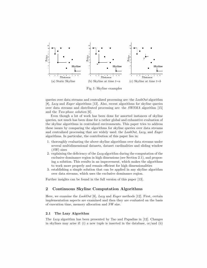
(a) Static Skyline (b) Skyline at time t=a (c) Skyline at time t=b

Fig. 1: Skyline examples

queries over data streams and centralized processing are: the LookOut algorithm[8], Lazy and Eager algorithms [12]. Also, recent algorithms for skyline queriesover data streams and distributed processing are: the SWSMA algorithm [15]and the Two-phase solution [6].

Even though a lot of work has been done for assorted instances of skylinequeries, not much has been done for a rather global and exhaustive evaluation ofthe skyline algorithms in centralized environments. This paper tries to addressthese issues by comparing the algorithms for skyline queries over data streamsand centralized processing that are widely used: the LookOut, Lazy, and Eageralgorithms. In particular, the contribution of this paper lies in:

1. thoroughly evaluating the above skyline algorithms over data streams underseveral multidimensional datasets, dataset cardinalities and sliding window(SW) sizes

2. explaining the deficiency of the Lazy algorithm during the computation of theexclusive dominance region in high dimensions (see Section 2.1), and propos-ing a solution. This results in an improvement, which makes the algorithmsto work more properly and remain efficient for high dimensionalities

3. establishing a simple solution that can be applied in any skyline algorithmover data streams, which uses the exclusive dominance region.

Further insights can be found in the full version of this paper [13].

2 Continuous Skyline Computation Algorithms

Here, we examine the LookOut [8], Lazy and Eager methods [12]. First, certainimplementation aspects are examined and then they are evaluated on the basisof execution time, memory allocation and SW size.

2.1 The Lazy Algorithm

The Lazy algorithm has been presented by Tao and Papadias in [12]. Changesin skylines may arise if: (i) a new tuple is inserted in the database, or/and (ii)

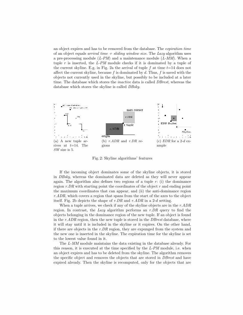
an object expires and has to be removed from the database. The expiration timeof an object equals arrival time + sliding window size. The Lazy algorithm usesa pre-processing module (L-PM) and a maintenance module (L-MM). When atuple r is inserted, the L-PM module checks if it is dominated by a tuple ofthe current skyline. E.g. in Fig. 2a the arrival of tuple f at time t=14 does notaffect the current skyline, because f is dominated by d. Thus, f is saved with theobjects not currently used in the skyline, but possibly to be included at a latertime. The database which stores the inactive data is called DBrest, whereas thedatabase which stores the skyline is called DBsky.

(a) A new tuple ar-rives at t=14. TheSW size is 5.

(b) r.ADR and r.DR re-gions

(c) EDR for a 2-d ex-ample

Fig. 2: Skyline algorithms’ features

If the incoming object dominates some of the skyline objects, it is storedin DBsky, whereas the dominated data are deleted as they will never appearagain. The algorithm also defines two regions of a tuple r: (i) the dominanceregion r.DR with starting point the coordinates of the object r and ending pointthe maximum coordinates that can appear, and (ii) the anti-dominance regionr.ADR, which covers a region that spans from the start of the axes to the objectitself. Fig. 2b depicts the shape of r.DR and r.ADR in a 2-d setting.

When a tuple arrives, we check if any of the skyline objects are in the r.ADRregion. In contrast, the Lazy algorithm performs an r.DR query to find theobjects belonging in the dominance region of the new tuple. If an object is foundin the r.ADR region, then the new tuple is stored in the DBrest database, whereit will stay until it is included in the skyline or it expires. On the other hand,if there are objects in the r.DR region, they are expunged from the system andthe new one is inserted in the skyline. The expiration time for the skyline is setto the lowest value found in it.

The L-MM module maintains the data existing in the database already. Forthis reason, it is executed at the time specified by the L-PM module, i.e. whenan object expires and has to be deleted from the skyline. The algorithm removesthe specific object and removes the objects that are stored in DBrest and haveexpired already. Then the skyline is recomputed, only for the objects that are

dominated exclusively by a tuple r, which is about to be deleted. In Fig. 2c theExclusive Dominance Region (EDR) for a 2-d example is depicted. Then, thealgorithm defines the next execution time for the L-MM module, namely thetime an object will be deleted from the system.

2.2 The Eager Algorithm

The Lazy algorithm has some disadvantages: it stores obsolete data, i.e. tuplesthat will never be used in the skyline. This motivated its authors to considerthe Eager algorithm [12], which aims to: (i) lower the memory consumption bykeeping only the tuples that are or will be part of the skyline, and (ii) lowerthe cost of the maintenance module, in this case the E-MM. Eager achievesthese two goals by doing more in the pre-processing module E-PM, where theinfluence time is computed to predict at arrival time, if a tuple will be includedin a future skyline. If there is no such time, the object can safely be discarded.Eager uses an Event List, in which the events are sorted ascending based onthe time of their respective events. Such events are the expiration of an object,or the transfer from the database to the skyline. Each tuple that is not partof the skyline but will be in the future, is marked and transferred to it at theproper time. Specifically in the E-PM module, for each incoming tuple, a queryfinds the tuples that are dominated by the incoming one. These tuples are thenremoved from the system. The new r tuple is inserted in the database and theinfluence time is computed by finding all the skyline objects that are in ther.ADR region and then keeping the greatest expiry time. At that time point,tuple r will be transferred from the database to the skyline. If the computedinfluence time equals the arrival time, then the tuple is directly inserted in theskyline, whereas in the event list is marked with an EX value. Otherwise, it isstored in the database with the an EL value.

When the time for an event comes, the E-MM method is executed. Thismethod is less complicated than its respective in Lazy algorithm, because moreprocessing is being done in the E-PM module. Thus, if the next event in thelist is marked as EX, then the tuple is simply removed. Otherwise, the tuple isincluded in the skyline and a new event is stored in the event list to indicate thetuple expiry time.

3 The LookOut Algorithm

The LookOut algorithm connects each object with a time interval for which it isvalid [8]. This time interval consists of the arrival time and the expiry time. Theskyline can change in two occasions: (i) some skyline data are about to expire,and (ii) new data are inserted in the database.

The LookOut algorithm takes advantage of two important observations inhierarchical spatial indexes, e.g. R-trees [3] and quadtrees [10]: (i) if point pdominates all corners of a node n, then p dominates all the objects of the nodeand its children, and (ii) if all corners of a node n dominate a point p, then all

objects and its children dominate that point. With these observations pruningof nodes is possible and rejection of new objects is faster. Each new object isinserted in the database and then the expiry time is stored in a min heap. Theobject is checked if it belongs to the skyline by an isSkyline algorithm. If anobject must be removed, then all candidates that may replace it in the skylineare computed by a MINI algorithm. Final insertion is done only if isSkylinereturns true.

isSkyline uses BFS, i.e. nodes with the lowest distance are inserted first inthe heap. When expanding a node, if the lower left corner does not dominate thearriving tuple, it is rejected. If the upper right corner of a child dominates thenew tuple, then the algorithm terminates with negative output and the tupleis not inserted in the skyline. If the node is a leaf, the tuple is compared fordomination against all tuples of the leaf. If there is such a leaf, the incomingobject is not inserted in the skyline, otherwise it is.

The MINI algorithm uses also BFS and a min heap for the distance from theorigin to the point coordinates. An object that is about to be deleted is passed asan argument and returns the objects that are dominated by it. In addition, theseobjects are checked before insertion for domination by others that have alreadybeen inserted. According to the isSkyline algorithm, if the upper right corneris dominated by the object that is about to be deleted, the node is rejected,otherwise if it is an internal dominated node, it is inserted in the heap. If thenode currently checked is a leaf, then the local skyline is computed and stored.

4 Experimentation and Evaluation

4.1 Methodology

For a thorough experimentation we rely on well selected datasets. For this reasonthree data types have been created, by using the generator of [1], and tested: (i)correlated data, (ii) anti-correlated data, and (iii) independent data. As spatialindex we use R-trees [3], [7], which store objects in nodes dynamically generatedat insertion time. Every node represents a Minimum Bounding Rectangle (MBR)and is created by using the coordinates of the lower-left and upper-right MBRcorners. This way, during traversal it is possible to prune insignificant nodes.

The Branch-and-Bound Skyline (BBS) algorithm was used for all three algo-rithms [9]. The BBS algorithm traverses the tree and expands each node, storingin ascending order the distances from the axes origin. In each iteration, the nodewith the lowest distance is expanded or discarded. If the node is dominated bythe existing skyline, it is rejected, otherwise kept. When the algorithm finds aleaf, it inserts the data in the skyline, because they already have been checked.

4.2 Improvement of Lazy Algorithm

According to the Lazy algorithm, the EDR must be computed for L-MM algo-rithm to work. This is easily achieved in 2-d datasets. An ascending ordered

array is needed for each skyline dimension. Then finding the next value, afterthe point that is about to be deleted, creates a tuple for the upper-right cornerof the EDR. The EDR region is computed by using the coordinates of the pointto be deleted with the coordinates of the upper-right corner. This is depicted inFig. 3.

Fig. 3: Computing a 2-d EDR

However, in more than 2 dimensions the shape of the EDR becomes com-plicated and its computation hard or even impossible [14]. The authors of [12]do not clarify how the EDRs were computed and if the datasets allowed thecreation of EDRs that could be computed easily as in 2-d datasets.

To correct these problems we made an improvement in the Lazy algorithm byreplacing the EDR computation of a point with its dominance region (DR) fordimensions higher than 2. With this technique Lazy can return correct resultsfor all dimensions and remain efficient.

4.3 Time Performance

Several tests were conducted by varying the dimensionality and the SW sizeon an Intel Core 2 Duo P8600, with 3GB RAM, 5400 RPM HDD and 64-bitWindows OS. In all tests the Eager algorithm prevails, as tuples are checkedonly once at arrival time if they belong in the skyline. In addition, the Eageralgorithm has a linear scaling in all dimensions and SW sizes. The Lazy algorithmhas similar performance for 2-d datasets; however, its performance is heavilycompromised in higher dimensions. This is due to the dominance region in morethan 2 dimensions. In this case, the search region is far greater than in the EDRregion and, thus, the number of tuples to be checked is much greater as well.

The LookOut algorithm is worse in all cases. For small SW sizes the differenceis comparable, but for sizes greater than some hundreds, the execution timeincreases dramatically. One reason is the MINI algorithm. For mini-skyline tobe computed, all tuples that have not been pruned in the expansion phase, arepotential insertions in the skyline and have to be checked. When the SW sizegets larger, more tuples are possible members of the skyline and must be checkedwith each other. Another issue of the LookOut algorithm is after the execution ofthe MINI, when the isSkyline has to be executed, so that the potential membersare sorted and accordingly rejected or inserted in the skyline.

In addition, all three algorithms seem to perform better in correlated data.This is probably due to better MBR creation and more effective pruning, whichresults in faster tree traversals. Tables 1-3 contain the experimental results.

Dimensions 2-d 4-d 6-d

SW size Lazy Eager LookOut Lazy Eager LookOut Lazy Eager LookOut

100 16.05 6.17 24.32 14.19 6.49 102.87 29.91 7.09 184.71

1K 7.26 11.01 63.11 122.89 13.29 411.80 139.78 12.49 1264.03

10K 13.09 16.41 189.27 1249.90 30.09 1819.39 11415.70 27.59 9969.60

Table 1: Execution time (in seconds), for anti-correlated data

Dimensions 2-d 4-d 6-d

SW size Lazy Eager LookOut Lazy Eager LookOut Lazy Eager LookOut

100 5.06 5.44 21.56 14.18 7.56 113.59 25.24 6.72 162.12

1K 6.52 10.89 52.75 123.09 12.93 428.73 137.27 11.79 1231.35

10K 13.99 16.18 184.63 1776.30 31.15 1773.00 12522.34 47.05 12920.20

Table 2: Execution time (in seconds), for independent data

Dimensions 2-d 4-d 6-d

SW size Lazy Eager LookOut Lazy Eager LookOut Lazy Eager LookOut

100 5.28 4.74 18.45 12.20 5.76 86.32 17.96 6.00 151.75

1K 5.48 9.03 45.29 103.70 11.62 323.01 117.59 10.93 1083.14

10K 7.12 14.85 166.96 1118.71 28.10 1624.72 11814.40 38.53 12492.90

Table 3: Execution time (in seconds), for correlated data

4.4 Memory Consumption

Authors of [12] state that Eager algorithm was developed to consume less mem-ory than Lazy. This is verified by the experiments, because even in the 6-ddatasets and the largest SW, the algorithm consumes less than 10Mb of memoryas shown in Table 4.

On the other hand, the Lazy and the LookOut algorithms have higher mem-ory consumption, since they exceed in some cases dozens of Mb even in 2-ddatasets. The Lazy algorithm displays fluctuations in the memory allocation atsmall SW sizes, but its memory consumption is linear in greater sizes. The Look-Out algorithm has linear consumption, but when the SW size is 1M the memoryconsumption reaches and surpasses 50Mb (see Table 5).

5 Conclusions

This paper examines three skyline algorithms and compares their performance.Experiments established the fact that the dimensionality and the SW size are themain factors that affect the performance and the effectiveness of an algorithm,

which is not clearly visible in small datasets. Also, the dominance region wasused in the Lazy algorithm for the computation of the skyline, as the ExclusiveDominance Region is sometimes impossible to be computed in higher dimensions.

SW size 2-d 4-d 6-d

100 0.5 0.5 0.51K 0.5 0.6 0.610K 0.5 0.8 1.2100K 0.6 1.2 2.91M 0.6 1.2 6.9

Table 4: Memory consumption (in Mb)of Eager algorithms for 2-, 4-, 6-d data

SW size Lazy LookOut

100 10 0.51K 2.9 0.610K 2.3 1.4100K 7.5 8.51M 67.5 58.0

Table 5: Memory consumption (in Mb)of LookOut and Lazy for 2-d data

References

1. Borzsonyi, S., Kossmann, D., Stocker, K.: The skyline operator. In: Proc. ICDE.pp. 421–430 (2001)

2. Chomicki, J., Godfrey, P., Gryz, J., Liang, D.: Skyline with presorting. In: Proc.ICDE. pp. 717–719 (2003)

3. Guttman, A.: R-trees: A dynamic index structure for spatial searching. In: Proc.SIGMOD. pp. 47–57 (1984)

4. Kossmann, D., Ramsak, F., Rost, S.: Shooting stars in the sky: an online algorithmfor skyline queries. In: Proc. VLDB. pp. 275–286 (2002)

5. Li, X., Wang, Y., Li, X., Wang, Y.: Parallel skyline queries over uncertain datastreams in cloud computing environments. International Journal on Web & GridServices 10(1), 24–53 (2014)

6. Lu, H., Zhou, Y., Haustad, J.: Efficient and scalable continuous skyline monitoringin two-tier streaming settings. Information Systems 38(1), 68–81 (2013)

7. Manolopoulos, Y., Nanopoulos, A., Papadopoulos, A., Theodoridis, Y.: R-Trees:Theory and Applications. Springer (2005)

8. Morse, M., Patel, J., Grosky, W.: Efficient continuous skyline computation. Infor-mation Sciences 177(17), 3411–3437 (2007)

9. Papadias, D., Tao, Y., Fu, G., Seeger, B.: An optimal and progressive algorithmfor skyline queries. In: Proc. SIGMOD. pp. 467–478 (2003)

10. Samet, H.: The quadtree and related hierarchical data structures. ACM ComputingSurveys 16(2), 187–260 (1984)

11. Tan, K.L., Eng, P.K., Ooi, B.: Efficient progressive skyline computation. In: Proc.VLDB. pp. 301–310 (2001)

12. Tao, Y., Papadias, D.: Maintaining sliding window skylines on data streams. TKDE18(3), 377–391 (2006)

13. Tzanakas, A., Tiakas, E., Manolopoulos, Y.: Revisited skyline query algorithms onstreams of multidimensional data. Tech. rep. (2016), http://delab.csd.auth.gr

14. Wu, P., Agrawal, D., Egecioglu, O., El Abbadi, A.: DeltaSky: optimal maintenanceof skyline deletions without exclusive dominance region generation. In: Proc. ICDE.pp. 486–495 (2007)

15. Xin, J., Wang, G., Chen, L., Zhang, X., Wang, Z.: Continuously maintaining slidingwindow skylines in a sensor network. In: Proc. DASFAA. pp. 509–521 (2007)