skis & bikes - investresolve · skis and bikes: the untold story of diversification 2 reolve...

Adam Butler, CFA

Michael Philbrick

Rodrigo Gordillo

SKIS & BIKESTHE UNTOLD STORY OF DIVERSFICATION

Skis and Bikes: The Untold Story of Diversification

2 ReSolve Asset Management

The most fundamental principle of investing is diversification. But in our experience, few investors

understand what diversification means. Sure, investors typically understand that diversification

means “don’t put all your eggs in one basket”. Some also understand that diversification is about

owning a combination of investments that zig and zag at different times. But when we probe a little

deeper, it seems many investors are still confused about how diversification works in practice. They

wonder, “If I’m buying something that makes money when the other is losing money, doesn’t that

just give me a zero return?”

In this report we hope to clear up some of the more nuanced complexities of diversification with

a few simple examples.



Store5

4

3

2

1

0

Bikes Skis

Dec Dec Jun Jun JunDec Dec Dec Dec

SECTION 1: SKIS AND BIKES

In most parts of Canada we have very distinct seasons. Some months of the year are temperate

and relatively dry, while other months are cold and snowy. As a result, most Canadian towns of any

size have stores that sell skis and bikes.

Of course, they don’t inventory both skis and bikes at the same time. Rather, in the spring they

sell off all their ski related inventory and set out their bike gear, and in the fall they clear out the bike

gear to make room for skis. Pretty creative, right? Let’s observe a simplified example of bike sales

and ski sales over several years.

Figure 1. Sales of skis and bikes

Source: ReSolve Asset Management. For illustrative purposes only.

As winter approaches, ski sales accelerate while bike sales drop off. As summer approaches

people stop buying skis, but ramp up their purchases of bikes. One line of business is thriving while

the other is flat. In some years, winter might come late and produce very little snow, stifling ski sales.



But the subsequent spring might be warm and dry, and encourage bumper bike sales. This is the

nature of diversification.

This same effect plays out in markets. Economic news that is good for one type of investment

is often bad news for another. In fact, the hallmark of a diversified portfolio is the observation that

one or more investments is disappointing you most of the time. A portfolio that consists of assets

that all produce gains at similar times for similar reasons will probably produce their worst losses

at the same time too.

SECTION 2: WELL-EXECUTED DIVERSIFICATION IS INDISTINGUISHABLE FROM MAGIC

The skis and bikes example above shows how deriving cash-flows from two independently

profitable businesses, which produce returns at different times, reduces the variability of cash-

flows throughout the year. This is helpful because it makes it easier for the business owner to

manage investments in the business, and stabilizes the owner’s income. In other words, diversifying

across two return sources – skis and bikes – lowers the overall risk of the business. Let’s examine

why this is so important.

If the business owner simply wanted to reduce his risk, he could have abandoned the business

altogether, and kept his savings in safe bonds or cash. But the business owner needs to take some

risks to earn a higher income. Both the ski business and the bike business are risky enterprises

on their own, with highly fickle cash-flows. Either one might have been too risky for the shop

owner to earn a stable income. But when the businesses are combined, the resulting ‘portfolio’ of

businesses is much more stable.

The skis and bikes example extends quite intuitively to the domain of investment portfolios. In

investing, it is a simple thing to build a low-risk portfolio by holding lower risk assets, like short-

term government bonds. Unfortunately, this portfolio would not be expected to generate much in



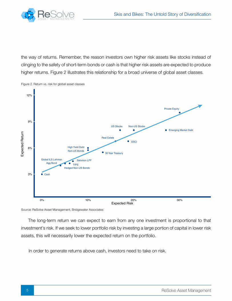
the way of returns. Remember, the reason investors own higher risk assets like stocks instead of

clinging to the safety of short-term bonds or cash is that higher risk assets are expected to produce

higher returns. Figure 2 illustrates this relationship for a broad universe of global asset classes.

Figure 2. Return vs. risk for global asset classes

Source: ReSolve Asset Management, Bridgewater Associates

The long-term return we can expect to earn from any one investment is proportional to that

investment’s risk. If we seek to lower portfolio risk by investing a large portion of capital in lower risk

assets, this will necessarily lower the expected return on the portfolio.

In order to generate returns above cash, investors need to take on risk.



The magic of diversification is that it allows investors to keep more of their money

invested in higher risk assets, with commensurately higher expected returns, while lowering

the overall risk of the portfolio.

Section 3 below illustrates this concept with a theoretical example, while Section 4 provides

evidence with real asset classes. Section 5 illustrates the power of diversification to produce stable

returns across most investment environments.

SECTION 3: DIVERSIFICATION IN THEORY

The central advantage of diversification is that it allows investors to hold many risky assets,

while maintaining a tolerable level of portfolio risk. But many investors express confusion about

how two investments can both be expected to rise in value, even while they are uncorrelated. After

all, if they are uncorrelated, shouldn’t we expect them to move in different directions? The skis and

bikes example offers some perspective on this apparent contradiction. The revenues accumulated

from both skis and bikes are rising over time. But they are rising at precisely opposite times. As a

result, the shop owner can even out his revenue streams across the different seasons of the year.

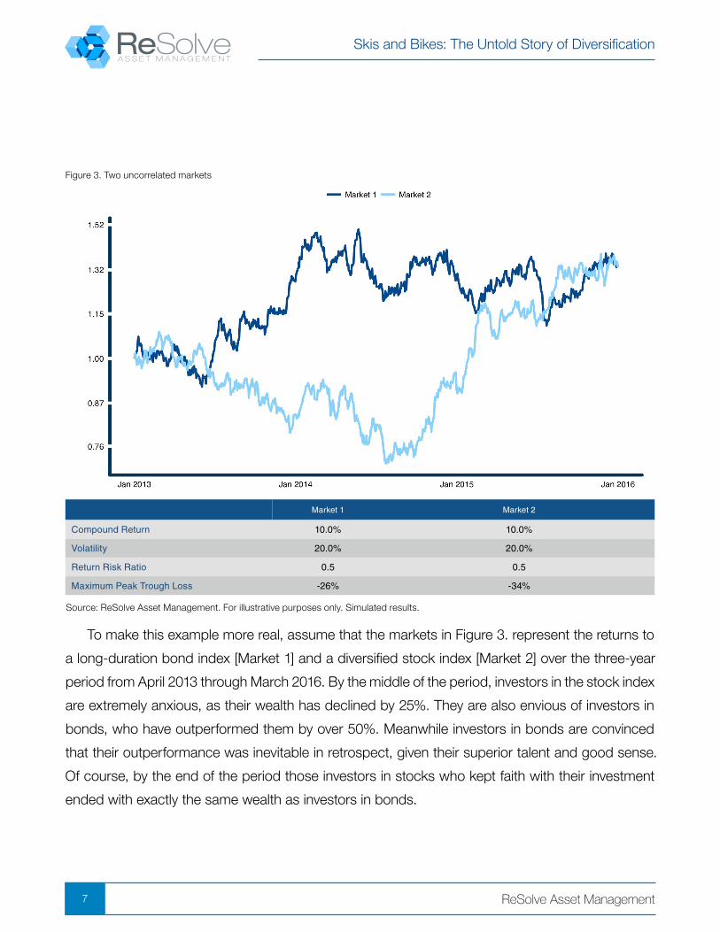
Now let’s apply this same phenomenon to two investments. In Figure 3. below both Market 1

and Market 2 grow at the same rate of 10% per year for three years. We know this is true because

the assets’ prices begin and end in the same place. In addition, the assets fluctuate the exact same

average amount from day to day – that is, they have the same “volatility”. However, Market 1 and

Market 2 take a very different path to the same final destination. Market 1 shoots up early on but

then returns flatten out and become choppy. Market 2 endures a steady decline over the first half

of the period, but then shoots higher. Market 1 inflicts a 26% maximum peak-to-trough loss while

Market 2 forces investors to endure an even steeper decline of 34% before recovering.



Market 1 Market 2

Compound Return 10.0% 10.0%

Volatility 20.0% 20.0%

Return Risk Ratio 0.5 0.5

Maximum Peak Trough Loss -26% -34%

Figure 3. Two uncorrelated markets

To make this example more real, assume that the markets in Figure 3. represent the returns to

a long-duration bond index [Market 1] and a diversified stock index [Market 2] over the three-year

period from April 2013 through March 2016. By the middle of the period, investors in the stock index

are extremely anxious, as their wealth has declined by 25%. They are also envious of investors in

bonds, who have outperformed them by over 50%. Meanwhile investors in bonds are convinced

that their outperformance was inevitable in retrospect, given their superior talent and good sense.

Of course, by the end of the period those investors in stocks who kept faith with their investment

ended with exactly the same wealth as investors in bonds.

Source: ReSolve Asset Management. For illustrative purposes only. Simulated results.



Remember that both Market 1 and Market 2 have the same expected average returns over the

long-term. However, they move in different directions at different times for different reasons. In other

words, they are uncorrelated. If we expect the same average outcome from both markets, and they

are different, then we should take advantage of the opportunity for diversification. Consider the

experience of an investor that places half of her capital in Market 1 and half in Market 2 over the

same period.

Figure 4. Combining two uncorrelated markets

Market 1 Market 2 Combo

Compound Return 10.0% 10.0% 10.0%

Volatility 20.0% 20.0% 13.7%

Return Risk Ratio 0.5 0.5 0.73

Maximum Peak Trough Loss -26% -34% -18%




When we examine the full three-year experience of a diversified investor relative to investors

with concentrated investments in just one market, it’s clear that diversification produces a gentler

ride. While the diversified portfolio produced the same return, it did so with about 1/3 less volatility.

Even better, because the declines in the two markets occurred at different times, the diversified

portfolio achieved its returns with a 40% smaller peak-to-trough loss than that endured by investors

in either of the individual markets.

However, while it’s clear with the benefit of perfect hindsight that diversified investors were

better off over the entire period, it’s illustrative to revisit how each investor might have felt half-way

through. At that time, investors who chose to diversify were probably regretting their decision, as

Market 1 had produced about 25% in extra returns. They were wishing that they had never even

heard of Market 2! Only after the completion of the period, once Market 1 experienced its own 26%

decline, would diversified investors finally have felt vindicated.

What makes investing so incredibly challenging is that we can’t know for sure in advance

whether two investments will produce the same returns, or whether one investment will produce

higher returns than another. And even if there is a high degree of confidence that one investment

will beat another in the long term, there is no guarantee that returns will converge over a time

horizon that investors can live with. For example, over the two decades from 1981 through 2001,

safe U.S. government Treasury bonds produced higher returns than stocks, without inflicting the

pain and anxiety of two major bear markets1.

Ironically, this uncertainty about the true average return is actually a good thing. If investors

knew the true average return of their investments in advance, it’s likely that these investments would

attract a lot more capital. This would drive the price of the investments so high that future investors

would necessarily earn a much lower return.

1 Source: Global Financial Data



As a thought experiment, it’s interesting to see how introducing more uncorrelated investments

can make the experience even smoother. For example, in the event an investor could construct

five uncorrelated investments with the same 10% expected compound return and 20% volatility,

an equally weighted portfolio would have the same return, but less than half the volatility, of any

of the individual investments. Even better, while the average peak-to-trough loss of each individual

investment is close to 30%, the peak-to-trough loss of the portfolio is well under 10%.

Figure 5. Combining 5 uncorrelated sources of return

Investment 1 Investment 2 Investment 3 Investment 4 Investment 5 Combo

Compound Return 10.0% 10.0% 10.0% 10.0% 10.0% 10.0%

Volatility 20.0% 20.0% 20.0% 20.0% 20.0% 8.7%

Return Risk Ratio 0.5 0.5 0.5 0.5 0.5 1.14

Maximum Peak Trough Loss -26% -34% -30% -27% -25% -7.2%




As you can see, the “Holy Grail” of diversification is the ability to introduce streams of

investment returns from many diverse sources. The emphasis here is on the word ‘diverse’, as it

is unhelpful, from a diversification standpoint, to add many investments that are highly correlated.

However, the diversification advantage from adding many uncorrelated investments to a portfolio is

indistinguishable from magic.

SECTION 4: DIVERSIFICATION IN PRACTICE

We’ve seen that by combining investments with uncorrelated return streams, we can create a

portfolio that preserves returns while dramatically reducing risk. This is interesting in theory, but it

prompts the question: how can we make diversification work for us in practice?

There are two parts to this answer. The first part addresses how to fit together assets with

different risk profiles. The second part deals with finding truly uncorrelated investments. It turns out

this is harder than people think, and most investors get it wrong.

STEP ONE: BALANCE

Diversification is about balance. Unfortunately, while many investors own products that are

labeled “balanced”, the portfolios underlying those products are anything but. The imbalance

occurs because the assets in the portfolio have wildly different risk profiles. As Figure 5 shows,

when you hold an equal portion of stocks and bonds in a portfolio, the portfolio is completely

dominated by stock risk, because stocks are so much more volatile than bonds.



Figure 6. A portfolio equally divided between U.S. stocks and Treasuries is dominated by stock risk

Source: ReSolve Asset Management. Data from CSI.

This large imbalance is not just a theoretical curiosity. It has a very real economic impact

on portfolios. Remember, portfolios should be engineered to be resilient to all major economic

environments. But stocks are designed to produce positive returns only during periods of sustained

positive growth shocks, with benign inflation and abundant liquidity conditions.

When these conditions are present, the portfolio does well. However, when growth plummets

unexpectedly, or inflation spirals out of control, the true personality of this portfolio reveals itself.

Consider the performance of this 50/50 portfolio of U.S. stocks and high-grade bonds during the

global growth shock in 2008-2009 (Figure 7.).



Figure 7. Equal weight U.S. stocks and high grade corporate bonds: Daily inflation adjusted total returns, Oct 2007 – Mar 2009, log-scale


The Global Financial Crisis of 2008 inflicted a 33% peak-to-trough loss on U.S. investors

holding equal weight portfolios of high grade bonds and stocks. Investors outside the U.S. fared

approximately the same with a similar portfolio configuration. This despite the fact that the bond

portion of the portfolio held its value throughout.

Another way to observe the fact that an equally weighted portfolio of stocks and bonds is

just a diluted stock portfolio is to examine the correlation between this portfolio and stocks over

time. From Figure 7 it’s obvious that despite having 50% in bonds, the portfolio is almost perfectly

correlated with stocks most of the time. The average correlation is .91, and the portfolio’s correlation

with stocks has never dropped below 0.8 since 1993.



Figure 8. Rolling 3-year correlation between U.S. stocks and equally weighted portfolio of stocks and bonds, 1993-2017


It’s clear that traditional “balanced” portfolios are not balanced at all. The much higher volatility

of stocks relative to bonds means that bonds have no opportunity to express their diversification

benefits. This is no trivial matter because, as we’ll see in the next section, bonds can provide

substantial diversification with the right amount of balance.

STEP TWO: DIVERSITY

Unfortunately, most investors seek diversification in the wrong places. For example, many

investors perceive that holding many different stocks or stock mutual funds in a portfolio will

produce strong diversification benefits. This is like seeking greater diversification and lower risk

from buying several ski stores across Canada. Sure, different parts of Canada may have better or

worse ski seasons in different years, but summer months are still going to be tough.



It works the same way for stocks and stock mutual funds, because all of the stocks in a market

are influenced by the same force: economic growth expectations. Stocks will all fall together if

economic growth is weaker than expected, and vice versa. This is even true for stocks in different

countries, because economic growth for individual countries is often tied to general global economic

trends.

To illustrate this point, let’s examine whether we can achieve meaningful diversification by

combining the 14 largest global stock markets in the MSCI All-Cap World Index (ACWI). The ACWI

is constructed to represent over 99% of total global equity market capitalization, and the 14 markets

that we’ve chosen represent over 75%. (Note: we excluded China due to lack of long-term index

data). Figure 6 shows the annualized volatility over the 26-year period ending October 31, 2016 for

each index (in USD)2.

How can we measure the available diversification opportunity? A simple method would be to

observe the ratio between the average of the volatilities across each individual market, and the

volatility of the equally weighted portfolio of the same constituents. We’ll call this the “diversification

ratio”. The average of the individual volatilities does not account for the diversification benefit,

while the volatility of the equally weighted portfolio does, so the ratio measures the risk reduction

advantage of diversification.

From Figure 9, we see that the average of individual market volatilities is 26.4% (red bar), while

the volatility of the equally weighted portfolio is 19.8% (green bar). Thus, the diversification ratio

is 26.4%/19.8% = 1.33. In other words, we achieve a 33% diversification advantage from dividing

capital equally among 15 of the largest global equity market indexes.

2 Where daily index histories did not extend to 1991 we calculated from inception. Portfolio volatility was calculated from pairwise complete covariances.



Figure 9. Annualized volatility of ACWI constituents, 1991 - 2017

Source: ReSolve Asset Management. Data from CSI and MSCI.

You may be surprised to learn that earning a 33% risk-adjusted performance advantage from

diversification is relatively thin gruel. Remember that diversification benefits are a function of low

correlation between the assets in the portfolio. However, over the past 26 years the average

correlation between these global equity markets is about 0.6. Worse, since the proliferation of index

products has made it easy to invest in international markets, correlations have steadily increased.

Figure 9 describes the rolling average annual pairwise correlations between these markets from

1999 through 2016, and the trend of these correlations. High correlations between global equity

markets might be here to stay, which further dilutes the diversification opportunities within the

global equity asset class.



Figure 10. Rolling average annual pairwise correlations of ACWI constituent indexes

Source: ReSolve Asset Management. Data from CSI and MSCI.

While investors focused on global stock markets are likely to experience diminishing returns

on diversification, other opportunities for diversification abound. However, investors seeking

diversification must be willing to look further afield.

Remember, investment environments are generally defined by unexpected changes to inflation

and growth expectations. Figure 10 divides economic environments along these two dimensions to

create four distinct economic states of the world. Diverse global asset classes are embedded in the

quadrants in which they would be fundamentally expected to perform well. Assets near the middle

have low sensitivity to the corresponding economic dynamics, while those near the edge are highly

sensitive and volatile. You can see that stocks would be expected to flourish during periods of

unexpectedly strong growth, while other assets like government bonds, TIPs, commodities, REITs

and gold are designed to produce their best returns in very different economic periods.



Figure 11. Global asset class sensitivities to growth and inflation

Source: ReSolve Asset Management.

Since there are assets available to investors that can be expected to produce positive returns in

any environment, the investment universe in Figure 10 is truly diversified. Let’s extend our analysis

of diversification benefits using this more diverse group of assets. Specifically, consider a universe

of global assets consisting of U.S., European, Asian and emerging market stock indexes; U.S. and

international real estate securities (REITs); gold; commodities; Treasury Inflation Protected Securities

(TIPs); U.S. government bonds (Treasuries), foreign bonds, and; USD denominated emerging market



bonds. Figure 12. quantifies the annualized volatility of each of these asset class indexes over the

period 1991 through 20163.

3 Where daily index histories did not extend to 1991 we calculated from inception. Portfolio volatility was calculated from pairwise complete covariances.

Figure 12. Annualized volatility of global asset classes

Source: ReSolve Asset Management. Data from CSI and Bloomberg.

Recall from Figure 9 that, because global equity markets are highly correlated with one another,

investors accrue a rather small (33%) advantage from holding them all together in a portfolio. In

contrast, it’s clear from Figure 10 that our diversified universe provides much larger benefits. The

average of individual asset class volatilities is 17.1% (red bar), while the volatility of the equally

weighted portfolio is 9.9% (green bar). Thus, the diversification ratio is 19.8%/12% = 1.73. In other

words, we achieve a 73% diversification advantage from dividing capital equally among 13 major

global asset classes.



Even better, there is no reason to believe that this diversification benefit from investing in diverse

global asset classes will go away anytime soon. Figure 13 clearly shows that the average annual

pairwise correlations between these diverse asset classes have been persistently low, averaging

0.25 compared to the average 0.6 correlations across global equity markets. And, in contrast

to what we observe across global equity markets, the trend does not appear to be increasing

materially over time.

Figure 13. Rolling average annual pairwise correlations of global asset classes.

Source: ReSolve Asset Management. Data from CSI and Bloomberg.

The lesson from this section is that diversification has very practical benefits, but only for

investors who can think more broadly about the world’s many sources of returns. Investors who

are uncomfortable investing outside their borders, or in unfamiliar asset classes, will incur large

opportunity costs. Either they will own a portfolio that is much more vulnerable to risk in order to

earn the returns they need, or they will own a portfolio that earns a lower return at the level of risk

they can tolerate.



SECTION 5: DIVERSIFICATION FOR STABLE RETURNS IN ALL ENVI-RONMENTS

This paper has made the case that the primary advantage of diversification is that it allows an

investor to hold many risky assets in a portfolio – with commensurately high expected returns – but

with much less risk than would be experienced by holding any single asset on its own. We laid the

foundation for this concept using theoretical uncorrelated return streams, and discovered that it is

possible to combine many risky, but sufficiently uncorrelated assets in a portfolio to dramatically lower

portfolio risk. Finally, we observed the practical benefits of diversification by combining two different

universes of asset classes. We saw that it is challenging to achieve meaningful diversification from

investments across global equity markets, but that there are significant diversification opportunities

from investing in a broader universe of global asset classes.

In this final section, we will explore how to combine all of the concepts discussed so far to

create robust portfolios that are designed to thrive in most economic environments. Specifically,

we will analyse how to use the diverse universe of asset classes described in Figures 11 and 12 to

create maximum balance in a portfolio.

First, let’s revisit the historical personalities of our assets by reflecting on their long-term volatilities,

and their average correlations with all of the other assets. Figure 12 summarized the long-term

average volatilities of major markets. Recall that that Treasury bonds produced just one quarter the

volatility of most risky assets like stocks and commodities over the past 25 years. On the correlation

front, Figure 14 shows that U.S. Treasuries in general have exhibited the lowest correlation with

other assets, followed by gold and commodities. Mostly as a function of currency effects (we use

unhedged bond indexes), foreign bonds are grouped between equities and commodities in terms

of average correlations.



0.03

0.05

0.13

0.15

0.22

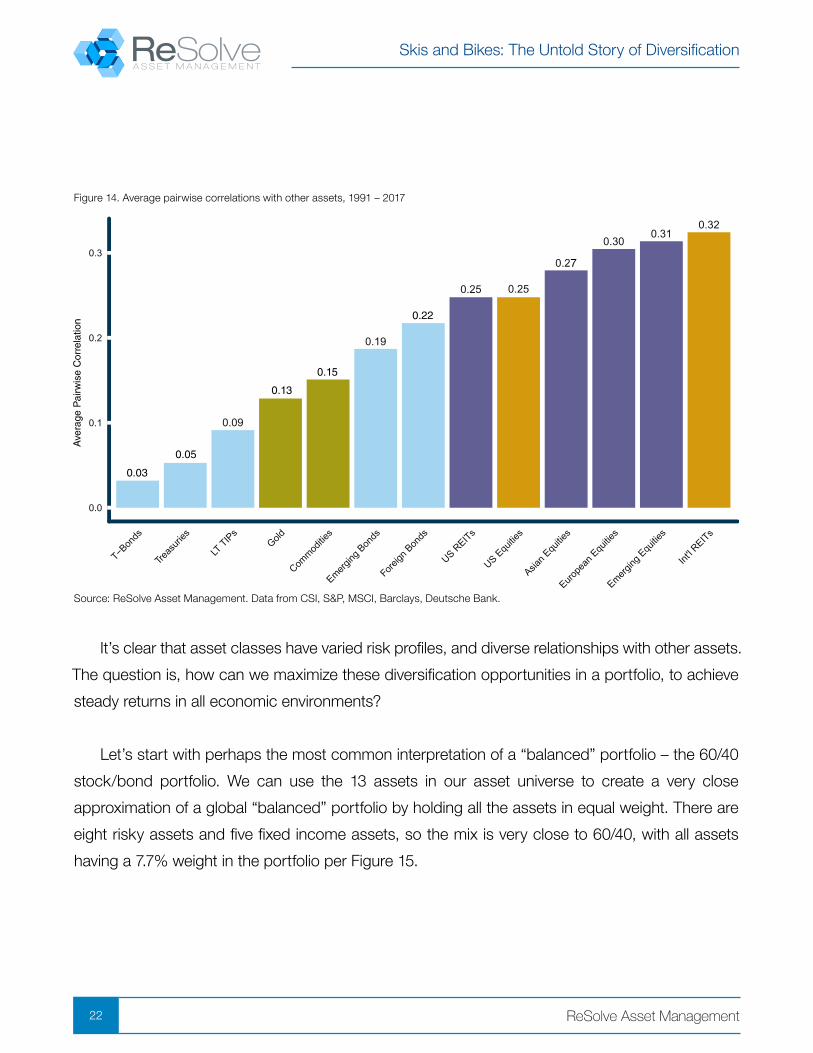
Figure 14. Average pairwise correlations with other assets, 1991 – 2017

Source: ReSolve Asset Management. Data from CSI, S&P, MSCI, Barclays, Deutsche Bank.

It’s clear that asset classes have varied risk profiles, and diverse relationships with other assets.

The question is, how can we maximize these diversification opportunities in a portfolio, to achieve

steady returns in all economic environments?

Let’s start with perhaps the most common interpretation of a “balanced” portfolio – the 60/40

stock/bond portfolio. We can use the 13 assets in our asset universe to create a very close

approximation of a global “balanced” portfolio by holding all the assets in equal weight. There are

eight risky assets and five fixed income assets, so the mix is very close to 60/40, with all assets

having a 7.7% weight in the portfolio per Figure 15.



Figure 15. Equal weight portfolio is a global “balanced” portfolio.


Is this so-called “balanced” portfolio truly balanced? Rather than stopping at a surface level

view of asset weights, let’s examine the portfolio through the lens of the assets’ risk contributions.

Remember, asset classes in this diverse universe have different risk properties.

Some assets are much more volatile and/or highly correlated than others. If we mix volatile

assets with high correlations to other assets alongside stable assets with low correlations, how can

we expect each asset to contribute the same amount of diversification benefits? Per Figure 16, it

turns out that this portfolio is not very balanced at all.

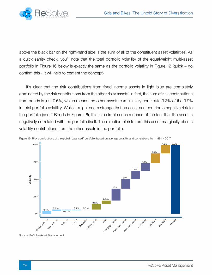
Let’s take a moment to interpret this waterfall chart in Figure 16. Each bar shows the total risk

contribution, in units of volatility, for that asset as a constituent of the portfolio. The portfolio volatility



above the black bar on the right-hand side is the sum of all of the constituent asset volatilities. As

a quick sanity check, you’ll note that the total portfolio volatility of the equalweight multi-asset

portfolio in Figure 16 below is exactly the same as the portfolio volatility in Figure 12 (quick – go

confirm this - it will help to cement the concept).

It’s clear that the risk contributions from fixed income assets in light blue are completely

dominated by the risk contributions from the other risky assets. In fact, the sum of risk contributions

from bonds is just 0.6%, which means the other assets cumulatively contribute 9.3% of the 9.9%

in total portfolio volatility. While it might seem strange that an asset can contribute negative risk to

the portfolio (see T-Bonds in Figure 16), this is a simple consequence of the fact that the asset is

negatively correlated with the portfolio itself. The direction of risk from this asset marginally offsets

volatility contributions from the other assets in the portfolio.

Figure 16. Risk contributions of the global “balanced” portfolio, based on average volatility and correlations from 1991 – 2017




If a traditional “balanced” portfolio isn’t actually balanced, what method can we use to create

a truly balanced portfolio from these diverse assets? Risk Parity is the concept of constructing a

portfolio so that each asset has an equal opportunity to express its diverse character. Quantitatively,

this occurs when each asset contributes the same amount of risk to the portfolio. Intuitively, for

assets with different risk profiles to contribute the same amount of risk, a portfolio must hold a

larger weighting in low risk assets, and a smaller weighting in higher risk assets. To maximize

diversity, assets with low correlation to other assets would also receive a higher weighting.

Based on this logic, and with a quick glance at Figures 12 and 14 above, one might expect a

Risk Parity portfolio to have its largest weights in U.S. Treasuries and T-Bonds, since they exhibit

the lowest combination of volatility and correlation relative to the other assets. On the other end of

the spectrum, we might expect emerging market stocks and REITs to have the smallest weights in

the portfolio.

20.2%

11.8%

10.7%

9.8%

9.0%

7.2%

6.0%

5.3%4.4%

4.1%3.2%

4.4%4.0% 100%

Figure 17. Risk contributions of the global “balanced” portfolio, based on average volatility and correlations from 1991 – 2017




Figure 17 shows the true optimal Risk Parity portfolio weights using average volatilities and

correlations from 1991 – 2017. Conveniently, asset weights in the portfolio are broadly aligned with

what we would expect, given their volatility and correlation profiles. Bond type assets are on the

left with the most weight, while risky assets are on the right with less weight. When we view this

portfolio through the lens of risk contributions in Figure 18, we see that all of the assets are now

contributing the same amount of risk to the portfolio. The portfolio is in perfect balance.

Figure 18. Risk contributions for the Global Risk Parity portfolio, based on average volatility and correlations from 1991 – 2017


The truly balanced Global Risk Parity portfolio has significantly less volatility than the global

60/40 portfolio. In fact, the Global Risk Parity portfolio has the same volatility as 10-year Treasury

bonds over the period studied, despite the fact that 80% of the portfolio is comprised of assets

with much higher volatility. Even so, astute readers might wonder what proportion of the reduction

in volatility is simply due to the larger weight in bonds.



We can invoke the “diversification ratio” concept discussed above to disentangle how much

of the reduction in volatility is due to better diversification rather than a higher weighting in bonds.

Recall that the diversification ratio is the ratio of the weighted average volatility of the constituent

assets divided by portfolio volatility. The weighted average volatility of the equally weighted asset

classes was 17.1% (see Figure 10), while the volatility of the equally weighted portfolio was 9.9%,

reflecting a diversification ratio of 1.73. The weighted average volatility of the assets in the Global

Risk Parity portfolio is 13.65%, reflecting a higher weighting in bonds. However, the portfolio volatility

is just 6.5%, so the diversification ratio is 13.65%/6.5% = 2.1.

But so far this is just theory. Let’s face it, few investors care about esoteric objectives like

maximizing the diversification opportunity in a portfolio. Investors care about results.

Specifically, they want to maximize their returns with minimal risk.4 In Figure 19, we examine the

historical character of the global 60/40 portfolio and the Global Risk Parity portfolio over the past

quarter century to see what diversification means in terms of real dollars and cents. Specifically,

let’s use a prudent amount of leverage to scale both strategies to target 10% portfolio volatility. For

simplicity, we assumed investors can borrow (with margin) at the T-bill rate.

4 More accurately, investors want to maximize the probability that they will achieve their financial objectives. However, expected risk-adjusted performance is a good proxy for this probability for investors with reasonable goals.



Figure 19. Global Risk Parity vs. Global 60/40 portfolio, scaled to 10% volatility, 1991 - 2017

This is where theory meets economic reality. The enhanced diversification properties of the

Global Risk Parity portfolio produce higher returns when scaled to the same level of risk as the

Global 60/40 portfolio. In fact, over a quarter century the Global Risk Parity portfolio produces

almost twice as much wealth at the same level of volatility, and with a smaller peak-to-trough loss

(Max Drawdown) along the way.

Statistics Global 60 / 40 Strategic Global Risk Parity

Compound Return 8.32% 10.97%

Volatility 10.0% 10.0%

Sharpe Ratio 0.62 0.86

Maximum Drawdown -40.95% -34.40%

Positive Rolling Yrs 82.00% 82.00%

Growth of $1 $8.14 $15.39




SUMMARY

This paper set out to correct a variety of misconceptions about diversification. Many investors are

fundamentally confused about how two assets can move in different directions without canceling

each other out. In the first section, we described a simple business that sold skis in the winter and

bikes in the summer. The revenues from these two sales channels arrive at different times of the

year, but they both contribute to the bottom line. When combined, the business is able to earn

much more stable cash-flows, perhaps allowing the owner to scale the business more aggressively

for growth.

Diversified investments work the same way in portfolios. As more uncorrelated sources of

return are introduced, portfolios experience lower volatility and smaller peak-to-trough losses. This

is important because investors seek returns by investing in risky assets. Diversification provides the

opportunity to invest in a variety of risky assets – with commensurately high expected returns - but

at a fraction of the total risk that an investor would endure from an investment in any single asset

on its own.

Unfortunately, traditional portfolios get diversification wrong, for two reasons. First, they fail to

account for the fact that asset classes have very different risk profiles. As a result, popular products

like “balanced” funds are completely dominated by the riskier assets in the portfolio, like stocks.

Bonds have no opportunity to provide their diversification “ballast”. That’s why typical “balanced”

portfolios lost between 35% - 40% of their value during the Global Financial Crisis in 2008-2009.

Second, most portfolios fail to invest in diverse assets that thrive in different economic states.

Portfolios that are heavily concentrated in equity risk will only do well during periods of sustained

global growth, benign inflation, and abundant liquidity. Thankfully, with some notable exceptions,

these conditions largely characterize investors’ experience over the past three decades. But such

a long period of conditions favourable to stocks is the exception, not the rule. There have been

three periods over the past century or so, each lasting between 14 and 21 years, where “balanced”

portfolios have produced flat or negative real growth. These periods are real, and they lie somewhere

ahead of us.



Disclaimer

Confidential and proprietary information. The contents hereof may not be reproduced or disseminated without the express written permission of ReSolve Asset Management Inc. (“ReSolve”). ReSolve is registered as an investment fund manager in Ontario and Newfoundland and Labrador, and as a portfolio manager and exempt market dealer in Ontario, Alberta, British Columbia and Newfoundland and Labrador. These materials do not purport to be exhaustive and although the particulars contained herein were obtained from sources ReSolve believes are reliable, ReSolve does not guarantee their accuracy or completeness. The contents hereof does not constitute an offer to sell or a solicitation of interest to purchase any securities or investment advisory services in any jurisdiction in which such offer or solicitation is not authorized.

Forward-Looking Information. The contents hereof may contain “forward-looking information” within the meaning of the Securities Act (Ontario) and equivalent legislation in other provinces and territories. Because such forward-looking information involves risks and uncertainties, actual performance results may differ materially from any expectations, projections or predictions made or implicated in such forward-looking information. Prospective investors are therefore cautioned not to place undue reliance on such forward-looking statements. In addition, in considering any prior performance information contained herein, prospective investors should bear in mind that past results are not necessarily indicative of future results, and there can be no assurance that results comparable to those discussed herein will be achieved. The contents hereof speaks as of the date hereof and neither ReSolve nor any affiliate or representative thereof assumes any obligation to provide subsequent revisions or updates to any historical or forward-looking information contained herein to reflect the occurrence of events and/or changes in circumstances after the date hereof.

General information regarding returns. Performance data prior to August, 2015 reflects the performance of accounts managed by Dundee Securities Ltd., which used the same investment decision makers, processes, objectives and strategies as ReSolve has used since it became registered and commenced operations in August, 2015. Records that document and support this past performance are available upon request. Performance is expressed in CAD, net of applicable management fees. Indicated returns of one year or more are annualized. Past performance is not indicative of future performance.

General information regarding the use of benchmarks. The indices listed have been selected for purposes of comparing performance with widely-known, broad-based benchmarks. Performance may or may not correlate to any of these indices and should not be considered as a proxy for any of these indices. The S&P/TSX Composite Index (Net TR) (“S&P TSX TR”) is the headline index and the principal broad market measure for the Canadian equity markets. The Standard & Poor’s 500 Composite Stock Price Index (“S&P 500”) is a capitalization-weighted index of 500 stocks intended to be a representative sample of leading companies in leading industries within the U.S. economy.

General information regarding hypothetical performance and simulated results. These results are based on simulated or hypothetical performance results that have certain inherent limitations. Unlike the results in an actual performance record, these results do not represent actual trading. Also, because these trades have not actually been executed, these results may have under- or over-compensated for the impact, if any, of certain market factors, such as lack of liquidity. Simulated or hypothetical trading programs in general are also subject to the fact that they are designed with the benefit of hindsight. No representation is being made that any account or fund managed by ReSolve will or is likely to achieve profits or losses similar to those being shown. The results do not include other costs of managing a portfolio (such as custodial fees, legal, auditing, administrative or other professional fees). The contents hereof has not been reviewed or audited by an independent accountant or other independent testing firm. More detailed information regarding the manner in which the charts were calculated is available on request. Any actual fund or account that ReSolve manages will invest in different economic conditions, during periods with different volatility and in different securities than those incorporated in the hypothetical performance charts shown. There is no representation that any fund or account will perform as the hypothetical or other performance charts indicate.

General information regarding the simulation process. The systematic model used historical price data from Exchange Traded Funds (“ETFs”) representing the underlying asset classes in which it trades. Where ETF data was not available in earlier years, direct market data was used to create the trading signals. The hypothetical results shown are based on extensive models and calculations that are available for any potential investor to review before making a decision to invest.

skis & bikes - investresolve · skis and bikes: the untold story of diversification 2 reolve...

Documents