skimming off the topneudc2012/docs/paper_275.pdf · skimming off the top: ... the data span a rapid...

SKIMMING OFF THE TOP: THE UNINTENDED CONSEQUENCESOF MARKET EXPANSION IN THE INDIAN DAIRY INDUSTRY

EMILY BREZA†, ARUN G. CHANDRASEKHAR‡, ASHISH SHENOY§,AND (PRELIMINARY AND INCOMPLETE)

Abstract. The dairy sector in India is orgnaized into village cooperatives, in whichmany indivudals pour milk together for sale to the regional market. In the last decadethe Karnataka Milk Federation, the largest organizer of cooperatives in the Indian stateof Karnataka, has invested heavily in bulk milk chillers (BMCs) that drastically lowerthe time between production and refrigeration. These chillers, by lowering the perceivedrisk of spoilage, both raise the potential returns to high quality milk and increase thetemptation to engage in unsavory practices such as milk dilution. We investigate theeffects of village access to a BMC on the production process through a difference-in-difference approach using village-level data from the district of Kolar. We find thatproduction quantity increases with access to a chiller but average production qualitydecreases, as does the likelihood of being punished for low quality. The results areconsistent with a story in which villagers increase their use of dishonest practices such asdilution after being connected to a BMC because they face less risk of being punished.The effect size varies with village social characteristics, indicating that it is driven inpart by a village’s ability to manipulate the behavior of BMC officers in a manner notpossible at central processing plants. We propose an instrumental variables strategyto supplement our initial analysis and evaluate the impact of BMC access on broadervillage-level economic and political outcomes. The instrument is based on the optimalplacement of chilling centers, as computed by a facility location algorithm inspired bywork in organizational engineering.

JEL Classification Codes: D23, D73, L23, Q13NEUDC Classification: Land and Agriculture - Agriculture

1. Introduction

In India, dairy production is a key source of income for approximately 20% of ruralhouseholds. Each producer operates at an extremely small scale, with the average house-hold owning fewer than three cows. Bringing milk to market and producing value-added

Date: August 2012.We thank Manaswini Rao, Vikas Dimble, Madhumitha Hebbar, and Ben Marx for excellent researchsupport. Also, Abhijit Banerjee, Tavneet Suri, and Esther Duflo for helpful comments and Adam Sacarnyfor coding advice.†Columbia Business School.‡Microsoft Research New England and Stanford University.§Massachusetts Institute of Technology.

1

SKIMMING OFF THE TOP 2

dairy products presents the considerable challenge challenge of maintaining profitablilitydespite high fixed costs.

The dairy sector in India is generally organized into cooperatives, through which milkproducers in a village join a Dairy Cooperative Society (DCS). Milk from each villageDCS is collected and sent to a production facility owned by the cooperative’s umbrellaorganization. In the Indian state of Karnataka, the Karnataka Milk Federation (KMF)comprises of over 2 million members from more than 11,000 DCSs statewide and procuresover 4 million kg of milk per day1.

Villagers in Karnataka have limited ability to produce milk for the general market untilthe KMF decides to charter a new DCS in their village; they are generally otherwiserestricted to selling selling their product exclusively wothon the village. Once a DCS isformed, any milk in excess of local demand is integrated into the broader retail marketfor dairy products. Producers integrated into the state system earn a higher price perliter both due to high demand from urban centers with little local production and due tothe production of value-added goods such as yoghurt and cheese. One key set of factorslimiting market integration is the cost and spoilage risk in transporting unrefrigerated milkfrom villages with poor roads to central processing facilities, which are generally found inlarge towns up to 80 km away.

Over the past decade, the KMF has invested heavily in reducing transportation risksby commissioning and installing thousands of bulk milk chillers (BMCs), providing refrig-eration at the point of village milk collection. One BMC allows access to refrigerationfacilities to up to 4 neighboring villages. Furthermore, the KMF installs the chillers at nocost to the DCSs that benefit, providing a large free public good. We seek to estimate theeffect of building a BMC on the behavior and production habits of individual villagers.

While reducing the spoilage risk borne by each village and increasing the sale price givento each farmer are unequivocally positive developments for any DCS,2 the total value ofconstructing each BMC may not be so clear-cut. Because milk from several villages iscombined at the point of refrigeration, the KMF is unable to provide village-level qualitytesting at the point of delivery, and instead must rely on the measurements taken at thesite of the BMC. These measurements form the basis for each village’s payment, so villagesmay find it difficult to self-monitor. Thus, installing new BMCs has the potential to reduceproduction risks and increase profitability in remote villages, but also introduces incentiveproblems into the dairy production process. In this paper, we seek to understand howproducers respond to the installation of a BMC in or near their village. Namely, what arethe magnitudes and relative importances of these opposing effects?

1http://www.kmfnandini.coop2In general, the per liter price offered to farmers by the KMF is substantially higher than the price availableon the local market.


Using administrative records for more than 1,600 DCSs in 2 districts of Karnataka,we use a differences-in-differences approach to estimate the effects of BMC infrastructureinvestment on milk quality, quantity, and household investment. The 11 years covered bythe data span a rapid period of BMC growth, and we exploit the timing of the actualconstruction across the districts to identify the desired parameters. Furthermore, wedecompose the effects of becoming connected along pre-period quality dimensions. Arebenefits and/or costs accrued to the previously high-quality villages or to low-qualityvillages? In addition to the differences-in-differences model, we outline an instrumentalvariables approach that will be used to corroborate the reduced form results and explorefurther outcomes as data becomes available.

We find that while production quantity improves following the installation of a chiller,there are declines in average quality. The results show that while average quality declines,the number of days per month with low quality penalty payments decreases. While chillersmay reduce uncertainty for producers, this result is consistent with the effects of reducedmonitoring, leading to perverse behavior by dairy producers. We also find some evidenceof disinvestment in quality on the part of milk producers. The fraction of the village’s cowherd that is a modern cross-breed decreases with becoming connected.

There has been a growing literature estimating the impacts of infrastructure investmentin a variety of settings, using an expanding set of empirical strategies. Duflo and Pande(2007) and Lipscomb et al. (2011) evaluate the incidence of the benefits of dams andhydroelectric power in India and Brazil. Transportation infrastructure such as rails androads is evaluated by Banerjee et al. (2012), Donaldson (2010), Donaldson and Hornbeck(2012) and Datta (2011). Our project is also related to the empirical trade literaturestudying market integration such as Costinot and Donaldson (2012) and Michaels (2008).

The analysis also has connections with political economy and contract theory questions.Our paper follows the of the analysis of the PE of sugar cooperatives by Banerjee et al.(2001) and that of public goods allocation by Banerjee and Somanathan (2007). Finally,a set of papers including Banerjee et al. (2008) and Glewwe et al. (2010) describes thepitfalls of decentralizing incentives in sectors such as education and health. These studiesshow that individuals are quite apt at gaming incentive systems.

Structure of the Paper. The remainder of the paper is organized as follows. In Section2, we describe the experimental subjects, network and survey data sources and the exper-imental design. Section 3 discusses the reduced form empirical approach. In section 4 wepresent the results. Section 5 details our IV procedure and predicted placement algorithm,while 6 concludes.

2. Institutional Setting and Data

2.1. Setting.


The Karnataka Milk Federation. The KMF has used the same model for milk procurementand governance across the state of Karnataka since its inception in the 1970’s . In viablemilk-producing villages, farmers are invited to join a dairy cooperative socirty (DCS).Once a new village DCS is chartered, each member becomes a shareholder in the statewideinstitution, earning voting rights in cooperative elections and a share of annual profits.Each DCS collects milk twice a day in both the early morning and evening. Producersbring their milk to the village office, where a nominal quality test if performed.3

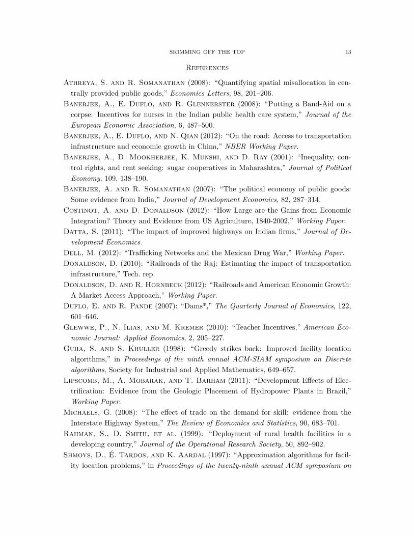
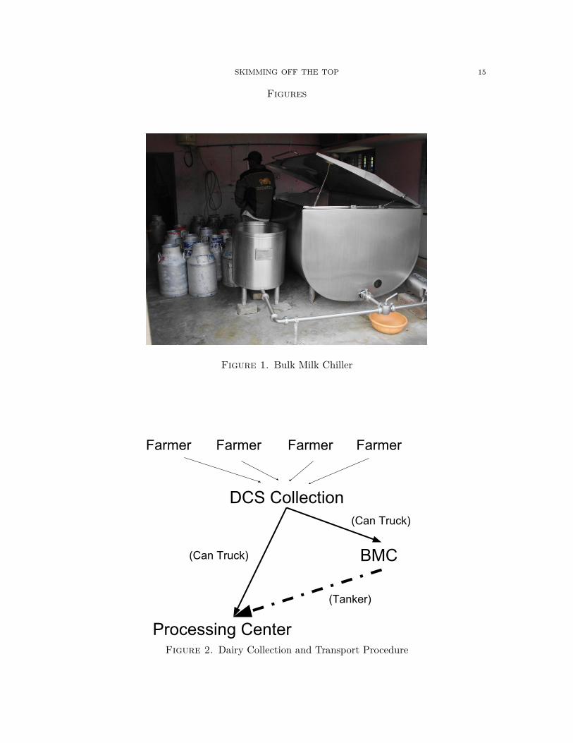
In some villages, the milk cans are loaded onto a truck and delivered directly to one ofthe four district processing plants. There, full-time KMF employees test the milk’s quality,measured by fat and solid non-fat (SNF) levels, and inspect for evidence of dilution oradulteration. In other villages, the milk cans are loaded into trucks and delivered to anearby chilling facility, or bulk milk chiller (BMC). (See Figure 1 for a picture of a BMC.)Milk delivered to BMCs is tested by local DCS officers where the BMC is located. Themilk is then combined with the milk from other villages and chilled. Once per day, arefrigerated tanker truck delivers milk from the chillers to one of the four productionfacilities. The average contents of the refrigerated truck are tested by the full-time KMFemployees, but measurements cannot be traced back to individual villages. Figure 2 detailsthis procurement process in a flow chart.

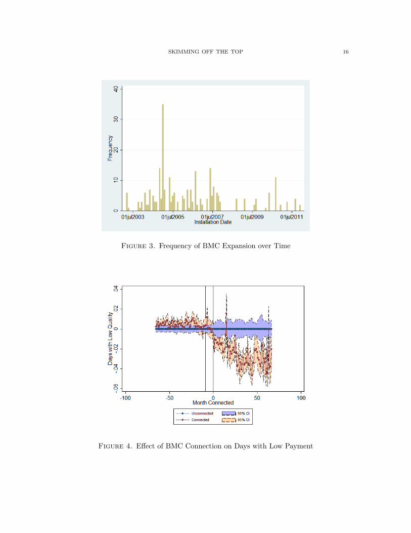
Bulk Milk Chiller (BMC) Expansion. Transportation costs and milk spoilage are signifi-cant barriers to expansion for the KMF. As a result, with the help of the Government ofIndia, the organization has invested heavily in bringing refrigeration technology to remotevillages. Each new BMC constructed produces 5 villages that are connected to refrigeratedtechnology. With the chillers, milk only needs to be collected once daily, further reducingcosts. In the past decade, the KMF has built more than 100 BMCs in the two districtswe study. Figure 3 shows the frequency of new BMCs over time. We seek to estimate thevalue in terms of milk quality and farmer co-investment of a village being connected to aBMC.

It is important to note that the selection criteria for receiving a BMC are not random.Some of the determinants are minimum levels of daily milk procurement, the presenceof other producing villages nearby, ownership of a structure that could accommodate aBMC, proximity to a road where tanker trucks can pass, and reliable power supply. TheKMF banks the biggest gain from installing BMCs farther away from the processing plantswhere sspoilage risk en route to the processor is high.

Incentives for Quality and Milk Pricing. The processing center pays each DCS a prt literrate based on milk quality. The procurement price is increasing in both quality dimensions,fat and SNF. If either the fat or SNF levels fall below some pre-specified threshold, then3The DCS secretary measures the CLR, or corrected lacto-meter reading. This is a temperature-adjusteddensity measure. However, the field test is highly manipulable.


the DCS is punished with a discretely lower payment. Low payment or no payment isalso given if milk is spoiled, though this occurs extremely infrequently in practice. Milkthat is nearly spoiled can only be used for cheap retail products such as highly pasturizedshelf-stable milk packets, and therefore lowers the state organization’s annual profitability.However, individual villages are rarely penalized for such occurrences. Qualitative surveyssuggest that farmers believe spoilage to pose a large threat to their income, perhaps dueto past payment schemes before the availability of high-quality pasturization technology,despite the low prevalence of reported spoilage in the current data.

While village-level milk prices are increasing in quality, two problems limit the powerof these incentives. First, villagers are only paid directly for quantity. They may receiveyear-end bonuses if the average village quality is high, but individual incentives are weak.Furthermore, the power of the quality incentives are quite low in terms of the marginalprice for quality. A 2 standard deviation increase in quality is only accompanied by asmall increase in price, on the order of magnitude of 2%. The incentive is much steeperwhen quality falls below a certain threshold, resulting in a payment decrease of 50 or even100%. Thus, there are hgh returns to producing milk that meets a certain standard, butweak incentives to exceed the standard.

Milk quality and yield are determined by several factors including breed of cow, feedtype, health and vaccination record of the animals, and water availability. Notably, pro-ducers may also choose to dilute their milk to increase their supplied quantity. Becausethinning the milk decreases both fat and SNF, other adulterants may be added with thewater such as milk powder, butter, salt, sugar, urea or even shampoo to avoid detection.Adulterant testing is costly, so only a small subsample of pooled DCS milk is tested, withno payment given for milk found to be adulterated. Anecdotal evidence suggests that milkdilution and adulteration is relatively commonm but rarely punished. External audits sug-gest that in Karnataka, approximately 20% of samples contain adulterants.4 Determiningthe effects of BMC expansion on quality, quantity, and production behavior is a key goalof this paper.

Each DCS’s total earnings comprise the difference between the price received from theKMF and the price paid to the farmer, plus a year-end bonus based on the KMF’s annualprofits. A portion of these earnings go to DCS building maintenance and staff paymentsat the DCS president’s discretion. The remainder are returned to farmers on a per-literbasis, again independent of individual quality.

When a village is connected to a BMC, the monitoring of quality is transferred fromthe processing plant to the village where the BMC is located. Thus, villages connected toa BMC are paid based on measurements taken at the BMC by local officers while villagesthat deliver directly to processing centers are paid based on measurements taken by central

4Times of India, 01/12/2012


staff. This creates additional incentive problems. It is possible that village personnel helptheir own members and the members of contributing DCSs by inflating certain qualityparameters. It is also possible that DCS officials dilute the milk to achieve the highestpossible volume meeting still meeting minimum standard for normal payment. While thebulk milk chiller facilitates market expansion and consolidates transportation costs, it alsodecentralizes the monitoring process.

2.2. Data. We use four main data sources in our analysis.

KMF Administrative Records. The KMF has generously shared administrative recordswith us for the districts of Kolar and Chikballapur. These districts, formerly a singledistrict until 2009, are both managed by the Kolar Milk Union; thus the same policies andprices apply to all villages in the sample. The administrative records detail village-levelquantity and quality for each morning and evening collection from April 1, 2000 to March31, 2011. We restrict analysis to a balanced panel of DCSs that report data in everymonth of the study period, consisting of 842 villages. The reported quality characteristicsinclude fat and SNF as well as the per liter price paid to each DCSs milk on a twice-dailybasis, including penalry payments for low quality or spoilage. The KMF also provided uswith a list of all of the villages with BMCs as of July 2011.

Survey of BMC Villages. Using the list of BMCs provided by the KMF, we surveyed theDCS secretary in each of the 100 villages. From these personnel, we collected the numberof members at the time of the survey, the date of commissioning of the BMC, the date ofinstallation of the BMC, and the names of the other DCSs that contribute milk to theirBMC.

Department of Animal Husbandry Records. To measure the composition of each DCS’sherd of cattle, we obtained livestock census data from the Karnataka Department ofAnimal Husbandry. The organization records detailed information at the village-level ontypes and breeds of cows and buffaloes, along with animal husbandry participation ratesby households in the village. The censuses are collected every 5 years, and we use the2002 and 2007 data in our analysis.

Census of India. Finally, we use data from the 2001 Village Census of India. The keyvariables available from the census are GPS coordinates (used to calculate distances be-tween villages), population, number of scheduled castes and scheduled tribes members,total land area, total cultivated land, and total irrigated land. We are waiting for the2011 village census data to become available so that we can use other variables in ourdiff-in-diff analysis. We supplement the geographical data with GPS coordinates of thefour district milk processing plants read from Google Maps. Census and livesrock censusdata are easily matched using the national census code. These are then matched to the


KMF production data by village name and location. We are able to match 761 out of 842from the KMF records to the census.

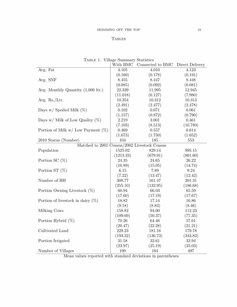
2.3. Descriptive Statistics. Table 1 displays an overview of our final data set. Thefirst column contains means of the pertinent variables for villages that receive a BMCby 2011, the second for villages eventually connected to another village’s BMC, and thethird for never-connected villages. Note that in this sample, 104 villages ever receive aBMC, 185 villages become connected to another village’s BMC, while 553 villages remainunconnected. The average fat levels tend to hover around 4.10 with 8.45 SNF in allcategories of village. The high variance in rate paid stems from rate chart adjustmentsover time (with the average payment increasing from Rs. 10/ltr. to Rs. 18/ltr. over thisperiod) rather than differences between villages. There are substantial differences betweenthe composition of villages which receive a BMC and that of the other two categories. BMCvillages tend to be bigger with smaller scheduled tribes populations. This is not surprisingin light of KMF’s selection criteria.

3. Empirical Strategy: Differences-in-Differences

We first evaluate the village-level production response to chilling centers using regressionanalysis. All regressions are run on a balanced panel of village-month observations rangingfrom April, 2000, to March, 2011, with errors clustered at the village level. In all of ourreduced-form analysis, we employ a differences-in-differences approach. Our key regressionof interest is

yv,t = αv + αt + βconnectedv,t−9 + δconnectedv,t+9 + εv,t

v indexes the village or DCS and t indexes the month. connectedv,t is an indicator forwhether village v in month t is connected to a BMC (either has a BMC in the village ordelivers to a nearby village with one). We also include an extra term, βconnectedv,t+9

to capture anticipatory effects, as each BMC is commissioned approximately 9 monthsbefore the actual equipment is installed. At this stage, village officials may yet be worriedthat the BMC placement decision may be altered based on village performance. However,there is not yet any difference in the technology available.

The coefficient δis the effect of having a BMC on a given outcome, yv,t, relative to thecommissioning period. The full effect of receiving a BMC compared to the period beforecommissioning is captured by the sum of coefficients, β+ δ. Time fixed effects, αt, partialout any time-generated variation, including overall trends and seasonal variation. Villagefixed effects, αt, partial out level differences between villages. The remaining identifyingassumption is that villages that become connected to a BMC would have followed thesame production trend as unconnected villages were they not connected to a BMC.


3.1. Framework. Village incentives change after installation in multiple ways. First,BMC installation lowers the travel time between production and chilling, which signif-icantly shortens the period in which milk may spoil. In practice, reported spoilage isextremely low, accounting for less than 0.04% of milk, and does not significantly changeafter the installation of a BMC. However, anecdotal evidence suggests there is a verypervasive belief that transportation time is strongly linked to dairy payments.5

BMC installation also incurs a large fixed cost, making it very unlikely that a BMC issubsequently removed or replaced. In addition, milk delivered to a BMC is tested by localvillage officers rather than central staff at a processing center. As a result, DCS officialsmay have more scope to manipulate the readings to avoid low payment outcomes.

3.2. Milk Production Outcomes. We are primarily interested in the effect of the com-missioning and the installation of a BMC on milk production and the subsequent in-vestment response of producers. Village-level outcomes include average milk fat, SNFs,monthly volume produced, days in which some milk is flagged as low quality, and totalportion of milk for which villages receive low payment. The first two outcomes representvillage average milk quality, and the third total quantity. The fourth comprises the por-tion of days in which some milk receives low payment, and the fifth the total portion ofmilk for which low payment is received. It is never the case that a village receives lowpayment for its entire milk production in a day. Low payment is only meted to those cansfrom which low measurements are taken; the remaining cans receive full payment. Lowpayment very rarely stems from spoilage; the vast majority of low payment instances arecaused by low quality, as measured by fat and SNF content.

In a story of virtuous BMC effects, we might expect quality (both fat and SNF) toincrease due to less uncertainty about spoilage or rejection ;eading to an increase in effortand decrease in adulteration. Quantity may increase due to more investment, but iffarmers adulterate less following BMC expansion, then quantity may decrease. Similarly,low payments should decrease with the increase in quality.

Alternatively, if the monitoring effects dominate, then we should expect higher paymentsand higher quantities, with no observable increase in the fat or SNF levels, and potentiallyan overall decline in average quality. These outcomes would correspond to a situation inwhich villagers expend minimal effort and dilute milk down to the minimum threshold, andthen monitors bump up any low readings that fall below the regular payment threshold.

3.3. Livestock Outcomes. We supplement our analysis of village-level outcomes usingvillage livestock censuses. In our period of study, censuses were conducted in 2002 and2007. Using these, we implement a simple difference-in-difference taking villages thathad a BMC installed in the interim period as the treatment group and those that were

5It also might be the case that changes in producer incentives offset the virtuous effect on spoilage.


unconnected to a BMC in 2007 as control. If villages respond to chilling facilities byimproving production, we would expect to see a shift in herd composition from indigenouscow varieties to crossbreeds, which require greater investment in feed and care but alsoprovide higher quality milk. Inversely, if BMCs degrade the ability for the KMF to monitorquality, we would expect a decline in livestock investment.

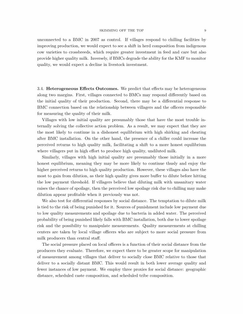
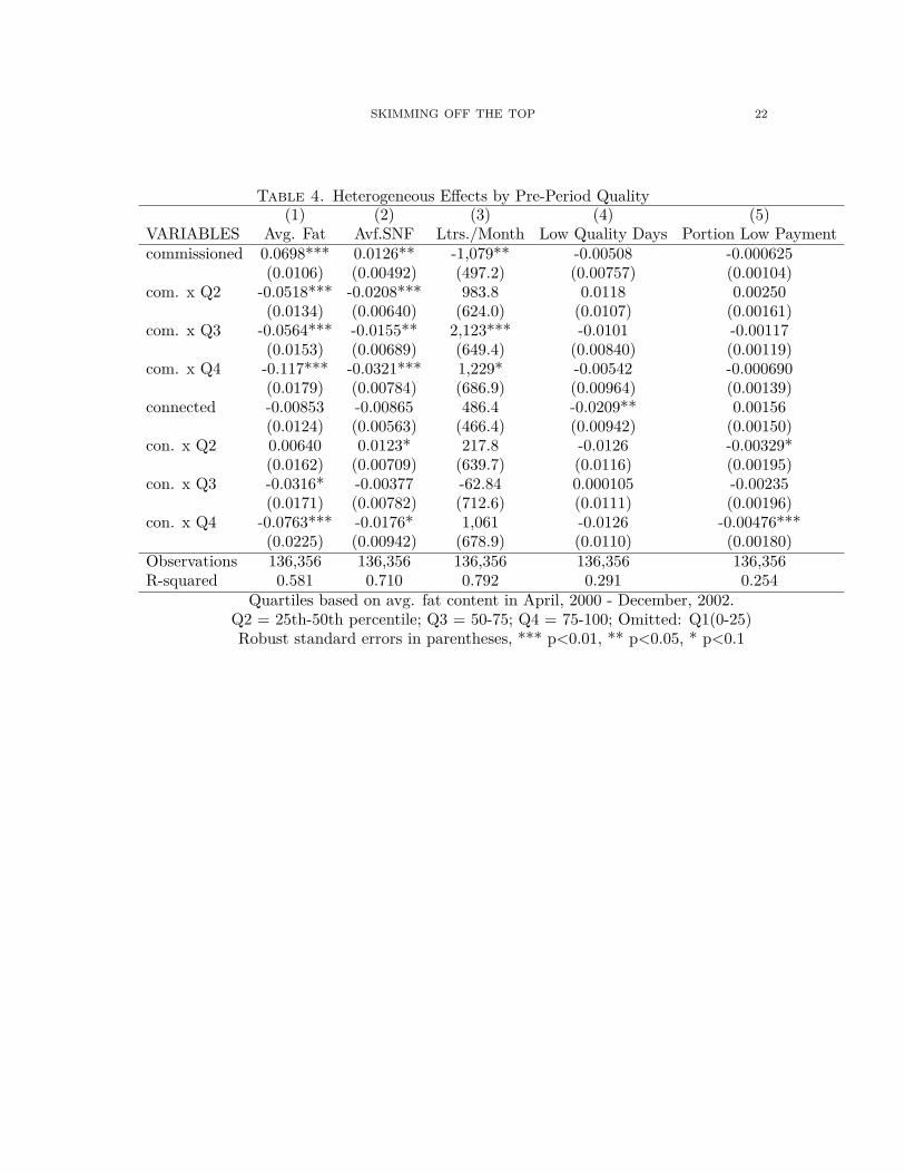
3.4. Heterogeneous Effects Outcomes. We predict that effects may be heterogeneousalong two margins. First, villages connected to BMCs may respond differently based onthe initial quality of their production. Second, there may be a differential response toBMC connection based on the relationship between villagers and the officers responsiblefor measuring the quality of their milk.

Villages with low initial quality are presumably those that have the most trouble in-ternally solving the collective action problem. As a result, we may expect that they arethe most likely to continue in a dishonest equilibrium with high shirking and cheatingafter BMC installation. On the other hand, the presence of a chiller could increase theperceived returns to high quality milk, facilitating a shift to a more honest equilibriumwhere villagers put in high effort to produce high quality, undiluted milk.

Similarly, villages with high initial quality are presumably those initially in a morehonest equilibrium, meaning they may be more likely to continue thusly and enjoy thehigher perceived returns to high quality production. However, these villages also have themost to gain from dilution, as their high quality gives more buffer to dilute before hittingthe low payment threshold. If villagers believe that diluting milk with unsanitary waterraises the chance of spoilage, then the perceived low spoilage risk due to chilling may makedilution appear profitable when it previously was not.

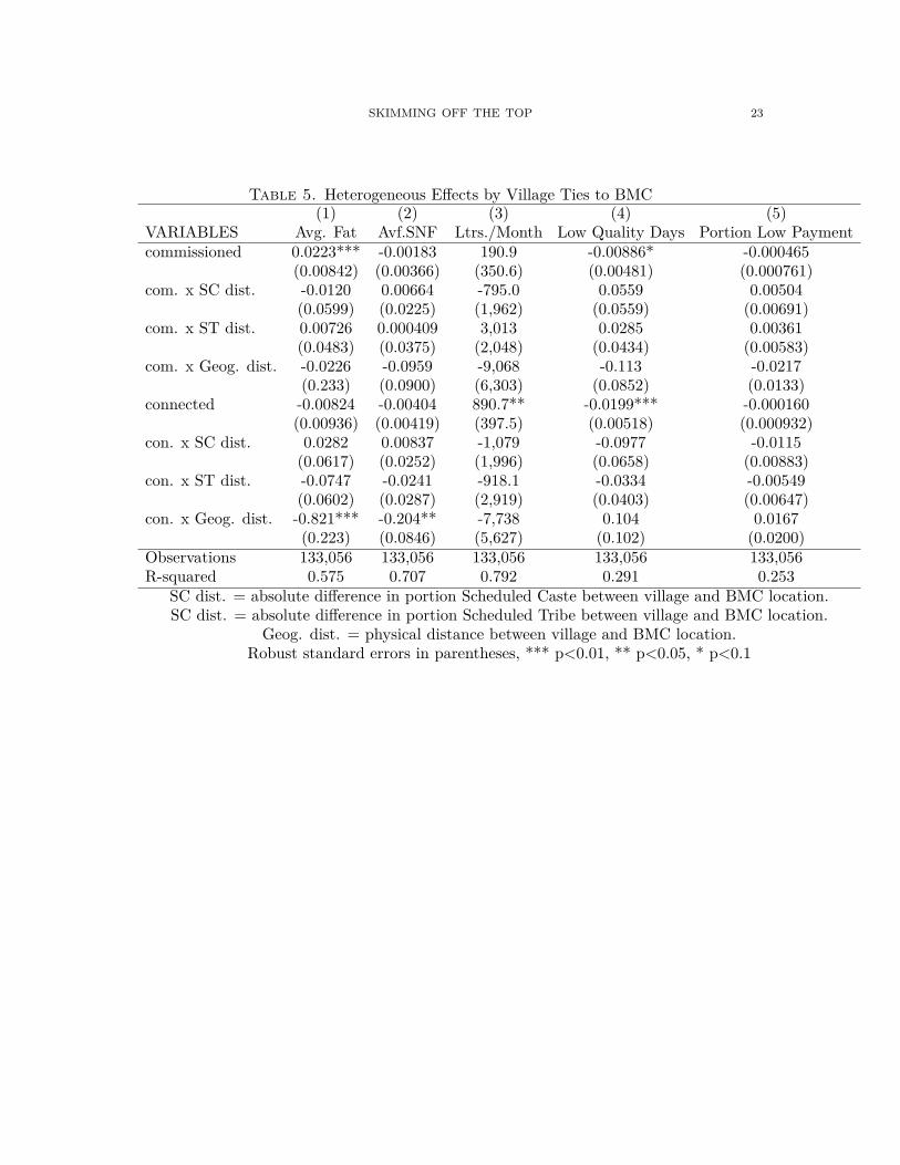
We also test for differential responses by social distance. The temptation to dilute milkis tied to the risk of being punished for it. Sources of punishment include low payment dueto low quality measurements and spoilage due to bacteria in added water. The perceivedprobability of being punished likely falls with BMC installation, both due to lower spoilagerisk and the possibility to manipulate measurements. Quality measurements at chillingcenters are taken by local village officers who are subject to more social pressure frommilk producers than central staff.

The social pressure placed on local officers is a function of their social distance from theproducers they evaluate. Therefore, we expect there to be greater scope for manipulationof measurement among villages that deliver to socially close BMC relative to those thatdeliver to a socially distant BMC. This would result in both lower average quality andfewer instances of low payment. We employ three proxies for social distance: geographicdistance, scheduled caste composition, and scheduled tribe composition.


4. Results: Differences-in-Differences

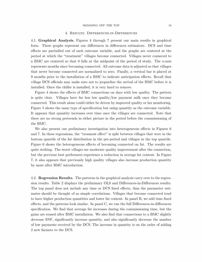
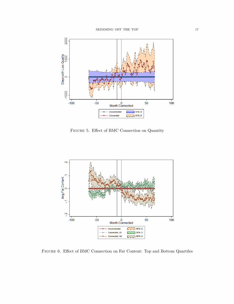
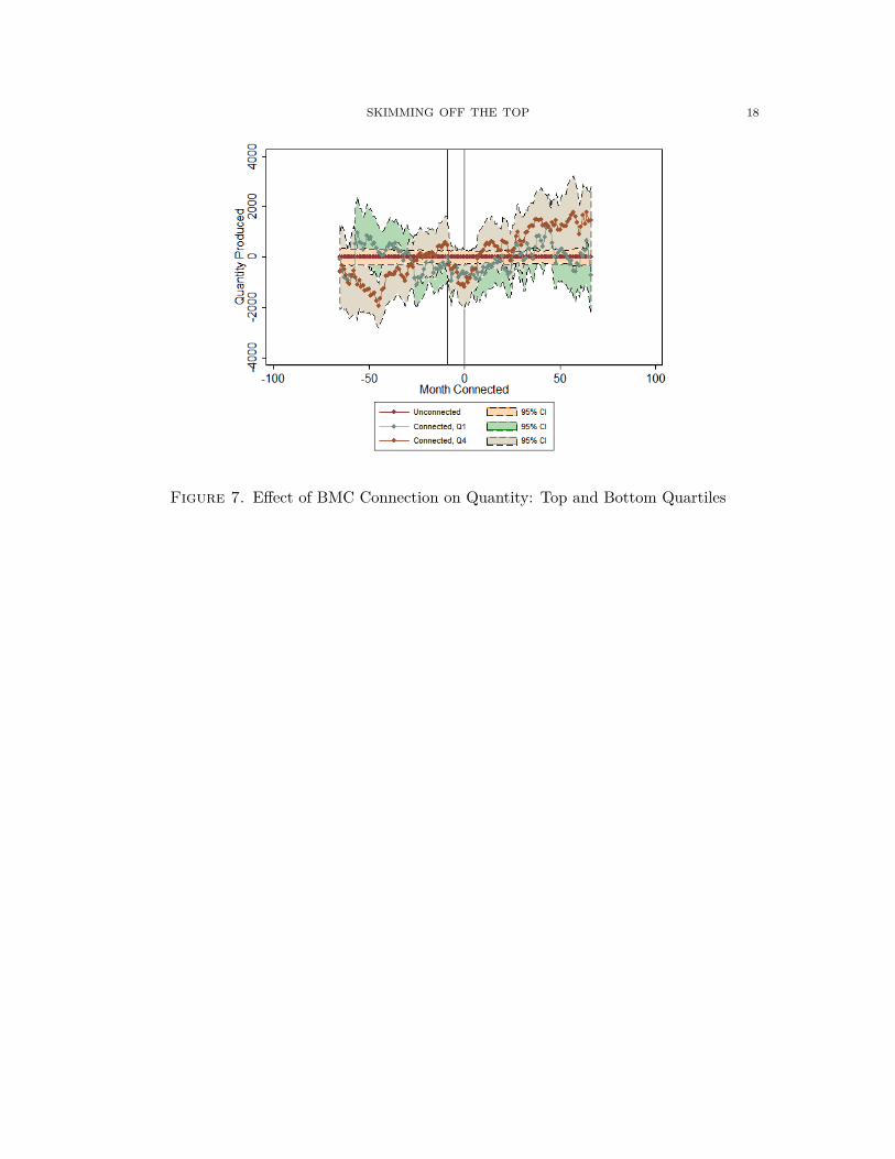
4.1. Graphical Analysis. Figures 4 through 7 present our main results in graphicalform. These graphs represent our differences in differences estimators. DCS and timeeffects are partialled out of each outcome variable, and the graphs are centered at theperiod at which the “treatment” villages become connected. Villages never conneced toa BMC are centered so that 0 falls at the midpoint of the period of study. The x-axisrepresents months since becoming connected. All outcome data is adjusted so that villagesthat never become connected are normalized to zero. Finally, a vertical bar is placed at9 months prior to the installation of a BMC to indicate anticipation effects. Recall thatvillage DCS officials may make sure not to jeopardize the arrival of the BMC before it isinstalled. Once the chiller is installed, it is very hard to remove.

Figure 4 shows the effects of BMC connections on days with low quality. The patternis quite clear. Villages have far less low quality/low payment milk once they becomeconnected. This result alone could either be driven by improved quality or lax monitoring.Figure 5 shows the same type of specification but using quantity as the outcome variable.It appears that quantity increases over time once the villages are connected. Note thatthere are no strong pretrends in either picture in the period before the commissioning ofthe BMC.

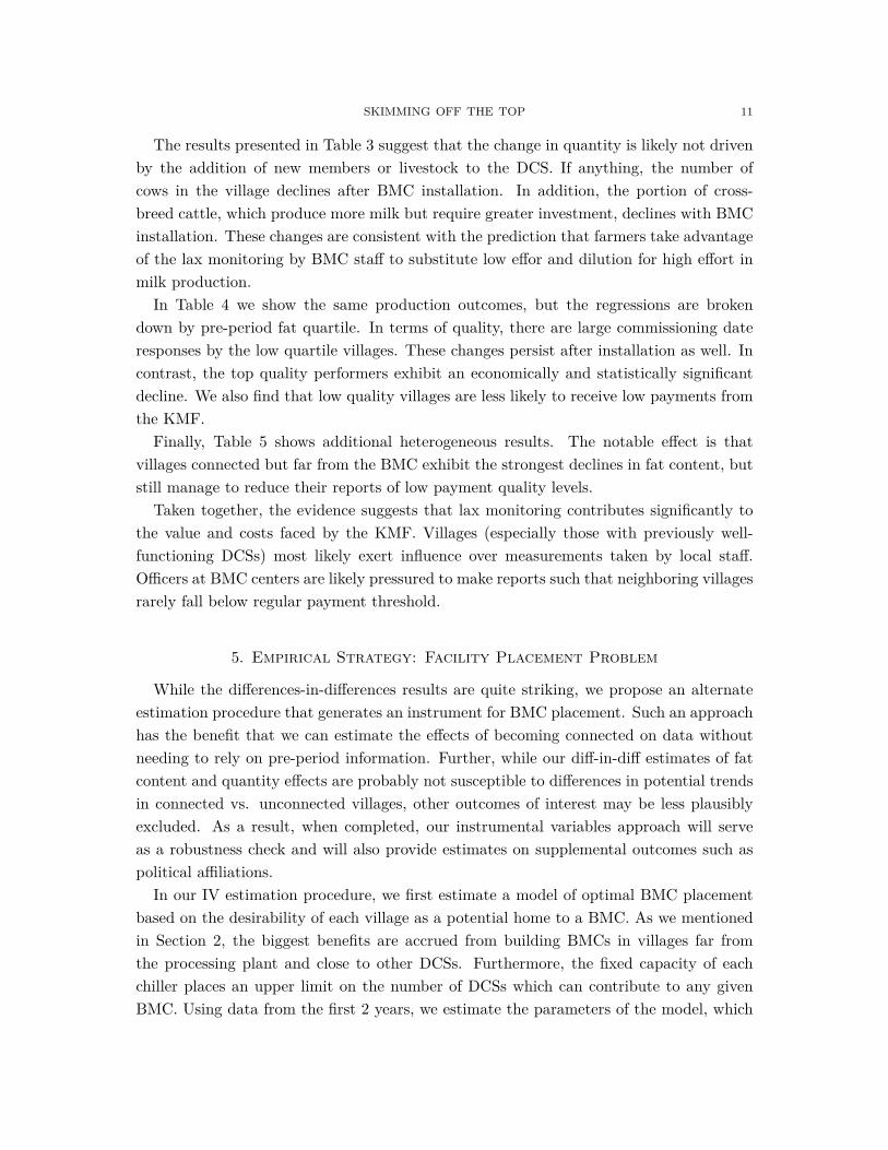
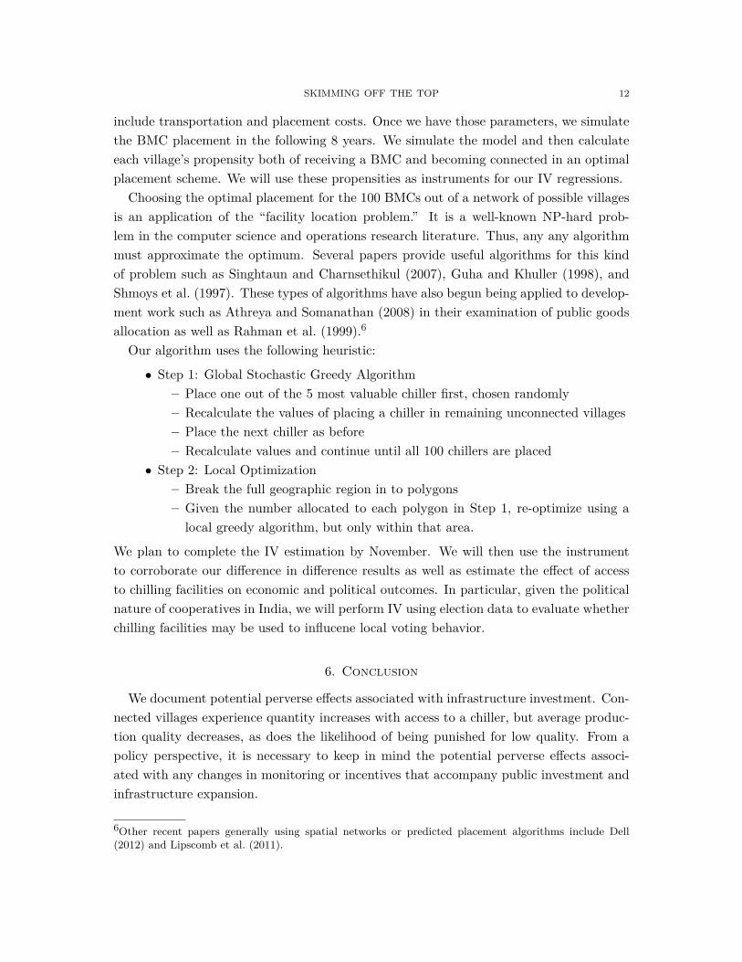
We also present our preliminary investigation into heterogeneous effects in Figures 6and 7. In these regressions, the “treament effect” is split between villages that were in thebottom quartile of the fat distribution in the pre-period and villages in the top quartile.Figure 6 shows the heterogeneous effects of becoming connected on fat. The results arequite striking. The worst villages see moderate quality improvement after the connection,but the previous best performers experience a reduction in average fat content. In Figure7, it also appears that previously high quality villages also increase production quantityby more after BMC introduction.

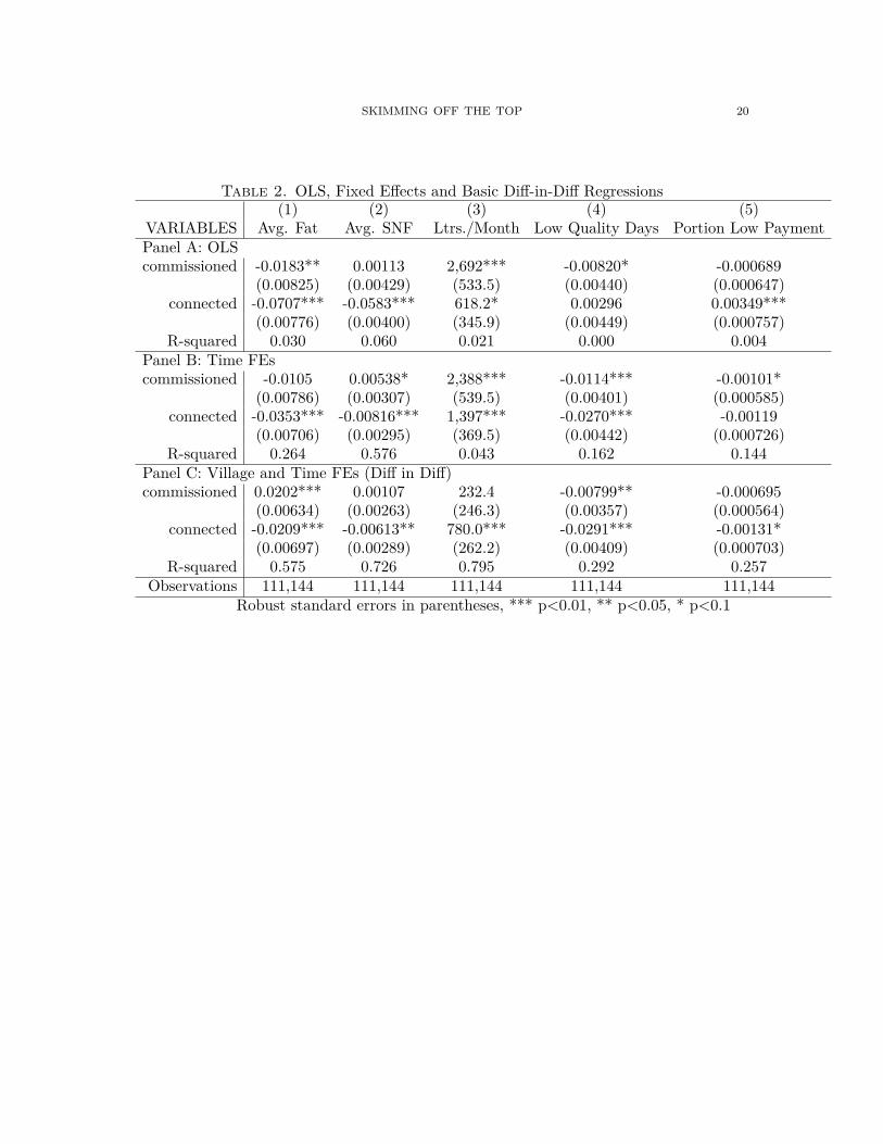
4.2. Regression Results. The patterns in the graphical analysis carry over to the regres-sion results. Table 2 displays the preliminary OLS and Differences-in-Differences results.The top panel does not include any time or DCS fixed effects, thus the parameter esti-mates should be thought of as simple correlations. Villages that become connected tendto have higher production quantities and lower fat content. In panel B, we add time fixedeffects, and the patterns look similar. In panel C, we run the full Differences-in-differencesspecification. We find that average fat increases during the commissioning time, but thegains are erased after BMC installation. We also find that connections to a BMC slightlydecrease SNF, significantly increase quantity, and also significantly decrease the numberof low payments received by the DCS. The increase in quantity is on the order of adding2 new farmers to the DCS.


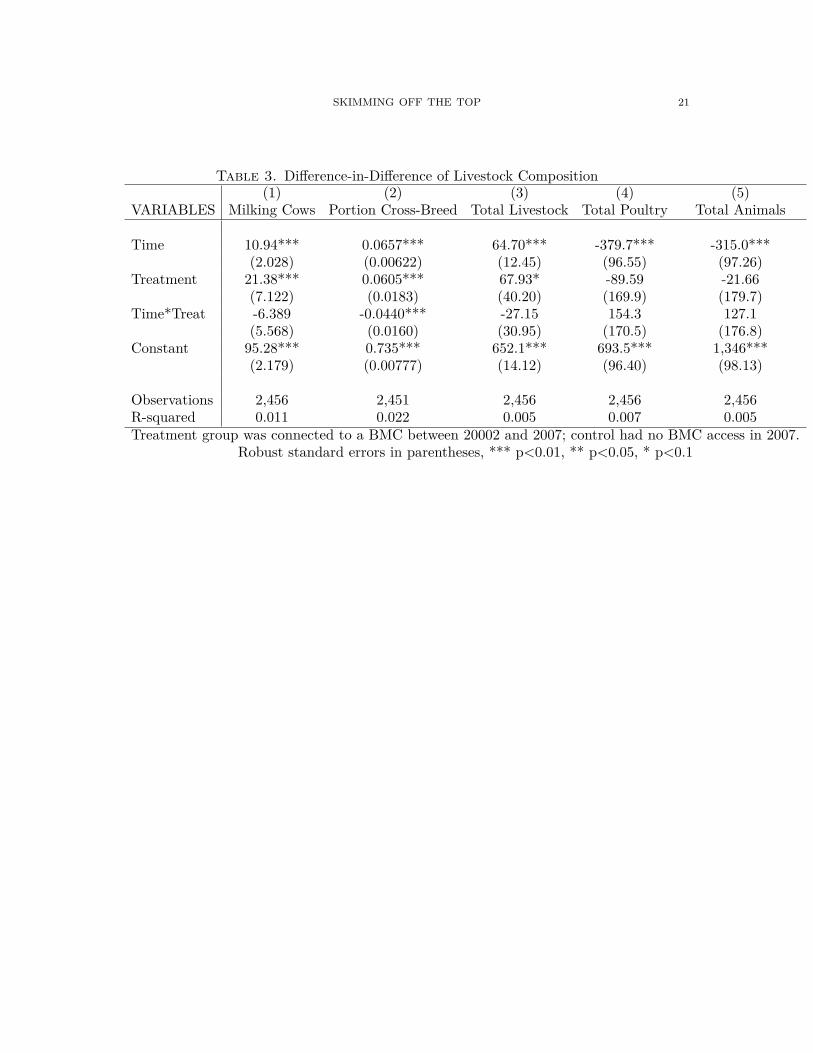
The results presented in Table 3 suggest that the change in quantity is likely not drivenby the addition of new members or livestock to the DCS. If anything, the number ofcows in the village declines after BMC installation. In addition, the portion of cross-breed cattle, which produce more milk but require greater investment, declines with BMCinstallation. These changes are consistent with the prediction that farmers take advantageof the lax monitoring by BMC staff to substitute low effor and dilution for high effort inmilk production.

In Table 4 we show the same production outcomes, but the regressions are brokendown by pre-period fat quartile. In terms of quality, there are large commissioning dateresponses by the low quartile villages. These changes persist after installation as well. Incontrast, the top quality performers exhibit an economically and statistically significantdecline. We also find that low quality villages are less likely to receive low payments fromthe KMF.

Finally, Table 5 shows additional heterogeneous results. The notable effect is thatvillages connected but far from the BMC exhibit the strongest declines in fat content, butstill manage to reduce their reports of low payment quality levels.

Taken together, the evidence suggests that lax monitoring contributes significantly tothe value and costs faced by the KMF. Villages (especially those with previously well-functioning DCSs) most likely exert influence over measurements taken by local staff.Officers at BMC centers are likely pressured to make reports such that neighboring villagesrarely fall below regular payment threshold.

5. Empirical Strategy: Facility Placement Problem

While the differences-in-differences results are quite striking, we propose an alternateestimation procedure that generates an instrument for BMC placement. Such an approachhas the benefit that we can estimate the effects of becoming connected on data withoutneeding to rely on pre-period information. Further, while our diff-in-diff estimates of fatcontent and quantity effects are probably not susceptible to differences in potential trendsin connected vs. unconnected villages, other outcomes of interest may be less plausiblyexcluded. As a result, when completed, our instrumental variables approach will serveas a robustness check and will also provide estimates on supplemental outcomes such aspolitical affiliations.

In our IV estimation procedure, we first estimate a model of optimal BMC placementbased on the desirability of each village as a potential home to a BMC. As we mentionedin Section 2, the biggest benefits are accrued from building BMCs in villages far fromthe processing plant and close to other DCSs. Furthermore, the fixed capacity of eachchiller places an upper limit on the number of DCSs which can contribute to any givenBMC. Using data from the first 2 years, we estimate the parameters of the model, which


include transportation and placement costs. Once we have those parameters, we simulatethe BMC placement in the following 8 years. We simulate the model and then calculateeach village’s propensity both of receiving a BMC and becoming connected in an optimalplacement scheme. We will use these propensities as instruments for our IV regressions.

Choosing the optimal placement for the 100 BMCs out of a network of possible villagesis an application of the “facility location problem.” It is a well-known NP-hard prob-lem in the computer science and operations research literature. Thus, any any algorithmmust approximate the optimum. Several papers provide useful algorithms for this kindof problem such as Singhtaun and Charnsethikul (2007), Guha and Khuller (1998), andShmoys et al. (1997). These types of algorithms have also begun being applied to develop-ment work such as Athreya and Somanathan (2008) in their examination of public goodsallocation as well as Rahman et al. (1999).6

Our algorithm uses the following heuristic:

• Step 1: Global Stochastic Greedy Algorithm– Place one out of the 5 most valuable chiller first, chosen randomly– Recalculate the values of placing a chiller in remaining unconnected villages– Place the next chiller as before– Recalculate values and continue until all 100 chillers are placed

• Step 2: Local Optimization– Break the full geographic region in to polygons– Given the number allocated to each polygon in Step 1, re-optimize using a

local greedy algorithm, but only within that area.

We plan to complete the IV estimation by November. We will then use the instrumentto corroborate our difference in difference results as well as estimate the effect of accessto chilling facilities on economic and political outcomes. In particular, given the politicalnature of cooperatives in India, we will perform IV using election data to evaluate whetherchilling facilities may be used to influcene local voting behavior.

6. Conclusion

We document potential perverse effects associated with infrastructure investment. Con-nected villages experience quantity increases with access to a chiller, but average produc-tion quality decreases, as does the likelihood of being punished for low quality. From apolicy perspective, it is necessary to keep in mind the potential perverse effects associ-ated with any changes in monitoring or incentives that accompany public investment andinfrastructure expansion.

6Other recent papers generally using spatial networks or predicted placement algorithms include Dell(2012) and Lipscomb et al. (2011).


References

Athreya, S. and R. Somanathan (2008): “Quantifying spatial misallocation in cen-trally provided public goods,” Economics Letters, 98, 201–206.

Banerjee, A., E. Duflo, and R. Glennerster (2008): “Putting a Band-Aid on acorpse: Incentives for nurses in the Indian public health care system,” Journal of theEuropean Economic Association, 6, 487–500.

Banerjee, A., E. Duflo, and N. Qian (2012): “On the road: Access to transportationinfrastructure and economic growth in China,” NBER Working Paper.

Banerjee, A., D. Mookherjee, K. Munshi, and D. Ray (2001): “Inequality, con-trol rights, and rent seeking: sugar cooperatives in Maharashtra,” Journal of PoliticalEconomy, 109, 138–190.

Banerjee, A. and R. Somanathan (2007): “The political economy of public goods:Some evidence from India,” Journal of Development Economics, 82, 287–314.

Costinot, A. and D. Donaldson (2012): “How Large are the Gains from EconomicIntegration? Theory and Evidence from US Agriculture, 1840-2002,” Working Paper.

Datta, S. (2011): “The impact of improved highways on Indian firms,” Journal of De-velopment Economics.

Dell, M. (2012): “Trafficking Networks and the Mexican Drug War,” Working Paper.Donaldson, D. (2010): “Railroads of the Raj: Estimating the impact of transportationinfrastructure,” Tech. rep.

Donaldson, D. and R. Hornbeck (2012): “Railroads and American Economic Growth:A Market Access Approach,” Working Paper.

Duflo, E. and R. Pande (2007): “Dams*,” The Quarterly Journal of Economics, 122,601–646.

Glewwe, P., N. Ilias, and M. Kremer (2010): “Teacher Incentives,” American Eco-nomic Journal: Applied Economics, 2, 205–227.

Guha, S. and S. Khuller (1998): “Greedy strikes back: Improved facility locationalgorithms,” in Proceedings of the ninth annual ACM-SIAM symposium on Discretealgorithms, Society for Industrial and Applied Mathematics, 649–657.

Lipscomb, M., A. Mobarak, and T. Barham (2011): “Development Effects of Elec-trification: Evidence from the Geologic Placement of Hydropower Plants in Brazil,”Working Paper.

Michaels, G. (2008): “The effect of trade on the demand for skill: evidence from theInterstate Highway System,” The Review of Economics and Statistics, 90, 683–701.

Rahman, S., D. Smith, et al. (1999): “Deployment of rural health facilities in adeveloping country,” Journal of the Operational Research Society, 50, 892–902.

Shmoys, D., É. Tardos, and K. Aardal (1997): “Approximation algorithms for facil-ity location problems,” in Proceedings of the twenty-ninth annual ACM symposium on


Theory of computing, ACM, 265–274.Singhtaun, C. and P. Charnsethikul (2007): “An efficient algorithm for capacitatedmultifacility location problems,” Journal of Computer Science, 3, 583–591.


Figures

Figure 1. Bulk Milk Chiller

Farmer

DCS Collection

FarmerFarmerFarmer

Processing Center

BMC

(Can Truck)

(Can Truck)

(Tanker)

Figure 2. Dairy Collection and Transport Procedure


Figure 3. Frequency of BMC Expansion over Time

Figure 4. Effect of BMC Connection on Days with Low Payment


Figure 5. Effect of BMC Connection on Quantity

Figure 6. Effect of BMC Connection on Fat Content: Top and Bottom Quartiles


Figure 7. Effect of BMC Connection on Quantity: Top and Bottom Quartiles


Tables

Table 1. Village Summary StatisticsWith BMC Connected to BMC Direct Delivery

Avg. Fat 4.105 4.010 4.123(0.160) (0.178) (0.191)

Avg. SNF 8.455 8.447 8.448(0.085) (0.092) (0.081)

Avg. Monthly Quantity (1,000 ltr.) 22.339 11.995 12.945(11.018) (6.127) (7.980)

Avg. Rs./Ltr. 10.354 10.312 10.313(2.491) (2.477) (2.478)

Days w/ Spoiled Milk (%) 0.102 0.071 0.061(1.157) (0.872) (0.790)

Days w/ Milk of Low Quality (%) 2.219 3.001 0.461(7.103) (8.513) (10.780)

Portion of Milk w/ Low Payment (%) 0.469 0.557 0.614(1.673) (1.750) (1.652)

2010 Status (Number) 104 185 553Matched to 2001 Census/2002 Livestock Census

Population 1525.02 829.14 995.15(1213.33) (679.91) (861.60)

Portion SC (%) 24.35 24.65 26.22(10.89) (15.05) (14.74)

Portion ST (%) 6.15 7.89 9.24(7.22) (13.47) (12.42)

Number of HH 308.77 161.47 201.31(255.10) (132.95) (186.68)

Portion Owning Livestock (%) 60.94 66.03 65.59(17.60) (17.19) (17.67)

Portion of livestock in dairy (%) 18.82 17.14 16.86(9.18) (8.83) (8.46)

Milking Cows 158.82 94.00 112.23(109.69) (50.37) (77.35)

Portion Hybrid (%) 70.26 64.46 57.01(20.47) (22.28) (21.21)

Cultivated Land 229.23 181.16 179.78(193.32) (136.73) (343.83)

Portion Irrigated 31.58 32.61 32.94(23.97) (25.19) (25.03)

Number of Villages 100 164 497Mean values reported with standard deviations in parentheses.


Table 2. OLS, Fixed Effects and Basic Diff-in-Diff Regressions(1) (2) (3) (4) (5)

VARIABLES Avg. Fat Avg. SNF Ltrs./Month Low Quality Days Portion Low PaymentPanel A: OLScommissioned -0.0183** 0.00113 2,692*** -0.00820* -0.000689

(0.00825) (0.00429) (533.5) (0.00440) (0.000647)connected -0.0707*** -0.0583*** 618.2* 0.00296 0.00349***

(0.00776) (0.00400) (345.9) (0.00449) (0.000757)R-squared 0.030 0.060 0.021 0.000 0.004

Panel B: Time FEscommissioned -0.0105 0.00538* 2,388*** -0.0114*** -0.00101*

(0.00786) (0.00307) (539.5) (0.00401) (0.000585)connected -0.0353*** -0.00816*** 1,397*** -0.0270*** -0.00119

(0.00706) (0.00295) (369.5) (0.00442) (0.000726)R-squared 0.264 0.576 0.043 0.162 0.144

Panel C: Village and Time FEs (Diff in Diff)commissioned 0.0202*** 0.00107 232.4 -0.00799** -0.000695

(0.00634) (0.00263) (246.3) (0.00357) (0.000564)connected -0.0209*** -0.00613** 780.0*** -0.0291*** -0.00131*

(0.00697) (0.00289) (262.2) (0.00409) (0.000703)R-squared 0.575 0.726 0.795 0.292 0.257

Observations 111,144 111,144 111,144 111,144 111,144Robust standard errors in parentheses, *** p<0.01, ** p<0.05, * p<0.1


Table 3. Difference-in-Difference of Livestock Composition(1) (2) (3) (4) (5)

VARIABLES Milking Cows Portion Cross-Breed Total Livestock Total Poultry Total Animals

Time 10.94*** 0.0657*** 64.70*** -379.7*** -315.0***(2.028) (0.00622) (12.45) (96.55) (97.26)

Treatment 21.38*** 0.0605*** 67.93* -89.59 -21.66(7.122) (0.0183) (40.20) (169.9) (179.7)

Time*Treat -6.389 -0.0440*** -27.15 154.3 127.1(5.568) (0.0160) (30.95) (170.5) (176.8)

Constant 95.28*** 0.735*** 652.1*** 693.5*** 1,346***(2.179) (0.00777) (14.12) (96.40) (98.13)

Observations 2,456 2,451 2,456 2,456 2,456R-squared 0.011 0.022 0.005 0.007 0.005Treatment group was connected to a BMC between 20002 and 2007; control had no BMC access in 2007.

Robust standard errors in parentheses, *** p<0.01, ** p<0.05, * p<0.1


Table 4. Heterogeneous Effects by Pre-Period Quality(1) (2) (3) (4) (5)

VARIABLES Avg. Fat Avf.SNF Ltrs./Month Low Quality Days Portion Low Paymentcommissioned 0.0698*** 0.0126** -1,079** -0.00508 -0.000625

(0.0106) (0.00492) (497.2) (0.00757) (0.00104)com. x Q2 -0.0518*** -0.0208*** 983.8 0.0118 0.00250

(0.0134) (0.00640) (624.0) (0.0107) (0.00161)com. x Q3 -0.0564*** -0.0155** 2,123*** -0.0101 -0.00117

(0.0153) (0.00689) (649.4) (0.00840) (0.00119)com. x Q4 -0.117*** -0.0321*** 1,229* -0.00542 -0.000690

(0.0179) (0.00784) (686.9) (0.00964) (0.00139)connected -0.00853 -0.00865 486.4 -0.0209** 0.00156

(0.0124) (0.00563) (466.4) (0.00942) (0.00150)con. x Q2 0.00640 0.0123* 217.8 -0.0126 -0.00329*

(0.0162) (0.00709) (639.7) (0.0116) (0.00195)con. x Q3 -0.0316* -0.00377 -62.84 0.000105 -0.00235

(0.0171) (0.00782) (712.6) (0.0111) (0.00196)con. x Q4 -0.0763*** -0.0176* 1,061 -0.0126 -0.00476***

(0.0225) (0.00942) (678.9) (0.0110) (0.00180)Observations 136,356 136,356 136,356 136,356 136,356R-squared 0.581 0.710 0.792 0.291 0.254

Quartiles based on avg. fat content in April, 2000 - December, 2002.Q2 = 25th-50th percentile; Q3 = 50-75; Q4 = 75-100; Omitted: Q1(0-25)Robust standard errors in parentheses, *** p<0.01, ** p<0.05, * p<0.1


Table 5. Heterogeneous Effects by Village Ties to BMC(1) (2) (3) (4) (5)

VARIABLES Avg. Fat Avf.SNF Ltrs./Month Low Quality Days Portion Low Paymentcommissioned 0.0223*** -0.00183 190.9 -0.00886* -0.000465

(0.00842) (0.00366) (350.6) (0.00481) (0.000761)com. x SC dist. -0.0120 0.00664 -795.0 0.0559 0.00504

(0.0599) (0.0225) (1,962) (0.0559) (0.00691)com. x ST dist. 0.00726 0.000409 3,013 0.0285 0.00361

(0.0483) (0.0375) (2,048) (0.0434) (0.00583)com. x Geog. dist. -0.0226 -0.0959 -9,068 -0.113 -0.0217

(0.233) (0.0900) (6,303) (0.0852) (0.0133)connected -0.00824 -0.00404 890.7** -0.0199*** -0.000160

(0.00936) (0.00419) (397.5) (0.00518) (0.000932)con. x SC dist. 0.0282 0.00837 -1,079 -0.0977 -0.0115

(0.0617) (0.0252) (1,996) (0.0658) (0.00883)con. x ST dist. -0.0747 -0.0241 -918.1 -0.0334 -0.00549

(0.0602) (0.0287) (2,919) (0.0403) (0.00647)con. x Geog. dist. -0.821*** -0.204** -7,738 0.104 0.0167

(0.223) (0.0846) (5,627) (0.102) (0.0200)Observations 133,056 133,056 133,056 133,056 133,056R-squared 0.575 0.707 0.792 0.291 0.253

SC dist. = absolute difference in portion Scheduled Caste between village and BMC location.SC dist. = absolute difference in portion Scheduled Tribe between village and BMC location.

Geog. dist. = physical distance between village and BMC location.Robust standard errors in parentheses, *** p<0.01, ** p<0.05, * p<0.1

skimming off the topneudc2012/docs/paper_275.pdf · skimming off the top: ... the data span a rapid...

Documents