size of giant component in random geometric graphs -g. ganesan indian statistical institute, delhi
TRANSCRIPT

Size of giant component in Random Geometric Graphs
-G. GanesanIndian Statistical Institute, Delhi.

Random Geometric Graph
• n nodes uniformly distributed in S = [-½, ½]2
• Two nodes u and v connected by an edge if d(u, v) < rn
• Resulting graph random geometric graph (RGG)

Figure 1: Random Geometric Graph

Radius of Connectivity

Giant Component Regime
rn
Dense, fully connected
Sparse, noGiant Comp.
2nnr
2
2 log
n
n
nr
nAnrnAnrn log2
Intermediate,Has giant component

Intermediate range

Theorem 1 (Ganesan, 2012)

Proof Sketch of Theorem 1• Divide S into small squares {Si}i
each of size
• Choose 4 < ∆ < 5 so that nodes in adjacent squares are joined by an edge.
• Say that Si is occupied if it contains at least one node and vacant otherwise.
nn rr
S

• Also, divide the unit square S into ``horizontal” rect. each of size
where
• Fix the bottom rectangle R
1n
n
rMK
S
R
n
n
rMK
2
log
nn nr
nK

1
n
n
rMK
SSay that a sequence of occupied squares L = (S1,…,St) form a occupied left-right crossing of R if: (i)Si and Si+1 share an edge for each i.(ii)S1 intersects left edge of R. (iii) St intersects right edge of R.
S1
St

1
n
n
rMK

Probability of left-right crossing
• Let LR(R) denote the event that R has an occupied left-right crossing…
• Lemma (Ganesan, 2012): We have that
for some positive constant δ.
MnRLR
11))(Pr(

• Thus we have that
if M is sufficiently large.
10
11)Pr(n
1
n
n
rMK

• What is the advantage of identifying occupied left-right crossings..
• Ans: We get a path of edges from left to right…

n
n
rMK
1

n
n
rMK
1

Thus
10
11)Pr(n

• What is the probability that each rectangle has such a path?
• Ans: 10
.#1
n
rect

Number of rectangles is
• The number of rectangles is less than
since by our choice of rn, we have
c
n
rr nn
55
cnrn 2
)( nO

• Thus…• The event that each rectangle has an occupied
left-right crossing occurs with prob.
• And we then get a network of paths from left to right…
910
11
)(1
nn
nO

n
n
rMK
1

Thus
910
11
)(1)Pr(
nn
nO
10
11)Pr(n

• Perform an analogous procedure vertically…

n
n
rMK
1

Thus
910
11
)(1)Pr(
nn
nO
10
11)Pr(n
9
21)Pr(n

Why is this useful?
• We have obtained a connected “backbone” of paths in G…
• We have essentially “trapped” isolated components of G in boxes of size…
n
nn
n
rMK
rMK 22

Isolated component
n
n
rMK2
n
n
rMK2

• So, we know that if backbone occurs…
then all components not attached to backbone are “boxable” ,i.e.,
can be fitted in a
box…
n
nn
n
rMK
rMK 22

• Let X denote the sum of size of all components of G that are boxable…
for some positive constants
22
)Pr( nn nrnr eneX
,
(1)
9
21)Pr(n
• Recall that backbone occurs with prob..

Thus
Note: Whenever backbone occurs, X denotes total sum of sizes of components not attached to the backbone…
Therefore
22
9
21)Pr( nn nrnr en
neX
22
9
21)
Pr(
nn nrnr en
nodesnenleastatcontains
backbonetoattachedcomponent

• We need to prove the estimate (1) regarding sum of sizes of boxable components…
i.e. to prove that22
)Pr( nn nrnr eneX Recall: X sum of size of all components of G that are boxable
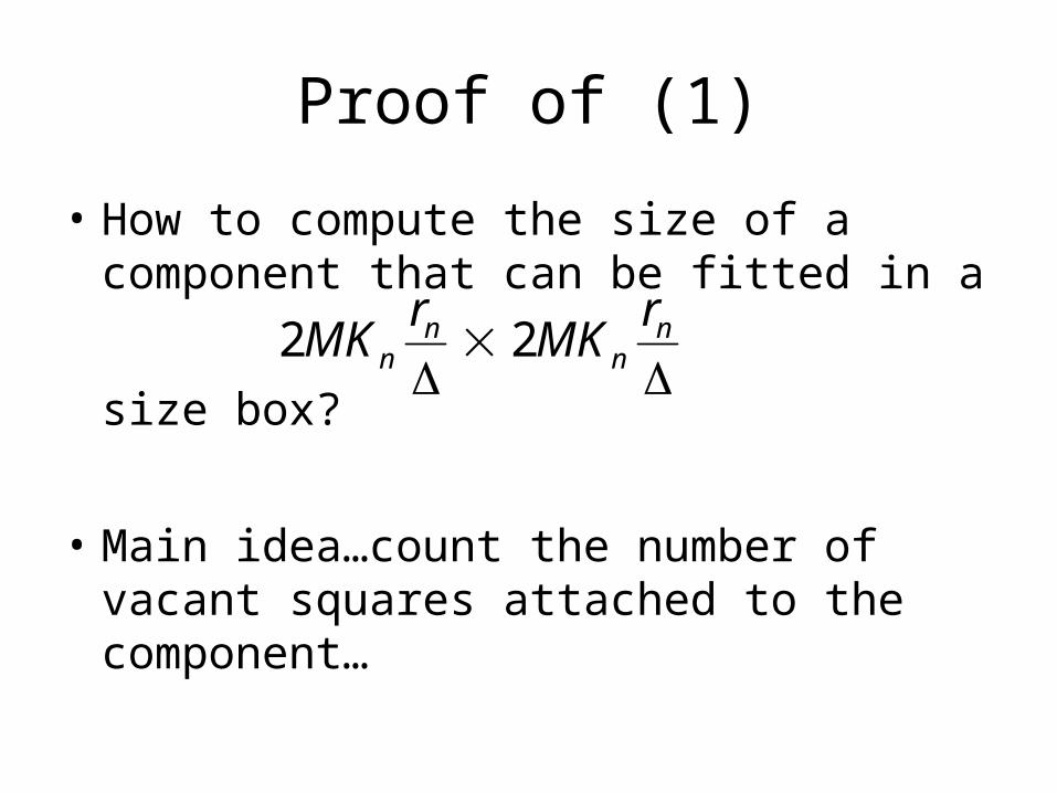
Proof of (1)
• How to compute the size of a component that can be fitted in a
size box?
• Main idea…count the number of vacant squares attached to the component…
n
nn
n
rMK
rMK 22

n
n
rMK2
n
n
rMK2

• Observation from figure…
• “Boxable” components have a circuit of vacant squares attached to them…
• For any square Si
)exp()Pr( 2ni nrvacantS
(proved using standard binomial estimates)

• We therefore cannot have large boxable components…
• Because, such components have a lot of vacant squares ``attached” to them…

More precise computation
• Let S0 be the square containing the origin…
• Define C0 to be the maximal connected set of occupied squares containing S0…
• We say that C0 is the cluster containing S0…

S0C0

S0

• We count the number of vacant squares Vs attached to C0
• Suppose C0 contains k squares
and the outermost boundary ∂C0 of C0 contains
L edges…(thick line in fig.)

The following hold:
• (1) The number of distinct vacant squares attached to ∂C0 is at least Vs > L/8…
• (2) Since ∂C0 contains k squares in its interior, we must have 4
kL

• (3) Also, the ``last edge” of ∂C0 can cut the X axis at at most L distinct points…
• (4) And ∂C0 has a self-avoiding path of L-1 steps.
• (5) The number of choices of ∂C0 is therefore at most L.4L-1

S0Lastedge

• Thus (1)-(5) implies
)exp(
)8/exp(..4)Pr(#
2
4/
210
knr
lnrlkC
n
kln
l

• Thus….
• And if N(C0) denotes the number of nodes is C0, we also have
)exp(# 210 nnrCE
)exp()( 21
20 nn nrnrCEN

• Recall C0 is the occupied cluster containing S0…
• Define Ci for each square Si
• Same conclusion holds…

• Use Markov’s inequality to get…
for θ sufficiently small…
• But is the sum of size of all boxable components…
• And we are done…
22
2
)(Pr nn nrnr
ii AeneCN
i iCN )(

Main summary of steps• (1) We constructed a backbone of paths with high
prob..…
• (2) We deduced that each component not attached to the backbone is “boxable”
• (3) We showed that the sum of sizes of all “boxable” components is less thanwith high prob…
2nnrne

References• M. Franceschetti, O. Dousse, D. N. C. Tse and P. Thiran. (2007). Closing
Gap in the Capacity of Wireless Networks via Percolation Theory. IEEE Trans. Inform. Theory, 53, 1009–1018.
• G. Ganesan. (2012). Size of the giant component in a random geometric graph. Accepted for publ. Ann. Inst. Henri Poincare.
• A. Gopalan, S. Banerjee, A. K. Das and S. Shakottai. (2011). Random Mobility and the Spread of Infection. Proc. IEEE Infocomm, pp. 999–1007.

• P. Gupta and P. R. Kumar. (1998). Critical Power for Asymptotic Connectivity in Wireless Networks. Stoch. Proc. and Appl., 2203–2214.
• M. Penrose. (2003). Random Geometric Graphs. Oxford.