site index in agroforestry systems: age-dependent and age

Site index in agroforestry systems: age-dependentand age-independent dynamic diameter growthmodels for Quercus ilex in Iberian open oakwoodlands

G. Gea-Izquierdo, I. Canellas, and G. Montero

Abstract: Despite Quercus ilex L. being one of the most widespread tree species in the Mediterranean basin, there are nogrowth models in the literature for this species. In this study, we compare age-dependent and age-independent dynamic di-ameter growth models and discuss the concept of dominance in open stands. A posteriori dominance was determined to fitpotential age-dependent growth models and a site index based on diameter growth was defined. Formulations derived frompower decline base models (Korf and Hossfeld) best described diameter growth. The best approach for age-dependentmodels was a polymorphic and with variable asymptotes generalized algebraic difference approach formulation. Residualerrors in trees between 20 and 55 cm ranged from ~7.0% in potential growth models to ~15% in age-independent modelsexpanded by density. Using a unique age-dependent dynamic equation for all trees, regardless of dominance, did not in-crease the error very much. In age-independent models, the inclusion of the defined site index reduced the prediction errorbut requires that the age of trees is estimated to determine the site index. The difficulty of estimating Q. ilex age makesage-independent models very attractive for system modelling. Age-independent models could be useful in other ecosystemswhere age estimation is problematic.

Resume : Bien que Quercus ilex L. soit une des essences les plus repandues dans le bassin mediterraneen, la litteraturen’offre pas de modele de croissance pour cette essence. Dans cette etude, nous comparons les modeles dynamiques decroissance diametrale dependants et independants de l’age et nous discutons du concept de dominance en peuplements ou-verts. Une dominance a posteriori est determinee pour ajuster les modeles de croissance potentielle dependants de l’age.En outre, un indice de qualite de station base sur la croissance diametrale est developpe. Les formulations mathematiquesderivees des equations a puissance decroissante (Korf et Hossfeld) decrivent le mieux la croissance diametrale. La meil-leure approche pour les modeles dependants de l’age est celle de la formulation polymorphique a asymptote variable parla methode de la difference algebrique generalisee. L’erreur residuelle pour les arbres de 20 a 55 cm varie d’environ 7 %pour les modeles de croissance potentielle a environ 15 % pour les modeles independants de l’age avec l’ajout de la den-site. L’emploi d’une equation unique dependante de l’age pour tous les arbres, sans egard a leur dominance, ne fait pasbeaucoup augmenter l’erreur. L’inclusion de l’indice de qualite de station dans les modeles independants de l’age reduitl’erreur de prevision, mais requiert l’estimation de l’age des arbres pour determiner l’indice de qualite de station. La diffi-culte a estimer l’age de Q. ilex rend les modeles independants de l’age tres attrayants pour modeliser sa croissance. Lesmodeles independants de l’age pourraient etre utiles dans d’autres ecosystemes ou l’age est difficile a evaluer.

[Traduit par la Redaction]

Introduction

Agroforestry systems share the presence of a woody com-ponent, commonly trees, and occupy large expanses acrossthe world (Mosquera et al. 2005). Agrosilvopastoral and sil-vopastoral systems are different types of agroforestry sys-tems having in common the presence of grazing animals.Management of these systems differs from that of classicalforestry systems. Usually, timber is not the most importantoutput, which is the reason why tree growth has not been

paid as much attention as in traditional forest systems. Yet,understanding past tree growth is one of the first steps tosustainable management and prediction of future landscaperesponses to different management or climate change sce-narios. Site index models based on the height growth ofdominant trees are the classical way of indirectly estimatingsite quality (mostly a combination of soil fertility and cli-mate) in forestry management (e.g., Carmean 1975; Goelzand Burk 1992; Cieszewski and Bailey 2000). Applying thesite index to modelling the tree component in agroforestrysystems is not always straightforward. Compared with for-ests, agroforestry systems are characterized by low tree den-sities, as other products (e.g., pasture, crops, fruits, cork) areusually of greater economical interest than the timber (Aresand Brauer 2004; Mosquera et al. 2005). Additionally, insome agroforestry systems, trees are pruned (e.g., Balandierand Dupraz 1999) and some of them have originated fromfire or thinned ‘‘natural’’ forests or shrublands. This compli-

Received 5 March 2007. Accepted 23 July 2007. Published onthe NRC Research Press Web site at cjfr.nrc.ca on 25 January2008.

G. Gea-Izquierdo,1 I. Canellas, and G. Montero.Departamento Sistemas y Recursos Forestales, CIFOR-INIA,Crta. La Coruna km 7.5 28040 Madrid, Spain.

1Corresponding author (e-mail: [email protected]).

101

Can. J. For. Res. 38: 101–113 (2008) doi:10.1139/X07-142 # 2008 NRC Canada

cates the selection of true life-span dominant individuals.Therefore, the concept of canopy dominance is not directlyapplicable, as the wide spacing reduces aerial competition,generally resulting in a unique ‘‘dominant–codominant’’ treestratum. Diameter is more likely to be affected by densitythan dominant height; however, some studies have used di-ameter from dominant trees instead of dominant height insystems where dominant height was not available (Carmean1975; Ares and Brauer 2004).

In Western Iberia, an agrosilvopastoral system of higheconomical and ecological interest called ‘‘dehesa’’ in Spainand ‘‘montado’’ in Portugal occupies more than 3 000 000 ha(San Miguel 1994; Pulido et al. 2001). This is one of themost famous traditional agroforestry systems in the world,having received much attention in the literature. Dehesasare anthropic savannas mostly dominated by Quercus sp.,with holm oak (Quercus ilex L.) being the most commonspecies followed by Quercus suber L. These oak stands arenot suitable for traditional, intensive forestry because of thepoor sandy soils and Mediterranean variable dry climate inwhich they thrive. The specific management, appliedthrough time, has modelled this landscape. The history ofthe dehesas is complex and the origin of the current struc-ture uncertain. It is likely that they result from a combina-tion of thinning, conversion by thinning on coppice, acornsowing, and holm oak selection in what was probably amixed landscape several thousand years ago. Most authorstoday (Manuel and Gil 1999; Pulido et al. 2001; Martın-Vicente and Fernandez-Ales 2006) suggest that most currentdehesas originate from the nineteenth century. Therefore, itis very likely that most of them are still in their first rotationcycle, at least with the open tree structure dominated byholm oak encountered today. As in other agroforestry sys-tems, trees are pruned, usually at regular intervals of 10–20 years (Gomez and Perez 1996). Lack of tree regenerationis a challenging problem and constitutes a threat for the per-sistence of these systems (Pulido et al. 2001; Pulido andDıaz 2005).

Holm oak is one of the most important and widespread treespecies in the Mediterranean Region (Barbero et al. 1992;Roda et al. 1999). Despite the importance of the species, andthe abundant literature on the ecosystems that it dominates,there are no growth models published. There are severalpossible explanations: (i) it is not a classic timber species,(ii) it has been primarily managed to obtain firewood andmany holm oak stands are coppice (Roda et al. 1999), (iii) itis very difficult to obtain permission to log tree-like holm oak,and (iv) the species’ wood anatomy makes it difficult toclearly distinguish annual rings (Gene et al. 1993). The for-mation of annual rings in holm oak has been described inseveral dendroecological studies (e.g., Zhang and Romane1991; Cherubini et al. 2003). However, double rings are some-times present and because of eccentric growth, absent ringsin parts of the circumference are common. It is thereforedesirable to analyze whole sections (Gene et al. 1993).

In this study, we discuss the concepts of dominance andsite index in low tree density agroforestry systems wheretrees are pruned using the agrosilvopastoral system called‘‘dehesa’’ and holm oak as an example. Dynamic age-dependent models are used to define a site index and theirfit and applicability are compared with recently proposed age-

independent dynamic formulations (Tome et al. 2006). Inaddition, the role played by current density in holm oak di-ameter dynamic growth is analyzed. The main objective istwofold: (i) to discuss the concept of dominant growth inlow-density agroforestry systems and (ii) to compare age-dependent and age-independent formulations for modellingholm oak diameter growth. To do so, we structured our studyinto three consecutive steps: (1) we fit age-dependent domi-nant diameter growth models to study the definition of a siteindex for these woodlands, (2) we discuss the concept of domi-nance within this low-density system and the possibility of fit-ting a single dynamic age-dependent growth model for all treesindependent of dominance, and (3) we compare the behaviourof age-dependent models with that of age-independent mod-els as proposed by Tome et al. (2006) and discuss the role ofcurrent density as a proxy to management of stands throughouttheir history and the suitability of the defined site index.

Materials and methods

Study site and sampling methodsQuercus ilex tree samples were collected in central-west-

ern Spain close to the border with Portugal (40837’N,6840’W, 700 m above sea level). The trees were includedwithin a belt of ~50 m � 9 km clearcut to construct a free-way. The ecosystem is a typical dehesa under a continental–mediterranean climate with mean annual precipitation of~600 mm and summer drought. The clearcut belt belongedto a large patch of almost pure holm oak woodland of varia-ble density with sparse Quercus faginea Lam. and shrubssuch as Cytisus multiflorus (L’Her.) Sweet, Cistus clusii Du-nal, or Cistus ladanifer L. intermixed. Soils in the study areawere sandy and of granitic origin, with a few plots locatedon slate.

DataDuring the summer of 2005, we set up 25 plots of varia-

ble radius that included 10 trees each. The plots were se-lected to include stands of different densities (from 39.2 to210.4 trees/ha with a mean of 129.9 ± 37.9 trees/ha corre-sponding to 9.5 ± 3.9 m2/ha) and trees from all diameterclasses. The five central trees of each plot (i.e., a total of125 trees) were pushed down with a bulldozer and sectionsat 1.30 m and at the base were collected. From the 125 treesfelled, 115 presented at least one readable radius (absence ofrot). Stem discs were air-dried and then sanded and polished(60–1200 grit). Annual growth was measured with TSAPsoftware and LINTAB (Rinntech 2003). To ascertain that wewere measuring annual rings, two or three radii were cross-dated in a set of subsamples (Fritts 1976). In addition, all sec-tions at 1.30 m had lower age than discs at the base, resultingin the following model: agebasal = 11.82 + 1.01ageDBH; R2 =0.93, residual root mean square error (RMSE) = 7.67. Allanalyses in this study refer to growth without bark (barkthickness (mm) = 0.02 � diameter at breast height (DBH)(cm) + 0.39; R2 = 0.55, RMSE = 0.24). Annual diameter incre-ments were averaged at 5-year intervals to reduce autocor-relation and minimize possible measuring errors. Whether theestimated tree ages from basal sections are ‘‘real ages’’ or‘‘stem ages’’ from an older stump is not possible to ascertain.Nevertheless, when the trees were felled, the stumps were not

102 Can. J. For. Res. Vol. 38, 2008

# 2008 NRC Canada

swollen, nor did they present more than one stem, whatcould suggest an origin from seedlings.

To fit holm oak diameter ‘‘potential’’ growth site indexmodels, tree dominance (assuming in principle that dominanceexisted) had to be defined a posteriori. We accepted that,under the current densities, within each plot at least two ofthe five trees were exhibiting potential growth. The growthmeasurements by plot were plotted on a graph and trees showingapparent suppression were removed. From a total of 88 se-lected dominant–codominant trees, two to five trees per plotwere averaged to build 25 plot series. We used these 25 seriesto fit potential growth (dominant) models, whereas generalage-dependent models for all trees and age-independent mod-els were fitted using the individual 115-tree growth series.

Models and analysisFour three-parameter base models among the most com-

monly used in the literature were selected from a larger setof integral growth models preliminary compared. Thesemodels were used to formulate both age-dependent and age-independent equations. Two base models belonged to thepower decline group (Hossfeld IV and Korf), whereas theother two belonged to the exponential decline group (Ri-chards in all cases and Weibull when parameter c > 1 (Zeide1993; Shvets and Zeide 1996; Kiviste et al. 2002)). All ofthe selected integral models are differentiable and share thedesirable characteristics for site index models (e.g., Cieszew-ski and Bailey 2000), namely (i) polymorphism, (ii) inflec-tion point, (iii) horizontal asymptote as a biological limitto growth, (iv) theoretical basis, (v) logical behaviour, and(vi) simplicity. Throughout this study, age-dependent mod-els are referred as Ei and age-independent models as Ti.

To develop age-dependent models, we used generalizedalgebraic difference approach (GADA) formulations of thebase models (Cieszewski and Bailey 2000; Cieszewski2004), a generalization of the algebraic difference approach(ADA) by Bailey and Clutter (1974). ADA is a particulartype of GADA where only one parameter varies with site.Therefore, E1, E2, E4, E7, E10, and E11 are equivalent topolymorphic ADA, E3 is an anamorphic GADA (equivalentto the models discussed in Cieszewski (2002) and Cieszewskiet al. (2006)), and the rest (E5, E6, E8, and E9) are poly-morphic with variable asymptotes GADA. Some of thesemodels have been used in other forestry applications (e.g.,Barrio-Anta et al. 2006; Cieszewski et al. 2006; Dieguez-Aranda et al. 2006; Tome et al. 2006). Base-age invariancewas achieved by fitting GADA models using the dummyvariables method (Cieszewski et al. 2000; Cieszewski 2003).The unobservable theoretical variable X represents the siteproductivity dimension. Variable X is an unknown functionof management regimes, soil conditions, and ecological andclimatic factors, which cannot be reliably measured oreven functionally defined (Cieszewski 2002). This variablemight be of particular interest in this study, as we expectthe unknown plot management regime to be very influen-tial on diameter growth. GADAs were used for both poten-tial growth models and general age-dependent models forall trees. All analyses were programmed using the MODELprocedure in SAS 9.1 (SAS Institute Inc. 2004).

Dynamic growth models are usually age dependent. How-ever, age estimation can be very challenging or even impos-

sible for some tree species like the holm oak and manytropical tree species. For this reason, the age-independentformulation proposed by Tome et al. (2006) appears to bean attractive alternative for species or forest stands whereage estimation is not possible (like uneven-age stands). Ageindependence is achieved by solving the base equations forage in t1 and then substituting in t2 expressed as t2 = t1+dif,where ‘‘dif’’ is the projection length. To generate a familyof curves, at least one of the parameters needs to be expressedas a function of site variables and (or) stand characteristics(Tome et al. 2006). In this study, we use current density toexpand the parameters at first approach and then comparethis with age-independent models that were expanded by thepreviously defined site index and density. Formulationsbased on site index are not really age independent, assome estimation of age is needed to estimate site index.

To remove serial correlation, we graphically comparedseveral stationary autocorrelation structures (processes AR(x)and ARMA(x, 1)) by plotting autocorrelation functions (ACF)of residuals (data not shown). The most parsimonious au-toregressive structure that removed autocorrelation wasAR(2) (ei = r1ei–1 + r2ei–2, where ei is the residual for ob-servation i and �1 and �2 are autocorrelation parameters),which was used in all cases. Possible heterokedasticitywas examined visually by plotting the residuals againstpredicted values. When residuals were heterokedastic, themodels were fitted using generalized nonlinear leastsquares weighted by 1/Var(ei), with Var(ei) being the var-iance function estimated for the residuals.

Diameter growth was analyzed in three consecutive ap-proaches using dynamic forms derived from the four integralmodels selected.

(i) Potential growth dynamic age-dependent models. Weused the 25 series to define a site index based on holm oakdiameter growth and analyzed the biological potentialgrowth of the species. Models, designated from E1 to E11,are shown in Table 1.

(ii) Tree diameter dynamic age-dependent growth models.We considered two hypothesis concerning crown competitionand dominance shared by many other agroforestry systems:(1) in the most open stands, this competition is almost nil,and hence the stands are mostly a combination of free-growntrees or a dominant–codominant unique canopy layer and(2) if dominance is expressed in the more dense stands, it isnot a continuous feature of trees because after each pruningrotation, trees need to rebuild their crowns. To answer thesehypotheses and their applications to dynamic growth, we ana-lyzed the effect of current density (expanding parameters a orb in models E3d and E5d to compare with E32, E52, and E92,which are nonexpanded) as a proxy to stand history. Gener-ally, current density is not a good covariate to use in dynamicmodels, as it is likely to change through time. However, in de-hesas, as a consequence of history and management, the treestratum can be considered as almost ‘‘static’’, with fewchanges in the stand structure (but a slow decline in oak num-bers) at least since the 1950s (Garcıa del Barrio et al. 2004). Itmight be hypothesized that the trees remaining today werethe healthy, dominant trees from the ancient woodland (ifwe accept that healthier, dominant trees produce moreacorns and firewood) or at least that these would not havebeen selectively removed, as timber has always been a sec-

Gea-Izquierdo et al. 103

# 2008 NRC Canada

Table 1. Base models and difference equations considered to develop the age-dependent growth equations.

Base equationParameterrelated to site Solution for X Dynamic equation

ID

Hosfeld IV 1822, cited in Peschel 1938: b = X X0 ¼ tc11y1� a

� �y2 ¼ tc2=ðX0 þ atc2Þ E1

y ¼ tc=ðbþ atcÞ c = X X0 ¼ ln y1b1�y1a

� �=lnðt1Þ y2 ¼ tX0

2 = bþ atX0

2

� �E2

a = X X0 ¼ ðtc1=y1Þ=ðb1 þ tc1Þ y2 ¼ tc2=X0ðb1 þ tc2Þ E3b = b1X

Korf 1939, cited in Lundqvist 1957: b = X X0 ¼ �lnðy1=aÞ=t�c1 y2 ¼ aðy1=aÞðt1=t2Þ

c E4

y ¼ a expð�bt�cÞ a = exp(X) X0 ¼ 0:5½b1t�c1 þ lnðy1Þ þ F0� y2 ¼ expðX0Þexpf�½b1 þ ðb2=X0Þ�t�c

2 g E5b = b1+ (b2/X) F0 ¼

ffiffiffiffiffiffiffiffiffiffiffiffiffiffiffiffiffiffiffiffiffiffiffiffiffiffiffiffiffiffiffiffiffiffiffiffiffiffiffiffiffiffiffiffiffiffiffiffiffiffiffiffiffiffiffiffif½b1t�c

1 þ lnðy1Þ�2 þ 4b2t�c1 g

p

a = exp(a2X) X0 ¼ lnðy1Þ=ða2 � t�c1 Þ y2 ¼ expða2X0Þexpð�X0t

�c2 Þ E6

b = X

von Bertalanffy 1957; Richards 1959: b = X X0 ¼ �ln 1�ffiffiffiffiffiffiffiffiy1=a

cp� �

=t1 y2 ¼ a 1� 1�ffiffiffiffiffiffiffiffiffiffiffiffiffiy1=a� �

c

qh it2=t1� �c

E7

y ¼ a½1� expð�btÞ�c a = exp(X) X0 ¼ 0:5 lnðy1Þ � c1F0 þffiffiffiffiffiffiffiffiffiffiffiffiffiffiffiffiffiffiffiffiffiffiffiffiffiffiffiffiffiffiffiffiffiffiffiffiffiffiffiffiffiffiffiffiffi½c1F0 � lnðy1Þ�2 � 4F0

pn oy2 ¼ expðX0Þ½1� expð�bt2Þ�½c1þð1=X0Þ� E8

c = c1+ (1/X) F0 ¼ ln½1� expð�bt1Þ�

a = exp(a2X) X0 ¼ lnðy1Þ=ða2 þ F0Þ y2 ¼ expða2X0Þ½1� expð�bt2Þ�ðX0Þ E9c = X F0 ¼ ln½1� expð�bt1Þ�

Weibull 1951; Yang et al. 1978: b = X X0 ¼ �ln½1� ðy1=aÞ�=tc1 y2 ¼ a 1� ½1� ðy1=aÞ�ðt2=t1Þc�

E10

y ¼ a½1� expð�btcÞ� c = X X0 ¼ lnf�ln½1� ðy1=aÞ�=bg=lnðt1Þ y2 ¼ a½1� expð�btX0

2 Þ� E11

104C

an.J.

For.R

es.V

ol.38,

2008

#2008

NR

CC

anada

ondary product in relation to firewood, acorn production,and pasture. As it is not possible to determine dominancein the field (pruning, open stands), we fitted age–diameterdynamic models for the whole data set (115 trees). Thesemodels can be applied to any tree of known age. They areformulated as shown in Table 1, but we add the subindex‘‘d’’ or ‘‘2’’ to distinguish that they are fitted for the wholedata set either expanded by density (‘‘d’’) or not (‘‘2’’).

(iii) Tree diameter age-independent dynamic growth mod-els. In age-independent formulations (Tome et al. 2006), pa-rameters a and (or) b were first expanded by density. We didnot expand the model parameters with climate or soil varia-bles because we did not have soil analyses and climate washomogeneous through the study area. Finally, we fitted‘‘pseudo-age-independent’’ models expanding the same modelparameters by density and the previously defined site index.Expansion of the model with the defined site index allowedus to test its validity and discuss our results in relation toTome et al.’s (2006). Age-independent models were derivedfrom Hossfeld and Korf base models: T1, T2, and T3 are mod-els expanded only by density (age independent), while T4s isexpanded by site index and T5s by site index and densityas follows.

Hossfeld IV age-independent models, including T1, T2,T4s, and T5s, were expansions from the expression

y2 ¼

ffiffiffiffiffiffiffiffiffiffiffiffiffiffiffiy1�b

ð1�a�y1Þc

qþ dif

h ic

bþ a�ffiffiffiffiffiffiffiffiffiffiffiffiffiffiffi

y1�bð1�a�y1Þ

c

qþ dif

h ic

Particularly, a, b, and c are expanded as b = (b1� density)in T1, a = (a1/density) and b = (b1� density) in T2, b =(bS1/SI) and a = (aS1� SI) in T4s, and b = ((bS1/SI) + bd1�density) and a = ((aS1� SI) + (ad1/density)) in T5s, whereaS1, ad1, bS1, and bd1 are parameters. The projection length(dif) is the number of years between the known diameterand the one to be predicted. The site index SI is defined bythe potential growth models expressed in centimetres (seethe Results and Discussion sections).

Korf age-independent equations were used in model T3,where b = (b1� density):

y2 ¼ a� exp �b� 1

�blogðy1=aÞ

� �1=c

þ dif

�c8>><>>:

9>>=>>;

The following statistics were used to compare models.Root mean square error (RMSE):

RMSE ¼

ffiffiffiffiffiffiffiffiffiffiffiffiffiffiffiffiffiffiffiffiffiffiffiffiffiffiffiffiffiffiffiffiffiffiXni¼1

ðesti � obsiÞ2

n� p

vuuuut

where est is estimated values, obs is observed values, n isthe number of observations, and p is the number of para-meters when calculating RMSE for a fitted model and p = 1when calculating RMSE for an age or diameter class. To ob-

tain relative RMSE, we divided the previous expression by themean observed DBH: RMSE ð%Þ ¼ 100� ðRMSE= �Y Þ.

Coefficient of determination (estimation) or efficiency(EF) (validation):

R2 � EF ¼ 1�

Xni¼1

ðesti � obsiÞ2

Xni¼1

ðobsi � obsmeanÞ2

Mean residual (bias):

Bias ¼

Xni¼1

ðesti � obsiÞ

n

Akaike’s information criterion differences (AICd)(Burnham and Anderson 2004):

AICd ¼ n ln ��2 þ 2k �minðn ln ��2 þ 2kÞ

where

��2 ¼

Xni¼1

ðYi � �Y iÞ2

n

The asymptotic behaviour and DBH at 350 years(DBHwb350) (used as a ‘‘naıve’’ estimate of maximum po-tential diameter rather than the asymptote) were also usedas a criterion for model selection, comparing it with thehighest diameter values found in the literature. The largesttrees reported in the literature for holm oak do not usuallyexceed 120 cm DBH, although it is possible to find excep-tions that reach almost 150 cm DBH (DGB 1999). As welacked an independent data set for validation purposes, anddespite that some authors consider that cross-validationusually reports the same information as fitting with thewhole data set (Kozak and Kozak 2003), we carried out across-validation (jackknife) to each model. To do so, themodels were fitted n times (n being either the number ofplots for ‘‘potential models’’ or the number of trees for therest) for n fitting data sets obtained from setting aside oneplot or tree each time. Then, the prediction residuals werecalculated for the observations split from the fitting data setobtaining a set of prediction residuals from the n fits to cal-culate the validation statistics (Myers 1990). Finally, to testfor significance in the selected age–diameter general modelbetween expanded and nonexpanded, we used the Lakkis–Jones test, L = (SSf/SSr)m/2, where SSf and SSr are the errorsum of squares for full and reduced models, respectively,and m is the total number of trees; –2 ln(L) converges to a�2 distribution (Khattree and Naik 1995).

Results

The mean DBH with bark from the 115 Q. ilex trees in-cluded in our sample was 30.8 ± 13.0 cm, ranging from 10.3to 68.4 cm. The mean age was 89 ± 29 years, correspondingto estimated tree ages from 26 to 175 years. Mean treeheight was 6.3 ± 1.8 m (maximum by plot 8.3 ± 2.3 m),


# 2008 NRC Canada

mean stem height was 2.1 ± 0.3 m, and mean crown diameterwas 6.4 ± 2.3 m. The thickest tree (68.4 cm) was 93 years oldand had a mean crown diameter of 14.4 m, also the largest inthe sample. It averaged 0.411 cm/year in radial growth, whilethe total mean annual radial growth for all samples was0.175 cm.

Holm oak age-dependent diameter potential growthIn this study (Tables 1 and 2), we have shown only the

best models (i.e., the most parsimonious, with a ‘‘logical’’graphical behaviour) from many different parameterizationstried. The AR(2) error structure eliminated serial autocorre-lation (Fig. 1), and the fitting residuals in potential growth

models were homocedastic (Fig. 2A). All models had simi-lar statistics, differing in the behaviour in the highest DBHclasses. In the fitting step, the estimated RMSE and R2 weresimilar in all models (the differences in RMSEare ±0.01 cm, smaller than the measuring error), and AICpointed in the same direction as RMSE (Table 2). The vali-dation statistics showed that ADA formulations were slightlybiased compared with GADA formulations, whereas RMSEand EF were similar among models, with small differencesaround ±0.1 cm in RMSE. E11 was the best model in termsof RMSE and EF both in the estimation and in the predic-tion steps. However, its asymptote and diameter at 350 yearswere too low to be considered as the best model. Formula-tions derived from Richards and Weibull functions had verylow asymptotes and predicted diameters unrealistic in thehighest diameter classes, whereas models derived fromHossfeld and especially Korf base models best predicted di-ameters in the highest classes (DBH at 350 years; Table 2).Among GADA, E3 and E5 were the best: E5 was slightlysuperior in the goodness-of-fit statistics (the difference inAIC was greater than 10; Burnham and Anderson 2004)and had the advantage of being polymorphic with multipleasymptotes, in opposition to E3, which is anamorphic(Cieszewski 2002; Cieszewski et al. 2006). The predictedDBH350 is in accordance with the National Forest Inven-tory (DGB 1999).

The final model expression was

½1� DBH2 ¼ expðX0Þexp� �½14:77073þ ð�37:6516=X0Þ�t�0:237368

2

� where

X0 ¼ 0:5 14:77073t�0:2373681 þ lnðDBH1Þ þ F0

� where

F0 ¼ffiffiffiffiffiffiffiffiffiffiffiffiffiffiffiffiffiffiffiffiffiffiffiffiffiffiffiffiffiffiffiffiffiffiffiffiffiffiffiffiffiffiffiffiffiffiffiffiffiffiffiffiffiffiffiffiffiffiffiffiffiffiffiffiffiffiffiffiffiffiffiffiffiffiffiffiffiffiffiffiffiffiffiffiffiffiffiffiffiffiffiffiffiffiffiffiffiffiffiffiffiffiffiffiffiffiffiffiffiffiffiffiffiffiffiffiffiffiffi½14:77073t�0:237368

1 þ lnðDBH1Þ�2 þ 4ð�37:6516Þt�0:2373681

� q

Table 2. Age-dependent potential growth (25 series) estimation and evaluation goodness-of-fit statistics for the best candidate models(ADA and GADA).

Estimation Model evaluation (jackknife)

IDRMSE(cm)

AdjustedR2 AICd

MBias(cm)

RMSE(cm) EF AICd

DBHwb350

(cm) (SI = I)Asymptote(cm) (SI = I)

E1 0.7890 0.9967 32.0 0.3593 2.5445 0.9654 47.2 88.5 104.6E2 0.7646 0.9969 0.0 0.1899 2.4496 0.9679 8.5 81.2 95.6E3 0.7703 0.9968 7.6 0.0716 2.7467 0.9596 124.8 105.9 133.3E4 0.7901 0.9967 33.3 0.4147 2.6169 0.9634 75.7 128.0 1679.9E5 0.7687 0.9968 6.4 0.1189 2.6005 0.9639 68.2 141.5 1564.7E6 0.7720 0.9968 9.8 0.2326 2.9601 0.9533 197.8 151.1 1944.7E7 0.7896 0.9967 32.7 0.3804 2.5377 0.9656 41.4 74.8 75.1E8 0.7745 0.9968 13.1 0.1082 2.7793 0.9586 139.9 96.2 98.8E9 0.7773 0.9968 16.7 0.1129 3.2070 0.9450 282.2 104.2 107.4E10 0.7906 0.9967 33.9 0.4047 2.5412 0.9655 45.8 71.2 71.3E11 0.7666 0.9969 2.6 0.2468 2.4291 0.9685 0.0 67.1 67.1

Note: RMSE, residual root mean square error; AICd, Akaike’s information criterion differences; MBias, residual mean bias (error); EF, efficiency;DBHwb350, DBH without bark predicted at the age of 350 years for site class I. The asymptote is also calculated for class I.

Fig. 1. Autocorrelation function (ACF) of (A) E5 residuals (i.e.,predicted–observed) for the 25 plot series without taking into ac-count autocorrelation and (B) E5 residuals for the 25 plot serieswith AR(2) error structure.

106 Can. J. For. Res. Vol. 38, 2008

# 2008 NRC Canada

(b1: SE = 2.374, p > |t| < 0.001; b2: SE = 16.415, p > |t| <0.022; c: SE = 0.027, p > |t| < 0.001; coefficients as in Ta-ble 2 for E5). From eq. 1, we defined a site index based ondiameter growth. Figure 3A suggested the selection of siteindex from the ages of 30 to 75–80 years, as after 80 years,the number of observations decreased significantly. Thereare different opinions as to whether reference ages shouldbe greater or lower (Alvarez et al. 2004). We considered80 years the optimum, as it was the highest age where theerror was small and the number of observations was stillaround 400 (Fig. 3A) and for comparable purposes with thesite index selected for Q. suber in Sanchez-Gonzalez et al.

(2005). The four site indexes corresponded to 50 cm (classI), 41 cm (class II), 32 cm (class III), and 23 cm (class IV).The individual plots to compare the behaviour of site indexin different age classes (Fig. 3B), which remained almostconstant over the age of approximately 30 years, also de-monstrate that the indexes selected were appropriate. Theoriginal data of the 25 series and the selected potentialmodel are shown in Fig. 4A. The error in prediction wasaround 7% in ‘‘dominant’’ trees from 10 to 45 cm (Fig. 5).Predictive error followed the typical increase in the smallestclasses and the proposed model was unbiased in all diameterclasses except for trees over 55 cm because of lack of data

(B)y = -0.1747 ln(x) + 0.9742

R2 = 0.8382

0

0.2

0.4

0.6

0.8

0 20 40 60DBH (cm)

Var

ian

ce r

esid

ual

s

(A)

-3-2-101234567

0 10 20 30 40 50 60DBH (cm)

Res

idu

als

(cm

)

Fig. 2. Estimation residuals (predicted–observed) versus predicted DBH as an illustration of potential heterokedasticity for the E5 growthmodel: (A) E5 for the 25 series and (B) E52 for the 115 series, variance for each diameter class and estimated variance function (i.e.,weight, wi) applied.

Fig. 3. (A) Mean relative error (RE) in DBH prediction and sample size (n = number of observations) according to different choice ofreference age for E5 by five years classes and (B) consistency of site index over age estimated using E5 for the 25 series.

(A)

0

20

40

60

80

100

0 50 100 150 200Age (years)

DB

H(c

m)

(B)

0

20

40

60

80

100

0 50 100 150 200Age (years)

DB

H(c

m)

Fig. 4. Age-dependent dynamic models: (A) GADA E5 (Korf base model) potential growth curves (25 series) for site indexes 50, 41, 32,and 23 cm at a reference age of 80 years and (B) GADA E52 (Korf base model) diameter growth curves, 115 trees. The curves weregraphed for DBH 45, 35, 25, and 15 cm at 80 years; the thin black lines correspond to trees growing at a density of £100 trees/ha, whereasgrey lines correspond to trees growing at a density of >100 trees/ha.


# 2008 NRC Canada

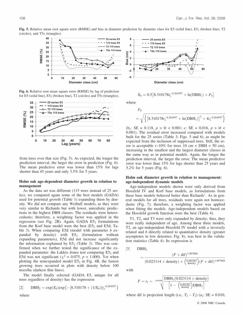
from trees over that size (Fig. 5). As expected, the longer theprediction interval, the larger the error in prediction (Fig. 6).The mean predictive error was lower than 15% for lagsshorter than 45 years and only 3.5% for 5 years.

Holm oak age-dependent diameter growth in relation tomanagement

As the data set was different (115 trees instead of 25 ser-ies), we compared again some of the best models (GADA)used for potential growth (Table 1) expanding them by den-sity. We did not compare any Weibull models, as they werevery similar to Richards but with lower, unrealistic predic-tions in the highest DBH classes. The residuals were hetero-cedastic; therefore, a weighting factor was applied in theregression (see Fig. 2B). Again, GADA E52 formulationsfrom the Korf base model were the best (E52 and E5d; Ta-ble 3). When comparing E5d (model with parameter b ex-panded by density) with E52 (formulation withoutexpanding parameters), E5d did not increase significantlythe information explained by E52 (Table 3). This was con-firmed when we further tested the significance of the ex-panded parameter: the Lakkis–Jones test comparing E52 andE5d was not significant (�2 = 0.075, p = 1.000). Yet whenplotting the nonexpanded model E52 in Fig. 4B, the fastestgrowing trees occurred in plots with density below 100trees/ha (darkest thin lines).

The model finally selected (GADA E5, unique for alltrees regardless of density) has the expression

½2� DBH2 ¼ expðX0Þexp �½8:310178þ ð1=X0Þ�t�0:2645972

� where

X0 ¼ 0:5 8:310178t�0:2645971 þ lnðDBH1Þ þ F0

� where

F0

¼ffiffiffiffiffiffiffiffiffiffiffiffiffiffiffiffiffiffiffiffiffiffiffiffiffiffiffiffiffiffiffiffiffiffiffiffiffiffiffiffiffiffiffiffiffiffiffiffiffiffiffiffiffiffiffiffiffiffiffiffiffiffiffiffiffiffiffiffiffiffiffiffiffiffiffiffiffiffiffiffiffiffiffiffiffiffiffiffiffiffiffiffiffiffiffiffiffiffi

8:310178t�0:2645971 þ lnðDBH1Þ

� 2 þ 4t�0:2645971

n or

(b1: SE = 0.118, p > |t| < 0.001; c: SE = 0.016, p > |t| <0.001). The residual error increased compared with modelsbuilt for the 25 series (Table 3; Figs. 5 and 6), as might beexpected from the inclusion of suppressed trees. Still, the er-ror is acceptable (~10% for trees 10 cm < DBH < 50 cm),increasing in the smallest and the largest diameter classes inthe same way as in potential models. Again, the longer theprediction interval, the larger the error. The mean predictiveerror was lower than 15% for lags shorter than 25 years and5.2% for 5 years (Fig. 6).

Holm oak diameter growth in relation to management:age-independent dynamic models

Age-independent models shown were only derived fromHossfeld IV and Korf base models, as formulations fromthese base models behaved better than Richards’. As in gen-eral models for all trees, residuals were again not homoce-dastic (Fig. 7); therefore, a weighting factor was appliedwhen fitting the models. Age-independent models based onthe Hossfeld growth function were the best (Table 4).

T1, T2, and T3 were only expanded by density; thus, theywere really independent of age. Among these three models,T2, an age-independent Hossfeld IV model with a inverselyrelated and b directly related to quantitative density (greaterasymptotes in low densities; Fig. 8), was best in the valida-tion statistics (Table 4). Its expression is

½3� DBH2

¼ ðF þ difÞ1:007868

ð0:023114� densityÞ þ 0:465367density

� �ðF þ difÞ1:007868

with

F ¼ t1 ¼ffiffiffiffiffiffiffiffiffiffiffiffiffiffiffiffiffiffiffiffiffiffiffiffiffiffiffiffiffiffiffiffiffiffiffiffiffiffiffiffiffiffiffiffiffiffiffiffiffiffiffiffiffiffiDBH1ð0:023114� densityÞ

1� 0:465367density

� �DBH1

h i1:007868

vuut

where dif is projection length (i.e., T2 – T1) (a1: SE = 0.010,

Fig. 5. Relative mean root square error (RMSE) and bias in diameter prediction by diameter class for E5 (solid line), E52 (broken line), T2(circles), and T5s (triangles).

Fig. 6. Relative root mean square error (RMSE) by lag of predictionfor E5 (solid line), E52 (broken line), T2 (circles) and T5s (triangles).

108 Can. J. For. Res. Vol. 38, 2008

# 2008 NRC Canada

p > |t| < 0.001; b1: SE = 0.001, p > |t| < 0.001; c: SE =0.088, p > |t| < 0.001). Contrary to GADA age-dependentmodels, age-independent models only expanded by densitywere slightly biased in the validation phase, and theirRMSE increased 80% as compared with the age-dependentmodels (Table 4). In Figs. 5 and 6, the relationship betweenthe predicted errors and diameter class or lag of intervalprediction are shown: the lag interval below 15% error was20 years, the error increasing as usual with lag length.

When expanding the age-independent formulations also

by site index, the error greatly decreased compared withreal age-independent models T1, T2, and T3. In addition,models T4s and T5s were almost unbiased (Table 4; Figs. 5and 6). The inclusion of the site index reduced in T5s themean residual by 17% and the mean bias to around 75%compared with age-independent T2. The lag of predictionwith error below 15% increased to 25 years (Fig. 6). Themodel (T5s) expression is

½4� DBH2 ¼ðF þ difÞ0:859611

ð 0:002797� densityþ 31:4296=SIÞ þ �0:06588density

� �þ 0:000123� SI

h iðF þ difÞ0:859611

with

F ¼ffiffiffiffiffiffiffiffiffiffiffiffiffiffiffiffiffiffiffiffiffiffiffiffiffiffiffiffiffiffiffiffiffiffiffiffiffiffiffiffiffiffiffiffiffiffiffiffiffiffiffiffiffiffiffiffiffiffiffiffiffiffiffiffiffiffiffiffiffiffiffiffiffiffiffiffiffiffiffiffiffiffiffiffiffiffiffiDBH1 � ð0:002797� densityþ 31:4296=SIÞ1� �0:06588

density

� �þ 0:000123� SI

h iDBH1

n o0:859611

vuut

where dif is projection length and SI is site index in cm (a1:SE = 0.000, p > |t| < 0.001; ad1: SE = 0.0275, p > |t| < 0.017;b1: SE = 1.426, p > |t| < 0.001; bd1: SE = 0.000, p > |t| <0.001; c: SE = 0.0084, p > |t| < 0.001). Both models 3 and4 are polymorphic and with variable asymptotes for differentdensities and site indexes (Fig. 8).

Discussion

This study is the first attempt to model diameter growth inholm oak tree like woodlands. Fitting growth models to thisspecies in this ecosystem is challenging for its particular man-agement and uncertain history. Despite the versatility of thespecies to thrive in a variety of climates and soils, the historicalisolation of tree formations to marginal soils has probably re-duced the presence of the species to the worst soil conditions.Nevertheless, it is very likely that trees analyzed exhibit nearmaximal growth for holm oak in this area, as humans, whoprobably selected the best trees, enforced the current struc-ture, with low tree densities. Holm oak has been traditionallyconsidered a slow-growth species (Ibanez et al. 1999). In ourresults, mean growth is slightly slower than that of otherMediterranean oaks such as Q. suber (Sanchez-Gonzalez etal. 2005; Tome et al. 2006) and Quercus pyrenaica Willd.

(Adame et al. 2007). Diameter growth is expected to begreater in low-density agroforestry systems than in forests(Balandier and Dupraz 1999). The young age range foundin this study, and in other analyzed samples not includedhere (partly described in Plieninger et al. 2003), where themaximum age was also below 200 years, agree with thehypothesis that most dehesas originated since the earlynineteenth century, mostly after the 1850s and the firsthalf of the twentieth century (Manuel and Gil 1999; Pulidoet al. 2001; Martın Vicente and Fernandez Ales 2006).

Formulations derived from power decline base models(Korf and Hossfeld) rather than exponential decline (Ri-chards, Weibull when c > 1 (Kiviste et al. 2002)) best de-scribed diameter growth in all cases, as stated in theliterature (Zeide 1989, 1993; Shvets and Zeide 1996). Theanalysis of ‘‘potential growth’’ describes how species growand provides tools that can be applied in system models(Porte and Bartelink 2002). What we consider here as ‘‘po-tential growth’’ could be more accurately denominated‘‘maximum diameter growth under traditional ‘dehesa’ man-agement’’. As in other previous studies, GADA formulationshad a slightly better fit than simpler ADA (e.g., Cieszewski2002; Barrio-Anta et al. 2006). The model selected (E5),polymorphic and with variable asymptotes GADA formula-

Table 3. Parameter estimates and goodness-of-fit statistics for the age-dependent models for 115trees (parameters expanded and nonexpanded by density).


ID RMSE (cm) R2 AICd MBias (cm) RMSE (cm) EF AICdE32 0.7234 0.9926 8.5 0.0670 2.6532 0.9508 89.2E52 0.7217 0.9927 0.0 –0.0492 2.5887 0.9532 0.0E92 0.7327 0.9924 54.4 0.0827 3.0584 0.9347 603.3E3d 0.7234 0.9926 10.3 0.0767 2.6787 0.9499 122.7E5d 0.7217 0.9927 1.7 –0.0386 2.6031 0.9527 19.1

Note: Estimation statistics were calculated using the weighted residuals. In E3d, b = (b1+ bd � density)X; inE5d, b = (b1+ bd � density) + (1/X).


# 2008 NRC Canada

tion derived from the Korf growth function, fit the data witha reduced RMSE of 2.6 cm and 7% in DBH classes from 10to 45, coinciding with the diameter range within which mosttrees of the dehesas are found (Pulido et al. 2001). The er-rors yielded (Tables 2–4; Figs. 5 and 6) are in accordancewith site dynamic growth studies for other tree species(e.g., Barrio-Anta et al. 2006; Dieguez-Aranda et al. 2006).

The wide range of densities included in our plots makespossible the comparison between ‘‘potential models’’ andthe effect of density in general models for all trees regard-less of their social position within the stand. Although den-sity was not included in the models, the most open standscoincided with the most productive (Fig. 4B); the reasoncould be that humans thinned the most productive sitesmore intensively, and in turn, this has produced better pas-tures. Thus, the positive effect of low density and fertilesites is likely to be combined in these anthropic woodlands.The small increase in the error with respect to ‘‘potentialgrowth’’ models and the similarity between the model for25 series and the model for 115 trees would support the hy-pothesis of codominance of most trees. This could havebeen expected, as only 23.5% of trees had been considered‘‘suppressed’’ in the graphical analysis, meaning that thefive trees analyzed per plot generally exhibited very similargrowth. Our results support the use of a single model for alldensities and for any tree in the system, as the error does notincrease significantly. An average tree would reach ~15 cmDBH after 30 years, which is in accordance with the approx-imate age suggested for cattle exclusion on regenerated sites(San Miguel 1994). This mean tree would reach around27 cm at 60 years and 35 cm at 90 years (see Fig. 4B).

Model 2 can be applied to any tree in the system withoutdefining dominance. However, accurately estimating treeage in holm oak is extremely difficult. This is the reasonwhy we compared age-independent formulations (Tome etal. 2006) with the previous age-dependent dynamic models.When expanding only by density, the models where slightlybiased and increased the error except in prediction lagsgreater than 50–60 years, where age-independent modelswere better. Yet this increase was acceptable, especiallybearing in mind the advantage of neglecting age. Addition-ally, the highest errors in models 3 and 4 coincided withthe smallest and greatest diameter classes. This is a normalfeature in growth models that results from a lack of data in

the largest classes and worse predictive ability in the young-est ages. When expanding also by site index (model 4), theerror significantly decreased, with a behaviour similar tothat of the general age-dependent model 2, especially whenanalyzing the mean error by lag of prediction. In both mod-els, the smallest error was again centred in diameter classesfrom 20 to 50 cm (Fig. 5), which are the most abundant inthe system today (Pulido et al. 2001). In T5s, density ex-plained less variance than site index, which is in accordancewith the noninclusion of density in E52. Although T5s is nottotally ‘‘age independent’’, as site index must be estimated,it enabled us to test the validity of the defined site indexand compare our results with those of Tome et al.’s (2006)original paper. The aforementioned increase in error with re-spect to age-dependent dynamic models found in our analy-sis is not totally compatible with the results of Tome et al.(2006) for Q. suber age-independent formulations in a simi-lar system. In that study, age-independent models had aslight better fit than age-dependent ones. Nevertheless, weconsider our results reasonable: when significant covariatesare added to an equation (‘‘age’’ in this case), the error islikely to decrease and the goodness-of-fit increase. In addi-tion, T5s would likely improve if soil and climatic datawere available. Although we believe that it is unlikely to ex-plain such a great difference in the increase in error with re-spect to that study, the increase in error found in our modelsmight result from the use of a site index derived from diam-eter rather than from height. Acknowledging the previousshortcomings and from the tremendous advantage of ne-glecting age, we believe that the error yielded is acceptablein the middle diameter classes, which are the most commonin these woodlands, as discussed. Age-independent modelsare an alternative to model growth in tree species that donot form annual rings, including many species in the tropics(Verheyden et al. 2005), and can be applied to other agro-forestry systems, particularly in Mediterranean climates(e.g., Jackson et al. 1990; Ovalle et al. 1990), and touneven-aged stands (Tome et al. 2006).

The site index based on diameter growth proposed wassignificant in T5s. This would support the definition of siteindexes based on diameter growth in open stands. It is sup-ported by an ecological basis, if we accept that when cano-pies are competing for light, trees tend to focus growth inheight, whereas isolated trees focus growth in increasingtheir canopies and stem diameter (Hasenauer 1997). There-fore, in open stands, we could consider diameter growth aspotential at least in terms of competition for light. Finally,the fact that current density was included in age-independentlife-span models might reflect the human influence uponthese systems: the current woodland structure and densitywere modified decades ago and the stands are static exceptfor tree death, which is gradually reducing the tree stock.

In this study, we offer different possibilities to model diam-eter growth in holm oak open woodlands. It would be inter-esting to study the difference comparing the implementationof a site index based on a general equation for all treeswith a site index based on potential growth series, particu-larly when soil and climate variables are available.Whether these models, based on past growth, are appropri-ate to predict diameter under different future climatic sce-narios is something that should be studied.

y = -0.1986 ln(x) + 1.0923R2 = 0.7864

0

0.2

0.4

0.6

0.8

1.0

0 15 30 45 60 75DBH (cm)

Var

ian

ce r

esid

ual

sFig. 7. Estimation residuals (predicted-observed) versus predictedDBH as an illustration of potential heterokedasticity for age inde-pendent formulations. Residual variance by diameter class and esti-mated variance function (i.e., weigth, wi) applied in T2 and T5s.

110 Can. J. For. Res. Vol. 38, 2008

# 2008 NRC Canada

ConclusionsThe ‘‘potential growth’’ equations were unbiased and with

an error of around 7% in the most abundant diameter classesencountered in the system, modelling the data and theasymptotic growth tendency of the species very well. Thegeneral age-dependent model selected, applicable to anytree within any stand density knowing its age, did not in-crease the error (which was around 10% in DBH from 10 to50 cm) much compared with the ‘‘potential’’ models. Den-sity did not provide much information in the age-dependentmodels, whereas in age-independent models, in spite ofbeing significant, the residual errors decreased when the siteindex proposed was used to expand the parameters. The in-clusion of the defined site index in the models increased theaccuracy of age-independent formulations, although it addedthe same limitation that age must be estimated to define thesite index. Age-independent models including site indexwere similar to general age-dependent models in the mostabundant diameter classes in the system (20–55 cm). Thediscussion of age-independent dynamic models offers man-agers and researchers of other agroforestry systems and trop-ical forests new alternatives for modelling dynamic growthin highly altered tree systems and in species or stands wherethe determination of age is cumbersome.

AcknowledgementsWe gratefully acknowledge Enrique Garriga for thor-

oughly processing the samples. Rafael Alonso, Marcos Bar-rio, Rafael Calama, Darıo Martın-Benito, and MariolaSanchez-Gonzalez greatly helped with discussion. LourdesCruz and PyG made possible the access to the study area

and collection of the samples. The authors are indebted totwo anonymous reviewers whose suggestions greatly im-proved the manuscript.

ReferencesAdame, P., Hynynen, J., Canellas, I., and del Rıo, M. 2007. Indivi-

dual tree-diameter growth model for rebollo oak (Quercus pyre-naica Willd.) coppices. For. Ecol. Manag. In press. doi:101016/j.foreco.2007.10.1019.

Alvarez, J.G., Barrio, M., Dieguez, U., and Rojo, A. 2004. Metodo-logıa para la construccion de curvas de calidad de estacion. Cua-dernos de la SECF No. 18. pp. 303–309.

Ares, A., and Brauer, D. 2004. Growth and nut production of blackwalnut in relation to site, tree type and stand conditions insouth-central United States. Agrofor. Syst. 63: 83–90.

Bailey, R.L., and Clutter, J.L. 1974. Base-age invariant poly-morphic site curves. For. Sci. 20: 155–159.

Balandier, P., and Dupraz, C. 1999. Growth of widely spaced trees.A case study from young agroforestry plantations in France.Agrofor. Syst. 43: 151–167.

Barbero, M., Loisel, R., and Quezel, P. 1992. Biogeography, ecol-ogy and history of Mediterranean Quercus ilex ecosystems. Ve-getatio, 99–100: 19–34. doi:10.1007/BF00118207.

Barrio-Anta, M., Dorado, F.C., Dieguez-Aranda, U., AlvarezGonzAlez, J.G., Parresol, B.R., and Rodrıguez-Soalleiro, R.2006. Development of a basal area growth system for maritimepine in northwestern Spain using the generalized algebraic dif-ference approach. Can. J. For. Res. 36: 1461–1474. doi:10.1139/X06-028.

Burnham, K.P., and Anderson, D.R. 2004. Multimodel inference —understanding AIC and BIC in model selection. Sociol. MethodsRes. 33: 261–304. doi:10.1177/0049124104268644.

Fig. 8. Age independent models: (A) T2 for densities 55, 111 and 175 trees/ha; (B) T5s for site index 50 (Class I) and 23 (Class IV),densities 55 and 175 trees/ha.

Table 4. Age-independent holm oak diameter growth dynamic models with parameters expanded bystand density (T1, T2, and T3) and (or) site index (T4s and T5s).


ID RMSE (cm) R2 AICd MBias (cm) RMSE (cm) EF AICdT1 0.6762 0.9927 900.0 –0.4007 4.7340 0.8333 6240.8T2 0.6781 0.9927 981.2 –0.5587 4.6274 0.8407 5549.2T3 0.6856 0.9925 1317.7 –0.4495 4.7475 0.8323 6327.3T4s 0.6632 0.9930 307.7 –0.0742 4.0366 0.8788 1400.5T5s 0.6565 0.9931 0.0 –0.1413 3.8545 0.8895 0.0

Note: Estimation statistics were calculated using the weighted residuals.


# 2008 NRC Canada

Carmean, W.H. 1975. Forest site quality evaluation in the UnitedStates. Adv. Agron. 27: 209–269.

Cherubini, P., Gartner, B.L., Tognetti, R., Braker, O.U., Schoch, W.,and Innes, J.L. 2003. Identification, measurement and interpreta-tion of tree rings in woody species from mediterranean climates.Biol. Rev. 78: 119–148. doi:10.1017/S1464793102006000.PMID:12620063.

Cieszewski, C.J. 2002. Comparing fixed- and variable-base-age siteequations having single versus multiple asymptotes. For. Sci. 48:7–23.

Cieszewski, C.J. 2003. Developing a well-behaved dynamic siteequation using a modified Hossfeld IV function Y3 = (axm)/(c +xm–1), a simplified mixed-model and scant subalpine fir data.For. Sci. 49: 539–554.

Cieszewski, C. 2004. GADA derivation of dynamic site equationswith polymorphism and variable asymptotes from Richards,Weibull, and other exponential functions. Daniel B. WarnellSchool of Forest Resources, University of Georgia, Athens, Ga.

Cieszewski, C., and Bailey, R.L. 2000. Generalized algebraic dif-ference approach: theory based derivation of dynamic site equa-tions with polymorphism and variable asymptotes. For. Sci. 46:116–126.

Cieszewski, C., Harrison, M., and Martin, S. 2000. Practical meth-ods for estimating non-biased parameters in self-referencinggrowth and yield models. Daniel B. Warnell School of ForestResources, University of Georgia., Athens, Ga.

Cieszewski, C.J., Zasada, M., and Strub, M. 2006. Analysis of dif-ferent base models and methods of site model derivation forScots pine. For. Sci. 52: 187–197.

DGB. 1999. Segundo IFN 1986–1996. Ministerio de Medio Am-biente, Madrid.

Dieguez-Aranda, U., Burkhart, H.E., and Amateis, R.L. 2006. Dy-namic site model for loblolly pine (Pinus taeda L.) plantationsin the United States. For. Sci. 52: 262–272.

Fritts, H.C. 1976. Tree rings and climate. Blackburn Press, Cald-well, N.J.

Garcıa del Barrio, J.M., Bolanos, F., Ortega, M., and Elena-Ros-sello, R. 2004. Dynamics of land use and land cover change indehesa landsapes of the ‘REDPARES’ network between 1956and 1998. Adv. Geoecol. 37: 47–54.

Gene, C., Espelta, J.M., Gracia, M., and Retana, J. 1993. Identifica-cion de los anillos anuales de crecimiento de la encina (Quercusilex L.). Orsis Org. Sist. 8: 127–139.

Goelz, J.C.G., and Burk, T.E. 1992. Development of a well-be-haved site index equation: jack pine in north central Ontario.Can. J. For. Res. 22: 776–784.

Gomez, J.M., and Perez, M. 1996. The ‘dehesas’: silvopastoral sys-tems in semiarid Mediterranean regions with poor soils, seasonalclimate and extensive utilisation. In Western European silvopas-toral systems. Edited by M. Etienne. INRA, Paris. pp. 55–70.

Hasenauer, H. 1997. Dimensional relationships of open-grown treesin Austria. For. Ecol. Manag. 96: 197–206. doi:10.1016/S0378-1127(97)00057-1.

Ibanez, J.J., Lledo, M.J., Sanchez, J.R., and Roda, F. 1999. Standstructure, aboveground biomasa and production. In Ecology ofMediterranean evergreen oak forests. Springer, Berlin. pp. 31–45.

Jackson, L.E., Strauss, R.B., Firestone, M.K., and Bartolome, J.W.1990. Influence of tree canopies on grassland productivity andnitrogen dynamics in deciduous oak savanna. Agric. Ecosyst.Environ. 32: 89–105.

Khattree, R., and Naik, D.N. 1995. Applied multivariate statisticswith SAS software. SAS Institute Inc., Cary, N.C.

Kiviste, A., Alvarez Gonzalez, J.G., Rojo Alboreca, A., and RuizGonzalez, A.D. 2002. Funciones de crecimiento de aplicaciones

en el ambito forestal. Ministerio de Ciencia y Tecnologıa, INIA,Madrid.

Kozak, A., and Kozak, R. 2003. Does cross validation provide ad-ditional information in the evaluation of regression models?Can. J. For. Res. 33: 976–987. doi:10.1139/x03-022.

Lundqvist, B. 1957. On the height growth in cultivated stands ofpine and spruce in northern Sweden. Medd. Fran Statens Skog-forskningsinstitut. 47(2).

Manuel, C., and Gil, L. 1999. La transformacion historica del pai-saje forestal en Espana. In Segundo IFN 1986–1996. Ministeriode Medio Ambiente, Madrid. pp. 15–104.

Martın-Vicente, A., and Fernandez-Ales, R. 2006. Long term per-sistence of dehesas. Evidences from history. Agrofor. Syst. 67:19–28. doi:10.1007/s10457-005-1110-8.

Mosquera, M.R., McAdam, J., and Rigueiro, A. (Editors). 2005.Silvopastoralism and sustainable land management. CAB Inter-national, Wallingford, U.K.

Myers, R.H. 1990. Classical and modern regression with applica-tions. 2nd ed. Duxbury Press, Belmont, Calif.

Ovalle, C., Aronson, J., Del Pozo, A., and Avendano, J. 1990. Theespinal: agroforestry systems of the mediterranean-type climateregion of Chile. Agrofor. Syst. 10: 213–239. doi:10.1007/BF00122913.

Peschel, W. 1938. Mathematical methods for growth studies oftrees and forest stands and the results of their application. Thar-andter Forstliches Jahrburch, 89: 169–247. [In German.]

Plieninger, T., Pulido, F.J., and Konold, W. 2003. Effects of land-use history on size structure of holm oak stands in Spanish de-hesas: implications for conservation and restoration. Environ.Conserv. 30: 61–70.

Porte, A., and Bartelink, H.H. 2002. Modelling mixed forestgrowth: a review of models for forest management. Ecol.Model. 150: 141–188. doi:10.1016/S0304-3800(01)00476-8.

Pulido, F.J., and Dıaz, M. 2005. Regeneration of a Mediterraneanoak: a whole-cycle approach. Ecoscience, 12: 92–102. doi:10.2980/i1195-6860-12-1-92.1.

Pulido, F.J., Dıaz, M., and Hidalgo de Trucios, S.J. 2001. Sizestructure and regeneration of Spanish holm oak Quercus ilexforests and dehesas: effects of agroforestry use on their long-term sustainability. For. Ecol. Manag. 146: 1–13. doi:10.1016/S0378-1127(00)00443-6.

Richards, F.J. 1959. A flexible growth function for empirical use.J. Exp. Bot. 10: 290–300. doi:10.1093/jxb/10.2.290.

Rinntech. 2003. TSAP-WIN. Time series analysis and presentationfor dendrochronology and related applications. Version 0.53.Rinntech, Heidelberg, Germany.

Roda, R., Retana, J., Gracia, C.A., and Bellot, J. (Editors). 1999.Ecology of Mediterranean evergreen oak forests. Springer-Verlag, Berlin.

San Miguel, A. 1994 La dehesa espanola: origen, tipologıa, carac-terısticas y gestion. Fundacion Conde del Valle de Salazar,Madrid.

Sanchez-Gonzalez, M., Tome, M., and Montero, G. 2005. Model-ling height and diameter growth of dominant cork oak trees inSpain. Ann. For. Sci. 62: 633–643. doi:10.1051/forest:2005065.

SAS Institute Inc. 2004. SAS/ETS 9.1 user’s guide. SAS InstituteInc., Cary, N.C.

Shvets, V., and Zeide, B. 1996. Investigating parameters of growthequations. Can. J. For. Res. 26: 1980–1990.

Tome, J., Tome, M., Barreiro, S., and Amaral Paulo, J. 2006.Age-independent difference equations for modelling tree andstand growth. Can. J. For. Res. 36: 1621–1630. doi:10.1139/X06-065.

Verheyden, A., De Ridder, F., Schmitz, N., Beeckman, H., and

112 Can. J. For. Res. Vol. 38, 2008

# 2008 NRC Canada

Koedam, N. 2005. High-resolution time series of vessel densityin Kenyan mangrove trees reveal a link with climate. New Phy-tol. 167: 425–435. doi:10.1111/j.1469-8137.2005.01415.x.PMID:15998396.

von Bertalanffy, L. 1957. Quantitative laws in metabolism andgrowth. Q. Rev. Biol. 32: 217–231. PMID:13485376.

Weibull, W. 1951. A statistical distribution function of wide ap-plicability. J. Appl. Mech. 18: 293–297.

Yang, R.C., Kozak, A., and Smith, J.H.G. 1978. The potential of

Weibull-type functions as flexible growth curves. Can. J. For.Res. 8: 424–431.

Zeide, B. 1989. Accuracy of equations describing diameter growth.Can. J. For. Res. 19: 1283–1286.

Zeide, B. 1993. Analysis of growth equations. For. Sci. 39: 594–616.

Zhang, S.H., and Romane, F. 1991. Variations de la croissance ra-diale de Quercus ilex L. en fonction du climat. Ann. Sci. For.48: 225–234.


# 2008 NRC Canada

site index in agroforestry systems: age-dependent and age

Documents