i

PREDICTION OF PROCESS-INDUCED DEFECTS BY PLY-DROPS IN THE DESIGN

OPTIMIZATION OF A COMPLEX COMPOSITE LAMINATE.

by

SITANSHU PANDYA

Presented to the Faculty of the Graduate School of

The University of Texas at Arlington in Partial Fulfillment

of the Requirements

for the Degree of

Master of Science in Mechanical Engineering

THE UNIVERSITY OF TEXAS AT ARLINGTON

August 2017

ii

Copyright © by Sitanshu Pandya 2017

All Rights Reserved

iii

ACKNOWLEDGEMENTS

I would like to express my gratitude towards my supervising professor Dr. Robert

M. Taylor, his invaluable support, endless guidance with patience, and motivation made

this thesis study possible. I would like to thank Dr. Alex Selvarathinam and Dr. Scott

Norwood and for their remarks and guidelines on this work. I express my gratitude to Dr.

Wen S. Chan providing material and advice.

Additionally, I would like to thank Dr WOODS, Scott Berggen, and Anirudh Jayan

for support in manufacturing and Jo Novak and Blesson Isaac for helped me in MATLAB

coding part.

August 3, 2017

iv

DEDICATION

This thesis study is dedicated to Guru Shivanandji and my parents Mr. Harkantray

D Pandya and Mrs. Devyani H Pandya, for their unconditional love and support throughout

my life.

I would appreciate Deepak Polaki’s efforts for guiding and explaining concepts and

procedure throughout my research work. I also would like to thank Sanjana Shah, my

brothers Chinmay Godbole, Piyush Yadav and Pritish Mandre and many others for their

encouragement throughout my academic life.

July 11, 2017

v

ABSTRACT

Prediction of Manufacturing Defects during Cure Process Induced by

Ply-Drops in the Design Optimization of Complex Composite Laminate.

Sitanshu Pandya, MS

The University of Texas at Arlington, 2017

Supervising Professor: Robert M. Taylor

The objective of this work is to characterize manufacturing process-induced warping

defects due to ply drops in composite laminates to guide composite laminate design.

Composite laminate optimization seeks weight efficient models, but the process can also

generate complex ply geometry, which compounds the challenges of the already rigorous

composite laminate manufacturing process. Increased design complexity enhances the

likelihood of manufacturing process-induced defects like warping; therefore, it is important

to predict such defects in the design phase to make the product more efficient yet

producible and thereby avoid such defects. This work study is manufacturing process-

induced warpage in complex composite laminates from a three-phase design optimization

process that includes composite free size conceptual design ply sizing optimization, and

stacking sequence optimization. A mathematical model that could be included in

optimization process could help eliminate these defects in the design phase. Consequently,

an Analytical model was developed to predict warpage and was compared with

experimental and finite element models. The full-size optimized laminate was fabricated,

to understand the manufacturing defects for an actual composite laminate. The results

obtained from the analytical model correlated with the results of experimental and finite

element models. Hence, the mathematical model could be incorporated into the three-

phase optimization process.

vi

TABLE OF CONTENTS

Acknowledges………………………………………………………………………………….…iii

Dedication…………………………………………………………………………………………iv Abstract ............................................................................................................................... v

List of Illustrations ............................................................................................................. viii

List of Tables ....................................................................................................................... x

CHAPTER 1: INTRODUCTION…………………….……………........................................11

CHAPTER 2: BACKGROUND……………………………………………..……………..……12

2.1 Design Optimization……………………………………………………..……12

2.2.1 Composite Free Size optimization (ply shape optimization)………..13

2.2.2 Composite Size optimization……………………….……………..……13

2.2.3 Shuffling optimization…………………………………………………...14

2.2 Composite Laminate Manufacturing Processes……………………………15

2.3 Types of Defects Induced due to Manufacturing……………………………21

CHAPTER 3: COMPOSITE LAMINATE Design and Manufacturing Study……………....25

3.1 motivation/objective………………………………………………..……..…25

3.2 Free-size optimization on optimized composite laminate…………………25

3.2.1 Model formulation……………………………………………………...26

3.3 Size optimization on optimized composite laminate……………………….28

3.4 Shuffling optimization on optimized composite laminate………………....29

3.4.1 Buckling Criteria…………………………………………….………….29

3.4.2 Manufacturing Criteria………………………………………...……...29

3.4.3 Validation of stacking sequence………………………………….….30

vii

3.5 Editing Finite Element Model to CAD model……………….……….…….31

3.6 Manufacturing……………………………………………….………….…….34

3.7 Manufacturing induced defects…………………………………….……….38

CHAPTER 4: Warpage Prediction Models…………………………………………….……..39

4.1 Analytical Model for predicting Warpage due to

cooling cycle in cure process ………………………………….……….....39

4.2 Experimental model - Fabricating coupons ………….…………..….…..43

4.3 Finite Element Modal for predicting warpage due to

cooling cycle in cure process……....…………………………......……… 45

CHAPTER 5: Warpage Prediction Results ……………...……………………………….….49

5.1 Analytical Model for predicting Warpage due to

cooling cycle in cure process……………………………………………….…….49

5.2 Experimental model - Fabricating coupons……………………….………….…51

5.3 FEM modal for predicting Warpage due to

cooling cycle in cure process……………………………………….…….……. 54

5.4 Comparison Results…………………………………………………….….……..58

CHAPTER 6: CONCLUSION and FUTURE WORK……………………………….………..59

APPENDICES

A. FEM file structure for shuffling optimization…..............................................................61

B. MATLAB CODE………………………………………….………….……………...….…….69

C. FEM FILE STRUCTURE for Coupons……………….…………………………....………75

REFERENCES………………………………….……………..…………………………….….78

viii

LIST OF ILLUSTRATIONS

Figure 1: Three phase optimization process…………………………………………..……..12

Figure 2: Autoclave in composite lab, Mae dept., uta…………………………………...…..16

Figure 3: Oven with vacuum lines and thermocouple…………………………………...…..17

Figure 4: Compression heat molding machine, utari…………………………………..……18

Figure 5: Laminate geometry …………………….……………..………………………….….26

Figure 6: Ply-drop schematic……………………………………………………………….….30

Figure 7: Optimized stacking sequence……………………………………………………....30

Figure 8: Unedited ply shapes ………………………………………………………………..31

Figure 9: Hypermesh GUI command for ply smoothing and surface generation ………..32

Figure 10: Edited ply shapes ………………………………………………………………….33

Figure 11: Ply arrangement for cutting through nesting process ……………………...…..34

Figure 12: Ply cutting at 45° …………………………………………………………………...35

Figure 13: Ply shapes of carbon fiber tapes …………………………………………………35

Figure 14: Lay-up process, release film, and breather ……………………………………..36

Figure 15: Vacuum bagging …………………………………………………………………...37

Figure 16: Demo cure cycle of Hexcel im6/3506-1. ………………………………………...38

Figure 17: Cured laminate with warpage …………………………………………………….38

Figure 18(a): Actual ply-drop intersection FBD ……………………………….……………39

Figure 18(b): Modified ply-drop intersection FBD …………………………………………..39

Figure 19: Schematic of analytical model ……………………………………………………40

Figure 20 (a): Coupons before cure ………………………………………………………….44

Figure 20 (b): Coupons after cure …………………………………………………………….44

Figure 21: Coupons with restricted edges………………………………………...………….45

Figure 22: Boundary condition: Roller support at the end………………………………….48

ix

Figure 23: Command in HyperMesh for material orientation for 3d elements …………...48

Figure 24: Deformation results based on the analytical model for 0...…………….………49

Figure 25: Deformation results based on the analytical model for 90….………….……...50

Figure 26: Deformation results based on the analytical model for -/+45………….………50

Figure 27: Trends of change in angle of with ply-drops and the orientation

for Analytical model…………………………………………………………….…51

Figure 28: 0° Orientation layup with 16 ply-drop ………………………….……….….……52

Figure 29: -/+45° Orientation layup with 16 ply-drop ……………………………….….…..52

Figure 30: 90° Orientation layup with 16 ply-drop …………………………………..….…..52

Figure 31: coupling effect for a classical lamination theory…………………………..……53

Figure 32(a): Coupons with restricted edges after cure………..…………………….…….53

Figure 32 (b): Moment at ply-drop intersection……………………………………….……..54

Figure 33(a): 0° plies with 16 ply-drops …………………………………………….….……55

Figure 33(b): 0° plies with 16 ply-drops 100x exaggerated………………………….….…55

Figure 34(a): 90 plies with 16 ply-drops …………………………..……………..……....….56

Figure 34(b): 90° plies with 16 ply-drops 100x exaggerated ……………………….….….56

Figure 35(a): -/+45° plies with 16 ply-drops…………………………………………….…...57

Figure 35(b): -/+45° plies with 16 ply-drops 100x exaggerated ……………………….….57

Figure 36: Trends of change in angle of with ply-drops and the orientation for FEM…..58

Figure 37: Comparison of FEM and Analytical results………………………………….....59

Figure 38: Z-displacement for composite laminate after thermal loading…………….… 60

Figure 39: (a)Ply slope effect on larger panel (b) Ply drop effect on smaller panel….…60

Figure 40: Cross-sectional view of optimize composite plate………………………….….61

x

LIST OF TABLES

Table 1: List of consumables material used during hand layup process………………….18

Table 2 : Generic composite material properties………………………………………….…26

Table 3: Generic carbon fiber/epoxy tape material system maximum strain criterion

allowable………………………………………………………………………………27

Table 4: Generic carbon fiber/epoxy tape material system constant value bearing and

bypass Allowable……………………………………………………………………..28

Table 5: Material properties of IM6/3506-1 for analytical model………………….………..41

Table 6: Experimental model for different combination ply-drop and orientation………...43

Table 7: Experimental model for different combination ply-drop and

orientation with restricted edges…………………………………….….………….45

Table 8: FEM model for different combination ply-drop and orientation……………….….46

Table 9: Material properties for IM6/3506-1 prepreg………………………………….…….46

Table 10: Material properties for 3506-1 resin system………………………………………47

11

1. Introduction

Design and Manufacturing of composite structures have been a challenging and time-

consuming process. Composite structures are weight efficient when compared with other

engineering materials used in industries, but the cost is a major factor for using composites

structures. Therefore, there are a need for more efficient weight, and material saving

designs methods. Design Optimization is one of the ways to achieve this objective. As the

variation of material is bi-directional regarding mechanical properties of composites, the

optimization process is more complex with some possible design solutions out of which to

choose correct solutions, is complicated decision-making process by achieving all

objectives. Hence a new approach was developed by Altair suggested by Ming Zhou,

Raphael Fleury, and Martin Kemp2 which is cost saving and efficient for composite

structural optimization. This three-phase optimization process gives a weight efficient

design, but also the results have some complex ply geometry which makes manufacturing

more challenging, and the finished product would be unpredictable. In this thesis study, the

aim is to develop a mathematical model to include that in design optimization phase to

avoid this defect. Hence, an Analytical model was developed based on the classical

lamination theory for the ply-drop intersection, and the results were compared with

experimental and finite element model to validate the results from the analytical model. The

full-size composite laminate was fabricated. The uniqueness of this study is on the focus

on deformation of the complex composite laminate produced during cure process due to

series of ply-drops within the laminate.

12

2. Background

This thesis study is a continuation of “COMPOSITE PLATE OPTIMIZATION WITH

STRUCTURAL AND MANUFACTURING CONSTRAINTS by Deepak Polaki, supervised

by Dr. Robert Taylor. In continuation to this study shuffling optimization was performed on

the optimized composite laminate after free-size and size optimization. The laminate was

manufactured, and a detailed study of manufacturing induced defects due to uneven

thickness was carried out in this thesis. This section helps to relate and understand the

research done previously.

2.1 Design Optimization

Design optimization of the isotropic structure is simple compared to composite

structures optimization. As composites are heterogeneous, material properties vary in the

multiple-coordinate system and considering these changes; an optimization process has

to generate a best possible shape, size and stacking sequence for plies within composite

laminate18. Three phase optimizations of the composite structure are popular in the aircraft

industry. Phase I focuses on generating ply shapes through Free-Size optimization; Phase

II further improves the number of plies for a given ply layup and regulates the individual ply

thickness along with total laminate thickness: Then Phase III finalizes design details

through Stacking sequence optimization satisfying all manufacturing and design

constraints2.

2.1.1 Composite Free Size Optimization

Figure 1: Three phase optimization process2

13

In 2014, Taylor R. et al., considered a laminate with a rectangular cut out with one hole

with practical design constraints, studied, compared weights, and manufacturability

through various optimization methods27,28. Orthotropic composite structures require a

higher level of tooling and additional processes at the conceptual level. Design and

manufacturing constraints are implemented at the system level, and stacking sequence

optimization is applied at the detail level to formulate the final design of the structure.

2.1.1 Free Size Optimization

Free size optimization uses the thickness parameter as a size parameter and offers a

direct fix for the precision problem in the shell elements. Thus, creating topological- style

optimization result. However, this type is restricted to only isotropic materials; a generalized

process can be used for the composite materials.

This phase uses the outer boundary of the plies to modify the problem. Various grid

locations are allocated to the outer part of each ply based on applied loading conditions by

satisfying all constraints and achieving the objective to create optimal ply shapes. M.Pohlak

et al...30 and Polaki D1 have used free size optimization in a multi stage criteria optimization

of large plastic composite parts.

2.1.2 Composite Size Optimization

After topology/shape/free size optimization gives out the best possible shape, the size

optimization deals with attributes of elements such as shell thickness, beam cross-

sectional properties, spring stiffness, and mass. These attributes are redefined and

controlled according to design variable and constraints are satisfied during the optimization

process. In general, the objective is to minimize weight by optimizing elements along the

thickness and working on the overall thickness of the laminate. The variable thickness

could be possible depending on boundary condition with different load cases.

14

2.1.3 Shuffling Optimization

H Ghiasi, K Fayazbakhsh, D Pasini, L Lessard 19 developed optimization algorithms in

constant stiffness design. Different parameterization and optimization algorithms were

briefly explained and compared the advantages and shortcomings of each algorithm to get

optimal stacking sequence. Pagano, N. J., and R. Byron Pipes20 presented an approach

to predict the exact stacking sequence of specific orientations which leads which makes

design safe against delamination under uniaxial static and fatigue loadings.

The use of lamination parameters is another approach to represent the in-plane and

flexural stiffness in the optimization of laminated composites. Tsai first used the

optimization of composite laminate21 and later applied to the buckling optimization of

orthotropic laminated plates by Fukunaga, Hisao, and Hideki Sekine22 of laminated

composites.

The composite shuffling optimization step of the three-phase composite design

optimization determines optimal stacking of the plies to meet manufacturing requirements.

It is important to understand stacking sequence in a composite laminate product.

Though the design achieved after Phase II optimization contained all ply layout,

specific manufacturing constraints are not satisfied. Therefore, stacking sequence of

individual plies is being shuffled during this period to satisfy production constraints while

keeping all design constraints intact.

Some other manufacturing constraints are enforced: (a) limit on consecutive plies

of the same orientation (b) pre-defined cover lay-ups; (c) pre-defined core lay-ups.

15

2.2 Composite Laminate Manufacturing Process

The manufacturing process involves adding reinforcements to the resin system

which could be a final form of product or need to be prepared for the final product. Process

and tooling affect composite properties. Therefore, detailed knowledge of manufacturing is

required when designing composite parts.

There are two parts involved in manufacturing composite laminates: lay-up and

curing. The various process by are known for manufacturing as explained below:

1. Hand layup

The traditional and most commonly known technique is laying up composite plies

into the mold by hand. This method is used where there is less accuracy required.

It's labor intensive and time-consuming, but hand layup can eliminate the initial

cost and maintenance cost of complex machinery needed in a technique like ATP

and AFP.

a. Wet layup

In this type of process both resin and fiber are separate. Fibers are in the form

of dry fabric or unidirectional tapes or strands. The resin used in this kind of

process is two part epoxy thermoset resin. The first layer of resin is coated on

mold, fibers are placed, and successive layers of fiber and resin are coated on

one another. The number of layers of fiber are based on design. At the end

the layup, part is subjected to the curing process.

b. Prepreg Layup

Fibers are pre-impregnated with a resin system. This type of prepreg fibers

lay-up could be done directly on mold and could be subjected to the curing

process.

16

The curing process depends on resin system used in manufacturing. It involves vacuum,

high pressure, and temperature, and following are some common methods used for the

curing process:

a. Autoclave

The most common method used in the curing process is an autoclave, which is a

pressure vessel chamber that has a heating system and can hold vacuum as

shown in the picture below. The size of the autoclave, the range of temperature,

and pressure can operate on the curing system of resin which varies from

application to application.

b. Out of Autoclave

This process is used when there is no pressure, or little amount of pressure is

required to cure the resin system. A typical heat Oven with thermocouple and

vacuum lines could be used for this process. This type of curing is less accurate

Figure 2: AUTOCLAVE in COMPOSITE LAB, MAE dept., UTA

17

and can affect the final strength of the material. LW Davies, RJ Day, D Bond, A

Nesbitt, J Elli23 presented a cure cycle study, an out-of-autoclave toughened resin

film infusion process as part of the examination of an alternative manufacturing

process for composites. They showed that cure cycles with a relatively short dwell

time and higher heating rate compared to an autoclave cure led to enhanced flow

properties of the toughened resin system. High-quality laminates, comparable to

autoclave panels, were manufactured with vacuum pressure only by modifying the

original vacuum bagging arrangement.

c. Compression heat molding.

This type of curing is used where high temperature curing systems are required

like curing amide based resin or ceramic based composites. The heat is supplied

from two hot plates with a sealed chamber to hold vacuum and pressure is applied

by controlling compression between the plates. There is enormous initial and

maintenance cost involved with this kind of process, but it gives accurate results.

Figure 3: Oven with vacuum lines and thermocouple, IPPM, UTARI

18

The limitation with this process is it can only cure flat laminates with even

thickness.

Hand lay-up and curing is done, certain consumable materials are required throughout the

process. The following table explains each term and its uses:

Peel-ply A sacrificial open weave fiberglass or perforated heat-set nylon ply

placed between the laminate and the bleeder/breather to provide

the textured and clean surface necessary for further lamination or

secondary bonding.

Breather

cloth

The fiber volume fraction, and hence mechanical properties, can be

improved by bleeding off excess resin. To achieve this, a polymeric

film sealed to the mold edges encloses the laminate. A porous

material used to provide a gas flow path over the laminate both to

permit the escape of air, reactants, moisture, and volatiles and to

Figure 4: compression heat molding machine, IPPM, UTARI

19

ensure uniform vacuum pressure across the component. It may

also act as the bleeder cloth.

Release

film

A (perforated) sheet of material placed between the laminate and

the mold surfaces to prevent adhesion.

Caul

plate

A mold or tool set on top of the laminate inside the bag to define the

second surface.

Bagging

film

The plastic film which can hold vacuum within the bag.

Tacky

tape

Adhesive strip used to bond the bag to the tool and provide a

vacuum seal.

Breach

unit

A connector through the bagging film to permit a vacuum to be

drawn.

Vacuum

pipes

The link between the breach unit and the vacuum pump.

Vacuum

pump

A high-volume pump (absolute vacuum is rarely required) suitable

for continuous running. For some slow-curing epoxy resins, twenty-

four operation may be needed.

Pressure

gauges

Clock-type or digital gauges attached via a breach unit connection.

Vacuum

bagging

A breach unit penetrates the bag and permit a vacuum to be drawn

in the bag. This imposes a consolidation pressure of up to ~1000

mbar on the materials in the bag. The principal disadvantage of this

technique is the disposable materials that are included in the bag

Table 1: List of consumables material used during hand layup process32,33

20

2. Automatic Tape Placement(ATL):

The fabrication from ATL will be best suited for lay-up of complex ply shapes. ATL

systems were conceived from the end of the 1960s onwards8. The earliest known

reference to an ATL is a patent under the name of Chitwood and Howeth9 in 1971,

describing a method of laminating composite tape onto a rotatable base-plate using

Computer Numeric Control (CNC). In 1974 Goldsworthy10, described an automated

system delivering 76 mm wide tape over a curved surface where the head was able to

rotate and withhold material to improve the part complexity that could be manufactured

using ATL layup.

Tape laying is a computer-numerically controlled (CNC), usually, employs a

Cartesian coordinate system positioning with rotational freedoms. It may be used for

thermoset or thermoplastic matrix composites. This technique can do lay-up of flat or

low curvature surfaces accurately, but accuracy decreases with complex geometry. It

is often associated with high-quality aerospace composites such as flight control

surfaces and wing skins. The process has high initial and running cost, which makes

its use limited to the high-cost products.

3. Automatic Fiber placement(AFP):

AFP systems were commercially introduced towards the end of the 1980s, and

were described as a logical combination of ATL and Filament winding11; by combining

the differential payout capability of Filament winding and the compaction and cut-

restart capability of ATL. Several of the lessons learned during the development of

ATL, such as roller design and material guiding were incorporated into these AFP

systems, and as such, they were immediately available from commercial suppliers.

21

Process in which a multi-axis robot assisted wet-wind yarn or roving around a

series of pins in a predetermined pattern is done. The restraints around which the fibers

are wound permit the construction of parts without the limitations of geodesic

paths. The process is perhaps more applicable to thermoplastic matrix composites

where online consolidation and cooling allow its use without the requirement for the

fiber restraints. Automated fiber placement (AFP) uses pre-impregnated tows to build

up a component against a mold or mandrel surface. The narrow tows allow more

complex parts to be manufactured than when using automated tape laying. This type

of process is often preferred in the geometry with junctions and sudden change in

contour.

2.3 Types of Defects Induced due to Manufacturing

There are different kinds of defects caused during manufacturing process due to

improper tooling, inappropriate layup, Inclusions, Improper care, improper machining or

difference in CTE. Following are some defects induced due to fabrication process:

1. Voids and porosity

Voids and porosity are some of the unavoidable defects in a composite

laminate. They are formed primarily due to the mechanical air entrapment

during the lay-up and moisture absorbed during the material store. The

inclusion of voids affects mechanical properties of the composite laminate.

Ling Liu, Bo-Ming Zhang, Dian-Fu Wang, and Zhan-Jun Wu5 investigated the

effects of pressure conditions on the void contents and mechanical properties

and proved that the results suggest that both the strength and modulus

decrease with increasing porosity. A higher void sensitivity for ILSS, flexural

22

strength and flexural modulus were obtained, and tensile strength decreases

relatively slowly, while the tensile modulus is insensitive to the void content.

2. Tool marks and excess resin

This kind of defects is common due to improper handling of part and material.

The tool makes, and excess resin initiates the delamination at the surface and

the resin pocket causing part failure in services. Resin pockets could be

avoided by following standard manufacturing procedures and proper work

practices. Some this is mentioned in the handbook of composite fabrication6.

3. Waviness

Waviness in composite laminate occurs as layer waviness which is

characterized by undulation of layers in the direction of thickness. This type of

defect affects the compressive strength of the laminate. Daniel and Hyer7

investigated for the compressive loading strength of laminate with waviness;

experimentally they found the strength of laminate was reduced up to 36% for

specimen with severe waviness geometry

4. Ply overlaps and gaps

Intra-ply overlaps and gaps can be included in both type of lay-up, either hand

lay-up or automated lay-up. This overlap created a geometric discontinuity

resulting into induced residue stress causing unwanted deformation. Sawicki

and Minguet12 carried out simulations and experiments and concluded, this

type of defects causes waviness resulting into reduction in compression

strength.

5. Warpage

Most of the defects could be eliminated by adopting good manufacturing

practices, but some of the defects are due to the nonconventional behavior of

23

a material which causes undesirable changes in the finished product. This type

of defects could not be eliminated, but if this effect could be predicted then its

effects could be controlled12.

In 1974, Chamis, C. C5 proposed a theory that with one fiber of misalignment,

and 3 of fiber misalignment was enough to cause warpage. Robert R. Johnson,

Murat H. Kural, and George B. Mackey13 took the initiative to comprehend the

thermal expansion data for several composites material. Also, the report

discusses the tuning laminate to achieve zero CTE. This work leads to the

research to eliminate warpage during the manufacturing process. An analytical

model was developed by Zhenyi Yuan, Yongjun Wang, Xiongqi Peng, Junbiao

Wang, Shengmin Wei31 and demonstrated that warpage is enhanced linearly

with the increase of interfacial shear stress also could predict the part

processing deformation. E. Kappel, D. Stefaniak, T. Spröwitz, C. Hühne15

could predict warpage properties of different prepreg – tool–material

combinations. A more focused research was by Gayen, Debabrata, and

Tarapada Roy4 who developed an analytical model for calculating hydro-

thermal stress for tapered composite laminate. They observed that effects of

stacking sequence, fiber orientation, the coefficient of thermal expansion

(CTE) and coefficient of moisture expansion (CME) have significant roles in

the change of inter-laminar shear and axial in-plane stresses distribution

through the laminate thickness. JM Svanberg 16 worked on prediction on

manufacturing induced shape distortions and concluded, when a thick

component is cured, the conditions are no longer isothermal owing to heat

generated by the exothermal cure reaction.

24

Causes of warpage could be summarized as:

1. Difference in CTE of part and tool

2. Unsymmetrical or unbalanced layup or improper layup.

3. Uneven cooling causing uneven shrinkage through thickness

4. Discontinuity in geometry and material i.e. ply-drop

From the above-stated objects first three could be minimized by selecting tool with a same

value of CTE or in an allowable range of difference14. Ply-drops are decided in the design

phase and have an unpredictable effect on the post cure process as there is singular stress

built up at the point of material and geometry discontinuity as discussed by Varughese,

Byji, and Abhijit Mukherjee24. H Abdulhamid, C Bouvet, L Michel, J Aboissière presented25

an experimental study of low-velocity impact response of carbon/epoxy asymmetrically

tapered laminates. Type and localization of damage were analyzed through C-scan and

micrographs. The effects of some tapering parameters and concluded that presence of

material discontinuity due to the resin pocket affects less the damage mechanism than the

structural difference between the thick and the thin sections.

As discussed by R Haynes, J Cline15, Classical laminated plate theory is not able

to predict Warpage during manufacturing accurately. In thin laminates, convex up curvature

can be observed but even in thicker composites, measurable warpage does exist due to

under assumption of reference from the plane of symmetry. Such shape distortions surface

leads to a greater knockdown in the strength of the composite structure. Throughout much

of the manufacturing industry, the solution to component warpage is an iteration of tool

geometry until the final distorted composite part matches the design shape. However, the

resulting tooling is then not an exact duplicate of the part and is unlikely to yield parts of

correct form if the composite constituent materials or processing parameters are changed.

25

3. Composite laminate design and manufacturing study

3.1 Objective

This thesis concentrates on understanding the bridge between design and

manufacturing of composite laminates. After considering all design and manufacturing

constraint in design & optimization phase, there are defects induced due to the

manufacturing process in the final product. It is important to understand reasons for this

undesirable behavior of laminate after manufacturing. Hence, the previous research1 was

followed and the model, which had optimized for free size and size optimization, was

subjected to shuffling optimization.

3.2 Free-Size Optimization of Composite Laminate

The aim of the previous study1 was to design a rectangular laminate with a hole, with

maximum compliance and minimum mass. Free size optimization decided the layout to

make the laminate with the greatest compliance and work on the in-plane geometry of ply

and overall laminate. PCOMP card was used to give the shell element a composite

behavior. The layup was assumed as a symmetric smear, and default ply bundle number

was used. No slope, 0.10, 0.05 were three different cases considered for total slope value.

dummy pressure loads were applied as 0, 1, 2, 3 psi magnitudes were create to obtain

buckling resistant shapes,. The objective was to minimize compliance by constraining

volume fraction up to 40 %.

3.2.1 Model Formation free size

Geometry with load conditions

The laminate is 10 inches by 20 inches with unidirectional fibers on piles of

[00/± 450/900𝑇ℎ𝑒 ] family that has a centrally located hole of 1.75-inch diameter as shown

in figure 5.

26

Figure 5: Laminate Geometry1

Tension, compression, and shear load were applied as distributed point loads along

the fastener locations that are spaced with 0.25-inch fasteners at the 5d pitch. The

magnitude of compression and tension loads are 20,000 𝑙𝑏𝑖𝑛2⁄ and magnitude of 10,000

𝑙𝑏𝑖𝑛2⁄ for shear load.

Material

Unidirectional carbon fiber/epoxy tape with the properties shown in Table 2. An

‘MAT8’ orthotropic material in Altair Optistruct is used as a material property on the

laminate.

Property Value

𝐸1 20,000,000 𝑝𝑠𝑖

𝐸2 1,000,000 𝑝𝑠𝑖

𝐺12 800,000 𝑝𝑠𝑖

𝐺23 500,000 𝑝𝑠𝑖

𝜈12 0.30

𝑡𝑝𝑙𝑦 0.01 𝑖𝑛

𝜌 0.06 𝑙𝑏𝑖𝑛3⁄

Table 2 : Generic composite material properties

10 inches

20 inches

27

Acreage Strength Criteria

The objective of shuffling optimization is to minimize the mass and generate optimal

stacking sequence of the laminate. The structural criteria were assigned as constraints.

Static strength and damage tolerance are constrained using strain limits in max strain

failure condition and are mentioned in table 3.

Allowable Value

XT 2.5 × 10−3 in in⁄

Xc 2.5 × 10−3 in in⁄

YT 0.2 × 10−3 in in⁄

Yc 0.4 × 10−3 in in⁄

S 0.4× 10−3 in in⁄

Table 3: Generic carbon fiber/epoxy tape material system maximum strain criterion

allowable

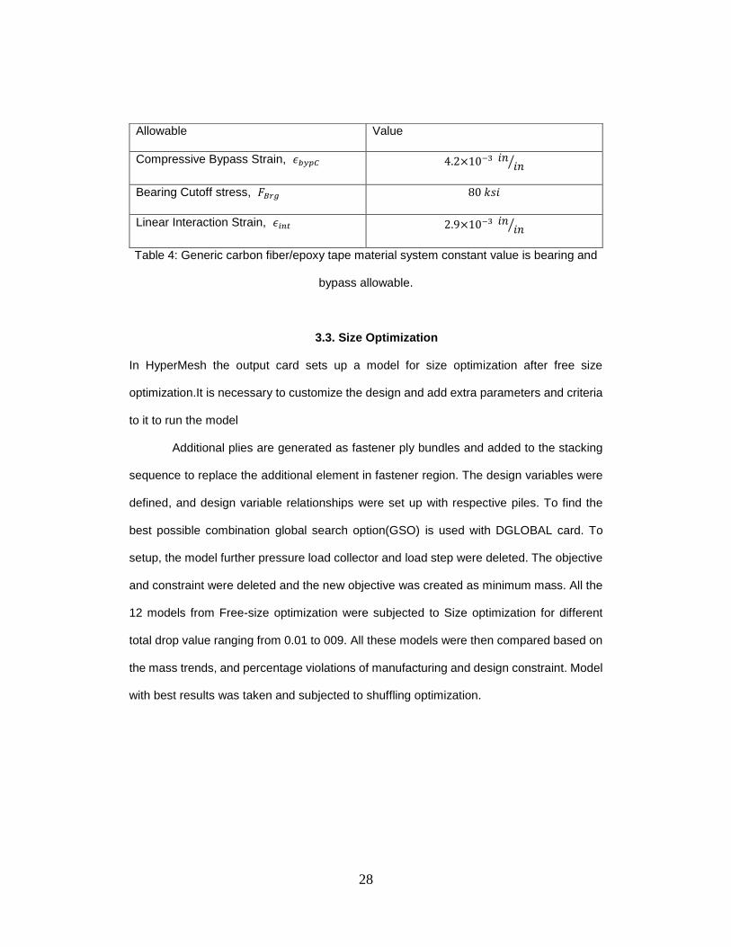
Bearing – Bypass Criteria

The bearing and bypass constraints were enforced at fastener locations. These

limitations were defined at two end points at fastener locations that captured peak loads

which cover fastener locations. The bearing stresses were calculated based on Deepak

Poliaki’s thesis study1.

𝜖𝑙𝑖𝑚 is shown as the upper allowable boundary and is the tensile constraint used in the

bearing land region in the optimization.

28

Table 4: Generic carbon fiber/epoxy tape material system constant value is bearing and

bypass allowable.

3.3. Size Optimization

In HyperMesh the output card sets up a model for size optimization after free size

optimization.It is necessary to customize the design and add extra parameters and criteria

to it to run the model

Additional plies are generated as fastener ply bundles and added to the stacking

sequence to replace the additional element in fastener region. The design variables were

defined, and design variable relationships were set up with respective piles. To find the

best possible combination global search option(GSO) is used with DGLOBAL card. To

setup, the model further pressure load collector and load step were deleted. The objective

and constraint were deleted and the new objective was created as minimum mass. All the

12 models from Free-size optimization were subjected to Size optimization for different

total drop value ranging from 0.01 to 009. All these models were then compared based on

the mass trends, and percentage violations of manufacturing and design constraint. Model

with best results was taken and subjected to shuffling optimization.

Allowable Value

Compressive Bypass Strain, 𝜖𝑏𝑦𝑝𝐶 4.2×10−3 𝑖𝑛 𝑖𝑛⁄

Bearing Cutoff stress, 𝐹𝐵𝑟𝑔 80 𝑘𝑠𝑖

Linear Interaction Strain, 𝜖𝑖𝑛𝑡 2.9×10−3 𝑖𝑛 𝑖𝑛⁄

29

3.4 Shuffling optimization on optimized composite laminate

The best model was selected from the previous study1 with pressure load 2, total

slope 0.05 and total drop 0.06. The output card sets up the model but just like the last step

we need to edit the model. All other design variables except DCOMP, which is to be a

design variable for shuffling step optimization, are to be deleted. All the design relationship

variables and design equation must be deleted as there is no need of any of those

equations. The objective is to minimize mass with the aim to find optimal stacking sequence

with Design variable DCOMP. Manufacturing constraints include limiting maximum

successive ply-drops up to 4, and the cover which is pre-defined stacking sequence which

remained unchanged. The cover constraint is needed after optimization to avoid possible

edge effects, and the comp is defined. The responses are the same as that of size

optimization, that is, mass, buckling, maximum strain, minimum strain, and CFailure. Out

of which buckling, maximum strain, minimum strain, and CFailure is constrained.

3.4.1 Buckling Criteria

The previous study1 developed Static structural stability by limiting lower limit on buckling

eigenvalue during sizing optimization. The procedure to generate ply shapes is more

resistant to buckling failure. In optimization process, the buckling eigenvalue is constrained

to be greater than 1.02 for the compression and shear load cases.

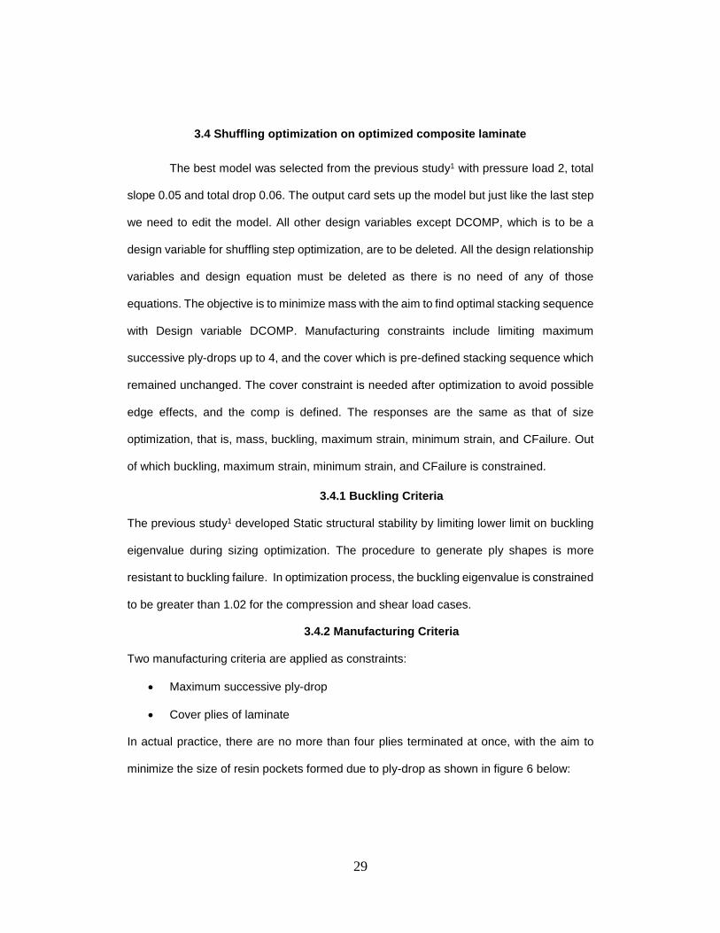
3.4.2 Manufacturing Criteria

Two manufacturing criteria are applied as constraints:

Maximum successive ply-drop

Cover plies of laminate

In actual practice, there are no more than four plies terminated at once, with the aim to

minimize the size of resin pockets formed due to ply-drop as shown in figure 6 below:

30

Figure 6: Ply-drop schematic

These resin pockets create material and geometric discontinuity due to which interlaminar

stress are introduced within the piles resulting into delamination. Hence, the number of

plies dropped are controlled to minimize the size of resin pocket.

Cover piles are stacked as [-45/90/45/0] to avoid a sudden change in orientation,

to maintain dimensional stability, and to prevent edge effect. As these kinds of layups are

symmetric and stable, hence, eliminates any local unbalanced induced forces.

3.4.3 Validation of stacking sequence

Stacking sequence was validated by checking whether it

satisfies the following rules4:

1. The layup should be balanced and symmetric.

2. At least 10% of all orientation should be present i.e. at least

10% of 0, 90, 45, -45.

3. No more than four plies of same orientation should be

stacked together

4. Place 0 and -/+45 as far as possible from the neutral axis.

5. Place -/+45 plies to cover laminate to avoid low-speed

impact.

6. Avoid external ply-drop. Ply-drop should be symmetric, and

the distance between successive ply-drop should be 10 -15

times of that of ply-drop.

Figure 7: Optimized stacking sequence

Symmetric layup – total 70 plies

COVER Plies

COVER Plies

31

3.4 Editing FEM model to CAD model

CAD GEOMETRY EDITING

After stacking sequence, it’s important to have ply shapes for manufacturing.

Figure below shows ply shapes after shuffling optimization; the spikes at the edges are

elements generated by mesh and would be tough to cut. Hence, ply smoothing process

was followed to obtain smooth contours for easing the ply cutting process and minimize

material loss.

Figure 8: unedited ply shapes

STEP 1: Ply smoothing and surface generation

There is a command in HyperMesh GUI to perform ply smoothing process and

generate lines and surfaces for the plies simultaneously.

User profile-> Engineering solutions ->Aerospace->composites->ply smoothing

32

Following parameters were used to generate smooth surface

The iteration was smoothing the ply shapes with splines and curves which were hard to

edit in further steps for creating a manufacture-able shape hence the number of iteration

was set to 0.

Step 2: EXPORT STEP FILE TO SOLIDWORKS

After ply smoothing process, surfaces were generated for each ply of the laminate.

Go to Export-> Geometry ->

Step 3: Edit plies surface in SolidWorks based on rules1 as shown below:

1. Holes or gaps along the fiber direction

If hole or gap is less than 100% of tow length requirement, then elements

are added to fill area

Fill holes, if drilling holes are possible in post manufacturing stage.

2. Tow dimensions along the fiber direction—0º and 90º plies

Must be greater than 2" (fiber direction) x 0.50" (transverse direction)

Figure 9: HyperMesh GUI command for ply smoothing and surface generation

33

If tow dimension is less than 50% of tow length/width requirement, then

elements within area are removed

If tow dimension is greater than 50% of tow length/width requirement, then

elements within area are added until minimum dimension requirement is

satisfied

3. Tow dimensions along the fiber direction—±45º plies

Must be greater than 2” x 2” to ensure balance constraint enforced

If tow dimension is less than 50% of tow length/width requirement, then elements

within area are removed

If tow dimension is greater than 50% of tow length/width requirement, then

elements within area are added until minimum dimension requirement is satisfied

and the gaps are filled

Figure 10: Edited ply shapes

Step 4: Converting to solids and making engineering drawing for full-scale print out.

SOLIDWORKS part drawing was generated and the paper size was set to real proportions.

34

For printout UTA racing plotter was used to take 20” x 10” print out as fixed in the print

command of SOLIDWORKS.

STEP 5: NESTING process

This process helped to estimate the amount of material required and saved the material

loss to make ply cutting efficient especially for which proved to be efficient

3.5 Manufacturing

The effective layup of such kind of complex laminate Traditional hand layup was done using

prepreg and laminate was cured in an autoclave. For manufacturing, the stacking

sequence was decided by results obtained by shuffling optimization results and the ply

shapes were taken from edited cad model after optimization process.

Material: Hexcel IM6/3506-1

Tooling: aluminum plate of 12” x 40” x 0.125” with vacuum valve

Cleaning agent: – Zyvax surface cleaner – Un1263

Sealant: Zyvax Sealer- Un1866

Release agent: Zyvax Multishield – Un1865

3.6.1 PLY CUTTING

The best way of cutting this type of ply shapes is to feed .dxf file to the ply cutting

machine, but due to lack of resources manual ply cutting was done. To cut different

irregular shapes paper templates were printed to true scale. As discussed in section 3.5.

Figure 11: Ply arrangement for cutting through nesting process

35

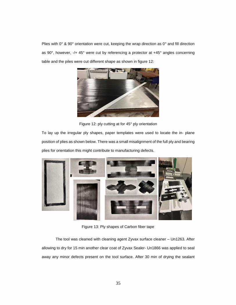
Plies with 0° & 90° orientation were cut, keeping the wrap direction as 0° and fill direction

as 90°, however, -/+ 45° were cut by referencing a protector at +45° angles concerning

table and the piles were cut different shape as shown in figure 12:

Figure 12: ply cutting at for 45° ply orientation

To lay up the irregular ply shapes, paper templates were used to locate the in- plane

position of plies as shown below. There was a small misalignment of the full ply and bearing

plies for orientation this might contribute to manufacturing defects.

3.6.2 Tool prep

The tool was cleaned with cleaning agent Zyvax surface cleaner – Un1263. After

allowing to dry for 15 min another clear coat of Zyvax Sealer- Un1866 was applied to seal

away any minor defects present on the tool surface. After 30 min of drying the sealant

Figure 13: Ply shapes of Carbon fiber tape

36

coating, a final coat of Release agent Zyvax Multishield – Un1865 was done on a tool for

Assuring a smooth release of parts.

3.6.3 LAYUP

For accurate layup, two corners were matched with the previously laid ply to

maintain fiber orientation consistently. This technique is timing consuming and requires lots

practice for high accuracy layup. A rectangular fixture would have contributed more

towards the precision of the layup.

Plies of 0 and 90 orientations were easy to a layup, -/+ 45 orientation plies, especially the

bearing plies were tight, and even a slight change in orientation would create an

unbalanced. As the laminate was thick, Debulking process was done after layup of every

ten plies to minimize possible amount voids.

3.6.4 VACCUM BAGGING

After layup was complete, a non-perforated release film was placed on the top of

laminate followed by breather or bleeder to allow escape excess of air and absorb excess

Figure 14: Lay-up process, release film, and breather

37

resin. The edges were covered with high-temperature tape to avoid any uneven flow

through edges as the laminate were thick.

Figure 15: Vacuum bagging

3.6.5 AUTOCLAVE CURE CYCLE

Curing process was done in an autoclave. The cycle was programmed as per datasheet of

Hexcel 3506-1 resin system as follows

1. Apply full vacuum and 85 psig pressure.

2. Heat at 3–5°F (1.8–3°C)/minute to 240°F (116°C).

3. Hold at 240°F (116°C) for 60–70 minutes.

4. Raise pressure to 100 psi; vent vacuum.

5. Raise temperature to 350°F (177°C) at 3–5°F (1.8–3°C)/minute.

6. Hold at 350°F (177°C) for 120 ± 10 minutes.

7. Cool at 2–5°F (1.2–3°C) to 100°F (38°C) and vent pressure.

38

3.6 Manufacturing Induced Defects

3.7 Manufacturing induced defects

Manufactured laminate is as shown in figure 13, warpage of with small magnitude was

observed in laminate at the transition of bearing plies to pad region and hence further study

was carried as described in chapter 4 to predict behavior and magnitude of warpage. It is

hard to measure the magnitude of warpage due to unavailability of resources, but the

behavior was recorded by observing the laminate.

The laminate was warped in upward along the transition region as marked in red in

figure X shown below

Figure 16: Demo cure cycle of HEXCEL IM6/3506-1.

Figure 17: Cured laminate with warpage

39

CHAPTER 4: Warpage Prediction Model

The focus of this section establishes a relationship between Fiber orientation, ply-

drops, and warpage effect due to this variation. The design of Experiments method was

followed to predict behavior and magnitude of warpage. An analytical model, FEM and

Experimental Model different number of ply drop for [0/45/90] family were developed to

compare results for thermal loading on the laminate during cooling process of cure cycle.

With the results of the analytical model for predicting warpage, it could be used to eliminate

the defect in optimization process of the composite laminate in the design phase.

4.1 Analytical Model for predicting Warpage due to cooling cycle in cure process

The analytical model focuses mainly on calculating out of plane deformation due

to thermal stress induced during cure cycle at the ply-drop intersection. The model can

also handle asymmetric and unbalanced layup on the side of ply-drop (Zone 1 & 2) as

shown figure 18(a) to give results regarding displacement in Z-direction.

Following FBD explains the effect of thermal forces and moment associated to it

Zone 1

Zone 2

Figure 18(a): Actual ply-drop intersection FBD

Figure 18(b): Modified ply-drop intersection FBD

Zone 1 h

1

h2

Hexp

d

ℎ1 2⁄ ℎ

2/2 ℎ

2/2

Nth1

Nth_resultant_L

Nth2

Nth_resin

ℎ2/2

Nth_resultant_U

Hexp

/2 Zone 2

40

Zone 1 is thick laminate, and zone 2 is thin laminate, the triangle in figure X(a) represents

the resin pocket with height Hd. Where Hd = tply *number of plies dropped & tply is post-

cured ply thickness of a single lamina. h1 & h2 height, Nth1 & Nth2 are the thermal forces

due to the CTE of laminate for zone 1 and zone 2 respectively.

Shown above is a schematic diagram of the procedure followed to explain the

analytical model to calculate displacement in X, Y & Z direction. As of now, we are plotting

displacement in Z-direction, but the same could be used to calculate X-Y displacement.

Material properties like Young’s modulus, Poison's ratio, modulus of rigidity, post-

cure ply thickness and the temperature difference in cure cycle in local direction as the

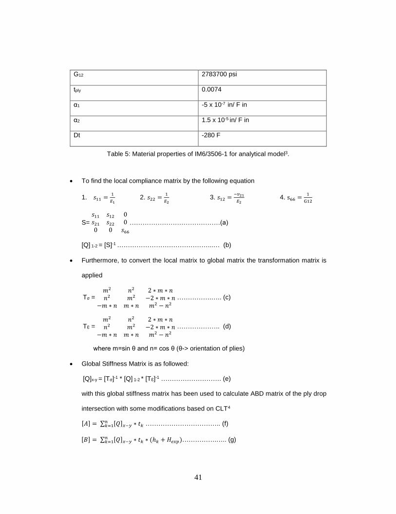
table shown below

Material properties Values

E1 22000000 psi

E2 1300000 psi

v12 0.3

Figure 19: schematic of analytical model

41

G12 2783700 psi

tply 0.0074

α1 -5 x 10-7 in/ F in

α2 1.5 x 10-5 in/ F in

Dt -280 F

To find the local compliance matrix by the following equation

1. 𝑠11 =1

𝐸1 2. 𝑠22 =

1

𝐸2 3. 𝑠12 =

−𝑣21

𝐸2 4. s66 =

1

G12

S=

𝑠11 𝑠12 0𝑠21 𝑠22 00 0 𝑠66

……………………………………(a)

[Q] 1-2 = [S]-1 ……………………………………...… (b)

Furthermore, to convert the local matrix to global matrix the transformation matrix is

applied

Tσ = 𝑚2 𝑛2 2 ∗ 𝑚 ∗ 𝑛𝑛2 𝑚2 −2 ∗ 𝑚 ∗ 𝑛

−𝑚 ∗ 𝑛 𝑚 ∗ 𝑛 𝑚2 − 𝑛2

…………….….. (c)

TƐ = 𝑚2 𝑛2 2 ∗ 𝑚 ∗ 𝑛𝑛2 𝑚2 −2 ∗ 𝑚 ∗ 𝑛

−𝑚 ∗ 𝑛 𝑚 ∗ 𝑛 𝑚2 − 𝑛2

……………….. (d)

where m=sin θ and n= cos θ (θ-> orientation of plies)

Global Stiffness Matrix is as followed:

[Q]x-y = [Tσ]-1 * [Q] 1-2 * [TƐ]-1 ………………………. (e)

with this global stiffness matrix has been used to calculate ABD matrix of the ply drop

intersection with some modifications based on CLT4

[𝐴] = ∑ [𝑄]𝑥−𝑦 ∗ 𝑡𝑘𝑛𝑘=1 …………………………….. (f)

[𝐵] = ∑ [𝑄]𝑥−𝑦 ∗ 𝑡𝑘 ∗ (ℎ𝑘 + 𝐻𝑒𝑥𝑝)𝑛𝑘=1 …………….….. (g)

Table 5: Material properties of IM6/3506-1 for analytical model3.

42

[𝐷] = ∑ [𝑄]𝑥−𝑦(𝑡𝑘 ∗ (ℎ𝑘 + 𝐻𝑒𝑥𝑝)2

+𝑡𝑘

3

12)𝑛

𝑘=1 …….…… (h)

Where Hexp = ℎ𝑑

6+

ℎ2

2 & tk is the ply thickness of kth layer & hk is the height kth layer

from bottom.

Thermal forces and moments calculated4 as

𝑁𝑡ℎ = ∑{[𝑄]𝑥−𝑦 ∗ [𝛼]𝑥−𝑦 ∗ (ℎ𝑘+1 − ℎ𝑘)} ∗ 𝛥𝑇

𝑛

𝑘=1

𝑀𝑡ℎ = ∑ {[𝑄]𝑥−𝑦 ∗ [𝛼]𝑥−𝑦 ∗ (ℎ𝑘+12 − ℎ𝑘

2)} ∗ (𝛥𝑇

2)𝑛

𝑘=1

ply-drop intersection has the plies on the upper and lower part of resin pocket.

Hence, the thermal load gets induced due to the both zone 1 and zone 2 as shown in

FBD and is assumed to be as

Nth_resultant_U = Nth_resultant_L = Nth1-Nth2

2

But the overall force on the intersection of ply-drop is

Neq = Nth_resultant_U + Nth_resultant_L + Nth_resin

Moment generated due this unbalanced thermal force is

Meq = Nth_resultant_U * (Hexp+ℎ2

2⁄ +ℎ2

2⁄ ) + Nth_resultant_L * ℎ2

2⁄ + Nth_resin * (𝐻𝑒𝑥𝑝

2⁄ +

ℎ22⁄ )

(Nth_resin ~ 0)

The strain and curvatures are calculated as

[εk

]= [𝐴 𝐵𝐵 𝐷

]-1 [𝑁𝑒𝑞𝑀𝑒𝑞

]

By classical lamination plate theory deformations U, V and W in X,Y and Z direction

respectively is

U= ε ∗ x +1

2∗ ε ∗ y

43

V= ε ∗ y +1

2∗ ε ∗ x

W= - 1

2(k ∗ 𝑥2 + k ∗ 𝑥2 + k ∗ x ∗ y)

where x and y are the matrices by which geometric dimension could be defined in

the x-y plane. Please refer Appendix for MATLAB code.

4.2 Experimental model - Fabricating coupons

Experimental model is set of coupons with a different combination of orientation

and number of ply drop as in table X. The coupons predict the behavior of the post cured

laminate and if possible try to measure the flatness of the coupons to measure magnitude

to get actual experimental data to set a baseline of comparison with the analytical model

and FEM.

Coupons were made 1” X 4” with ply-drop of 1, 2, 3, 4, 8, 12, 16, 24 with stacking

sequence with 0, -/+ 45, 90 families with gradual ply-drops for some ply-drops from 1-6 and

sudden ply-drops from 1-20 as mentioned in the table below:

Orientation No. of Ply-drops

0 1 2 3 4 5 6 8 12 16

-/+ 45 1 2 3 4 5 6 8 12 16

90 1 2 3 4 5 6 8 12 16

Procedure for making coupons was same as mentioned in section 3.6 except the

3.6.3. Layup for each coupon is done as a set of all 0 for each coupon with two cover plies

at the top and two cover plies at the bottom. The similar layup was followed for 90, but in

the case of -/+45, a balance was to be maintained to avoid any unbalanced forces as the

aim was to record. The deformation due to ply drops for each -45 angled ply there was 45

Table 6: Experimental model for different combination ply-drop and orientation

44

angled ply for some ply drops with the top and bottom cover comprising a pair of -/+45

plies.

For example, stacking sequence for 4 ply drop layup for 0 and 90 was done as

[0 0 0 0 0 0 0 0] and [90 90 90 90 90 90 90 90] respectively but for -/+ 45 it was

[-45 45 -45 45 45 -45 45- 45]. This was done to layup a balanced and symmetric

laminate.

Curing of all coupons was done all in a single cure and only tool with same procedure just

one time to avoid any variation due to obvious errors of autoclave process. Hence the

results were easily comparable.

Figure 20 (b): Coupons after cure

Figure 20 (a): Coupons before cure

45

After curing it was observed that the factors causing warpage were majorly due to free

expansion. Hence, another set of coupons were made with new layup technique to

replicate the real senior as that in the composite laminate by restricting edges. To pick up

the warpage caused due to the moment generated by ply-drop as explained in section

4.1. Therefore to restrict the edges for avoiding warpage effect due to free expansion,

setup, as shown in the figure, was followed.

4.3 FEM model for predicting Warpage due to cooling cycle in cure process

Varying mesh size throughout overall coupon creates with 3D elements to pick up

the displacement due to the ply-drop intersection in Z-direction (out-place displacement).

Following is the setup of FEM model to predict the out of plane warpage.

Orientation No. of Ply-drops

0 16 20 24

-/+ 45 16 20 24

90 16 20 24

Figure 21: Coupons with restricted edges. Table 7: Experimental model for

different combination ply-drop and orientation with restricted edges

46

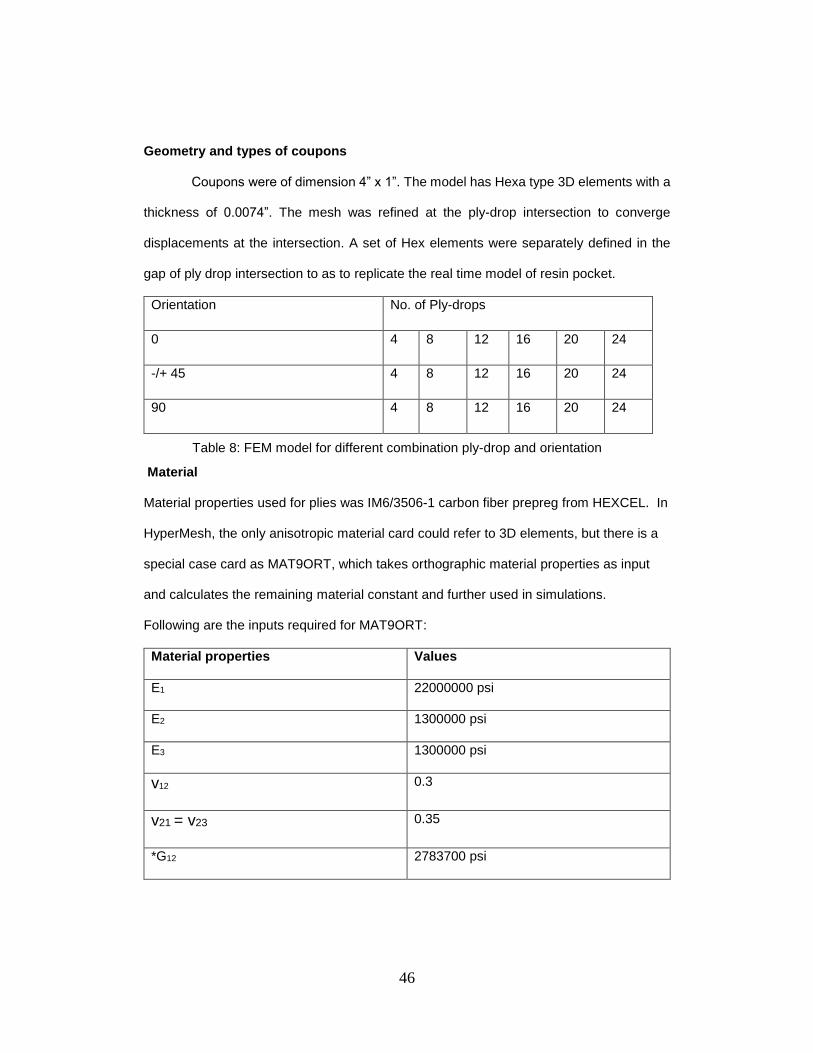
Geometry and types of coupons

Coupons were of dimension 4” x 1”. The model has Hexa type 3D elements with a

thickness of 0.0074”. The mesh was refined at the ply-drop intersection to converge

displacements at the intersection. A set of Hex elements were separately defined in the

gap of ply drop intersection to as to replicate the real time model of resin pocket.

Orientation No. of Ply-drops

0 4 8 12 16 20 24

-/+ 45 4 8 12 16 20 24

90 4 8 12 16 20 24

Material

Material properties used for plies was IM6/3506-1 carbon fiber prepreg from HEXCEL. In

HyperMesh, the only anisotropic material card could refer to 3D elements, but there is a

special case card as MAT9ORT, which takes orthographic material properties as input

and calculates the remaining material constant and further used in simulations.

Following are the inputs required for MAT9ORT:

Material properties Values

E1 22000000 psi

E2 1300000 psi

E3 1300000 psi

v12 0.3

v21 = v23 0.35

*G12 2783700 psi

Table 8: FEM model for different combination ply-drop and orientation

47

*G23 321090 psi

*G31 2997900 psi

α1 -5 x 10-7 in/ F in

α2 1.5 x 10-5 in/ F in

Tref (the material temperature) 350 F

* Manually calculated values refer Appendix for MATLAB program and explanation

Table 9: Material properties for IM6/3506-1 prepreg

For the assigning material properties to the resin, MAT1 was used as it takes isotropic

material properties as mentioned in the following table:

Material properties Values

E 1300000 psi

V 0.35

G 750000 psi

Α 1.5 x 10-5 in/ F in

Tref (the material temperature) 350 F

Table 10: Material properties for 3506-1

Property

In HyperMesh the type of elements is assigned its physical parameters like type of

element, coordinate system, material, etc., all through properties. In this model, PSOLID

property is used for both plies and resin.

Loads

Thermal load with a temperature gradient of -280 F was created to replicate the

cooling process of cure cycle. This load was created on to every node of the coupon. The

temperature distribution was assumed to be even, and the analysis was considered as a

time-independent form of simulation.

48

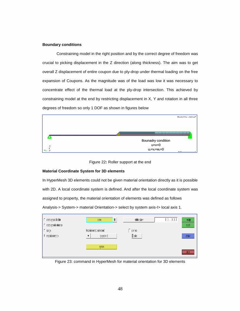
Boundary conditions

Constraining model in the right position and by the correct degree of freedom was

crucial to picking displacement in the Z direction (along thickness). The aim was to get

overall Z displacement of entire coupon due to ply-drop under thermal loading on the free

expansion of Coupons. As the magnitude was of the load was low it was necessary to

concentrate effect of the thermal load at the ply-drop intersection. This achieved by

constraining model at the end by restricting displacement in X, Y and rotation in all three

degrees of freedom so only 1 DOF as shown in figures below

Figure 22: Roller support at the end

Material Coordinate System for 3D elements

In HyperMesh 3D elements could not be given material orientation directly as it is possible

with 2D. A local coordinate system is defined. And after the local coordinate system was

assigned to property, the material orientation of elements was defined as follows

Analysis-> System-> material Orientation-> select by system axis-I> local axis 1.

Figure 23: command in HyperMesh for material orientation for 3D elements

Bounadry condition

u=v=0

ur=vr=wr=0

49

The model formation for the composite laminate for predicting warpage is same with same

loading conditions and similar boundary condition of roller support. The only change is the

geometry which is same as mentioned in 3.2.1. The property is the same PSOLID as used

for coupons only different property is defined for various orientation as for each orientation

a separate local axis has to be defined which can be only assigned to elements through

the property.

Chapter 5: Results

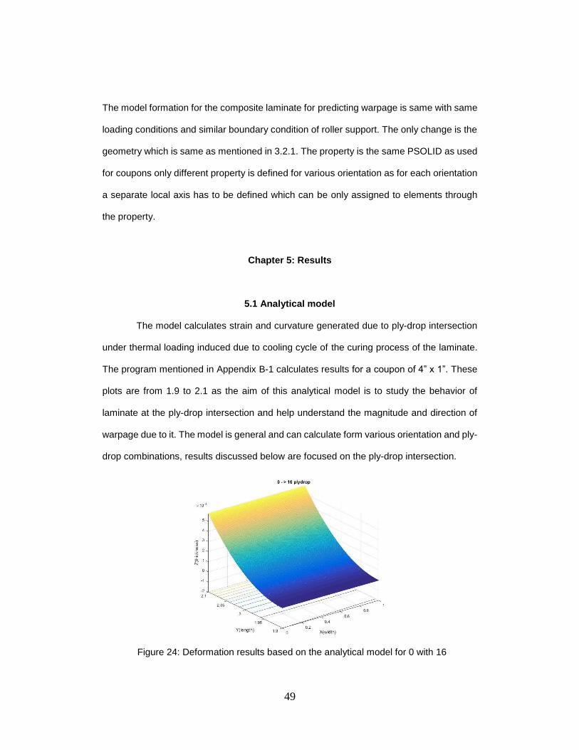
5.1 Analytical model

The model calculates strain and curvature generated due to ply-drop intersection

under thermal loading induced due to cooling cycle of the curing process of the laminate.

The program mentioned in Appendix B-1 calculates results for a coupon of 4” x 1”. These

plots are from 1.9 to 2.1 as the aim of this analytical model is to study the behavior of

laminate at the ply-drop intersection and help understand the magnitude and direction of

warpage due to it. The model is general and can calculate form various orientation and ply-

drop combinations, results discussed below are focused on the ply-drop intersection.

Figure 24: Deformation results based on the analytical model for 0 with 16

ply-drops

50

Figure 25: Deformation results based on the analytical model for 90 with 16 ply-drops

Figure 26: Deformation results based on the analytical model for -/+45 with 16 ply-drops

The above plot in figure 19, figure 20, and figure 21 is for 0, -/+45, and 90 orientations

respectively. The plot is X vs. Y vs. Z representing width, length, and thickness of coupons.

Out of plane deformation in positive Z-direction with 16 ply-drops from 2 to 2.1 on the y-

51

axis in figure 21. The small magnitude of warpage incrementing with length from the ply-

drop junction was observed and the direction was in positive Z-direction. In case, of -/+ 45

apart from the warpage along the length there was also twisting observed in the direction

of fiber orientation.

Results were obtained several model, and the angle of warpage was calculated as shown

below:

5.2 Experimental model

The experimental design comprised of a number of different combinations of

layups as mentioned in section 4.2. Out of which up to 16 ply-drop in all three combinations

of orientation. Due to unavailability of resources the magnitude of this warpage was not

4 8 12 16 20 24

0 0.2215 1.2147 2.3135 4.8146 5.4831 6.8747

45 0.3235 0.2279 0.2342 0.3413 0.3244 0.6402

90 0.2368 0.3204 0.4783 0.3661 0.5128 0.8302

0

1

2

3

4

5

6

7

8

θ°

No of ply-drops

Angle of Warpage for Analytical Model0 45 90

Figure 27: Trends of change in angle of with ply-drops and the orientation for Analytical model

θ°

Ply-drop intersection

52

possible as the warpage was in order ranging from 10-3 to10-4 of an inch and below. There

was visually noticeable warpage detected for -/+ 45 orientation the similar behavior as

predicted by the analytical model was observed. Hence more coupons with higher ply-

drops are needed to be fabricated for all three-different orientation. Going beyond 16 ply-

drop at a time would violate the actual design scenario. Below are the images of coupons

manufactured with 16 ply-drop in figure X and figure X has images for the coupons

fabricated below 16 ply-drop.

Figure 28: 0 orientation Layup with 16 ply-drop

Figure 29: -/+45 orientation Layup with 16 ply-drop

Figure 30: 90 orientation Layup with 16 ply-drop

53

With the new set of coupons with restricted edges showed similar result as that of the

coupons layed earlier. There was no measureable amount of warpage that could be

observed. But there was a deformation in -/+ 45° as due to the coupling effect due to the

presence of D16 and D26 which collectively causes bending twisting effect, coupling effect.

Figure 32(a): Coupons with restricted edges after cure

Figure 31: coupling effect for a classical lamination theory34

54

The possible reasons for not obtaining warpage could be:

The pressure during cure cycle acts on vacuum bag which restricts the z-direction

warpage. Out of plane deformation occurs due to the moment generated at plydrop

intersection, the values could be obtatined from analytical model as 25.3964 lbf-in for 0°,

6.7743 lbf-in for 90° and 9.5768 lbf-in for -/+ 45° which is less than counter moment

generated at ply-drop intersection due to vacuum bag exerting pressure of 100 psi over

the area of 2” x 1” on thin laminate. Assuming a point load of magintute 50 lbf at midpoint

of the area. This force creates a counter moment of 50 lbf-in. Hence, overriding the effect

of moment generated by thermal force as shown in figure below:

There is need of a layup technique by which the warpage due ply-drop effect could be

amplified enough to measure and calibrate the analytical model in order to yield accurate

results.

5.3 FEM model

Fem could predict the effect of ply-drop on the entire coupon. But the results were more

focused on the behavior of the ply-drop intersection.

Meq = 25.3964 lbf-in

Mv = 50 lbf-in

Fv =P/A = 100 psi/2 in2 = 50 lbs

1”

Figure 32 (b): Moment at ply-drop intersection

55

Figure 33(a): 0° plies with 16 ply-drops

Figure 33(b): 0° plies with 16 ply-drops 100x exaggerated

Warpage could be observed in figure 33(a) and Figure 33(b) after results are

exaggerated by 100x. Unequal displacement of the edges in Z-direction is possibly

because of the laminate thickness difference. The thin laminate over left of ply-drop

intersection is displaced more cause of less weight to resist compared to the thick laminate

at right.

56

Figure 34(a): 90° plies with 16 ply-drops

Figure 34(b): 90° plies with 16 ply-drops 100x exaggerated

Figure 34(a) and figure 34(b) results plots for 90° ply orientations and the magnitude is

higher compared to 0 ply orientation, but the behavior is similar, that is there is an

incremental change in length away from the ply-drop intersection in both direction.

57

Figure 35(a): -/+45° plies with 16 ply-drops

Figure 35(b): -/+45° plies with 16 ply-drops 100x exaggerated

The results are shown in figure 35(a) and Figure 35(b) is for -/+45° ply orientation. It is

observed that warpage is a function of length and width and due to which twisting is the

effect is induced.

Below is the trend which shows the change in angle at ply-drop intersection

58

angle of warpage increases the number of ply-drop increases.

Angle of warpage is quite low in magnitude. Sudden change in 0° compared to 90° and -

/+ 45° can be observed, reason for this is fiber in line transfers moment generated with less

matrix resistance compared to 90° and -/+ 45°.

4 8 12 16 20 24

0 0.0049 1.0405 2.1598 4.6509 5.2904 6.6669

45 0.1183 0.0727 0.0673 0.1343 0.1052 0.4073

90 0.0208 0.1284 0.2079 0.2864 0.3085 0.3366

012345678

θ°

No of ply-drops

ANGLE OF WARPAGE for FEM

0 45 90

Figure 36: Trends of change in angle of with ply-drops and the orientation for FEM

59

5.4 Comparison of results from all three models

For validation of analytical model and FEM, the results are compared as follows

This results are in close agreement, but in general the models are not reliable until the

analytical model is calibrated with the responses from experimental model.

FEM with 3D elements generated of fabricated composite laminate.

4 8 12 16 20 24

0-fem 0.0049 1.0405 2.1598 4.6509 5.2904 6.6669

45-fem 0.1183 0.0727 0.0673 0.1343 0.1052 0.4073

90-fem 0.0208 0.1284 0.2079 0.2864 0.3085 0.3366

0-A 0.2215 1.2147 2.3135 4.8146 5.4831 6.8747

45-A 0.3235 0.2279 0.2342 0.3413 0.3244 0.6402

90-A 0.2368 0.3204 0.4783 0.3661 0.5128 0.8302

0

1

2

3

4

5

6

7

8

θ°

No of ply-drops

0-fem 45-fem 90-fem 0-A 45-A 90-A

Figure 37: Comparison of FEM and Analytical results

60

Figure 38: Z-displacement for composite laminate after thermal loading

It was observed than the maximum Z-displacement could be seen in the same location

as that of in the actual laminate as shown in figure 17.

Chapter 6: Conclusion & Future work:

In three phase optimization process, several models were subjected to optimization

process with a combination of different values of total ply slope and total ply drop in free-

size and size optimization in the previous study1.

…………..(a)

…………..(b)

Figure 39: (a) Ply drop and slope effect on larger panel1 (b) Ply drop effect on

smaller panel1

The value of total ply slope and total ply drop assigned in three-phase optimization process

should have a minimum range of variation. To get manufacture-able stacking sequence

𝛥𝑠

𝛥𝑠

61

with minimum constraint violation. By manufacturing the complete laminate with variable

ply-drops series of ply drops as shown in figure

The warpage due ply-drops could be induced in thick laminates due to manufacturing

process because of the set of the moment generated by each ply-drop in the entire

laminate.

Results from the Analytical model and FEM are in close agreement in warpage prediction

due to ply-drops during the manufacturing process. The analytical model is computationally

fast and suitable for integration into the automated optimization process to eliminate

defects in the design phase after further refinment of model based on the responses from

DOE.

FUTURE WORK 1. Layup of coupons has to be done to increase the moment generated at ply-drop

intersection which will be more than the counter moment generated due to vacuum

bagging and cure cycle pressure to get a measurable warpage with different

combination of ply-drops and stacking sequence.

Following are some suggestion for the same:

i. Increase the cover plies from four to eight

ii. Change the material which requires low pressure for cure.

2. After the measurable warpage, could be mapped from experimental model the height

of resin pocket Hexp mentioned in FBD figure 18(b) has to be calibrate to refine the

analytical model.

3. Transient analysis could be performed, stiffness matrix and thermal load could be

made time dependent.

Figure 40: Cross-sectional view of optimize composite plate

62

4. Exact Temperature distribution can be found from thermal analysis and accordingly

thermal load could be applied, or a combined structural and thermal analysis could

be done to refine FEM and compare results with experimental model to validate

results.

5. Detection of resin pockets through nondestructive testing and Analysis for prediction

of knock down strength could be carried out.

APPENDIX A

FEM file structure for shuffling optimization

$$ $$ Optistruct Input Deck Generated by HyperMesh Version : 14.0.130.21 $$ Generated using HyperMesh-Optistruct Template Version : 14.0.130 $$ $$ Template: optistruct $$ $$ $$ optistruct $ RESPRINT=EQUA OUTPUT,SZTOSH,YES SCREEN OUT CFAILURE(H3D,NDIV=1) = ALL CSTRAIN(H3D,ALL,NDIV=1) = YES CSTRESS(H3D,ALL,NDIV=1) = ALL $$------------------------------------------------------------------------------$ $$ Case Control Cards $ $$------------------------------------------------------------------------------$ $$ $$ OBJECTIVES Data $$ $ $HMNAME OBJECTIVES 1objective $ DESOBJ(MIN)=15 $ $ $HMNAME LOADSTEP 1"Shear_Only" 1 $ SUBCASE 1 LABEL Shear_Only SPC = 8 LOAD = 2 DESSUB = 15 $ $HMNAME LOADSTEP 2"buck_Shear_Only" 4 $

63

SUBCASE 2 LABEL buck_Shear_Only SPC = 8 METHOD(STRUCTURE) = 1 STATSUB(BUCKLING) = 1 DESSUB = 16 $ DESSUB = 17 $ $HMNAME LOADSTEP 3"Compression_Only" 1 $ SUBCASE 3 LABEL Compression_Only SPC = 8 LOAD = 3 DESSUB = 17 $ $HMNAME LOADSTEP 4"buck_Compression_Only" 4 $ SUBCASE 4 LABEL buck_Compression_Only SPC = 8 METHOD(STRUCTURE) = 1 STATSUB(BUCKLING) = 3 DESSUB = 18 $ DESSUB = 19 $ $HMNAME LOADSTEP 5"Tension" 1 $ SUBCASE 5 LABEL Tension SPC = 8 LOAD = 4 DESSUB = 19 $$-------------------------------------------------------------- $$ HYPERMESH TAGS $$-------------------------------------------------------------- $$BEGIN TAGS $$END TAGS $ BEGIN BULK $ $HMNAME PLYS 1"PLYS_1" $HWCOLOR PLYS 1 4 PLY 1 2 0.005 -45.0 YES 0.005 + 7 $ $HMNAME PLYS 2"PLYS_2" $HWCOLOR PLYS 2 3 PLY 2 2 0.005 0.0 YES 0.005 + 2

64

$ $HMNAME PLYS 3"PLYS_3" $HWCOLOR PLYS 3 5 PLY 3 2 0.005 45.0 YES 0.005 + 11 $ $HMNAME PLYS 4"PLYS_4" $HWCOLOR PLYS 4 6 PLY 4 2 0.005 90.0 YES 0.005 + 16 $ $HMNAME PLYS 5"PLYS_5" $HWCOLOR PLYS 5 4 PLY 5 2 0.005 -45.0 YES 0.005 + 21 $ $HMNAME PLYS 6"PLYS_6" $HWCOLOR PLYS 6 4 PLY 6 2 0.005 -45.0 YES 0.005 + 36 $ $HMNAME PLYS 7"PLYS_7" $HWCOLOR PLYS 7 4 PLY 7 2 0.005 -45.0 YES 0.005 + 37 $ $HMNAME PLYS 8"PLYS_8" $HWCOLOR PLYS 8 5 PLY 8 2 0.005 45.0 YES 0.005 + 38 $ $HMNAME PLYS 9"PLYS_9" $HWCOLOR PLYS 9 4 PLY 9 2 0.005 -45.0 YES 0.005 + 38 $ $HMNAME PLYS 10"PLYS_10" $HWCOLOR PLYS 10 5 PLY 10 2 0.005 45.0 YES 0.005 + 38 $ $HMNAME PLYS 11"PLYS_11" $HWCOLOR PLYS 11 5 PLY 11 2 0.005 45.0 YES 0.005 + 22 $ $HMNAME PLYS 12"PLYS_12" $HWCOLOR PLYS 12 24 PLY 12 2 0.005 45.0 YES 0.005 + 36

65

$ $HMNAME PLYS 13"PLYS_13" $HWCOLOR PLYS 13 5 PLY 13 2 0.005 45.0 YES 0.005 + 37 $ $HMNAME PLYS 14"PLYS_14" $HWCOLOR PLYS 14 3 PLY 14 2 0.005 0.0 YES 0.005 + 2 $ $HMNAME PLYS 15"PLYS_15" $HWCOLOR PLYS 15 3 PLY 15 2 0.005 0.0 YES 0.005 + 2 $ $HMNAME PLYS 16"PLYS_16" $HWCOLOR PLYS 16 3 PLY 16 2 0.005 0.0 YES 0.005 + 4 $ $HMNAME PLYS 17"PLYS_17" $HWCOLOR PLYS 17 3 PLY 17 2 0.005 0.0 YES 0.005 + 5 $ $HMNAME PLYS 18"PLYS_18" $HWCOLOR PLYS 18 6 PLY 18 2 0.005 90.0 YES 0.005 + 16 $ $HMNAME PLYS 19"PLYS_19" $HWCOLOR PLYS 19 3 PLY 19 2 0.005 0.0 YES 0.005 + 6 $ $HMNAME PLYS 20"PLYS_20" $HWCOLOR PLYS 20 5 PLY 20 2 0.005 45.0 YES 0.005 + 12 $ $HMNAME PLYS 21"PLYS_21" $HWCOLOR PLYS 21 4 PLY 21 2 0.005 -45.0 YES 0.005 + 8 $ $HMNAME PLYS 22"PLYS_22" $HWCOLOR PLYS 22 5 PLY 22 2 0.005 45.0 YES 0.005 + 11

66

$ $HMNAME PLYS 23"PLYS_23" $HWCOLOR PLYS 23 5 PLY 23 2 0.005 45.0 YES 0.005 + 11 $ $HMNAME PLYS 24"PLYS_24" $HWCOLOR PLYS 24 4 PLY 24 2 0.005 -45.0 YES 0.005 + 7 $ $HMNAME PLYS 25"PLYS_25" $HWCOLOR PLYS 25 4 PLY 25 2 0.005 -45.0 YES 0.005 + 7 $ $HMNAME PLYS 26"PLYS_26" $HWCOLOR PLYS 26 5 PLY 26 2 0.005 45.0 YES 0.005 + 15 $ $HMNAME PLYS 27"PLYS_27" $HWCOLOR PLYS 27 4 PLY 27 2 0.005 -45.0 YES 0.005 + 10 $ $HMNAME PLYS 28"PLYS_28" $HWCOLOR PLYS 28 6 PLY 28 2 0.005 90.0 YES 0.005 + 19 $ $HMNAME PLYS 29"PLYS_29" $HWCOLOR PLYS 29 6 PLY 29 2 0.005 90.0 YES 0.005 + 38 $ $HMNAME PLYS 30"PLYS_30" $HWCOLOR PLYS 30 3 PLY 30 2 0.005 0.0 YES 0.005 + 38 $ $HMNAME PLYS 31"PLYS_31" $HWCOLOR PLYS 31 3 PLY 31 2 0.005 0.0 YES 0.005 + 37 $ $HMNAME PLYS 32"PLYS_32" $HWCOLOR PLYS 32 3 PLY 32 2 0.005 0.0 YES 0.005 + 36

67

$ $HMNAME PLYS 33"PLYS_33" $HWCOLOR PLYS 33 4 PLY 33 2 0.005 -45.0 YES 0.005 + 38 $ $HMNAME PLYS 34"PLYS_34" $HWCOLOR PLYS 34 3 PLY 34 2 0.005 0.0 YES 0.005 + 20 $ $HMNAME PLYS 35"PLYS_35" $HWCOLOR PLYS 35 3 PLY 35 2 0.005 0.0 YES 0.005 + 38 $$ $$ Stacking Information for Ply-Based Composite Definition $$ $ $HMNAME LAMINATES 3"LAM_3" $HWCOLOR LAMINATES 3 3 STACK 3 SYM 4 1 7 10 21 24 + 27 33 31 34 22 25 28 2 + 3 12 15 11 16 14 13 9 + 8 6 5 18 17 19 35 29 $ $HMNAME OPTICONTROLS 1"optistruct_opticontrol" 1 $ DOPTPRM DESMAX 1000 GBUCK 0 $ $HMNAME OPTITABLEENTRS 1"optistruct_tableentries" 14 $ DTABLE F1xt 0.0 F1yt 0.0 F2xt 2000.0 F2yt 0.0 + F1xc 0.0 F1yc 0.0 F2xc -2000.0 F2yc 0.0 + F1xs 2000.0 F1ys 0.0 F2xs 0.0 F2ys 2000.0 + Sym 2.0 diam 0.25 strnCmp 0.0042 BrgLim 80000.0 $HMNAME DESVARS 3DCOMP3.1 DSHUFFLE 3 STACK 3 + MAXSUCC ALL 4 + COVER 1 -45.0 0.0 45.0 90.0 $HMNAME DESVARS 3DCOMP3.1.1 DSHUFFLE 3 STACK 3 + MAXSUCC ALL 4 + COVER 1 -45.0 0.0 45.0 90.0 $$ $$ OPTIRESPONSES Data $$ DRESP1 15 Mass MASS DRESP1 69 BucklingLAMA 1

68

DRESP1 78 MaxStrn CSTRAIN PCOMP SMAP ALL 3 $$ $$ OPTICONSTRAINTS Data $$ $ $HMNAME OPTICONSTRAINTS 9MaxStrn $ DCONSTR 9 78-0.003 0.003 $ $HMNAME OPTICONSTRAINTS 10MinStrn $ DCONSTR 10 79-0.003 0.003 $ $HMNAME OPTICONSTRAINTS 11CFailure $ DCONSTR 11 80 1.0 $ $HMNAME OPTICONSTRAINTS 14BUCKLING $ DCONSTR 14 691.02 DCONADD 15 9 10 11 DCONADD 16 14 DCONADD 17 9 10 11 DCONADD 18 14 DCONADD 19 9 10 11 $HMNAME SYSTCOL 1 "auto1" $HWCOLOR SYSTCOL 1 3 $$ $$ SYSTEM Data $$ CORD3R 1 3101 7134 6011 $ $HMMOVE 2 $ 1THRU 8500 $$ $$------------------------------------------------------------------------------$ $$ HyperMesh name and color information for generic components $ $$------------------------------------------------------------------------------$ $HMNAME COMP 2"Middle Surface" 3 "CarbonTape" 4 $HWCOLOR COMP 2 52 $ $HMNAME COMP 3"component1" $HWCOLOR COMP 3 4

69

$ $HMNAME COMP 4"component2" $HWCOLOR COMP 4 5 $ $HMNAME COMP 5"component3" $HWCOLOR COMP 5 6 $ $ $ $HMNAME PROP 3"CarbonTape" 4 $HWCOLOR PROP 3 7 PCOMPP 3 BOTTOM 18000.0 STRN $$ $$ MAT8 Data $$ $HMNAME MAT 2"CarbonEpoxy" "MAT8" $HWCOLOR MAT 2 7 MAT8 22.2+7 1300000.0.3 750000.0 516000.00.056 + 0.5 0.4 70.0 170000.0170000.06500.0 28000.0 10000.0 $$ $$------------------------------------------------------------------------------$ $$ HyperMesh Commands for loadcollectors name and color information $ $$------------------------------------------------------------------------------$ $HMNAME LOADCOL 5"Compression" $HWCOLOR LOADCOL 5 5 $$ $HMNAME LOADCOL 6"Tension" $HWCOLOR LOADCOL 6 5 $$ $HMNAME LOADCOL 7"Shear" $HWCOLOR LOADCOL 7 5 $$ $HMNAME LOADCOL 8"Constraints" $HWCOLOR LOADCOL 8 5 $$ $$ EIGRL cards $$ $HMNAME LOADCOL 1"EIGRL" $HWCOLOR LOADCOL 1 7 EIGRL 1 0.0 2 MAX ENDDATA $$ $$------------------------------------------------------------------------------$$ $$ Data Definition for AutoDV $$ $$------------------------------------------------------------------------------$$ $$ $$-----------------------------------------------------------------------------$$ $$ Design Variables Card for Control Perturbations $$

70

$$-----------------------------------------------------------------------------$$ $$ $$------------------------------------------------------------------------------$ $$ Domain Element Definitions $ $$------------------------------------------------------------------------------$ $$ $$------------------------------------------------------------------------------$$ $$ Control Perturbation $$ $$------------------------------------------------------------------------------$$

APPENDEX B MATLAB code

B-1 Anylitical model %% By Sitanshu Pandya clear all; close all %% Material properties E1=22000000; E2=1300000; G12=2783700; v12=0.3; Alpha_12=[-5e-7;1.5e-5;0]; dT=280; %F tply=0.0074; %% S matrix S11=1/E1; S12=-v12/E1; S22=1/E2; S66=1/G12; S=[S11 S12 0; S12 S22 0; 0 0 S66]; %% Q matrix Q=inv(S); %% Stacking Sequence for ZONES % zone1=[90 90 90 90 90 90 90 90 90 90 90 90 90 90 90 90 90 90

90 90]; % zone2=[90 90 90 90]; zone1=[0 0 0 0 0 0 0 0 0 0 0 0 0 0 0 0 0 0 0 0]; zone2=[0 0 0 0]; % zone1=[-45 45 -45 45 -45 45 -45 45 -45 45 -45 45 45 -45 45 -45

45 -45 45 -45]; % zone2=[-45 45 45 -45];

%%%%%%%%%%%%%%%MATERIAL PROPERTIES FOR

RESIN%%%%%%%%%%%%%%%%%%%%%%%%%%%%%%%%%%%%%%%%%%%%%%%% E=18854.9059054; v=0.35; G=10877.83033; Alpha=1.5e-5; %NO> OF PLY DROPED no_of_ply_drop=16;

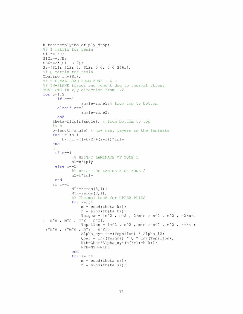
71

h_resin=tply*no_of_ply_drop; %% S matrix for resin S11r=1/E; S12r=-v/E; S66r=2*(S11-S12); Sr=[S11r S12r 0; S12r 0 0; 0 0 S66r]; %% Q matrix for resin Qbariso=inv(Sr); %% THERMAL LOAD FROM ZONE 1 & 2 %% IN-PLANE forces and moment due to thermal stress %CAL CTE in x,y direction from 1,2 for c=1:2 if c==1 angle=zone1;% from top to bottom elseif c==2 angle=zone2; end theta=fliplr(angle); % from bottom to top %% h b=length(angle) % how many layers in the laminate for i=1:b+1 h(:,i)=((-b/2)+(i-1))*tply; end h if c==1 %% HEIGHT LAMINATE OF ZONE 1 h1=b*tply else c==2 %% HEIGHT OF LAMINATE OF ZONE 2 h2=b*tply end if c==1 NTH=zeros(3,1); MTH=zeros(3,1); %% Thermal Load for UPPER PLIES for k=1:b m = cosd(theta(k)); n = sind(theta(k)); Tsigma = [m^2 , n^2 , 2*m*n ; n^2 , m^2 , -2*m*n

; -m*n , m*n , m^2 - n^2]; Tepsilon = [m^2 , n^2 , m*n ; n^2 , m^2 , -m*n ;

-2*m*n , 2*m*n , m^2 - n^2]; Alpha_xy= inv(Tepsilon) * Alpha_12; Qbar = inv(Tsigma) * Q * inv(Tepsilon); Nth=Qbar*Alpha_xy*(h(k+1)-h(k)); NTH=NTH+Nth; end for s=1:b m = cosd(theta(s)); n = sind(theta(s));

72

Tsigma = [m^2 , n^2 , 2*m*n ; n^2 , m^2 , -2*m*n

; -m*n , m*n , m^2 - n^2]; Tepsilon = [m^2 , n^2 , m*n ; n^2 , m^2 , -m*n ;

-2*m*n , 2*m*n , m^2 - n^2]; Alpha_xy= inv(Tepsilon) * Alpha_12; Qbar = inv(Tsigma) * Q * Tepsilon; Mth=Qbar*Alpha_xy*(h(s+1)^2-h(s)^2); MTH=MTH+Mth; end elseif c==2 NTH=zeros(3,1); MTH=zeros(3,1); %% Thermal Load for ZONE 2 for k=1:b m = cosd(theta(k)); n = sind(theta(k)); Tsigma = [m^2 , n^2 , 2*m*n ; n^2 , m^2 , -2*m*n

; -m*n , m*n , m^2 - n^2]; Tepsilon = [m^2 , n^2 , m*n ; n^2 , m^2 , -m*n ;

-2*m*n , 2*m*n , m^2 - n^2]; Alpha_xy= inv(Tepsilon) * Alpha_12; Qbar = inv(Tsigma) * Q * inv(Tepsilon); Nth=Qbar*Alpha_xy*(h(k+1)-h(k)); NTH=NTH+Nth; end

for s=1:b m = cosd(theta(s)); n = sind(theta(s)); Tsigma = [m^2 , n^2 , 2*m*n ; n^2 , m^2 , -2*m*n

; -m*n , m*n , m^2 - n^2]; Tepsilon = [m^2 , n^2 , m*n ; n^2 , m^2 , -m*n ;

-2*m*n , 2*m*n , m^2 - n^2]; Alpha_xy= inv(Tepsilon) * Alpha_12; Qbar = inv(Tsigma) * Q * Tepsilon; Mth=Qbar*Alpha_xy*(h(s+1)^2-h(s)^2); MTH=MTH+Mth; end end

if c==1 %% Thermal Load for zone 1 NTH1=NTH*dT %% Theraml Moments for zone 1 MTH1=MTH*(dT/2) elseif c==2 %% Thermal Load for zone 2 NTH2=NTH* dT %% Theraml Moments for zone 2

73

MTH2=MTH*(dT/2) end

end % % STACKING SEQUENCE FOR UPEER PLIES % Upper_PLIES_STACK=[90 90] % % STACKING SEQUENCE FOR LOWER PLIES % LOWER_PLIES_STRACK=[90 90] %% STACKING SEQUENCE FOR UPEER PLIES Upper_PLIES_STACK=[0 0] %% STACKING SEQUENCE FOR LOWER PLIES LOWER_PLIES_STRACK=[0 0] % %% STACKING SEQUENCE FOR UPEER PLIES % Upper_PLIES_STACK=[-45 45] % %% STACKING SEQUENCE FOR LOWER PLIES % LOWER_PLIES_STRACK=[45 -45] %% Laminate Thickness representation for c=1:2 if c==1 angle=Upper_PLIES_STACK % from top to bottom %% h1 b=length(angle) % how many layers in the laminate for i=1:b+1 hu(:,i)=((-b/2)+(i-1))*tply; end hu elseif c==2 angle=LOWER_PLIES_STRACK %% h2 b=length(angle) % how many layers in the laminate for i=1:b+1 hl(:,i)=((-b/2)+(i-1))*tply; end hl end theta=fliplr(angle); % from bottom to top %% equvivalent height of resin H=h_resin/3; if c==1 %% ABD MATRIX for upper plies A0u = zeros(3); B0u = zeros(3); D0u = zeros(3); for j=1:b % b= layer number m = cosd(theta(j)); n = sind(theta(j)); Tsigma = [m^2 , n^2 , 2*m*n ; n^2 , m^2 , -2*m*n

; -m*n , m*n , m^2 - n^2];

74

Tepsilon = [m^2 , n^2 , m*n ; n^2 , m^2 , -m*n ;

-2*m*n , 2*m*n , m^2 - n^2]; Qbar = inv(Tsigma) * Q * Tepsilon; Au = A0u + Qbar*tply; Bu = B0u + (1/2)*(Qbar*(H^2+(hu(j+1)^2-

hu(j)^2))); Du = D0u + (1/3)*(Qbar*(H^3+(hu(j+1)^3-

hu(j)^3))); A0u = Au; B0u = Bu; D0u = Du; end Au Bu Du ABDu=[Au Bu;Bu Du] INVABDu = inv(ABDu) elseif c==2 %% ABD MATRIX for lower plies A0l = zeros(3); B0l = zeros(3); D0l = zeros(3); for j=1:b % b= layer number m = cosd(theta(j)); n = sind(theta(j)); Tsigma = [m^2 , n^2 , 2*m*n ; n^2 , m^2 , -2*m*n

; -m*n , m*n , m^2 - n^2]; Tepsilon = [m^2 , n^2 , m*n ; n^2 , m^2 , -m*n ;

-2*m*n , 2*m*n , m^2 - n^2]; Qbar = inv(Tsigma) * Q * Tepsilon; Al = A0l + Qbar*tply; Bl = B0l + (1/2)*(Qbar*(hl(j+1)^2-hl(j)^2)); Dl = D0l + (1/3)*(Qbar*(hl(j+1)^3-hl(j)^3)); A0l = Al; B0l = Bl; D0l = Dl; end Al Bl Dl ABDl=[Al Bl ; Bl Dl] INVABDl = inv(ABDl) end end INVABD=INVABDl-INVABDu

%%force on middle laminate

Nth_U =NTH1-NTH2

Nth_U =Nth_L

%% net force on middle laminate

Neq = Nth_U +Nth_L

75

Meq = Nth_U*(H+h2)+Nth_L*h2/2

H_M=h1/2-h2/2 N_PLY_DROP=NTH1-NTH2 M_PLY_DROP=N_PLY_DROP*(H) X3= INVABD*[N_PLY_DROP;M_PLY_DROP]; STRAIN=[X3(1,1);X3(2,1);X3(3,1)] CURVATURES=[X3(4,1);X3(5,1);X3(6,1)]

%% displacement and plot for MIDDLE LAMINATE x = 0 : 0.0001 : 1; y = 0 : 0.0001 : 4; [x,y] = meshgrid(x,y); u_o3 = STRAIN(1,1)*x + 0.5*STRAIN(3,1)*y; v_o3 = STRAIN(2,1)*y + 0.5*STRAIN(3,1)*x; w_o3 = -

0.5*(CURVATURES(1,1)*x.^2+CURVATURES(2,1)*y.^2 +

CURVATURES(3,1)*x.*y); u3 = x + u_o3; v3 = y + v_o3; w3 = w_o3; figure(3) meshc(x,y,w3)

B-2 Code for calculating the material properties for MAT9ORT

clear all; clc; %% Young's modulus for Hexcel IM6/3501-6 E1=22000000; E2=1300000; E2=E3; %% Poission's ratio for Hexcel IM6/3501-6 N12=0.3; N23=0.35; N31=0.35; N21=N12; N32=N23; N13=N31; %% CHECKING material stability v=1-N12*N21-N23*N32-N31*N13-2*N21*N32*N13 %% VARIBLE FOR CALCULATING SGEAR MODULUS NMAT=[1 -N12 -N31; -N12 1 -N32; -N13 -N23 1]

76

DELTA=(1/E1*E2*E3)*det(NMAT) %% SHEAR MODULUS CALCULATION FROM MAT9ORT CARD EXPLAINATION IN

HYPERMESH HELP MENU G12=((N21+N31*N23)/E2*E3*DELTA)

G23=((N32+N31*N12)/E1*E3*DELTA)

G31=((N31+N21*N32)/E3*E2*DELTA)

APPENDEX C FEM file for warpage prediction

$$ $$ Optistruct Input Deck Generated by HyperMesh Version : 14.0.130.21 $$ Generated using HyperMesh-Optistruct Template Version: 14.0.130 $$ $$ Template: optistruct $$ $$ $$ optistruct $ OUTPUT,ADAMSMNF OUTPUT,OP2,ALL SCREEN OUT CFAILURE(H3D,NDIV=1) = ALL CSTRAIN(H3D,NDIV=1) = YES DISPLACEMENT(H3D) = ALL STRAIN(H3D) = ALL STRESS(H3D) = YES THERMAL(H3D) = ALL $$------------------------------------------------------------------------------$ $$ Case Control Cards $ $$------------------------------------------------------------------------------$ $ $HMNAME LOADSTEP 1"loadstep1" 0 $ SUBCASE 1 LABEL loadstep1 SPC = 1 TEMPERATURE(LOAD) = 2 $$-------------------------------------------------------------- $$ HYPERMESH TAGS $$-------------------------------------------------------------- $$BEGIN TAGS $$END TAGS $ BEGIN BULK $$

77

$$ Stacking Information for Ply-Based Composite Definition $$ DTI UNITS 1 KG N IN S $HMNAME SYSTCOL 1 "systcol1" $HWCOLOR SYSTCOL 1 6 $$ $$ SYSTEM Data $$ CORD3R 1 5960 5959 5961 $ $$ $$ PSOLID Data $$ $HMNAME PROP 2"PROP_cover_3" 5 $HWCOLOR PROP 2 18 PSOLID 2 2 1 $HMNAME PROP 1"RESIN" 5 $HWCOLOR PROP 1 6 PSOLID 1 3 $$ $$ MAT1 Data $$ $HMNAME MAT 3"RESIN" "MAT1" $HWCOLOR MAT 3 6 MAT1 31300000.750000.00.3 0.0457 1.5-5 350.0 $$ $$ MAT9ORT Data $$ $HMNAME MAT 2"MAT_" "MAT9ORT" $HWCOLOR MAT 2 5 MAT9ORT 2 2.2+71300000.1300000. 0.3 0.35 0.056 + 2783700.321090.02997900. -5.0-7 1.5-5 350.0 $$ $$------------------------------------------------------------------------------$ $$ HyperMesh Commands for loadcollectors name and color information $ $$------------------------------------------------------------------------------$ $HMNAME LOADCOL 1"CONSTRAIN" $HWCOLOR LOADCOL 1 4 $$ $HMNAME LOADCOL 2"TEMP" $HWCOLOR LOADCOL 2 3 ENDDATA $$ $$------------------------------------------------------------------------------$$ $$ Data Definition for AutoDV $$ $$------------------------------------------------------------------------------$$

78

$$ $$-----------------------------------------------------------------------------$$ $$ Design Variables Card for Control Perturbations $$ $$-----------------------------------------------------------------------------$$ $$ $$------------------------------------------------------------------------------$ $$ Domain Element Definitions $ $$------------------------------------------------------------------------------$ $$ $$------------------------------------------------------------------------------$$ $$ Control Perturbation $$ $$------------------------------------------------------------------------------$$

79

References

1. Polaki, Deepak. Composite plate optimization with structural and manufacturing

constraints. Diss. 2017.

2. Zhou, Ming, Raphael Fleury, and Martin Kemp. "Optimization of composite–recent

advances and application." Proceeding of the 7th altair CAE technology

conference. Warwickshire, United Kingdom. 2011.

3. Karim, Mohammed Rezaul. Constitutive modeling and failure criteria of carbon-

fiber reinforced polymers under high strain rates. Diss. University of akron, 2005.

4. Gayen, Debabrata, and Tarapada Roy. "Hygro-thermal effects on stress analysis

of tapered laminated composite beam." International journal of composite

materials 3.3 (2013): 46-55.

5. Chamis, C. C. "A theory for predicting composite laminate warpage resulting from

fabrication." (1974).

6. Akovali, Güneri, ed. Handbook of composite fabrication. Ismithers Rapra

Publishing, 2001.

7. Hsiao, H. M., and I. M. Daniel. "Effect of fiber waviness on stiffness and strength

reduction of unidirectional composites under compressive loading." Composites

science and technology 56.5 (1996): 581-593.

8. Grant, Carroll. "Automated processes for composite aircraft structure." Industrial

Robot: An International Journal 33.2 (2006): 117-121.

9. Chitwood BE, Howeth MS. “Composite tape laying machine with pivoting presser

member.” Patent 4627886, 6th April 1971.

10. Goldsworthy WB. “Geodesic path length compensator for composite-tape

placement method.” Patent US 3810,805, 14th May 1974.

80

11. Dirk, H-JA Lukaszewicz, Carwyn Ward, and Kevin D. Potter. "The engineering

aspects of automated prepreg layup: History, present and future." Composites Part

B: Engineering 43.3 (2012): 997-1009.

12. Wijskamp, Sebastiaan. Shape distortions in composites forming. University of

Twente, 2005.

13. Johnson, Robert R., Murat H. Kural, and George B. Mackey. Thermal Expansion

Properties of Composite Materials. LOCKHEED MISSILES AND SPACE CO INC

SUNNYVALE CA, 1981.

14. Kappel, Erik, et al. "Spring-in and Warpage-Progress in Simulating Manufacturing

Aspects." Mechanics of Composite Materials 29.2 (2013): 193.

15. Haynes, Robert, et al. "On plane stress and plane strain in classical lamination

theory." Composites Science and Technology 127 (2016): 20-27.

16. Svanberg, J. Magnus. Predictions of manufacturing induced shape distortions:

high performance thermoset composites. Diss. Luleå tekniska universitet, 2002.

17. Her, shiuh-chuan. "stress analysis of ply drop-off in composite structures."

composite structures 57.1 (2002): 235-244.

18. Gürdal, zafer, raphael t. Haftka, and prabhat hajela. Design and optimization of

laminated composite materials. John wiley & sons, 1999.

19. Ghiasi, hossein, et al. "optimum stacking sequence design of composite

materials part ii: variable stiffness design." composite structures 93.1 (2010): 1-

13.

20. Pagano, n. J., and r. Byron pipes. "the influence of stacking sequence on

laminate strength." journal of composite materials 5.1 (1971): 50-57.

21. Tsai, s. W., j. C. Halpin, and n. J. Pagano. "composite materials workshop,

1968."

81

22. Fukunaga, Hisao, and Hideki Sekine. "Optimum design of composite structures

for shape, layer angle and layer thickness distributions." Journal of composite

materials 27.15 (1993): 1479-1492.

23. Garschke, C., et al. "Out-of-autoclave cure cycle study of a resin film infusion

process using in situ process monitoring." Composites Part A: Applied Science

and Manufacturing 43.6 (2012): 935-944.

24. Varughese, Byji, and Abhijit Mukherjee. "A ply drop-off element for analysis of

tapered laminated composites." Composite structures 39.1-2 (1997): 123-144.

25. H Abdulhamid, C Bouvet, L Michel, J Aboissière. "Influence of internally dropped-

off plies on the impact damage of asymmetrically tapered laminated

CFRP." Composites Part A: Applied Science and Manufacturing 68 (2015): 110-

120.

26. Ky, Ky. "Effect of dropped plies on the strength of graphite-epoxy

laminates." AIAA journal 30.2 (1992).

27. Taylor, R.M., Admani, M.A., and Strain, J.M., “Comparison of Methodologies for

Optimal Design of a Composite Plate under Practical Design Constraints,”

Proceedings of the 55th AIAA/ASME/ASCE/AHS/ASC Structures, Structural

Dynamics, and Materials Conference, National Harbor, Maryland, 2014.

28. Flabel J.C., “Practical Stress Analysis for Design Engineers: Design and Analysis

of Aerospace Vehicle Structures”,Lake city publishing company,1997

29. Grant, P. And Sawicki, A., “Development of Design and Analysis Methodology for

Composite Bolted Joints,” Proceedings, AHS National Technical Specialists

Meeting on Rotorcraft Structures, Williamsburg, VA, October 1991

82

30. M. Pohlak *, J. Majak, K. Karjust, R. Küttner, “Multi-criteria optimization of large

composite parts,” 15th International Conference on Composite Structures, ICCS

15, porto, prt,2009.

31. Yuan, zhenyi, et al. "an analytical model on through-thickness stresses and

warpage of composite laminates due to tool–part interaction." composites part b:

engineering 91 (2016): 408-413.

32. J & j mechanic." <http://www.jjmechanic.com/process/v_bag.htm. N.p., n.d. Web.

12 aug. 2017.

33. Mats347 Composites Design And Manufacture."

<https://www.fose1.plymouth.ac.uk/sme/MATS347/MATS347C8%20autoclave.ht

m>. N.p., n.d. Web. 12 Aug. 2017

34. Selvarthinam, Alex. “ME5390-002 Composite Structure: Manufacturing and

repair .” Summer 2016 class lecture. Woolf Hall, UTA, Arlington. 11 June 2016 .

Lecture.