sirk serk dirk sdirk sirk - university of aucklandbutcher/... · sirk!serk!dirk!sdirk!sirk john...
TRANSCRIPT

SIRK→SERK→DIRK→SDIRK→SIRKJohn Butcher
The University of Auckland
New Zealand
SIRK→SERK→DIRK→SDIRK→SIRK – p. 1/36

Contents
SIRK (Semi-Implicit Runge-Kutta methods)
SERK (Semi-Explicit Runge-Kutta methods)
DIRK (Diagonally-Implicit Runge-Kutta methods)
SDIRK (Singly-Diagonally-Implicit RK methods)
SIRK (Singly-Implicit Runge-Kutta methods)
SIRK→SERK→DIRK→SDIRK→SIRK – p. 2/36

Contents
SIRK (Semi-Implicit Runge-Kutta methods)
SERK (Semi-Explicit Runge-Kutta methods)
DIRK (Diagonally-Implicit Runge-Kutta methods)
SDIRK (Singly-Diagonally-Implicit RK methods)
SIRK (Singly-Implicit Runge-Kutta methods)
SIRK→SERK→DIRK→SDIRK→SIRK – p. 2/36

Contents
SIRK (Semi-Implicit Runge-Kutta methods)
SERK (Semi-Explicit Runge-Kutta methods)
DIRK (Diagonally-Implicit Runge-Kutta methods)
SDIRK (Singly-Diagonally-Implicit RK methods)
SIRK (Singly-Implicit Runge-Kutta methods)
SIRK→SERK→DIRK→SDIRK→SIRK – p. 2/36

Contents
SIRK (Semi-Implicit Runge-Kutta methods)
SERK (Semi-Explicit Runge-Kutta methods)
DIRK (Diagonally-Implicit Runge-Kutta methods)
SDIRK (Singly-Diagonally-Implicit RK methods)
SIRK (Singly-Implicit Runge-Kutta methods)
SIRK→SERK→DIRK→SDIRK→SIRK – p. 2/36

Contents
SIRK (Semi-Implicit Runge-Kutta methods)
SERK (Semi-Explicit Runge-Kutta methods)
DIRK (Diagonally-Implicit Runge-Kutta methods)
SDIRK (Singly-Diagonally-Implicit RK methods)
SIRK (Singly-Implicit Runge-Kutta methods)
SIRK→SERK→DIRK→SDIRK→SIRK – p. 2/36

Optimism and Pessimism
If a glass contains 50% of a pleasant liquid and 50% ofspace, do we say
“The glass is half empty”?
or“The glass is half full”?
This test to distinguish pessimism from optimism has acounterpart in solving ordinary differential equations.
If a numerical method is midway between being fullyimplicit and fully explicit do we say
“The method is semi-implicit”?or
“The method is semi-explicit”?
SIRK→SERK→DIRK→SDIRK→SIRK – p. 3/36

Optimism and Pessimism
If a glass contains 50% of a pleasant liquid and 50% ofspace, do we say
“The glass is half empty”
?
or“The glass is half full”?
This test to distinguish pessimism from optimism has acounterpart in solving ordinary differential equations.
If a numerical method is midway between being fullyimplicit and fully explicit do we say
“The method is semi-implicit”?
or“The method is semi-explicit”?
SIRK→SERK→DIRK→SDIRK→SIRK – p. 3/36

Optimism and Pessimism
If a glass contains 50% of a pleasant liquid and 50% ofspace, do we say
“The glass is half empty”
?
or“The glass is half full”?
This test to distinguish pessimism from optimism has acounterpart in solving ordinary differential equations.
If a numerical method is midway between being fullyimplicit and fully explicit do we say
“The method is semi-implicit”
?
or“The method is semi-explicit”?
SIRK→SERK→DIRK→SDIRK→SIRK – p. 3/36

This test between optimism and pessimism was failed byme
but passed by Syvert Nørsettwhen we first startedlooking at Runge-Kutta methods with the structure
c1 a11 0 0 · · · 0
c2 a21 a22 0 · · · 0
c3 a31 a32 a33 · · · 0... ... ... ... ...cs as1 as2 as3 · · · ass
b1 b2 b3 · · · bs
I called these methods “Semi-Implicit”and Syvert calledthem “Semi-Explicit”
SIRK→SERK→DIRK→SDIRK→SIRK – p. 4/36

This test between optimism and pessimism was failed byme but passed by Syvert Nørsett
when we first startedlooking at Runge-Kutta methods with the structure
c1 a11 0 0 · · · 0
c2 a21 a22 0 · · · 0
c3 a31 a32 a33 · · · 0... ... ... ... ...cs as1 as2 as3 · · · ass
b1 b2 b3 · · · bs
I called these methods “Semi-Implicit”and Syvert calledthem “Semi-Explicit”
SIRK→SERK→DIRK→SDIRK→SIRK – p. 4/36

This test between optimism and pessimism was failed byme but passed by Syvert Nørsett when we first startedlooking at Runge-Kutta methods with the structure
c1 a11 0 0 · · · 0
c2 a21 a22 0 · · · 0
c3 a31 a32 a33 · · · 0... ... ... ... ...cs as1 as2 as3 · · · ass
b1 b2 b3 · · · bs
I called these methods “Semi-Implicit”
and Syvert calledthem “Semi-Explicit”
SIRK→SERK→DIRK→SDIRK→SIRK – p. 4/36

This test between optimism and pessimism was failed byme but passed by Syvert Nørsett when we first startedlooking at Runge-Kutta methods with the structure
c1 a11 0 0 · · · 0
c2 a21 a22 0 · · · 0
c3 a31 a32 a33 · · · 0... ... ... ... ...cs as1 as2 as3 · · · ass
b1 b2 b3 · · · bs
I called these methods “Semi-Implicit” and Syvert calledthem “Semi-Explicit”
SIRK→SERK→DIRK→SDIRK→SIRK – p. 4/36

SIRK
My first interest in Implicit Runge-Kutta methods camefrom the desire to solve the order conditions.
For explicitmethods, this becomes increasingly more difficult as theorder increasesbut everything becomes simpler forimplicit methods.For example the following method has order 5:
014
18
18
710 −
1100
1425
320
1 27 0 5
7114
3281
250567
554
SIRK→SERK→DIRK→SDIRK→SIRK – p. 5/36

SIRK
My first interest in Implicit Runge-Kutta methods camefrom the desire to solve the order conditions. For explicitmethods, this becomes increasingly more difficult as theorder increases
but everything becomes simpler forimplicit methods.For example the following method has order 5:
014
18
18
710 −
1100
1425
320
1 27 0 5
7114
3281
250567
554
SIRK→SERK→DIRK→SDIRK→SIRK – p. 5/36
SIRK
My first interest in Implicit Runge-Kutta methods camefrom the desire to solve the order conditions. For explicitmethods, this becomes increasingly more difficult as theorder increases but everything becomes simpler forimplicit methods.
For example the following method has order 5:
014
18
18
710 −
1100
1425
320
1 27 0 5
7114
3281
250567
554
SIRK→SERK→DIRK→SDIRK→SIRK – p. 5/36

SIRK
My first interest in Implicit Runge-Kutta methods camefrom the desire to solve the order conditions. For explicitmethods, this becomes increasingly more difficult as theorder increases but everything becomes simpler forimplicit methods.For example the following method has order 5:
014
18
18
710 −
1100
1425
320
1 27 0 5
7114
3281
250567
554
SIRK→SERK→DIRK→SDIRK→SIRK – p. 5/36

SERK
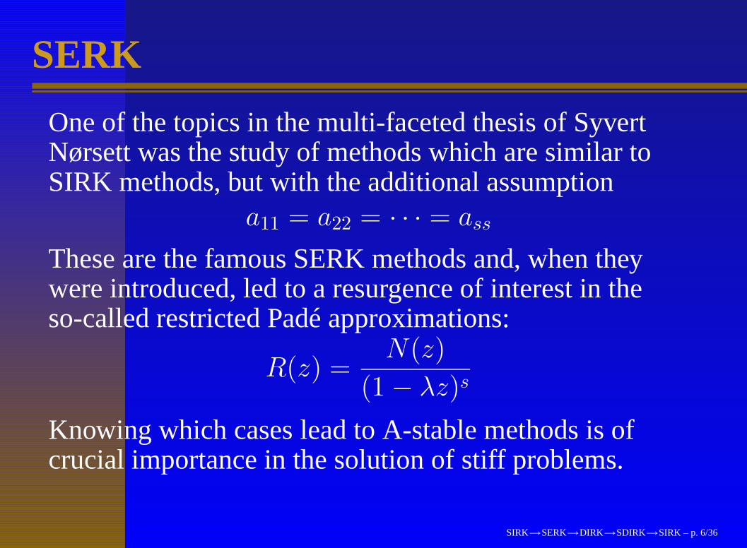
One of the topics in the multi-faceted thesis of SyvertNørsett was the study of methods which are similar toSIRK methods
, but with the additional assumptiona11 = a22 = · · · = ass
These are the famous SERK methods and, when theywere introduced, led to a resurgence of interest in theso-called restricted Padé approximations:
R(z) =N(z)
(1− λz)s
Knowing which cases lead to A-stable methods is ofcrucial importance in the solution of stiff problems.
SIRK→SERK→DIRK→SDIRK→SIRK – p. 6/36

SERK
One of the topics in the multi-faceted thesis of SyvertNørsett was the study of methods which are similar toSIRK methods, but with the additional assumption
a11 = a22 = · · · = ass
These are the famous SERK methods and, when theywere introduced, led to a resurgence of interest in theso-called restricted Padé approximations:
R(z) =N(z)
(1− λz)s
Knowing which cases lead to A-stable methods is ofcrucial importance in the solution of stiff problems.
SIRK→SERK→DIRK→SDIRK→SIRK – p. 6/36

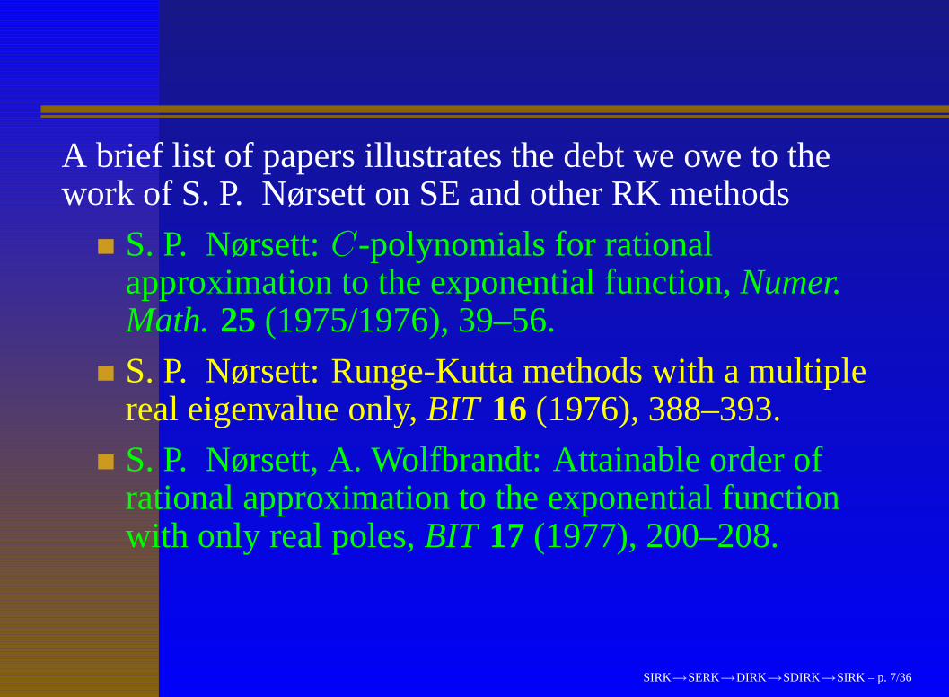
A brief list of papers illustrates the debt we owe to thework of S. P. Nørsett on SE and other RK methods
S. P. Nørsett: C-polynomials for rationalapproximation to the exponential function, Numer.Math. 25 (1975/1976), 39–56.
S. P. Nørsett: Runge-Kutta methods with a multiplereal eigenvalue only, BIT 16 (1976), 388–393.
S. P. Nørsett, A. Wolfbrandt: Attainable order ofrational approximation to the exponential functionwith only real poles, BIT 17 (1977), 200–208.
S. P. Nørsett: Restricted Padé approximations to theexponential function, SIAM J. Numer. Anal. 15(1978), 1008–1092.
SIRK→SERK→DIRK→SDIRK→SIRK – p. 7/36

DIRK
These methods with the acronym denotingDiagonally-Implicit Runge-Kutta methods were studiedby Roger Alexander.
The methods are just like SERKmethods and were developed independently.The following third order L-stable method illustrateswhat is possible for DIRK methods
λ λ12(1 + λ) 1
2(1− λ) λ
1 14(−6λ2 + 16λ− 1) 1
4(6λ2 − 20λ + 5) λ
14(−6λ2 + 16λ− 1) 1
4(6λ2 − 20λ + 5) λ
where λ ≈ 0.4358665215 satisfies 16−
32λ+3λ2−λ3 = 0.
SIRK→SERK→DIRK→SDIRK→SIRK – p. 8/36
DIRK
These methods with the acronym denotingDiagonally-Implicit Runge-Kutta methods were studiedby Roger Alexander. The methods are just like SERKmethods and were developed independently.
The following third order L-stable method illustrateswhat is possible for DIRK methods
λ λ12(1 + λ) 1
2(1− λ) λ
1 14(−6λ2 + 16λ− 1) 1
4(6λ2 − 20λ + 5) λ
14(−6λ2 + 16λ− 1) 1
4(6λ2 − 20λ + 5) λ
where λ ≈ 0.4358665215 satisfies 16−
32λ+3λ2−λ3 = 0.
SIRK→SERK→DIRK→SDIRK→SIRK – p. 8/36

DIRK
These methods with the acronym denotingDiagonally-Implicit Runge-Kutta methods were studiedby Roger Alexander. The methods are just like SERKmethods and were developed independently.The following third order L-stable method illustrateswhat is possible for DIRK methods
λ λ12(1 + λ) 1
2(1− λ) λ
1 14(−6λ2 + 16λ− 1) 1
4(6λ2 − 20λ + 5) λ
14(−6λ2 + 16λ− 1) 1
4(6λ2 − 20λ + 5) λ
where λ ≈ 0.4358665215 satisfies 16−
32λ+3λ2−λ3 = 0.
SIRK→SERK→DIRK→SDIRK→SIRK – p. 8/36

SDIRK
The change of name emphasised the singly-implicitnature of SDIRK methods
and seems to have been part ofan attempt at a systematic naming system.As we shallsee in the next few slides, singly-implicit methodswithout the DIRK structure are also possible.At least twopapers by the indomitable team of S. P. Nørsett andP. G. Thomsen have used the SDIRK name.
Embedded SDIRK methods of basic order three, BIT24 (1984), 364-646.
Local error control in SDIRK methods, BIT 26(1986), 100-113.
This work is part of a practical project to obtain efficientstiff solvers of moderate order.
SIRK→SERK→DIRK→SDIRK→SIRK – p. 9/36
SDIRK
The change of name emphasised the singly-implicitnature of SDIRK methods and seems to have been part ofan attempt at a systematic naming system.
As we shallsee in the next few slides, singly-implicit methodswithout the DIRK structure are also possible.At least twopapers by the indomitable team of S. P. Nørsett andP. G. Thomsen have used the SDIRK name.
Embedded SDIRK methods of basic order three, BIT24 (1984), 364-646.
Local error control in SDIRK methods, BIT 26(1986), 100-113.
This work is part of a practical project to obtain efficientstiff solvers of moderate order.
SIRK→SERK→DIRK→SDIRK→SIRK – p. 9/36
SDIRK
The change of name emphasised the singly-implicitnature of SDIRK methods and seems to have been part ofan attempt at a systematic naming system. As we shallsee in the next few slides, singly-implicit methodswithout the DIRK structure are also possible.
At least twopapers by the indomitable team of S. P. Nørsett andP. G. Thomsen have used the SDIRK name.
Embedded SDIRK methods of basic order three, BIT24 (1984), 364-646.
Local error control in SDIRK methods, BIT 26(1986), 100-113.
This work is part of a practical project to obtain efficientstiff solvers of moderate order.
SIRK→SERK→DIRK→SDIRK→SIRK – p. 9/36

SDIRK
The change of name emphasised the singly-implicitnature of SDIRK methods and seems to have been part ofan attempt at a systematic naming system. As we shallsee in the next few slides, singly-implicit methodswithout the DIRK structure are also possible. At leasttwo papers by the indomitable team of S. P. Nørsett andP. G. Thomsen have used the SDIRK name.
Embedded SDIRK methods of basic order three, BIT24 (1984), 364-646.
Local error control in SDIRK methods, BIT 26(1986), 100-113.
This work is part of a practical project to obtain efficientstiff solvers of moderate order.
SIRK→SERK→DIRK→SDIRK→SIRK – p. 9/36

SIRK
A SIRK method is characterised by the equationσ(A) = {λ}.
That is A has a one-point spectrum.
For DIRK methods the stages can be computedindependently and sequentiallyand each requiresapproximately the same factorised matrix I − hλJ topermit solution by a modified Newton iteration process.
How then is it possible to implement SIRK methods in asimilarly efficient manner?
The answer lies in the inclusion of a transformation toJordan canonical form into the computation.
SIRK→SERK→DIRK→SDIRK→SIRK – p. 10/36

SIRK
A SIRK method is characterised by the equationσ(A) = {λ}. That is A has a one-point spectrum.
For DIRK methods the stages can be computedindependently and sequentiallyand each requiresapproximately the same factorised matrix I − hλJ topermit solution by a modified Newton iteration process.
How then is it possible to implement SIRK methods in asimilarly efficient manner?
The answer lies in the inclusion of a transformation toJordan canonical form into the computation.
SIRK→SERK→DIRK→SDIRK→SIRK – p. 10/36
SIRK
A SIRK method is characterised by the equationσ(A) = {λ}. That is A has a one-point spectrum.
For DIRK methods the stages can be computedindependently and sequentially
and each requiresapproximately the same factorised matrix I − hλJ topermit solution by a modified Newton iteration process.
How then is it possible to implement SIRK methods in asimilarly efficient manner?
The answer lies in the inclusion of a transformation toJordan canonical form into the computation.
SIRK→SERK→DIRK→SDIRK→SIRK – p. 10/36

SIRK
A SIRK method is characterised by the equationσ(A) = {λ}. That is A has a one-point spectrum.
For DIRK methods the stages can be computedindependently and sequentially and each requiresapproximately the same factorised matrix I − hλJ topermit solution by a modified Newton iteration process.
How then is it possible to implement SIRK methods in asimilarly efficient manner?
The answer lies in the inclusion of a transformation toJordan canonical form into the computation.
SIRK→SERK→DIRK→SDIRK→SIRK – p. 10/36
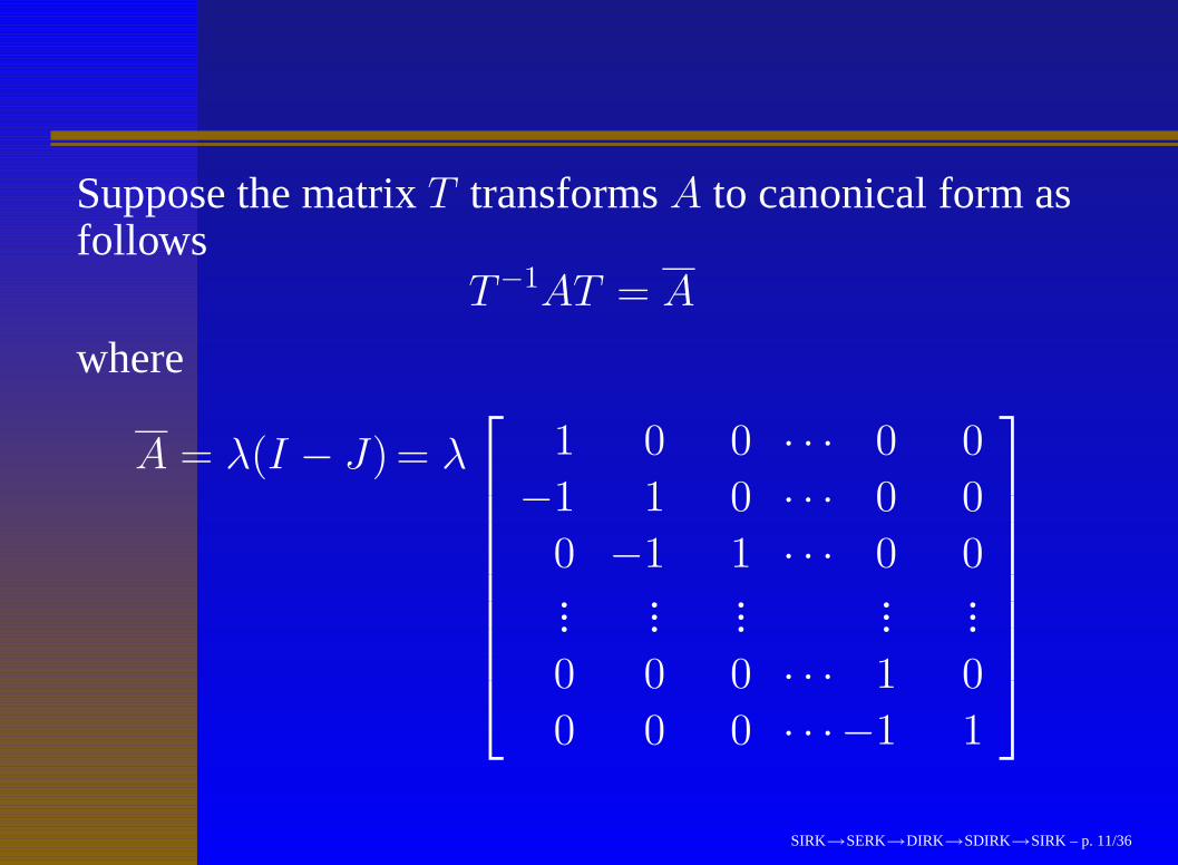
Suppose the matrix T transforms A to canonical form asfollows
T−1AT = A
where
A = λ(I − J) = λ
1 0 0 · · · 0 0
−1 1 0 · · · 0 0
0 −1 1 · · · 0 0... ... ... ... ...0 0 0 · · · 1 0
0 0 0 · · · −1 1
SIRK→SERK→DIRK→SDIRK→SIRK – p. 11/36

Suppose the matrix T transforms A to canonical form asfollows
T−1AT = A
where
A = λ(I − J)
= λ
1 0 0 · · · 0 0
−1 1 0 · · · 0 0
0 −1 1 · · · 0 0... ... ... ... ...0 0 0 · · · 1 0
0 0 0 · · · −1 1
SIRK→SERK→DIRK→SDIRK→SIRK – p. 11/36
Suppose the matrix T transforms A to canonical form asfollows
T−1AT = A
where
A = λ(I − J) = λ
1 0 0 · · · 0 0
−1 1 0 · · · 0 0
0 −1 1 · · · 0 0... ... ... ... ...0 0 0 · · · 1 0
0 0 0 · · · −1 1
SIRK→SERK→DIRK→SDIRK→SIRK – p. 11/36
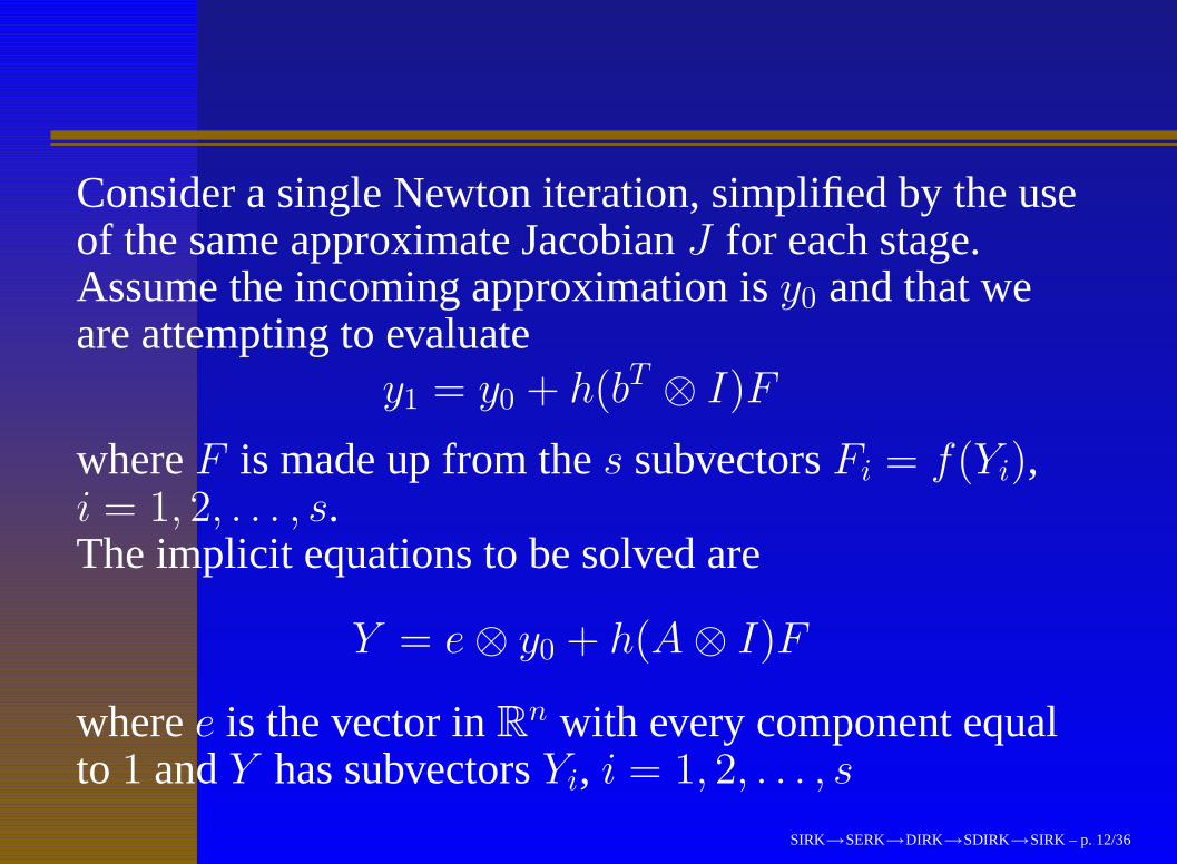
Consider a single Newton iteration, simplified by the useof the same approximate Jacobian J for each stage.
Assume the incoming approximation is y0 and that weare attempting to evaluate
y1 = y0 + h(bT ⊗ I)F
where F is made up from the s subvectors Fi = f(Yi),i = 1, 2, . . . , s.The implicit equations to be solved are
Y = e⊗ y0 + h(A⊗ I)F
where e is the vector in Rn with every component equal
to 1 and Y has subvectors Yi, i = 1, 2, . . . , s
SIRK→SERK→DIRK→SDIRK→SIRK – p. 12/36

Consider a single Newton iteration, simplified by the useof the same approximate Jacobian J for each stage.Assume the incoming approximation is y0 and that weare attempting to evaluate
y1 = y0 + h(bT ⊗ I)F
where F is made up from the s subvectors Fi = f(Yi),i = 1, 2, . . . , s.
The implicit equations to be solved are
Y = e⊗ y0 + h(A⊗ I)F
where e is the vector in Rn with every component equal
to 1 and Y has subvectors Yi, i = 1, 2, . . . , s
SIRK→SERK→DIRK→SDIRK→SIRK – p. 12/36

Consider a single Newton iteration, simplified by the useof the same approximate Jacobian J for each stage.Assume the incoming approximation is y0 and that weare attempting to evaluate
y1 = y0 + h(bT ⊗ I)F
where F is made up from the s subvectors Fi = f(Yi),i = 1, 2, . . . , s.The implicit equations to be solved are
Y = e⊗ y0 + h(A⊗ I)F
where e is the vector in Rn with every component equal
to 1 and Y has subvectors Yi, i = 1, 2, . . . , s
SIRK→SERK→DIRK→SDIRK→SIRK – p. 12/36

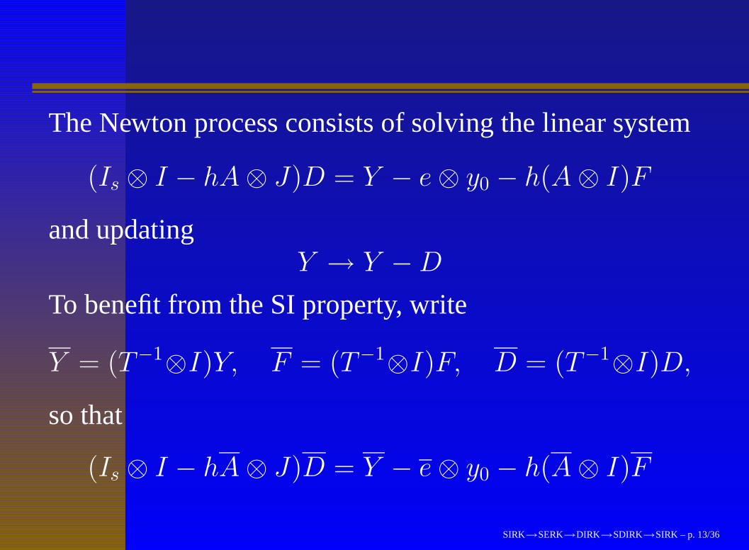
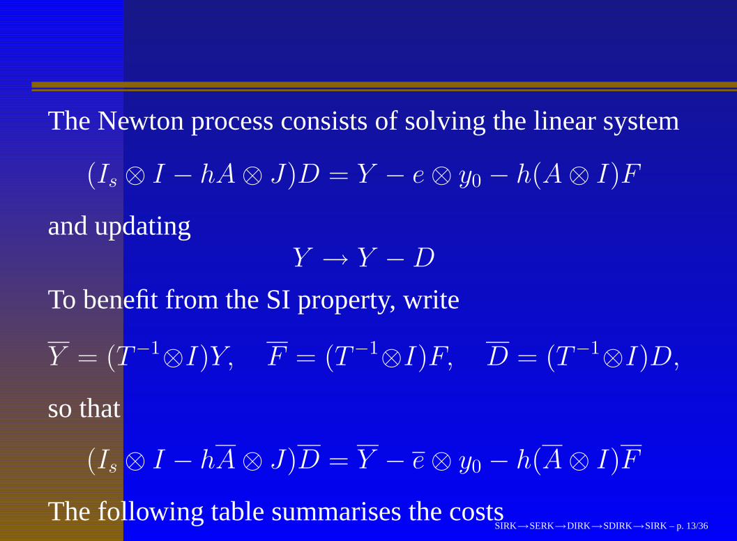
The Newton process consists of solving the linear system
(Is ⊗ I − hA⊗ J)D = Y − e⊗ y0 − h(A⊗ I)F
and updatingY → Y −D
To benefit from the SI property, write
Y = (T−1⊗I)Y, F = (T−1⊗I)F, D = (T−1⊗I)D,
so that
(Is ⊗ I − hA⊗ J)D = Y − e⊗ y0 − h(A⊗ I)F
The following table summarises the costs
SIRK→SERK→DIRK→SDIRK→SIRK – p. 13/36
The Newton process consists of solving the linear system
(Is ⊗ I − hA⊗ J)D = Y − e⊗ y0 − h(A⊗ I)F
and updatingY → Y −D
To benefit from the SI property, write
Y = (T−1⊗I)Y, F = (T−1⊗I)F, D = (T−1⊗I)D,
so that
(Is ⊗ I − hA⊗ J)D = Y − e⊗ y0 − h(A⊗ I)F
The following table summarises the costsSIRK→SERK→DIRK→SDIRK→SIRK – p. 13/36

without withtransformation transformation
LU factorisation s3N 3
N 3
Transformation s2N
Backsolves s2N 2
sN 2
Transformation s2N
In summary, we reduce the very high LU factorisationcostto a level comparable to BDF methods.
Also we reduce the back substitution costto the samework per stage as for DIRK or BDFmethods.
By comparison, the additional transformation costs areinsignificant for large problems .
SIRK→SERK→DIRK→SDIRK→SIRK – p. 14/36

without
with
transformation
transformation
LU factorisation s3N 3
N 3
Transformation s2N
Backsolves s2N 2
sN 2
Transformation s2N
In summary, we reduce the very high LU factorisationcostto a level comparable to BDF methods.
Also we reduce the back substitution costto the samework per stage as for DIRK or BDFmethods.
By comparison, the additional transformation costs areinsignificant for large problems .
SIRK→SERK→DIRK→SDIRK→SIRK – p. 14/36

without withtransformation transformation
LU factorisation s3N 3
N 3
Transformation s2N
Backsolves s2N 2
sN 2
Transformation s2N
In summary, we reduce the very high LU factorisationcostto a level comparable to BDF methods.
Also we reduce the back substitution costto the samework per stage as for DIRK or BDFmethods.
By comparison, the additional transformation costs areinsignificant for large problems .
SIRK→SERK→DIRK→SDIRK→SIRK – p. 14/36

without withtransformation transformation
LU factorisation s3N 3 N 3
Transformation s2N
Backsolves s2N 2 sN 2
Transformation s2N
In summary, we reduce the very high LU factorisationcost
to a level comparable to BDF methods.
Also we reduce the back substitution costto the samework per stage as for DIRK or BDFmethods.
By comparison, the additional transformation costs areinsignificant for large problems .
SIRK→SERK→DIRK→SDIRK→SIRK – p. 14/36

without withtransformation transformation
LU factorisation s3N 3 N 3
Transformation s2N
Backsolves s2N 2 sN 2
Transformation s2N
In summary, we reduce the very high LU factorisationcost to a level comparable to BDF methods
.
Also we reduce the back substitution costto the samework per stage as for DIRK or BDFmethods.
By comparison, the additional transformation costs areinsignificant for large problems .
SIRK→SERK→DIRK→SDIRK→SIRK – p. 14/36

without withtransformation transformation
LU factorisation s3N 3 N 3
Transformation s2N
Backsolves s2N 2 sN 2
Transformation s2N
In summary, we reduce the very high LU factorisationcost to a level comparable to BDF methods.
Also we reduce the back substitution cost
to the samework per stage as for DIRK or BDFmethods.
By comparison, the additional transformation costs areinsignificant for large problems .
SIRK→SERK→DIRK→SDIRK→SIRK – p. 14/36

without withtransformation transformation
LU factorisation s3N 3 N 3
Transformation s2N
Backsolves s2N 2 sN 2
Transformation s2N
In summary, we reduce the very high LU factorisationcost to a level comparable to BDF methods.
Also we reduce the back substitution cost to the samework per stage as for DIRK or BDF
methods.
By comparison, the additional transformation costs areinsignificant for large problems .
SIRK→SERK→DIRK→SDIRK→SIRK – p. 14/36

without withtransformation transformation
LU factorisation s3N 3 N 3
Transformation s2N
Backsolves s2N 2 sN 2
Transformation s2N
In summary, we reduce the very high LU factorisationcost to a level comparable to BDF methods.
Also we reduce the back substitution cost to the samework per stage as for DIRK or BDF methods.
By comparison, the additional transformation costs areinsignificant for large problems
.
SIRK→SERK→DIRK→SDIRK→SIRK – p. 14/36

without withtransformation transformation
LU factorisation s3N 3 N 3
Transformation s2N
Backsolves s2N 2 sN 2
Transformation s2N
In summary, we reduce the very high LU factorisationcost to a level comparable to BDF methods.
Also we reduce the back substitution cost to the samework per stage as for DIRK or BDF methods.
By comparison, the additional transformation costs areinsignificant for large problems .
SIRK→SERK→DIRK→SDIRK→SIRK – p. 14/36
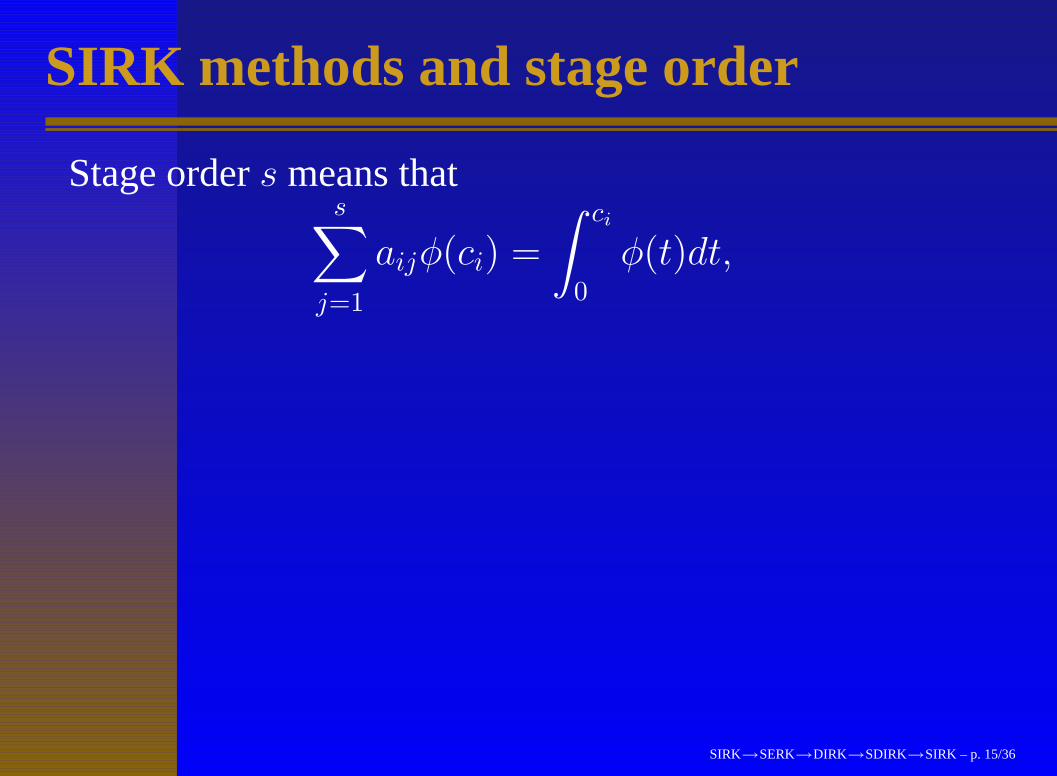
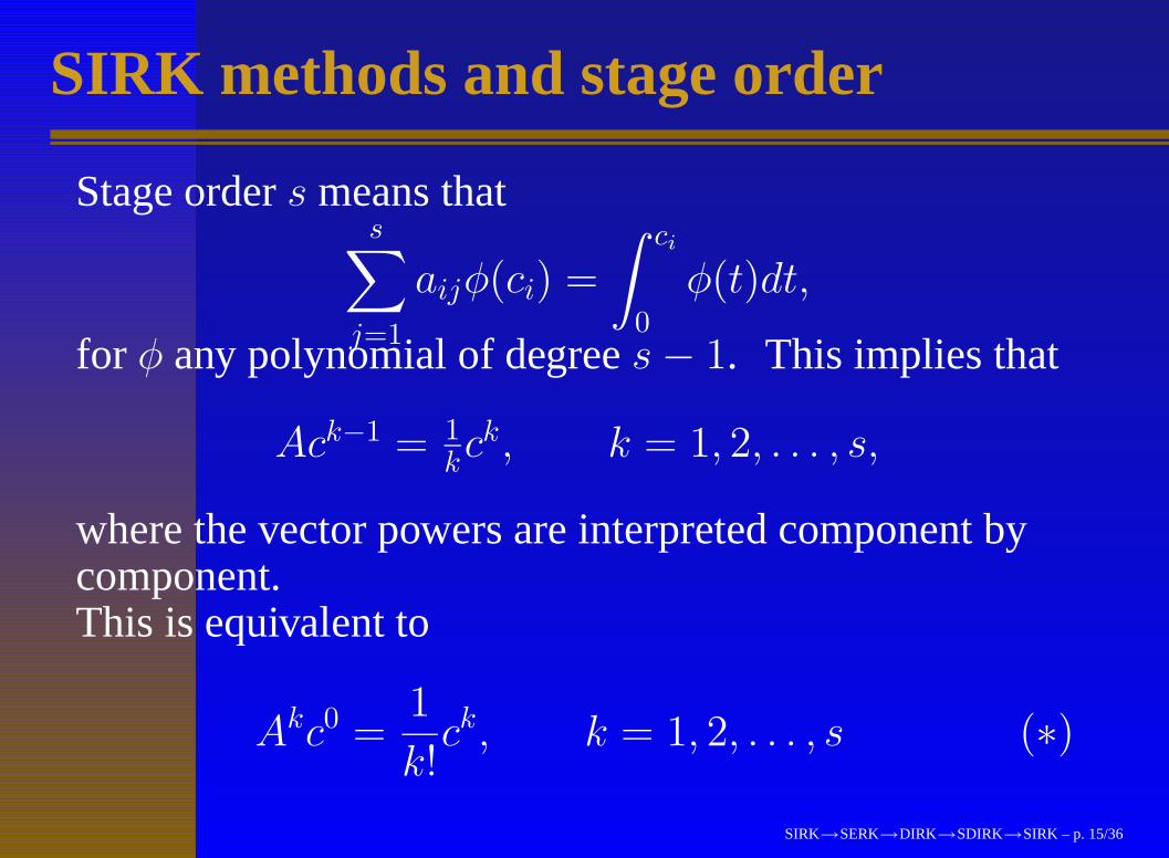
SIRK methods and stage order
Stage order s means thats∑
j=1
aijφ(ci) =
∫ ci
0
φ(t)dt,
for φ any polynomial of degree s− 1. This implies that
Ack−1 = 1kck, k = 1, 2, . . . , s,
where the vector powers are interpreted component bycomponent.This is equivalent to
Akc0 =1
k!ck, k = 1, 2, . . . , s (∗)
SIRK→SERK→DIRK→SDIRK→SIRK – p. 15/36

SIRK methods and stage order
Stage order s means thats∑
j=1
aijφ(ci) =
∫ ci
0
φ(t)dt,
for φ any polynomial of degree s− 1.
This implies that
Ack−1 = 1kck, k = 1, 2, . . . , s,
where the vector powers are interpreted component bycomponent.This is equivalent to
Akc0 =1
k!ck, k = 1, 2, . . . , s (∗)
SIRK→SERK→DIRK→SDIRK→SIRK – p. 15/36

SIRK methods and stage order
Stage order s means thats∑
j=1
aijφ(ci) =
∫ ci
0
φ(t)dt,
for φ any polynomial of degree s− 1. This implies that
Ack−1 = 1kck, k = 1, 2, . . . , s,
where the vector powers are interpreted component bycomponent.This is equivalent to
Akc0 =1
k!ck, k = 1, 2, . . . , s (∗)
SIRK→SERK→DIRK→SDIRK→SIRK – p. 15/36

SIRK methods and stage order
Stage order s means thats∑
j=1
aijφ(ci) =
∫ ci
0
φ(t)dt,
for φ any polynomial of degree s− 1. This implies that
Ack−1 = 1kck, k = 1, 2, . . . , s,
where the vector powers are interpreted component bycomponent.
This is equivalent to
Akc0 =1
k!ck, k = 1, 2, . . . , s (∗)
SIRK→SERK→DIRK→SDIRK→SIRK – p. 15/36
SIRK methods and stage order
Stage order s means thats∑
j=1
aijφ(ci) =
∫ ci
0
φ(t)dt,
for φ any polynomial of degree s− 1. This implies that
Ack−1 = 1kck, k = 1, 2, . . . , s,
where the vector powers are interpreted component bycomponent.This is equivalent to
Akc0 =1
k!ck, k = 1, 2, . . . , s (∗)
SIRK→SERK→DIRK→SDIRK→SIRK – p. 15/36

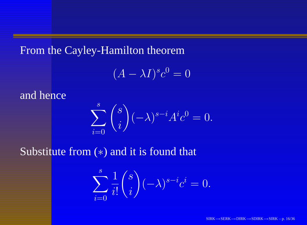
From the Cayley-Hamilton theorem
(A− λI)sc0 = 0
and hences∑
i=0
(s
i
)(−λ)s−iAic0 = 0.
Substitute from (∗) and it is found that
s∑
i=0
1
i!
(s
i
)(−λ)s−ici = 0.
SIRK→SERK→DIRK→SDIRK→SIRK – p. 16/36

From the Cayley-Hamilton theorem
(A− λI)sc0 = 0
and hences∑
i=0
(s
i
)(−λ)s−iAic0 = 0.
Substitute from (∗) and it is found that
s∑
i=0
1
i!
(s
i
)(−λ)s−ici = 0.
SIRK→SERK→DIRK→SDIRK→SIRK – p. 16/36
From the Cayley-Hamilton theorem
(A− λI)sc0 = 0
and hences∑
i=0
(s
i
)(−λ)s−iAic0 = 0.
Substitute from (∗) and it is found that
s∑
i=0
1
i!
(s
i
)(−λ)s−ici = 0.
SIRK→SERK→DIRK→SDIRK→SIRK – p. 16/36

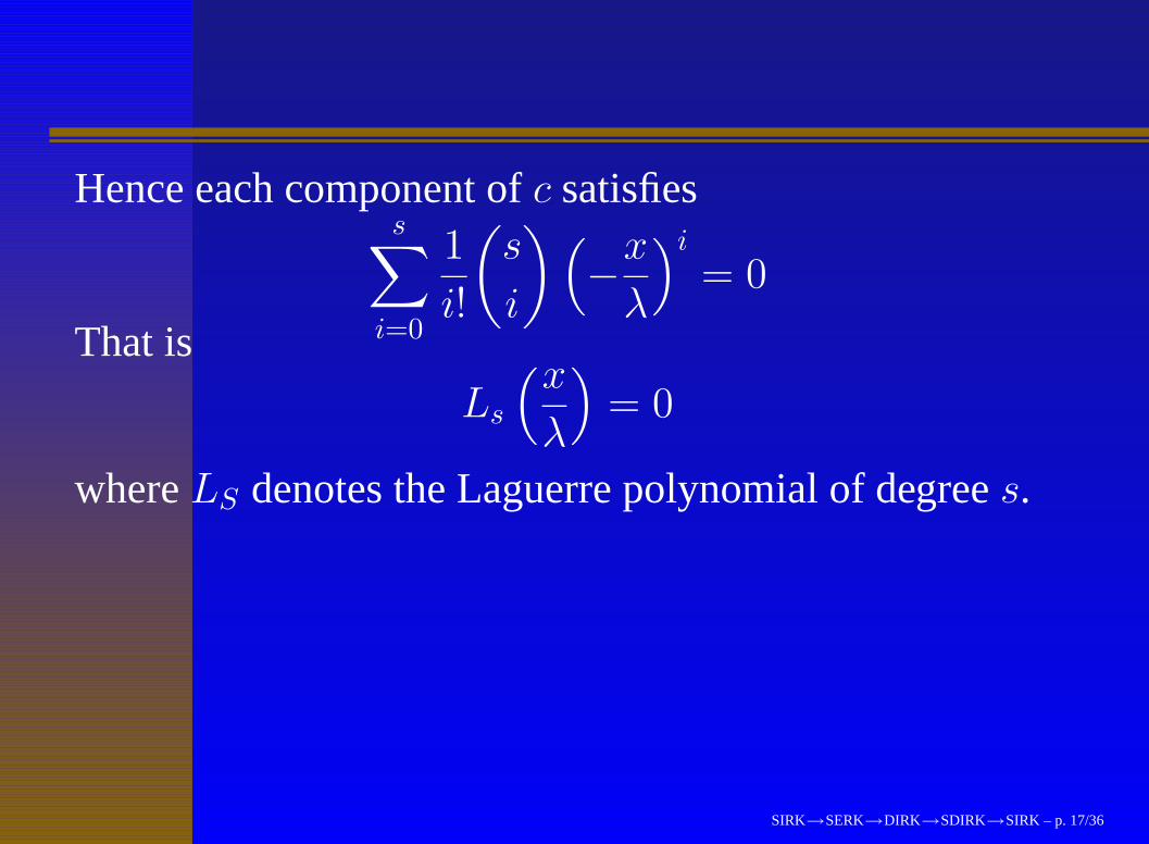
Hence each component of c satisfiess∑
i=0
1
i!
(s
i
)(−
x
λ
)i
= 0
That is
Ls
(x
λ
)= 0
where LS denotes the Laguerre polynomial of degree s.
Let ξ1, ξ2, . . . , ξs denote the zeros of Ls so that
ci = λξi, i = 1, 2, . . . , s
The question now is, how should λ be chosen?
SIRK→SERK→DIRK→SDIRK→SIRK – p. 17/36

Unfortunately, to obtain A-stability, at least for ordersp > 2, λ has to be chosen so that some of the ci areoutside the interval [0, 1].
This effect becomes more severe for increasingly highorders and can be seen as a major disadvantage of thesemethods.
We will look at two approaches for overcoming thisdisadvantage.
However, we first look at the transformation matrix T forefficient implementation.
SIRK→SERK→DIRK→SDIRK→SIRK – p. 18/36

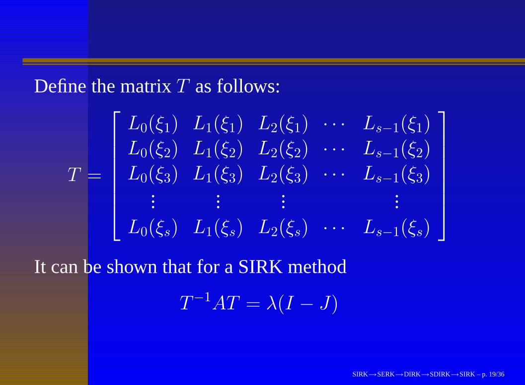
Define the matrix T as follows:
T =
L0(ξ1) L1(ξ1) L2(ξ1) · · · Ls−1(ξ1)
L0(ξ2) L1(ξ2) L2(ξ2) · · · Ls−1(ξ2)
L0(ξ3) L1(ξ3) L2(ξ3) · · · Ls−1(ξ3)... ... ... ...
L0(ξs) L1(ξs) L2(ξs) · · · Ls−1(ξs)
It can be shown that for a SIRK method
T−1AT = λ(I − J)
SIRK→SERK→DIRK→SDIRK→SIRK – p. 19/36
Define the matrix T as follows:
T =
L0(ξ1) L1(ξ1) L2(ξ1) · · · Ls−1(ξ1)
L0(ξ2) L1(ξ2) L2(ξ2) · · · Ls−1(ξ2)
L0(ξ3) L1(ξ3) L2(ξ3) · · · Ls−1(ξ3)... ... ... ...
L0(ξs) L1(ξs) L2(ξs) · · · Ls−1(ξs)
It can be shown that for a SIRK method
T−1AT = λ(I − J)
SIRK→SERK→DIRK→SDIRK→SIRK – p. 19/36
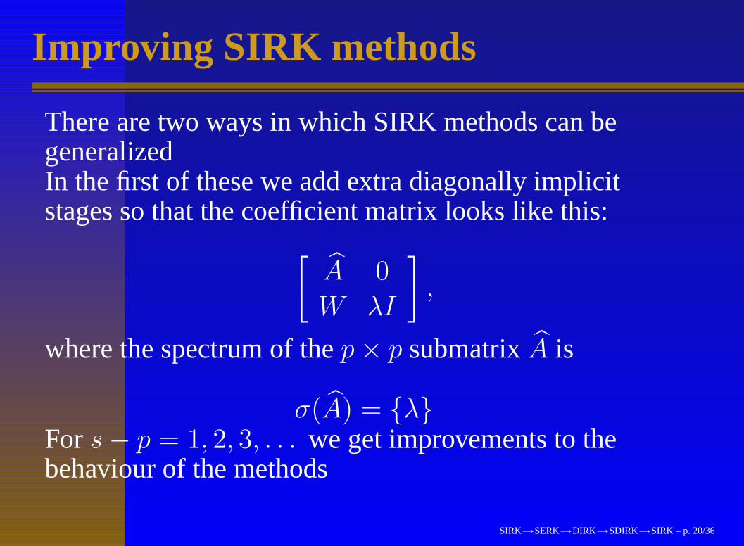
Improving SIRK methods
There are two ways in which SIRK methods can begeneralizedIn the first of these we add extra diagonally implicitstages so that the coefficient matrix looks like this:
[A 0
W λI
],
where the spectrum of the p× p submatrix A is
σ(A) = {λ}For s− p = 1, 2, 3, . . . we get improvements to thebehaviour of the methods
SIRK→SERK→DIRK→SDIRK→SIRK – p. 20/36

A second generalization is to replace “order” by“effective order”.
This allows us to locate the abscissae where we wish.
In “DESIRE” methods:Diagonally Extended Singly Implicit Runge-Kutta
methods using Effective orderthese two generalizations are combined.
We will examine effective order in more detail.
SIRK→SERK→DIRK→SDIRK→SIRK – p. 21/36

Doubly companion matrices
Matrices like the following are “companion matrices” forthe polynomial
zn + α1zn−1 + · · ·+ αn
orzn + β1z
n−1 + · · ·+ βn,
respectively:
−α1−α2−α3· · · −αn−1−αn
1 0 0 · · · 0 0
0 1 0 · · · 0 0... ... ... ... ...0 0 0 · · · 0 0
0 0 0 · · · 1 0
,
0 0 0 · · · 0 −βn
1 0 0 · · · 0 −βn−1
0 1 0 · · · 0 −βn−2... ... ... ... ...0 0 0 · · · 0 −β2
0 0 0 · · · 1 −β1
SIRK→SERK→DIRK→SDIRK→SIRK – p. 22/36

Doubly companion matrices
Matrices like the following are “companion matrices” forthe polynomial
zn + α1zn−1 + · · ·+ αnor
zn + β1zn−1 + · · ·+ βn,
respectively:
−α1−α2−α3· · · −αn−1−αn
1 0 0 · · · 0 0
0 1 0 · · · 0 0... ... ... ... ...0 0 0 · · · 0 0
0 0 0 · · · 1 0
,
0 0 0 · · · 0 −βn
1 0 0 · · · 0 −βn−1
0 1 0 · · · 0 −βn−2... ... ... ... ...0 0 0 · · · 0 −β2
0 0 0 · · · 1 −β1
SIRK→SERK→DIRK→SDIRK→SIRK – p. 22/36

Their characteristic polynomials can be found fromdet(I − zA) = α(z) or β(z), respectively, where,α(z) = 1+α1z+· · ·+αnz
n, β(z) = 1+β1z+· · ·+βnzn.
A matrix with both α and β terms:
X =
−α1 −α2 −α3 · · · −αn−1 −αn − βn
1 0 0 · · · 0 −βn−1
0 1 0 · · · 0 −βn−2... ... ... ... ...0 0 0 · · · 0 −β2
0 0 0 · · · 1 −β1
,
is known as a “doubly companion matrix” and hascharacteristic polynomial defined by
det(I − zX) = α(z)β(z) + O(zn+1)
SIRK→SERK→DIRK→SDIRK→SIRK – p. 23/36

Their characteristic polynomials can be found fromdet(I − zA) = α(z) or β(z), respectively, where,α(z) = 1+α1z+· · ·+αnz
n, β(z) = 1+β1z+· · ·+βnzn.
A matrix with both α and β terms:
X =
−α1 −α2 −α3 · · · −αn−1 −αn − βn
1 0 0 · · · 0 −βn−1
0 1 0 · · · 0 −βn−2... ... ... ... ...0 0 0 · · · 0 −β2
0 0 0 · · · 1 −β1
,
is known as a “doubly companion matrix”
and hascharacteristic polynomial defined by
det(I − zX) = α(z)β(z) + O(zn+1)
SIRK→SERK→DIRK→SDIRK→SIRK – p. 23/36

Their characteristic polynomials can be found fromdet(I − zA) = α(z) or β(z), respectively, where,α(z) = 1+α1z+· · ·+αnz
n, β(z) = 1+β1z+· · ·+βnzn.
A matrix with both α and β terms:
X =
−α1 −α2 −α3 · · · −αn−1 −αn − βn
1 0 0 · · · 0 −βn−1
0 1 0 · · · 0 −βn−2... ... ... ... ...0 0 0 · · · 0 −β2
0 0 0 · · · 1 −β1
,
is known as a “doubly companion matrix” and hascharacteristic polynomial defined by
det(I − zX) = α(z)β(z) + O(zn+1)SIRK→SERK→DIRK→SDIRK→SIRK – p. 23/36

Matrices Ψ−1 and Ψ transforming X to Jordan canonicalform are known.
In the special case of a single Jordan block with n-foldeigenvalue λ, we have
Ψ−1 =
1 λ + α1 λ2 + α1λ + α2 · · ·
0 1 2λ + α1 · · ·
0 0 1 · · ·... ... ... . . .
,
where row number i + 1 is formed from row number iby differentiating with respect to λ and dividing by i.
We have a similar expression for Ψ:
SIRK→SERK→DIRK→SDIRK→SIRK – p. 24/36

Matrices Ψ−1 and Ψ transforming X to Jordan canonicalform are known.
In the special case of a single Jordan block with n-foldeigenvalue λ, we have
Ψ−1 =
1 λ + α1 λ2 + α1λ + α2 · · ·
0 1 2λ + α1 · · ·
0 0 1 · · ·... ... ... . . .
,
where row number i + 1 is formed from row number i bydifferentiating with respect to λ and dividing by i.
We have a similar expression for Ψ:SIRK→SERK→DIRK→SDIRK→SIRK – p. 24/36
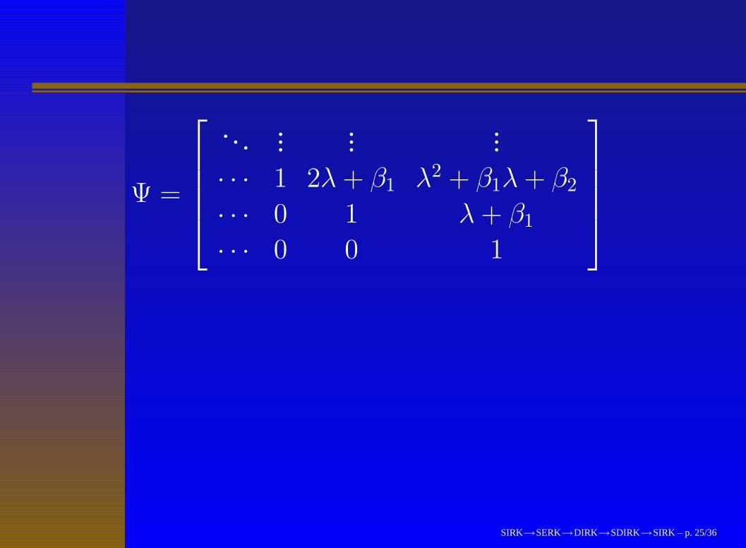
Ψ =
. . . ... ... ...· · · 1 2λ + β1 λ2 + β1λ + β2
· · · 0 1 λ + β1
· · · 0 0 1
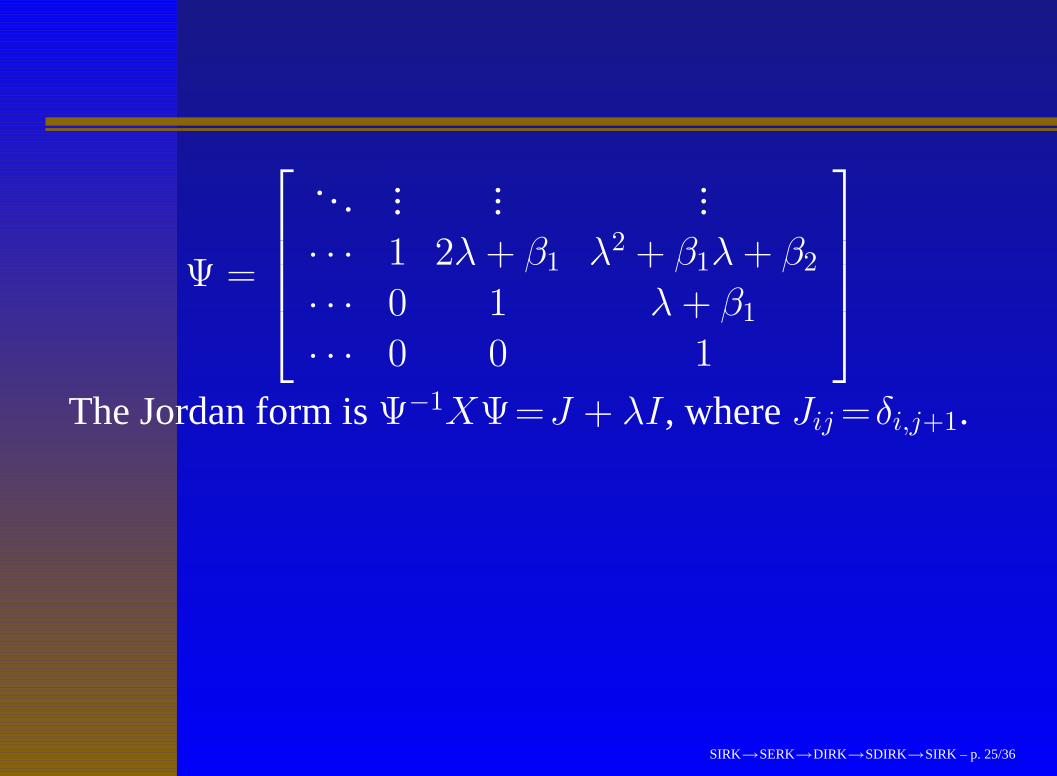
The Jordan form is Ψ−1XΨ=J + λI , where Jij =δi,j+1.That is
Ψ−1XΨ =
λ 0 · · · 0 0
1 λ · · · 0 0... ... ... ...0 0 · · · λ 0
0 0 · · · 1 λ
SIRK→SERK→DIRK→SDIRK→SIRK – p. 25/36
Ψ =
. . . ... ... ...· · · 1 2λ + β1 λ2 + β1λ + β2
· · · 0 1 λ + β1
· · · 0 0 1
The Jordan form is Ψ−1XΨ=J + λI , where Jij =δi,j+1.
That is
Ψ−1XΨ =
λ 0 · · · 0 0
1 λ · · · 0 0... ... ... ...0 0 · · · λ 0
0 0 · · · 1 λ
SIRK→SERK→DIRK→SDIRK→SIRK – p. 25/36

Ψ =
. . . ... ... ...· · · 1 2λ + β1 λ2 + β1λ + β2
· · · 0 1 λ + β1
· · · 0 0 1
The Jordan form is Ψ−1XΨ=J + λI , where Jij =δi,j+1.That is
Ψ−1XΨ =
λ 0 · · · 0 0
1 λ · · · 0 0... ... ... ...0 0 · · · λ 0
0 0 · · · 1 λ
SIRK→SERK→DIRK→SDIRK→SIRK – p. 25/36

Effective order
We will consider how to use the properties ofdoubly-companion matrices to derive SIRK methodswith effective order s.
First we look at the meaning of order for Runge-Kuttamethods and to its generalisation to effective order.
Denote by G the group consisting of mappings of(rooted) trees to real numbers where the group operationis defined in the usual way, according to the algebraictheory of Runge-Kutta methods or to the (equivalent)theory of B-series.
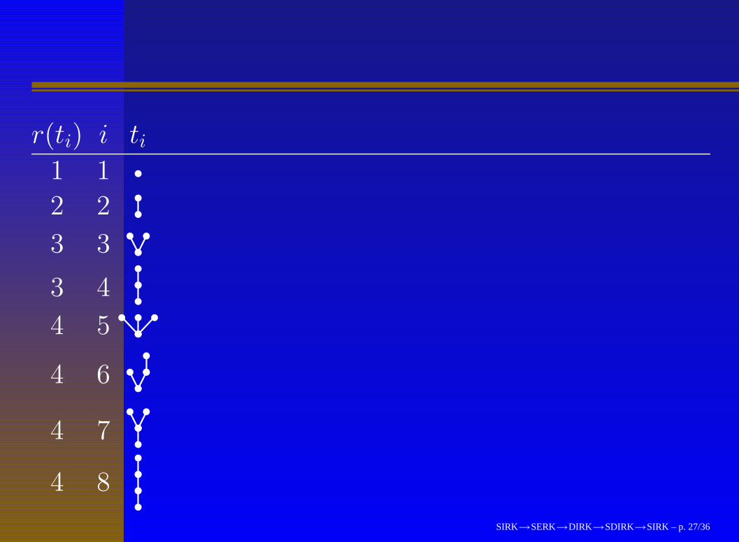
We will illustrate this operation in a table, where we alsointroduce the special member E ∈ G.
SIRK→SERK→DIRK→SDIRK→SIRK – p. 26/36

Effective order
We will consider how to use the properties ofdoubly-companion matrices to derive SIRK methodswith effective order s.
First we look at the meaning of order for Runge-Kuttamethods and to its generalisation to effective order.
Denote by G the group consisting of mappings of(rooted) trees to real numbers where the group operationis defined in the usual way, according to the algebraictheory of Runge-Kutta methods or to the (equivalent)theory of B-series.
We will illustrate this operation in a table, where we alsointroduce the special member E ∈ G.
SIRK→SERK→DIRK→SDIRK→SIRK – p. 26/36

Effective order
We will consider how to use the properties ofdoubly-companion matrices to derive SIRK methodswith effective order s.
First we look at the meaning of order for Runge-Kuttamethods and to its generalisation to effective order.
Denote by G the group consisting of mappings of(rooted) trees to real numbers where the group operationis defined in the usual way
, according to the algebraictheory of Runge-Kutta methods or to the (equivalent)theory of B-series.
We will illustrate this operation in a table, where we alsointroduce the special member E ∈ G.
SIRK→SERK→DIRK→SDIRK→SIRK – p. 26/36
Effective order
We will consider how to use the properties ofdoubly-companion matrices to derive SIRK methodswith effective order s.
First we look at the meaning of order for Runge-Kuttamethods and to its generalisation to effective order.
Denote by G the group consisting of mappings of(rooted) trees to real numbers where the group operationis defined in the usual way, according to the algebraictheory of Runge-Kutta methods or to the (equivalent)theory of B-series.
We will illustrate this operation in a table, where we alsointroduce the special member E ∈ G.
SIRK→SERK→DIRK→SDIRK→SIRK – p. 26/36

Effective order
We will consider how to use the properties ofdoubly-companion matrices to derive SIRK methodswith effective order s.
First we look at the meaning of order for Runge-Kuttamethods and to its generalisation to effective order.
Denote by G the group consisting of mappings of(rooted) trees to real numbers where the group operationis defined in the usual way, according to the algebraictheory of Runge-Kutta methods or to the (equivalent)theory of B-series.
We will illustrate this operation in a table
, where we alsointroduce the special member E ∈ G.
SIRK→SERK→DIRK→SDIRK→SIRK – p. 26/36

Effective order
We will consider how to use the properties ofdoubly-companion matrices to derive SIRK methodswith effective order s.
First we look at the meaning of order for Runge-Kuttamethods and to its generalisation to effective order.
Denote by G the group consisting of mappings of(rooted) trees to real numbers where the group operationis defined in the usual way, according to the algebraictheory of Runge-Kutta methods or to the (equivalent)theory of B-series.
We will illustrate this operation in a table, where we alsointroduce the special member E ∈ G.
SIRK→SERK→DIRK→SDIRK→SIRK – p. 26/36

r(ti)
i ti
α(ti) β(ti) (αβ)(ti) E(ti)
1
1
α1 β1 α1 + β1 1
2
2
α2 β2 α2 + α1β1 + β212
3
3
α3 β3 α3 + α21β1 + 2α1β2 + β3
13
3
4
α4 β4 α4 + α2β1 + α1β2 + β416
4
5
α5 β5 α5 + α31β1 + 3α2
1β2 + 3α1β3 + β514
4
6
α6 β6α6 + α1α2β1 + (α2
1 + α2)β2 18+ α1(β3 + β4) + β6
4
7
α7 β7 α7 + α3β1 + α21β2 + 2α1β4 + β7
112
4
8
α8 β8 α8 + α4β1 + α2β2 + α1β4 + β8124
SIRK→SERK→DIRK→SDIRK→SIRK – p. 27/36
r(ti) i ti
α(ti) β(ti) (αβ)(ti) E(ti)
1 1
α1 β1 α1 + β1 1
2 2
α2 β2 α2 + α1β1 + β212
3 3
α3 β3 α3 + α21β1 + 2α1β2 + β3
13
3 4
α4 β4 α4 + α2β1 + α1β2 + β416
4 5
α5 β5 α5 + α31β1 + 3α2
1β2 + 3α1β3 + β514
4 6
α6 β6α6 + α1α2β1 + (α2
1 + α2)β2 18+ α1(β3 + β4) + β6
4 7
α7 β7 α7 + α3β1 + α21β2 + 2α1β4 + β7
112
4 8
α8 β8 α8 + α4β1 + α2β2 + α1β4 + β8124
SIRK→SERK→DIRK→SDIRK→SIRK – p. 27/36

r(ti) i ti α(ti) β(ti)
(αβ)(ti) E(ti)
1 1 α1 β1
α1 + β1 1
2 2 α2 β2
α2 + α1β1 + β212
3 3 α3 β3
α3 + α21β1 + 2α1β2 + β3
13
3 4 α4 β4
α4 + α2β1 + α1β2 + β416
4 5 α5 β5
α5 + α31β1 + 3α2
1β2 + 3α1β3 + β514
4 6 α6 β6
α6 + α1α2β1 + (α21 + α2)β2 1
8+ α1(β3 + β4) + β6
4 7 α7 β7
α7 + α3β1 + α21β2 + 2α1β4 + β7
112
4 8 α8 β8
α8 + α4β1 + α2β2 + α1β4 + β8124
SIRK→SERK→DIRK→SDIRK→SIRK – p. 27/36

r(ti) i ti α(ti) β(ti) (αβ)(ti)
E(ti)
1 1 α1 β1 α1 + β1
1
2 2 α2 β2 α2 + α1β1 + β2
12
3 3 α3 β3 α3 + α21β1 + 2α1β2 + β3
13
3 4 α4 β4 α4 + α2β1 + α1β2 + β4
16
4 5 α5 β5 α5 + α31β1 + 3α2
1β2 + 3α1β3 + β5
14
4 6 α6 β6α6 + α1α2β1 + (α2
1 + α2)β2
18
+ α1(β3 + β4) + β6
4 7 α7 β7 α7 + α3β1 + α21β2 + 2α1β4 + β7
112
4 8 α8 β8 α8 + α4β1 + α2β2 + α1β4 + β8
124
SIRK→SERK→DIRK→SDIRK→SIRK – p. 27/36

r(ti) i ti α(ti) β(ti) (αβ)(ti) E(ti)
1 1 α1 β1 α1 + β1 1
2 2 α2 β2 α2 + α1β1 + β212
3 3 α3 β3 α3 + α21β1 + 2α1β2 + β3
13
3 4 α4 β4 α4 + α2β1 + α1β2 + β416
4 5 α5 β5 α5 + α31β1 + 3α2
1β2 + 3α1β3 + β514
4 6 α6 β6α6 + α1α2β1 + (α2
1 + α2)β2 18+ α1(β3 + β4) + β6
4 7 α7 β7 α7 + α3β1 + α21β2 + 2α1β4 + β7
112
4 8 α8 β8 α8 + α4β1 + α2β2 + α1β4 + β8124
SIRK→SERK→DIRK→SDIRK→SIRK – p. 27/36

Gp will denote the normal subgroup defined by t 7→ 0 forr(t) ≤ p.
If α ∈ G then this maps canonically to αGp ∈ G/Gp.
If α is defined from the elementary weights for aRunge-Kutta method then order p can be written as
αGp = EGp.
Effective order p is defined by the existence of β suchthat
βαGp = EβGp.
SIRK→SERK→DIRK→SDIRK→SIRK – p. 28/36

The computational interpretation of this idea is that wecarry out a starting step corresponding to β
and afinishing step corresponding to β−1, with many steps inbetween corresponding to α.
This is equivalent to many steps all corresponding toβαβ−1.
Thus, the benefits of high order can be enjoyed by higheffective order.
SIRK→SERK→DIRK→SDIRK→SIRK – p. 29/36

The computational interpretation of this idea is that wecarry out a starting step corresponding to β and afinishing step corresponding to β−1
, with many steps inbetween corresponding to α.
This is equivalent to many steps all corresponding toβαβ−1.
Thus, the benefits of high order can be enjoyed by higheffective order.
SIRK→SERK→DIRK→SDIRK→SIRK – p. 29/36

The computational interpretation of this idea is that wecarry out a starting step corresponding to β and afinishing step corresponding to β−1, with many steps inbetween corresponding to α.
This is equivalent to many steps all corresponding toβαβ−1.
Thus, the benefits of high order can be enjoyed by higheffective order.
SIRK→SERK→DIRK→SDIRK→SIRK – p. 29/36

We analyse the conditions for effective order 4.
Without loss of generality assume β(t1) = 0.i (βα)(ti) (Eβ)(ti)
1 α1 1
2 β2 + α212 + β2
3 β3 + α313 + 2β2 + β3
4 β4 + β2α1 + α416 + β2 + β4
5 β5 + α514 + 3β2 + 3β3 + β5
6 β6 + β2α2 + α618 + 3
2β2 + β3 + β4 + β6
7 β7 + β3α1 + α7112 + β2 + 2β4 + β7
8 β8 + β4α1 + β2α2 + α8124 + 1
2β2 + β4 + β8
SIRK→SERK→DIRK→SDIRK→SIRK – p. 30/36

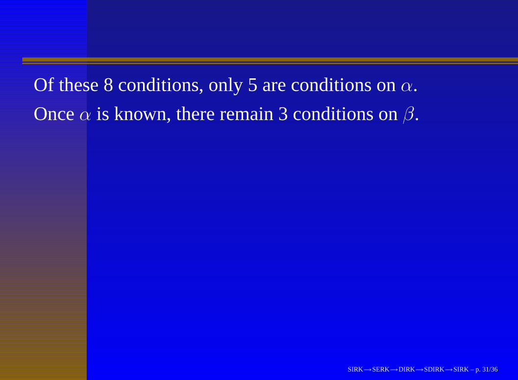
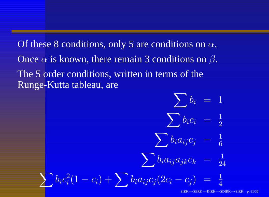
Of these 8 conditions, only 5 are conditions on α.
Once α is known, there remain 3 conditions on β.
The 5 order conditions, written in terms of theRunge-Kutta tableau, are ∑
bi = 1∑
bici = 12∑
biaijcj = 16∑
biaijajkck = 124∑
bic2i (1− ci) +
∑biaijcj(2ci − cj) = 1
4
SIRK→SERK→DIRK→SDIRK→SIRK – p. 31/36
Of these 8 conditions, only 5 are conditions on α.
Once α is known, there remain 3 conditions on β.
The 5 order conditions, written in terms of theRunge-Kutta tableau, are ∑
bi = 1∑
bici = 12∑
biaijcj = 16∑
biaijajkck = 124∑
bic2i (1− ci) +
∑biaijcj(2ci − cj) = 1
4SIRK→SERK→DIRK→SDIRK→SIRK – p. 31/36

Effective order of SIRK methods
If the stage order is equal to the order, then this analysiscan be simplified.
We can assume the input to step n is an approximation to
y(xn−1) + α1hy′(xn−1) + · · ·+ αshsy(s)(xn−1)
and we want the output to be an approximation to
y(xn) + α1hy′(xn) + · · ·+ αshsy(s)(xn)
To construct a SIRK method with effective order s, andwith a specific choice of the abscissa vector c and aspecific value of λ, use the properties of doublycompanion matrices.
SIRK→SERK→DIRK→SDIRK→SIRK – p. 32/36

Effective order of SIRK methods
If the stage order is equal to the order, then this analysiscan be simplified.We can assume the input to step n is an approximation to
y(xn−1) + α1hy′(xn−1) + · · ·+ αshsy(s)(xn−1)
and we want the output to be an approximation to
y(xn) + α1hy′(xn) + · · ·+ αshsy(s)(xn)
To construct a SIRK method with effective order s, andwith a specific choice of the abscissa vector c and aspecific value of λ, use the properties of doublycompanion matrices.
SIRK→SERK→DIRK→SDIRK→SIRK – p. 32/36

Construction of methods
Choose λ and abscissa vector c.
Define β1, β2, . . . , βs so that the zeros of thepolynomial
1s!x
s + β1
(s−1)!xs−1 + · · ·+ βs
are c1, c2, . . . cs.
Define α1, α2, . . . , αs so thatα(z)β(z) = (1− λz)s + O(zs+1)
Construct the corresponding doubly companionmatrix X
SIRK→SERK→DIRK→SDIRK→SIRK – p. 33/36
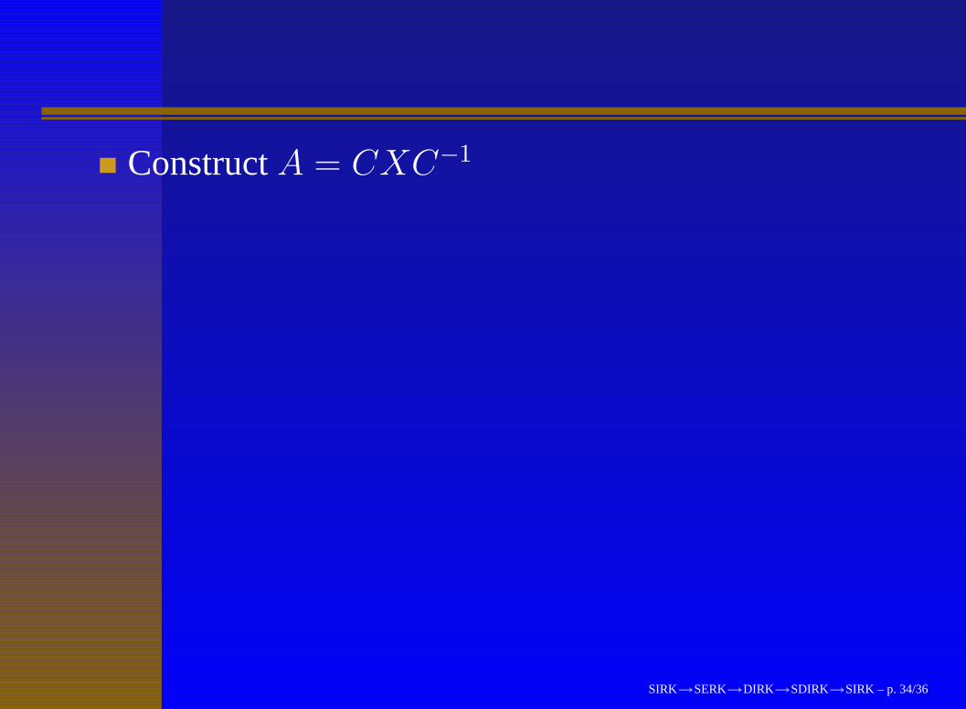
Construct A = CXC−1
, where
C =
1 c112!c
21 · · · 1
(s−1)!cs−11
1 c212!c
22 · · · 1
(s−1)!cs−12
... ... ... ...1 cs
12!c
2s · · · 1
(s−1)!cs−1s
Construct bT = bTC−1, where
bT =[
11! ,
α1
1! + 12! ,
α2
1! + α1
2! + 13! , . . . , αs−1
1! + · · ·+ 1s!
]
SIRK→SERK→DIRK→SDIRK→SIRK – p. 34/36

Construct A = CXC−1, where
C =
1 c112!c
21 · · · 1
(s−1)!cs−11
1 c212!c
22 · · · 1
(s−1)!cs−12
... ... ... ...1 cs
12!c
2s · · · 1
(s−1)!cs−1s
Construct bT = bTC−1, where
bT =[
11! ,
α1
1! + 12! ,
α2
1! + α1
2! + 13! , . . . , αs−1
1! + · · ·+ 1s!
]
SIRK→SERK→DIRK→SDIRK→SIRK – p. 34/36

Construct A = CXC−1, where
C =
1 c112!c
21 · · · 1
(s−1)!cs−11
1 c212!c
22 · · · 1
(s−1)!cs−12
... ... ... ...1 cs
12!c
2s · · · 1
(s−1)!cs−1s
Construct bT = bTC−1
, where
bT =[
11! ,
α1
1! + 12! ,
α2
1! + α1
2! + 13! , . . . , αs−1
1! + · · ·+ 1s!
]
SIRK→SERK→DIRK→SDIRK→SIRK – p. 34/36

Construct A = CXC−1, where
C =
1 c112!c
21 · · · 1
(s−1)!cs−11
1 c212!c
22 · · · 1
(s−1)!cs−12
... ... ... ...1 cs
12!c
2s · · · 1
(s−1)!cs−1s
Construct bT = bTC−1, where
bT =[
11! ,
α1
1! + 12! ,
α2
1! + α1
2! + 13! , . . . , αs−1
1! + · · ·+ 1s!
]
SIRK→SERK→DIRK→SDIRK→SIRK – p. 34/36

Final comments
The search for efficient methods to solve stiffproblems requires a balance between three aims:
accuracy, stability, low cost
A good place to look for these methods is amongstSERK methods and their generalisations
Further generalisations are also possible
The development of stiff methods is inextricablylinked with the pioneering work of S. P. Nørsett
I am greatly honoured to be present at thiscelebration of his outstanding contributions
Lastly: I will report on my efforts to document linksbetween the two of us
SIRK→SERK→DIRK→SDIRK→SIRK – p. 35/36

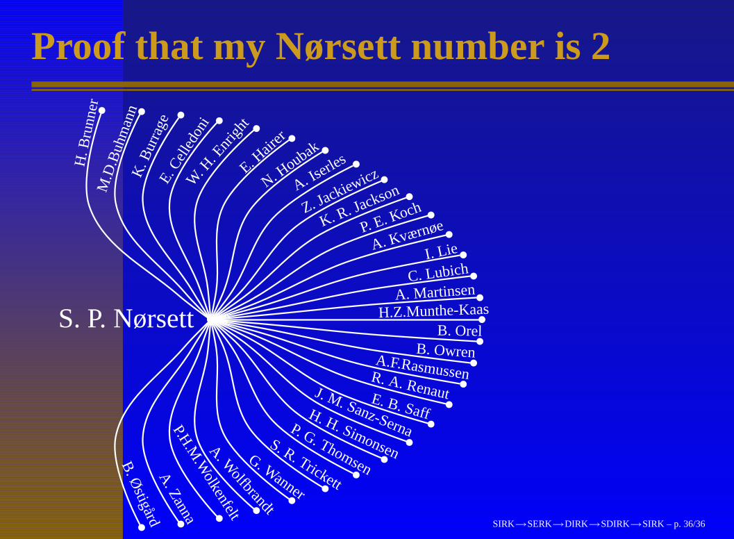
Proof that my Nørsett number is 2
S. P. Nørsett
H. B
runn
erM
.D.B
uhm
ann
K. B
urra
geE.
Celle
doni
W. H
. Enr
ight
E. Hair
er
N. Houbak
A. Iserles
Z. Jackiewicz
K. R. Jackson
P. E. Koch
A. Kværnøe
I. Lie
C. Lubich
A. Martinsen
H.Z.Munthe-KaasB. Orel
B. OwrenA.F.RasmussenR. A. RenautE. B. Saff
J. M. Sanz-SernaH. H. Simonsen
P. G. Thomsen
S. R. Trickett
G. Wanner
A. Wolfbrandt
P.H.M
.Wolkenfelt
A. Zanna
B. Ø
stigård
J. C. B.
SIRK→SERK→DIRK→SDIRK→SIRK – p. 36/36