Sede Amministrativa: Universita degli Studi de PadovaDipartimento di Matematica

DOTTORATO DI RICERCA IN MATEMATICAINDIRIZZO: MATEMATICACICLO XXVII

Singular Perturbations and Ergodic Problems fordegenerate parabolic Bellman PDEs in Rm with

Unbounded Data

Direttore della Scuola: Ch.mo Prof. Pierpaolo Soravia

Coordinatore d’indirizzo: Ch.mo Prof. Franco Cardin

Supervisore: Ch.mo Prof. Martino Bardi

Dottorando: Joao Henrique Branco Meireles

Luglio 2015

Acknowledgements

I would like to thank my advisor Professor Martino Bardi for introduc-ing me to the worlds of Singular Perturbation Theory, Homogenisation ofnonlinear PDEs and Ergodic Control Problems and for his guidance andvaluable suggestions that were a constant in our meetings. Professor GuyBarles deserves a special place. This work is deeply influenced by many pro-ductive discussions with him - without them, many of these results will notbe achieved. To both my full gratitude.

I would like also to thank my closest friends Ana Borges, Vanessa Vieira,David Fable, Ferdinando Pozzato and Mauro Tosato. Special thanks go toIgor Dzvinchuk.

Finally, but not least important, I would like to thank my parents, brother,sister and grandparents for all their love and constant backing. I’m fortunateto have all of them. Thank you!

ii

Resume

In this thesis we treat the first singular perturbation problem of a stochas-tic model with unbounded and controlled fast variables with success. Ourmethods are based on the theory of viscosity solutions, homogenisation offully nonlinear PDEs and a careful analysis of the associated ergodic stochas-tic control problem in the whole space Rm. The text is divided in two parts.

In the first chapter, we investigate the existence and uniqueness as wellas a suitable stability of the solution to the associated ergodic problem thatare crucial to characterize the effective Hamiltonian of the limit (effective)Cauchy problem in Chapter II of this thesis. The main achievement obtainedin this part is a purely analytical proof for the uniqueness of solution to suchergodic problem. Since the state space of the problem is not compact, ingeneral there are infinitely many solutions to the ergodic problem. However,if one restrict the class of solutions to the set of bounded-below functions,then it is known that uniqueness holds up to an additive constant. Theexisting proof relies on some probabilistic techniques employing the invariantprobability measure for the associated stochastic process. Here we give a newproof, purely analytic, based on the strong maximum principle. We believethat our results can be interesting and useful for researchers in the PDEcommunity.

In the second chapter, we introduce our singular perturbation model ofa stochastic control problem and we prove our main result: the convergenceof the value function V ε associated to the problem to the solution of thelimiting equation. More precisely, we prove that the functions

V (t, x) := lim inf(ε,t′,x′)→(0,t,x)

infy∈Rm

V ε(t′, x′, y)

and

V (t, x) := (supRVR)∗(t, x) (upper semi-continuous envelope of sup

RVR )

where VR(t, x) := lim sup(ε,t′,x′)→(0,t,x) supy∈BR(0) Vε(t′, x′, y), are, respectively,

a super and a subsolution of the effective Cauchy problem. As a corollary ofthis result, V ε converges to the unique solution V of the effective equationprovided the equation admits the comparison principle for discontinuous vis-cosity solutions. The justification of this convergence is not trivial at all. Itespecially involves some regularity issues and a careful treatment of viscos-ity techniques and stochastic analysis. This result has never been obtained

iii

before.

Key words: Singular perturbations, viscosity solutions, optimal stochas-tic control problems, ergodic control problems in the whole space Rm, PDEs

iv

Riassunto

In questa tesi viene trattato con successo il primo problema di pertur-bazione singolare di un modello stocastico con variabili veloci controllatee non limitate. I metodi si basano sulla teoria delle soluzioni di viscosita,omogeinizzazione dei PDE completamente non lineari, e su un’attenta anal-isi del problema stocastico ergodico associato, valido nell’intero spazio Rm.Il testo e diviso in due parti.

Nel primo capitolo, saranno studiate l’esistenza, l’unicita e alcune pro-prieta di stabilita della soluzione del problema ergodico, riferito sopra, chesono essenziali per caratterizzare il Hamiltoniano effetivo che appare in unProblema di Cauchy “limite”, che sara descritto nel capitolo II di questatesi. Il principale contributo, presentato in questa parte, e una prova pu-ramente analitica dell’unicita della soluzione di questo problema ergodico.Siccome lo stato dello spazio del problema non e compatto, in generale cisono un numero infinito di soluzioni a questo problema. Tuttavia, se unolimitasse la classe di soluzioni all’insieme di funzioni limitate inferiormente,allora e noto che l’unicita sara mantenuta a meno di una costante. La provaesistente si basa su alcune tecniche probabilistiche che impiegano la misuradi probabilta inviariante per l’associato processo stocastico. Qua verra datauna nuova prova, puramente analitica, basata sul principio del massimo. Siritiene che il risultato potra essere interessante ed utile per i ricercatori chelavorano all’interno della comunita di ricerca delle Equazioni Differenziali allederivate Parziali (PDE).

Nel secondo capitolo, sara introdotto un modello di perturbazione singo-lare di un problema di controllo stocastico, e provato il risultato principale:la convergenza della funzione valore V ε, associata al nostro problema, persoluzione dell’equazione limite . Piu precisamente, sara provato che le fun-zioni:

V (t, x) := lim inf(ε,t′,x′)→(0,t,x)

infy∈Rm

V ε(t′, x′, y)

e

V (t, x) := (supRVR)∗(t, x) (upper semi-continuous envelope of sup

RVR )

dove VR(t, x) := lim sup(ε,t′,x′)→(0,t,x) supy∈BR(0) Vε(t′, x′, y), sono, rispettiva-

mente, una super soluzione e una sottosoluzione del problema effettivo diCauchy. Come corollario di questo risultato, V ε converge all’unica soluzioneV della equazione effettiva se l’equazione limite permette il principio di com-parazione per le soluzioni di viscosita discontinue. La motivazione di questa

v

convergenza non e ovvia del tutto. Coinvolge specialmente alcuni problemidi regolarita e un trattamento attento delle tecniche di viscosita e di analisistocastica. Questo risultato e nuovo e non e mai stato ottenuto, prima d’ora,in la letteratura Matematica.

Parole chiave: Perturbazioni singolari, soluzioni di viscosita, problemi dicontrollo stocastico ottimale, problemi di controllo ergodico nello spazio Rm,equazioni differenziali alle derivate parziali.

vi

Contents

Introduction ix

Chapter I - The Ergodic Problem 1

Part I - Existence 3

1 Solvability of (EP ) 41.1 Functions φβ . . . . . . . . . . . . . . . . . . . . . . . . . . . . 51.2 Existence of solutions for (EP ) . . . . . . . . . . . . . . . . . 61.3 Infinite number of solutions . . . . . . . . . . . . . . . . . . . 81.4 Existence of a critical value . . . . . . . . . . . . . . . . . . . 9

2 Bounded from below solutions of (EP ) 122.1 Estimate for solutions of (EP ) . . . . . . . . . . . . . . . . . . 122.2 The class Φβ . . . . . . . . . . . . . . . . . . . . . . . . . . . . 132.3 Existence of a solution of (EP ) in Φβ . . . . . . . . . . . . . . 13

3 Approximations 193.1 Subquadratic and quadratic cases . . . . . . . . . . . . . . . . 193.2 Superquadratic case . . . . . . . . . . . . . . . . . . . . . . . . 21

Part II - Uniqueness 23

4 Uniqueness 244.1 Superquadratic and quadratic cases . . . . . . . . . . . . . . . 24

4.1.1 Transformation z = −e−φ . . . . . . . . . . . . . . . . 244.1.2 The Strong Maximum Principle . . . . . . . . . . . . . 314.1.3 Uniqueness of (EP ) . . . . . . . . . . . . . . . . . . . . 32

4.2 Sub quadratic case . . . . . . . . . . . . . . . . . . . . . . . . 344.2.1 Behaviour at infinity of the solutions of the ergodic

problem . . . . . . . . . . . . . . . . . . . . . . . . . . 344.2.2 Uniqueness of (EP ) . . . . . . . . . . . . . . . . . . . . 36

4.3 Conclusion . . . . . . . . . . . . . . . . . . . . . . . . . . . . . 38

Part III - Consequences of the Uniqueness 39

5 Remark on the properties of λ 40

6 Approximations of (EP ) 446.1 Convergence of approximations to (EP ) by perturbations of f 446.2 Convergence of approximations to (EP ) by restrictions to balls 46

vii

Chapter II - The Singular Perturbation Problem 49

7 The stochastic control system 517.1 The two-scale system . . . . . . . . . . . . . . . . . . . . . . . 517.2 The optimal control problem . . . . . . . . . . . . . . . . . . . 537.3 The HJB equation . . . . . . . . . . . . . . . . . . . . . . . . 53

8 The Cauchy Problem for the HJB equation 568.1 Assumptions . . . . . . . . . . . . . . . . . . . . . . . . . . . . 568.2 A subsolution and a supersolution for V ε . . . . . . . . . . . . 578.3 Well posedness . . . . . . . . . . . . . . . . . . . . . . . . . . 64

9 The effective Hamiltonian 699.1 The effective Hamiltonian . . . . . . . . . . . . . . . . . . . . 699.2 The standing assumptions . . . . . . . . . . . . . . . . . . . . 709.3 Some results for H . . . . . . . . . . . . . . . . . . . . . . . . 71

10 Convergence theorem 7310.1 Convergence theorem . . . . . . . . . . . . . . . . . . . . . . . 7310.2 Examples . . . . . . . . . . . . . . . . . . . . . . . . . . . . . 87

Appendix A - Some Stochastic Results 91

Appendix B - Gradient Estimate 95

Bibliography 97

viii

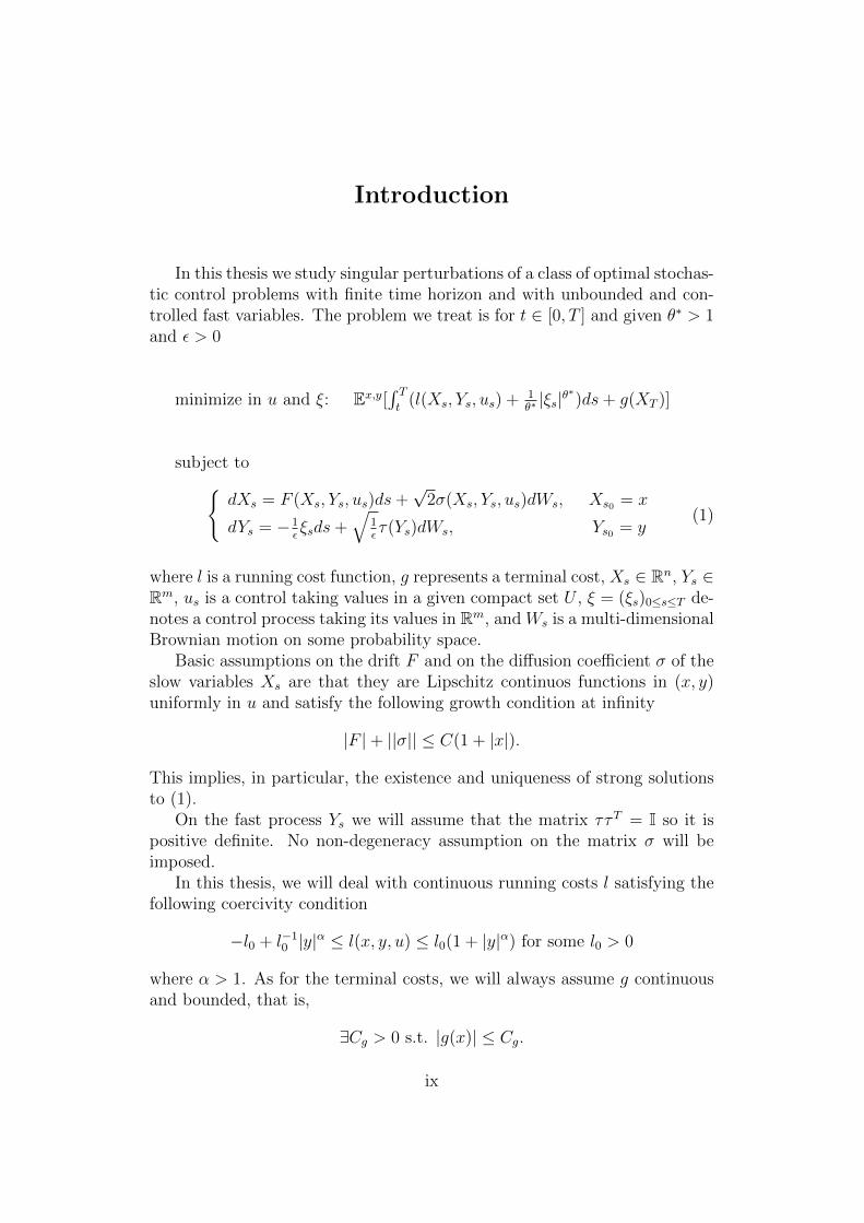
Introduction

In this thesis we study singular perturbations of a class of optimal stochas-tic control problems with finite time horizon and with unbounded and con-trolled fast variables. The problem we treat is for t ∈ [0, T ] and given θ∗ > 1and ε > 0

minimize in u and ξ: Ex,y[∫ Tt

(l(Xs, Ys, us) + 1θ∗|ξs|θ

∗)ds+ g(XT )]

subject todXs = F (Xs, Ys, us)ds+

√2σ(Xs, Ys, us)dWs, Xs0 = x

dYs = −1εξsds+

√1ετ(Ys)dWs, Ys0 = y

(1)

where l is a running cost function, g represents a terminal cost, Xs ∈ Rn, Ys ∈Rm, us is a control taking values in a given compact set U , ξ = (ξs)0≤s≤T de-notes a control process taking its values in Rm, and Ws is a multi-dimensionalBrownian motion on some probability space.

Basic assumptions on the drift F and on the diffusion coefficient σ of theslow variables Xs are that they are Lipschitz continuos functions in (x, y)uniformly in u and satisfy the following growth condition at infinity

|F |+ ||σ|| ≤ C(1 + |x|).

This implies, in particular, the existence and uniqueness of strong solutionsto (1).

On the fast process Ys we will assume that the matrix ττT = I so it ispositive definite. No non-degeneracy assumption on the matrix σ will beimposed.

In this thesis, we will deal with continuous running costs l satisfying thefollowing coercivity condition

−l0 + l−10 |y|α ≤ l(x, y, u) ≤ l0(1 + |y|α) for some l0 > 0

where α > 1. As for the terminal costs, we will always assume g continuousand bounded, that is,

∃Cg > 0 s.t. |g(x)| ≤ Cg.

ix

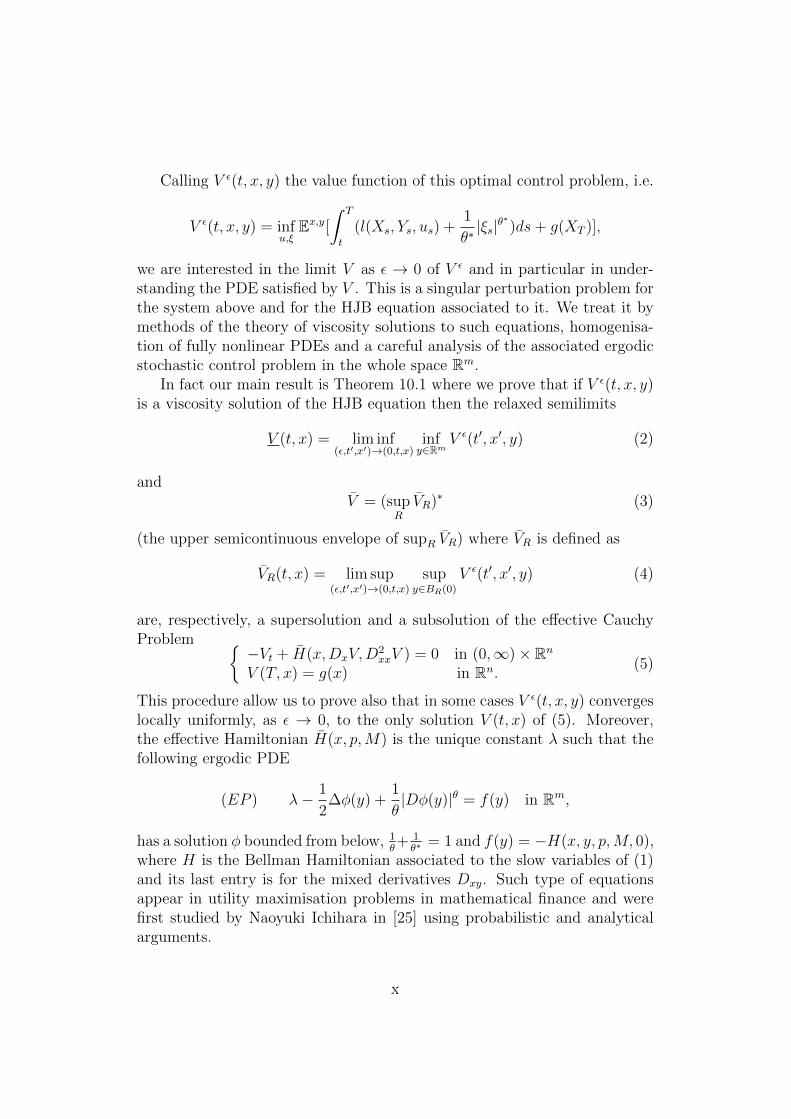
Calling V ε(t, x, y) the value function of this optimal control problem, i.e.

V ε(t, x, y) = infu,ξ

Ex,y[∫ T

t

(l(Xs, Ys, us) +1

θ∗|ξs|θ

∗)ds+ g(XT )],

we are interested in the limit V as ε → 0 of V ε and in particular in under-standing the PDE satisfied by V . This is a singular perturbation problem forthe system above and for the HJB equation associated to it. We treat it bymethods of the theory of viscosity solutions to such equations, homogenisa-tion of fully nonlinear PDEs and a careful analysis of the associated ergodicstochastic control problem in the whole space Rm.

In fact our main result is Theorem 10.1 where we prove that if V ε(t, x, y)is a viscosity solution of the HJB equation then the relaxed semilimits

V (t, x) = lim inf(ε,t′,x′)→(0,t,x)

infy∈Rm

V ε(t′, x′, y) (2)

andV = (sup

RVR)∗ (3)

(the upper semicontinuous envelope of supR VR) where VR is defined as

VR(t, x) = lim sup(ε,t′,x′)→(0,t,x)

supy∈BR(0)

V ε(t′, x′, y) (4)

are, respectively, a supersolution and a subsolution of the effective CauchyProblem

−Vt + H(x,DxV,D2xxV ) = 0 in (0,∞)× Rn

V (T, x) = g(x) in Rn.(5)

This procedure allow us to prove also that in some cases V ε(t, x, y) convergeslocally uniformly, as ε → 0, to the only solution V (t, x) of (5). Moreover,the effective Hamiltonian H(x, p,M) is the unique constant λ such that thefollowing ergodic PDE

(EP ) λ− 1

2∆φ(y) +

1

θ|Dφ(y)|θ = f(y) in Rm,

has a solution φ bounded from below, 1θ+ 1θ∗

= 1 and f(y) = −H(x, y, p,M, 0),where H is the Bellman Hamiltonian associated to the slow variables of (1)and its last entry is for the mixed derivatives Dxy. Such type of equationsappear in utility maximisation problems in mathematical finance and werefirst studied by Naoyuki Ichihara in [25] using probabilistic and analyticalarguments.

x

The main difficulty of (EP ) lies in the unbounded nature of our problem:first, the control region of ξ is not compact (all Rm), and consequently therunning cost |ξ|θ∗ is unbounded; second, f inherits the coercive growth of land tends to infinity at infinity; and, third, the superlinear nonlinearity inthe gradient implies that |Dφ(y)| → +∞ as |y| → ∞, in contrast with [37] or[21] where the gradient remains bounded on the whole space. Of course, thisunboundedness for the gradient complicates even more the arguments and toprove the solvability of (EP ) one needs to know more about the problem orthe equation itself. In fact, in our case, due to the form of equation (EP ),and the properties on f , we can use the results on the existence of solutionsand a priori bounds for second order quasilinear equations to guarantee theexistence of classical solutions of (EP ) (see Section 1). But if for the existencepart the methods used in [25] are analytical, for the study of the uniquenessIchihara’s methods are probabilistic. First, it is showed in [24] that thereexists a continuum of λ such that (EP ) has a solution. In fact, Ichiharashowed that there exists a critical value λ∗ such that for any λ < λ∗ (EP ) hasa solution (see also our Proposition 1.5). And so no uniqueness is expectedfor a general φ but at most for φ restricted to some classes. Second, givenany solution (λ, φ) of (EP ) we can define the diffusion process driven by

dY (s) = −Dqh(Dφ(Y (s)))dt+ dW (s), s ≥ 0, (6)

where Dqh(q) denotes the gradient of h(q) := 1θ|q|θ. Notice that such solu-

tion corresponds to the diffusion process obtained from (1) by taking ε = 1,and τ = I (that we will call for simplicity fast subsystem) and consider-ing ξ = Dqh(Dφ(Y (s))) the optimal control feedback (see Proposition 4.10of [25]). It can be shown that equation (EP ) and diffusion (6) are closelyrelated to a stochastic control problem with ergodic type criterion (which jus-tifies the name of ergodic stochastic control problem for the study of (EP )).Indeed, let ξ = (ξ(t))t≥0 be an Rm-valued control process belonging to someappropriate admissible class, say A, and let Y ξ = (Y ξ(t))t≥0 denote the as-sociated controlled process driven by

Y ξ(s) = y −∫ s

0

ξ(τ)dτ + W (s), s ≥ 0.

We consider the stochastic control problem of minimising the long-run aver-age cost

J(u, ξ) = lim infT→∞

1

TEx,y[

∫ T

0

(l(Xu,ξs , Y ξ

s , us) +1

θ∗|ξs|θ

∗)ds+ g(Xu,ξ

T )].

Then, under some suitable conditions, one can expect that

λ∗ = infu∈U ,ξ∈A

J(u, ξ),

xi

where λ∗ is the critical constant for the ergodic PDE (1), and that the feed-back control ξ∗(t) := Dqh(Dφ(Y (t))) with Y (t) defined by (6) gives theoptimal control. That is, only λ∗ allows us to define an optimal controlξ∗ for which Ys has good long-time behaviour (ergodicity). Thus studyingthe ergodicity of diffusion (6) plays a crucial role in solving rigorously thisminimization problem. It is proved in [25] that when Y ξ∗ is ergodic thereexists an invariant probability measure µ for Y ξ∗ and one can then prove that(EP ) has a unique solution pair (λ, φ) such that φ is bounded from belowand necessarily λ = λ∗.

In this thesis we prove again the uniqueness of (EP ) using new and purelyanalytical proofs. Indeed, if θ ≥ 2 we use the transformation z = −e−φ as thekey ingredient to prove uniqueness for solutions of (EP ) that are boundedfrom below (see section 4). In fact, such transformation allows us to showa comparison result for solutions of (EP ) in the complement of a large balland satisfying an apropriate Dirichlet condition. Then we argue by meansof the strong maximum principle inside the ball. We mention that with suchtransformation z we don’t need any type of knowledge about the behaviourof the solutions of (EP ) (other than the gradient bound that is necessary forthe existence). A different phenomenon occurs when θ < 2. In this case theuseful transformation is z = φq plus an estimate of the behaviour at infinityof solutions of (EP) bounded from below: they necessarily grow with somespecific power that will appear many times in this thesis. All this and moreis explained and showed in Section 4.

Properly equipped with these new tools we are able to build up all theresults on the ergodic Bellman equation that we need and we can also provesome procedures that are useful for Chapter 2. In this sense, this thesis isself contained. With our new proofs it is easy to see that, if (λ, φ) is a pairsolution of (EP ) such that φ is bounded from below, then necessarily wehave λ = λ∗ (Section 5). This is the result that we mentioned earlier forthe ergodic diffusion Y ξ∗ but now we don’t need anymore to argue with theergodic measure. Also, with the new proofs, we can show new non-standardapproximation results for (EP ) that are extremely useful in the proof of theconvergence theorem of Section 10 when we introduce the perturbed testfunction method. In Section 6, we first treat approximations of (EP ) byperturbing f with truncations of f . And then we consider approximationsof (EP ) by looking at the ergodic PDE defined on the ball BR(0) and com-plemented with a boundary condition that reads differently according to thevalue of θ. In fact, we look at

λR − 12∆φR(y) + 1

θ|DφR(y)|θ = f(y) in BR(0)

φR(y)→ +∞ as y → ∂BR(0)

xii

for 1 < θ ≤ 2

and λR − 1

2∆φR(y) + 1

θ|DφR(y)|θ = f(y) in BR(0)

λR − 12∆φR(y) + 1

θ|DφR(y)|θ ≥ f(y) on ∂BR(0)

for θ > 2.The key features of such approximations are that, first, considering per-

turbations of f , we can control the growth of the corrector in the perturbedtest function method as we wish and, second, considering approximationsof (EP ) by balls, we consider only correctors that “explode” on the bound-ary of BR(0). This is important because it forces the maximum point to beachieved only inside BR(0), as it will be explored in Section 6, and this is acrucial element for Section 10. For more details we refer the reader to Section6. Here, we wish to stress that our main motivation in Section 6 is indeedthe proof of Theorem 10.1.

We prove a convergence theorem for the singular perturbation problemof our stochastic model with controlled and unbounded fast variables byusing non-standard relaxed semilimits and we give some examples that testour result. We are now in conditions to discuss the Convergence Theorem,Theorem 10.1, the main result of this thesis. First we notice that λ∗ isthe appropriate constant to define the effective Hamiltonian H appearing inthe Cauchy effective problem. Second, due to the unbounded nature of ourproblem and the fact that we wish to define the relaxed semilimits in a waythat gets rid of y, the standard relaxed semilimits

V (t, x, y) = lim inf(ε,t′,x′,y′)→(0,t,x,y)

V ε(t′, x′, y′)

andV (t′, x′, y′) = lim sup

(ε,t′,x′,y′)→(0,t,x,y)

V ε(t′, x′, y′)

cannot be applied successfully. This is a difficulty that we overcome byintroducing new relaxed semilimits V and V as in (2) and (3). The lowerrelaxed semilimit is similar to the one used in periodic singular perturbations,but something different must be done for V . The main difference is thatwe can control how V ε grows from below but not completely from above.The upper relaxed semilimit V gives us more troubles but it is also themost interesting to treat. With all the machinery introduced in the earliersections we can prove that (2) and (3) are respectively a supersolution and asubsolution of the Cauchy effective problem. In the corollaries and exampleswe test our convergence theorem.

xiii

We finish this Introduction with some historical remarks on the theme.Singular perturbations of diffusion processes, with and without controls, havebeen studied by many authors. For results based on probabilistic methodswe refer to the books [27, 29], papers [34, 13], and the references therein. Foran approach based on PDE-viscosity methods for the HJB equations we referthe worked developed by Alvarez and Bardi in [1, 2, 3], also [4] for problemswith an arbitrary number of scales. It allows to identify the appropriatelimit PDE governed by the effective Hamiltonian and gives general conver-gence theorems of the value function of the singularly perturbed system tothe solution of the effective PDE, under assumptions that include determin-istic control as well as differential games, in deterministic and stochasticcases. However, this theory originating in periodic homogenisation problems(in papers [33, 19]) was developed mostly for fast variables restricted to acompact set, almost all in the case of the m-dimensional torus. Nonethelessin many financial models the a priori knowledge of the boundedness of thefast variables does not appear to be natural according to the empirical data.

In the papers [7] and [6] the authors present an extension of the meth-ods based on viscosity solutions showed in [1, 2, 3] to singular perturbationproblems that have unbounded but uncontrolled fast variables.

This thesis is divided in two chapters. In Chapter I we study (EP ) andin Chapter II we study our singular perturbation problem.

Main results of this thesis:

• Chapter I: Study of (EP ) by purely PDE methods, introduction ofnon-standard approximations for (EP ) that will be useful in ChapterII.

• Chapter II: The convergence theorem, our main result. Our relaxedsemilimits are not typical and the proof of this convergence uses manyof the procedures introduced and developed in Chapter I. We presentsome cases where V ε really converges locally uniformly to V , solutionof the effective Cauchy problem, as ε → 0. It is, as far as we know,the first singular perturbation problem of a stochastic model with un-bounded and controlled fast variables that is treated with success. Wetreat everything analytically. We believe that some of our ideas can beapplied with success to the study of other singular perturbation models.

xiv

Chapter IThe Ergodic Problem

1

This Chapter is organised as follows. In Section 1 we study the solvabilityof (EP ) and we prove that it has infinitely many solutions and a critical value.Section 2 is devoted to the construction of solution bounded from below of(EP ). We prove that there exists a solution φ ∈ C2(Rm) such that thereexists R > 0 such that φ(y) ≥ C|y|β for all |y| ≥ R. These first two sectionsare connected to Ichihara work, namely, the papers [24] and [25].

Section 3 considers (EP ) defined in the ball and complemented witha state constraint boundary condition which is different according to thevalue of θ. We study such ergodic problems and we give some propertiesof the ergodic constant. This section is a preparation for the most generalapproximation results considered in Section 6. The main references in thissection are [31], [10], and [38].

Next sections are an original part.Section 4 deals with the problem of the uniqueness of the ergodic constant

and of the corrector (up to additive constants) of (EP ). This problem wasalso studied by Naoyuki Ichihara in [25] but our methods differ very muchfrom his probabilistic arguments. Here we present a full PDE proof.

Section 5 is concerned with some properties of the ergodic constant λ forsolutions of (EP ) that are bounded from below. We also give some estimatesthat will be useful in Section 10.

Sections 6 shows new convergence results for (EP ). There we considerapproximations of (EP ) by perturbing f or by specific ergodic problems seton balls. This section is mainly motivated by the problem studied in Chapter2 though it has interest in itself.

Appendices are devoted to review some well established results or topresent some technical computation or estimate needed in the text.

2

Part I

Existence

3

1 Solvability of (EP )

This part is concerned with the existence of solutions of (EP ). Our problemis to find a pair (λ, φ) ∈ R× C2(Rm) such that for given θ > 1

(EP ) λ− 1

2∆φ(y) +

1

θ|Dφ(y)|θ = f(y) in Rm.

Here Dφ and ∆φ denotes respectively the gradient and the Laplacian of φ.

Definition (Solution, Subsolution and Supersolution for (EP )) Wewill call a pair (λ, φ) a solution ( resp. subsolution, supersolution) of (EP )if λ ∈ R, φ : Rm −→ R belongs to C2(Rm), and

λ− 1

2∆φ(y) +

1

θ|Dφ(y)|θ = f(y) (resp. ≤ f(y), ≥ f(y))

for all y ∈ Rm.

Our assumption on f is

(H1) f ∈ W 1,∞loc (Rm) and there exists f0 > 0 and α > 0 such that

−f0 + f−10 |y|α ≤ f(y) ≤ f0|y|α + f0

and|Df(y)| ≤ f0(1 + |y|α−1)

for all y ∈ Rm.

Notice that this implies that ∀λ,M > 0 we can find R > 0 such thatf(y) − λ ≥ M for all |y| ≥ R. We will exploit condition (H1) in severaloccasions.

For simplicity of notation, let G be the operator

G[φ](y) := −1

2∆φ(y) +

1

θ|Dφ(y)|θ − f(y).

Then (EP ) is equivalent to

G[φ](y) = µ in Rm (7)

with µ = −λ.

Important remark: Since φ 7→ 1θ|Dψ|θ is strictly convex and Laplacian

is a linear operator, it is easy to see that G is a stricly convex operator. Thisconvexity will play a crucial role in the arguments.

4

Definition (Holder Spaces) For given k ∈ N∪0 , ι ∈ (0, 1] and an openset O ⊂ Rm, we define the Holder space Ck,ι(O) by

Ck,ι(O) := v ∈ Ck(O)| supx,y∈O,x6=y

|Dav(x)−Dav(y)||x− y|ι

<∞, |a| = k,

where a stands for a multi-index of Differential operator D. We denote byCk,ι(Rm) the set of all functions v ∈ Ck(Rm) such that v ∈ Ck,ι(O) for anybounded O.

Let I be the operator

I(y, q) :=1

θ|q|θ − f(y) (8)

hence we can write

G[φ](y) = −1

2∆φ(y) + I(y,Dφ(y)).

Remark: By virtue of (H1) we have that for all |y| ≤ R there exists aconstant CR > 0 such that |I(y, q)| ≤ CR(1 + |q|θ).

1.1 Functions φβ

We start by giving a very important class of functions.

Lemma 1.1 There are constants c0, ν0 and ρ0 ∈ (0, 1) such that for any

ρ ∈ (−ρ0, ρ0), φβ(y) := ρ(1 + |y|2)β2 , satisfies

G[φβ](y) ≤ −c0|y|α + ν0, y ∈ Rm (9)

where β ∈ [0, αθ

+ 1].

Proof This proof can be found in [25]. Let ρ ∈ (−1, 1). We have

Dφβ(y) = βρ(1 + |y|2)β−22 y,

and

∆φβ = βρ[m(1 + |y|2)β−22 + (β − 2)|y|2(1 + |y|2)

β−42 ]

= βρ[(β − 2)|y|2 +m(1 + |y|2)](1 + |y|2)β−42 .

5

Since β ≤ αθ

+ 1 ≤ α+ 2 implies θ(β− 1) ≤ α and β− 2 ≤ α, we see, in viewof our assumption on f , (H1), and |ρ| ≤ 1⇒ |ρ|θ ≤ |ρ| (θ > 1), that

G[φβ](y) = −1

2∆φβ(y) +

1

θ|Dφβ(y)|θ − f(y)

≤ C1(1 + |ρ||y|β−2 + |ρ|θ|y|θ(β−1)) + f0 − f−10 |y|α

≤ C2(1 + |ρ||y|α + |ρ||y|α) + f0 − f−10 |y|α

≤ (2|ρ|C2 − f−10 )|y|α + f0 + C2

for some constant C2 > 0 independent of ρ and that we can make it inde-pendent of β too (by taking larger C2 if necessary). Now choosing ρ0 ∈ (0, 1)so small such that ρ0 < (2C2)−1f−1

0 and defining c0 := f−10 − 2ρ0C2 > 0 and

ν0 := f0 + C2 we can conclude (9).

Observe that φβ given by Lemma 1.1 satisfies

lim|y|→∞

G[φβ](y) = −∞. (10)

Fix any φβ := ρ0(1 + |y|2)β2 in the conditions of Lemma 1.1. As we will see

next, such function φβ is enough to guarantee the existence of a solution for(EP ).

1.2 Existence of solutions for (EP )

The goal of this subsection is to show Theorem 1.2. We follow [24]. Theproof proceeds essentially in the same lines of [28, Section 2].

Let C∞c (Rm) be the set of infinitely differentiable functions on Rm withcompact support. For k ∈ N ∪ 0, p ∈ [1,∞] and an open set O ⊂ Rm, wedefine the Sobolev space W k,p(O) by the collection of all locally summablefunctions v on O such that for each multi-index a with |a| ≤ k, Dav existsin the weak sense and belongs to Lp(O). We denote by W k,p

loc (Rm) the setof locally summable functions v on Rm such that vζ ∈ W k,p(Rm) for allζ ∈ C∞c (Rm).

Before starting the proof of Theorem 1.2, we first remark that any weaksolution of (7) (and therefore (EP )) in the distribution sense belonging toW 1,∞

loc (Rm) is indeed a classical solution. This is a direct consequence of theclassical regularity theory for quasilinear elliptic equations. Furthermore, inview of the Schauder theory, any classical solution of (7) ((EP )) is a C3-solution (see [23]).

6

Theorem 1.2 There exists a constant µ0 such that (7) has a solution withµ = µ0.

Proof This proof can be found in [24, Proposition 3.2]. Since we have (10)then we know that there exists µ0 ∈ R such that G[φβ](y) < µ0 ∀y. Thistogether with Theorem B.1(b) implies that for any R > 1, there exists asolution φR ∈ C2,ι(BR) of

G[φR] = µ0 in BR, φR = φβ on ∂BR.

By Corollary B.2, we have that |DφR| is uniformly bounded by a constant notdepending on R. Then, using the classical regularity theory for quasilinearelliptic equations (see [23]), we have that the Holder norm |DφR|Γ,BR for someΓ ∈ (0, 1) is bounded by a constant not depending on R. By Schauder’s the-ory for linear elliptic equations, we also have that the Holder norm |φR|Γ,BRis bounded by a constant not depending on R. In particular, the familyφRR>1 is relatively compact. By Arzela-Ascoli Theorem, we can concludethat there exist a sequence Rnn diverging to infinity as n→∞ such thatφnn := φRnn converges to a function φ ∈ C0,1

loc (Rm) = W 1,∞loc (Rm) locally

uniformly in Rm. Next, we prove that φ is is a weak solution of G[φ] = µ0 inRm in the distribution sense.

Indeed, fix any ζ ∈ C∞c (Rm) and some R > 1 such that supp ζ ⊂ BR.Observe that for any n, we have by integration,

1

2

∫BR

Dφn(y) ·Dζ(y)dy +

∫BR

I(y,Dφn(y))ζ(y)dy = µ0

∫BR

ζ(y)dy. (11)

where I was introduced in (8). Since supn |Dφn|L∞(BR) < ∞, we see that

φn − φ → 0 weakly in W 1,2loc (Rm). Moreover, we can verify that φn − φ → 0

strongly in W 1,2loc (Rm) as n→∞. Indeed, replacing ζ in (11) by the function

(φn − φ)ζ, we first see that

1

2

∫BR

Dφn · (Dφn −Dφ)ζdy = −1

2

∫BR

Dφn · (φn − φ)Dζdy

−∫BR

I(y,Dφn)(φn − φ)ζdy + µ0

∫BR

(φn − φ)ζdy

and then we take into account the equality Dφn(y) = (Dφn(y) − Dφ(y)) +

7

Dφ(y) and the bound |I(y, q)| ≤ CR(1 + |q|θ) for all |y| ≤ R to conclude that∫BR

|Dφn(y)−Dφ(y)|2ζ(y)dy

≤ −∫BR

(Dφn(y)−Dφ(y))ζ(y)Dφ(y)dy

+

∫BR

|Dφn(y)||φn(y)− φ(y)||Dζ(y)|dy

+ 2CR

∫BR

(1 + |Dφn(y)|θ)|φn(y)− φ(y)||ζ(y)|dy

+ 2µ0

∫BR

(φn(y)− φ(y))ζ(y)dy.

Since the right-hand side converges to zero as n→∞, we obtain the strongconvergence φn − φ→ 0 in W 1,2

loc (Rm). Thus, letting n→∞ in (11), we get

1

2

∫Rm

Dφ(y) ·Dζ(y)dy +

∫Rm

I(y,Dφ(y))ζ(y)dy = µ0

∫Rm

ζ(y)dy

for all ζ ∈ C∞c (Rm). Hence, φ is a weak solution of G[φ] = µ0 in Rm inthe distribution sense. By the standard regularity arguments for quasilinearelliptic equations, we conclude that φ is indeed a C2-solution (in fact, C3-solution).

Corollary 1.3 (EP ) has a solution.

Important Remark: For the solvability of (EP ) the only information thatis used is the existence of a function φβ satisfying (10). Therefore the proofworks for any other solution satisfying the same condition. We can state

Proposition 1.4 If there exist φ ∈ C3(Rm) such that lim|y|→∞G[φ](y) =−∞ then (EP ) has a solution.

1.3 Infinite number of solutions

Proposition 1.5 If (λ1, φ) is a sub solution of (EP ), then there exist asolution of (EP ) for any λ2 < λ1.

Proof Let (λ1, φ) be a sub solution of (EP ). Then, G[φ] ≤ −λ1 < −λ2. ByTheorem B.1(b) (Appendix B), we know that for any R > 1 there exists asolution φR ∈ C2,ι(Rm) of

G[φR] = −λ2 in BR, φR = ψ on ∂BR.

Consider the family φRR>1. The conclusion follows by applying the sameargument as in in Theorem 1.2.

8

Remark: Theorem 1.2 and Proposition 1.5 shows that there are infinitelymany solutions of (EP ).

1.4 Existence of a critical value

Proposition 1.6 Set λ∗ := supλ ∈ R| (EP ) has a subsolution. Then λ∗

is finite and there exists a solution associated to it.

Proof Theorem 1.2 implies λ∗ 6= −∞ because λ∗ ≥ −µ0 with µ0 ∈ R. Toprove that λ∗ < +∞, suppose, by contradiction, that λ∗ = +∞. Then, thereexists a sequence of subsolutions (λk, φk)k of (EP ) such that limk→∞ λk =+∞. Fix any ζ ∈ C∞c (Rm). We have, by integration by parts,

1

2

∫Rm

Dφk(y)Dζ(y)dy +

∫Rm

(1

θ|Dφ(y)|θ − f(y)

)ζ(y)dy ≤ −λk

∫Rm

ζ(y)dy

for all k. By Corollary B.3 (gradient bound), we know that the left-hand sideis bounded uniformly in k. Therefore, taking k → ∞ yields a contradictionbecause the right-hand side of the above equality goes to −∞ as k → ∞.Therefore λ∗ is finite.

We can now choose any (λk, φk)k such that G[φk] = −λk := µk in Rm

for each k and limk→∞ λk = λ∗. Then, it is an obvious consequence of thegradient bound and the argument in Theorem 1.2, that φk converges to afunction φ that is indeed a C2-solution of (EP ) with λ = λ∗.

Notation: Sometimes we will refer to λ∗ as λ∗(f) to stress the dependenceof (EP ) on f .

Corollary 1.7 There exists a constant λ∗ ∈ R such that (EP ) admits aclassical solution φ ∈ C2(Rm) if and only if λ ≤ λ∗.

By combining Propositions 1.5 and 1.6 we get the following conclusion.

Proposition 1.8 (Monotonicity of λ∗ with respect to f) Suppose that f1, f2

satisfy (H1). If f1 ≤ f2, then λ∗(f1) ≤ λ∗(f2).

Proof By Proposition 1.6 we know that there exists a solution φ1 associatedto λ∗(f1) and a solution φ2 associated to λ∗(f2). If f1 ≤ f2 then (λ∗(f1), φ1)is a subsolution of (EP ) with f = f2. By definition of λ∗(f2), we have thatλ∗(f1) ≤ λ∗(f2).

Remark: Observe that this result is true for any f1, f2 satisfying (H1) pos-sibly with different constants and exponents.

9

Proposition 1.9 Assume that f satisfies assumption (H1). Then

λ∗(f + c) = λ∗(f) + c where c ∈ R.

Proof Let (λ∗(f), φ1) be a solution of (EP ) given by Proposition 1.6 andlet (λ∗(f + c), φ2) be a solution of (EP ) with f = f + c given by Proposition1.6.

We have

(λ∗(f) + c)− 1

2∆φ1 +

1

θ|Dφ1|θ = f + c

Consequently, by definition of λ∗(f + c),

λ∗(f) + c ≤ λ∗(f + c). (12)

On the other hand,

(λ∗(f + c)− c)− 1

2∆φ2 +

1

θ|Dφ2|θ = (f + c)− c = f

and we can see thatλ∗(f + c) ≤ λ∗(f) + c. (13)

Therefore using (12) and (13), we have that λ∗(f + c) = λ∗(f) + c as wewished to show.

Proposition 1.10

λ∗(c|y|α) = cθ∗

θ∗+αλ∗(|y|α).

Proof Let (λ∗(|y|α), φ1) be a solution of (EP ) with f(y) = |y|α given byCorollary 1.7. We will now construct a solution of (EP ) with f(y) = c|y|α

by considering φ2(y) = β2−θθ−1φ1(βy) and the right choice of β.

We have,

−1

2∆φ2(y) +

1

θ|Dφ2(y)|θ = −1

2∆(β

2−θθ−1φ1(βy)) +

1

θ|D(β

2−θθ−1φ1(βy))|θ

= −1

2β

θθ−1 ∆(φ1(βy)) +

1

θβ

θθ−1 |Dφ1(βy)|θ

= βθθ−1

(− 1

2∆(φ1(βy)) +

1

θ|Dφ1(βy)|θ

)= βθ

∗(βα|y|α − λ∗(|yα|)

)

10

using the chain rule for the second equality and the fact that (λ∗(|y|α), φ1)is a solution of (EP ) with f(y) = |y|α and θ

θ−1= θ∗ for the last.

Therefore

βθ∗λ∗(|yα|)− 1

2∆φ2(y) +

1

θ|Dφ2(y)|θ = βθ

∗+α|y|α

and choosing βθ∗+α = c, i.e., β = c

1θ∗+α we arrive at

cθ∗

θ∗+αλ∗(|yα|)− 1

2∆φ2(y) +

1

θ|Dφ2(y)|θ = c|y|α

By definition of λ∗(c|y|α), we obtain

cθ∗

θ∗+αλ∗(|yα|) ≤ λ∗(c|y|α).

The reverse inequality is obtained in an equivalent manner by looking atthe solution (λ∗(c|y|α), ψ1) of (EP ) with f(y) = c|y|α given by Corollary 1.7and then construction a solution of (EP ) with f(y) = |y|α by considering

ψ2(y) = β2−θθ−1ψ1(βy) and β = (1

c)

1θ∗+α .

Conclusion: λ∗(c|y|α) = cθ∗

θ∗+αλ∗(|yα|).

11

2 Bounded from below solutions of (EP )

Theorem 1.2 shows that (EP ) has a solution for any φβ = ρ0(1 + |y|2)β2

in the conditions of Lemma 1.1. In this section, our goal is to construct asuitable solution by an analytical approximation procedure (approximationby Dirichlet problems) satisfying a certain growth from below. In fact, wewill build a solution (λ, φ) ∈ R × C2(Rm) of (EP ) such that infRm(φ − φβ)is finite.

2.1 Estimate for solutions of (EP )

Proposition 2.1 Let (λ, φ) be a solution of (EP). Then there exists a K > 0such that

|Dφ(y)| ≤ K(1 + |y|γ−1), |φ(y)| ≤ K(1 + |y|γ), y ∈ Rm,

where γ = αθ

+ 1.

Proof From Corollary B.3 in Appendix B, we have for all r > 0 that thereexists a constant C > 0 such that

supBr

|Dφ(y)| ≤ C(1 + supBr+1

|f(y)− λ|1θ + sup

Br+1

|Df(y)|1

2θ−1 ).

Using now hypothesis (H1), we see that

supBr

|Dφ| ≤ C(1 + (r + 1)αθ + (r + 1)

α−12θ−1 ).

for another C > 0. Since αθ

= γ − 1 and α−12θ−1

< γ − 1, we can conclude that

supBr

|Dφ| ≤ C + C(r + 1)γ−1

with C > 0. From this inequality we can deduce the first estimate of thisproposition. The second one is deduced by integration from the first one.Hence, we have completed the proof.

An heuristic justification: In fact, from the type of growth assumed onf , we would expect φ(y) to have a polynomial growth on y. Now assume forsimplicity that φ(y) = |y|β for some power β > 0 and that we are “away”from y = 0. Then Dφ is of order |y|β−1 while ∆φ is of order |y|β−2. Since f(y)

12

growths like |y|α at infinity (see (H1)) we have, plugging into the equationλ− 1

2∆φ(y) + 1

θ|Dφ(y)|θ = f(y), that

O(|y|β−2 + |y|θ(β−1)) ≤ O(|y|α)

(which translates the fact that the left-hand side cannot exceed in growththe right-hand side). But β − 2 < β − 1 < θ(β − 1) (because θ > 1) henceO(|y|β−2 + |y|θ(β−1)) = O(|y|θ(β−1)) (here we use the fact that y is not closeto 0!), and obviously θ(β− 1) ≤ α =⇒ β ≤ α

θ+ 1 := γ. Hence the maximum

growth expected is of order γ!Notice that, if y is “close to 0”, the quantities |y|β−2, |y|θ(β−1) may ex-

plode according to the values of β. The reason why we considered φ0 above,is because φ0 behaves like a polynomial of order β at infinity but is twicedifferentiable in all Rm.

The exponent γ: From now on, γ will denote the value γ := αθ

+ 1 .

2.2 The class Φβ

We will denote by Cp(Rm) the set of continuous functions on Rm that havepolynomial growth, that is,

Cp(Rm) = v ∈ C(Rm) : ∃q, C > 0 s.t. |v(y)| ≤ C(1 + |y|q).

As Proposition 2.1 shows if (λ, φ) is a solution of (EP ) then φ ∈ Cp(Rm).

For given β ∈ [0, γ], consider

Φβ := v ∈ C2(Rm) ∩ Cp(Rm)| lim inf|y|→∞

v(y)

|y|β> 0.

Our aim is to construct a solution of (EP ) belonging to Φβ.

2.3 Existence of a solution of (EP ) in Φβ

For any ε ∈ (0, 1) and β ∈ [0, γ], let us consider the elliptic equation

G[φ] + εφ = εφβ in Rm (14)

for any φβ := ρ0(1 + |y|2)β2 satisfying Lemma 1.1 for some ρ0 ∈ (0, 1).

13

Lemma 2.2 (Similar to Lemma 1.1) There is a constant ρ1 > 1 such thatψγ(y) := ρ1(1 + |y|2)

γ2 , satisfies

G[ψγ](y) ≥ −K in Rm

for some K > 0.

Proof The proof is similar to Lemma 1.1’s proof. We have, in view of (H1)and the computations presented in Lemma 1.1 with β = γ, that

G[ψγ] ≥ −ρ1C1(1 + |y|γ−2) + C2|ρ1|θ|y|θ(γ−1) − f0(1 + |y|α)

for some constants C1 and C2 positive that do not depend on the value of ρ1

and γ. Since θ(γ − 1) = α and γ − 2 ≤ α, we can see that

G[ψγ] ≥ (−ρ1C1 + C2|ρ1|θ − f0)|y|α − f0 − ρ1C1

If we choose ρ1 large enough such that −ρ1C1 + C2|ρ1|θ − f0 ≥ 0 and takeK := f0 + ρ1C1 the conclusion follows.

Proposition 2.3 For any sufficiently small ε > 0, there exists a solutionvε ∈ C2(Rm) of (14) such that infRm(vε − φβ) is finite. Moreover, we havethat εvε(0) is bounded by a constant that does not depend on ε.

Proof The proof is divided into three parts. Fix an arbitrary ε > 0 andconsider the ψγ of Lemma 2.2. Because 0 < ρ0 < 1 < ρ1 and β ≤ γ, we have

that φβ = ρ0(1 + |y|2)β2 ≤ ρ1(1 + |y|2)

γ2 = ψγ in the whole space Rm.

Let ν0 be the constant in Lemma 1.1.

Step 1. φβ − ν0ε

and ψγ + Kε

are respectively a subsolution and a super-solution of (14)

We have,

G[φβ −

ν0

ε

]+ ε(φβ −

ν0

ε

)= G[φβ] + εφβ − ν0 ≤ −c0|y|α + εφβ ≤ εφβ.

Where we use (9) in the first inequality. Therefore φβ − ν0ε

is a subsolutionof (14).

Analogously, one can see that

G[ψγ +

K

ε

]+ ε(ψγ +

K

ε

)= G[ψγ] + εψγ +K ≥ εψγ ≥ εφβ,

14

and conclude that ψγ + Kε

is a supersolution of (14). Observe that here weuse Lemma 3.2 in the first inequality and φβ ≤ ψγ in Rm in the last one.

Step 2. There exist a C2-solution vε of (8) such that

φβ(y)− ν0

ε≤ vε(y) ≤ ψγ(y) +

K

εin Rm.

Fix any R > 0 and consider the Dirichlet problem

G[vε,R] + εvε,R = εφβ in BR, vε,R = φβ on ∂BR.

By virtue of Theorem B.1(a) in Appendix B, for any R > 1 there exists asolution in the class vε,R ∈ C2,ι(BR). Moreover, since φβ − ν0

εand ψγ + K

ε

are, respectively, sub- and supersolutions of (14) that satisfy φβ − ν0ε≤

vε,R = φβ ≤ ψγ + Kε

on ∂BR, a standard comparison principle implies thatφβ − ν0

ε≤ vε,R ≤ ψγ + K

εin BR. Furthermore, by Theorem B.2, we have

that supBr |Dvε,R| ≤ C where the constant C does not depend on R and ε.Thus, by the Ascoli-Arzela theorem and the same argument as in the proofof Theorem 1.2, there exists a weak solution vε ∈ W 1,∞

loc (Rm) of (14) in thedistribution sense, which is indeed of C2-class by the standard regularity ar-guments.

Step 3. infRm(vε − φβ) is finite and εvε(0) is bounded by a constant thatdoes not depend on ε.

Since vε satisfies

φβ(y)− ν0

ε≤ vε(y) ≤ ψγ(y) +

K

εin Rm,

we have that infRm(vε − φβ) ≥ −ν0ε

. Multiplying now the above inequalityby ε, we get

εφβ(0)− ν0 ≤ εvε(0) ≤ εψγ(0) +K in Rm.

Hence, ε|vε(0)| ≤ C for all ε ∈ (0, ε0) for some ε0. Thus εvε(0) is bounded bya constant that does not depend on ε.

Theorem 2.4 There exists a solution (λ, φ) of (EP ) such that infRm(φ−φβ)is finite.

Proof Let vε be the solution given by Proposition 2.3 and define wε(y) :=vε(y)− vε(0) and λε := εvε(0). It is obvious that (λε, wε) is a solution of

λε +G[wε] + εwε = εφβ in Rm, wε(0) = 0.

15

By Theorem B.2 in Appendix B, we observe that, for any R > 0, supBR |Dwε|is bounded by a constant not depending on ε. In particular, repeating theargument of Theorem 1.2, we can prove that the family wεε>0 is relativelycompact in C(Rm). By the Ascoli-Arzela theorem, there exist a sequenceεkk → 0 as k → ∞, a function φ ∈ W 1,∞

loc (Rm) and a constant λ suchthat εkvεk(0) → λ and wεk → φ in C(Rm) as k → ∞. As in the proof ofTheorem 1.2, φ is a solution of G[φ] = −λ := µ in Rm in the distributionsense and therefore, by the standard regularity arguments, φ is a C2-solutionof G[φ] = µ in Rm, that is, (λ, φ) is a solution of (EP ).

We show next that infRm(φ − φβ) is finite. For that, notice first that, byconvexity of G, Lemma 1.1 and (H1), we have for any δ ∈ (1/2, 1) andy ∈ Rm

G[δφβ](y) = G[δφβ + (1− δ)0](y)

≤ δG[φβ](y) + (1− δ)G[0](y)

≤ −δc0|y|α + δν0 + (1− δ)(−f(y))

≤ −1

2c0|y|α + ν0 + (1− δ)f−1

0 − (1− δ)f0|y|α

≤ −1

2c0|y|α + ν0 +

1

2f0−1.

Taking into account this last estimate and Proposition 2.3, we can chooseR > 0 so big such that

G[δφβ](y) ≤ −C1 ≤ εvε(0) for all |y| ≥ R, ε ∈ (0, ε0) and δ ∈ (1/2, 1) (15)

and then find an MR > 0 such that sup0<ε<ε0 supy∈BR(|φβ| + |wε|) ≤ MR.Observe that MR is finite because supBR |wε| is bounded by a constant notdepending on ε.

We will now prove that wεk satisfies wεk ≥ δφβ −MR in Rm for all δ ∈(1/2, 1). To see this, we will argue in different regions of space. First, wehave that

wεk(y)− δφβ(y) ≥ − supBR

(|φβ|+ |wεk |)) = −MR for all |y| ≤ R. (16)

Hence, the claim is true in BR. From another point of view, since

wεk(y)− δφβ(y) +MR = (wεk − φβ)(y) + (1− δ)φβ(y) +MR → +∞ (17)

as |y| → +∞ (recall that infRm(wεk − φβ) is finite by Proposition 3.3), theclaim also holds for a Rεk,δ > R such that

wεk(y) ≥ δφβ(y)−MR for all |y| ≥ Rεk,δ.

16

Hence, the claim is also true in BcRεk,δ

.

It remains to show that it is also verified in the ring D := y ∈ Rm|R <|y| < Rεk,δ. For that, we will show that δφβ −MR and wεk are respectivelya sub and a supersolution of

G[v] + εkv = εkφβ − C1 in D,

(C1 is the constant in (15)) and then conclude by means of the comparisontheorem that δφβ −MR ≤ wεk in D.

For any y ∈ D, we have, using (15) and the fact that MR > 0,

G[δφβ −MR](y) + εk(δφβ(y)−MR) = G[δφβ](y) + εk(δφβ(y)−MR)

≤ −C1 + εk(φβ(y)−MR)

≤ εkφβ(y)− C1

and

G[wεk ](y) + εkwεk(y) ≥ εkφβ(y)− λεk= εkφβ(y)− εkvεk(0)

≥ εkφβ(y)− C1.

Therefore, δφβ −MR and wεk are respectively a subsolution and a superso-lution of

G[v] + εkv = εkφβ − C1 in D,

that satisfy δφβ − MR ≤ wεk on ∂D (look at (16) when |y| = R and at(17) when |y| = Rεk) . Applying a standard comparison principle, we obtainδφβ −MR ≤ wεk in D. Therefore, the claim also holds in D.

Consequently, δφβ −MR ≤ wεk in Rm for all δ ∈ (1/2, 1). Letting δ → 1, weconclude that φβ −MR ≤ wεk in Rm. Taking k →∞ we get infRm(φ−φβ) ≥−MR as we would like to prove.

Remark: Observe that the convexity of G plays a crucial role in this proof.

It is obvious that if infRm(φ−φβ) is finite then lim inf |y|→∞φ(y)|y|β > 0. Therefore

Corollary 2.5 There exists a solution (λ, φ) of (EP ) such that φ belongs to

Φβ := v ∈ C2(Rm) ∩ Cp(Rm)| lim inf|y|→∞

v(y)

|y|β> 0.

17

In particular, if we take β = γ := αθ

+ 1, we can conclude that

Corollary 2.6 There exists a solution (λ, φ) of (EP ) such that φ belongs to

Φγ := v ∈ C2(Rm) ∩ Cp(Rm)| lim inf|y|→∞

v(y)

|y|γ> 0.

We ask the reader to keep in mind this class Φγ.

Observation: Φγ ⊆ Φβ ⊆ bounded from below.

18

3 Approximations

Let θ > 1 and consider the ergodic problem in BR(0) (R > 0),

λR −1

2∆φR(y) +

1

θ|DφR(y)|θ = fR(y) in BR(0) (18)

complemented with a state constraint boundary condition which is differentin the sub and superquadratic case.

We start with some local gradient bounds for solutions of (18) plus theboundary condition.

Theorem 3.1 (Local Gradient Bound) Assume that for any fixed λR thereexist a solution φR ∈ W 2,p

loc (BR(0)) (p < +∞) of (18) satisfying the boundarycondition. Then, if fR ∈ W 1,∞(BR(0)), we have for all 0 < R′ < R

|DφR(y)| ≤ CR′ if y ∈ BR′(0)

where CR′ depends only on bound on DfR, upper bounds on fR − λR and θ.

Proof This proof can be found in [31, in Appendix].

3.1 Subquadratic and quadratic cases

For any R > 0 considerλR − 1

2∆φR(y) + 1

θ|DφR(y)|θ = fR(y) in BR(0)

φR(y)→ +∞ as y → ∂BR(0).(19)

Theorem 3.2 (Existence and uniqueness of solutions for (19)) Assume 1 <θ ≤ 2 and that fR ∈ C(BR). Then, there exists a unique constant λR ∈ Rsuch that the problem (19) has a solution φR ∈ W 2,p

loc (BR(0)) for every p > 1.This solution is unique up to an additive constant.

Proof See [31, Theorems I.1 and VI.1].

Lemma 3.3 Assume 1 < θ ≤ 2 and let fR ∈ W 1,∞(BR(0)) and φR bea solution of (19) given by Theorem 3.2. Then, φR ∈ C2,Γ

loc (BR(0)) for allΓ ∈ (0, 1).

Proof This result comes from the additional assumption on fR and a stan-dard bootstrap argument. In fact, by Theorem 3.2, φR is in W 2,p

loc (BR(0)) forall p > 1 hence in C1,Γ

loc (BR(0)) for all Γ ∈ (0, 1), and therefore a standardregularity result implies that φR ∈ C2,Γ

loc (BR(0)) for all Γ ∈ (0, 1) because|DφR|θ and fR are in C0,Γ

loc (BR(0)).

19

Remark: In particular, φR ∈ C2loc(BR(0)).

Proposition 3.4 (Monotonicity property of λR with respect to the domainBR(0)) Suppose that for all R fR ∈ W 1,∞(BR(0)) and that fR′ ≤ fR for allR′ > R. Then, if λR and λR′ are the ergodic constants associated to (19) inBR and BR′ respectively, we have λR′ ≤ λR.

Examples: fR(y) = f(y) (fR does not depend onR) or fR(y) = maxy∈B 1R

(0) f(y)

(this case will be considered in Section 10) satisfy trivially fR′ ≤ fR for allR′ > R.

Proof This is a minor adaptation of Proposition 2.1 of [10]. We include theproof for completeness of the text.

Let (λR, φR) and (λR′ , φR′) be the pair of solutions of the ergodic problem(19) in BR(0) and BR′(0) respectively. From Theorem 3.2, the constants λRand λR′ are unique whereas the functions φR, φR′ are unique up to additiveconstant. We look at function φR′ − φR.

Pick any y0 ∈ ∂BR(0). Since φR′ is bounded in BR(0) and φR(y) →+∞ as y → ∂BR(0),

limy→y0,y∈BR(0)

(φR′ − φR)(y) = φR′(y0)− limy→y0,y∈BR(0)

φR(y) = −∞.

Therefore φR′ − φR has a maximum point y∗ ∈ BR(0). Going back to theequations solved by φR′ and φR, we obtain

−1

2∆φR′(y

∗) +1

θ|DφR′(y∗)|θ = fR′(y

∗)− λR′

and

−1

2∆φR(y∗) +

1

θ|DφR(y∗)|θ = fR(y∗)− λR.

Subtracting and using the properties D(φR′−φR)(y∗) = 0, ∆(φR′−φR)(y∗) ≤0 and fR′ ≤ fR one gets

0 ≤ −1

2∆(φR′ − φR)(y∗) ≤ −λR′ + λR,

i.e,λR′ ≤ λR.

20

Proposition 3.5 (Characterisation of the constant λR) Let λR be the ergodicconstant associated to (19) and let us denote by S the set of all a ∈ R suchthat there exist a subsolution ψ ∈ C(BR(0)) of

a− 1

2∆ψ +

1

θ|Dψ|θ ≤ fR in BR(0). (20)

ThenλR = supa | a ∈ S.

Proof See [10, Proposition 2.2]

Remark: Notice that S 6= ∅. Indeed, it is easy to see that −‖fR‖∞ ∈ Sbecause ψ ≡ 0 is a (classical) subsolution of

−1

2∆ψ +

1

θ|Dψ|θ ≤ fR + ‖fR‖∞ in BR(0).

3.2 Superquadratic case

Let R > 0 and consider the ergodic problem given byλR − 1

2∆φR(y) + 1

θ|DφR(y)|θ = fR(y) in BR(0)

λR − 12∆φR(y) + 1

θ|DφR(y)|θ ≥ fR(y) on ∂BR(0).

(21)

Theorem 3.6 (Existence and uniqueness of solutions for (21)) Assume thatfR ∈ W 1,∞(BR(0)) and θ > 2. Then there exists λR ∈ R and a function

φR ∈ C0, θ−2θ−1 (BR(0)) ∩ C2

loc(BR(0)) such that φR is a viscosity solution of(21). Moreover if the pair (ν, ψ) is a solution of (21) such that ψ is a viscosity

solution of (21) belonging to C0, θ−2θ−1 (BR(0)) ∩ C2

loc(BR(0)) then λR = ν andφR = ψ +K for some constant K > 0.

Proof This is a consequence of Lemma 3.6 of [38] and the standard regularitytheory for quasilinear elliptic equations and Schauder’s theory.

Proposition 3.7 (Monotonicity property of λR with respect to the domainBR(0)) Suppose that for any R fR ∈ W 1,∞(BR(0)) and that fR′ ≤ fR for allR′ > R. Then, if λR and λR′ are the ergodic constants associated to (21) inBR and BR′ respectively, we have λR′ ≤ λR.

Proof We know that (φR′ − φR)|BR(0) has a maximum point at y∗ ∈ BR(0).Suppose y∗ is inside BR(0). In this case, the proof proceeds exactly as in

Proposition 3.4 and one gets λR′ ≤ λR.

21

If y∗ ∈ ∂BR(0), (φR − φR′)|BR(0) has a minimum at y∗. Then, using theinformation that φR is a supersolution of (21), we obtain

−1

2∆(φR′)(y

∗) +1

θ|D(φR′)(y

∗)|θ ≥ fR(y∗)− λR

with (φR′)|BR(0) as a test function. But

−1

2∆(φR′)(y

∗) +1

θ|D(φR′)(y

∗)|θ ≤ fR′(y∗)− λR′ .

Therefore, fR′(y∗) − λR′ ≥ fR(y∗) − λR. Since fR′ ≤ fR, fR(y∗) − λR′ ≥

fR(y∗)− λR and we arrive at λR′ ≤ λR.

Proposition 3.8 (Characterisation of the constant λR) The ergodic con-stant introduced in Theorem 3.6 is characterised as follows:

λR = supa ∈ R | ∃ψ ∈ C(BR(0)) with a− 1

2∆ψ +

1

θ|Dψ|θ ≤ fR in BR(0).

22

Part II

Uniqueness

23

4 Uniqueness

Theorem 1.2 and Proposition 1.5 show that there are infinitely many solutions(λ, φ) of (EP ). Hence no uniqueness is expected to be achieved in the generalcase. Still, is there any hope to prove uniqueness for φ for a certain class offunctions? We will reformulate this question.

Proposition 2.1 gives us an upper bound for φ. It says that φ cannotexceed a polynomial growth in y with maximum power γ, that is, φ(y) ≤C(1+ |y|γ) for some C > 0 with γ = α

θ+1. From another point of view, there

are solutions of (EP ) bounded from below - Theorem 2.4. Thus, since thegrowth of φ from above is fixed by the gradient bound, a “natural” approachto prove uniqueness for solutions of (EP ) is to start looking for conditionsrestricting the range of φ from below.

Indeed our main result is the following

Theorem 4.1 Assume that f satisfies hypothesis (H1). Let (λ1, φ) and(λ2, ψ) be two solutions of (EP ) bounded from below. Then λ1 = λ2 andφ = ψ + C.

Next subsections are devoted to prove this result.

4.1 Superquadratic and quadratic cases

4.1.1 Transformation z = −e−φ

The key ingredient in the superquadratic case is the transformation z =−e−φ.

Lemma 4.2 Let (λ, φ) be a solution (resp. subsolution, supersolution) of(EP ) then z(y) = −e−φ(y) is a solution (resp. subsolution, supersolution) of

−1

2∆z +N(y, z,Dz) = 0 (22)

where N(y, z,Dz) := z(

12

∣∣Dzz

∣∣2 − 1θ

∣∣Dzz

∣∣θ + f − λ).

Proof By setting z(y) = −e−φ(y), we have

e−φ = −z ⇒ φ = −log(−z).

Thus

Dφ = −−Dz−z

= −Dzz

24

and

∆φ = −∆z

z−Dz · (−z−2Dz)

= −∆z

z+|Dz|2

z2.

Substituting into (EP ), we get

λ− 1

2

[− ∆z

z+|Dz|2

z2

]+

1

θ

∣∣Dzz

∣∣θ = f (resp. ≤ f,≥ f)

and multiplying it by −z (observe that −z ≥ 0) we have

−λz − 1

2∆z + z

(1

2

∣∣Dzz

∣∣2 − 1

θ

∣∣Dzz

∣∣θ + f)

= 0 (resp. ≤ 0,≥ 0)

Set N(y, z,Dz) := z(

12

∣∣Dzz

∣∣2 − 1θ

∣∣Dzz

∣∣θ + f − λ). We arrived at equation

−1

2∆z +N(y, z,Dz) = 0 (resp. ≤ 0,≥ 0).

Given two arbitrary solutions of (EP ), generally not much is known abouttheir behaviour at infinity (other than Proposition 2.1).

In this subsection, we will start considering the particular case whenφ, ψ → +∞ at infinity (which includes the case φ, ψ ∈ Φβ) and then we willshow how to adapt the proof of the more general case when φ and ψ arebounded from below.

Case: φ, ψ → +∞ at infinity

If φ → +∞ at infinity, then, z(y) = −e−φ(y) → 0 as |y| → ∞. More-over, because φ ∈ C2(Rm), z is always a non positive regular function. Allthis properties for z will be crucial.

In the following we will use (H1). Let R > 0 be such that

f(y)− λ > −k ∀|y| ≥ R (23)

where k := minQ∈Rm(− 1

2|Q|2 + (1 − 1

θ)|Q|θ

). Observe that such minimum

exists because θ ≥ 2 and 1− 1θ> 0.

25

Proposition 4.3 Suppose that θ ≥ 2 and φ, ψ are, respectively, a sub anda supersolution of (EP ) such that φ, ψ → +∞ at infinity. Let R > 0 be asin (23). Then, if z1 = −e−φ and z2 = −e−ψ are such that z1 ≤ z2 on ∂BR(0)we have

z1(y) ≤ z2(y) for all y ∈ BcR(0).

Proof Suppose that the conclusion fails, i.e., there exists a point y′ ∈ BcR

such that z1(y′) > z2(y′). Then supy∈BcRz1(y) − z2(y) ≥ ε > 0. Because

zi(y) → 0 as |y| → ∞ (i = 1, 2), we see that the supremum is actuallyachieved at some point y∗ (it is a maximum point). Moreover, we knowthat z1 and z2 are regular functions and so differentiable at the point y∗.Using now our Dirichlet condition, we see that y∗ cannot be in ∂BR(0) andso it is in Bc

R(0) (that is, it is an interior point). Hence, we know thatDz1(y∗) = Dz2(y∗) =: p and ∆(z1 − z2)(y∗) ≤ 0.

By Lemma 4.2, we have that z1(y∗) is a subsolution of (22) while z2(y∗)is a supersolution of (22),

−1

2∆z1 +N(y, z1, p1) ≤ 0 where p1 := Dyz1,

−1

2∆z2 +N(y, z2, p2) ≥ 0 where p2 := Dyz2.

Subtracting the second from the first inequality, we arrive at

−1

2∆(z1 − z2)(y∗) +N(y∗, z1(y∗), p)−N(y∗, z2(y∗), p) ≤ 0. (24)

Denoting by Nz the derivative of N with respect to z, we have

Nz(y, z, p) =1

2

∣∣pz

∣∣2 − 1

θ

∣∣pz

∣∣θ +(f(y)− λ

)+ z(− |p|

2

z3− |p|θ

|z|θ+1

)=

1

2

∣∣pz

∣∣2 − 1

θ

∣∣pz

∣∣θ +(f(y)− λ

)+ z(− |p|

2

z3− |p|θ

|z|θ(−z)

)= −1

2

∣∣pz

∣∣2 + (1− 1

θ)∣∣pz

∣∣θ +(f(y)− λ

)≥ k +

(f(y)− λ

).

Therefore

N(y∗, z1(y∗), p)−N(y∗, z2(y∗), p) ≥ [k +(f(y∗)− λ

)][z1(y∗)− z2(y∗)]. (25)

Taking into account (24), (25) and the properties on the laplacian term, weobtain

[k +(f(y∗)− λ

)][z1(y∗)− z2(y∗)] ≤ 0.

26

But [k +(f(y∗) − λ

)][z1(y∗) − z2(y∗)] > 0 since, in virtue of our choice of

R and y∗ ∈ BcR(0), we have f(y∗) − λ > −k and because z1(y∗) − z2(y∗) =

supy∈BcRz1(y)− z2(y) > 0 by our hypothesis. Therefore, we reach a contra-diction. Hence,

z1(y) ≤ z2(y) for all y ∈ BcR(0).

Remark: Observe that hypothesis θ ≥ 2 is essential in this proof. Otherwisewe cannot guarantee the existence of infQ∈Rm(−1

2|Q|2 + (1− 1

θ)|Q|θ).

Corollary 4.4 Let θ ≥ 2 and take R > 0 as in (23). If φ and ψ are,respectively, a subsolution and a supersolution of (EP ) such that φ, ψ → +∞at infinity and φ ≤ ψ on ∂BR(0), then

φ(y) ≤ ψ(y) for all y ∈ BcR.

Proof The proof follows easily from Proposition 4.3 and Lemma 4.2 bytaking z1 = −e−φ and z2 = −e−ψ and observing that z1(y) ≤ z2(y) ⇔φ(y) ≤ ψ(y).

Remark: Notice that our results are true for all solutions of (EP ) going to+∞ at infinity. This include a variety of cases such as φ(y) ≥ log(|y|) or, ofcourse, φ ∈ Φβ. Next, we will see how to adapt this proof to the case whenφ and ψ are bounded from below.

General Case: φ, ψ bounded from below

If φ(y) ≥ −C then 0 ≥ z(y) = −e−φ(y) ≥ −eC and so z1 = −e−φ and z2 =−e−ψ satisfy eC ≥ z1−z2 ≥ −eC . That is, z1−z2 is a bounded function in Rm.

In the following, we will consider R > 1 such that

f(y)− λ > max(1, max

Q∈Rm1

2|Q|2 + (

1

3− 1

θ∗)|Q|θ +

1

3)

(26)

for all |y| ≥ R where θ∗ is the conjugate of θ (1θ

+ 1θ∗

= 1).

Remarks:

1. If θ > 2, then 1θ∗≥ 1

2and so (1

3− 1

θ∗) < 0. Therefore it is easy to see

that there exists a maximum value for 12|Q|2 + (1

3− 1

θ∗)|Q|θ + 1

3in Rm.

2. Notice that, due to our choice of R, we always have f(y) − λ > 1 forall |y| ≥ R.

27

Proposition 4.5 Suppose that θ ≥ 2 and φ, ψ are respectively a subsolutionand a supersolution of (EP ) bounded from below. Let R > 0 be as in (26).Then, if z1 = −e−φ and z2 = −e−ψ are such that z1 ≤ z2 on ∂BR(0) we have

z1(y) ≤ z2(y) for all y ∈ BcR(0).

Proof The proof follows the same lines of Proposition 4.3’s proof but now themain new difficulty is that we cannot guarantee the existence of a maximumpoint for the function z1− z2 in Bc

R(0). Because of that, we will look at z1−z2− δ|y|2 for δ > 0 small enough. Our goal being to achieve a contradiction.

Suppose that there exists a point y′ ∈ BcR(0) such that z1(y′) − z2(y′) ≥

ε > 0. Since z1 − z2 is a bounded function,

(z1 − z2)(y)− δ|y|2 → −∞ as |y| → ∞.Therefore z1−z2−δ|y|2 has a maximum point y∗δ in Bc

R(0). Suppose that y∗δ ∈∂BR(0). Then, by our hypothesis (Dirichlet condition), z1(y∗δ ) − z2(y∗δ ) ≤ 0and we would get that

0 ≥ z1(y∗δ )− z2(y∗δ )− δ|y∗δ |2 ≥ z1(y′)− z2(y′)− δ|y′|2 ≥ ε− δ|y′|2.A contradiction letting δ → 0. Then y∗δ ∈ Bc

R(0) and Mδ := maxBcR(0)z1 −z2 − δ|y|2 > 0 for any δ small enough. We can also conclude that Mδ →supBcR(0)(z1 − z2) (> 0) as δ → 0.

Considering such a small δ, we have that

D(z1 − z2)(y∗δ ) = 2δy∗δ

and∆(z1 − z2)(y∗δ ) ≤ 2δm.

Arguing now as in Proposition 4.3, we arrive at

−1

2∆(z1 − z2)(y∗δ ) +N(y∗δ , z1(y∗δ ), Dz1(y∗δ ))−N(y∗δ , z2(y∗δ ), Dz2(y∗δ )) ≤ 0,

i.e.,

N(y∗δ , z1(y∗δ ), Dz2(y∗δ ) + 2δy∗δ )−N(y∗δ , z2(y∗δ ), Dz2(y∗δ )) ≤ δm. (27)

Let t ∈ [0, 1] and defineX(t) := tz1(y∗δ )+(1−t)z2(y∗δ ), Y (t) := Dz2(y∗δ )+2tδy∗δand h(t) := N(y∗δ , X(t), Y (t)). Then,

N(y∗δ , z1(y∗δ ), Dz2(y∗δ ) + 2δy∗δ )−N(y∗δ , z2(y∗δ ), Dz2(y∗δ ))

= N(y∗δ , X(1), Y (1))−N(y∗δ , X(0), Y (0))

= h(1)− h(0)

=

∫ 1

0

h′(t)dt

28

and

h′(t) =∂N

∂X(y∗δ , X(t), Y (t))(Mδ + δ|y∗δ |2) +

∂N

∂Y(y∗δ , X(t), Y (t)) · (2δy∗δ ).

Thus inequality (27) can be re-written as∫ 1

0

[∂N∂X

(y∗δ , X(t), Y (t))(Mδ + δ|y∗δ |2) +∂N

∂Y(y∗δ , X(t), Y (t)) · (2δy∗δ )

]≤ δm

(28)Set Q := Y

X. We did the computation for ∂N

∂Xin Proposition 4.3,

∂N

∂X(y,X, Y ) = −1

2

∣∣Q∣∣2 + (1− 1

θ)∣∣Q∣∣θ +

(f(y)− λ

).

We now compute ∂N∂Y

,

∂N

∂Y(y,X, Y ) = X

( YX2− |Y |

θ−2

|X|θY)

= Q− X|Y |θ−2

|X|θY

= Q+|Y |θ−2

|X|θ−1Y

where we used |X| = −X.

• Case θ = 2

In this case, ∂N∂X

(y,X, Y ) = f(y) − λ and ∂N∂Y

(y,X, Y ) = 0. Then, (28) isreduced to

(f(y∗δ )− λ)(Mδ + δ|y∗δ |2) ≤ δm

a contradiction because f(y∗δ )− λ > 1 and Mδ > 0 when letting δ → 0.

• Case θ > 2

First we notice, by Cauchy-Schwarz inequality, that

∂N

∂Y· (2δy∗δ ) ≥ −2δ

∣∣∂N∂Y

∣∣∣∣y∗δ ∣∣.Therefore (28) implies∫ 1

0

[∂N∂X

(y∗δ , X(t), Y (t))(Mδ + δ|y∗δ |2)− 2δ∣∣∂N∂Y

(y∗δ , X(t), Y (t))∣∣∣∣y∗δ ∣∣] ≤ δm.

(29)

29

We now come back to our choice of R ((26)). It is easy to see that

− 1

2|Q|2 + (1− 1

θ)|Q|θ + f(y)− λ

= −1

2|Q|2 +

1

θ∗|Q|θ + f(y)− λ

≥ −1

2|Q|2 +

1

θ∗|Q|θ +

1

2|Q|2 + (

1

3− 1

θ∗)|Q|θ +

1

3

=1

3(1 + |Q|θ)

for all |y| ≥ R. Therefore

∂N

∂X(y∗δ , X, Y ) ≥ 1

3

(1 +

∣∣Q∣∣θ)and we can also see that ∂N

∂X(y∗δ , X, Y ) ≥ 1

3for all δ > 0. From another point

of view, we have∣∣∂N∂Y

(y∗δ , X, Y )∣∣ ≤ ∣∣Q∣∣+

∣∣Q∣∣θ−1 ≤ 2(1 +

∣∣Q∣∣θ).Indeed, the first inequality follows immediately from the computation of∂N∂Y

(y,X, Y ) while the second comes by noticing that if∣∣Q∣∣ ≤ 1 then

∣∣Q∣∣ +∣∣Q∣∣θ−1 ≤ 2 and if∣∣Q∣∣ > 1 then

∣∣Q∣∣ < ∣∣Q∣∣θ−1<∣∣Q∣∣θ because θ > 2.

Hence, ∣∣∂N∂Y

(y∗δ , X, Y )∣∣ ≤ 6

∂N

∂X(y∗δ , X, Y ).

Then (29) implies∫ 1

0

[∂N∂X

(y∗δ , X(t), Y (t))(Mδ + δ|y∗δ |2)− 12δ∂N

∂X(y∗δ , X(t), Y (t))

∣∣y∗δ ∣∣] ≤ δm

⇔∫ 1

0

∂N

∂X(y∗δ , X(t), Y (t))(Mδ + δ|y∗δ |2 − 12δ|y∗δ |) ≤ δm. (30)

Given that Mδ → supBcR(0)(z1−z2) (see the beginning of this proof), δ|y∗δ |2 →0 and δ|y∗δ | → 0 as δ → 0, we can see that

Mδ + δ|y∗δ |2 − 12δ∣∣y∗δ ∣∣→ sup

BcR(0)

(z1 − z2) > 0 when δ → 0.

30

Then, we have∫ 1

0

∂N

∂X(y∗δ0 , X(t), Y (t))(Mδ0 + δ0|y∗δ0|

2 − 12δ0

∣∣y∗δ0∣∣) > 0

for all δ0 ≤ δ small enough since ∂N∂X

(y∗δ0 , X(t), Y (t)) > 0. This is a contra-diction with (30) by taking δ0 → 0.

Conclusion,z1(y) ≤ z2(y) for all y ∈ Bc

R(0).

Corollary 4.6 Let θ ≥ 2 and take R > 0 as in Proposition 4.4. If φ andψ are, respectively, a subsolution and a supersolution of (EP ) bounded frombelow and such that φ ≤ ψ on ∂BR(0), then

φ(y) ≤ ψ(y) for all y ∈ BcR.

Proof Obvious from the previous proposition.

4.1.2 The Strong Maximum Principle

We refer the reader to [18] and [23] for more about the strong maximumprinciple for smooth solutions of linear parabolic and elliptic equations andto [9] and [16] for viscosity solutions of fully nonlinear degenerate elliptic andparabolic operator. The result we are concerned with is the following

Lemma 4.7 Let C > 0 and let O be an open set. Any upper semicontinuousviscosity subsolution of

−∆w − C|Dw| = 0 in O

that attains its maximum at some point of O is a constant in O. In particular,

maxO

w = max∂O

w.

For the proof, see [9].

31

4.1.3 Uniqueness of (EP )

Theorem 4.8 Let θ ≥ 2. If (λ1, φ) and (λ2, ψ) are two solutions of (EP )such that φ and ψ are bounded from below, then λ1 = λ2 and φ = ψ + C.

Proof Let R > 1 be as in (26) and suppose that λ1 ≥ λ2 (otherwise wechange the roles of φ and ψ in the argument). Observe that this implies that(λ1, φ) is a subsolution of (EP ) with λ = λ2. We will first prove that φ = ψin Rm and then conclude that λ1 = λ2.

Step 1: Adding constants to φ and ψ we may assume that sup∂BR(0)(φ∗ −

ψ∗) = 0.

Indeed, consider the compact set ∂BR(0). Since φ and ψ are continuousfunctions, we know that there exists sup∂BR(0)(φ− ψ) = S. Set φ∗ := φ andψ∗ := ψ+S. It is obvious then, that sup∂BR(0)(φ

∗−ψ∗) = sup∂BR(0)(φ−ψ−S) = S − S = 0. Hence, φ∗ = ψ∗ at some point of ∂BR(0).

Step 2: In BR(0)

We have

−1

2∆φ∗ +

1

θ|Dφ∗|θ = f − λ1 ≤ f − λ2

and

−1

2∆ψ∗ +

1

θ|Dψ∗|θ = f − λ2.

Therefore φ∗ − ψ∗ satisfies

−1

2∆(φ∗ − ψ∗) +

1

θ

(|Dφ∗|θ − |Dψ∗|θ

)≤ 0.

Let t ∈ [0, 1] and define h(t) by h(t) := |tDφ∗+(1−t)Dψ∗|θ. Then 1θ

(|Dφ∗|θ−

|Dψ∗|θ)

= 1θ

(h(1)− h(0)

)= 1

θ

∫ 1

0h′(t)dt, that is,

1

θ

(|Dφ∗|θ−|Dψ∗|θ

)=

1

θ

∫ 1

0

θ|tDφ∗+(1−t)Dψ∗|θ−2(tDφ∗+(1−t)Dψ∗)·D(φ∗−ψ∗)dt.

Thus we see that φ∗ − ψ∗ is a weak subsolution of

−1

2∆w + I(y) ·Dw = 0 (31)

32

where I(y) =∫ 1

0|tDφ∗(y) + (1− t)Dψ∗(y)|θ−2(tDφ∗(y) + (1 − t)Dψ∗(y))dt.

We notice that I(y) ∈ L∞(BR(0)), more precisely

|I(y)| ≤∫ 1

0

|tDφ∗(y) + (1− t)Dψ∗(y)|θ−1dt

≤∫ 1

0

K(1 + |y|(θ−1)(γ−1))dt

≤ K(1 +R(θ−1)(γ−1))

where we used Proposition 2.1 in the second inequality and that y ∈ BR(0)⇒|y| ≤ R in the third. Then we can apply the classical maximum principle to(31) in BR(0) (see [23]) to obtain

supBR(0)

(φ∗ − ψ∗) = sup∂BR(0)

(φ∗ − ψ∗). (32)

Remark: Observe that this gives a comparison in BR(0). In fact, sincesup∂BR(0)(φ

∗ − ψ∗) = 0, (32) implies φ∗ ≤ ψ∗ in BR(0).

Step 3: In BcR(0)

Let R′ be any real number such that R′ > R. We want to prove that themaximum of φ∗ − ψ∗ in BR′(0) is attained on the boundary of BR(0).

Arguing as above, we can conclude that

supBR′ (0)

(φ∗ − ψ∗) = sup∂BR′ (0)

(φ∗ − ψ∗).

We now observe that, since (λ1, φ∗) and (λ2, ψ

∗) are, respectively, a subso-lution and a solution of (EP ) with λ = λ2, by Corollary 4.6, we have thatφ∗ ≤ ψ∗ in Bc

R(0). In particular, φ∗ ≤ ψ∗ in ∂BR′(0). Hence,

supBR′ (0)

(φ∗ − ψ∗) = sup∂BR′ (0)

(φ∗ − ψ∗) ≤ 0 = sup∂BR(0)

(φ∗ − ψ∗), ∀R′ > R.

This implies,

supBR′ (0)

(φ∗ − ψ∗) = sup∂BR(0)

(φ∗ − ψ∗), ∀R′ > R. (33)

Combining results (32) and (33), we arrive to

supBR(0)

(φ∗ − ψ∗) = sup∂BR(0)

(φ∗ − ψ∗) = supBR′ (0)

(φ∗ − ψ∗), ∀R′ > R.

33

Therefore the global maximum of φ∗ − ψ∗ in BR′(0) is achieved on ∂BR(0)at some point y0 ∈ ∂BR(0).

Step 4: φ∗ − ψ∗ is a constant in Rm

Arguing as above, we can see that φ∗ − ψ∗ satisfies

−1

2∆yw + I(y) ·Dyw ≤ 0.

Since −12∆yw− |I(y)||Dyw| ≤ −1

2∆yw+ I(y) ·Dyw and I(y) ∈ L∞(BR(0)),

we can conclude that there exists a constant C > 0 (for example, C :=‖I(y)‖L∞(BR(0))) such that φ∗ − ψ∗ is an upper semi continuous viscositysubsolution of

−1

2∆yw − C|Dyw| = 0 in BR′(0)

that we showed that attains its maximum at some point y0 ∈ ∂BR(0) ⊂BR′(0). Applying Lemma 4.7, we can deduce that φ∗ − ψ∗ is a constant inBR′ , for all R′ > R. It follows that φ∗−ψ∗ is a constant in Rm by continuity.

Step 5: λ1 = λ2

Since φ∗ − ψ∗ is a constant in Rm, we have φ = ψ + C and we can deduceimmediately from (EP ) that λ1 = λ2.

4.2 Sub quadratic case

As pointed out in the previous subsection, when θ < 2 there isn’t a minimumvalue for the function −1

2|Q|2 + (1− 1

θ)|Q|θ with Q ∈ Rm. This implies that

technically the proof needs changes.

4.2.1 Behaviour at infinity of the solutions of the ergodic problem

Proposition 4.9 Let θ > 1. If φ is a solution of (EP ) bounded from belowthen there exists c > 0 such that φ(y) ≥ c|y|γ − c−1 where γ = α

θ+ 1.

Proof Adding constants to φ if necessary we may assume that φ ≥ 0. Wealready know that φ satisfies:

|Dφ(y)| ≤ K(1 + |y|γ−1) (Proposition 2.1)

34

and

|φ(y)| ≤ K(1 + |y|γ) (consequence of the previous estimate)

for some constant K.We argue by contradiction assuming that there exists a sequence |yε| →

+∞ such that φ(yε)|yε|γ → 0. We set Γε = |yε|

2and we introduce

vε(y) =φ(yε + Γεy)

Γεγ for |y| ≤ 1.

Because of the above estimates on φ, we have |vε|, |Dvε| uniformly boundedand vε satisfies

−1

2Γγ−2−αε ∆vε +

1

θ|Dvε|θ = Γ−αε

(f(yε + Γεy)− λ

)in B1(0).

Then we notice

γ − 2− α =α

θ− 1− α = α(

1

θ− 1)− 1 < 0

and therefore Γγ−2−αε → 0 as ε→ 0.

f(yε + Γεy) ≥ f−10 |Γε|α − f0

since |yε + Γεy| ≥ |yε| − Γε ≥ Γε.Since (vε) is precompact in C(B1(0)), we can apply Ascoli’s Theorem and

pass to the limit in the viscosity sense: if vε → v then

1

θ|Dv|θ ≥ f−1

0 in B1(0)

andv ≥ 0 on ∂B1(0) since φ ≥ 0

therefore v is a supersolution of the equation 1θ|Du|θ = f−1

0 with null bound-ary condition for which the unique solution is (θf−1

0 )1/θd(y, ∂B(0, 1)). Bycomparison principle for the eikonal equation the supersolution is above thesolution. Then, v(y) ≥ (θf−1

0 )1θ d(y, ∂B1(0)) and v(0) ≥ (θf−1

0 )1θ .

But this is a contradiction since vε(0) = 2γ φ(yε)|yε|γ → 0 by our hypothesis.

Corollary 4.10 If φ is a bounded from below solution of (EP ) then φ ∈ Φγ.

35

4.2.2 Uniqueness of (EP )

We will show that the analog of the transformation z = −e−φ when θ < 2 isthe transformation ψq where q > 1 is very close to 1.

Lemma 4.11 Let (λ, φ) be a solution of (EP ) such that φ ∈ Φγ and φ ≥ 1.Then, there exists R > 1 and q0 > 1 such that for all q ∈ (1, q0), (λ, φq) is astrict supersolution of (EP ) in Bc

R(0).

Proof We wish to prove that, there exists R > 1 and q0 > 1 such that forall q ∈ (1, q0)

Q(y) > 0 for all y ∈ BcR(0)

where Q(y) := −12∆φq(y) + 1

θ|Dφq(y)|θ − (f(y)− λ). We have,

Dφq = qφq−1Dφ

and∆φq = q(q − 1)φq−2|Dφ|2 + qφq−1∆φ.

Then Q becomes

Q = −1

2

(q(q − 1)φq−2|Dφ|2 + qφq−1∆φ

)+

1

θ

∣∣qφq−1Dφ∣∣θ − (f − λ).

By adding and subtracting 1θqφq−1|Dφ|θ, using the equation (EP ) and notic-

ing that (1− qφq−1) = [(1− φq−1)− (q − 1)φq−1], we arrive at

Q = −1

2q(q − 1)φq−2|Dφ|2 +

1

θ

(qθφθ(q−1) − qφq−1

)|Dφ|θ

− [(1− φq−1)− (q − 1)φq−1](f − λ)

= −1

2q(q − 1)φq−2|Dφ|2 +

1

θ

(qθφθ(q−1) − qφq−1

)|Dφ|θ − (1− φq−1)(f − λ)

+ (q − 1)φq−1(f − λ).

But

1

θ

(qθφθ(q−1) − qφq−1

)|Dφ|θ ≥ 0 and − (1− φq−1)(f − λ) ≥ 0

because q > 1, φ ≥ 1 and for R large enough we have f − λ > 0 in BcR(0).

Therefore, if we prove that there exist large R > 1 such that

Q1 > 0 for all y ∈ BcR(0)

where Q1 := −12q(q − 1)φq−2|Dφ|2 + (q − 1)φq−1(f − λ), we would have

Q > 0 for all y ∈ BcR(0).

36

We have,

Q1 > 0⇔ 1

2qφq−2|Dφ|2 < φq−1(f − λ)

⇔ 1

2q|Dφ|2

φ< f − λ (because φ ≥ 1).

By Proposition 2.1, assumption (H1) and the fact that φ ∈ Φγ we can seethat there are constants K,M > 0 such that

1

2q|Dφ(y)|2

φ(y)≤ K|y|γ−2.

andf(y)− λ ≥M |y|α

for all y in the complementary of a (possible large) ball BR. Therefore, tohave inequality Q1 > 0 (at least for R large) it is enough to have γ − 2 < α.But

α− (γ − 2) = α− α

θ+ 1 =

α

θ∗+ 1 > 0.

Consequently, there exist a R > 1 such that Q1 > 0 for all y ∈ BcR(0). It is

worth remarking that such R is independent of q ∈ (1, q0).

Proposition 4.12 Suppose that φ and ψ are respectively a subsolution anda supersolution of (EP ) such that φ, ψ ∈ Φγ, ψ ≥ 1 and φ ≤ ψ on ∂BR(0).If R > 1 is as in Lemma 4.11, then φ ≤ ψq in Bc

R(0).

Proof By Lemma 4.11, we know that (λ, ψq) is a strict supersolution of(EP ) in Bc

R(0). We wish to prove that φ ≤ ψq in BcR(0).

Suppose that ∃y′ ∈ BcR(0) such that φ(y′) > ψq(y′). Then supy∈BcR(0)φ(y)−

ψq(y) ≥ ε > 0. Consider the function (φ − ψq)(y). Since ψ ∈ Φγ impliesψq ∈ Φqγ and qγ > γ, we can conclude that ψ grows more than |y|γ at infinity(at least like |y|qγ). From another point of view, Proposition 2.1 showed thatφ(y) ≤ K(1 + |y|γ). Therefore, we can conclude

(φ− ψq)(y)→ −∞ as |y| → ∞.

Hence there exists a maximum point y∗ ∈ BcR(0) of φ− ψq. If y∗ ∈ ∂BR(0),

φ(y∗) ≤ ψ(y∗) ≤ ψq(y∗) (ψ ≥ 1) (here we used the Dirichlet condition) andthen we would have that φ(y∗)−ψq(y∗) ≤ 0 a contradiction because y∗ is themaximum of φ − ψq in Bc

R(0) and φ > ψq at y′. Therefore at y∗, we knowthat

Dφ = Dψq

37

and∆(φ− ψq) ≤ 0.

We then arrive at

f(y∗)−λ ≥ −1

2∆φ(y∗)+

1

θ|Dφ(y∗)|θ ≥ −1

2∆ψq(y∗)+

1

θ|Dψq(y∗)|θ > f(y∗)−λ in Bc

R(0)

a contradiction. Therefore, φ ≤ ψq in BcR(0).

Corollary 4.13 Suppose that φ and ψ are, respectively, a subsolution and asupersolution of (EP ) such that φ, ψ ∈ Φγ, ψ ≥ 1 and φ ≤ ψ on ∂BR(0). IfR > 1 is as in Lemma 4.11, then φ ≤ ψ in Bc

R(0).

Proof Since R in Lemma 4.11 is independent of q, the conclusion follows byletting q → 1 in Proposition 4.12.

Theorem 4.14 Let θ < 2 and suppose that (λ1, φ) and (λ2, ψ) are two solu-tions of (EP ) such that φ, ψ ∈ Φγ. Then, φ = ψ + C and λ1 = λ2.

Proof Suppose that λ1 ≥ λ2. Otherwise we exchange the roles of φ and ψ inthe argument. Notice that if λ1 ≥ λ2, then (λ1, φ) is a subsolution of (EP )with λ = λ2.

We saw in Step 1 of Theorem 4.8 that for a fixed R > 1 we can always addconstants to φ and ψ and ask that sup∂BR(0)(φ

∗ − ψ∗) = 0 and ψ∗ ≥ 1. Wenow look at R > 1 given by Lemma 4.11 for which we know that (λ2, (ψ

∗)q)for q > 1 is a strict supersolution of (EP ) with λ = λ2. Corollary 4.13 give usnow φ∗ ≤ ψ∗ in Bc

R(0). From another point of view, sup∂BR(0)(φ∗ − ψ∗) = 0

implies a comparison in the ball, φ∗ ≤ ψ∗ in BR(0). Therefore, φ∗ ≤ ψ∗ in Rm

and we can repeat the argument of Theorem 4.8 to conclude that φ−ψ = Cis a constant in Rm. Consequently, from the equation of (EP ), λ1 = λ2.

Since solutions of (EP ) that are bounded from below belong to Φγ (Propo-sition 4.9), we have

Theorem 4.15 (Uniqueness result) Let θ < 2 and suppose that (λ1, φ) and(λ2, ψ) are two solutions of (EP ) bounded from below. Then, φ = ψ+C andλ1 = λ2.

Important comment: It is worth pointing out that all the arguments ofthis subsection, particularly, both Theorems 4.8 and 4.15 are valid for anyθ > 1. Subsection 4.1 gives another analytical proof in the superquadraticcase θ ≥ 2.

4.3 Conclusion

Combining Theorems 4.8 and 4.15 we can conclude Theorem 4.1.

38

Part III

Consequences of the Uniqueness

39

5 Remark on the properties of λ

Corollary 1.7 shows the existence of a critical value

λ∗ := supλ ∈ R| (EP ) has a subsolution

such that (EP ) admits a classical subsolution φ ∈ C2(Rm) if and only ifλ ≤ λ∗.

Proposition 5.1 Suppose 1 < θ < 2 and let (λ, φ) be a solution of (EP )bounded from below. Then λ = λ∗.

Proof Without loss of generality we may assume φ ≥ 1. Let ψ be a solutionof (EP ) with λ = λ∗ (see Proposition 1.6). We have that λ ≤ λ∗. It remainsto check that λ∗ ≤ λ. Suppose that λ∗ > λ.

If λ∗ > λ, then (λ∗, φ) is a supersolution of (EP ). By adding a constantto φ we may assume that ψ ≤ φ in ∂BR(0). In particular, we saw that thisimplies that ψ ≤ φ in BR(0). From another point of view, since φ ∈ Φγ

(Corollary 4.10) and φ ≥ 1, by Lemma 4.11 there exists R > 1 and q > 1such that (λ∗, φq) is a strict supersolution of (EP ) with λ = λ∗ in Bc

R(0).We can now repeat Proposition 4.12 to conclude that ψ ≤ φq in Bc

R(0) andconsequently, by letting q → 1, ψ ≤ φ in Bc

R(0) (Corollary 4.13).Since ψ ≤ φ in BR(0) and ψ ≤ φ in Bc

R(0), we have ψ ≤ φ in Rm.Therefore, we can repeat the argument shown in Theorem 4.8 to concludethat φ − ψ is a constant in Rm. Consequently, from the equation, λ = λ∗

which is a contradiction with our hypothesis.Therefore, λ = λ∗

Proposition 5.2 Suppose θ ≥ 2 and let (λ, φ) be a solution of (EP ) suchthat φ is bounded from below. Then λ = λ∗.

Proof Let ψ be a solution of (EP ) with λ = λ∗ (look at Proposition 1.6).If ψ is bounded from below, then it is a direct consequence of Theorem 4.8(uniqueness result) that λ = λ∗. Admit now that ψ is not bounded frombelow. We already know that λ ≤ λ∗. Therefore all we have to check is thatλ∗ ≤ λ.

Suppose λ∗ > λ. Then (λ∗, ψ) is a subsolution of (EP ) and, by Lemma4.2, z1 = e−ψ(y) and z2 = e−φ(y) are respectively a subsolution and a solutionof (22). Translating, if necessary, φ and ψ in the compact set BR(0) we canalways ask that ψ ≤ φ in BR(0). In particular ψ ≤ φ on ∂BR(0). We nowuse the hypotheses that φ is bounded from below in Rm but ψ is not, to see

40

that e−φ is a bounded function but −e−ψ (≤ 0) is not bounded from below.Therefore we have

−e−ψ(y) + e−φ(y) − δ|y|2 → −∞

at infinity and we can repeat Proposition 4.5 to conclude that z1 ≤ z2 inBcR(0). That is, to conclude that ψ ≤ φ in Bc

R(0). Hence ψ ≤ φ in Rm andrepeating the argument of Theorem 4.8 we arrive at ψ = φ+C in Rm. Thus,λ = λ∗ a contradiction because we assumed λ∗ > λ. Therefore, λ∗ ≤ λ, aswe wished to prove.

Conclusion, λ = λ∗.

Remark: From the proof of these proposition, one can also conclude that(EP ) with λ = λ∗ does not have a subsolution which is strict at some pointin Rm.

In the next Proposition f and g are two functions satisfying hypothesis (H1)with the same exponent α.

Proposition 5.3 Let 0 < µ ≤ 1 and suppose that (λ∗(f), φ1), (λ∗(g), φ2)are, respectively, the unique solution pair of (EP ) such that φ1 is boundedfrom below and the unique solution pair of (EP ) with f = g such that φ2 isbounded from below. Then,

µλ∗(f)− λ∗(g) ≤ supy∈Rm

(µf(y)− g(y))+

where r+ = r ∨ 0 := max(r, 0).

Proof Adding constants to φ2 we can always assume that φ2 ≥ 1. Let q > 1.By Lemma 4.11 we know that there exists R > 1, independent of q, such that(λ∗(g), φq2), is a (strict) supersolution of (EP ) with f = g in Bc

R(0). That is,

λ∗(g)− 1

2∆φq2(y) +

1

θ|Dφq2(y)|θ ≥ g(y) in Bc

R(0).

For this fixed R we add constants to φ1 and φ2 and ask that φ1 ≤ φ2 in BR(0).

Let µ ∈ (0, 1). We study the maximum of µφ1 − φq2. We have,

(µφ1 − φq2)(y)→ −∞ as |y| → ∞.

Therefore there exists a maximum point y∗ of (µφ1 − φq2)(y) in BcR(0) and

y∗ 6∈ ∂BR(0) since we asked φ1 ≤ φ2 on ∂BR(0). Thus, y∗ is inside BcR(0)

and we have ∆(µφ1 − φq2)(y∗) ≤ 0, D(µφ1 − φq2)(y∗) = 0.

41

Since µ ≥ µθ,

µf(y) = µλ∗(f)− 1

2∆(µφ1(y)) +

1

θµ|D(φ1(y))|θ

≥ µλ∗(f)− 1

2∆(µφ1(y)) +

1

θ|D(µφ1(y))|θ

for all y ∈ Rm. Consequently we have computed at y∗

µf ≥ µλ∗(f)− 1

2∆(µφ1) +

1

θ|D(µφ1)|θ

≥ µλ∗(f)− 1

2∆(φq2) +

1

θ|D(φq2)|θ

≥ µλ∗(f) + (g − λ∗(g)).

That is, we have

µλ∗(f)− λ∗(g) ≤ (µf − g)(y∗) ≤ (µf − g)+

as we wished to prove.

Comment: In many cases, the right-hand side of this estimate is +∞ butwhen it is finite this result is very useful. Indeed, one of our main examplesin subsection 10.2 uses this formula and the right-hand side is finite.

Important observation: If µ = 1 in the previous proposition we can seethat

λ∗(f)− λ∗(g) ≤ supy∈Rm

|f(y)− g(y)|

and changing the roles of (λ∗(f), φ1) and (λ∗(g), φ2) in the argument, we get

|λ∗(f)− λ∗(g)| ≤ supy∈Rm

|f(y)− g(y)|. (34)

Corollary 5.4 Suppose that, in addition to the assumptions of Proposition5.3, we know that supy∈Rm

(∣∣ |(f−g)(y)|1+|y|α

∣∣) ≤ ε. Then

|λ∗(f)− λ∗(g)| ≤ Kεmax(λ∗(f), λ∗(g))

for some constant K > 0.

Proof Translating if necessary f to f + C and g to g + C and movingaccordingly λ∗(f) and λ∗(g), we may assume that

f(y) ≥ a(1 + |y|α) (35)

42

for some a > 0.

If supy∈Rm(∣∣ |(f−g)(y)|

1+|y|α∣∣) ≤ ε, then choosing µ− 1 = − ε

awe have

µf − g = (f − g) + (µ− 1)f

= (f − g)− ε

af

≤ (f − g)− ε

aa(1 + |y|α) (using (35))

≤ 0 (because of our hypothesis).

Therefore, by the previous proposition,

µλ∗(f)− λ∗(g) ≤ 0.

That is,

λ∗(f)− λ∗(g) ≤ ε

aλ∗(f).

Exchanging the roles of f and g in the argument, we obtain

λ∗(g)− λ∗(f) ≤ ε

aλ∗(g).

Hence,

|λ∗(g)− λ∗(f)| ≤ ε

amax(|λ∗(f), λ∗(g)|).

43

6 Approximations of (EP )

In this section we present new convergence results for (EP ). This section ismainly motivated by the singular perturbation problem that will be studiedin Chapter 2.

We recall (EP )

λ− 1

2∆φ(y) +

1

θ|Dφ(y)|θ = f(y) in Rm

with f satisfying

(H1) f ∈ W 1,∞loc (Rm) and there exists f0 > 0 and α > 0 such that

−f0 + f−10 |y|α ≤ f(y) ≤ f0|y|α + f0

and|Df(y)| ≤ f0(1 + |y|α−1)

for all y ∈ Rm.

6.1 Convergence of approximations to (EP ) by pertur-bations of f

For R > 0 we will consider the following ergodic problem

λR −1

2∆φR(y) +

1

θ|DφR(y)|θ = FR(y) in Rm (36)

with FR satisfying the following set of assumptions:

(i) FR satisfies (H1) with coercive growth α1 > 0,

(ii) FR ↑ f (f above) as R→ +∞ on any compact subset of Rm.

Remark: Observe that (ii) implies FR ≤ FR′ for all R′ > R and FR ≤ f forall R. And this last one also implies α1 ≤ α.

Examples: The example that we have in mind for FR is to consider FR(y) =f(y) ∧ (f−1

0 |y|α1 +R) where we are using the notation a ∧ b := min(a, b).

Proposition 6.1 Assume that FR satisfies (i) above. Then, there exist aunique bounded from below solution pair (λR, φR) of (36). Moreover, weknow that φR ∈ Φγα1

, with γα1 = α1

θ+ 1, and λR = λ∗R.

44

Proof The existence and uniqueness comes from Corollary 2.6 and Theorem4.1 by considering (EP ) given by (36). φR ∈ Φγα1

comes from Corollary 4.10and λR = λ∗R from Section 5.

Theorem 6.2 Assume that FR satisfies (i)-(ii) above. Then, there exists asequence Rj → +∞ as j → +∞ such that the solution pair (λ∗Rj , φRj) of (36)with R = Rj and φRj ∈ Φγα1

converges to (λ∗, φ + C) where (λ∗, φ) is the

unique solution of (EP ) such that φ is bounded from below.

Proof In view of Theorem B.2 in Appendix B, we know that ∀0 < R′ < Rthere exists a constant C > 0 depending only on R′, θ and m such that

supBR′

|DφR| ≤ C(1 + supBR′+1

|FR(y)− λR|1θ + sup

BR′+1

|DFR(y)|1

2θ−1 ).

If α1 ≥ 1 we can use directly the estimates in (i) and the fact that α1

θ= γα1−1

and α1−12θ−1

< γα1 − 1 to conclude

supBR′

|DφR| ≤ C(1 + (R′ + 1)γα1−1)

for a bigger C > 0. Otherwise, for the second estimate we use the infor-mation that FR is locally Lipchitz on any compact subset of Rm and sosupBR′+1

|DFR| is finite.

In particular, we observe that ∀R > R′ > 0, supBR′ |DφR| is bounded bya constant not depending on R. These facts together with the classical the-ory for quasilinear elliptic equations, imply that the Holder norm |DφR|Γ,BR′for some Γ ∈ (0, 1) is bounded by a constant not depending on R > R′.Applying Schauder’s theory for quasi linear elliptic equations, we also seethat the Holder norm |φR|2+Γ,BR′

is bounded by a constant not dependingon R > R′. In particular, φRR>R′ is relatively compact in C2(Rm), namely∃Rj → +∞ as j → +∞ and a function v ∈ C2(Rm) such that

φRj , DφRj , D2Rj

converge respectively to

v,Dv,D2v uniformly on any compact subset of Rm as j → +∞.

Since FRj ≤ f and FRj ≤ FRj+1for all j, Proposition 1.8 gives that

• λ∗Rj ≤ λ∗ ∀j,

• λ∗Rj ≤ λ∗Rj+1, ∀j.

45

Hence λ∗Rjj is monotone and bounded and so it converges to a constant:λ∗Rj → c ∈ R.

We have that

λ∗Rj −1

2∆φRj(y) +

1

θ|DφRj(y)|θ = FRj(y)

converges as j → +∞ to

c− 1

2∆v(y) +

1

θ|Dv(y)|θ = f(y)

where we use (ii).Since φRj ∈ Φγα1

for all j we can see that v := limj→+∞ φRj belongs toΦγ1 . In particular, v is a bounded from below solution of (EP ) and therefore,by corollary 4.10, it has to belong to Φγ. Hence, v is in the right class forwhich we have uniqueness for (EP ) and we can conclude v = φ + C andc = λ∗ (Theorem 4.1).

6.2 Convergence of approximations to (EP ) by restric-tions to balls

We recall (19)λR − 1

2∆φR(y) + 1

θ|DφR(y)|θ = fR(y) in BR(0)

φR(y)→ +∞ as y → ∂BR(0)(37)

for 1 < θ ≤ 2

and (21) λR − 1

2∆φR(y) + 1

θ|DφR(y)|θ = fR(y) in BR(0)

λR − 12∆φR(y) + 1

θ|DφR(y)|θ ≥ fR(y) on ∂BR(0)

(38)

for θ > 2.

And in both cases we will assume that fR = f |BR(0) with f as in the be-ginning of this section.

Because we are considering such fR we can use all the results of section3.

Proposition 6.3 Let (λ, φ) be any solution of (EP ) and let (λR, φR) be thesolution of (37) (respectively of (38)) given by Theorem 3.2 (respectively The-orem 3.6). Then, λ ≤ λR.

46

Proof The proof is identical to the proof of Proposition 3.4 (1 < θ ≤ 2) orProposition 3.7 (θ > 2) with φR′ replaced by φ.

Theorem 6.4 There exists a sequence Rj → +∞ as j → +∞ such thatthe solution pair (λRj , φRj) of (37) (respectively (38)) given by Theorem 3.2(respectively Theorem 3.6) converges to (λ∗, φ+C) where (λ∗, φ) is the uniquesolution of (EP ) such that φ is bounded from below.

Remember: By Propositions 3.5 and 3.8,

λR = supa ∈ R | ∃ψ ∈ C(BR(0)) with a− 1

2∆ψ +

1

θ|Dψ|θ ≤ fR in BR(0).

Proof By Theorem 3.1, we know that ∀0 < R′ < R there exists a constantC depending only on bounds on fR, upper bounds on fR − λR and θ suchthat

supBR′

|DφR| ≤ C.

In particular, ∀R > R′ > 0 supBR′ |DφR| is bounded by a constant not de-pending on R and thus |φR|2+Γ,BR′

by the standard regularity arguments andSchauder’s estimates. Since φRR>R′ is pre compact in C2(BR(0)), we canapply Ascoli-Arzela’s Theorem to conclude that ∃Rj → +∞ as j → +∞ anda function v ∈ C2(Rm) such that φRj , DφRj , D

2φRj converge respectively tov, Dv, D2v uniformly on any compact subset of Rm as j →∞.

By Proposition 3.4 (respectively 3.7) we have that λRj+1≤ λRj for all

j and by Proposition 6.3 λ∗ ≤ λRj for all j. Therefore, it exists R′j asubsequence of Rj such that λR′j → c ∈ R as j → +∞ and we have that

λR′j −1

2∆φR′j(y) +

1

θ|DφR′j(y)|θ = fRj(y)

converges, as R′j → +∞ (j → +∞), to

c− 1

2∆v +

1

θ|Dv|θ = f(y).

We now wish to prove that (c, v) = (λ∗, φ + C) and for that we need toknow that v ∈ C2(Rm) is bounded from below.

By Lemma 3.3 (respectively Theorem 3.6) we know that φR′j ∈ C2loc(BRj(0)).

Since φR′j ∈ C2loc(BRj(0)) and, when 1 < θ ≤ 2, the solution blows up on

the boundary, we can conclude that the minimum point of φR′j , call it y∗R′j,

is achieved inside BR′j(0). (When θ > 2, the minimum cannot be on the

47

boundary due to the boundary condition in the viscosity solution’s sense- see[31]). Therefore, we have

DφR(y∗R′j) = 0 and ∆φR(y∗R′j) ≥ 0

and the equation implies fR′j(y∗R′j

) − λR′j ≤ 0 ⇔ fR′j(y∗R′j

) ≤ λR′j . But λR′jare bounded (decreasing sequence converging to c) and f tends to +∞ atinfinity, therefore y∗R′j

remains in a bounded region of Rm as j → +∞. By

compactness of φR′j (j large) in bounded regions, there exist a subsequence of

R′j, that we will still denote by R′j, such that φR′j(y∗R′j

)→ w(y∗) as j → +∞.

Therefore, v(y) := limj→+∞ φR′j(y) ≥ limj→+∞ φR′j(y∗R′j

) = w(y∗) is bounded

from below.Since v ∈ C2(Rm) and v is bounded from below, we can apply Theorem

4.1. Hence, v = φ+ C and c = λ∗ as we wished to prove.

48

Chapter IIThe Singular Perturbation Problem

49

This chapter is organised as follows. In section 7 we present our singularperturbation problem for a class of optimal stochastic control problems andthe HJB equation associated to it. Section 8 studies the initial value problemsatisfied by V ε. Section 9 is devoted to the effective Hamiltonian and itsproperties. In section 10 we prove our main result, Theorem 10.1, and wegive some examples on the convergence of V ε to the solution of the effectiveCauchy problem.

50

7 The stochastic control system

7.1 The two-scale system

Let (Ω,F ,Ft,P) be a complete filtered probability space on which is definedan (Ft)-adapted standard Brownian motion (Wt)t≥0 in Rd, d ≥ m. We con-sider stochastic control systems with small parameter ε > 0 of the form:

dXs = F (Xs, Ys, us)ds+√

2σ(Xs, Ys, us)dWs, Xs0 = x ∈ Rn

dYs = −1εξsds+

√1ετ(Ys)dWs, Ys0 = y ∈ Rm.

(39)

It is a model of systems where some state variables, Ys here, evolve at a muchfaster time scale than the other variables, Xs. Passing to the limit as ε→ 0+

is a classical singular perturbation problem. Here u and ξ are two differentcontrol processes. u is a control process affecting only the slow variables Xs

and taking values in a given compact set U , subset of a separable completenormed space (for example Rk), while ξ is a control process taking its valuesin Rm and driving only the fast variables Ys.

The first equation is a general stochastic differential equation (SDE):

dXs = F (Xs, Ys, us)ds+√

2σ(Xs, Ys, us)dWs, Xs0 = x ∈ Rn. (40)

This is a shorthand way of writing

Xs = x+

∫ s

s0

F (Xτ , Yτ , uτ )dτ +√

2

∫ s

s0

σ(Xτ , Yτ , uτ )dWτ . (41)

Here the drift F and diffusion coefficient σ are measurable functions. Thefirst integral in (41) stands for a Lebesgue-Stieltjes Integral while the secondone stands for a Stochastic Integral.

The second equation in (39),

dYs = −1

εξsds+

√1

ετ(Ys)dWs, Ys0 = y ∈ Rm, (42)

is a stochastic differential equation that translates the situation of a movingparticle starting in y at instant s0 for which we can control the drift ξ withoutconstraints but that it is affected by a “noise” perturbing its trajectory.Such type of equations appear naturally in many models of Physics as wellas Mathematical Finance. Minimisation problems for functionals associatedto such type of equations fall in the category of optimal stochastic control

51

problems or stochastic calculus of variations. In this chapter we will dealwith such problems.

On the fast process Ys we will assume that the matrix τ =[Im Om×(d−m)

](recall that d ≥ m). Hence ττT = Im and the matrix ττT is positive definite.No non-degeneracy assumption on the matrix σ will be imposed.

We now define the set of admissible control processes for u and ξ. We remindthat t ∈ [0, T ].

Definition (admissible control processes ξ) ξ progressively measurable pro-cess taking values in Rm is admissible if for all compact K ∈ Rm, there existsCK > 0 such that

E[(|ξ|θ∗ + |Y ξ|θ(α−1)∨α)ds|Y ξ

t = y]

=: Ey[(|ξ|θ∗ + |Y ξ|θ(α−1)∨α)ds

]≤ CK

for all y ∈ Rm and where Y ξ is governed by (42) with s0 = t and we areusing the notation a ∨ b = max(a, b).

We denote by A the totality of admissible control processes ξ.

Definition (admissible control processes u) We say that u is an admissiblecontrol process if it is a progressively measurable process taking values in U .

We denote by U the totality of admissible control processes u taking val-ues in U .

Remarks:

1. The first definition is not standard. It comes from [25] and is motivatedby the unbounded nature of the problem.

2. A is not empty.

Indeed, consider ξ = 0. Then it is an easy consequence of the knownresult that any Brownian motion has finite moments of all orders and‖τ‖ is bounded (since τ is a constant matrix) that ξ = 0 ∈ A.

Changing slightly the argument we can also see that ξ bounded impliesξ ∈ A.

52

7.2 The optimal control problem

For a given θ∗ > 1, we consider Payoff Functionals for t ∈ [0, T ] of the form

J ε(t, x, y, u, ξ) = E[

∫ T

t

(l(Xs, Ys, us) +1

θ∗|ξs|θ

∗)ds+ g(XT , YT )|Xt = x, Yt = y]

(43)

(=: Ex,y[

∫ T

t

(l(Xs, Ys, us) +1

θ∗|ξs|θ

∗)ds+ g(XT , YT )]

).

Our optimal control problem consists in determining the optimal trajectories(X, Y ) which minimize J ε(t, x, y, u, ξ) among admissible controls u and ξ andall solutions (X, Y ) of (39) satisfying the initial condition Xt = x and Yt = y.

Therefore the Value Function of the terminal value optimal control problemis:

V ε(t, x, y) = infu,ξJ ε(t, x, y, u, ξ), 0 ≤ t ≤ T (44)

In our definition of Payoff Functional, l and 1θ∗|ξs|θ

∗represent running costs

associated respectively to the controls u and ξ. They mean the amount ofexpend to perform some desire task. Our running costs will be continuousfunctions having specific growth conditions (see Section 8).

7.3 The HJB equation

In this subsection let L be L(x, y, u, ξ) := l(x, y, u) + 1θ∗|ξ|θ∗ .

The HJB equation associated via Dynamic Programming to the value func-tion V ε is

−V εt +H

(x, y,DxV

ε,DyV

ε

ε,D2

xxVε,D2yyV

ε

ε,D2xyV

ε

√ε

)= 0 in (0, T )×Rn×Rm

complemented with the obvious terminal condition

V ε(T, x, y) = g(x, y).

This is a fully nonlinear degenerate parabolic equation.

The Hamiltonian H : Rn×Rm×Rn×Rm× Sn× Sm×Mn,m → R is definedas

H(x, y, p, q,M,N,Z) := H(x, y, p,M,Z)− 1

2trace(N) + h(q) (45)

53

where

H(x, y, p,M,Z) := supu∈U−trace(σσTM)−F ·p−

√2trace(στTZT )− l (46)

and

h(q) := supξξ · q − 1

θ∗|ξ|θ∗ =

1

θ|q|θ, 1

θ∗+

1

θ= 1, (47)

is the Legendre transform associated to the cost 1θ∗|ξ|θ∗ .

Justification:

Observation: We would like to point out that the justification that wepresent here is not rigorous. We don’t know for now if the value function V ε

has enough regularity to apply the argument of the Dynamic ProgrammingPrinciple. This will be done in the next section.

For a fixed control u ∈ U the generator of the diffusion process (39) is

trace(σσTD2xx)+

√2

εtrace(στT

(D2xy

)T) + F ·Dx + L

+1

2εtrace

(ττTD2

yy

)+

1

ε(−ξ) ·Dy

= trace(σσTD2xx)+√

2trace(στT(D2

xy√ε

)T) + F ·Dx+

l +1

θ∗|ξ|θ∗ +

1

2ε∆y + (−ξ) · Dy

ε

since ττT = Im.To derive the HJB equation associated via Dynamic Programming to the

value function in this case we first maximise in u

− V εt + sup

u∈U−trace(σσTD2

xxVε)− F ·DxV

ε −√

2trace(στT(D2

xyVε

√ε

)T)− l − 1

θ∗|ξ|θ∗

− [−ξ · DyVε

ε+

1

2ε∆yV

ε] = 0⇔

− V εt + sup

u∈U−trace(σσTD2

xxVε)− F ·DxV

ε −√

2trace(στT(D2

xyVε

√ε

)T)− l − 1

θ∗|ξ|θ∗

+ ξ · DyVε

ε− 1

2ε∆yV

ε = 0, (because − 1

θ∗|ξ|θ∗ doesn’t depend on u)

54

Next we maximise in ξ and the HJB equation associated via DynamicProgramming to the value function of our control problem becomes−V ε

t +H(x, y,DxVε, D2

xxVε,D2xyV

ε

√ε

)− 12ε

∆yVε + supξξ ·

DyV ε

ε− 1

θ∗|ξ|θ∗ = 0

V ε(T, x, y) = g(x, y)

Claim: Now we wish to prove that h(DyV ε

ε

):= supξξ ·

DyV ε

ε− 1

θ∗|ξ|θ∗ is also

equal to 1θ

∣∣DyV εε

∣∣θ where 1θ∗

+ 1θ

= 1.

For this, define ϕ(ξ) := ξ · DyVε

ε− 1

θ∗|ξ|θ∗ . We have,

Dξϕ(ξ) = 0⇔ DyVε

ε− 1

θ∗θ∗|ξ|θ∗−1 ξ

|ξ|= 0⇔ DyV

ε

ε=|ξ|θ∗−1

|ξ|ξ (48)

then

(48)⇒∣∣DyV

ε

ε

∣∣ = |ξ|θ∗−1 ⇒∣∣DyV

ε

ε

∣∣θ = |ξ|θ(θ∗−1) = |ξ|θ because1

θ∗+

1

θ= 1.

Substituting the implicit relation (48) in ϕ, we get

ξ · |ξ|θ∗−1

|ξ| ξ − 1θ∗|ξ|θ∗ = |ξ|θ∗ −− 1

θ∗|ξ|θ∗ = (1− 1

θ∗)|ξ|θ∗ = 1

θ

∣∣DyV εε

∣∣θ.Therefore

h(DyV

ε

ε

)=

1

θ

∣∣DyVε

ε

∣∣θ.Conclusion:−V ε

t +H(x, y,DxVε, D2

xxVε,D2xyV

ε

√ε

)− 12ε

∆yVε + 1

θ|DyV

ε

ε|θ = 0 in (0, T )× Rn × Rm

V ε(T, x, y) = g(x, y).

We close this section recalling the duality between 1θ∗|ξ|θ∗ and h defined in

(47).

Proposition 7.1 (Convex duality) 1θ∗|ξ|θ∗ + h(q) ≥ ξ · q for all ξ, q ∈ Rm

where h is defined in (47). Moreover, the equality hold if and only if ξ =Dqh(q).

Proof See, for example, [15, Theorem A.2.5].

55

8 The Cauchy Problem for the HJB equation

We would like to characterise the value function V ε as the unique continuousviscosity solution under some growth to the parabolic problem with terminaldata−V ε

t +H(x, y,DxVε, D2

xxVε,D2xyV

ε

√ε

)− 12ε

∆yVε + 1

θ|DyV

ε

ε|θ = 0 in (0, T )× Rn × Rm

V ε(T, x, y) = g(x, y).

(49)For that reason we will present a variant of a result shown in [7, 2010]. Themain difficulty now is that the cost 1

θ∗|ξ|θ∗ has super linear growth (θ∗ > 1).

The idea then is to adapt their proof using a result of Da-Lio and Ley forconvex Hamilton-Jacobi equations under super linear growth conditions ondata (see [17, 2011]).

8.1 Assumptions

We start by discussing the conditions on the data.

In the following we will assume:

(A1) U is a compact subset of a separable complete normed space;

(A2) F : Rn × Rm × U → Rn and σ : Rn × Rm × U → Mn,d are Lipschitzfunctions in (x, y) uniformly w.r.t. u;

(A3) For some C > 0, |F (x, y, u)|+ ‖σ(x, y, u)‖ ≤ C(1 + |x|);

(A4) l : Rn × Rm × U → R is continuous and there exist l0 > 0 and α > 1such that for all (x, y, u) ∈ Rn × Rm × U , we have

−l0 + l−10 |y|α ≤ l(x, y, u) ≤ l0(1 + |y|α)

and for every R > 0, there exists a modulus of continuity mR such thatfor all x, x′ ∈ BR(0) and u ∈ U

|l(x, y, u)− l(x′, y, u)| ≤ (1 + |y|α)mR(|x− x′|);

(A5) g : Rn × Rm → R is continuous and there exists Cg > 0 such that|g(x, y)| ≤ Cg for all (x, y) ∈ Rn × Rm (i.e, g is bounded).

56

Remarks:

• Under the current hypotheses, the Hamiltonian H is finite (which mightnot happen if the diffusion coefficient σ depend on the control u, lookat Example 2.1 of [17, 2011]). Note that H is convex with respect tothe third variable.

• Observe that (A2) implies that F and σ are continuous functions in(x, y) uniformly w.r.t. u.

• l is bounded on x and u.

8.2 A subsolution and a supersolution for V ε

Proposition 8.1 (A subsolution for V ε) For any β1 ∈ [0, α∧ γ] there existsρ1 ∈ (0, 1) such that

vε(t, x, y) = (T − t)(ερ1(1 + |y|2)β12 − 2f0)− Cg (50)

is a classical subsolution of (49) where Cg is the constant appearing in (A5)and γ = α

θ+ 1. Moreover, we have −C < vε ≤ V ε with V ε defined in (44).

Proof We first notice that we can write (49) as−V ε

t − 12ε

∆yVε + 1

θ|DyV

ε

ε|θ = f(x, y,DxV

ε, D2xxV

ε,D2xyV

ε

√ε

) in Q := (0, T )× Rn × Rm

V ε(T, x, y) = g(x, y)

with f(x, y,DxVε, D2

xxVε,D2xyV

ε

√ε

) := −H(x, y,DxVε, D2

xxVε,D2xyV

ε

√ε

).

We wish to prove thatvε(T, x, y) ≤ g(x, y)

and

−vεt −1

2ε∆yv

ε +1

θ|Dyv

ε

ε|θ ≤ f(x, y,Dxv

ε, D2xxv

ε,D2xyv

ε

√ε

).

For that, notice that, by the definition of f and the fact that vε does notdepend on x, that f inherit the coercive growth of l in (A4). That is, wehave

f−10 |y|α − f0 ≤ f(x, y,Dxv

ε, D2xxv

ε,D2xyv

ε

√ε

) = f(x, y, 0, 0, 0) ≤ f0(1 + |y|α)

for some f0 > 0 and for all (x, y) ∈ Rn × Rm.

57

If β1 = 0 there is not so much to show. Indeed, in this case, vε(t, x, y) =(T − t)(ερ1 − 2f0) − Cg and then vε(T, x, y) = −Cg ≤ g(x, y) and −vεt −12ε

∆yvε + 1

θ|Dyv

ε

ε|θ = (ερ1 − 2f0) which is less or equal to −f0 + f−1

0 |y|α bytaking any ρ1 ∈ (0, 1) small enough such that ερ1 − f0 ≤ 0.

If β1 > 0, by (50) vε satisfies

vε(T, x, y) = −Cg,

−vεt = ερ1(1 + |y|2)β12 − 2f0,

Dyvε = (T − t)εβ1ρ1(1 + |y|2)

β1−22 y

and

∆yvε = (T − t)εβ1ρ1[(β1 − 2)|y|2 +m(1 + |y|2)](1 + |y|2)

β1−42 .

Hence,

− vεt −1

2ε∆yv

ε +1

θ|Dyv

ε

ε|θ

= ερ1(1 + |y|2)β12 − 2f0 −

1

2ε(T − t)εβ1ρ1[(β1 − 2)|y|2 +m(1 + |y|2)](1 + |y|2)

β1−42

+1

θ|(T − t)(εβ1ρ1(1 + |y|2)

β1−22 y

ε|θ

≤ C(ρ1)(1 + |y|β1 + |y|β1−2 + |y|θ(β1−1))− 2f0

for some constant C(ρ1) that depends linearly on ρ1 as ρ1 → 0. Since β1 ≤α ∧ γ then β1 − 2 ≤ γ − 2 ≤ α and β1 ≤ α and we arrive at

−vεt −1

2ε∆yv

ε +1

θ|Dyv

ε

ε|θ ≤ C(ρ1)(1 + 3|y|α)− 2f0 =

(C(ρ1)− 2f0

)+ 3C(ρ1)|y|α.

Since C(ρ1) → 0 as ρ1 → 0, we can choose ρ10 ∈ (0, 1) small enough such

that C(ρ10) ≤ min(f−10

3, f0) and have(

C(ρ10)− 2f0

)+ 3C(ρ10)|y|α ≤ −f0 + f−1

0 |y|α ≤ f(x, y, 0, 0, 0).

That is,

−vεt −1

2ε∆yv

ε +1

θ|Dyv

ε

ε|θ ≤ f(x, y,Dxv

ε, D2xxv

ε,D2xyv

ε

√ε

). (51)

58

Therefore, using (51) and vε(T, x, y) ≤ g(x, y) for all (x, y) ∈ Rn × Rm, wecan conclude that vε is a subsolution of (49) for every ρ1 ≤ ρ10. Since vε isbounded from below, we have −C < vε for some C ∈ R.

We will now prove that any of such vε’s satisfy vε ≤ V ε with V ε definedin (44). For that, fix any ξ ∈ A and u ∈ U . By Proposition 7.1,

1

θ∗|ξ|θ∗ +

1

θ

∣∣Dyvε

ε

∣∣θ ≥ ξ · Dyvε

ε. (52)

Applying Ito’s formula (Appendix A) to vε(s, Y ξs ) := vε(s, x, Y ξ

s ) (since it isindepend on x), we have

vε(T ∧ τR, Y ξT∧τR) = vε(t, y)

+

∫ T∧τR

t

(vsds +Dyv · dY ξ

s

)+

1

2

∫ T∧τR

t

trace(D2yyv

ε)d < Y ξ >s

where < Y ξ >s denotes the quadratic variation of Y ξs , see Appendix A for

the definition. Therefore,

vε(T ∧ τR,x, Y ξT∧τR) +

∫ T∧τR

t

( 1

θ∗|ξs|θ

∗+ f(Xu,ξ

s , Y ξs ))ds

= vε(t, x, y) +

∫ T∧τR

t

vεsds+

∫ T∧τR

t

Dyvε · (−1

εξsds+

√1

ετ(Ys)dWs)

+1

2ε

∫ T∧τR

t

trace(D2yyv

ε)τ(Y ξs )τT (Y ξ

s )ds+

∫ T∧τR

t

( 1

θ∗|ξs|θ

∗+ f(Xu,ξ

s , Y ξs ))ds

= vε(t, x, y) +

∫ T∧τR

t

vεsds+

∫ T∧τR

t

−1

εξs ·Dyv

εds+

√1

ε

∫ T∧τR

t

Dyvετ(Ys)dWs

+1

2ε

∫ T∧τR

t

∆yvεds+

∫ T∧τR

t

( 1

θ∗|ξs|θ

∗+ f(Xu,ξ

s , Y ξs ))ds

since ττT = I and where we are using the notation f(x, y) to say f(x, y, 0, 0, 0) =

f(x, y,Dxvε, D2

xxvε,D2xyv

ε

√ε

). Then, noting the subsolution property for vε ,

1

2ε∆yv

ε ≥ 1

θ

∣∣Dyvε

ε

∣∣θ − f(x, y)− vεt ,

59

and (52), we can see that

vε(T ∧ τR, x, Y ξT∧τR) +

∫ T∧τR

t

( 1

θ∗|ξs|θ

∗+ f(Xu,ξ

s , Y ξs ))ds

≥ vε(t, x, y) +

√1

ε

∫ T∧τR

t

Dyvετ(Ys)dWs.

Taking the expectation and observing that Mt :=∫ T∧τRt

Dyvετ(Ys)dWs is a

martingale, we get

Ex,y[vε(T ∧ τR, x, Y ξ

T∧τR) +

∫ T∧τR

t

( 1

θ∗|ξs|θ

∗+ f(Xu,ξ

s , Y ξs ))ds]≥ vε(t, x, y)

for all admissible controls ξ ∈ A and u ∈ U .

We now send R → ∞ and use the fact that f(x, y, 0, 0, 0) is bounded frombelow, to conclude that

Ex,y[vε(T, x, Y ξ

T ) +

∫ T

t

( 1

θ∗|ξs|θ

∗+ f(Xu,ξ

s , Y ξs ))ds]≥ vε(t, x, y)

for all admissible controls ξ ∈ A and u ∈ U .

But vε(T, x, Y ξT ) ≤ g(Xu,ξ

T , Y ξT ) and f(Xu,ξ

s , Y ξs ) ≤ l(Xu,ξ

s , Y ξs , us). Thus, by

monotonicity,

Ex,y[g(Xu,ξ

T , Y ξT ) +

∫ T

t

( 1

θ∗|ξs|θ

∗+ l(Xu,ξ

s , Y ξs , us)

)ds]≥ vε(t, x, y)

for all admissible controls ξ ∈ A and u ∈ U . Taking the infu∈U ,ξ∈A, we obtainvε ≤ V ε as we wished to prove.

Proposition 8.2 (A supersolution for V ε) For any β2 ∈ [γ, α + 2], thereexists ρ2 > 1 such that

wε(t, x, y) = ερ2(1 + |y|2)β22 + ρ2

2(T − t) + Cg (53)

is a classical supersolution of (49) where Cg is the constant appearing in (A5)and γ = α

θ+ 1. Moreover, we have wε ≥ V ε.

Observation: Notice, again, that γ is always less than α + 2.

60

Proof As in the proof of Proposition 8.1, we first notice that we can write(49) as−V ε

t − 12ε

∆yVε + 1

θ|DyV

ε

ε|θ = f(x, y,DxV

ε, D2xxV

ε,D2xyV

ε

√ε

) in Q := (0, T )× Rn × Rm

V ε(T, x, y) = g(x, y)

with f(x, y,DxVε, D2

xxVε,D2xyV

ε

√ε

) := −H(x, y,DxVε, D2

xxVε,D2xyV

ε

√ε

).

We wish to prove thatwε(T, x, y) ≥ g(x, y)

and

−wεt −1

2ε∆yw

ε +1

θ

∣∣Dywε

ε

∣∣θ ≥ f(x, y,Dxwε, D2

xxwε,D2xyw

ε

√ε

).

Similarly to the proof of Proposition 8.1, we observe that, by the definitionof f and the fact that wε does not depend on x, f inherit the coercive growthof l in (A4). That is, we have

f−10 |y|α − f0 ≤ f(x, y,Dxw

ε, D2xxw

ε,D2xyw

ε

√ε

) = f(x, y, 0, 0, 0) ≤ f0(1 + |y|α)

for some f0 > 0 and for all (x, y) ∈ Rn × Rm.

wε satisfies

wε(T, x, y) ≥ Cg ≥ g(x, y),

−wεt = ρ22,

Dywε = εβ2ρ2(1 + |y|2)

β2−22 y,

and∆yw

ε = εβ2ρ2[(β2 − 2)|y|2 +m(1 + |y|2)](1 + |y|2)β2−4

2 .

Hence,

− wεt −1

2ε∆yw

ε +1

θ|Dyw

ε

ε|θ

≥ ρ22 − ρ2C1(1 + |y|β2−2) + C2|ρ2|θ|y|θ(β2−1)

for some positive constants C1 and C2 independent on the value of ρ2 andβ2.

61

Suppose that |y| ≤ 1 (⇔ −|y| ≥ −1), then

−wεt −1

2ε∆yw

ε +1

θ|Dyw

ε

ε|θ ≥ ρ2

2 − 2ρ2C1 + C2|ρ2|θ|y|θ(β2−1)

and taking ρ2 > 1 so large such that

ρ22 − 2ρ2C1 ≥ 2f0

we can see that

−wεt −1

2ε∆yw

ε +1

θ|Dyw

ε

ε|θ ≥ 2f0 ≥ f0(1 + |y|α)

for all |y| ≤ 1. This proves that

−wεt −1

2ε∆yw

ε +1

θ

∣∣Dywε

ε

∣∣θ ≥ f(x, y,Dxwε, D2

xxwε,D2xyw

ε

√ε

) = f(x, y, 0, 0, 0)

for all |y| ≤ 1, since

f0(1 + |y|α) ≥ f(x, y, 0, 0, 0).

Assume now that |y| ≥ 1. Since β2 ∈ [γ, α + 2], then θ(β2 − 1) ≥ α andβ2 − 2 ≤ α and consequently

−wεt −1

2ε∆yw

ε +1

θ

∣∣Dywε

ε

∣∣θ ≥ ρ22 + (−ρ2C1 + C2|ρ2|θ)|y|α − ρ2C1

for all |y| ≥ 1. Taking ρ2 > 1 enough large such that

(−ρ2C1 + C2|ρ2|θ)|y|α − ρ2C1 ≥ f0(1 + |y|α)

we can see that

−wεt −1

2ε∆yw

ε +1

θ

∣∣Dywε

ε

∣∣θ ≥ f0(1 + |y|α)

holds and hence

−wεt −1

2ε∆yw

ε +1

θ

∣∣Dywε

ε

∣∣θ ≥ f(x, y,Dxwε, D2

xxwε,D2xyw

ε

√ε

) = f(x, y, 0, 0, 0)

since

f0(1 + |y|α) ≥ f(x, y, 0, 0, 0).

62

Therefore if we take ρ2 > 1 enough large such that

ρ22 − 2ρ2C1 ≥ 2f0

and

(−ρ2C1 + C2|ρ2|θ)|y|α − ρ2C1 ≥ f0(1 + |y|α),

wε is a classical supersolution of (49).

We will now show that any of such wε’s satisfy wε ≥ V ε with V ε the valuefunction defined in (44). We know that

1

θ∗|ξ∗|θ∗ +

1

θ

∣∣Dywε

ε

∣∣θ = ξ∗ · Dywε

ε(54)

where ξ∗ = Dqh(q) and h is defined in (47) (see Proposition 7.1).

Applying Ito’s formula to wε(s, Y ξ∗s ) := wε(s, x, Y ξ∗

s ), we have

wε(T ∧ τR, Y ξ∗sT∧τR) = wε(t, y)

+

∫ T∧τR

t

wεsds+

∫ T∧τR

t

Dywε · dY ξ∗

s

+1

2

∫ T∧τR

t

trace(D2yyw

ε)d < Y ξ∗ >s .

Therefore,

wε(T ∧ τR,x, Y ξ∗

T∧τR) +

∫ T∧τR

t

( 1

θ∗|ξ∗s |θ

∗+ f(Xu,ξ∗

s , Y ξ∗

s ))ds

= wε(t, x, y) +

∫ T∧τR

t

wεsds+

∫ T∧τR

t

Dywε · dY ξ∗

s

+1

2ε

∫ T∧τR

t

trace(D2yyw

ε)τ(Y ξ∗

s )τT (Y ξ∗

s )ds

+

∫ T∧τR

t

( 1

θ∗|ξ∗s |θ

∗+ f(Xu,ξ∗

s , Y ξ∗

s ))ds

= wε(t, x, y) +

∫ T∧τR

t

−1

εξ∗s ·Dyw

εds+

√1

ε

∫ T∧τR

t

Dywετ(Y ξ∗

s )dWs

+

∫ T∧τR

t

wεsds+1

2ε

∫ T∧τR

t

∆ywεds+

∫ T∧τR

t

( 1

θ∗|ξ∗s |θ

∗+ f(Xu,ξ∗

s , Y ξ∗

s ))ds

63

since ττT = I and where we are using the notation f(x, y) to say f(x, y, 0, 0, 0) =

f(x, y,Dxwε, D2

xxwε,D2xyw

ε

√ε

). Then, noting the supersolution property for wε

,1

2ε∆yw

ε ≤ 1

θ

∣∣Dywε

ε

∣∣θ − f(x, y)− wεt ,

and (52), we can see that

wε(T ∧ τR, x, Y ξ∗

T∧τR) +

∫ T∧τR

t

( 1

θ∗|ξ∗s |θ

∗+ f(Xu,ξ∗

s , Y ξ∗

s ))ds

≤ wε(t, x, y) +

√1

ε

∫ T∧τR

t

Dywετ(Y ξ∗

s )dWs.

Taking the expectation and observing that Mt :=∫ T∧τRt

Dywετ(Y ξ∗

s )dWs isa martingale, we get

Ex,y[wε(T ∧ τR, x, Y ξ∗

T∧τR) +

∫ T∧τR

t

( 1

θ∗|ξ∗s |θ

∗+ f(Xu,ξ∗

s , Y ξ∗

s ))ds]≤ wε(t, x, y).

Since 1θ∗|ξs|θ

∗, f and wε are bounded from below, sending R → ∞ we can

conclude that

Ex,y[wε(T, x, Y ξ∗

T ) +

∫ T

t

( 1

θ∗|ξ∗s |θ

∗+ f(Xu,ξ∗

s , Y ξ∗

s ))ds]≤ wε(t, x, y).

But wε(T,Xu,ξ∗

T , Y ξ∗

T ) ≥ g(Xu,ξ∗

T , Y ξ∗

T ) and f(Xu,ξ∗s , Y ξ∗

s ) ≥ l(Xu,ξ∗s , Y ξ∗

s , us)for all control u ∈ U . Thus, by monotonicity,

Ex,y[g(Xu,ξ∗

T , Y ξ∗

T ) +

∫ T

t

( 1

θ∗|ξ∗s |θ

∗+ l(Xu,ξ∗

s , Y ξ∗

s , us))ds]≤ wε(t, x, y)

for all control u ∈ U . Since ξ∗ ∈ A in view of (A4), using the definition ofthe value function V ε, we obtain wε ≥ V ε, the required estimate.

We are now in conditions to prove the main result of this section.

8.3 Well posedness

Under the previous assumptions we wish to characterize the value functionV ε as the unique continuous viscosity solution with α-growth to the parabolicproblem with terminal data (49).

Theorem 8.3 Suppose θ = α∗ where α∗ is the conjugate number of α, thatis, α∗ = α

α−1. For any ε > 0, the function V ε defined in (44) is the unique

continuous viscosity solution to the Cauchy problem (49) with at most α-growth in x and y. Moreover the functions V ε are locally equibounded.

64

Proof We divided the proof in 4 steps.

Step 1 (bounds on V ε)

By Propositions 8.3 and 8.4, we know that there exists vε, defined in (50),and there exists wε, defined in (53), such that

vε(t, x, y) ≤ V ε(t, x, y) ≤ wε(t, x, y),

for all t ∈ [0, T ], x ∈ Rn and y ∈ Rm. So using the previous inequality andthe definitions of vε and wε, we can conclude that there exist K > 0 suchthat

|V ε(t, x, y)| ≤ K(1 + |y|β2), (55)

for all t ∈ [0, T ], x ∈ Rn, y ∈ Rm and β2 ∈ [γ, α + 2]. This estimate inparticular implies that the sequence V ε is locally equibounded.

Step 2 (the upper and lower semicontinuous envelopes are sub and superso-lutions respectively)

We define the lower and upper semicontinuous envelopes of V ε as:

V ε∗ (t, x, y) = lim inf

(t′,x′,y′)→(t,x,y)V ε(t′, x′, y′),

(V ε)∗(t, x, y) = lim sup(t′,x′,y′)→(t,x,y)

V ε(t′, x′, y′)

where (t′, x′, y′) ∈ [0, T ]× Rn × Rm.

By definition, we have V ε∗ ≤ V ε ≤ (V ε)∗ and moreover both V ε

∗ and (V ε)∗(t, x, y)satisfy the growth condition (55).

A standard argument in viscosity solution theory, based on the dynamicprogramming (see [14]), gives that V ε

∗ is a viscosity supersolution and (V ε)∗

is a viscosity subsolution of (49). We remark that in this result, the spaceof controls U just need to be closed and that it is very important to know apriori that the functions V ε are locally equibounded.

Step 3 (V ε attains continuously the final data)

We show that the value function V ε attains continuously the final data locallyuniformly with respect to (x, y). This means that limt→T V

ε(t, x, y) = g(x, y)locally uniformly in (x, y) ∈ Rn × Rm.

65

By definition of V ε and V ε(T, x, y) = g(x, y), we get

∀η,∃u ∈ U ,∃ξ ∈ A such that

|V ε(t, x, y)− V ε(T, x, y)| ≤Ex,y[ ∫ T

t

∣∣l(Xu,ξs , Y u,ξ

s , us) +1

θ∗|ξs|θ

∗∣∣ds]+ Ex,y[|g(Xu,ξ

T , Y u,ξT )− g(x, y)|] + η.

Exchanging the integral with respect to the time variable with the expecta-tion (Fubini’s Theorem), we can see that

Ex,y[ ∫ T

t

∣∣l(Xu,ξs , Y u,ξ

s , us) +1

θ∗|ξs|θ

∗∣∣ds] =

∫ T

t

Ex,y[∣∣l(Xu,ξ

s , Y u,ξs , us) +

1

θ∗|ξs|θ

∗∣∣]ds.Using assumption (A4) and the admissibility of the control process ξ ∈ A,we have for all compact K ⊂ Rm that

Ex,y[∣∣l(Xu,ξ

s , Y u,ξs , us) +

1

θ∗|ξs|θ

∗∣∣ds]≤ Ex,y

[l0(1 + |Y u,ξ

s |α) +1

θ∗|ξs|θ

∗∣∣ds] ≤ L

for all x ∈ Rn and y ∈ K and where L is a constant depending on CK . Then,by monotonicity of the integral∫ T

t

Ex,y[∣∣l(Xu,ξ

s , Y u,ξs , us) +

1

θ∗|ξs|θ

∗∣∣]ds ≤ ∫ T

t

L = L(T − t)→ 0 as t→ T,

for all x ∈ Rn and y ∈ K. We just proved that

Ex,y[ ∫ T

t

∣∣l(Xu,ξs , Y u,ξ

s , us) +1

θ∗|ξs|θ

∗∣∣ds]→ 0 as t→ T

locally uniformly in (x, y) ∈ Rn × Rm.

What about Ex,y[|g(Xu,ξT , Y u,ξ

T )− g(x, y)|]?

For that we write the integral form of (42), take the modulus and applythe triangle inequality

|Y u,ξT − y| ≤ 1

ε

∫ T

t

|ξs|ds+

√1

ε

∣∣ ∫ T

t

τ(Y u,ξs )dWs

∣∣.66

Next we use Holder’s inequality for the first term and Burkholder-Davis-Gundy inequality for the last. We obtain

Ex,y[|Y u,ξT − y|] ≤ Ex,y

[1ε

( ∫ T

t

|ξs|θ∗ds) 1θ∗ (T − t)

1θ

]+ Ex,y

[√1

εC1(T − t)

12

]for some C1 > 0 and consequently

Ex,y[|Y u,ξT − y|] ≤ 1

εC2(T − t)

1θ +

√1

εC1(T − t)

12 (56)

where C2 := Ex,y[( ∫ T

0|ξs|θ

∗ds) 1θ∗ ] < +∞ (by the admissibility of the control

process ξ).

For every M > 0 and δ > 0, and for all x ∈ Rn, y ∈ Rm such that |x|, |y| ≤Mdefine

A := |XT − x| ≥ δ ∪ |YT − y| ≥ δ.

Because of property (56), relation Px,y(|YT − y| ≥ δ) = Ex,y(1|YT−y|≥δ)and the Markov inequality, we can conclude that there exists a constantC(ξ, δ, ε), depending on the admissibility of the control process ξ, on δ, andon ε such that the conditional probability

Px,y[|YT − y| ≥ δ] ≤ C(ξ, δ, ε)[(T − t)1θ + (T − t)

12 ]. (57)

We can now apply Theorems 1 and 4 of [22, Ch 2]) or Appendix D of [20] toequation (41) (that depends on Y ) to conclude that there exists a constantC(ξ,M, δ, ε) depending on the Lipschitz constants of F and σ and possiblealso on C(ξ, δ, ε) such that

Px,y(|XT − x| ≥ δ) ≤ C(ξ,M, δ, ε)(T − t)12 .

Therefore

Px,y(A) ≤ C(ξ,M, δ, ε)(T − t)12 + C(ξ, δ)[(T − t)

1θ + (T − t)

12 ]

≤ K(ξ,M, δ, ε)[(T − t)1θ + (T − t)

12 ].

Then

Ex,y[|g(Xu,ξT , Y u,ξ

T )− g(x, y)|] ≤Ex,y[1Ω−A|g(Xu,ξT , Y u,ξ

T )− g(x, y)|]+ Ex,y[1A|g(Xu,ξ

T , Y u,ξT )− g(x, y)|]

67

and we can compute the last term by using the estimate on Px,y(A) and theinformation that g is bounded (A5) to say that

Ex,y[1A|g(Xu,ξT , Y u,ξ

T )− g(x, y)|] ≤ K ′(ξ,M, δ, ε)[(T − t)1θ + (T − t)

12 ]→ 0

uniformly in (x, y) as T → t.

The term Ex,y[1Ω−A|g(Xu,ξT , Y u,ξ

T )− g(x, y)|] can be estimated as follows

Ex,y[1Ω−A|g(Xu,ξT , Y u,ξ

T )− g(x, y)|] ≤ Ex,y[wg,M(|Xu,ξT − x|, |Y

u,ξT − y|)]→ 0

uniformly in (x, y) as T → t, where δ < M and wg,M is the modulus ofcontinuity of g restricted to (x, y)||x| ≤ 2M, |y| ≤ 2M.

Consequenltylim supt→T

|V ε(t, x, y)− V ε(T, x, y)| ≤ η

locally uniformly in (x, y) and we conclude by the arbitrariness of η.

Finally, using the definitions, it is easy to prove that

V ε∗ (T, x, y) = (V ε)∗(T, x, y) = g(x, y), ∀(x, y) ∈ Rn × Rm

Step 4 (Comparison Principle and conclusion)

We now use a comparison result of Da-Lio and Ley between sub and su-persolutions to parabolic problems satisfying an α-growth condition. Wemention that to apply this result we need to know a priori that θ ≤ α∗ (see[17, page 314] ).

We already observed that the estimate (55) holds also for V ε∗ and (V ε)∗,

so they both satisfy the appropriate growth condition if β2 ≤ α. Sinceβ2 ∈ [γ, α+ 2], β2 ≤ α implies θ ≥ α∗. Moreover we saw in the previous stepthat V ε

∗ (T, x, y) = (V ε)∗(T, x, y) = g(x, y) for all (x, y) ∈ Rn×Rm. Thereforewe can apply the comparison principle and conclude that (V ε)∗(T, x, y) ≤V ε∗ (T, x, y) for all (x, y) ∈ Rn × Rm provided that we have θ = α∗.

Now using the definition of upper and lower envelopes and the compari-son result, we get (V ε)∗(t, x, y) = V ε(t, x, y) = V ε

∗ (t, x, y) for every (t, x, y) ∈[0, T ]×Rn×Rm. Then V ε is the unique continuous viscosity solution to (49)satisfying an α-growth in x and y.

68

9 The effective Hamiltonian

9.1 The effective Hamiltonian

We are interested in the limit V as ε → 0 of V ε and in particular in under-standing the PDE satisfied by V . In this section we deal with the problemof finding the candidate limit Cauchy problem of the singularly perturbedproblem as ε→ 0.

Ansatz: V ε(t, x, y) = V (t, x) + εχ(y), with χ(y) ∈ C2(Rm).

We have:

V εt = Vt, DxV

ε = DxV, D2xxV

ε = D2xxV, DyV

ε = εDyχ, D2yyV

ε = εD2yyχ,

D2xyV

ε = 0, ∆yVε = ε∆yχ.

Substituting into (49) we get

0 = −Vt +H(x, y,DxV,D2xxV, 0)− 1

2εε∆yχ+

1

θ

∣∣εDyχ

ε

∣∣θthat is,

0 = −Vt +H(x, y,DxV,D2xxV, 0)− 1

2∆yχ+

1

θ|Dyχ|θ

with H(x, y, p,M, 0) = supu−trace(σσTM)− F · p− l.

We wish that

H(x,DxV,D2xxV ) = H(x, y,DxV,D

2xxV, 0)− 1

2∆yχ+

1

θ|Dyχ|θ.

The idea is to freeze (t, x), set p := DxV (t, x) and M := D2xxV (t, x) and

let only y vary. Hence, H(x, p, M) is a constant that we will denote by−λ thus we call f(y) := −H(x, y, p, M , 0) and impose χ(0) = 0, to avoidthe ambiguity of additive constants with respect to χ, and we arrive at thefollowing problem:

λ− 12∆yχ+ 1

θ|Dyχ|θ = f(y) in Rm

χ(0) = 0,

where unknown is the pair (λ, χ) ∈ R× C2(Rm).

Proposition 9.1 Assume that all the assumptions (A1)− (A5) of Section 8holds. Then f(y) := −H(x, y, p, M , 0) satisfies

−f0 + f−10 |y|α ≤ f(y) ≤ f0(1 + |y|α)

for some f0 > 0.

69

Proof This is an obvious consequence of the fact that f is a function of yonly, the definition of H and the assumptions (A3) and (A4).

We arrived at exactly the ergodic problem studied in Chapter I.

9.2 The standing assumptions

Generally, we don’t know the regularity of f := −H. Basically, all we knowis that the supremum of continuous functions is lower semicontinuous. As aconsequence, to use the results of the previous chapter we have to assumethe regularity of f .

The standing assumptions: We will assume besides (A1)−(A5) of Section8 the following hypothesis:

(H0)

y 7→ f(y) belongs to W 1,∞

loc (Rm)|Df(y)| ≤ f0(1 + |y|α−1) for all y ∈ Rm

where f0 is the constant appearing in Proposition 9.1.

Therefore the standing assumptions imply that f = −H satisfy (H1) ofChapter I. As a consequence we can use all the results of Chapter I here.

Proposition 9.2 Assume all the standing assumptions. Then, for any fixedx, p, M f(y) := −H(x, y, p, M , 0) satisfies (H1) of Chapter I and we havethat there exist a unique solution pair (H, φ) ∈ Rm × C2(Rm) of

−12∆yφ+ 1

θ|Dyφ|θ +H(x, y, p, M , 0) = H(x, p, M)

φ(0) = 0,

such that φ is bounded from below. Moreover, φ belongs to Φγ and |φ(y)| ≤C(1 + |y|γ) for some C > 0 with γ = α

θ+ 1.

Definition (Effective Hamiltonian) The constant H(x, p, M) in the con-ditions of Proposition 9.2 is called effective Hamiltonian.

Proof Checking that f satisfies (H1) is easy due to Proposition 9.1 andhypothesis (H0). The remaining conclusions are all consequence of ChapterI.

70

9.3 Some results for H

Proposition 9.3 H is continuous at (x, p, M).

Proof Suppose that xn → x, pn → p and Mn → M . We wish to show thatthen H(xn, pn,Mn)→ H(x, p, M).

For every n ∈ N, consider the ergodic problem

−1

2∆φn +

1

θ|Dφn(y)|θ +H(xn, y, pn,Mn, 0) = H(xn, pn,Mn) := −λn (58)

First we notice that by continuity ofH we haveH(xn, y, pn,Mn, 0)→ H(x, y, p, M , 0)and then, by the results of Chapter I, we know that there exists a uniquesolution pair (λn, φn) of (58) such that φn is bounded from below. Moreover,Corollary 4.10 shows that φn ∈ Φγ and Section 5 that λn = λ∗(fn).

In view of Theorem B.2 (Appendix B), we have that, for any R > 0,supBR |φn| and supBR |Dφn| are bounded by a constant not depending on n.In particular, we can see that the Holder norm |φn|2+Γ,BR for some Γ ∈ (0, 1)is bounded uniformly in n. Hence, the family φnn∈N is relatively compactin C(Rm). By the Ascoli-Arzela theorem, there exists a sequence nj → +∞as j → +∞ and a function w ∈ C2(Rm) such that φnj → w, Dφnj → Dw,D2φnj → D2w locally uniformly in Rm.

We now observe that for every n ∈ N, fn(y) := −H(xn, y, pn,Mn, 0)satisfy (by Proposition 9.1)

−fn0 + fn−10 |y|α ≤ fn(y) ≤ fn0(1 + |y|α)

for some fn0 > 0. Therefore, by Propositions 1.8, 1.9 and 1.10, we have

−fn0 + (fn−10 )

θ∗θ∗+αλ∗(|y|α) ≤ λ∗(fn(y)) ≤ fn0 + (fn0)

θ∗θ∗+αλ∗(|y|α)).

This tell us that λn and thus Hn is uniformly bounded by a constant.Hence there exists a subsequence, that we will still denote by nj, such

that

λnj −1

2∆φnj +

1

θ|Dφnj(y)|θ = −H(xnj , y, pnj ,Mnj , 0)(y) (59)

converges to, as nj → +∞,

c− 1

2∆w +

1

θ|Dw(y)|θ = −H(x, y, p, M , 0) (60)

with c ∈ R.Since φnj ∈ Φγ for all nj, w ∈ Φγ and we are in the right class for

which there is uniqueness of (EP ). Thus c = −H(x, p, M) and w = φ + C.

71

In particular, we showed that (xn, pn,Mn) has a unique limit point for allconverging subsequences, therefore (xn, pn,Mn) converges to this limit pointand we can conclude that H(xn, pn,Mn)→ H(x, p, M) as we wished to show.

Proposition 9.4 H is degenerate elliptic, i.e., H(x, p, M) ≤ H(x, p, M ′)for all M ≥ M ′ all p.

Proof If M ≥ M ′, the degenerate ellipticity of H implies that fM ′(y) =−H(x, y, p, M ′, 0) ≤ −H(x, y, p, M , 0) = fM(y). By the monotonicity of λ∗

(Proposition 1.8), λ∗(fM ′(y)) ≤ λ∗(fM(y)), i.e., H(x, p, M) ≤ H(x, p, M ′) forall p.

Remark: Note that the degeneracy ellipticity of H is a requisite for consid-ering viscosity solutions of the effective equation.

72

10 Convergence theorem

The main result of this chapter is the following convergence result.

10.1 Convergence theorem

Theorem 10.1 Assume the standing assumptions, condition θ = α∗, andthat the terminal data g is independent of y, i.e., g(x, y) = g(x). Then, thesemilimits

V (t, x) := lim inf(ε,t′,x′)→(0,t,x)

infy∈Rm

V ε(t′, x′, y) (61)

and

V (t, x) := (supRVR)∗(t, x) (upper semi-continuous envelope of sup

RVR )

(62)where

VR(t, x) := lim sup(ε,t′,x′)→(0,t,x)

supy∈BR(0)

V ε(t′, x′, y)

and V ε was defined in (44), are, respectively, a supersolution and a subsolu-tion of the effective Cauchy problem

−Vt + H(x,DxV,D2xxV ) = 0 in (0, T )× Rn

V (T, x) = g(x).(63)

Proof The proof is divided in several steps.

Step 1: Relaxed semi limits.

First recall that by (55) the functions V ε are locally equibounded in [0, T ]×Rn×Rm, uniformly in ε. Second recall that by Proposition 8.1 V ε is boundedfrom below and in fact we have

V ε ≥ vε ≥ −C.

These facts allow us to define the upper and lower relaxed semilimits in[0, T ]× Rn × Rm as in (61) and (62).

It is immediate to get from the definitions that V is a lower semi-continuous(LSC) function (lim inf(t,x)→(t0,x0) V (t, x) = V (t0, x0)) and V is an uppersemi-continuous (USC) function, they do not depend on y and we have thatV ≤ V ε and V ≤ VR ≤ V . It is also obvious by the definitions and estimate(55) that there exists a constant K > 0 such that

|VR(t, x)|, |V (t, x)|, |V (t, x)| ≤ K (64)

73

for all t ∈ [0, T ].

Step 2: V is a supersolution of the limit PDE in (0, T )× Rn

We would like to prove that V is a supersolution of the limit PDE (63)in (0, T )×Rn. For that purpose, we fix an arbitrary (t, x) ∈ (0, T )×Rn andwe show that V is a supersolution at that point of (63). This means that ifψ is a smooth function such that ψ(t, x) = V (t, x) and V −ψ has a minimumat (t, x) then

−ψt(t, x) + H(x, Dxψ(t, x), D2xxψ(t, x)) ≥ 0.

Without loss of generality we may assume that V − ψ has a strict minimumat (t, x) in Br(t, x) ∩ ([0, T ]× Rn).

We will argue by contradiction.

Assume that there exists η > 0 such that

−ψt(t, x) + H(x, Dxψ(t, x), D2xxψ(t, x)) < −2η < 0. (65)

Setft,x(y) := −H(x, y,Dxψ(t, x), D2

xxψ(t, x), 0). (66)

By Proposition 9.1, we know that for all fixed t and x there exist f0 > 0 suchthat

−f0 + f−10 |y|α ≤ ft,x(y) ≤ f0(1 + |y|α).

That is, ft,x satisfies (H1).

For δ ∈ (0, 1) consider the ergodic problem

λδ −1

2∆φδ(y) +

1

θ|Dφδ(y)|θ = inf

|x−x|,|t−t|≤δft,x(y) = fδ(y). (67)

We observe that fδ(y) satisfies (H1) with growth α and that we have fδ ≤ ft,x,fδδ∈(0,1) increases as δ goes to 0, fδ → ft,x and supBR |Dfδ| is uniformlybounded ((H0)). Furthermore, by the results of Chapter 1, we know that(67) has a unique solution pair (λδ, φδ) such that φδ is bounded from below.

We now look at (36) with

FR,δ(y) := fδ(y) ∧ (f−10 |y|β1 +R). (68)

74

where 0 < β1 < min(θ(α− 1), α) (this choice of β1 is motivated by Proposi-tion 8.1 as it will be clarified later).

First we define HR,δ = −λR,δ and then we notice that by Proposition 6.1there exist a unique bounded from below solution pair (λR,δ, φR,δ) of (36)with FR given by (68) and one also has that φR,δ ∈ Φγ

β1, γ

β1= β1

θ+ 1. In

particular, using Proposition 2.1 with f = FR, we have the upper boundφR,δ(y) ≤M(1 + |y|γβ1 ) and, since φR,δ is bounded from below, we can thenwrite

m ≤ φR,δ(y) ≤M(1 + |y|γβ1 ). (69)

All this characteristics for φR,δ will be essential next.

By Theorem 6.2 (applied twice, one for FR,δ be letting R going to infin-ity and another for fδ with δ → 0), there exist a sequence Rj → +∞ and asequence δj → 0 as j → +∞ such that, for some C

(λRj ,δj , φRj ,δj)→ (λ, φ+ C) as j → +∞

where −λ is exactly H(x, Dxψ,D2xxψ)|(t,x) that we will also denote by H (see

the definition of effective Hamiltonian in Section 9).

We now consider the perturbed test function

ψε(t, x, y) = ψ(t, x) + εφR,δ(y).

for R = Rj and δ = δj with j large enough such that

|HR,δ − H| < η, (70)

and satisfying also

|t− t|, |x− x| ≤ δ =⇒ |ψt(t, x)− ψt(t, x)| ≤ η (ψ is smooth) (71)

andδ < r (72)

(V − ψ has a strict minimum at (t, x) in Br(t, x) ∩ ([0, T ] × Rn) thereforeconsidering δ as in (72) will imply later for us that we will be in a regionthat is strictly contained in Br(t, x) ∩ ([0, T ]× Rn)).

75

We have ∀t, x, y

− ψεt(t, x, y) +H(x, y,Dxψε(t, x, y), D2

xxψε(t, x, y), 0)− 1

2ε∆yψ

ε(t, x, y) +1

θ

∣∣Dyψε(t, x, y)

ε

∣∣θ= −ψt(t, x) +H(x, y,Dxψ(t, x), D2

xxψ(t, x), 0)− 1

2∆yφR,δ(y) +

1

θ

∣∣DyφR,δ(y)∣∣θ

≤ −ψt(t, x) + sup|x−x|,|t−t|≤δ

H(x, y,Dxψ(t, x), D2xxψ(t, x), 0) ∨ (−f−1

0 |y|β −R)

− 1

2∆yφR,δ(y) +

1

θ

∣∣DyφR,δ(y)∣∣θ

= −ψt(t, x)−FR,δ −1

2∆φR,δ(y) +

1

θ|DφR,δ(y)|θ

= −ψt(t, x) + HR,δ

≤ −ψt(t, x) + H + 2η (by (70) and (71))

< 0 (by (65)).

Consequently ψε satisfies

− ψεt +H(x, y,Dxψε, D2

xxψε, 0)− 1

2ε∆yψ

ε +1

θ

∣∣Dyψε

ε

∣∣θ < 0 (73)

inQδ =]t− δ, t+ δ[×Bδ(x)× Rm. (74)

From another point of view, by Proposition 8.1 and the definition of ψε, wehave that

V ε(t, x, y)− ψε(t, x, y) ≥(T − t)(ερ(1 + |y|2)min(α,γ)

2 − 2f−10 ) + inf

Rng(x)

− ψ(t, x)− εφR,δ(y).

Taking into account estimate (69), we can conclude that

V ε(t, x, y)− ψε(t, x, y) ≥(T − t)(ερ(1 + |y|2)min(α,γ)

2 − 2f−10 ) + inf

Rng(x)

− ψ(t, x)− εK(1 + |y|γβ

)> −Cε

since min(α, γ) > γβ1

due to our choice of β1 in (68).

Hence there exists

lim infε→0,(t′,x′)→(t,x)

infy∈Rm

(V ε − ψε)(t′, x′, y)

76

and we have

lim infε→0,(t′,x′)→(t,x)

infy∈Rm

(V ε − ψε)(t′, x′, y) ≥ (V − ψ)(t, x)

because ψε is bounded from below in y.

We now use the fact that (t, x) is a strict minimum point of V −ψ in Br(t, x)∩([0, T ]×Rn) such that V (t, x) = ψ(t, x) and condition δ < r to conclude that(V − ψ) > 0 on ∂Qδ and thus lim infε→0,(t′,x′)→(t,x) infy∈Rm(V ε − ψε) > 0.Therefore, we can find ζ > 0 such that

V ε − ζ ≥ ψε on ∂Qδ for ε small. (75)

But ψε grows at maximum like |y|γβ1 with γβ1 < α, for this reason it belongsto the class Cα:

∃C > 0 s.t. |u(t, x, y)| ≤ C(1+|x|α+|y|α), for all (t, x, y) ∈ Rn×Rm×[0, T ].

Therefore to apply Da Lio-Ley comparison principle we need to guaranteethat V ε also belongs to Cα. Since V ε satisfy estimate (55) (that comes fromProposition 8.2) with β2 ∈ [γ, α + 2], it belongs to Cα if β2 ≤ α. Butβ2 ∈ [γ, α + 2] and β2 ≤ α implies γ ≤ α and as a result α∗ ≤ θ. Once weare assuming condition θ = α∗, γ = α = β2 and so V ε belongs to Cα. By thecomparison result proved in [17], we have that

V ε − ζ ≥ ψε in Qδ.

Since V ε − ζ ≥ ψε in Qδ we can pass to the lim inf inf and obtain

V (t, x)− ζ ≥ ψ(t, x) for all (t, x) ∈ ]t− δ, t+ δ[×Bδ(x).

In particular at (t, x) we have V (t, x) − ζ ≥ ψ(t, x) a contradiction sinceψ(t, x) = V (t, x) and ζ > 0.

Conclusion: V is a super solution of the limit PDE in (0, T )× Rn.

Step 3 (VR is a subsolution of

−Vt + HR(x,DxV,D2xxV ) = 0 in (0, T )× Rn (76)

where HR := H(x, p,M) is the ergodic constant obtained by lookingat (37) or (38) with fR = ft,x, −λR = HR.

77

VR is a subsolution of (76) in (0, T ) × Rn if for any (t, x) ∈ (0, T ) × Rn

and for any test function ψ such that ψ(t, x) = VR(t, x) and VR − ψ has astrict maximum at (t, x) in Br(t, x) ∩ ([0, T ]× Rn) then

−ψt(t, x) + HR(x, Dxψ(t, x), D2xxψ(t, x)) ≤ 0.

By contradiction, assume that there exists η > 0 such that

−ψt(t, x) + HR(x, Dxψ(t, x), D2xxψ(t, x)) > 2η > 0. (77)

Recall ft,x defined in (66). For (t, x, y) ∈ (0, T )× Rn × Rm we define

f δ(y) := sup|x−x|,|t−t|≤δ

ft,x(y) (78)

and we look at the ergodic problem

λδR −1

2∆yφ

δR(y) +

1

θ

∣∣DyφδR(y)

∣∣θ = fδ(y) in BR(0) (79)

complemented with one of the boundary conditions introduced in the sectionabout approximations, namely,

φδR(y)→ +∞ as y → ∂BR(0) if 1 < θ ≤ 2

or

λδR −1

2∆yφ

δR(y) +

1

θ

∣∣DyφδR(y)

∣∣θ ≥ fδ(y) in BR(0) if θ > 2.

By Theorem 3.2 (1 < θ ≤ 2) or 3.6 (θ > 2), we know that there exists aunique solution pair (λδR, φ

δR) of (79) such that φδR satisfies the associated

boundary condition. We denote −λδR by Hδδ as in Section 9.

Since fδ forms a decreasing sequence as δ decreases and fδ → ft,x as δ → 0,we can repeat the arguments of Section 6 and conclude by uniqueness ofsolutions (Theorem 3.2 or Theorem 3.6) that there exists a sequence δj → 0as j → +∞ such that, for some c ∈ R,

(λδjR , φ

δjR )→ (λR, φR + c) as j → +∞

where (λR, φR) is the solution given by Theorem 3.2 or 3.6 for (79) with theright hand side equal to ft,x(y). −λR = HR with the notation of Section 9.

78

We now consider the perturbed test function

ψε(t, x, y) = ψ(t, x) + εφδR(y)

for δ = δj small enough such that

|HδR − HR| ≤ η, (80)

|t− t|, |x− x| ≤ δ =⇒ |ψt(t, x)− ψt(t, x)| ≤ η (81)

andδ < r. (82)

Then, for all (t, x, y) ∈ (0, T )× Rn ×BR(0)

− ψεt(t, x, y) +H(x, y,Dxψε(t, x, y), D2

xxψε(t, x, y), 0)− 1

2ε∆yψ

ε(t, x, y) +1

θ

∣∣Dyψε(t, x, y)

ε

∣∣θ= −ψt(t, x) +H(x, y,Dxψ(t, x), D2

xxψ(t, x), 0)− 1

2∆yφ

δR(y) +

1

θ

∣∣DyφδR(y)

∣∣θ≥ −ψt(t, x) + inf

|x−x|,|t−t|≤δ

(− ft,x(y)

)− 1

2∆yφ

δR(y) +

1

θ

∣∣DyφδR(y)

∣∣θ= −ψt(t, x)− fδ(y)− 1

2∆yφ

δR(y) +

1

θ

∣∣DyφδR|θ

= −ψt(t, x) + HδR

≥ −ψt(t, x)− η + HR − η (by (81) and (80))

> 0 (by (77)).

Consequently,

−ψεt +H(x, y,Dxψε, D2

xxψε, D2

xyψε)− 1

2ε∆yψ

ε +1

θ

∣∣Dyψε

ε

∣∣θ > 0 (83)

inQR,δ :=]t− δ, t+ δ[×Bδ(x)×BR(0).

On the other hand,

lim supε→0,(t′,x′)→(t,x)

supy∈BR(0)

(V ε − ψε)(t′, x′, y) ≤ (VR − ψ)(t, x).

But (t, x) is a strict maximum point of VR−ψ in Br(t, x)∩ ([0, T ]×Rn) suchthat VR(t, x) = ψ(t, x) and δ satisfy condition δ < r (82), therefore QR,δ isstrictly contained in (Br(t, x)∩([0, T ]×Rn))×BR(0) and we have that (VR−

79

ψ) < 0 on ∂QR,δ. Consequently lim sup(ε,t′,x′)→(0,t,x) supy∈BR(0)(Vε − ψε) < 0

on ∂QR,δ and we can find ζ > 0 such that

V ε + ζ ≤ ψε on ∂QR,δ for ε small. (84)

Since V ε is a viscosity solution of (49) in QR,δ and ψε is a classical super-solution of (49) in QR,δ that satisfies one of the boundary condition (thecorrespondent for each θ), we can conclude by the comparison result provedin [9] (when θ ≤ 2) or in Theorem 2.1 of [38] (when θ > 2), that

V ε + ζ ≤ ψε in QR,δ.

In particular by taking supy∈BR(0) and lim sup(ε,t′,x′)→(0,t,x) we reach a contra-

diction with VR(t, x) = ψ(t, x) and ζ > 0.

Conclusion: VR is a subsolution of (76).

Step 4 (Behaviour of VR and V at time T )

The arguments in this step are based on analogous results given in [1, The-orem 14] and [2, Theorem 3] in the periodic setting, with some correctionsdue to the unboundedness of our domain.

1. V (T, x) ≥ g(x) for all x ∈ Rn

By Proposition 8.1 we know that for all ε > 0, (t, x, y) ∈ (0, T ) × Rn × Rm

there exists a constant M ∈ R such that

V ε(t, x, y) ≥ vε(t, x, y) ≥M. (85)

We now fix x ∈ Rn and r > 0. Moreover we consider a smooth nonpositivefunction ψ such that ψ(x) = 0 and ψ(x) + inf |z−x|≤r g(z) ≤ M for everyx ∈ ∂Br(x). Next, we consider a positive constant C such that

H(x, y,Dxψ,D2xxψ, 0) < C for all x ∈ Br(x) and y ∈ Rm (86)

where H is defined in (46) and we are using assumptions (A3) and (A4).

We define the function

Ψ(t, x) = inf|z−x|≤r

g(z) + ψ(x)− C(T − t) (87)

80

and we check that it is a subsolution to the parabolic problem−Vt +H(x, y,DxV,

DyV

ε, D2

xxV,D2yyV

ε,D2xyV√ε

) = 0 in (0, T )×Br(x)× Rm

V (t, x, y) = M in (0, T )× ∂Br(x)× Rm

V (T, x, y) = g(x) in Br(x)× Rm

(88)where H is given by (45). Indeed Ψ is smooth and

−Ψt +H(x, y,DxΨ,DyΨ

ε,D2

xxΨ,D2yyΨ

ε,D2xyΨ√ε

)

= −C +H(x, y,Dxψ,D2xxψ, 0) ≤ 0

by (86) and for all t ∈ (0, T ), x ∈ Br(x) and y ∈ Rm. Moreover, for allx ∈ Br(x) and y ∈ Rm

Ψ(T, x) = inf|z−x|≤r

g(z) + ψ(x) ≤ g(x)

because ψ is ≤ 0. Finally, for every t ∈ (0, T ), x ∈ ∂Br(x) and y ∈ Rm

Ψ(t, x) = inf|z−x|≤r

g(z) + ψ(x)− C(T − t) ≤M

because of the definition of ψ and −C(T − t) ≤ 0.

Therefore Ψ is a viscosity subsolution of (88). Since V ε is a viscosity solutionto (49) that satisfies (85) then it is a viscosity supersolution to (88). Then, byDa Lio-Ley comparison principle we can conclude that Ψ(t′, x′) ≤ V ε(t′, x′, y)for all ε > 0, 0 < t′ ≤ T and x′ ∈ Br(x), y ∈ Rm. Taking first infy∈Rm on bothsides of the above expression and then the lim inf(ε,t′,x′)→(0,t,x), we deduce thatinf |z−x|≤r g(z) + ψ(x) − C(T − t) ≤ V (t, x). Letting r → 0, (t, x) → (T, x)and recalling that ψ(x) = 0 we obtain

g(x) ≤ V (T, x)

This proves that V is a supersolution at the terminal boundary.

2. VR(T, x) ≤ g(x) for all R and x ∈ Rn

The proof is similar. The main differences being the choice of M and thedomain of y which is BR(0) now.

We fix x ∈ Rn, r > 0 and a constant M such that V ε(t, x, y) ≤ M forevery ε > 0, x ∈ Br(x) and y ∈ BR(0). Observe that this is possible by

81

estimates (55). Moreover, we consider a smooth nonnegative function ψ1(x)such that ψ1(x) = 0 and ψ1(x) + sup|x−x|≤r g(x) ≥ M for every x ∈ ∂Br(x),and the solution φ2 ≥ 0 of

inf|x−x|≤r

H(x, y,Dxψ1, D2xxψ1, 0)− 1

2∆φ2(y) +

1

θ|Dφ2(y)|θ = −λ2 in BR(0)

and complemented with one of the boundary conditions introduced in thesection about approximations, namely,

φ2(y)→ +∞ as y → ∂BR(0) if 1 < θ ≤ 2

or

inf|x−x|≤r

H(x, y,Dxψ1, D2xxψ1, 0)−1

2∆φ2(y)+

1

θ|Dφ2(y)|θ ≥ −λ2 in BR(0) if θ > 2.

Observe that by Theorem 3.2 (θ ≤ 2) or 3.6 (θ > 2) there exits a uniquesolution pair (λ2, φ2) of the above problem.

Next, we consider a constant C ≥ λ2 and we define Ψ as follows

Ψ(t, x, y) = sup|z−x|≤r

g(z) + ψ1(x) + εφ2(y) + C(T − t)

and we claim that Ψ is a supersolution to−Vt +H(x, y,DxV,

DyV

ε, D2

xxV,D2yyV

ε,D2xyV√ε

) = 0 in (0, T )×Br(x)×BR(0)

V (t, x, y) = M in (0, T )× ∂Br(x)×BR(0)V (t, x, y) = +∞ in (0, T )×Br(x)× ∂BR(0)V (T, x, y) = g(x) in Br(x)×BR(0)

(89)if θ ≤ 2, and a supersolution to−Vt +H(x, y,DxV,

DyV

ε, D2

xxV,D2yyV

ε,D2xyV√ε

) = 0 in (0, T )×Br(x)×BR(0)

V (t, x, y) = M in (0, T )× ∂Br(x)×BR(0)

−Vt +H(x, y,DxV,DyV

ε, D2

xxV,D2yyV

ε,D2xyV√ε

) = 0 in (0, T )×Br(x)× ∂BR(0)

V (T, x, y) = g(x) in Br(x)×BR(0)(90)

if θ > 2.

82

In fact,

−Ψt +H(x, y,DxΨ,DyΨ

ε,D2

xxΨ,D2yyΨ

ε,D2xyΨ√ε

)

= C +H(x, y,Dxψ1, D2xxψ1, 0)− 1

2∆φ2 +

1

θ|Dφ2|θ

≥ C + inf|x−x|≤r

H(x, y,Dxψ1, D2xxψ1, 0)− 1

2φ2 +

1

θ|Dφ2|θ

≥ C − λ2 ≥ 0

because C was chosen to be C ≥ λ2 and this for all t ∈ (0, T ), x ∈ Br(x)and y ∈ BR(0). Furthermore, for all x ∈ Br(x) and y ∈ BR(0)

Ψ(T, x, y) = sup|z−x|≤r

g(z) + ψ1(x) + εφ2(y) ≥ g(x)

because ψ1 and φ2 are nonnegative. Also,

Ψ(t, x, y) = sup|z−x|≤r

g(z) + ψ1(x) + εφ2(y) + C(T − t) ≥M

for every t ∈ (0, T ), x ∈ ∂Br(x) and y ∈ BR(0) because of our definition ofψ1 and the fact that φ2 is ≥ 0, and C(T−t) ≥ 0. Finally, for every t ∈ (0, T ),x ∈ Br(x) and y ∈ ∂BR(0)

Ψ(t, x, y) = +∞ ≥M if θ ≤ 2 since φ2 blows up at the boundary

and

−Ψt +H(x, y,DxΨ,DyΨ

ε,D2

xxΨ,D2yyΨ

ε,D2xyΨ√ε

) ≥ C − λ2 ≥ 0 if θ > 2

as done above for (0, T )×Br(x)×BR(0).

From our choice of M , we get that V ε is a subsolution to (89) (θ ≤ 2)or (90) (θ > 2). Since Ψ is a supersolution of (89) (θ ≤ 2) or (90) (θ > 2) in(0, T ) × Br(x) × BR(0) that satisfies the boundary condition correspondentfor each θ, we can conclude by the comparison result proved in [9] (θ ≤ 2) oror in Theorem 2.1 of [38] (when θ > 2), that

V ε(t, x, y) ≤ Ψ(t, x, y) = sup|z−x|≤r

g(z) + ψ1(x) + εφ2(y) + C(T − t)

for every ε > 0 and (t, x, y) ∈ [0, T ]× Br(x)× BR(0). In particular, we have

V ε(t′, x′, y′) ≤ Ψ(t′, x′, y′) = sup|z−x|≤r

g(z) + ψ1(x′) + εφ2(y′) + C(T − t′)

83

for every ε > 0 and (t′, x′, y′) ∈ (0, T )×Br(x)×BR(0). We compute the upperrelaxed semilimit on both sides of the above expression as (ε, t′, x′, y′) →(0, t, x, y) for t ∈ (0, T ), x ∈ Br(x), y ∈ BR(0) and get

VR(t, x) ≤ sup|z−x|≤r

g(z) + ψ1(x) + C(T − t).

Remark: Observe that φ2 is regular in BR(0), a bounded domain, and weare not including the behaviour of φ2 at the boundary, therefore εφ2(y)→ 0as ε→ 0 and y ∈ BR(0).

Taking the limit for r → 0 and (t, x) → (T, x) and recalling that ψ1(x) = 0we obtain

VR(T, x) ≤ g(x)

as we wished to show. This proves that VR is a subsolution at the terminalboundary.

Conclusion: Using the previous Steps, we can now conclude that V is aviscosity super solution of the limit PDE (63) whereas VR is a viscosity sub-solution of

−Vt + HR(x,DxV,D2xxV ) = 0 in (0, T )× Rn

V (T, x) = g(x).(91)

Step 5 (V is a subsolution of the limit PDE (63))

We just showed that for all fixed R VR is a viscosity subsolution to (91).Since HR ≥ H (this is Proposition 6.3), VR being a subsolution with HR

implies that it is a subsolution with H for the same R. Since as R tends toinfinity, VR form an increasing sequence and we have estimate (64) for all R,supR VR is finite. We want now conclude that supR VR is a viscosity subso-lution of the limit PDE (63) but in general it is not upper semi-continuous.Therefore we consider the upper semi-continuous envelope V = (supR VR)∗

which coincides with lim sup∗R VR by Lemma 2.18 of Chapter V in [5]. Then,we have

−Vt + H(x,DxV , D2xxV ) ≤ 0 if 0 < t < T (92)

and

either V (T, x) ≤ g(x) or −Vt + H(x,DxV , D2xxV ) ≤ 0 at t = T (93)

where we also use that H is degenerate elliptic (Proposition 9.4).

84

We will now show that V satisfies the terminal data in the classical sense,i.e., V (T, x) ≤ g(x). For all fixed x ∈ Rn, δ > 0 and C > 0 large, we define

χ(t, z) = V (t, z)− |z − x|2

δ+ C(T − t). (94)

Since V (t, z) is locally bounded (we have estimate (64)) and for all t ∈ (0, T )

we have that − |z−x|2

δ+ C(T − t) → −∞ as |z| → ∞, then χ has a local

maximum point (t∗, z∗) in a neighborhood of (T, x).Suppose t∗ < T . Then using χ as a test function, condition (92) and the

properties of the maximum point, we can conclude that

C + H(z∗,

2(z∗ − x)

δ,2

δI)≤ 0. (95)

But if we fix δ > 0 small and we take C large enough, then (95) cannot occur.Therefore t∗ = T and we necessarily have that V (T, z∗) ≤ g(z∗) because ofcondition (93) and the argument just showed.

Since (T, z∗) is a local maximum point of χ in a neighborhood of (T, x),

then χ(T, z∗) ≥ χ(T, x), i.e., V (T, z∗) ≥ V (T, x) + |z∗−x|2δ≥ V (T, x). Conse-

quentlyV (T, x) ≤ g(z∗)

since we know that V (T, z∗) ≤ g(z∗). Letting now δ → 0, keeping C largeenough, we see that z∗ → x and so

V (T, x) ≤ g(x)

in the limit.Hence V = (supR VR)∗ is an upper semi-continuous viscosity subsolution

of −Vt + H(x,DxV,D

2xxV ) = 0 in (0, T )× Rn

V (T, x) = g(x)(96)

as we wished to show.

Corollary 10.2 Suppose that, in addition to the assumptions of Theorem10.1, V ε converges uniformly on the compact subsets of [0, T ]× Rn × Rm tosome function V (t, x) such that V = g at t = T . Then V is a viscositysolution of (63).

Proof First, we see that V = V = V in [0, T )×Rn, by using the convergenceof V ε for t < T and V = g at t = T . This implies that V is continuous andit is a viscosity solution of the limit PDE (63).

85

The second corollary is most useful because it proves the local uniform con-vergence of V ε. It supposes that the comparison principle holds for the limitequation (63) in the sense that every upper-semicontinuous viscosity subsolu-tion must be smaller than every lower-semicontinuous viscosity supersolution.

Definition (Comparison principle) Let H be a Hamilton-Jacobi-Bellmanoperator defined in (0, T )× Rn and consider the evolutive equation

ut + H(x,Dxu,D2xxu) = 0 in (0, T )× Rn. (97)

We say that H satisfy the comparison principle if for every upper-semicontinuousviscosity subsolution of (97) and for every lower semi-continuous viscositysupersolution of (97) such that u1(T, x) ≤ u2(T, x) for all x ∈ Rn, thenu1(t, x) ≤ u2(t, x) for all [0, T ]× Rn.

Corollary 10.3 Suppose that, in addition to the assumptions of Theorem10.1, H satisfy the comparison principle for (63). Then V ε converges uni-formly on the compact subsets of [0, T ) × Rn × Rm to the unique viscositysolution of (63).

Proof Observe that by definition V ≤ V . Moreover, the Hamiltonian H sat-isfies the usual regularity assumptions so as to get comparison result betweenupper-semicontinuous viscosity subsolution and lower-semicontinuous viscos-ity supersolution of (63). Then we deduce V ≥ V . Therefore V = V := V .In particular V is continuous (is a LSC and an USC function). We will nowshow that V ε converges locally uniformly to V as ε→ 0+ in [0, T )×Rn×Rm.

Assume by contradiction that there exist a compact set K ⊂ [0, T ) ×Rn × Rm, δ > 0, εn → 0+, and (tn, xn, yn) ∈ K such that either

V εn(tn, xn, yn)− V (tn, xn) > δ

orV εn(tn, xn, yn)− V (tn, xn) < −δ.

Since K is a compact set, we may assume that (tn, xn, yn)→ (t, x, y). There-fore passing to the relaxed semilimits as (εn, tn, xn, yn)→ (0, t, x, y) and usingthe continuity of V we arrive at either

V (t, x)− V (t, x) > δ

orV (t, x)− V (t, x) < −δ

which are both in contradiction with V = V := V .In particular, we proved that V ε converges uniformly on the compact

subsets of [0, T )×Rn×Rm to V . Corollary 10.2 ensures that V is a viscositysolution of (63). It is the unique solution by comparison.

86

10.2 Examples

In this subsection we present some examples in which our convergence theo-rem can be applied.

We start by recalling the definition of H(x, y, p,M, 0),

H(x, y, p,M, 0) = supu∈U−trace(σ(x, y, u)σ(x, y, u)TM)−F (x, y, u)·p−l(x, y, u).

Example 1 (F and σ independent of y, bounded in x, and l does not dependon u)

In this first example we are assuming that besides the standing assump-tions F and σ do not depend on y and are bounded in x for all u fixed andl is independent of u and we also have that

∃C1, C2 > 0 such that C1(1 + |y|α) ≤ l(x, y) ≤ C2(1 + |y|α).

In this case, we can write H as

H(x, y, p,M, 0) = H ′(x, p,M) + l(x, y)

whereH ′(x, p,M) = sup

u∈U−trace(σσT (x, u)M)− F (x, u) · p

and it is easy to check, using our assumptions on F and σ, that

|H ′(x, p,M)−H ′(x′, p′,M ′)| ≤ L|x−x′|(1+ |M |+ |p|)+C(|M−M ′|+ |p−p′|)

for some constants L,C > 0.

By Proposition 1.9 we know that

H(x, p,M) = H ′(x, p,M) + l(x)

because H ′ is a constant in y.

On the other hand, we have for all x, x′ ∈ BR(0) that

supy∈Rm

(∣∣ |l(x, y)− l(x′, y)|1 + |y|α

∣∣) ≤ mR(|x− x′|)

since |l(x, y) − l(x′, y)| ≤ (1 + |y|α)mR(|x − x′|) for all x, x′ ∈ BR(0) andy ∈ Rm by (A4).

87

Therefore we can use Corollary 5.4 and we have for all x, x′ ∈ BR(0)

|l(x)− l(x′)| ≤ KmR(|x− x′|) max(|l(x)|, |l(x′)|).

We now remind that

C1(1 + |y|α) ≤ l(x, y) ≤ C2(1 + |y|α).

By monotonicity of λ∗(l) = −l(x) (Proposition 1.8) we have

λ∗(C1(1 + |y|α)

)≤ λ∗(l) ≤ λ∗

(C2(1 + |y|α)

).

Then, by Propositions 1.9 and 1.10, we obtain

C1 + C1

θ∗θ∗+αλ∗(|y|α) ≤ λ∗(l) ≤ C2 + C2

θ∗θ∗+αλ∗(|y|α).

This tell us that λ∗(l) (and thus l) is uniformly bounded by a constant whichdepends only on C1 and C2. The dependence in x appears only through C1

and C2 and λ∗(|y|α) depends only on α which is fixed.

Then, for all x, x′ ∈ BR(0) we have

|l(x)− l(x′)| ≤ KmR(|x− x′|)

for some bigger constant K > 0.

Hence

|H(x, p,M)− H(x′, p′,M ′)| = |(H ′(x, p,M) + l(x))− (H ′(x′, p′,M ′) + l(x′))|≤ |H ′(x, p,M)−H ′(x′, p′,M ′)|+ |l(x)− l(x′)|≤ |H ′(x, p,M)−H ′(x′, p′,M ′)|+ |l(x)− l(x′)|≤ L|x− x′|(1 + |M |+ |p|) + C(|M −M ′|+ |p− p′|)+KmR(|x− x′|)

for all x, x′ ∈ BR(0).

By Da Lio-Ley comparison principle, we can conclude that H satisfies thecomparison.

A special case of this example would be decorrelating the variables x1 andx2:

H(x1, x2, y, p,M) = H ′(x1, p,M) + l(x2, y).

88

Example 2 (using formula (34))

In this example we suppose, besides the standing assumptions, that l(x, y, u) =l1(x, u) + l2(y) where l2 and l1 are continuous functions that satisfy

∃l0 > 0 such that − l0 + l−10 |y|α ≤ l2(y) ≤ l0(1 + |y|α)

and|l1(x, u)− l2(x′, u)| ≤ mR(|x− x′|)

for all x, x′ ∈ BR(0) and all u ∈ U . We will also assume that F and σ arebounded in all variables.

Then H can be written as

H(x, y, p,M, 0) = H ′(x, y, p,M) + l2(y)

where

H ′(x, y, p,M) = supu∈U−trace(σ(x, y, u)σ(x, y, u)TM)−F (x, y, u)·p−l1(x, u).

and it is easy to see that it satisfies for all x, x′ ∈ BR(0)

|H ′(x, y, p,M)−H ′(x′, y, p′,M ′)| ≤ L|x− x′|(1 + |M |+ |p|)+C(|M −M ′|+ |p− p′|)+mR(|x− x′|).

Using formula (34) we can conclude that

|H(x, p,M)− H(x′, p′,M ′)| ≤ supy∈Rm

|H ′(x, y, p,M)−H ′(x′, y, p′,M ′)|

because the l2 in both H’s cancel out.

Then

|H(x, p,M)− H(x′, p′,M ′)| ≤ L|x− x′|(1 + |M |+ |p|)+C(|M −M ′|+ |p− p′|)+mR(|x− x′|)

Again, we can apply the comparison result of Da Lio-Ley.

This example is also interesting because we can prove in another way thecontinuity of H from the above expression. Indeed,

|H(x, p,M)− H(x, p′,M ′)| ≤ C(|p− p′|+ |M −M ′|)

89

that is, H is Lipschitz in the variables p and M , and

|H(x, p,M)− H(x′, p,M)| ≤ L|x− x′|(1 + |M |+ |p|) +mR(|x− x′|)

which shows the continuity in x.

Corollary 10.4 Let θ = α∗ and suppose that we are in one of the Examples 1or 2. Then, V ε converges uniformly on the compact subsets of [0, T )×Rn×Rm

to the unique viscosity solution of (63).

Proof By Proposition 8.3 V ε defined in (44) is the unique continuous viscos-ity solution to the Cauchy problem (49) with at most α-growth in x and y.Since in all these cases H satisfy the comparison of Da Lio-Ley and both Vand V satisfy the growth condition (64), we deduce that V ≥ V . ThereforeV = V := V and we conclude by Corollary 10.3.

90

Appendix A - Some Stochastic Results

We start by reviewing some definitions and give some well known results.

A collection of σ-fields Ft such that Fs ⊆ Ft if s ≤ t is called a filtration. Aσ-field G is complete if N ∈ G whenever P(N) = 0. A filtration is right con-tinuous if Ft+ = Ft, where Ft+ = ∩ε>0Ft+ε. We say that the filtration satisfiesthe usual conditions if each Ft is complete and the filtration is right continu-ous. In this text we consider only filtrations that satisfy the usual conditions.

We say that a stochastic process X is adapted to a filtration Ft if Xt

is Ft measurable for each t. Often one starts with a stochastic process Xand defines Ft to be the smallest σ-field with respect to which Xs : s ≤ tis measurable. In such a case X is automatically adapted.

Definition (Brownian motion or Wiener process) A one-dimensional Brow-nian motion or Wiener process adapted to a filtration Ft is a process Wt

started at 0 if

• W0 = 0 a.s.

• Wt −Ws is a normal random variable with mean 0 and variance t− swhenever s < t.

• Wt −Ws is independent of the σ-field generated by Wr : r ≤ s.

• With probability 1 the map t → Wt(ω) is continuous as a function oft.

If instead of W0 = 0 we have W0 = x, we say we have a Brownian motionstarted at x. A d-dimensional Brownian motion is a d-dimensional processwhose components are independent one-dimensional Brownian motions. Anexample of brownian motion is tea diffusing in water, the particles swirl inrandom directions.

First hitting time and first exit time of a Borel subset: If Xt isa stochastic process and A a Borel subset of Rd, we write

TA = T (A) = inft ≥ 0 : Xt ∈ A

andτA = τ(A) = inft > 0 : Xt /∈ A

for the first hitting time and first exit time of A, respectively.

91

Definition (Stopping times) A random variable T : Ω 7→ [0,∞) is called astopping time with respect to the filtrarion Ft provided

T ≤ t ∈ Ft for all t ≥ 0.

This says that the set of all ω ∈ Ω such that T (ω) ≤ t is an Ft-measurableset. Note that T is allowed to take on the value ∞, and also any constant isa stopping time.

Definition (Martingale) A process Xt is a martingale if for each t and s < tthe random variable Xt is integrable and adapted to Ft and E[Xt|Fs] = Xs

almost surely (a.s.).

Example: The concept of the martingale is a generalisation of the sequenceof partial sums arising from a sequence Xn of independent and identicallydistributed random variables with mean 0. Let Sn = X1 + ... + Xn. Thenthe sequence Sn is a martingale.

Definition (Local martingale and semimartingale) A process Xt is a localmartingale if there exist stopping times Tn ↑ ∞ such that Xt∧Tn is a martin-gale for each n and it is a semimartingale if it is the sum of a local martingaleand a process that is locally of finite bounded variation (i.e., finite boundedvariation on every interval [0, t]).

Remark: Semimartingales are “good integrators”, forming the largest classof processes with respect to which the stochastic integral can be defined (seebelow). The class of semimartingales is quite large (including, for example,all continuously differentiable processes and Brownian motion).

We will be dealing exclusively with continuous processes, so all of our pro-cesses will have continuous paths.

Definition (Quadratic variation) We say that a local martingale Mt hasquadratic variation < M >t (sometimes written < M,M >t) if < M >t isthe unique increasing continuous process such that M2

t − < M >t is a localmartingale. In case that Xt is a semimartingale, i.e. Xt = Mt +At where Mt

is a local martingale and At has paths of locally finite bounded variation, wedefine < Xt > to be < Mt >.

If Xt and Yt are two semimartingales, we define < X, Y >t by polarization:< X, Y >t=

12(< X + Y >t − < X >t − < Y >t).

92

Definition (Stochastic Integral) Let Mt be a local martingale and let Ht bea process adapted to the filtration Ft satisfying the usual conditions. If∫ t

0H2sd < M >s<∞ for all t, we define the stochastic integral Nt =

∫ t0HsdMs

to be the local martingale such that < N,L >t=∫ t

0Hsd < M,L >s for all

martingales Lt adapted to Ft.For Xt = Mt + At a semimartingale, the stochastic integral

∫ t0HsdXs is

defined by ∫ t

0

HsdXs =

∫ t

0

HsdMs +

∫ t

0

HsdAs,

where the first integral on the right is a stochastic integral and the secondintegral on the right is a Lebesgue-Stieltjes integral.

Observation: We observe that we can extend this construction to more gen-eral processes Hs by linearity and taking limits in L2. We refer the reader to[12] to see this.

The most important theorem of stochastic integration is Ito’s formula. Thisis also known as the change of variables formula.

Ito’s formula: Let Xt be a semimartingale and f ∈ C2(R). Ito’s formula isthe equation

f(Xt)− f(x0) =

∫ t

0

f ′(Xs)dXs +1

2

∫ t

0

f ′′(Xs)d < X >s .

There is a multivariate version of Ito’s formula,

f(Xt)− f(x0) =

∫ t

0

d∑i=1

∂if(Xs)dXis +

1

2

∫ t

0

d∑i,j=1

∂ijf(Xs)d < X i, Xj >s .

Here Xt = (X1t , ..., X

dt ) is a d-dimensional semimartingale, that is, a process

in Rd, each of whose components is a semimartingale and f ∈ C2(Rd).

We next list some important results which will be used in the following text.

Lemma A.1 (Markov’s inequality) If X is any nonnegative integrable ran-dom variable and a > 0, then

P(X ≥ a) ≤ E(X)

a.

Lemma A.2 (Gronwall’s lemma) Suppose g : [0,∞) → R is bounded oneach finite interval, is measurable, and there exist A and B such that for allt g(t) ≤ A+B

∫ t0g(s)ds. Then g(t) ≤ A exp(Bt) for all t.

93

Lemma A.3 (Burkholder-Davis-Gundy inequality) For p > 0 there exist aconstant c1(p) such that if Mt is a continuous martingale and T a stopping

time, then E[

sups≤T |Ms|p]≤ c1(p)E

[< M >

p/2T

]All these proofs can be found in [11] or [12].

94

Appendix B - Gradient Estimate

In this Appendix, we present some results and estimates needed for this the-sis.

We recall that

G[φ](y) = −1

2∆φ(y) +

1

θ|Dφ(y)|θ − f(y)

and that (EP ) can be written equivalently as

G[φ](y) = µ in Rm

with µ = −λ.

Let I be the operator

I[φ](y) :=1

θ|Dφ|θ − f(y).

We begin with the following result

Theorem B.1 Let R > 1, f1 ∈ C1(BR) and g1 ∈ C2,ι(∂BR) where ι ∈ (0, 1).Then,

(a) For any ε > 0, the Dirichlet problem

G[φ] + εφ = f1 in BR, φ = g1 on ∂BR,

has a solution in the class C2,ι(BR).

(b) The Dirichlet problem

G[φ] = f1 in BR, φ = g1 on ∂BR,

has a solution in the class C2,ι(BR) provided that there exists a functionu ∈ C2(BR) ∩ C(BR) such that

G[u] < f1 in BR, u = g1 on ∂BR.

Proof Claim (a) is a particular case of [30]. Claim (b) can be found inTheorem A.1 of [24] and it uses the convexity of the operator I and Theorem6.14 of [23].

95

Theorem B.2 Let Ω and Ω′ be two bounded open sets in Rm such that Ω′ ⊂Ω. For given ε ∈ [0, 1) and f1 ∈ W 1,∞

loc (Rm), let φ ∈ C2(Rm) be a solution ofthe elliptic equation

−1

2∆φ+

1

θ|Dφ|θ + εφ = f1 in Ω.

Then, there exists a constant K > 0 depending only on m, θ and dist(Ω′, ∂Ω)such that

supΩ′|Dφ| ≤ K(1 + sup

Ω|εφ|

1θ + sup

Ω|f1|

1θ + sup

Ω|Df1|

12θ−1 ).

Proof The proof is the same as in Theorem B.1 of [25].

Comment: To apply the classical Bernstein method, we need φ ∈ C3. How-ever, one can see by taking suitable approximations that the same estimateholds for φ ∈ C2 provided all the coefficients are regular enough.

Next, we give a priori gradient estimate for C2-solutions of (EP ).

Corollary B.3 (Gradient estimate for solutions of (EP )) Fix any r > 0.There exists K > 0 depending only on m and θ > 1 such that

supBr

|Dφ| ≤ K(1 + supBr+1

|f − λ|1θ + sup

Br+1

|Df |1

2θ−1 ).

for any solution φ ∈ C2(Rm).

Proof Follows easily from the previous theorem by taking Ω′ = Br, Ω =Br+1, ε = 0 and f1 = f − λ.

96

Bibliography

[1 ] O. Alvarez, M. Bardi: Viscosity solutions methods for singular per-turbations in deterministic and stochastic control, SIAM J. ControlOptim. 40 (2001/02), 1159-1188.

[2 ] O. Alvarez, M. Bardi: Singular perturbations of nonlinear degenerateparabolic PDEs: a general convergence result, Arch. Ration. Mech.Anal. 170 (2003), 17-61.

[3 ] O. Alvarez, M. Bardi: Ergodicity, stabilisation, and singular pertur-bations for Bellman-Isaacs equations, Mem. Amer. Math. Soc. (2010).

[4 ] O. Alvarez, M. Bardi, C. Marchi: Multiscale problems and homogeni-sation for second-order Hamilton-Jacobi equations, J. Differential Equa-tions 243 (2007), 349-387.

[5 ] M. Bardi, I. Capuzzo-Dolcetta: Optimal control and viscosity solu-tions of Hamilton- Jacobi-Bellman equations, Birkauser, Boston, 1997.

[6 ] M. Bardi, A. Cesaroni, Optimal control with random parameters: amultiscale approach, Eur. J. Control 17 (2011), no. 1, 3045.

[7 ] M. Bardi, A. Cesaroni, L. Manca, Convergence by viscosity methods inmultiscale financial models with stochastic volatility, SIAM J. FinancialMath. 2010, Vol. 1, pp. 230-265.

[8 ] Bardi, M. and Da Lio, F., On the strong maximum principle for fullynonlinear degenerate elliptic equations, Arch. Math. (Basel), 73 (4),276-285, 1999.

[9 ] Barles, G. and Da Lio, F., On the generalized Dirichlet problem forviscous Hamilton-Jacobi equations, J. Math. Pures Appl., 53-75, 2004.

[10 ] G. Barles, A. Porretta, T. Tchamba, On the large time behavior ofsolutions of the Dirichlet problem for subquadratic viscous Hamilton-Jacobi equations, J. Math. Pures Appl. 94 (2010) 497-519.

[11 ] R.F. Bass, Diffusions and Elliptic Operators, Springer, New York,1998.

[12 ] R.F.Bass, Probabilistic Techniques in Analysis. Springer, New York,1995.

97

[13 ] V.S. Borkar, V. Gaitsgory: Singular perturbations in ergodic controlof diffusions, SIAM J.Control Optim. 46 (2007), 1562-1577.

[14 ] B. Bouchard, N. Touzi, Weak Dynamic Programming Principle forviscosity solutions, SIAM J. Control Optim. 2011, Vol. 49, No. 3, pp.948-962.

[15 ] P. Cannarsa, C. Sinestrari, Semiconcave Functions, Hamilton-JacobiEquations and Optimal Control, Progress in Nonlinear DifferentialEquations and Their Applications 58, Birkhauser, 2004.

[16 ] Da Lio, F., Large time behaviour of solutions to parabolic equationwith Neumann boundary conditions. J. Math. Anal. Appl. 339, 384-398, 2008.

[17 ] F. Da Lio, O. Ley, Convex Hamilton-Jacobi Equations Under Su-perlinear Growth Conditions on Data, Appl Math Optim 63 (2011),309-339.

[18 ] L. C. Evans, Partial differential equations. American MathematicalSociety, 1998.

[19 ] L. C. Evans: The perturbed test function method for viscosity so-lutions of nonlinear PDE, Proc. Roy. Soc. Edinburgh Sect. A 111(1989), 359-375.

[20 ] W. H. Fleming, H. M. Soner: Controlled Markov processes and vis-cosity solutions, 2nd edition, Springer, New York, 2006.

[21 ] Y. Fujita, H. Ishii, P. Loreti, Asymptotic solutions of Hamilton Jacobiequations in euclidean n space, Indiana Univ. Math. J. 55 (2006) 1671-1700.

[22 ] I. I. Gihman, A. V. Skorohod: Stochastic differential equations, Springer-Verlag , New York, 1972.

[23 ] D. Gilbarg, N.-S. Trudinger, Elliptic Partial Differential Equations ofSecond Order (Reprint of the 1998 Edition), Springer, 2001.

[24 ] N. Ichihara, Recurrence and transience of optimal feedback processesassociated with Bellman equations of ergodic type SIAM J. ControlOptim. 49 (5) 1938-1960 (2011).

98

[25 ] N. Ichihara, Large time asymptotic problems for optimal stochasticcontrol with super linear cost, Stochastic Processes and their Applica-tions 122 (2012) 1248-1275.

[26 ] N. Ichihara and S.-J. Sheu, Large time behaviour of solutions ofHamilton-Jacobi-Bellman equations with quadratic nonlinearity in gra-dients SIAM J. Math. Anal. 45 (1) 279-306 (2013).

[27 ] Y. Kabanov and S. Pergamenshchikov: Two-scale stochastic systems.Asymptotic analysis and control, Springer-Verlag, Berlin, 2003.

[28 ] H. Kaise, S.J. Sheu, On the structure of solutions of ergodic typeBellman equation related to risk-sensitive control, Ann. Probab. 34(2005), pp. 284-320.

[29 ] H. J. Kushner: Weak convergence methods and singularly perturbedstochastic control and filtering problems. Birkhauser Boston, Boston,1990.

[30 ] O. A. Ladyzhenskaya, N.N. Uraltseva, Linear and Quasilinear EllipticEquations, Academic Press, 1968.

[31 ] J.-M. Lasry, P.-L. Lions, Nonlinear elliptic equations with singu-lar boundary conditions and stochastic control with state constraints,Math. Ann. 283 (1989) 583-630.

[32 ] P. -L. Lions, Generalized solutions of Hamilton-Jacobi equations, Re-search Notes in Mathematics, Vol. 69, Pitman Advanced PublishingProgram, Boston, 1982, 317 pp., 24.95. ISBN 0-2730-8556-5

[33 ] P.-L. Lions, G. Papanicolaou, S.R.S. Varadhan: Homogenisation ofHamilton-Jacobi equations, Unpublished, 1986.

[34 ] E. Pardoux, A.Yu. Veretennikov: On the Poisson equation and diffu-sion approximation, I, II, and III, Ann. Probab. 29 (2001), 1061-1085,31 (2003), 1166-1119, and 33 (2005), 1111-1133.

[35 ] R.G. Pinsky, Positive Harmonic Functions and Diffusion, Cambridgestudies in advanced mathematics 45, 1995.

[36 ] A. Porretta, L. Veron, Asymptotic behaviour of the gradient of largesolution to some nonlinear elliptic equations, Adv. Nonlinear Stud. 6(2006) 351-378.

99

[37 ] P. Souplet, Q. Zhang, Global solutions of inhomogeneous Hamilton-Jacobi equations, J. Anal. Math. 99 (2006) 355-396.

[38 ] T. Tchamba, Large time behaviour of solutions of viscous Hamilton-Jacobi equations with super quadratic Hamiltonian, Asymptot. Anal.66 (2010) 161-186.

100