single-receiver single-channel multi-frequency gnss

J Geod (2013) 87:161–177DOI 10.1007/s00190-012-0588-x

ORIGINAL ARTICLE

Single-receiver single-channel multi-frequency GNSS integrity:outliers, slips, and ionospheric disturbances

P. J. G. Teunissen · P. F. de Bakker

Received: 24 March 2012 / Accepted: 9 August 2012 / Published online: 1 September 2012© The Author(s) 2012. This article is published with open access at Springerlink.com

Abstract In this contribution the integrity of single-receiver, single-channel, multi-frequency GNSS models isstudied. The uniformly most powerful invariant test sta-tistics for spikes and slips are derived and their detectioncapabilities are described by means of minimal detectablebiases (MDBs). Analytical closed-form expressions of thephase-slip, code-outlier and ionospheric-disturbance MDBsare given, thus providing insight into the various factors thatcontribute to the detection capabilities of the various test sta-tistics. This is also done for the phaseless and codeless cases,as well as for the case of a temporary loss-of-lock on all fre-quencies. The analytical analysis presented is supported bymeans of numerical results.

Keywords Global navigation satellite systems (GNSS) ·Single-receiver, single-channel model · Phase-slips andcode-outliers · Ionospheric disturbance · Uniformly mostpowerful tests · Minimal detectable bias (MDB)

1 Introduction

Integrity monitoring and quality control can be exercisedat different stages of the GNSS data processing chain(Teunissen and Kleusberg 1998; Leick 2004). These stagesrange from the single-receiver, single-channel case to the

P. J. G. Teunissen (B)GNSS Research Centre, Department of Spatial Sciences,Curtin University of Technology, Perth, Australiae-mail: [email protected]; [email protected]

P. J. G. Teunissen · P. F. de BakkerGeoscience and Remote Sensing,Delft University of Technology, Delft, The Netherlands

multi-receiver/antenna case, sometimes even with additionalconstraints included. An example of the latter is the qual-ity control of baseline-constrained GNSS attitude models(Giorgi et al. 2012), while geometry-dependent receiverautonomous integrity monitoring (RAIM) is an exampleof the single-receiver, multi-channel case (Teunissen 1997;Wieser et al. 2004; Feng et al. 2006; Hewitson and Wang2006).

In the present contribution, we study the single-receiver,single-channel model. It is the weakest model of all, dueto the absence of the relative receiver-satellite geometry.Despite its potential weakness, there are several advantagesto single-receiver, single-channel data validation. First, sinceit is the simplest model of all, it can be executed in real-timeinside the (stationary or moving) receiver, thus enabling earlyquality control on the raw data. Second, the geometry-freesingle-channel approach has the advantage that no satellitepositions need to be known per se and thus no complete navi-gation messages need to be read and used. Additionally, suchan approach also makes the method flexible for processingdata from any other (future) GNSS or for parallel processing,which could prove relevant when considering a large numberof receivers.

We study the carrier phase-slip and code-outlier detectioncapabilities of the single-receiver, single-channel model. Forthe integrity monitoring of carrier-phase data, various stud-ies can already be found in the literature. For dual-frequencyGPS data, for instance, methods of carrier phase-slip detec-tion are discussed and tested in (Lipp and Gu 1994; Mertikasand Rizos 1997; Blewitt 1998; Teunissen 1998a; Gao andLi 1999; Jonkman and de Jong 2000; Bisnath and Langley2000; Bisnath et al. 2001; Liu 2010; Miao et al. 2011). Morerecent studies on triple-frequency carrier phase-slip detectioncan be found in (Fan et al. 2006; Dai et al. 2009; Wu et al.2010; De Lacy et al. 2011; Xu and Kou 2011; Fan et al. 2011).

123

162 P. J. G. Teunissen, P. F. de Bakker

Our contribution differs from these previous studies, becauseof its focus on the detectability of single-receiver, single-channel modeling errors. Next to the phase-slip detec-tion, the detectability of code-outliers is studied as well.Our analysis is analytical, while supported by numericalresults. Analytical expressions are derived for the minimaldetectable biases (MDBs) of the uniformly most power-ful invariant tests (Baarda 1967, 1968; Teunissen 1990a).The MDB is an important diagnostic tool for inferringthe strength of model validation. Examples of such stud-ies for geometry-dependent and integrated GNSS modelscan be found in (Salzmann 1991; Teunissen 1998b; de Jong2000; de Jong and Teunissen 2000; Hewitson and Wang2010).

This contribution is organized as follows: In Sect. 2 we for-mulate the multi-frequency, single-receiver, geometry-freeGNSS model. This is done for an arbitrary number of fre-quencies. An overview of the model’s redundancy for dif-ferent measurement scenarios gives a first indication of themodel’s testability. In Sect. 3 the uniformly most power-ful invariant test-statistics for spikes and slips are devel-oped. It is shown how they can be applied to test forcode-outliers, phase-slips and ionosphere disturbances. Thestrength of these test-statistics is described by their corre-sponding MDBs, for which lower bounds and upper boundsare also given. Due to the relatively simple structure ofthe geometry-free model, the expression for the MDB canbe decomposed into a time-dependent and a time-invariantcomponent. The effect of the time-dependent componentis shown in Sect. 3, while the characteristics of the time-independent part are studied in the sections following. Thedetectability of phase-slips is treated in Sect. 4. An ana-lytical expression for the phase-slip MDB is derived andit is used to assess the single-, dual- and multi-frequencyphase-slip detectability for GPS and Galileo. To evaluatethe influence of the code data, the analysis is performedfor both the case with code data present and without codedata present. The latter case is also of interest, for instance,when one wants to avoid the use of multipath corruptedcode data. In Sect. 5, an analytical expression for the code-outlier MDB is derived. It is used to study the code-outlierdetectability for the single-, dual- and multi-frequency GPSand Galileo case, including the case that phase data areabsent. In Sect. 6, the MDB for an ionospheric disturbanceis presented and analyzed. Finally, the detectability of tem-porary loss-of-lock on all phase observables is treated inSect. 7.

2 The multi-frequency, single-receiver geometry-freemodel

2.1 Functional model

The carrier phase and pseudorange (code) observation equa-tions of a single receiver that tracks a single satellite on fre-quency f j = c/λ j (c is speed of light, λ j is j th wavelengthand j = 1, . . . , n) at time instant t (t = 1, . . . , k), are givenas (Teunissen and Kleusberg 1998; Misra and Enge 2001;Hofmann-Wellenhoff and Lichtenegger 2001; Leick 2004),

φ j (t) = ρ∗(t) − μ jI(t) + bφ j + nφ j (t)

p j (t) = ρ∗(t) + μ jI(t) + bp j + n p j (t) (1)

where φ j (t) and p j (t) denote the single receiver observedcarrier phase and pseudorange, respectively, with corre-sponding zero mean noise terms nφ j (t) and n p j (t). Theunknown parameters are ρ∗(t), I(t), bφ j and bp j . Thelumped parameter ρ∗(t) = ρ(t) + cδtr (t) − cδt s(t) + T (t)is formed from the receiver-satellite range ρ(t), the receiverand satellite clock errors, cδtr (t) and cδt s(t), respectively,and the tropospheric delay T (t). The parameter I(t) denotesthe ionospheric delay expressed in units of range with respectto the first frequency. Thus for the f j -frequency pseudorangeobservable, its coefficient is given as μ j = f 2

1 / f 2j . The GPS

and Galileo frequencies and wavelengths are given in Table 1.The parameters bφ j and bp j are the phase bias and the instru-mental code delay, respectively. The phase bias is the sum ofthe initial phase, the phase ambiguity and the instrumentalphase delay.

Both bφ j and bp j are assumed to be time-invariant. Thisis allowed for relatively short time spans, in which theinstrumental delays remain sufficiently constant (Liu et al.2004). The time-invariance of bφ j and bp j implies that onlytime-differences of ρ∗(t) and I(t) are estimable. We maytherefore just as well formulate the observation equations intime-differenced form. Then the parameters bφ j and bp j geteliminated and we obtain

φ j (t, s) = ρ∗(t, s) − μ jI(t, s) + nφ j (t, s)

p j (t, s) = ρ∗(t, s) + μ jI(t, s) + n p j (t, s) (2)

where φ j (t, s) = φ j (t) − φ j (s), with a similar notation forthe time-difference of the other variates.

Would we have a priori information available about theionospheric delays, we could model this through the useof additional observation equations. In our case, we do not

Table 1 GPS and Galileofrequencies ( f ) andwavelengths (λ)

L1 L2 L5 E1 E5a E5b E5 E6

f (MHz) 1,575.42 1,227.60 1,176.45 1,575.42 1,176.45 1,207.14 1,191.795 1,278.75

λ (cm) 19.0 24.4 25.5 19.0 25.5 24.8 25.2 23.4

123

Single-receiver single-channel multi-frequency GNSS integrity 163

assume information about the absolute ionospheric delays,but rather on the relative, time-differenced, ionosphericdelays. We therefore have the additional (pseudo) observa-tion equation

Io(t, s) = I(t, s) + nI(t, s) (3)

with the (pseudo) ionospheric observable Io(t, s). The sam-ple value of Io(t, s) is usually taken to be zero.

If we define φ(t) = (φ1(t), . . . , φn(t))T , p(t) =(p1(t), . . . , pn(t))T , y(t) = (φ(t)T , p(t)T , Io(t))T , g(t) =(ρ∗(t), I(t))T , μ = (μ1, . . . , μn)T , y(t, s) = y(t) − y(s)and g(t, s) = g(t) − g(s), then the expectation E of the2n + 1 observation equations of (2) and (3) can be written inthe compact vector-matrix form

E (y(t, s)) = Gg(t, s) (4)

where

G =⎡⎣

en −μ

en +μ

0 1

⎤⎦ (5)

with en the n-vector of ones and μ = (μ1, . . . , μn)T . Thistwo-epoch model can be extended to an arbitrary num-ber of epochs. Let y = (y(1)T , . . . , y(k)T )T and g =(g(1)T , . . . , g(k)T )T , and let Dk be a full rank k × (k − 1)

matrix of which the columns span the orthogonal comple-ment of ek = (1, . . . , 1)T , DT

k ek = 0. Then dy = (DTk ⊗

I2n+1)y and dg = (DTk ⊗ I2)g are the time-differenced vec-

tors of the observables and parameters, respectively, and thek-epoch version of (4) can be written as

E (dy) = (Ik−1 ⊗ G)dg (6)

where ⊗ denotes the Kronecker product. The Kroneckerproduct of an a × b matrix M = (mi j ) and a c × d matrixN = (ni j ) is an ac×bd matrix defined as M ⊗ N = (mi j N ).For properties of the Kronecker product, see, e.g., Rao(1973). Model (6), or its two-epoch variant (4), is calledthe time-differenced, single receiver geometry-free model.It will be referred to as our null hypothesis H0.

2.2 Stochastic model

The n × n variance matrices of the undifferenced carrierphase and (code) pseudo range observables φ(t) and p(t)are denoted as Qφφ and Q pp, respectively. We assume thesevariance matrices to be time-invariant and we also assumecross-correlation between phase and code to be absent. Thusfor the dispersion of the two-epoch model (4) we have

D (y(t, s)) = blockdiag(2Qφφ, 2Q pp, σ2dI) (7)

where the scalar σ 2dI denotes the variance of the time-

differenced ionospheric delay.To determine the variance matrix of the time-differenced

ionospheric delays, let D(I) = QII be the variancematrix of the absolute ionospheric delay vector I =(I(1), . . . , I(k))T . The variance matrix of the time-differenced ionospheric delay vector d I = (DT

k ⊗ 1)I isthen given as D(dI) = DT

k QII Dk .It is through the choice of QII that we can model the

time-smoothness of the ionospheric delays. If we assumethat the time series of ionospheric delays can be modeledas a first-order autoregressive stochastic process, then thecovariance between I(t) and I(s) is given as σ 2

Iβ |t−s|, with0 ≤ β ≤ 1. The two extreme cases are β = 0 and β = 1.In the first case, QII is a scaled unit matrix and I(t) isconsidered a white noise process. In the second case, thevariance matrix equals the rank-one matrix QII = σ 2

IekeTk

and I(t) is considered a random constant. In the first casewe have D(dI) = σ 2

I DTk Dk , while in the second case we

have D(dI) = 0.For the two-epoch case of (7), the variance of the

time-differenced first-order autoregressive ionospheric delayworks out as

σ 2dI = 2σ 2

I(1 − β |t−s|) (8)

For two successive epochs we have σ 2dI = 2σ 2

I(1 − β),while for larger time-differences the variance will tend to thewhite-noise value σ 2

dI = 2σ 2I if β < 1. Thus σ 2

I and β canbe used to model the level and smoothness of the noise inthe ionospheric delays. We used the above stochastic modelfor both our analytical and numerical analyses. We have usedvalues for the measurement precision of the multi-frequencyGNSS signals reported by Simsky et al. (2008) and de Bakkeret al. (2009, 2012) which are based on real measurements.The precision of the Galileo E1 signal reported by these pub-lications are in close agreement, for the E5a signal the moreconservative value of Simsky et al. (2008) has been adopted.For the GPS L2 signal we will use the same value as forthe GPS L1 signal. All zenith-referenced values are sum-marized in Table 2. To obtain the standard deviations foran arbitrary elevation, these values still need to be multi-plied with an elevation dependent function. Several authorsstudied this dependence, either as function of signal-to-noise

Table 2 Zenith-referenced standard deviations of undifferenced GPSand Galileo code (p) and phase (φ) observables (Simsky et al. 2008;de Bakker et al. 2012)

L1 L2 L5 E1 E5a E5b E5 E6

p (cm) 25 25 15 20 15 15 7 15

φ (mm) 1.0 1.3 1.3 1.0 1.3 1.3 1.3 1.2

123


Table 3 Redundancy for k-epoch, n-frequency, iono-weighted andiono-float, single-receiver geometry-free model (6)

Phase and code Phase-only Code-only

I-weighted (k − 1)(2n − 1) (k − 1)(n − 1) (k − 1)(n − 1)

I-float 2(k − 1)(n − 1) (k − 1)(n − 2) (k − 1)(n − 2)

(SNR) ratios (e.g., carrier-to-noise density ratio C/N0) oras function of elevation itself, e.g., (Euler and Goad 1991;Ward 1996; Langley 1997; Hartinger and Brunner 1999;Collins and Langley 1999; Wieser et al. 2005). Such weight-ing will also help suppressing the effect of multipath (deBakker 2011). For our purposes of studying and evaluatingthe MDBs, the differences between these functions are neg-ligible. The simplest function, being the cosecant as functionof elevation, has a value of about 4 at 15 degrees elevationand reaches its minimum of 1 at 90 degrees elevation.

2.3 Redundancy

A prerequisite for being able to perform statistical tests isthe existence of redundancy. For a full rank model, redun-dancy is defined as the number of observations minus thenumber of unknown parameters. We have summarized theredundancy of the k-epoch model (6) in Table 3. We dis-criminate between the ionosphere-weighted case and theionosphere-float case. In the latter case, no a priori infor-mation is assumed about the ionospheric delays. Hence, inthis case, all ionospheric delays are treated as completelyunknown. This results therefore in a redundancy reductionof k − 1, being the number of unknown time-differencedionospheric delays. We also discriminate between the phaseand code case, and the code-only (phaseless) and phase-only(codeless) cases. When both phase and code data are used,the ionosphere-weighted redundancy equals (k −1)(2n −1).Thus in this case, redundancy exists for any number of fre-quencies, provided k ≥ 2. That at least two epochs of data areneeded is of course due to the fact that we are working withtime-differenced data. That already single-frequency (n = 1)processing provides redundancy is due to the ionosphericinformation. Without this information, there would be noredundancy in the single-frequency case, but only in the dual-and multi-frequency cases, provided both phase and codedata are used.

The phase-only and code-only redundancies are the same.In the phase-only and code-only cases we have (k − 1)nobservations less than in the phase and code case. Hence, thisis the number by which the redundancy drops when either thecode data or the phase data are left out. Thus in the phase-onlyor code-only cases, single-frequency testing is impossibleeven if ionospheric information is provided.

3 Testing and reliability

In this section we formulate our alternative hypotheses andpresent the corresponding test statistics.

3.1 Outliers, cycle slips and loss-of-lock

We now formulate our alternative hypotheses for the single-receiver, geometry-free GNSS model. They accommodatemodel biases such as outliers in the pseudo range data, slipsin the carrier phase data and loss-of-lock.

Recall that the undifferenced observational vector ofepoch t is given as y(t) = (φ(t)T , p(t)T , I(t))T . Nowassume that a model error has occurred in the data of epoch land that this (2n +1)-bias vector can be parametrized as Hb,where H is a given matrix of order (2n + 1) × q and b is anunknown vector having q entries. Then Hb is the differencebetween the expectation of y(l) under the null hypothesisH0 and the expectation of y(l) under the alternative hypoth-esis Ha . Thus E(y(l)|Ha) = E(y(l)|H0)+ Hb. Through thechoice of matrix H , we can describe the type of model error.For instance, if all the phase data are assumed erroneous, aswould be the case after a temporary loss-of-lock on all phaseobservables, then H = (In, 0, 0)T and q = n. But if onlythe pseudo-range data on frequency j is corrupted with anoutlier, then H = (0, δT

j , 0)T and q = 1, where δ j is ann-vector having a 1 as its j th entry and zeros elsewhere.

Apart from describing the model error through matrix H ,we also need to specify the time behavior of the model error.Here we consider spikes and slips. A model error behavesas a spike if it occurs at one and only one epoch. A modelerror is said to behave as a slip if it persists after occurrence.Examples of spikes are outliers in the pseudo-range data orin the ionospheric delays. Examples of slips are cycle slipsin the phase data or momentary loss-of-lock.

If we assume the model error Hb to behave as a spike atepoch l, then E(y|Ha) = E(y|H0)+ (sl ⊗ H)b, where sl is ak-vector having a 1 as its lth entry and zeros elsewhere. Wouldwe assume the error to be persistent, however, as would bethe case after a loss-of-lock or after a slip, then sl is a k-vectorhaving zeros in its first l −1 entries, but 1s in all its remainingentries.

Thus with suitable choices for the vector sl and the matrixH , one can model outliers in the code data, cycle slips inthe phase data, disturbances in the ionosphere and even acomplete loss-of-lock. The formulation of the alternativehypotheses in terms of the time-differenced data follows thenfrom pre-multiplying E(y|Ha) = E(y|H0)+ (sl ⊗ H)b withDT

k ⊗ I2n+1. The null- and alternative hypotheses treated inthe present contribution are therefore given as

H0 : E(dy) = (Ik−1 ⊗ G)dg

Ha : E(dy) = (Ik−1 ⊗ G)dg + (DTk sl ⊗ H)b (9)

123


where

H(2n+1)×q

=

⎧⎪⎪⎨⎪⎪⎩

(δTj , 0, 0)T (carrier phase)

(0, δTj , 0)T (pseudo range)

(0, 0, 1)T (ionosphere disturbance)(In, 0, 0)T (phase loss − of − lock)

(10)

and

slk×1

={

(10, . . . , 0,

l1, 0, . . . ,

k0)T (spike)

(0, . . . , 0, 1, 1, . . . , 1)T (slip)(11)

In order to test H0 against Ha , the uniformly most powerfulinvariant (UMPI) test is used, see e.g., (Arnold 1981; Koch1999; Teunissen 2000). It rejects the null hypothesis in favorof the alternative hypothesis, if

Tq = bT Q−1bb

b > χ2α(q, 0) (12)

where b, with variance matrix Qbb, is the least-squares esti-mator (LSE) of b under Ha . The UMPI-test statistic Tq hasa central χ2-distribution under H0 with q degrees of free-

dom, TqH0∼ χ2(q, 0). Hence, with α being the probability of

wrongful rejection, the critical value χ2α(q, 0) of test (12) is

computed from the relation α = P[Tq > χ2α(q, 0)|H0].

3.2 Test statistics for spikes and slips

In order to derive the appropriate test statistics, we first deter-mine the least-squares estimator of b in (9). Here and inthe following we assume D(dI) = σ 2

I DTk Dk and there-

fore D(y(i)) = blockdiag(Qφ, Q p, σ2I)

call= Q. The least-squares estimator of b and its variance matrix is given in thefollowing theorem:

Theorem 1 (UMPI test statistic) With the dispersion givenas D(dy) = DT

k Dk ⊗ Q, Q = blockdiag(Qφ, Q p, σ2I), the

least-squares estimator of b under Ha (cf. 9) and its variancematrix are given as

b(l, k) = (sTl sl ⊗ H T Q−1 H)−1(sT

l ⊗ H T Q−1)y

Qbb(l, k) = (sTl sl)

−1 ⊗ (H T Q−1 H)−1(13)

and the uniformly most powerful invariant test statistic fortesting H0 against Ha is given as

Tq(l, k) = b(l, k)T Qbb(l, k)−1b(l, k)

= yT(

Psl ⊗ Q−1 PH

)y

(14)

where sl = PDk sl and H = P⊥G H, with the projectors PDk =

Dk(DTk Dk)

−1 DTk , P⊥

G = I2n+1 −G(GT Q−1G)−1GT Q−1,

Psl = sl(sTl sl)

−1sTl and PH = H(H T Q−1 H)−1 H T Q−1.

Proof See Appendix. �The bias estimator and its variance matrix are given the argu-ments l and k to emphasize that it is an estimator of an erroroccurring at epoch l, based on k epochs of data.

From the Kronecker product structure of (13) it followsthat b(l, k) and its variance matrix can be computed directlyfrom its single-epoch counterparts. We therefore have thefollowing result:

Corollary 1 Let the single-epoch bias estimator and its vari-ance matrix be given as

β(i) = (H T Q−1 H)−1 H T Q−1 y(i)

Qββ

= (H T Q−1 H)−1 (15)

and define the (2n + 1) × k matrix Bk = [β(1), . . . , β(k)].Then

b(l, k) = Bk sl(sTl sl)

−1

Qbb(l, k) = (sTl sl)

−1 Qββ

(16)

and

Tq(l, k) =sTl BT

k Q−1ββ

Bk sl

sTl sl

(17)

Note that the time dependency in the coefficients of (17) iscaptured by sl , which will be different for spikes and slips.

Spikes For spike-like biases the k-vector sl is a unit vectorhaving a 1 as its lth entry. If we make use of PDk = Ik −ek(eT

k ek)−1eT

k , it follows that sl = δl − 1k ek and sT

l sl = 1− 1k .

For spikes, the bias expression (16) therefore simplifies to

b(l, k) = k

k − 1

(β(l) − 1

k

k∑i=1

β(i)

)

= β(l) − 1

k − 1

k∑i=1,i =l

β(i)

(18)

This last expression clearly shows that b(l, k) is the differenceof the local estimator β(l) and the time-average of the β(i)over the error-free time instances i = 1, . . . , k; i = l. UnderHa the mean of the local estimator is b and that of the time-average is zero. Although one can use the local estimatorβ(l) as the bias-estimator, the local estimator does not makeuse of the information that all other epochs are assumed tobe bias-free. Hence, the local estimator can be improved byincluding this information through subtraction of the zero-mean time-average of the bias-free time instances.

For computational purposes it is easier to use the firstexpression of (18), because of the presence of the runningaverage (which can also be computed recursively). We there-fore use this expression to formulate the corresponding teststatistic for spikes. It reads

Tq(l, k) = k

k − 1||β(l) − β(k)||2

Q−1ββ

(19)

with the running average β(k) = 1k

∑ki=1 β(i).

123


The test statistic (19) can be used for any l ≤ k. However,when l < k, there is a delay in testing of k − l. For someapplications this may not be acceptable or necessary. Forthose cases one will use (19) with l = k, which gives

Tq(k, k) = k − 1

k||β(k) − β(k − 1)||2

Q−1ββ

(20)

Thus in this case, the test statistic is formed from the dif-ference of the local bias estimator β(i) for i = k and itstime-average over the previous k − 1 epochs, β(k − 1).

Slips For slip-like biases the k-vector sl is a vector having1s as its last k − l + 1 entries and zeros elsewhere. If wemake use of PDk = Ik − ek(eT

k ek)−1eT

k , it follows that sl =sl − k−l+1

k ek and sTl sl = (k−l+1)(l−1)

k . We therefore have

b(l, k) = k

k − l + 1

(1

k

k∑i=1

β(i) − 1

l − 1

l−1∑i=1

β(i)

)

= 1

k − l + 1

k∑i=l

β(i) − 1

l − 1

l−1∑i=1

β(i)

(21)

This last expression clearly shows that in case of a slip,b(l, k) is the difference of two time-averages of the β(i).The first time-average averages over all epochs that suppos-edly contains the bias, while the second is the time-averageover all bias-free epochs. Under Ha , the mean of the firsttime-average is b, while that of the second time-average iszero.

Note that (21) reduces to (18) when l = k. This showsthat one cannot discriminate between spikes and slips on thebasis of one single epoch. That is, one needs to have a delay(k > l) to be able to separate spikes from slips.

For computational purposes it is easier to use the firstexpression of (21), because of the presence of the runningaverages. We therefore use this expression to formulate thecorresponding test statistic for slips. It reads

Tq(l, k) = k(l − 1)

k − l + 1||β(k) − β(l − 1)||2

Q−1ββ

(22)

It is thus formed from the difference of two time-averagesof the β(i), namely the time-average over the epochs up toand including the time of testing k and the time-average overthe epochs up to time l at which the slip is assumed to havestarted. For l = k this test statistic becomes identical to (20).

3.3 Minimal detectable biases

Under the alternative hypothesis Ha , the test statistic Tq isdistributed as a noncentral χ2-distribution with q degrees of

freedom, TqHa∼ χ2(q, λ), where λ = bT Qbb(l, k)−1b is the

noncentrality parameter. Test (12) is an UMPI-test, mean-ing that for all b, it maximizes the power within the classof invariant tests. Here, power, denoted as γ , is defined as

0 0.1 0.2 0.3 0.4 0.5 0.6 0.7 0.8 0.9 10

1

2

3

4

5

6

7

8

γ

sqrt

(λ)

q=1, α=0.01q=2, α=0.01q=3, α=0.01q=4, α=0.01q=1, α=0.001q=2, α=0.001q=3, α=0.001q=4, α=0.001

Fig. 1 Square-root of noncentrality parameter λ0 as function ofpower γ for different degrees of freedom q and different levels ofsignificance α

the probability of correctly rejecting H0; thus γ = P[Tq >

χ2α(q, 0)|Ha].

The power of test (12) depends on the degrees of freedomq (i.e., the dimension of b), the level of significance α, andthrough the noncentrality parameter λ, on the bias vector b.Once q, α and b are given, the power can be computed.

One can, however, also follow the inverse route. That is,given the power γ , the level of significance α and the dimen-sion q, the noncentrality parameter can be computed, sym-bolically denoted as λ0 = λ(α, q, γ ). Figure 1 shows therelation between λ0 and γ for different values of q and α.With λ0 given, one can formulate the following quadraticequation in b:

bT Qbb(l, k)−1b = λ0 (23)

This equation is said to describe, for test (12), the reliabil-ity of the null hypothesis H0 with respect to the alternativehypothesis Ha . For q = 1, Eq. (23) describes an interval, forq = 2 it describes an ellipse and for q > 2 it describes an(hyper)ellipsoid. Bias vectors b ∈ Rq that lie on or outsidethe ellipsoid (23) can be found with at least probability γ .

To determine the bias vectors that satisfy (23), we use thefactorization b = ||b||d, where d is a unit vector (dT d = 1).Substitution into (23) and inversion gives

MDB(l, k)=√√√√(

λ0

dT Qbb(l, k)−1d

)d (d = unit vector)

(24)

This is the celebrated Minimal Detectable Bias (MDB) vectorof Baarda’s reliability theory (Baarda 1967, 1968). Its lengthis the smallest size of bias vector that can be found withprobability γ in the direction d with test (12). By letting d

123


vary over the unit sphere in Rq one obtains the whole rangeof MDBs that can be detected with probability γ with test(12). For the one-dimensional case (q = 1), we have d = ±1and therefore MDB(l, k) = σb(l, k)

√λ0.

Baarda, in his work on the strength analysis of gen-eral purpose networks, applied his general MDB-form todata snooping, thus obtaining the scalar boundary values(in Dutch: ‘grenswaarden’). Applications of the vectorialform can be found, for example, in Van Mierlo (1980,1981) and Kok (1982a) for deformation analysis, in Foer-stner (1983) for photogrammetric linear trend testing and inTeunissen (1986) for testing digitized maps. For recursivetesting, with application of testing time and types of error,the first innovation-based vectorial MDB was given in Teu-nissen (1990b). Application of the generalized eigenvalueproblem to the vectorial form to obtain MDB-bounds can befound in e.g., (Teunissen 2000; Knight et al. 2010).

Earlier (cf. 12) it was assumed that the variance matrix Qbbin the teststatistic Tq is known. In case, however, the variancefactor σ 2 in Qbb = σ 2Gbb is unknown, then the Chi-square distributed teststatistic needs to be replaced by theF-distributed teststatistic T ′

q,d f = bT G−1bb

b/(σ 2q), in which

σ 2 is the unbiased estimator of the variance factor under thealternative hypothesis and d f is its degrees of freedom. Thisteststatistic is distributed under Ha as T ′

q,d f ∼ F(q, d f, λ),with the same noncentrality parameter as that of Tq (Kok1982b; Koch 1999). Therefore also in case σ 2 is estimated,will the same MDB expression be found as given in (24).Hence, similarly as with the other statistical parameters, theeffect on the MDB, for the two cases σ 2 known versus σ 2

estimated, is only felt through the scaling factor λ0. In thiscontribution we work with λ0 computed from the Chi-squaredistribution.

If we substitute (16) into (24), the MDBs for spikes andslips work out as

MDB(l, k) = f (l, k)MDB(2, 2) (25)

with

MDB(2, 2) =

√√√√√⎛⎝ 2λ0

dT Q−1ββ

d

⎞⎠d (26)

and

f (l, k) =√

1

2

(1

k − l + 1+ 1

l − 1

){for spikes l = kfor slips l ≤ k

(27)

The MDBs get smaller if more epochs of data are used (kgets larger) and/or a more precise bias-estimator β is used(Q

ββgets ‘smaller’). Note that the spike-MDB depends on

k, whereas the slip-MDB depends on both l and k. Hence, thedetectability of spikes does not depend on the time instance

2 4 6 8 10 12 14 16 18 200

0.2

0.4

0.6

0.8

1

epoch of bias occurrence (l)

fact

or

k= lk= 4k= 5k= 6k= 8k=10k=20

Fig. 2 The function f (l, k) =√

12

(1

k−l+1 + 1l−1

)for variable k = l

and for variable l ≤ k, with k fixed (k = 4, 5, 6, 8, 10, 20)

of their occurrence, whereas the detectability of slips doesdepend on these time instances. For k fixed, the slip-MDBreaches its minimum at �k/2� + 1. Hence, for a given obser-vational time span, slips are best detectable if they occur‘half way’ in the time span. The graph of the function f (l, k)

is given in Fig. 2. It shows by how much the MDB(2, 2)

improves when l and k are larger than 2.In the following, we present the MDBs for the two-epoch

case (k = 2, l = 2). The corresponding MDB-values forarbitrary epochs can then be obtained by using the multipli-cation factor f (l, k) of (25).

4 Detectability of carrier phase slips

In this section we present and analyze the phase-slip MDBs.This is done for the single-, dual- and multi-frequency case.We also analyze the phase-slip MDBs in case code data areabsent.

4.1 Minimal detectable carrier phase slips

In the following, MDB values have been computed numer-ically using the complete set of zenith-referenced code andphase variances according to Table 2, and analytical MDBexpressions have been derived for which the phase andcode variance matrices have been simplified to scaled unit-matrices, i.e., Qφφ = σ 2

φ In and Q pp = σ 2p In . For the stan-

dard deviation of the scaled unit-matrices we have used themean value of the standard deviations of the available sig-nals (except when explicitly stated otherwise). The MDBvalues from both the numerical computations and the analyt-ical expressions are presented graphically. The differencesbetween the two are shown to be small, especially when the

123


used signals have comparable precision, which indicates thatthe analytical expressions indeed give a proper representa-tion of the single-receiver, single-channel detectability (inthe MDB graphs below, the dashed curves correspond to theanalytical expressions, while the full curves correspond tothe MDBs computed from the actual variance matrices). Forall MDBs which pertain to an error on a single frequency,we have chosen to compute the MDB for an error on the firstfrequency of the available frequencies. For GPS this is the L1frequency and for Galileo the E1 frequency when available.

The analytical expression for the multi-frequency phase-slip MDB is given in the following theorem:

Theorem 2 (Phase-slip MDB) Let H = (δTj , 0, 0)T , Qφφ =

σ 2φ In and Q pp = σ 2

p In. Then for k = 2, the MDB for a slipin the j th frequency carrier phase observable is given as

MDBφ j = σφ

√√√√(

2λ0

1 − 1n∗

)(28)

with scalar

1

n∗ = 1

n

1

1+ε

⎛⎜⎝1+ (μ j − 1−ε

1+εμ)2

1n

∑ni=1 μ2

i −(

1−ε1+ε

)2μ2+ 2σ 2

φ/σ 2dI

n(1+ε)

⎞⎟⎠

(29)

where ε = σ 2φ/σ 2

p is the phase-code variance ratio and μ =1n

∑ni=1 μi is the average of the squared frequency ratios

μi = f 21 / f 2

i , i = 1, . . . , n.

Proof see Appendix. �

Note that the slip MDB is scaled with σφ , the small stan-dard deviation of the carrier phase observable. Thus if thebracketed ratio of (28) is not too large, small carrier phaseslips will be detectable. The bracketed term depends on λ0

and on n∗. The scalar n∗ is dependent on ε, μi (i = 1, . . . , n)

and σ 2φ/σ 2

dI . Hence, it depends on the measurement preci-sion, on the number of frequencies and their spacings, andon the smoothness of the ionosphere. The MDB gets smallerif ε gets larger, i.e., if more precise code data are used. TheMDB also gets smaller if n gets larger, i.e., if more frequen-cies are used. Finally, note that the MDB-dependence on thefrequency diversity (i.e., on μi , i = 1, . . . , n) is driven to alarge part by the smoothness of the ionosphere. This depen-dence is absent for σdI = 0 and it gets more pronounced thelarger σdI gets.

We now analyze the slip MDB for the GPS and Galileosingle-, dual- and triple-frequency cases.

4.1.1 Single-frequency case

For the single-frequency case (n = 1), the carrier phase slipMDB (28) can be worked out to give

MDBφ j = σp

√√√√2

(1 + σ 2

φ

σ 2p

+ 2μ2j

σ 2dIσ 2

p

)λ0 (30)

This result shows that single-frequency phase slip detectionis possible in principle, but that its performance dependsvery much on the smoothness of the ionosphere and onthe measurement precision of code. If σ 2

dI = ∞, thenMDBφ j = ∞, meaning that single-frequency slip detec-tion has become impossible. If the ionospheric delay is sosmooth that the ratio σ 2

dI/σ 2p may be neglected, we get with

ε ≈ 0, MDBφ1 = σp√

2λ0. Hence, for a sufficiently smoothionospheric delay, we may detect slips of about six timesthe code standard deviation (here and in the following thereference value of the noncentrality parameter is taken asλ0 = 17.02; it corresponds to q = 1, α = 0.001 andγ = 0.80, see Fig. 1).

The numerical values of the GPS and Galileo single-frequency phase-slip MDBs are graphically displayed inFig. 3 as function of σdI . It shows that the MDBs are approx-imately constant for σdI ≤ 10−2 m, but then rapidly increasefor larger values of σdI . The constant values are about 146cm for L1 and L2, 117 cm for E1, 88 cm for L5, E5a, E5band E6 and 41 cm for E5. These three levels reflect the differ-ence in the code measurement precision of the signals. Sincethese single-frequency MDBs are all larger than their corre-sponding wavelengths, time-windowing (N = k − l +1 > 1c.f. 25) will be needed to bring the MDBs down to smallervalues. Accepting a delay in testing is then the price one hasto pay for the increase in detectability.

10−4

10−3

10−2

10−1

100

10−1

100

101

MD

B (

m)

L1L2L5E1E5aE5bE5E6

Fig. 3 Single-frequency GPS and Galileo phase-slip MDBs for k = 2;dashed curves are based on Eq. (30)

123


4.1.2 Dual- and multi-frequency case

It follows from (28) that the dual- and multi-frequency phase-slip MDB is bounded from below as

MDBφ j ≥ σφ

√2

(n(1 + ε)

n(1 + ε) − 1

)λ0 (31)

This lower bound is obtained for σdI = 0. This showsthat for a sufficiently smooth ionospheric delay, very smallslips can be found, even for the two-epoch case. This isconfirmed by the S-shaped MDB graphs of Fig. 4. Verysmall slips can be detected (in order of a few cm), if theionospheric delays are sufficiently smooth (σdI ≤ 10−2 m).In this case, there is also no significant difference betweenthe dual-frequency and multi-frequency performance. Thisdifference is present though, for larger values of σdI . Inparticular the dual-frequency GPS phase-slip MDBs, andthe Galileo E1 E5a, increase steeply when σdI ≥ 10−2 mgets larger. For the multi-frequency phase-slip MDBs theincrease is much more moderate. All the multi-frequencyphase-slip MDBs remain smaller than 7 cm, whereas thedual-frequency MDBs are all smaller than 22 cm. Thoseof Galileo are smaller than their GPS counterparts, due totheir improved code precision, except that L1–L2–L5 out-performs E1–E5a–E5b due to a better distribution of the fre-quencies. We can also see that the analytical expression isfurther removed from the numerical results for the E1–E5combination, which is a result of the large difference in pre-cision between these two signals. The scaled unit matrix usedfor the code variance approximates the actual variance matrixless well.

10−4

10−3

10−2

10−1

100

0

0.05

0.1

0.15

0.2

0.25

MD

B (

m)

L1 L2L1 L5L1 L2 L5E1 E5aE1 E5E1 E5a E5bE1 E5 E6E1 E5a E5b E6

Fig. 4 Dual- and multi-frequency GPS and Galileo phase-slip MDBsfor k = 2; dashed curves are based on Eqs. (28) and (29)

4.2 Cycle slip detection without code data

Since code data are generally much less precise than car-rier phase data, one may wonder whether code data arereally needed for carrier phase slip detection. This is alsoof interest for those applications where the code data arecorrupted by multipath. In this section we therefore inves-tigate what happens when σp → ∞. The correspondingMDBs can be obtained from Theorem 1 by taking the limitlimσp→∞ MDBφ j . We have the following result.

Lemma 1 (Codeless phase-slip MDB) The codeless phase-slip MDB limσp→∞ MDBφ j follows from (28) using

limσp→∞

(1− 1

n∗

)=(

1− 1

n

)− (μ j −μ)2

∑ni=1(μi −μ)2+2σ 2

φ/σ 2dI(32)

or using the limit of the inverse

limσp→∞

(1− 1

n∗

)−1

=(

1 − 1

n

)−1

+ (μ j −μ( j))2

∑ni = j (μi −μ( j))2+2σ 2

φ/σ 2dI

(33)

where μ( j) = 1n−1

∑ni = j μi is the average of the squared

frequency ratios that excludes μ j .

Proof Expression (32) follows from taking the limit of (29).Expression (33) follows from inverting (32) and rearrangingterms. �The above two expressions clearly show the effect of fre-quency diversity. The MDB gets smaller, the larger the fre-quency diversity

∑ni=1(μi −μ)2 is. And within a set of n > 1

MDBs, the smallest MDBφj is the one for which μ j is closestto the average μ.


In the single-frequency case we have n = 1 and thusno frequency diversity, i.e.,

∑ni=1(μi − μ)2 = 0. This

shows that n∗ = 1 for n = 1 (c.f. 32) and that thereforeMDBφ j = ∞. Hence, phase-slip detection without codedata is impossible for the single-frequency case (see alsothe redundancy Table 3).

4.2.2 Dual-frequency case

In the dual-frequency case (n = 2) we have (μ j − μ)2 =12 (∑n

i=1(μi − μ)2). Hence, n∗ = 1 (c.f. 32) if n = 2 andσdI = ∞. In that case dual-frequency phase-slip detectionwithout code data becomes impossible. In all other cases,however, we have

123


10−4

10−3

10−2

10−1

100

10−3

10−2

10−1

100

101

MD

B (

m) L1 L2

L1 L5E1 E5aE1 E5

Fig. 5 Dual-frequency GPS and Galileo phase slip MDB without codedata for k = 2; dashed curves are based on Eq. (34)

limσp→∞ MDBφ j = σφ

√√√√(

4 + (μ1 − μ2)2σ 2

dIσ 2

φ

)λ0 (34)

This shows that very small phase-slips can be detected whenthe ionospheric delays are sufficiently smooth. Figure 5shows them to be less than 3 cm for σdI ≤ 10−2 m. Forlarger values, the MDBs increase linearly, with the gradientdriven by the frequency diversity; the closer the frequencies,the less steep the increase is.

When we compare Fig. 5 with Fig. 4, we note that thephase-slip MDB values are not too different for sufficientlysmall σdI , but that their differences increase for larger σdI .Thus the presence of the code data are particularly neededwhen the ionospheric delays are not smooth enough. Code-less dual-frequency phase-data is sufficient to detect phase-slips otherwise.

4.2.3 Multi-frequency case

In the multi-frequency case the general form of the codelessphase-slip MDB follows from (28) and (33) as

limσp→∞ MDBφ j

= σφ

√√√√2

(n

n−1+ (μ j −μ( j))2∑n

i = j (μi −μ( j))2+2σ 2φ/σ 2

dI

)λ0

(35)

To discuss its dependence on the ionospheric variance andon the frequency distribution, we start from the most optimalscenario. The MDB is smallest when σ 2

dI = 0, in whichcase the frequency dependence only includes the number offrequencies but not their diversity,

limσp→∞,σdI→0

MDBφ j = σφ

√2

(n

n − 1

)λ0 (36)

For σ 2dI = 0, the MDB is smallest if all frequencies are

the same (μi = 1, i = 1, . . . , n), i.e., if the vector μ =(μ1, . . . , μn)T is parallel to the vector en = (1, . . . , 1)T .One would then get the same MDB as (36), i.e., the one thatcorresponds with σ 2

dI = 0. This can be explained as follows:If μ and en are parallel vectors, then the ionospheric delayI(i) gets lumped with ρ∗(i) (c.f. 4 and 5), reducing the modelin essence to an ionosphere-fixed one. Thus in the absenceof code data, the absence of frequency diversity is best forphase-slip detection.

Now assume that not all components of vector μ are thesame, but that instead all but one of them are the same. Thusμi = μ,∀i = j . Then the codeless phase-slip MDB (35)works out as

limσp→∞ MDBφ j =σφ

√√√√2

(n

n−1+(μ j −μ)2

σ 2dI

2σ 2φ

)λ0 (37)

This expression generalizes (34) for n > 2. Its value goes toinfinity for σ 2

dI → ∞. In this case, it is the lack of frequencydiversity in the n − 1 phase data, φi , i = j , that makes itimpossible to solve for the ionospheric delay and thereforealso for detecting a slip in the j th frequency phase observable.

For the triple-frequency case (n = 3), the followingbounds can be formulated:

σφ

√3λ0 ≤ lim

σp→∞ MDBφ j

≤ σφ

√2

(1+ (μ j1 −μ j3)

2+(μ j1 −μ j2)2

(μ j2 −μ j3)2

)λ0 (38)

with the cyclic indices ( j1, j2, j3) = (1, 2, 3), (2, 3, 1),

(3, 1, 2) depending on whether j = 1, 2 or 3. The lowerbound corresponds with σ 2

dI = 0, while the upper boundcorresponds with σ 2

dI = ∞.These bounds show that very small phase-slips can be

detected, even when the code data are absent. This is con-firmed by the graphs of Fig. 6. All codeless phase-slip MDBsare less than 10 cm and even as small as about 1 cm whenσdI ≤ 3 × 10−3 m. For larger values of σdI the differencesin the triple-frequency MDBs become clearly visible. This isdue to their frequency dependence.

When we compare the codeless results of Fig. 6 with thetriple- and quadruple-frequency results of Fig. 4, no big dif-ferences can be seen. Hence, the impact of the code data onthe phase-slip MDBs becomes less pronounced if more thantwo frequencies are used. The only noteworthy differencebetween the results of the two figures is the performanceof E1–E5a–E5b. This difference in performance, comparedwith the other triple-frequency results, is due to the smallfrequency separation of E5a and E5b.

123


10−4

10−3

10−2

10−1

100

0

0.01

0.02

0.03

0.04

0.05

0.06

0.07

0.08

0.09M

DB

(m

)

L1 L2 L5E1 E5a E5bE1 E5 E6E1 E5a E5b E6

Fig. 6 Multi-frequency GPS and Galileo phase slip MDB without codedata for k = 2; dashed curves are based on Eq. (35)

5 Detectability of code outliers

In this section we present and analyze the code-outlier MDBs.This is done for the single-, dual- and multi-frequency case.We also analyze the code-outlier MDBs in case phase dataare absent.

5.1 Minimal detectable code outliers

The analytical expression for the multi-frequency code-outlier MDB is given in the following theorem:

Theorem 3 (Code-outlier MDB) Let H = (0, δTj , 0)T ,

Qφφ = σ 2φ In and Q pp = σ 2

p In. Then for k = 2, the MDBfor an outlier in the j th frequency code observable is givenas

MDBp j = σp

√√√√(

2λ0

1 − 1m∗

)(39)

with

1

m∗ = 1

n

ε

1+ε

⎛⎜⎝1+ (μ j + 1−ε

1+εμ)2

1n

∑ni=1 μ2

i −(

1−ε1+ε

)2μ2+ σ 2

φ/σ 2I

n(1+ε)

⎞⎟⎠ (40)


p is the phase-code variance ratio and μ =1n

∑ni=1 μi is the average of the squared frequency ratios

μi = f 21 / f 2

i , i = 1, . . . , n.

Proof As the phase observables and code observables play adual role in the two-epoch model (4), the code-outlier MDBcan be found from the expression of the phase-slip MDB (28)through an interchange of the phase and code variance. �

Although (39) and (40) have the same structure as (28)and (29), respectively, there are marked differences betweenthese expressions. First note that (39) is scaled by the stan-dard deviation of code and not by that of phase as in (28).Second, the frequency-dependent term between brackets in(40) is multiplied with the very small phase-code varianceratio ε, while this is not the case with the bracketed termof (29). The consequences of these differences are that thedual- and multi-frequency code-outlier MDBs are generallylarger than those of the phase-slip MDBs and that they areless sensitive to the frequencies. The exception occurs in thesingle-frequency case.


In the single-frequency case, for k = 2, the code-outlierMDB is identical to that of the phase-slip MDB. This followsif we interchange the role of σ 2

p and σ 2φ in (30). For k > 2,

however, the MDBs differ of course. In case of a slip the

multiplication factor is 1√2

√1

k−l+1 + 1l−1 , while for an code-

outlier it is 1√2

√1 + 1

k−1 .

5.1.2 Dual- and multi-frequency case

We already remarked that in case of a sufficiently smoothionosphere, the dual- and multi-frequency phase-slip MDBsbecome relatively insensitive to the frequencies. This canbe seen in Fig. 4, but it also follows from the lower bound(31). The reason for this insensitivity lies in the fact thatthe frequency-dependent bracketed term of (29) reduces to 1for σdI → 0. This effect is also present in the code-outlierMDB bracketed term of (40). However, with (40) there is theadditional effect that the bracketed term is multiplied withthe very small phase-code variance ratio. Hence, the MDBis now also less sensitive to the frequencies for larger valuesof σdI . This means that one can expect the lower bound

MDBp j ≥ σp

√2λ0 (41)

to be a good approximation to the code-outlier MDB. Afterall, this lower bound follows from neglecting 1

m∗ in (40).Thus, for α = 0.001 and γ = 0.80, giving λ0 = 17.02, onecan expect the code-outlier MDB to be about six times thecode standard deviation. This is confirmed by the graphs ofFig. 7. The figure shows that the code-outlier MDBs are notvery sensitive to the available signals and frequencies. Addi-tionally, the MDBs are nearly constant with the variance ofthe time-differenced ionospheric delay (no MDB variationsare visible at the scale of this figure). Compare with phase-slip MDB Fig. 4. The two levels shown in Fig. 7 correspondto the different code measurement precision levels of the GPSL1 and Galileo E1 signals (cf. Table 2). Figure 7 is the onlyfigure for which we have directly used the standard devia-

123


10−4

10−3

10−2

10−1

100

1.15

1.2

1.25

1.3

1.35

1.4

1.45

1.5M

DB

(m

)


Fig. 7 Dual- and multi-frequency GPS and Galileo code outlier MDBsfor k = 2; dashed curves are based on Eqs. (39) and (40)

tion of the L1 and E1 signals in the analytical expressions(instead of the mean value of the available signals), sinceonly the precision of these signals has any impact on the sizeof the MDBs.

5.2 Code outlier detection without phase data

The lower bound (41) follows from taking the limit σ 2φ →

0 in (39). We now consider the other extreme, σ 2φ → ∞.

It corresponds to code outlier detection without the use ofcarrier phase data. The corresponding MDB will be largerthan (41). Furthermore, the absence of carrier phase data willnow make the MDB dependent on the frequencies and theionospheric variance. This follows, since the phase-variancelimit of (40) reads

limσ 2

φ→∞1

m∗ = 1

n+ (μ j − μ)2

∑ni=1(μi − μ)2 + σ 2

p/σ 2I

(42)

We now again discriminate between the three cases n = 1,

n = 2 and n > 2.


Just like single-frequency codeless phase-slip detection isimpossible, so is single-frequency code-outlier detectionwithout phase data. This follows directly from Table 1, whichshows that redundancy is absent, when phase data is absentin case n = 1. It also follows from (42), which shows thatm∗ = 1 if n = 1.

10−4

10−3

10−2

10−1

100

1

1.5

2

2.5

3

3.5

4

MD

B (

m) L1 L2

L1 L5E1 E5aE1 E5

Fig. 8 Dual-frequency GPS and Galileo code-outlier MDBs for k = 2without phase data; dashed curves are based on Eq. (43)

5.2.2 Dual-frequency case

In the dual-frequency case, the phaseless code-outlier MDBis given as

MDBp j=1 = σp

√√√√(

4 + (μ1 − μ2)2σ 2dI

σ 2p

)λ0 (43)

It follows from interchanging the role of the phase- and codevariance in (34). Expression (43) shows that the MDB getslarger (poorer detectability) if the frequency separation getslarger (larger |μ2−μ1|). This is perhaps contrary to what onewould expect. However, one should not confuse the estima-bility of the ionosphere in the absence of biases, i.e., underthe null hypothesis H0, with the detectability of biases inthe presence of the ionosphere. Since the variance of theionospheric delay can be shown to be inversely proportionalto |μ2−μ1|, the ionospheric delay estimator gets indeed moreprecise when the frequencies are further separated. The con-trary happens, however, with the outlier detectability. Thedetectability of the outliers becomes poorer for larger fre-quency separation and this effect becomes more pronouncedfor larger σ 2

dI . This frequency dependence is absent in caseσ 2

dI = 0.The graphs for the dual-frequency phaseless code-outlier

MDBs are given in Fig. 8. Compare this figure with Fig. 5.The graphs in both figures show a similar shape. In the case ofthe code-outlier MDBs, however, the graphs do not coincidebecause of the different levels of code measurement precisionof the signals. When we compare Fig. 8 with Fig. 7, we alsoclearly show the impact of the phase data. With the phase dataincluded, the code-outlier MDB not only becomes smaller,but also the steep increase experienced in the phaseless casefor σdI ≥ 10−1 m is eliminated. Without the phase data, the

123


10−4

10−3

10−2

10−1

100

1

1.5

2

2.5

3

3.5M

DB

(m

) L1 L2 L5E1 E5a E5bE1 E5a E5b E6

Fig. 9 Multi-frequency GPS and Galileo code-outlier MDBs for k = 2without phase data; dashed curves are based on Eqs. (39) and (42)

code-outlier MDB is more dependent on the smoothness ofthe ionospheric delay.

5.2.3 Multi-frequency case

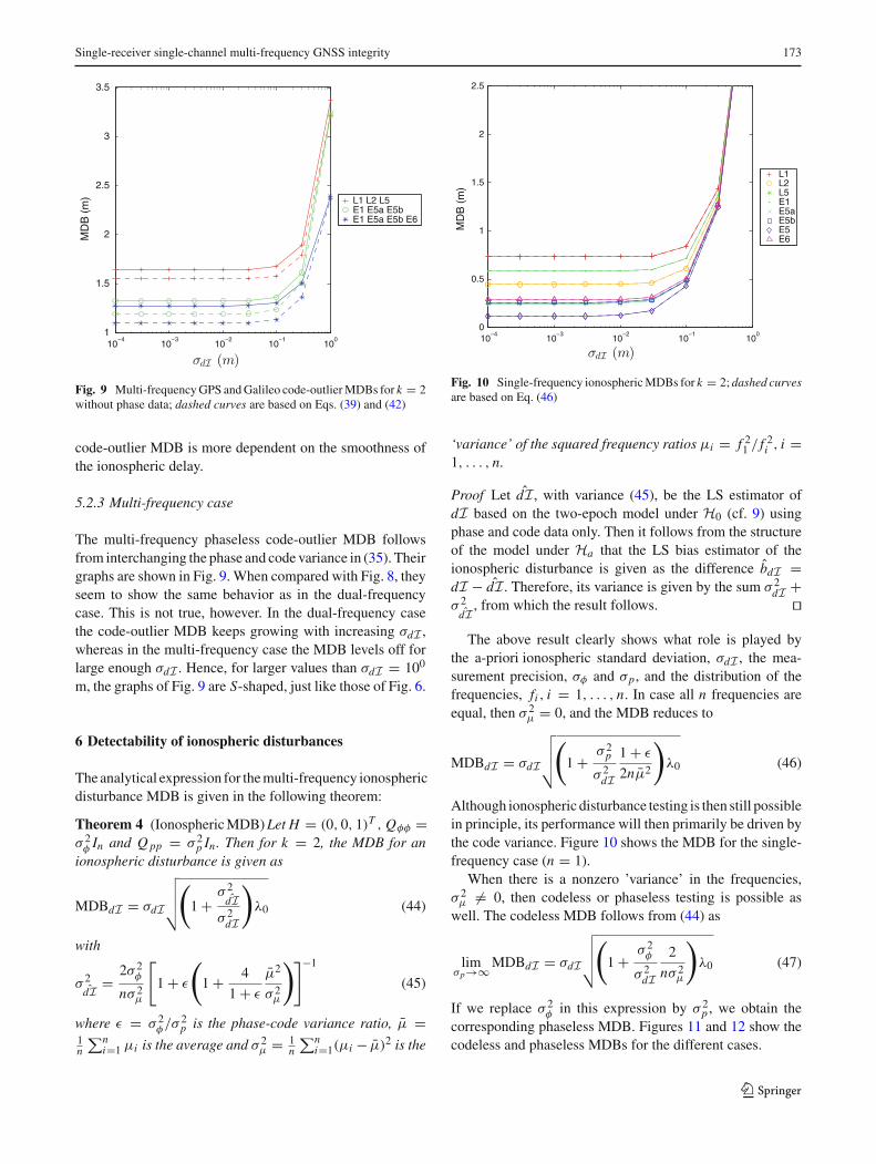
The multi-frequency phaseless code-outlier MDB followsfrom interchanging the phase and code variance in (35). Theirgraphs are shown in Fig. 9. When compared with Fig. 8, theyseem to show the same behavior as in the dual-frequencycase. This is not true, however. In the dual-frequency casethe code-outlier MDB keeps growing with increasing σdI ,whereas in the multi-frequency case the MDB levels off forlarge enough σdI . Hence, for larger values than σdI = 100

m, the graphs of Fig. 9 are S-shaped, just like those of Fig. 6.

6 Detectability of ionospheric disturbances

The analytical expression for the multi-frequency ionosphericdisturbance MDB is given in the following theorem:

Theorem 4 (Ionospheric MDB) Let H = (0, 0, 1)T , Qφφ =σ 2

φ In and Q pp = σ 2p In. Then for k = 2, the MDB for an

ionospheric disturbance is given as

MDBdI = σdI

√√√√(

1 +σ 2

ˆdIσ 2

dI

)λ0 (44)

with

σ 2ˆdI = 2σ 2

φ

nσ 2μ

[1 + ε

(1 + 4

1 + ε

μ2

σ 2μ

)]−1

(45)


p is the phase-code variance ratio, μ =1n

∑ni=1 μi is the average and σ 2

μ = 1n

∑ni=1(μi − μ)2 is the

10−4

10−3

10−2

10−1

100

0

0.5

1

1.5

2

2.5

MD

B (

m)

L1L2L5E1E5aE5bE5E6

Fig. 10 Single-frequency ionospheric MDBs for k = 2; dashed curvesare based on Eq. (46)

‘variance’ of the squared frequency ratios μi = f 21 / f 2

i , i =1, . . . , n.

Proof Let ˆdI, with variance (45), be the LS estimator ofdI based on the two-epoch model under H0 (cf. 9) usingphase and code data only. Then it follows from the structureof the model under Ha that the LS bias estimator of theionospheric disturbance is given as the difference bdI =dI − ˆdI. Therefore, its variance is given by the sum σ 2

dI +σ 2

ˆdI , from which the result follows. �

The above result clearly shows what role is played bythe a-priori ionospheric standard deviation, σdI , the mea-surement precision, σφ and σp, and the distribution of thefrequencies, fi , i = 1, . . . , n. In case all n frequencies areequal, then σ 2

μ = 0, and the MDB reduces to

MDBdI = σdI

√√√√(

1 + σ 2p

σ 2dI

1 + ε

2nμ2

)λ0 (46)

Although ionospheric disturbance testing is then still possiblein principle, its performance will then primarily be driven bythe code variance. Figure 10 shows the MDB for the single-frequency case (n = 1).

When there is a nonzero ’variance’ in the frequencies,σ 2

μ = 0, then codeless or phaseless testing is possible aswell. The codeless MDB follows from (44) as

limσp→∞ MDBdI = σdI

√√√√(

1 + σ 2φ

σ 2dI

2

nσ 2μ

)λ0 (47)

If we replace σ 2φ in this expression by σ 2

p , we obtain thecorresponding phaseless MDB. Figures 11 and 12 show thecodeless and phaseless MDBs for the different cases.

123


10−4

10−3

10−2

10−1

100

10−2

10−1

100

MD

B (

m)


Fig. 11 Dual- and multi-frequency codeless ionospheric MDBs fork = 2; dashed curves are based on Eq. (47)

10−4

10−3

10−2

10−1

100

1

1.5

2

2.5

3

3.5

4

MD

B (

m)


Fig. 12 Dual- and multi-frequency phaseless ionospheric MDBs fork = 2; dashed curves are based on Eq. (47), with code variance replacedby phase variance

7 Detectability of phase loss-of-lock

Phase loss-of-lock is defined as the simultaneous occur-rence of an unknown multivariate slip in all n carrier phaseobservables. To study its detectability, we first determine thevariance matrix of the multivariate slip under Ha and thenprovide bounds on the norm of the phase loss-of-lock MDB-vector.

7.1 The variance matrix of the multivariate slip

In the presence of a phase loss-of-lock, the design matrixof the alternative hypothesis (9) takes for k = l = 2 theform [G, H ], with H = [In, 0, 0]T . From the structure of

[G, H ], it follows that the carrier phase vector φ(t, s) willnot contribute to the estimation of the parameters ρ∗(t, s)and I(t, s) under Ha . These parameters are therefore solelydetermined by the code observables and a priori ionosphericinformation. As a consequence, the two-epoch bias esti-mator is given as the difference b = φ(t, s) − φ(t, s),where φ(t, s) = en ρ∗(t, s) − μI(t, s) is the least-squaresphase estimator based solely on the code observables anda priori ionospheric information. Solving for ρ∗(t, s) andI(t, s), followed by applying the variance propagation lawto b = φ(t, s) − en ρ∗(t, s) + μI(t, s) gives then the vari-ance matrix of the multivariate slip. The result is given in thefollowing Lemma:

Lemma 2 (Variance matrix of multivariate slip) For k =l = 2 and H = (In, 0, 0)T , the variance matrix of the least-squares estimator of b in (9) is given as

Qbb = 2Qφφ + 2Pen Q pp PTen

+ σ 2dI Ren μμT RT

en(48)

with σ 2dI =( 1

2μT Q−1pp P⊥

enμ+σ−2

dI )−1, P⊥en

= In − Pen , Pen =en(eT

n Q−1pp en)−1eT

n Q−1pp and Ren = In + Pen .

Note that the variance matrix is a sum of three matrices, theentries of which may differ substantially in size. The firstmatrix is governed by the precision of the phase observablesand will therefore have small entries. The second matrix isgoverned by the precision of the code observables and willtherefore have generally much larger entries than the firstmatrix in the sum. The third matrix depends, next to theprecision of the code observables, also on μ and σ 2

dI . Itsentries will become smaller if σ 2

dI gets smaller. This happens

for smaller σ 2dI (smoother ionospheric delays) and/or larger

μT Q−1pp P⊥

enμ (better code precision and/or larger frequency

diversity). Thus if σ 2dI = ∞, frequency diversity is needed

(i.e., μT Q−1pp P⊥

enμ = 0) so as to avoid the entries of the third

matrix in (48) to become infinite.We now discuss the detectability of the phase loss-of-lock

for n ≥ 2. The single-frequency case n = 1 is already treated(cf. 30), since phase loss-of-lock is then equivalent to havinga phase-slip.

7.2 Bounding the MDB vector

The variance matrix (48) can be used together with (25)to determine the phase loss-of-lock MDB-vector. Its lengthdepends on the direction d in which the multivariate slipoccurred,

||MDB|| =√

λ0

dT Q−1bb

d(49)

For certain directions, this may result in a short vector, whilefor other directions, it may be a long vector.

123


For its length, the following upper bound can be used:

||MDB|| ≤ σdT b

√λ0 (50)

where σ 2dT b

= dT Qbbd is the variance of dT b, with d beingthe unit vector that points in the direction of the slip. Theupper bound is easier to obtain as it avoids the inversion ofthe variance matrix (48).

Considering (48), it is not difficult to see in which direc-tions the MDB-vector will be short. If d ⊥ en , then PT

end = 0,

meaning that the second term of (48) will not contribute. Andif d ⊥ span{en, μ}, then RT

end = 0 and PT

end = 0, meaning

that now also the third term will not contribute. Thus

||MDB|| ≤√

2λ0dT Qφφd if d ⊥ span{en, μ} (51)

This shows that the length of the MDB vector is verysmall indeed if d lies in the (n − 2)-dimensional spacespan{en, μ}⊥. In this case, the phase loss-of-lock has verygood detectability, since the MDB is then solely driven bythe very precise carrier phase data.

The situation changes drastically, however, if d is takento lie in span{en, μ}. In that case the large code variancedependent second and third term of (48) will contribute aswell. The largest possible value that the length of the MDBvector can take corresponds with d being the eigenvector ofQbb with largest eigenvalue. The corresponding bounds forthe ionosphere-fixed and ionosphere-float case are given inthe following Lemma:

Lemma 3 (Phase loss-of-lock MDB upper bounds) LetQφφ = σ 2

φ In, Q pp = σ 2p In. Then

||MDB|| ≤⎧⎨⎩

σp√

2(1 + ε)λ0 if σ 2dI = 0

σp

√2(

1 + ε + 2√f −1

)λ0 if σ 2

dI = ∞ (52)

with f = 1 +(

σμ

μ

)2, where σ 2

μ = 1n

∑ni=1(μi − μ)2 and

μ = 1n

∑ni=1 μi .

Proof see Appendix. �

The ionosphere-fixed upper bound corresponds with a slipin the en-direction, while the ionosphere-float upper bound

corresponds with a slip in the direction en +√

n||μ||μ. Thus

phase loss-of-lock is most difficult to detect if it results ina slip with such direction. For example, for the ionosphere-fixed, dual- and triple-frequency (q = 2, 3) cases, the lengthof the MDB-vector will then be about six to seven times thecode standard deviation.

To conclude, we note that we can apply the duality of phaseand code to the above lemma and so obtain directly also thelength of the MDB vector ||MDB||p that corresponds to thecase that the complete n-dimensional code vector is outlying.

By interchanging the phase- and code variance in (52), weobtain

||MDB||p ≤⎧⎨⎩

σp√

2(1+ε)λ0 if σ 2dI =0

σp

√2(

1+ε(1+ 2√f−1

))

λ0 if σ 2dI =∞

(53)

The ionosphere-fixed upper bound is the same as in (52),but the ionosphere-float upper bound differs. In this secondbound we note that the effect of frequency diversity (i.e., theeffect of f ) gets reduced due to its multiplication with thesmall phase-code variance ratio ε. This corresponds to ourearlier findings in Sect. 5.1.2, where it was stated that overthe considered range of σ 2

dI , the code-outlier MDB is muchmore insensitive to frequency diversity than the phase-slipMDB is.

8 Summary and conclusions

In this contribution we presented an analytical and numericalstudy of the integrity of the multi-frequency single-receiver,single-channel GNSS model. The UMPI test statistics forspikes and slips are derived and their detection capabilitiesare described by means of the concept of minimal detectablebiases (MDBs). Analytical closed-form expressions of thephase-slip and code outlier MDBs have been given, thus pro-viding insight into the various factors that contribute to thedetection capabilities of the various test statistics. This wasalso done for the phaseless and codeless cases, as well as forthe case of loss-of-lock.

The MDBs were evaluated numerically for the severalGPS and Galileo frequencies. From these analyses it canbe concluded that detectability of dual- and triple-frequencyphase-slips works well for k = l = 2. Single-frequencyphase-slip detectability, however, is problematic, thus requir-ing more epochs of data.

From the codeless phase-slip MDBs it follows thatdetectability is not possible in the single-frequency case, butthat it is possible for the dual- and triple-frequency cases. Inthe dual-frequency case the codeless phase-slip MDBs areless then 10 cm if σdI ≤ 3 cm, while for the triple-frequencycase this is already true for σdI ≤ 1 m. In the triple-frequencycase, the phase-slip MDBs get even as small as a few cen-timeters if σdI ≤ 3 cm. These codeless results are importantas it shows that in the presence of code multipath, one cando away with the code data and then still have integrity forphase slips.

The code outlier MDBs are, except for the single-frequency case, all relatively insensitive to the smoothnessof the ionosphere. The effect of the frequencies is also hardlypresent in the multi-frequency code-outlier MDBs. Theirvalue is predominantly determined by the precision of thecode measurements. From the phaseless code-outlier MDBs

123


it follows that, except for the single-frequency case, code out-lier detection is still possible. The multi-frequency phaselesscode-outlier MDBs all lie around 1 m for σdI ≤ 10 cm. Theyincrease rapidly, however, for larger values of σdI .

Acknowledgments The first author is the recipient of an Aus-tralian Research Council (ARC) Federation Fellowship (project numberFF0883188). Part of this work was done in the framework of the project‘New Carrier-Phase Processing Strategies for Next Generation GNSSPositioning’ of the Cooperative Research Centre for Spatial Information(CRC-SI2). The work of the second author was partly supported by theEU Marie Curie program in the framework of the FP7-PEOPLE-IAPP-2008 (SIGMA) project. All this support is gratefully acknowledged.

Open Access This article is distributed under the terms of the CreativeCommons Attribution License which permits any use, distribution, andreproduction in any medium, provided the original author(s) and thesource are credited.

9 Appendix

Proof of Theorem 1 (UMPI test statistic): First we prove(13). Define

A = (A1, A2) = (Ik−1 ⊗ G, DTk sl ⊗ H)

W = (DTk Dk)

−1 ⊗ Q−1

x = (dgT , bT )T

(54)

Reduction of the system of normal equations AT W Ax =AT W y for b gives AT

2 W A2b = AT2 W y and thus

b = ( AT2 W A2)

−1 AT2 W y, Qbb = ( AT

2 W A2)−1 (55)

with A2 = P⊥A1

A2 and P⊥A1

= I − A1(AT1 W A1)

−1 AT1 W .

With the use of (54) in (55), the result (13) follows.For the UMPI test statistic, we have Tq = bT Q−1

bbb =

yT W AT2 ( AT

2 W A2)−1 A2W y. With the use of (54), this

expression reduces to (14). �Proof of Theorem 2 (Phase-slip MDB): For an MDB withk = l = 2, we have, with q = 1 (i.e., d = ±1), according to(25) and (15),

MDB =√

2λ0

H T Q−1 P⊥G H

(56)

For a phase-slip MDB we have H = (δTj , 0T , 0T )T , Q =

blockdiag(σ 2φ In, σ 2

p In, 12σ 2

dI) and P⊥G = In−G(GT Q−1G)−1

GT Q−1. Substitution into (56) gives the phase-slip MDB as

MDBφ j = σφ

√2λ0

1 − 1n∗

(57)

with 1n∗ = δT

j G(GT σ 2φ Q−1G)−1GT δ j . A further simplifi-

cation of this scalar expression gives (29). �

Proof of Theorem 3 (Phase loss-of-lock MDB upper bounds):We give the proof for the ionosphere-fixed case. For theionosphere-float case it goes along similar lines.

To determine the eigenvalues of Qbb (c.f. 48) for Qφφ =σ 2

φ In, Q pp = σ 2p In and σ 2

dI = 0, we need to determine theroot γ of

|2σ 2φ In + 2σ 2

pe(eT e)−1eT − γ In| = 0 (58)

Let D be an n × (n − 1) basis matrix of the orthogonalcomplement of e. Then the n × n matrix M = [D, e] is offull rank. Pre- and post-multiplication of the matrix in (58)with MT and M allows to reduce the determinantal equationinto a product,

|(2σ 2φ − γ )DT D| |(2σ 2

p − γ )n + 2σ 2pn| = 0 (59)

This shows that there are (n − 1) eigenvalues with the valueγ = 2σ 2

φ and one eigenvalue, the largest, with the value

γ = 2(σ 2φ + σ 2

p) = 2σp(1 + ε). Hence, for the MDB upperbound we get

||MDB||φ ≤ √γmaxλ0 = σp

√2(1 + ε)λ0 (60)

This concludes the proof. �

References

Arnold SF (1981) The theory of linear models and multivariate analysis.Wiley, New York

Baarda W (1967) Statistical concepts in geodesy. Netherlands GeodeticCommission, Publications on Geodesy, New Series 2(4)

Baarda W (1968) A testing procedure for use in geodetic networks.Netherlands Geodetic Commission, Publications on Geodesy, NewSeries 2(5)

Bisnath SB, Langley RB (2000) Efficient, automated cycle-slip cor-rection of dual-frequency kinematic GPS data. In: Proceedings IONGPS 2000, pp 145–154

Bisnath SB, Kim D, Langley RB (2001) Carrier phase slips: a newapproach to an old problem. GPS World, May 2001, pp 2–7

Blewitt G (1998) GPS for geodesy. In: Teunissen PJG, Kleusberg A(eds) GPS data processing methodology. Springer, Berlin

Collins JP, Langley RB (1999) PossibleWeighting schemes for GPScarrier phase observations in the presence of multipath. Universityof New Brunswick

Dai Z, Knedlik S, Loffeld O (2009) Instantaneous triple-frequency GPScycle-slip detection and repair. Int J Navig Observ, p 15. doi:10.1155/2009/407231

de Bakker PF (2011) Modeling pseudo range multipath as an autore-gressive process. In: Proceedings of ION GNSS 2011, pp 1737–1750

de Bakker PF, van der Marel H, Tiberius CCJM (2009) Geometry-free undifferenced, single and double differenced analysis of singlefrequency GPS. EGNOS and GIOVE-A/B measurements, GPS Solut

de Bakker PF, Tiberius CCJM, van der Marel H, van Bree RJP (2012)Short and zero baseline analysis of GPS L1 C/A, L5Q, GIOVE E1B,and E5aQ signals. GPS Solut

de Jong K (2000) Minimal detectable biases of cross-correlated GPSobservations. GPS Solut 3:12–18

de Jong K, Teunissen PJG (2000) Minimal detectable biases of GPSobservations for a weighted ionosphere. Earth Planets Space 52:857–862

123

http://dx.doi.org/10.1155/2009/407231

http://dx.doi.org/10.1155/2009/407231


de Jong K, van der Marel H, Jonkman NF (2001) Real-time GPS andGLONASS integrity monitoring and reference station software. PhysChem Earth (A) 26(6–8):545–549

De Lacy MC, Reguzzoni M, Sanso F (2011) Real-time cycle slipdetection in triple-frequency GNSS. GPS Solut. doi:10.1007/s10291-011-0237-5

Euler H-J, Goad CC (1991) On optimal filtering of GPS dual frequencyobservations without using orbit information. Bull Geod 65:130–143

Fan J, Wang F, Guo G (2006) Automated cycle-slip detection and cor-rection for GPS triple-frequency undifferenced observables. J SciSurveying Mapping 31(5):24–36

Fan L, Zhai G, Chai H (2011) Study on the processing method ofcycle-slips under kinematic mode. In: Zhou Q (ed) ICTMF2011,pp 175–183

Feng S, Ochieng WY, Walsh D, Ioannides R (2006) A measurementdomain receiver autonomous integrity monitoring algorithm. GPSSolut 10:85–96

Foerstner W (1983) Reliability and discernability of extended Gauss-Markov models. In: German geodetic commission DGK, Series A,No. 98, pp 79–103

Gao Y, Li X (1999) Cycle slip detection and ambiguity resolutionalgorithms for dual-frequency GPS data processing. Mar Geod22(4):169–181

Giorgi G, Teunissen PJG, Verhagen S, Buist PJ (2012) Instantaneousambiguity resolution in GNSS-based attitude determination appli-cations: a multivariate constrained approach. J Guid Control Dyn35(1):51–67

Hartinger H, Brunner FK (1999) Variances of GPS phase observations:the SIGMA model. GPS Solut 2(4):35–43

Hewitson S, Wang J (2006) GNSS receiver autonomous integrity mon-itoring (RAIM) performance analysis. GPS Solut 10:155–170

Hewitson S, Wang J (2010) Extended receiver autonomous integritymonitoring for GNSS/INS integration. J Surv Eng 2010:13–22

Hofmann-Wellenhoff B, Lichtenegger H (2001) Global positioning sys-tem: theory and practice, 5th edn. Springer, Berlin

Jonkman NF, de Jong K (2000) Integrity monitoring of IGEX-98 data,Part II: cycle slip and outlier detection. GPS Solut 4(3):24–34

Knight NL, Wang J, Rizos C (2010) Generalised measures of reliabilityfor multiple outliers. J Geod 84:625–635

Koch KR (1999) Parameter estimation and hypothesis testing in linearmodels. Springer, Berlin

Kok JJ (1982a) Statistical analysis of deformation problems usingBaarda’s testing procedures. In: Daar heb ik veertig jaar overnagedacht, Festschrift Willem Baarda, Part 2, Delft, pp 469–488

Kok JJ (1982b) On data snooping and multiple outlier testing. Technicalreport National Geodetic Survey, NOAA/NOS

Langley R (1997) GPS receiver system noise. GPS World 8:40–45Leick A (2004) GPS satellite surveying. Wiley, New YorkLipp A, Gu X (1994) Cycle slip detection and repair in integrated naviga-

tion systems. In: Proceedings IEEE PLANS94, pp 681–688. doi:10.1109/PLANS.1994.303377

Liu Z (2010) A new automated cycle-slip detection and repair methodfor a single dual-frequency GPS receiver. J Geod. doi:10.1007/s00190-010-0426-y

Liu X, Tiberius CCJM, de Jong K (2004) Modelling of differentialsingle difference receiver clock bias for precise positioning. GPSSolut 4:209–221

Mertikas SP, Rizos C (1997) On-line detection of abrupt changes in thecarrier-phase measurements of GPS. J Geod 71:469–482

Miao Y, Sun ZW, Wu SN (2011) Error analysis and cycle-slip detectionresearch on satellite-borne GPS observation. J Aerosp Eng 24(1):95–101

Misra P, Enge P (2001) Global positioning system: signals, measure-ments, and performance. Ganga-Jamuna Press, Lincoln

Rao CR (1973) Linear statistical inference and its applications. Wiley,New York

Salzmann M (1991) MDB: a design tool for integrated navigation sys-tems. J Geod 65(2):109–115

Simsky A, Mertens D, Sleewaegen J-M, De Wilde W, Hollreiser M,Crisci M (2008) MBOC vs. BOC(1,1) mulipath comparison basedon GIOVE-B data. Inside GNSS, September/October, pp 36–39

Teunissen PJG (1986) Adjusting and testing with the models of theaffine and similarity transformation. Manuscr Geod 11:214–225

Teunissen PJG (1990a) Quality control in integrated navigation systems.IEEE Aerosp Electron Syst Mag 5(7):35–41

Teunissen PJG (1990b) An integrity and quality control procedurefor use in multi-sensor integration. In: Proceedings ION GPS-90,pp 513–522. Also in: Red book series of the Institute of Navigation,2012, vol VII

Teunissen PJG (1997) GPS double difference statistics: with and with-out using satellite geometry. J Geod 71:137–148

Teunissen PJG (1998a) GPS for geodesy. In: Teunissen PJG, KleusbergA (eds) Quality control and GPS. Springer, Berlin

Teunissen PJG (1998b) Minimal detectable biases of GPS data. J Geod72:236–244

Teunissen PJG (2000) Testing theory: an introduction. Delft UniversityPress, VSSD

Teunissen PJG, Kleusberg A (1998) GPS for geodesy, 2nd edn. Springer,Berlin

Van Mierlo J (1980) A testing procedure for analytic deformationmeasurements. In: Proceedings of internationales symposium ueberDeformationsmessungen mit Geodaetischen Methoden. Verlag Kon-rad Wittwer, Stuttgart

Van Mierlo J (1981) A review of model checks and reliability. In: Pro-ceedings of VIth international symposium on geodetic computations,Munich

Ward P (1996) Satellite signal acquisition and tracking. In: Kaplan ED(ed) Understanding GPS: principles and applications. Artech House,Boston

Wieser A, Petovello MG, Lachapelle G (2004) Failure scenarios to beconsidered with kinematic high precision relative GNSS positioning.In: Proceedings ION GNSS

Wieser A, Gaggl M, Hartinger M (2005) Improved positioning accuracywith high-sensitivity GNSS receivers and SNR aided integrity mon-itoring of pseudo-range observations. In: Proceedings ION GNSS2005, pp 1545–1554

Wu Y, Jin SG, Wang ZM, Liu JB (2010) Cycle-slip detection usingmulti-frequency GPS carrier phase observations: a simulation study.Adv Space Res 46:144–149

Xu D, Kou Y (2011) Instantaneous cycle slip detection and repair fora standalone triple-frequency GPS receiver. In: Proceedings 26thITM-ION, pp 3916–3922

123

http://dx.doi.org/10.1007/s10291-011-0237-5

http://dx.doi.org/10.1007/s10291-011-0237-5

http://dx.doi.org/10.1109/PLANS.1994.303377

http://dx.doi.org/10.1109/PLANS.1994.303377

http://dx.doi.org/10.1007/s00190-010-0426-y

http://dx.doi.org/10.1007/s00190-010-0426-y

single-receiver single-channel multi-frequency gnss

Documents