single particle dynamics in i ,;‘ -. circular accelerators · pdf filesingle particle...

SLAC - PUB - 4103 October 1986 (4

SINGLE PARTICLE DYNAMICS IN i ,;‘ -. CIRCULAR ACCELERATORS

. Ronald D. Ruth

Stanford Linear Accelerator Center Stanford University, Stanford, CA 94305

TABLE OF CONTENTS

-

1. Introduction .............................

2. Hamiltonian Dynamics ........................ 2.1 Equations of Motion ....................... 2.2 Symmetry, Integrals and Invariant Tori ............. 2.3 Motion Near a Known Periodic Solution ............

3. Canonical Transformations ..................... 3.1 The Generating Function .................... 3.2 Action-Angle Variables for the Harmonic Oscillator ....... 3.3 Deviation From a Known Solution ...............

4. The Motion of a Particle in an Accelerator ............. 4.1 The Hamiltonian and the Equations of Motion .........

_ . .._ . 4.2 The Coordinate System and the Change of Independent Variable - 4.3 The Linearized Equations of Motion ..............

5. Linear Equations with Periodic Coefficients ............ .-. 5.1 The Matrix Approach ......................

5.2 The Phase-Amplitude Form of the Solution .......... 5.3 Action-Angle Variables ..................... 5.4 Adiabatic Damping ....................... 5.5 The Adiabatic Invariance of the Action .............

6. The Nonlinear Terms ........................ 6.1 The Sources of Nonlinearity and Chromaticity ..........

_ . ._n. 6.2 Sextupoles for Chromatic Correction .............. - ;. 7. Canonical Perturbation Theory ................... -

7.1 The Equation for the Generating Function ........... -_ 7.2 The Solution for the Generating Function ...........

7.3 The New Hamiltonian and the Amplitude Dependence of the Tune

*Work supported in by the Department of Energy, contracts DEAC03-76SF00515

3

9 9

11 13

14 14 15 17

18 19 23 26 29 30

32 32 4

33

35 35 36 37

Invited talk presented at the 1985 SLAC Summer School on the Physics of

High Energy Particle Accelerators, Stanford, California, July 15-26, 1985

8. Linear Perturbations ........................ 39 . ,=-- 8.1 Qaadrupole Gradient Perturbation ... .; ........... 39

. 8.2 Weak Linear Coupling ..................... 41

9.. A Sextupole Perturbation . . . . . . . . . . . . . . . . . . . . . . 43

10. An Isolated Resonance in One Degree of Freedom ........ 45 10.1 Fixed Points .......................... 46 10.2 Resonance Island Width .................... 47 10.3 Island Separation and the Chirikov Criterion ......... 48 10.4 Island ‘Tune’ and Green’s Residue Criterion ......... 49 10.5 Unbounded Motion ...................... 51

11. A Isolated Resonance in Two Degrees of Freedom ......... 52 11.1 Calculation of the Invariants .................. 52

- 11.2 Viewing Coupled Motion ................... 54 -

-

12. The Residue Criterion ....................... 58 12.1 The Definition of the Residue ................. 58 12.2 Continued Fractions ...................... 59 12.3 A Precise Statement of the Residue Criterion ......... 60

-12.4 An Isolated Resonance Example ................ 60

13. Direct Solution of the Hamilton-Jacobi Equation ......... 61 13.1 The Hamilton-Jacobi Equation ................ 62

_._._ . 13.2 An Integrable Example .................... 64 - 13.3 The Two Resonance Model .................. 65

13.3.1 A New Criterion for the Break-up of a KAM curve . . 66 13.3.2 Invariant Curves and Their Break-up ......... 67

-- 13.4 A Comparison with the Residue Criterion ........... 70

14. Renormalization: The Route to Chaos . . . . . . . . . . . . . . 72 14.1 The Two Resonance Model . . . . . . . . . . . . . . . . . . 73

14.1.1 Scaling the Time and the Momentum . . . . . . . . . 73 14.1.2 The ‘Standard’ Form of the Two Resonance Model . . 74

14.2 The Renormalization Transformation . . . . . . . . . . . . . 76 14.3 The Renormalization Group . . . . . . . . . . . . .- . . . . . 80 .G

_. _ _Y. 14.4 A Discussion of Renormalization . . . . . . . . . . . . . . . 84 ~-- L.

15. Acknowledgements . . . . . . . . . . . . . . . . . . . . . . . . . 84

15. References . . . . . . . . . . . . . . . . . . . . . . . . . . . . . 85

-. k.

1. INTRODUCTIO N

The purpose of this paper is to introduce the reader to the theory assoc iated with the transverse dynamic s of s ingle partic les in c ircu lar accelerators. Since the treatment here uses the Hamiltonian formulation of dynamic s , the discuss ion begins with a review of Hamiltonian dynamic s and canonical transformations.

Next we specialize to the case of a partic le in a c ircu lar accelerator and develop the equations of motion from the relativ is tic Hamiltonian for a partic le in an elec tromagnetic field. This leads to the linearization of the motion about a c losed orbit. Temporarily suppressing the nonlinear terms, we then give a s tandard treatment of linear equations with periodic coefficients which leads to a discuss ion of betatron osc illations .

-

-

The solution of the linearized equation leads naturally to the action-angle var iables for that problem. These var iables form the basis for the s tudy of the higher order nonlinear terms. Before analy z ing these terms we discuss briefly the sources of nonlinearity and motivate the inc lus ion of seztupoles in a c ircu lar accelerator or s torage ring for the control of the chromaticity, the momentum dependence of the betatron frequency or tune.

In the next sect ion a general formulation of canonical perturbation theory is presented. This leads to some examples of the technique for linear pertur-

_. .- . bations and for a sextupole perturbation. Perturbation theory breaks down in - the neighborhood of resonances. However, for an iso lated resonance there is an alternative approach which y ields the basic s tructure in phase space. To demonstrate this we treat a s ingle resonance, ca lcu late the exact invar iants and illus trate the s tructure in phase space.

Unfortunately this technique gives an exact answer only for one resonance. For multiple resonances one must face the non-integrability of nonlinear equations in general. This leads to a brief discuss ion of the Chirikov c r iterion and Greene’s residue c r iterion as methods for estimating the onset of chaotic behavior in phase space.

-

To complete the discussion of nonlinear resonances we go to the case of two r- degrees of freedom. Once again the case of an isolated nonlinear resonance is

. studied; the invariants are calculated and methods for the projective viewing of the invariant torus are presented. This concludes the more standard part of the paper.

In the next few sections a more in depth treatment of the questions of chaotic behavior and the breaking of KAM curves is presented. This begins in Section 12 with a discussion of the residue criterion to set the stage for the next two sections.

In the next section recent work is presented on the direct calculation of KAM curves avoiding perturbation theory. This leads to a new criterion for the break-up of a KAM curve which is then compared in some detail with the residue criterion converted to the language of canonical transformations.

In the last section we discuss the concept of renormalization as a technique for determining the break-up of a KAM curve. This section focuses on the discussion of an example which is presented in detail. However, this gives quite general results due to the universal nature of renormalization and the residue criterion. This final section concludes with a calculation of the critical residue for-the breaking of a KAM curve and a discussion of the structure of the self-

- similarity revealed by the renormahzation approach.

Many important subjects are only mentioned briefly here and some are not discussed at all. Since the focus is on single particle dynamics, all collective -. .- . - effects are neglected. It is usual to treat collective effects as a perturbation to the single particle dynamics.

-. In addition we neglect the difference between electrons and protons in this

treatment. Issues relating to damping due to synchrotron radiation, quantum excitation, etc. are treated elsewhere in these proceedings. However, since the time scale for damping in an electron storage ring is very long compared to both the revolution period and the betatron oscillation period, the results obtained here are quite relevant to electrons as well as protons.

The discussion is also confined to transverse dynamics ignoring longitudinal dynamics and synchrqtrqn oscillations. Typically the synchrotron frequency is

_. _ -1. quite small compared to the betatron frequency and thus there is a natural - ._ cseparation here. This not to say, however, that the general-results obtained in

many of the sections cannot be applied to synchrotron oscillations. In particular, - the discussion of resonances is quite relevant and leads in this case to synchro- betatron resonances.

Finally, the discussion of methods for determining the transition of chaotic behavior or the breaking of a KAM curve are somewhat brief but reasonably up to date. The field of nonlinear dynamics is a rapidly advancing one; here we

-

4

i concentrate on those features which might have useful applications in accelerator r- theory. -. --

. The primary references for introductory part of this paper (Sections 1 - 11) are Refs. 1 and 2. References for the sections dealing with the transition to chaotic behavior (Sections 12 - 14) will be given in the appropriate sections.

2. HAMILTONIAN DYNAMICS

2.1 EQUATIONS OF MOTION

The dynamical systems of interest here can be described by a Hamiltonian H(q,p, t). q is the coordinate, p is the canonical momentum, and t is the independent variable or time. In many cases the Hamiltonian is the sum of the kinetic energy T and potential energy V each written as a function of the coor-

- dinates and canonical momenta. The equations of motion can be derived from the Hamiltonian using Hamilton’s equations:

-

dq; c.3H dpi aH -- dt - api ’ dt = -aqi . (24

For example, consider a system of ?t nonrelativistic particles interacting through a force law derivable from a potential. Then we have

H=$--(p;+p;+ -+P3 +V(!n, !72,-,Qn) (2.2) - .- . - and

hi pi dpi w dt=; 9 dt=-aqi, P-3)

-- The above differential equations are simply Newton’s Second Law for the n-particle system.

In the above example the canonical momenta were equal to the kinetic momenta. It is evident that this is not true for more general Hamiltonians. Con- sider for example a nonrelativistic charged particle in an electromagnetic field with vector potential A(z, t) and scalar potential a(~, t). Then the Hamiltonian is given by

H = & (p- fA(x,t))‘+e@(x,t) - (2.4 L.

and the corresponding equations of motion are

dxi pi - :A,. V’Edt= m

(24

-

dpi d@ e dt=+azi-, c

(pi - ;Ai) ilAi

i m dz;’

5

i Note that in this case the canonical momenta and the kinetic momenta are

r-- related by -- . mvi = pi - CAi .

c (2.6)

To convert the equations of motion to more conventional form recall the relations relating the electric and magnetic fields to the vector and scalar potentials,

B=VxA

E-V+=. P-7)

Using Eq. (2.6) t o eliminate the canonical momenta in favor of the velocities, Eq. (2.5) becomes

- dv e dt=m {E+LB} .

c (2.8) Equation (2.8) is simply the Lorentz force equation for a nonrelativistic charged particle in an external electromagnetic field.

2.2 SYMMETRY, INTEGRALS, AND INVARIANT TORI -

If we examine Eq. (2.3), 't 1 is easy to see that if the Hamiltonian is independent of some coordinate qm, then the corresponding canonical momentum

_._._ . p, is a constant of the motion. In this case p, is a first integral of the motion - and the coordinate qm is called a ‘cyclic’ or ‘ignorable’ coordinate. In general, the existence of such an integral corresponds to a certain symmetry of the system. In this case the symmetry is the invariance of the equations of motion to translations in qm. If qm is an angular coordinate, then the conjugate angular momentum is conserved, and the system is invariant with respect to a rotation in qm.

In general for an n-dimensional system, Hamilton’s equations constitute a system of 2n ordinary first-order differential equations. In order to integrate such a system we need to know 2n first integrals. In many cases, however, it is sufficient to know only n independent integrals. In these-cases each inte-

_ _-. gral can be used to reduce the order of the system of equations by two rather - ._ -than just one. These problems are.called integrable, and -the motion is con-

fined to an n-dimensional surface in 2n-dimensional phase space. In the case - of bounded oscillatory motion, the motion is confined to n-dimensional torus in

2n-dimensional phase space.

In other cases n independent integrals do not exist; these are called nonintegrable. In these cases the trajectory can fill regions of phase space of dimension greater than n. In these nonintegrable cases there are, however, invariant tori

-

6

-.-.. . -

as shown by KAM (Kolmogorov, Arnold, and Moser).3 These invariant tori, however, ?lo ‘not exist as continuous families as in the integrable case. The set of invariant tori is a Cantor set. Just next to each invariant torus is a region of resonance and chaotic behavior. In spite of this for nonintegrable systems which differ from integrable ones only by the addition of small nonlinear terms, there are invariant tori almost everywhere in phase space.

The case of two degrees of freedom with a time independent Hamiltonian is a special one because the torus is 2-dimensional (a real donut), but the phase space is reduced to S-dimensions by the invariance of the Hamiltonian. Thus, the invariant tori ‘hold water’ in that they enclose volume in phase space. Therefore, the existence of KAM invariant tori in the case above (sometimes called If degrees of freedom) guarantees stability: Those orbits, whether chaotic or not, which are inside the donut must remain inside. If they were to ‘attempt’ to cross they would fall on the invariant tori. But since it is invariant they have been and will be on the invariant torus forever. Thus, in this case there are no orbits which connect the 3-dimensional volume inside the 2-torus to the 3-dimensional volume outside. This is not true, however, in systems of three or higher degrees of freedom. In these systems invariant tori do not guarantee stability since their dimensionality is too low to enclose volume. This leads to the phenomenon of Arnold difusion.

Although many of the differential equations which will be discussed here are, strictly speaking, nonintegrable, they are sufficiently close to integrable systems to admit approximate solutions. In cases where there is significant chaotic behavior it is necessary to use other techniques such as the residue criterion, the Chirikov criterion, the direct calculation of KAM tori through solution of the Hamilton-Jacobi equation, or renormalization techniques. These methods are concerned with the nature of the break-up of invariant tori and are discussed in Sections 12-14.

2.3 MOTION NEAR A KNOWN PERIODIC SOLUTION

In many cases we are interested in the orbits of a system which are close to a known periodic solution. This periodic solution may or may not be easy to find; let us assume that -we know it. Consider the Hamiltonian in Eq. (2.2) in

_. _ -2. two dimensions. This yields the equations of motion,

L. . . f3V

- mx=-z-

-

A periodic orbit x0(t) and ye(t) with period T is defined to be one which closes

7

on itself in time 2’. Thus it is defined by ‘ ,x.- -. -. .

mz0 = --t&0, ~0) , xo(t + T) = x0(t)

m50 = -~(xo, ~0) , Yo(t+T) = Ye(t) -

Now consider an orbit close to the periodic orbit and let

[=x-x0

- Substituting into Eq. (2.9) and expanding for small [ and 7, we find

6W mi = -t- ax2 (XOYYO) - rl @V

-(x0, Yo) axay

mf = -t -&(x0, Yo) - &o, Yo) *

(2.10)

(2.11)

(2.12)

Thus, since yc and x0 are periodic functions of t, we find a linear differential equation with periodic coefficients which can be derived from the Hamiltonian,

_. ..- . -

H= (2.13)

where the derivatives of the potential are again evaluated at (x0, ~0). Note that the coefficients in the new Hamiltonian now depend periodically on time rather than being constant. Therefore, the solutions will differ substantially from those for the harmonic oscillator.

The stability or instability of the periodic orbit in question is determined by the solutions of Eq. (2.12). Thus the solutions of linear equations with periodic coefficients are evidently of fundamental importance. The solutions to this type

_. _ _T_ of equation (Hill’s equation) in one degree of freedom will be discussed in Section - .- -a L.

-

8

3. CANONICAL TRANSFORMATIONS r -. -.

. A dynamical system is described in terms of a certain set of variables, coordinates and canonically conjugate momenta. Sometimes it is more convenient to -express the equations of motion in terms of different variables which are functions of the old ones. It is desirable to have the new coordinates again in Hamiltonian form; that is, if Q and P are the new coordinates, then

dQ aK(QJ’,t) dP dt= dP

aK (Q&t) , dt=- aQ (3.1)

where K(Q, P, t) is the new Hamiltonian. The question is then to find those transformations which accomplish this.

- 3.1 THE GENERATING FUNCTION OF A CANONICAL TRANSFORMATIONS

-

Hamilton’s equations of motion can be derived from a variational principle. For a system described by a Hamiltonian H(q,p, t), the Lagrangian function is

- L((a,Q,t) = c~iii - H(qi,pi,t) . (3.2) i

- . . . .- . Consider the evolution of the system from tl to t2 and the action integral -

ta S = ~(q(t),dt),t)dt . J

t1

(34 Next vary the function q(t) so that the end points are fixed, and ask for what q(t) is the action integral stationary. The answer can be found from the calculus of variations; q(t) must satisfy

_ _F_ d aL: aL o ----= dt ai aq

L.

(3.4) c ~--

which is equivalent to .-

d(pi) + aH o . aH - = dt aqi 3 Qi = api - (3.5)

Equations (3.5) are Hamilton’s equations of motion.

9

Now, with new variables Q and P and a new Hamiltonian K, Hamilton’s r- principle must again be valid

6 S’=6 i’ [c Pi& - K(Q, P,t)] dt = 0 .

t1 i

Therefore, the new and old Langrangian can differ at most by the total time derivative of some function W (recall that the end points are fixed).

.This function must be a function of the new and old variables. However, only 2n of these are independent for an n-dimensional problem since there are 2n transformation equations relating the new and old coordinates and momenta. Consider a function which depends only on the new and old coordinates. That is

- W = F&,Q,t) . (3.7)

Then we must have

Cpi(ji-H=CPii)i-K+z s

i i P-8)

- Now if we expand the total time derivative we have

_. .- . * T,(pi-!$-)-TQi (,+g)-(H-K+$)=O - (3-g)

For Eq. (3.9) to hold identically, the coefficients of 4 and Q must vanish because q and Q are the 2n independent variables. Thus we must have

aJ’1 pi = &li '

(3.10) W K=H + - at ’

_ _T_

-

Equations (3.10) specify the relations between the old and new variables in a canonical transformation. The first two of these equations can be solved for q and p in terms of Q,and P. The new Hamiltonian is then. given by the third equation in (3.10),

=‘I K(Q,W) = H(q(Q,P,t),p(Q,P,t),t) + dt (a(QJ’AQ,t) - (3.11)

-

C

Fl (q, Q, t) is called the generating function of the canonical transformation in Eqs. (3.10). Rather than choosing the old coordinates and new coordinates

10

._ (q,Q) as variables, we could have chosen the old coordinates and new momenta i .‘- (q, P). In th 1s case we have a different generatingjfunction &(q, P, t), and a

. different set of equations for the canonical transformation

P= $ (q&t) ,

Q=$ W,t) , (3.12)

K=H -I- T (q,P,t) -

F2 and Fl are related by a Legendre transformation.

The equations of a canonical transformation can be viewed in many different ways. We could start with the relationship between the coordinates, derive the generating function which yields that, and then find the new momenta and new Hamiltonian. Alternatively we could begin with a new Hamiltonian, solve for the generating function and then calculate the new coordinates. In the next sections we show some examples.

3.2 ACTION-ANGLE VARIABLES FOR THE HARMONIC OSCILLATOR

_._._ . * In this section we consider a problem that we know how to solve. The harmonic oscillator Hamiltonian is

w2x2 -- H=;+T,

and the solution of the equation of motion is

(3.13)

x = acos(wt + q5)) (3.14)

p = --a w sin(wt + rjc) ,

- &ere a and ~$0 are two arbitrary constants. The motion is confined to an ellipse in phase space. Note that the Hamiltonian is independent of the time and is thus

- a constant of the motion. Therefore the constant a is related to the constant value of H.

Now we would like to change to a set of variables for which the new Hamil- tonian is a function only of the new momentum. Since we already know the solution above, we can use it to construct these new coordinates. Eq. (3.14)

-

C

11

suggests we consider a transformation of the form i ,=-- -. -.

. x = u(J) cos(q5) (3.15)

p = -u(J)w sin(d)

where J and cj are the new momentum and coordinate respectively. u(J) is some as yet unspecified function of the new momentum. To accomplish the transformation we will use a generating function of the first type discussed in the previous section. From the transformation equations in Eq. (3.10), we need to find the old momentum p in terms of the new and old coordinates. This can be done by combining the two equations in Eq. (3.15) to yield

p=-wxtan 4 . (3.16)

The equation for the generating function can be integrated to yield

Fl (x,c$) = -$ tan4 . (3.17)

- Solving for the new momentum we find

J = (w2x2 + P2> 2w ,

and the complete set of transformation equations now reads

(3.18)

x = j/iqicosq5

p = -Gsin4 (3.19)

w2x2 K=;+T=wJ.

The new momentum J is called the action variable while the new coordinate C$ is the angle variable. It is not hard to see that if the Hamiltonian has the units _ _ _T_ of energy, J has the units of an action. -._ 2-*- L.

These coordinates are very useful for studying problems which differ from a - harmonic oscillator only by the addition of small nonlinear terms.

-

12

3.3 DEVIATION FROM A KNOWN SOLUTION ‘ .=- . . . .

. In Section 2.3 we saw that deviations from a known periodic solution to a differential equation obeyed a linear differential equation with periodic coefficients. It is useful to derive a somewhat more general result using canonical transformations. Consider a Hamiltonian H and a known particular solution qo(t) and pa(t) to Hamilton’s equations. For cases of interest this is the periodic solution to an inhomogeneous differential equation. This known solution satisfies

dqo = aH dt -& (Qo(tLPo(t),t)

(3.20) ho(t) dH ~ = --& (qo(t),po(t),t) dt

.

-

We would like to perform a canonical transformation to new coordinates and momenta which are close to the particular solution. Let the new coordinates and momenta be given by

Q = q - qo(t) (3.21)

p = P - PO@) .

Now if we use a generating function of the second type the equations of the transformation are given by

_._._ . * aF2

p= aq - = P+po(t)

Q=$ = Q - !?o(t)

(3.22)

-

which can be integrated to yield the generating function

fi bet) = [Q - qo(t)] [P +po(t)] . (3.23)

Then if we use Eq. (3.11) for the new Hamiltonian and expand for small Q and P, we find ;

_ _ ^T_

- -- x = H(qo(t),po(t),tj +Po(t)qo(t) +;[(H,,(qo(t),po(t),t)]cj2 (3.24)

+ ~H~p(40(t),po(t),t)P2 + 4&o(t),po(t),t)QP

where the subscripts denote partial differentiation. The Hamiltonian in Eq. (3.24) consists of two types of terms: those which depend only on the time and

13

those which are quadratic and higher-order functions of & and P with time- ,; dependent coefficients. The terms in the Hamiltonian which are not functions

. of Q and P do not affect the differential equation for Q and P and thus can be ignored. If the known solution is a periodic one, the lowest-order terms which contribute to the differential equations are second-order with periodic coefficients. Thus the differential equations are linear with periodic coefficients.

Particular solutions which are periodic are fixed points of the one-period mapping generated by the differential equation. The transformation above has moved that fixed point to the origin in the new coordinate system. This is easily seen if we write the condition for a fixed point,

- aH/c?P =0 .

(3.25)

From Eq. (3.24) this is satisfied for

Q=O , P=O . (3.26)

There may also be other fixed points of this system or other periodic orbits in the new variables. These periodic orbits are fixed points of mappings through

_...._ _ different periods and thus the above process can be performed again. * Not surprisingly we will once again find quadratic Hamiltonians with

periodic coefficients; that is, linear differential equations with periodic coefficients. Since these types of equations are so ubiquitous, we return to them in

u- Section 5.

4. THE MOTION OF A PARTICLE IN AN ACCELERATOR

4.1 THE HAMILTONIAN AND THE EQUATIONS OF MOTION _ _ _T_

- The motion of a particle in a circular accelerator is governed by the Lorentz force equation, -

, (4.1)

-

C

where P is the relativistic kinetic momentum and v is the velocity. Bold face quantities denote vectors. It is convenient to cast these equations in Hamiltonian

14

_ .- . -

-.

_ ’ _-.

11-84 4919Al

Fig. 1 The coordinate system. -

form. If we introduce the vector and scalar potentials,

E= -v$-;$ B=VxA ,

(4.2)

then the Hamiltonian is given by

H = erj + c [m2c2 + (p - eA/c)2]1/2 , (4.3)

where p is the canonical momentum. In terms of the kinetic momentum and the vector potential

p = P + ;A(x, t) . (4.4)

The equations of motion can then be written in terms of Hamilton’s equations,

dp dH dx t3H -- dt= ax ’ dt=ap - (4.5)

-- 4.2 THE COORDINATE SYSTEM AND THE CHANGE-OF INDEPENDENT VARIABLE

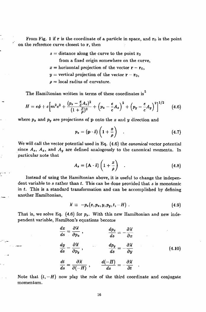
It is useful to use a coordinate system based on a closed planar reference curve. This reference curve is taken to be the closed trajectory of a .particle with some reference momentum po in the guiding magnetic field. The coordinate system (z, S, y) is similar to a cylindrical system, however, the radius of curvature may vary along the curve.

15

.

From Fig. 1 if r is the coordinate of a particle in space, and re is the point on the reference curve closest to r, then

s = distance along the curve to the point ro from a fixed origin somewhere on the curve,

x = horizontal projection of the vector r - ro, y = vertical projection of the vector r - rc, p = local radius of curvature.

‘The Hamiltonian written in terms of these coordinates is5

(P, - $&)2 (1 + gJ2 + (PZ - EAz)2 + (P, - ;Ay )‘I 1’2 (4.6)

P - where p, and p, are projections of p onto the x and y direction and -

p, = (p * SI) 1+ 5 ( )

. P km

-

We will call the vector potential used in Eq. (4.6) the canonical vector potential since A,, A,, and A, are defined analogously to the canonical momenta. In particular note that

. (4.8) _.__ _ - Instead of using the Hamiltonian above, it is useful to change the indepen-

dent variable to s rather than t. This can be done provided that s is monotonic in t. This is a standard transformation and can be accomplished by defining another Hamiltonian,

u - -ps(x,pz,wy,t,-H) . (4-g)

That is, we solve Eq. (4.6) for p,. With this new Hamiltonian and new independent variable, Hamilton’s equations become

_ ._ - - _ --

-

dx i3N -- ds - apz ’

dpz ax ds =-ii% -

dy a?/ 2. dpY _ dU -- ds - dp, ’

- - -- ds i3y

--

(4.10)

dt dU -= ds d(-H) ’

4-H) = aJ/ ds at *

Note that (t, -H) now play the role of the third coordinate and conjugate momentum.

16

4.3 THE LINEARIZED EQUATIONS OF MOTION i ,c- . . . .

. To be specific we will specialize to the case of no electric field and a constant magnetic field given by

By = -Be(s) + Bl(S) x + - - - B, = Bl(s)y+... .

(4.11)

The main bending field BO (s) is chosen so that a particle at the reference momentum po will bend with a local radius of curvature p(s). Thus, we set

Be(s) = E v(s) ’

(4.12)

Bl(s) in Eq. (4.11) is simply the gradient of the magnetic field. It is conventional and useful to scale the gradient to obtain the focusing function,

-

Kl(S) = s . (4.13)

Using Eqs. (4.12) and (4.13) the canonical vector potential which yields the above magnetic field is

- As=-~[;+(-+) ;+?I+... . (4.14)

_.~.._ _ The new Hamiltonian from Eq. (4.9) is

)/ = (-ps) = +! - ( )[ H2

1+; --J- m2c2 - pz - pi 1 112 . (4.15)

Since there is no time dependence, H is a constant of the motion which we call E ( the energy). In an actual accelerator the magnetic fields do change in time, and there are longitudinal electric fields to accelerate the particles. However, the acceleration process is slow and can be considered adiabatic for our purposes. In addition, the longitudinal electric fields cause longitudinal oscillations which are omitted here.

_ ._ -

To continue we expand the square root in Eq. (4.15) and substitute the vector potential from’Eq. (4.14) to obtain

- _ --

.- Jl= (PO-P$+Po : [($-+f+&$] +g+g+-- , (4.16) ,,

where p is the total kinetic momentum of the particle,

p = [E2/c2 - m2c2]1/2 , (4.17)

which may be somewhat different from the reference momentum. The expansion

17

of the square root is a good approximation provided that .-- . . . .

PZ,Y . I I - << 1,

P (4.18)

which is typically the case. From Hamilton’s equations and the Hamiltonian in Eq. (4.16) we find

dx px dpz -=- - = -po ds p ’ ds dy PY dpy _ -- ds=p ’ ds -POKIY .

(4.19)

In terms of x and y Eqs. (4.19) become

- PO&

y” + - p Y=o ,

(4.20)

where prime denotes differentiation with respect to s. Equations (4.20) yield the motion of particles near the reference orbit. Because Kl and p are periodically dependent on s with period C , the circumference, these equations are Hill’s equations.

5. LINEAR EQUATIONS WITH _._._ _ - PERIODIC COEFFICIENTS5

There have been many useful techniques developed for linear equations with periodic coefficients in the context of alternating gradient focusing for particle

.-- accelerators or storage rings. In this section we follow Ref. 5 to develop these, now standard, techniques in one dimension. The matrix approach is used ini- tially to understand stability and introduce the very important function p, the Courant-Snyder amplitude function. Next we find a canonical transformation which changes the Hamiltonian to that for a harmonic oscillator. Finally we discuss the adiabatic damping of bet&on oscillations with acceleration. In this section the discussion is restricted to the case of a particle with momentum equal to the design momentum1 Thus we find two uncoupled homogeneous differential _ _ _Y_ equations of the form - L.

- 2 + K(s)2 = 0 (54

which can be derived from the scaled Hamiltonian

H=;+ 2 . K(s)z2

(5.2)

-

z represents either horizontal or vertical displacement, and K satisfies the peri-

18

odicity relation ,c-

. K(s + C) = K(s) . (5.3)

Here C is the circumference of the equilibrium orbit.

In a circular accelerator or storage ring the magnetic “lattice” ideally consists of N identical sections or “unit cells”, so that K also satisfies the stronger periodicity relation

K(s + L) = K(s) ; L = C/N. (5.4

5.1 THE MATRIX APPROACH -

The solution of any linear second order differential equation of the form (5.1) is uniquely determined by the initial values of z and its derivative 2:

z(s) = az(so) + bz’(s0) , -

z’(s) = ci(s,) + dz’(so) , (5.5)

_._._ . - In matrix notation this can be written

-- Z(s) = [J =M(sIso)z(so)= [: :I [;(J . (5.6)

The matrix formulation is useful because it separates the properties of the general solution from those due to a specific initial condition. The matrix depends only on K(s) and the length of the interval s - so. In addition, the matrix for any interval made up of sub-intervals is just the product of the-matrices for the

_ ’ _-. sub-intervals, that is, -s---- L.

M(S2lSo) =qS%Isl)M(sllso) - (5.7)

C

It is important to note that the determinant of the matrix M is equal to unity, because Eq. (5.1) was derived from a Hamiltonian and thus does not contain any first-derivative (dissipative) terms.

19

For the case of constant K which corresponds locally to a harmonic oscillator ,z.- solution, the-matrix is

.

r cos f$ Km1j2 sin 4 1 M( SI so) =

-K’j2 sin C$J cos f$ J

,

where 4 = K1i2(s - SO). Wh en K is negative, this is sometimes written

cash + (-K)-‘1” sinh$

M= (-K)li2 sinh$ cash II, 1 ,

(5.8)

(5.9) -

where $ = (-K)li2 (s - se). Finally for an interval of length .! in which K = 0, Eq. (5.1) can be trivially integrated to yield

1 e

M= [ 1 .o 1’ (5.10) -

_._._ * c Perhaps the most important point is that for an interval in which K is piecewise constant the matrix for the total interval is the product of the appropriate matrices of the forms (5.8) to (5.10).

In the periodic systems considered here the matrices of particular importance are those which map the initial condition through an entire period. Let us abbreviate this one turn matrix as follows,

M(s) = M(s + LI s) . (5.11)

_ _T_

This is the matrix for passage through one period, starting from s. Due. to the periodicity of K the elements of M(s) must be periodic functions of s with period L. The matrix for passage through one revolution composed of N identical cells L- is

- M(s + NLI s) = [M(s)]~ .

Finally, the matrix for passage through k revolutions is [M(s)lNk .

In order for the motion to be stable all the elements of the matrix MNk must remain bounded as k increases indefinitely. To obtain the condition for

20

this, we consider the eigenvalues of the matrix M(s), that is, those numbers X i r-- for whichthe characteristic matrix equation i

. MZ=XZ (5.12)

possesses non-vanishing solutions. The eigenvalues are the solutions of the determinantal equation

Det(M - XI) = 0 , (5.13)

which yields the characteristic equation,

X2--(u+d)+l=O , (5.14)

- where we have made use of the fact that Det M = ad - bc = 1. Defining

cos~~~~rM=~(u+d) , (5.15)

the two solutions of (5.14) can be written

X=cosp-f i sinp=e*@. (5.16)

_...._ _ The quantity p is real if la + dl 5 2, and complex if la + dl > 2. c

Assuming that la + dl # 2, the matrix M may be written in a form which exhibits the eigenvalues explicitly. To do this define cosp by (5.15), and define a, A and 7 by

a-d=2a(s)sinp ,

b = p(s) sinp , (5.17)

c = -7(s) sinp .

The condition Det M = 1 becomes

_ . _zz_

P7 Y- a2 = 1 , _- (5.18)

.- and the matrix M can now be written

-

cosp + asinp psink

M= -7 sin p cosp - cusinp 1 = Icosp + Jsinp (5.19)

21

where I is the unit matrix, and ,c- . . . .

. aP J= [ 1 -7 --a

(5.20)

is a matrix with zero trace and unit determinant which satisfies

J2 =-I . (5.21)

It is important to note that the trace of M, and therefore p, is independent of the reference point s. From (5.7) we have

Mb2 + LI ~1) = M(s~)M(s~IsI) = M(4 sl)M(sl) , (5.22)

so that

-

M(s2) = M(s2 IsI)M(sI)[M(s~ 1 a)]-’ . (5.23)

Therefore M(q) and M( s2 ) are related by a similarity transformation, and thus have the same trace and eigenvalues. However, the matrix M(s) as a whole does depend on the reference point s. Thus the elements Q, ,B, 7 of the matrix J must be functions of s, periodic with period L.

_._._ . To examine stability simply recall that the eigenvalues of M(s) have the - form

X = efip .

Thus, the eigenvalues of M(s) k are given by

(5.24)

Ak = efikp . (5.25)

For stability the Xk must remain bounded as k --+ 00. This means that p must be real since in this case the eigenvalues have unit magnitude and the matrix elements of M(s) simply oscillate with increasing k. Recalling the definition of ~1 in Eq. (5.15), the motion is stable provided

Trace[M(s)] < 2 , (5.26)

- and is unstable if

Trace[M(s)] > 2 . (5.27)

-

Thus, to summarize, the matrix approach can be used to construct explicitly the periodic matrix elements a, 6, c and d. Once the one-turn matrix at a point

22

SO is known, its trace can be calculated. This yields CL, which can then be used ,cm to calculate &, 7 and ,B at the point so. The values of cy, 7 and p at other points

. can then be calculated oiu the similarity transformation in Eq. (5.23). In this case the matrix elements change but p remains fixed, and thus the change is entirely due to QI, 7 and p.

These parameters play a major role in determining the details of the motion. In particular, ,O determines the maximum local amplitude of transverse oscillations. This is demonstrated in the next section.

512 THE PHASE-AMPLITUDE FORM OF THE SOLUTION

The previous section suggests that we might consider a solution of the form

zl(s) = w(s)ei+(8) . (5.28)

Upon substitution into Eq. (5.1), ‘t I is straightforward to verify that if w and $J satisfy

- and

w”+Kw-l=(-j W3

(5.29)

+I=-$ , (5.30) _._._ . - then zr as defined by Eq. (5.28) is indeed a solution to Eq. (5.1). In addition

22(s) = w(s)e-i+(8) , (5.31)

is also a solution and zr and 22 are linearly independent. Since any solution of (5.1) can be written as a linear combination of zr and 22, we can write the matrix M( s2 I sr) in terms of zr. Using the form of the solution in Eq. (5.28) the matrix becomes

M(s2lsl) = _ _ _Y_ zcos 4 --w2w{ sin $ wrw2 sin-+

-1 - wrw;w2w; (5*32) - ----I Wl w2 sin+ - (2 - 2) cos$ $cos$ + irwisin(il

I

where $J stands for T+!J(s~) - +(sr), wr for W(Q), etc.

Consider for example the case where s2 - sr is just one period of K(s), i.e., s2 - sr = L. In this case the matrix M is identical with the matrix (5.19). If we

23

-_ require that W(S) b e a periodic function of S, then ~1 ‘- the forms-(5.l9)and (5.32) are identical provided that

. !+a) - ?+l) = P ,

w2=p ,

ww’=-(Y ,

which yields 1 + (ww’)2 1+ fX2

W2 =--.-..-x~*

P

= w2 and wi = wk, and

(5.33)

(5.34)

(5.35)

(5.36)

The above identifications are legitimate provided that we can show that p1/2 satisfies the differential Eq. (5.29) and that

p’ = -2cr . (5.37)

To prove this, consider the one-period matrix for the transformation from s + ds to s + L + ds. From Eq. (5.23) the matrix is given by

M(s + ds) = M(s + dsl s)M(s) [M(s + dsJ s)]-’ . (5.38)

However, from the differential equation in Eq. (5.1), it is easy to see that

1 ds - .- . - M( s + dsl s) = [ 1 -K(s) ds 1 ’ (5.39)

v Therefore, if we substitute (5.39) and (5.19) into (5.38) we find

[(KP -r)siv -2crsinp 1

M(s + ds) = M(s) +

J

ds. -2Ka sin p -(KP - 7) sinj.k

(5.40)

Inspecting the upper right matrix element, we see that (5.37) is indeed valid. In addition from the other matrix elements, we obtain -

_ _ _-. ._ --- 1+CY2 &‘+~~~~~-r=~p--

P (5.41)

.- and

7’ = 2Ka. (5.42)

-

Using (5.37) and (5.41) one can verify that p112 does indeed satisfy (5.29), and is thus a periodic solution of that equation. Therefore, Eqs. (5.34) and (5.35) are

24

justified. Combining Eqs. (5.30) and (5.33) we find the very important relation ,-- . . . .

. (5.43)

Equation (5.43) may be regarded as the definition of CL. It is consistent with the previous definition, (5.15), but is unambiguous; equation (5.15) only defines p modulo 27r.

Considering an accelerator of circumference C = NL with N identical unit cells, the phase change per revolution is Np. It is also useful to define

s+c Np 1 ds’ y=-=-

/- 2Tr 27r p ’ S

(5.44) -

-

which is the number of betatron oscillation wavelengths in one revolution. Al- ternatively, Y is the frequency of betatron oscillations measured in units of the revolution frequency; here we refer to ZJ simply as the frequency or tune of betatron oscillations.

Using the previous results zr and z2 may be written in the following useful form,

_._._ . - zi = ~112(s)e*iv~(s) , (5.45)

where

The function 4(s) increases by 27r every revolution. The general solution of (5.1) can therefore be written

z(s) = .p112 c+5w + 61 , (5.46)

where a and 6 are arbitrary constants. This is a pseudo-harmonic osciilation with varying amplitude ,81i2 (s) and varying instantaneous wavelength

G _ _ _Y_ ~-

x =&3(s) . (5.47)

Note again that the m&mum amplitude at a fixed position se on successive revolutions is simply proportional to ,B(so)‘/~. For this reason p(s) is called the Courant-Snyder amplitude junction.

25

5-3 ACTION-ANGLE VARIABLES ,x- . . L.

. Now let us assume that we have explicitly calculated p(s) and 4(s). Then it is useful to construct action-angle variables for this problem in a way completely analogous to the harmonic oscillator in Section 3.2. To do this first write the scaled Hamiltonian for betatron oscillations from Eq. (5.2),

K(s)z2 2 *

Next write the solution for both the position and momentum,

z = a/?1/2 cos(uqqs) + 6)

(5.48)

p = -,p-112 [ sin(d+) + 6) - $os(u~(s) + 6)]

(5.49) .

The momentum equation is obtained by simply differentiating the equation for z.

- Using the solution above as a guide let us search for a canonical transformation of the form

_._._ . 2 = a (J)@12 cos $b -

p = -a( J)p-‘/2 sin $ - f cos II, 1 (5.50)

where J and $ are the new momentum and coordinate respectively. We will use a generating function of the first type; therefore, we need the old momenta p in terms of the new and old coordinates. Combining the two equations in (5.50) yields

p=-- i (tan$-c) . _ -(5.51)

-

--- Therefore, Eq. (3.10) for the generating function can be- integrated to yield

Fl(z,$) =-$ [t-$-c] . (5.52)

-

C

Solving for the new momenta in terms of the old coordinates and momenta,

26

L we find ,c-

J= $[z2+ (p&~)‘]

and the complete set of transformation equations becomes

p= -dm(sin$-Tcos$) ,

Hl = H + aF+s = J/P(s) *

(5.53)

(5.54)

The differential relations for ,O in Eq. (5.41) have been used to simplify the new Hamiltonian.

In these new coordinates the solution of the equations of motion is

J = constant

- Icl(s) = ti(o) + i’ & - 0

(5.55)

_._._ . - Note that in the process we have explicitly constructed an invariant, J.

Equation (5.53) for the invariant is the equation of an ellipse in phase space which rotates periodically in s. If a particle has initial conditions which begin

._ on some ellipse given by Jo, then the coordinates and momentum of that particle always stay on that ellipse.

Looking at it in another way, consider a single particle traversing the periodic focusing structure and plot its position and momentum in phase space each time it passes s = so. Then, the locus of those points is an ellipse in phase space. At points other than se, the ellipse so generated evolves according to Eq. (5.53). If we extend phase space to include the independent variable s, we find a 3-

. dimensional extended’phase space and the motion is confined to the 2-torus ._ Tz _ -&fined in Eq. (5.53), L.

The invariant J is simply related to the area enclosed by the ellipse, -

Area enclosed = 27rJ . (5.56)

-

In accelerator and storage ring terminology there is a quantity called the emit-

tance which is closely related to this invariant. The emittance, however, is a

27

property of a distribution of particles, not a single particle. Consider a Gaussian ‘Cm distribution in amplitude. Then the (rms) emittance, E, is given by

(h3)2 = P(s) E - (5.57)

In terms of the action variable, J, this can be rewritten

E = (J) (5.58)

where the bracket indicates an average over the distribution in J.

Finally note that the form of the new Hamiltonian is not precisely that of a harmonic oscillator in that the phase does not advance uniformly. This of course causes no difficulty in that both cases are trivial to solve. However, it is possible to perform another canonical transformation to coordinates which have a uniformly advancing phase. This is accomplished with the canonical transformation:

-

S

F2(+,J1,s) = J1 F-17 [ 1 +lclJl , 0 . .

_._._ . dl++zymj~, - 0

J1=J,

--- Hl=FJ+ J1 .

(5.59)

In these new coordinates the oscillating part of the phase advance has been extracted leaving only the average phase advance. Either these coordinates or the previous set can be used in the section on canonical perturbation theory; however, we will use the second set since no reference is made to a specific problem. In the later sections we will use the first set (J, $) since this simplifies the notation in spite of the fact that one must integrate to obtain the phase .-A?- L. advance.

-

C

28

5.4 ADIABATIC DAMPING ,-- . . L.

. In the previous sections the case of a constant momentum equal to the design momentum po was considered. From a scaled Hamiltonian and the known solutions the invariant J was calculated. In this section we consider the case of slow acceleration so that the momentum p and the magnetic fields (oc PO) slowly increase together with p = po. In actual accelerators the acceleration time is much longer than either the revolution period or the betatron period. However, although this slow change does not affect the single particle dynamics, it does lead to the adiabatic damping of the action J and thus the emittance of a beam of particles.

To see this effect we return to a Hamiltonian of the form in Eq. (4.16),

N = g + PoKf)Z2 . (5.60)

where once again z refers to either x or y and K(s) refers to the appropriate focusing function. As in the previous section we can perform the change to action angle variables. The generating function of the transformation (z, pz) I+ (W, $) is

Fl(z,q$) = -EC 2P (4 [

tan+- $i 1 ,

which leads to the transformation equations _ .- . - z = @qi&osti ,

p=-dw sin+-ccos$ (

,

HI = U + dFl/i3s = W//~(S) .

(5.61)

(5.62)

Here, again, the phase advances as in the previous section; however, the invariant is given by

wA![z2+(!!&~)2]. _ (5.63)

_ ’ _Y. From Hamilton’s equations

L. PZ dz --=-xz’ p. ds - ’

(5.64) -

- _ and therefore from Eqs. (5.53) and (5.63), W and J are related by

W =poJ. (5.65)

-

Now consider the adiabatic variation of po. In this case the action W is an

29

I adiabatic invariant and is very nearly constant; therefore,

. . . .

. J=%pi’. PO

(5.66)

This is called adiabatic damping. It means that as a particle beam is accelerated in a circular (or linear) accelerator, the emittance is inversely proportional to the momentum. Therefore, from Eq. (5.62) the transverse beam size varies as . 112 z=,q !T! [ 1 . P

(5.67)

Due to this variation it is useful to define an auxiliary quantity, the invariant or normalized emittance, which is constant,

&N = P7r . (5.68)

This quantity is proportional to the area in phase space (z,pz) occupied by the beam distribution.

The damping discussed does not apply to electrons in circular accelerators or storage rings since the effect is small compared to radiation damping. For a discussion of radiation damping and quantum excitation in circular accelerators see Refs. 6 and 7 and references therein.

5.5 THE ADIABATIC INVARIANCE OF THE ACTION _ .- . - It is straightforward to show that W, the action for betatron oscillations

discussed in the previous section, is an adiabatic invariant. To do this we resort again to the very powerful technique of canonical transformations. Since we already have the parametric dependence of the transformation to action-angle variables on pot it is now only necessary to allow that po depend upon s. In this case the transformation to the action-angle variables discussed in Section 5.4 is still valid; however, the new Hamiltonian is no longer independent of $ the angle variable. In this case the transformation to the new Hamiltonian from Eq. (5.62) becomes

_ _-. Hl~=H+g

izr- W . = - - &TV [sin2$ - /3’(s) cos2 $1 ,

P(s) 2Po -

where the rate of change of the momentum is

I - dP0 Po=-jy. (5.70)

-

Equation (5.69) is the Hamiltonian which describes betatron oscillations in the

30

,c- presence of acceleration. The phase and action variables evolve according to

. dlCI 1 - - - pb [sin2+ - p’(s) cos2 $J] d$ - P(s) 2Po

-= ds --$$W[COS 2$J + p’(s) cos 27) sin 2+] .

(5.71)

We would now like to show that the variation of W is quite small for small pb even if the total change of momentum is quite large. We do this by inspecting the differential equations in Eq. (5.71). For the purpose of this demonstration it is useful but not essential to smooth the betatron oscillations. This is done by setting p’ = 0 and p(s) = constant = p which yields

dW pb -=-

ds PO (4 wcos2+ .

(5.72)

To zeroeth order the phase variation is simply unperturbed. Substituting this approximate solution of the phase equation into the differential equation for the act ion yields

- dW -E ds &w cos(2s/P + $0) * (5.73)

_._._ . -

By inspecting Eq. (5.73) f or small pb and thus slow variation of PO, it is easy to see that W is nearly constant. This is due to the rapid oscillations of the right hand side. If PO(S) varies little in one betatron period, then the variation of W

-- averages out over one betatron oscillation. For finite changes in PO(S) there is a small non-adiabatic contribution.

This can be estimated by integrating Eq. (5.73) over the entire acceleration cycle. To do this we assume a linear increase of the momentum and the magnetic fields which bend and focus the beam, that is,

PO(S) =Pi+P’s * (5.74)

_ ._ -. Integrating Eq. (5.73) is straightforward to show that for small p’ the change - -- -+rraction is limited by 2.

- - _ pii+ (Fig) (pizip) ’ (5.75)

-

C

where Ap is the total change in momentum. Note that the variation in W is small even for large Ap provided that the change in momentum in one betatron wavelength (27rpp’) is small compared to the initial momentum.

31

6. THE NONLINEAR TERMS ,c- . 6.1 THE SOURCES OF NONLINEARITY AND CHROMATICITY

The nonlinear terms that have so far been neglected come from several sources. The so-called geometric terms arise from terms in the longitudinal vector potential which are higher than quadratic. These arise from both deliberate and inadvertent nonlinear magnetic fields. In addition, there are higher-order terms in the transverse components of the vector potential which are necessary to satisfy Maxwell’s equations. There are also kinematic terms which come from the expansion of the square root in Eq. (4.15). F’ mally, in colliding beam storage rings there is the beam-beam force. A particle from one beam feels the electric and magnetic fields due to the collection of all the particles in the opposing beam. The beam-beam force is typically very strong, quite nonlinear, and of a different character than the others mentioned; therefore, it is usually treated separately. For useful reviews of the beam-beam effect see Refs. 8 and 9.

Aside from the beam-beam force, a dominant source of nonlinearity comes from the deliberate use of sextupoles to cure chromatic effects in storage rings. Before discussing the deleterious effects of sextupoles on the homogeneous equations, it is first useful to motivate their inclusion in the first place.

Let us first examine the Hamiltonian for betatron oscillations in Eq. (4.16). Since in all cases considered here p varies only adiabatically, it is first useful to scale the Hamiltonian with p to make it dimensionless. Defining the quantity

_._._ . - A&-PO

P ’ (6.1)

._ the effective Hamiltonian becomes

$=-Af+(l-A) [(-+I) ;+KI;] +$+$+- (6.2)

which is simply the Hamiltonian in Eq. (4.16) scaled appropriately. Note that in these new variables the canonical momenta are simply equal to the slopes.dx/ds and dy/ds as is easily.verified through Hamilton’s equations. -The quantity A

_ _ _Y_ measures the deviation of the actual momentum from the momentum on the - ._ ;zr reIerence orbit. It is clear from the Hamiltonian in Eq. (6.2) that ‘the solutions

- of the linear equations of motion will depend on A as a parameter. Since all particle beams have a finite spread in momentum, this ‘chromatic’ dependence is undesirable. In addition, there is a collective instability (the head-tail effect) which is enhanced by these chromatic effects; thus, it is necessary to provide some chromatic correction.

-

-

C

32

6.2 SEXTUPOLES FOR CHROMATIC CORRECTION

To see the effects of sextupoles we must first include them in the Hamilto- nian. The vector potential for a sextupole magnet is

eA,/c = poy(x3 - 3xy2) . (6.3)

In terms of the magnetic field

S(s) = &$$ . (6.4

S(s) is a periodic function of s which is typically piecewise constant in the regions where the correction sextupoles are placed and zero elsewhere. If S(s) comes from errors in magnetic field, then the strongest contribution is usually in the bending magnets which are typically pure dipole magnets.

The new Hamiltonian including sextupoles is

- ti = $+$-+(1-A) X2

-KzT +Kl$ +(14)~(~~-3~y~) (6.5) 1 _._._ . where we have defined -

--. in order to simplify the notation. Using Hamilton’s equations, the differential equations for the motion are

x” - (1 - A)KZx + (1 - A);(x2 - y2) = A P (6.7)

y” + (1 - A)Kry - (1 - A)Sxy = 0 .

_ _ -1. The equations above ‘may look slightly different from and somewhat simpler - ._ &an others in the literature. The difference arises due to the definition of A

chosen here. -

- _ At this point it is necessary to calculate the periodic solution to Eq. (6.7)

above. This will give us the closed orbit for an off momentum particle in the full nonlinear field. By inspection we can see that once again the vertical closed orbit simply vanishes. In the horizontal direction it is conventional and useful to introduce the dispersion function D. If we let the periodic solution be xE(s),

-

. .

33

then I

D(s) = xE(s)/A j (64

where, of course, D(s) is a periodic function of s. Writing the equation for the horizontal dispersion we find

D” - (1 - A)K,D + A(1 - A&I2 = f . (6.9)

D(s) is the periodic solution to Eq. (6.9). With this definition, D depends upon A; however, since A is typically quite small, the dependence is weak. The more familiar linear dispersion function Do is obtained by setting A and S to zero in Eq. (6.9). D can be thought of as the exact dispersion function for the Hamiltonian in Eq. (6.5).

Now we would like to perform a canonical transformation to place the periodic orbit just calculated at the center of phase space. This transformation (x,pZ) H (xp,pp) can be accomplished with the generating function

fib, 193) = (x - AD(s))(p, + AD’(s)) , (6.10)

which yields the transformation equations

. ..-. . -

x =‘xp + AD(s)

pz = pp + AD’(s) .ri, = ?? + 8F2/& .

(6.11)

Substituting using the Hamiltonian in Eq. (6.5) yields the new Hamiltonian

-u

$=~+~-KzT+K~~+~(x~-3xpy2) x;

+ A -[

(SD(s) x; + Kz)z - (SD(s) + 4); - f(x; - 3xpy2) 1 _ A2 sD(s)

--+$ - Y2) -

(6.12)

_ ._ -. Examining the linear chromatic terms, we find that sextupoles contribute to the - ._ &near differential equations at points-where the dispersion D is nonzero. Thus,

by adjusting S(s) one can cancel many of the chromatic effects. In particular, - one can cancel the linear variation of the tune with momentum.

Unfortunately, in the process of cancelling the chromatic effects, we add nonlinear terms to the equations of motion. To begin the study of the effects of these nonlinear terms on the motion, in the next section we discuss canonical perturbation theory.

-

C

34

7. CANONICAL PERTURBATION THEORY ,c- . In this section we seek a method to study nonlinear effects perturbatively.

We do this by attempting to find a canonical transformation which makes the new Hamiltonian a function of the new momenta alone. This is just the approach which yields the Hamiltonian-Jacobi equation; however, in perturbation theory the new Hamiltonian may depend upon the coordinates and time in higher order.

7.1 THE EQUATION FOR THE GENERATING FUNCTION

Suppose that the problem can be described by a Hamiltonian

H = Ho(J) + V(@, J$) P-1)

where H has been written in terms of action-angle variables of the unperturbed - problem and bold face characters denote d-dimensional vectors. The unper-

turbed Hamiltonian Ho includes nonlinear terms which depend only on J; thus, the unperturbed tune may depend upon amplitude. In the absence of the perturbation, the action variables are invariant and the motion is confined to a (d + l)-dimensional torus in the extended phase space (J, a, 0). In the following we-look for the distortions of this torus due to the nonlinear perturbation.

- Note that in this section we have scaled the independent variable from s to 8 so that the Hamiltonian is 27r periodic in both the angle variables Q and the independent variable 0. In particular, the nonlinear perturbing term V(Q, J, 0)

_._._ . - is a periodic function of B and Q and has zero average with respect to them, i.e.,

2r 2r

/ J de d@ V(Q, J,e) = 0 . .- (7.2)

0 0

If V has a nonzero average, the average value of V can be absorbed into Ho(J).

Consider a canonical transformation (J, 4D) H (Jl, @ I) with a generating function of the following form:

F@,Jl$) = a-J1 + G(@,Jl,b’) . (7.3) _ _ ._ - The above transformation is close to,the identity provided that G is small. The - _ s-

new coordinates and ‘Hamiltonian are given by -

@I=@ + GJ, - _ J=J1 + G9 (7.4

HI = H + Go

-

where the subscripts indicate partial differentiation.

35

The new Hamiltonian after substituting the transformed variables is i ,c-

. HI = Ho(JI+G~P)+V(@,JI+G~,O)+G~ . (7.5)

Note that we have substituted so that the Hamiltonian is a function of the same variables as G, the old coordinates and the new momenta. Eventually we must complete the substitution; however, for the moment it is more convenient to work with the mixed variables. Equation (7.5) can be rewritten in the interesting form

HI = Ho(Jl) + [Ho(Jl + GB) - Ho(Jl) - I . GQT] + [V&J1 + Gd’) - V(@,Jl$)] + y(J1) . GB + G + V(@, Jd) ,

(7.6)

where By is the vector frequency as a function of amplitude of the unperturbed problem,

-

aHo v(J) = aJ . (7.7)

If we can find a solution to the equation - -

v(J1) - Ga + Ge + V(@, J1,8) = 0 , V-8)

_._._ . G will be a quantity of order V. All other parts of the new Hamiltonian are - either independent of the coordinates and time or are of order V2. To see this

more easily we can expand for small G to obtain

__ HI = Ho(Jl)+Y(Jl).GO+GB+V(~,J1,e)+[G,.y,,.G~/2+VJ,,G~]+... . (7.9)

7.2 THE SOLUTION FOR THE GENERATING FUNCTION

Since we are looking for the distortions of the invariant torus, we must find the periodic solution to Eq. (7.8); h owever, in order for a periodic solution to exist, the average value of V must vanish. This was anticipated by our earlier

.-=._ requirement in Eq. (7.2). -- - L. Since both V and G are periodic functions of @, they can be Fourier ana- -

lyzed, - _ V(@, J1, 6) = c um(J1, B)eim‘@

G(@,Jl,O) = Egm(JI,8)eim’@ . (7.10)

m

36

Then the equation to be solved for G becomes ,c-

. im.v(Jr)+& gm=-um , 1 (7.11)

which has the periodic solution

e+27r i

9 m = 2sin(7rm s 21) s eim’p(e’-e-r) um (J 1, 6’) de’ . (7.12)

8

Finally, the full expression for G is given by

8+2r

G’1 i m 2 sin(7rm . v) J

eim.[@+v(e’-e-T)l urn ( J1 , 0’) &I’ . (7.13) 6

Sometimes it is desirable to make use of the fact that V is a periodic function of 8 to expand it as a ‘double’ Fourier series

- V = c um,(Jl)ei(m’a-ne) . m,n

(7.14)

..-._ . This leads to an alternative expression for the generating function in Eq. (7.13), -

G=i c umn( Jl)ei(m’*-ne)

. m-v-n

(7.15) man

7.3 THE NEW HAMILTONIAN AND THE AMPLITUDE DEPENDENCE OF THE TUNE

Recall that our original purpose was to transform the Hamiltonian into a form which is approximately independent of the coordinates and the time. The new Hamiltonian in Eq. (7.9) is now given by

_ ._ - - - -- HI = ITo + [VJ, -%a + Ga - vJ1 - G&2 -t - - -]

- Ho(J1) + V’(J1, QTd) . (7.16)

-

- _ The remaining nonlinear term can be separated into a part which depends only on the new action variable and into another part which involves Jr, @r and 8 but which has zero average value. This oscillatory term is the object of the next canonical transformation, whereas the term which is a function of the new

37

i action variable Jr leads to a change of frequencies with amplitude. The latter ‘%- term is given- by

2r 2n

JJ de da [vJ1 -G~+G~-'J1 - G@/2++ . (7.17)

0 0

Separating the average value, the new Hamiltonian can be written

HI = [Ho(Jl)+ (V'(Jl)> ] + [ V'- (V') ] = - Hol(J1) f Vl(@l, Jldq

(7.18)

and the new frequency becomes -

aHo W’> vl(Jl) = aJ = v(Jl)+ dJ . 1 1

(7.19)

-

Note that if we examine the new perturbing term VI, it is second order in the strength of the perturbation. In addition it is higher order in Jr. If the original perturbation has a lowest-order contribution of order Jf, then the new term is of order J1(2*-1). Therefore, for sufliciently small J1 , we can neglect VI. If this is done, we have a new Hamiltonian which depends only upon the new momenta.

_._._ . Therefore, these new momenta are (approximate) constants of the motion, and - from Eq. (7.4) for J(@, Jr,8) th e motion is restricted to a (d + 1)-dimensional

torus in phase space.

-u To proceed to higher order in perturbation theory there are two approaches.

In the first approach we return to the generating function in Eq. (7.3) and express it as a power series in the strength of the perturbation. Then upon substitution into the Hamiltonian in Eq. (7.5), we obtain a hierarchy of equations as we cancel the perturbing terms order by order. In this approach if E is the strength of the perturbing term, after the nth term of order ~(~+l).

step we are left with a perturbing

In the second approach we begin where we left off and make successive _ _ _Y_ canonical transformations which are formally identical to the first one. This

- - -method is called superconvergent perturbation theory and was first introduced in this context by Kolmogorov in his proof of the KAM theorem. It is called - superconvergent because on the nth step the remaining perturbing term is of order c2”. Despite the name, however, the method need not converge! If the procedure does converge, then it does so much faster than the first method.

C

Unfortunately these methods do not always work. Everything would be fine if G were always small; however, a quick inspection of Eq. (7.13) shows that

38

c this is not the case for arbitrary V. There are resonances whenever ,=-. . . . .

. m . u = integers . (7.20)

This happens because we have required periodic solutions to the equation for G. It is straightforward to see that if the resonance condition is satisfied, there are no periodic solutions to Eq. (7.11). In fact the amplitude of the solution grows linearly in 8.

.Thus, in the neighborhood of a resonance one must abandon perturbation theory at least insofar as it applies to the resonance. We can continue to use perturbation theory for the non-resonant terms, but we must isolate the resonant term for special treatment. Before beginning the study of isolated resonances, it is first useful to apply perturbation theory to a few simple cases.

8. LINEAR PERTURBATIONS

It is interesting and useful to apply the canonical perturbation theory developed in the previous section to linear perturbations. In these cases we can

- solve the perturbed problems exactly; however, it is quite useful to have analytic formulae which describe the effect of a small perturbation. First consider the perturbation of the quadrupole gradient in one degree of freedom.

_._._ . - 8.1 QUADRUPOLE GRADIENT PERTURBATION

In this case, the Hamiltonian we consider is

H _ p2 ; K(s)z2 ; k(s)z2 , 2 2 2 (84

where k(s), the coefficient of the linear perturbation, is considered small. The transformation to the action-angle variables of the unperturbed linear problem yields

If' = &) + Jk!y [1+cos(2qs)] . (8.2) -

Before proceeding it is necessary to include the average part of the perturbation in HO,

-

Ho = J [l/P(s) + +)P(s)/2] . (8.3)

This yields the shift of the phase advance to first order in the strength of the

39

perturbation, i ,---.

. 40(s) - 5qs) = ti(o) + k(s’)p(s’)ds’ . (8.4

The tune shift due to this additional phase advance is thus given by

c

AV = -& 1 k(s’)P(s’)ds’ , 0

(8.5)

where C is the circumference.

Eq. (8.5) above is the well known formula for the tune shift due to a small quadrupole perturbation. In canonical perturbation theory it is obtained simply by averaging the Hamiltonian to obtain Ho before proceeding to the first step of perturbation theory.

-

To calculate the first order distortions of the invariant curves it is only necessary to use the formula for the generating function in Eq. (7.13) to obtain

- s+c

G= -Jl 4 sin(27rrv) J

k(s’)P(s’) sin2(4 + $(s’) - $(s) - 7~) ds’ , (8.6) -. .- . 8

where u is the tune which includes the shift in Eq. (8.5). Note that the phase advance $J(s) from Eq. (8.4) appears in Eq. (8.6) rather than uB as in Eq.

-- (7.13). The approximate invariant curves are given by

J = JI + G&h JI,s) (8-V

with

51 = constant + O(k2) . (8.8) 4

From Eq. (8.6) we have explicitly ~-

s+c

J=Jl- Jl 2 sin(27rrv) /

k(s’)p(s’) cos 2($ + $(s’) - 9(s) - TV) ds’ . (8.9)

In standard accelerator physics literature one usually finds the distortions of the p function calculated rather than the invariant curves. This is simply related

40

to the variation in amplitude of the invariant curve at 4 = 0. Identifying the i ‘%-- new beta-function /3r (s), we find

. 5+C

A(s) -Do(s) = -1

PO (4 2 sin(27rrv) J k(s’)po(s’) cos 2($(s’) - $(s) - TV) ds’ . (8.10)

8

This form is somewhat different than usual in that it is the perturbed tune which appears in the formula.

8.2 WEAK LINEAR COUPLING

It is also interesting to apply canonical perturbation theory to the case of - weak linear coupling. The perturbed Hamiltonian is given by

H = 2 + f$ _ K&)x2 + Kl(s)Y2 + M(s)xy , 2 2 2

where M[s) is the skew focusing function defined by

- M(s) = ;$ .

(8.11)

(8.12)

_..._ . - In this case the transformation to the action-angle variables of the unperturbed

linear problem yields

Jl 52 -a.azs - -

H1 = h(s) + P2(s) + ~M(~)(PI~)“~(JI J2)li2 cos(&) cos(~,) . (8.13)

Now if we treat the last term above as a perturbation, we can use the perturbation theory developed previously.

From Eq. (7.13) the generating function in this case is

_ ._ - - --J2= -(11’2)1’2

2sin7r(y + V2)’ S ‘)[p ( ‘jJ? ( ‘)]‘/” sin Q (~$1 952. s s’)ds’ 1s 2s + 3 ,,

8 - (8.14)

- _ (1112)“2 - 2 sin 7r(yr - ~2)

d+cM( ‘)[/3 ( ‘)p ( ‘)]li2 sin \E-(41 ~$2 s s’)ds’ J

S 1s 2s , , , .

5

where the subscripts 1 and 2 refer to x and y, 11 and I2 are the new action

C

41

variables, and the phase factors in the integral are given by i ,---.

. w?M2d) = (41 + vh(s’) - @l(S) - w) f (952 + $2(s’)

where

’ ds’ hd4 = J p1 2(s,) *

0 ’

$5 (4

To calculate the invariant surfaces we simply use Eq. (7.4) to obtain

JI = 11 + G&ih,42J1,12,~)

J2 = 12 + G&h$2J1,12,s) ,

where 11 and 12 are constant.

(8.17)

-

In this case the distorted invariant surface is a 3-torus in the extended 5- dimensional phase space. If we make a surface of section at some se, then we remain with a 2-torus in 4-dimensional phase space. In the uncoupled case this torus is simply the direct product of the two ellipses from the horizontal and ver-tical phase spaces; however, in the case of coupling this is no longer true. There are at least two different ways to view the invariant surface. One can make another surface of section, say at ~$2 = ~$0, and view the resulting curve in (51, ~$1) phase space. Alternatively, one can project the surface onto a three dimensional subspace, (41 , 42, 51) or (&,r$z, 52). If we examine Eq. (8.17), we find that in these 3-dimensional subspaces the invariant surface remains a 2-torus. This surface can be viewed in perspective in each of the subspaces mentioned above. This latter method will be discussed in detail in Section 11.2.

-- Finally, in the linear coupling case, it is possible to return to the Hamilto- nian in Eq. (8.11) to find the eigenvectors which decompose the torus into the direct product of two circles by directly solving the linear differential equations. However, these do not project as simple curves in the original phase spaces.

42

9. A SEXTUPOLE PERTURBATION ,---- IN ONE DEGREE OF FREEDOM .

-

_._._

-

-u

_ ._ -.

-

In this section we apply perturbation theory to a sextupole perturbation in one degree of freedom. Since there are also coupling terms in the Hamiltonian in Eq. (6.12), one should actually treat the problem in two degrees of freedom. However, for the sake of brevity, we treat only one degree of freedom here; the extension to two degrees of freedom is quite straightforward by following the previous section.

From Eq. (6.12) we consider the non-chromatic part of the Hamiltonian for horizontal motion,

H = $I’ + K(s)z2) + yz3 . (94 Recall that S(s) is periodic with period C (the circumference) but may have stronger periodicity imposed by design. Transforming to the action-angle variables introduced in Eq. (3.19) we obtain the new Hamiltonian

H = J//3(s) + J”S( S )(Jp)3/2

= J/P(s) + $4, J,s)

cos3 r$

.

From Eq. (9.2) the perturbing term is

V(4, J,s) = &S(s)(JP(s))3/2[cos34 + 3~0~4 ,

P-2)

(g-3)

and using Eq. (7.13) the generating function is

G = - ${ 4siiau ~cds’S(s’),,s’)3~2 sin[4 + +(sI) - $(s) - zv] S

s+c 1

+ 12 sin 31rv / ds’S(s’)p(s’)3/2 sin3[+ + +(s’) - $J(s) - w]} .

S

(9.4 Note that since the phase of betatron motion does not advance uniformly like

X-harmonic oscillatorj the factor of u# in Eq. (7.13) is replaced in Eq. (9.4) by t)(s) where

-

Next we can evaluate the average of the new perturbing term from Eq.

43

(7.17). VJ, and G# are given by i ,c- . . . .

. VJ, = --&s(s)(Jl)1/2 p(s)3/2 [cm 34 + 3 cos $61

G, = -${ 4siiTv ~cds’S(,,,,,,/2 cos[d + $(s’) - t+b(s) - TV] s

(g.6)

s+c 1

+ 4 sin 37~ J

ds’S(s’)p(s’)3/2 cos 3[cj + $(s’) -

S

First we average over 4 to get rid of the cross term to obtain

ti(s) - 4) -

and then average over s

c

(VJ, G4) = - &

s+c

/ dsp(s)3~2S(s) J p(s’)3/2S(s’)ds’

-

x

{

3co:(rL(s’) - ?/J(s) - A) + cos3($(s’) - T+qs) - w) sin 7r~ sin 3~

.

P-7) If the actual distribution of sextupoles is known, the integral in Eq. (9.7) can be evaluated. If we drop the fluctuating term, the new Hamiltonian is given by

_._._ . -

The new tune is then turn

HI = J@(s) + (G+ VJ,) +‘-- . (9.8)

obtained by integrating the phase advance through one

0 ” v1(J1)=& - /( pt, + a-71

a(G,vJ~) ds

= y I ‘c a(G,vJ,)

> . (9.9)

27r dJ,

Since the additional term in the new Hamiltonian in Eq. (9.8) is of order J2, the tune in Eq. (9.9) varies linearly with J. This is similar to the first-order effect of

_ ._ - an octupole perturbation (- x4 ); therefore, a sextupole perturbation in second - - mer produces an o&pole-like nonlinear frequency shift with amplitude.

- Finally, the approximate invariant torus is given by

J = Jl + G~(Jd,s) , (9.10)

with 51 = constant. As the tune approaches n/3 the phase space curves obtained at some surface of section s = SO develop the characteristic 3’d harmonic

44

-

distortion of the third integer resonance. However, when the tune is too close ,Gs to a third-integer resonance, G is not small and perturbation theory is not ap-

. propriate. In the next sections we confront this problem for general nonlinear resonances.

10. AN ISOLATED RESONANCE IN ONE DEGREE OF FREEDOM

In Section 7 we discovered that there were resonances whenever

rn-v=n. (10.1)

Perturbation theory is not the appropriate method for studying the behavior - in the neighborhood of such a resonance. In this section we study an isolated

nonlinear resonance in one degree of freedom in detail, that is, a Z-dimensional phase space with a ‘time’ dependent Hamiltonian. We suppose that we are close to a resonance and that all other nonresonant terms in the Hamiltonian can be neglected. Thus, we are left with the truncated Hamiltonian,

- HT = UJ + a(J) + f(J)cos(mqS - d) . (10.2)

Note that we have separated Ho into a linear and nonlinear part, and that f(J)

_._._ . is taken to be positive in the region of interest. -

This problem can be solved exactly by using a canonical transformation to a rotating system in phase space. The generating function for the transformation (JA) H (Jdl) is

&(A JI) = (4 - nfl/m) Jl , (10.3)

which yields the transformation equations

41 = d - ?-d/m , J1 = J . (10.4)

The new Hamiltonian is then given by

_ ._ - HI = HT - y/m Jl = 6 Jl t, a( Jl) + I cos m$l , - (10.5)

- where

6=v-n/m . (10.6)

-

The Hamiltonian has been cast in a form explicitly independent of the ‘time’ variable 8; thus, it is a constant of the motion.

45

10.1 FIXED POINTS i ,c- . . L.

In the phase space (41, J1) we can find a set of points where the trajectories . are stationary. These fized points can be obtained by the conditions

aH1 o dH1 aJ,= ) -=o ,

%Jl (10.7)

which yield sin rn& = 0

6+cr’(J1)+I’(J1)cosm~l =O ,

where the prime above indicates differentiation with respect to J 1.

_..._ -

I I I I I I I I I I I

/2rp$;,;;, i/ /*

y ‘#/’ I

/ !’

\I ‘s8” \ l \‘\

:

i I ‘!Y\

i

\

i

f i

;<111:;

‘\

i

\ 1

i 1 I

1 \

i

J \i )

J

tk:<;&Tzz&y

c--N .- *----‘/ ‘-V.-C SFP

I I I I I I I I I I I

(10.8)

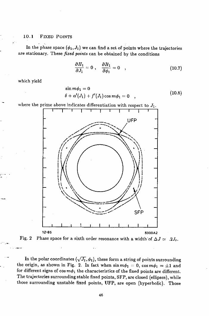
12-85 5300A2

Fig. 2 Phase space for- a sixth order resonance with a width-of A J N .2 Jr.

- In the polar coordinates (a, $I), th ese form a string of points surrounding - _ the origin, as shown in Fig. 2. In fact when sin rn& = 0, cos rn& = &l and

for different signs of cos mr,+i the characteristics of the fixed points are different. The trajectories surrounding stable fixed points, SFP, are closed (ellipses), while those surrounding unstable fixed points, UFP, are open (hyperbolic). Those

46

fixed points where cos rn& = -1 (+l) ‘; has a minimum (maximum) there.

are stable (unstable) since the potential

. Suppose we define Jr as that amplitude which yields an oscillation frequency at resonance, i.e.,

u + CY’( Jr) = n/m , (10.9)

then Eq. (10.8) becomes

a’( JI) - a’( Jr) + f’( JI) cos rnr$l = 0 (10.10)

or expanding for J1 close to Jr

(JI -Jr) = -$$cosm& . (10.11) r

- Therefore, provided that f’/ Q” is positive, the amplitude of the UFP is slightly less than Jr while the amplitude of the SFP is slightly larger than Jr.

10.2 RESONANCE ISLAND WIDTH

-The boundaries of the stable islands shown in Fig. 2 are formed by curves - joining the unstable fixed points. These curves are separatrices and their equa-

tion can be easily found by the fact that the new Hamiltonian HI is a constant on the curve.

_...._ . - From Eqs. (10.5) and (10.8), we have

6-h + I + f( Jl) ~0s wh = 6 Ju + cr(J,) + f( J,) , (10.12)

where J,, is the action at the unstable fixed point. Expanding for J close to Ju and recalling that Jr N Ju, we find that on the separatrix

(J - Ju)2 11 U(J,)(l - coswb) a”(J,) ’

From Eq. (10.13) we find the maximum separation or island width

(10.13)

_ ._ - - _ ;-*- (10.14)

- where a”(Jr) has been assumed positive for simplicity. Keep in mind that this is only valid when AJ < J,.. In addition, the other resonances which have so far been neglected must be far away. If the widths calculated using the isolated resonance assumption are such that neighboring resonances overlap each other, then it is clearly incorrect to consider the resonances isolated.

47

i To summarize the phase space portrait shown in Fig. 2, at small amplitude ,cS the motion is relatively unaffected by the resonance. Near the resonance the

. circles are distorted. Finally, at the resonant amplitude there is a string of stable islands with widths determined (approximately) by Eq. (10.14).

10.3 ISLAND SEPARATION AND THE CHIRIKOV CRITERION

It has been observed that if the main resonance islands have widths which are close to their separation, there is chaotic behavior in the overlap region. This has.been investigated extensively by B. Chirikov” and is used as a criterion to estimate the onset of stochastic instability. To apply the Chirikou criterion it is first necessary to calculate the spacing of the resonance islands.

To find the distance to a neighboring resonance, we first find the spacing in tune and then convert that to amplitude. Near Jr the amplitude dependence of the tune is nearly linear. Therefore, two resonances with a tune spacing of Au are separated in amplitude by

6J = Av/d’(J,). (10.15)

- To-avoid chaotic behavior we require with Chirikov that the island width be much less than the island spacing.. For two resonances of half-width A J1 and AJ2 the Chirikov criterion is

_._._ . - AJI + AJ2 < 6J. (10.16)

For A 51 frl A J2 and using Eqs. (10.14) and (10.15), Eq. (10.16) becomes

__ &“(Jr)f(Jr) < q . (10.17)

The AY separating two resonances is generally determined by inspecting the Hamiltonian or the equations of motion to find the main driving resonances. For any given AY Eq. (10.17) se t s a limit to the validity of the isolated resonance analysis. This condition requires that the nonlinear detuning, CX”, not be too

_ ._ - large since in this case the resonances do not separate. On the other hand if _ _ d is small, the widths of the islands. get large. Unfortunately, as we increase

or’ the island width decreases more slowly than the separation. Thus, if we - increase the nonlinear detuning we eventually get island overlap and stochastic

instability. This leads one to select a moderate nonlinear detuning to avoid chaotic behavior.

-

48

10.4 ISLAND ‘ TUNE’ AND GREENE’S RESIDUE CRITERION

. Having understood the phase space structure in general, we can study a

particular island. Consider a small island width. In this case it is useful to expand the Hamiltonian in Eq. (10.5) for small deviations about Jr,

HT N a”(Jr) -(J- Jr)2 + f(Jr)cosm& +-SW . 2 (10.18)

We have dropped constant terms and used the resonance condition in Eq. (10.9) for simplification. The Hamiltonian above is that for a pendulum; from Hamil- ton’s equations we find

g - a”(Jr)mf(J,)sinm& = 0 .

-

-

_..._ -

__

J

J,

I I

3.0 3.5 4.0 4.5 _ 11-84 $1 4919A5 ._ Tz

- - -- L.

Fig. 3 Pendulum-like phase space structure. -

This is the equation of motion for a pendulum with familiar phase space structure shown in Fig. 3.

49

In the neighborhood of one of the stable fixed points (r$r N (Zk- l)r/m, k = ,=-- 1, 2, . . . ; ti) we can determine the small amplitude oscillation frequency by

. expanding the sinm& as

sin[(Zk - 1)~ + m6&] 11 -m6& , (10.20)

which yields the frequency

!I2 = a”(Jr)f(Jl)m2 . (10.21)

Using this frequency an alternate expression for the overlap condition can be derived.

J. Greene has established that the last invariant curve which separates two neighboring island chains survives provided that the ‘residue’ of the neighboring stable fixed points is less than about 1/4.11 A detailed discussion of the residue criterion is given in Section 12. In this section we simply use the results to obtain the residue R of the resonance treated here,

R = sin2(7rmn) . (10.22)

- If we rewrite the residue condition.in terms of the frequency calculated above, it becomes

_..._ -

1 ma<: , (10.23)

which yields

&“(Jr)f(Jr) < & . (10.24)

At this point the region between the two island chains may be quite chaotic. Thus, to avoid large scale chaotic behavior, the inequality in Eq. (10.24) should be strongly satisfied. Notice that the residue criterion and the overlap criterion are quite similar when expressed in this approximate form. In fact, they are nearly identical provided that AV N l/m 2. We leave remaining details of the residue criterion to Section 12 while in the next section we return to properties

_ ._ - of nonlinear resonances.

-

50

10.5 UNBOUNDED MOTION

. So faGveKhave treated cases in which the frequency of the unperturbed prob-

lem is a function of amplitude. This is important in that it yields finite island widths. However, if the unperturbed Hamiltonian is simply linear, then an isolated resonance causes unbounded motion. This case is particularly important for particle accelerators since the amplitude dependence of the tune is typically quite weak and in many cases can be neglected. To illustrate this consider a sextupole induced third order resonance with the Hamiltonian

HT = UJ + cJ3i2 cos(395 - 6) . (10.25)

If we transform to the rotating system in phase space, we find the new invariant Hamiltonian

Hr = SJl + cJ~‘~ COS(~&) = constant , (10.26)

where in this case

6=u-l/3 . (10.27)

-

12-85 5300A4

Fig. 4 Phase space near a third order resonance with cr = 0.

51

c

.

For 6 nonzero the motion in phase space is shown in Fig. 4. The curves shown ,L correspond to four different values of the invariant HI. At small amplitude the

circles are distorted and are described well by the first order perturbation theory in Section 7. For larger amplitude the curves approach a triangular shape with three unstable fixed points at the points of the triangle. Finally, at sufficiently large amplitude the motion is unbounded. As 6 is decreased to zero, the stable area inside the triangle goes to zero. This effect is quite well known in accelerator physics literature since it is used as a mechanism for driving particles in a beam to large amplitude to extract them from circular accelerators.12

Unfortunately, sextupoles provide not only the cubic term which yields the resonance structure shown in Fig. 4, but also a coupling term - xy2 as shown in Eq. (6.5). This leads us to the next section to consider coupling resonances.

11. AN ISOLATED RESONANCE IN TWO DEGREES FREEDOM

-

It is interesting and useful to consider an isolated resonance in 2 degrees of freedom (with a time dependent Hamiltonian). In a particle accelerator this corresponds typically to the coupling of the two transverse degrees of freedom; however, it could involve one transverse and the longitudinal degree of freedom. We will consider the former case here. In this case the resonance condition becomes

_._._ . mlvl + m2v2 = n . (11.1) -

where ml, ma and n are integers, and ~1 and uz are the tunes in the two transverse degrees of freedom. In the previous section we found resonances at all rational values of the tune, that is, at a set of points in tune space. In .- this case the resonances consist of lines in Z-dimensional tune space (~1, ~2). In Fig. 5 we illustrate this with several examples. Note that as we include higher- order resonances the tune space rapidly fills up. Thus, to avoid resonances it is necessary to carefully place the two tunes.

11.1 CALCULATION OF THE INVARIANTS

_ . Now consider two’tunes which are close to one of the lines-with finite slope ._ - - _ -bFig. 5 but far from the intersection of any two lines. Thus, the system is

close to an isolated coupling resonance. As in the previous section truncate the - Hamiltonian so that only the dominant resonant term is retained. This yields

HT =~lJl+~2J2+f(J1,J2)cos(m~1~1+m2~2--n~) , (11.2)

-

C

where for simplicity we have taken the unperturbed Hamiltonian to be that for uncoupled linear oscillation. Once again the truncated problem above can

52

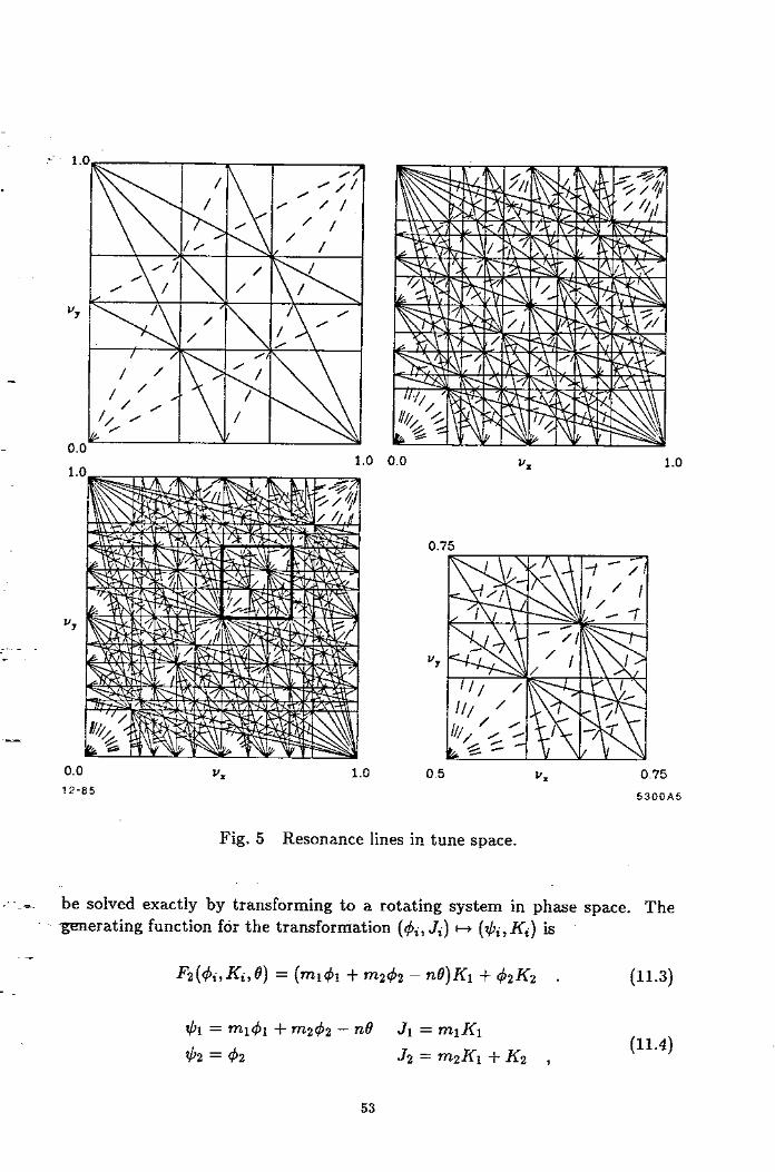
0.5 ux 0.75

5300A5

__

0.0 1.0 12-85

Fig. 5 Resonance lines in tune space.

_ . ._ :. be solved exactly by transforming to a rotating system in phase space. The - - -generating function fdr the transformation (q$, Ji) H ($i,K;) is

-

FdhKi,8) = (ml& + m242 - ne)Kl + 42K2 . (11.3)

-

$1 = m l& + w&2 - d 51 = rnlK1

$2 = 42 Jz=maKl+K2 , (11.4)

53

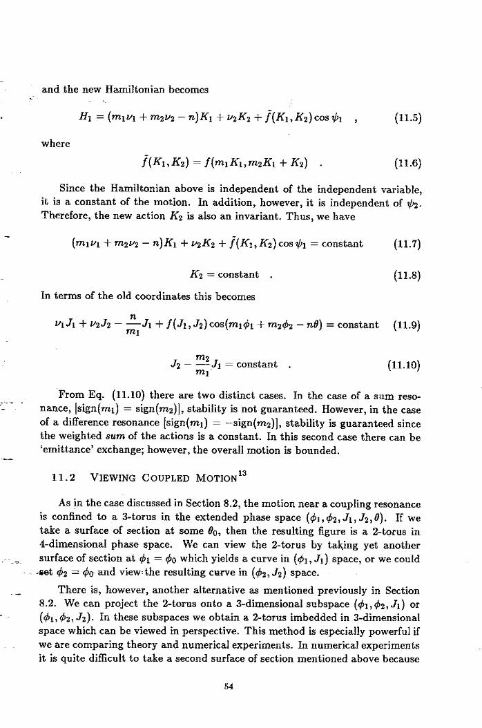
and the new Hamiltonian becomes L ,c-

. HI = (mm + mm - n)Kl + eK2 + f(Kl, K2) cos $1 , (11.5)

where

f”(KdG) = f(mdG,mdG +Kz) . (11.6)

Since the Hamiltonian above is independent of the independent variable, it is a constant of the motion. In addition, however, it is independent of $9. Therefore, the new action K2 is also an invariant. Thus, we have

(mryr + m2v2 - n)Kr + v2K2 + f”(Kl, K2) cos $1 = constant (11.7)

K2 = constant .

In terms of the old coordinates this becomes

(11.8)

VlJl +~2J2 - &JI +f(J1,J2)cos(ml& +m&. -rze) = constant (11.9)

- J2 - ~JI = constant . ml.

(11.10)

From Eq. (11.10) th ere are two distinct cases. In the case of a sum reso- ..-._ . - nance, [sign(mr) = sign(mz)], stability is not guaranteed. However, in the case of a difference resonance [sign(mr) = -sign(m stability is guaranteed since the weighted sum of the actions is a constant. In this second case there can be ‘emittance’ exchange; however, the overall motion is bounded.

11.2 VIEWING COUPLED MOTIONED

As in the case discussed in Section 8.2, the motion near a coupling resonance is confined to a S-torus in the extended phase space (~$1, $2, 51, J2,O). If we take a surface of section at some 80, then the resulting figure is a Z-torus in 4-dimensional phase space. We can view the Z-torus by taking yet another

_ . ._ - surface of section at 41 = ~$0 which yields a curve in ($1, 51) space, or we could - - -4 $2 = C#J~ and view: the resulting curve in (42, J2) space.

- There is, however, another alternative as mentioned previously in Section 8.2. We can project the Z-torus onto a 3-dimensional subspace (&,&, J1) or

- _ (41, 42, Jz). In these subspaces we obtain a Z-torus imbedded in S-dimensional space which can be viewed in perspective. This method is especially powerful if we are comparing theory and numerical experiments. In numerical experiments it is quite difficult to take a second surface of section mentioned above because

-

54

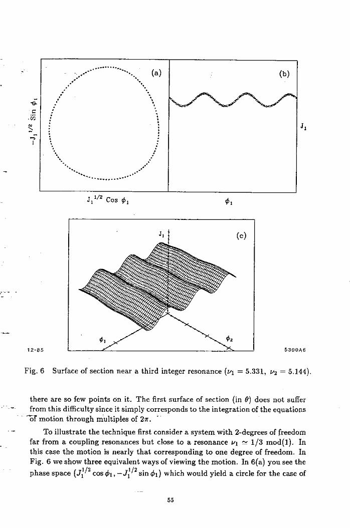
12-85

J11’2 cos $I -

5300A6

Fig. 6 Surface of section near a third integer resonance (VI = 5.331, ~2 = 5.144).

there are so few points on it. The first surface of section (in S) does not suffer _ ._ - from this difficulty since it simply corresponds to the integration of the equations - - -%f motion through multiples of 27r. :’

-

- _

To illustrate the technique first consider a system with Z-degrees of freedom far from a coupling resonances but close to a resonance ~1 N l/3 mod(l). In this case the motion is nearly that corresponding to one degree of freedom. In Fig. 6 we show three equivalent ways of viewing the motion. In 6(a) you see the phase space (J;/” cos t#q, -J:/” sin 41) which would yield a circle for the case of

--

55

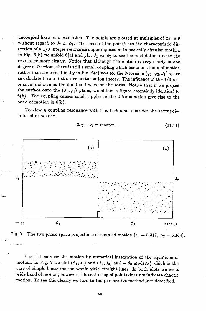
uncoupled harmonic oscillation. The points are plotted at multiples of 2~ in 0 ,CS- without regard to 52 or 42. The locus of the points has the characteristic dis-

. tortion of a l/3 integer resonance superimposed onto basically circular motion. In Fig. 6(b) we unfold 6(a) and plot J1 VS. 41 to see the modulation due to the resonance more clearly. Notice that although the motion is very nearly in one degree of freedom, there is still a small coupling which leads to a band of motion rather than a curve. Finally in Fig. 6(c) you see the 2-torus in (~$1, &,Jl) space as calculated from first order perturbation theory. The influence of the l/3 resonance is shown as the dominant wave on the torus. Notice that if we project the surface onto the (Jl, ~$1) pl ane, we obtain a figure essentially identical to 6(b). The coupling causes small ripples in the 2-torus which give rise to the band of motion in 6(b).

To view a coupling resonance with this technique consider the sextupole- induced resonance -

2v2 - vr = integer . (11.11)

w

. * .: -- ,. .* - *: -. . .: “a*

- .*. . . . - *. ._ . . .

: : :-* . :. :. . .’ . .

*. . . . . . - . . . . . -* * .* . . . . . * :

: . - . . . :a

. l

. . *-_.* ** . . . . .

, :-

. . * * ‘:. -* -..

* . : . 0 . :

. - . . . . . * . . .

. . . . . * .

. **-. . . : *

* . . . -* . . . * . **‘.

. .

* . . * .* . . .

. . . * :

. . : . .

- . * , * . * : * * - ). ** .

. :

- . . . * . . *.” * .* . . -_- . .

** ,

: : a.

-* . : * . . : . : . . * - : * -. ‘.’ . . 0. ,’ : :

-.. . : * . . , :* . . - .-. ; . . -*: . , . z .* . 1: .c: . . . * . . ; : : . . . . : :

J2

12-85 $1 $2 5300A7

Fig. 7 The two phase space projections of coupled motion (~1 = -5.317, ~2 = 5.164). 4 _ ._ :.

- L.

-

- _ First let us view the motion by numerical integration of the equations of

motion. In Fig. 7 we plot (~$1, J ) 1 and (42, J2) at 8 = Be mod(27r) which in the case of simple linear motion would yield straight lines. In both plots we see a wide band of motion; however, this scattering of points does not indicate chaotic motion. To see this clearly we turn to the perspective method just described.

56

-

_..._ . -

__ 12-85

Fig. 8 Surface of section near a coupling resonance (VI = 5.317, u2 = 5.164).

In Fig. 8 we show the surface of section 19 = 00 (mod 27r) near the coupling resonance. In 8(a) and 8(b) we plot the 2-torus as calculated with perturbation theory. Below in 8(c). and 8(d) _ we again plot all the data points obtained by

._ Tz numerical integration, The data fall nicely on the torus obtained by perturbation - theory. Notice that near a coupling resonance the surface is similar to that in

- Fig. 6; however, the ripples no longer run parallel to one of the axes.

- _ Using this technique it is possible in numerical experiments to separate chaotic motion from mere coupling. Chaotic motion is shown as departures from a surface similar to the departures from closed curves for the case of chaotic motion in one degree of freedom.

57

i ,c- 12. THE RESIDUE CRITERION 11’14

. In this section we begin the discussion of several techniques which address the question of the onset of chaotic behavior or the ‘breaking’ of KAM curves. The first technique, the residue criterion, developed by J. Greene applies only to cases of one degree of freedom (with a time dependent Hamiltonian). Since the renormalization discussed in Section 14 was founded on the residue criterion, it too is limited to systems in one degree of freedom.

.Greene’s approach to the onset of chaotic behavior focuses on one particular invariant curve with some irrational tune or winding number w to determine the perturbation strength which causes the KAM curve to ‘break’. The basic idea is that the distinction between w and very good rational approximations to w, wn = pn/qn, should not be very great. Here p, and qn are two relatively prime integers. But in fact we know that the orbit for a rational frequency consists of a sequence of 2q, points in phase space which are periodic orbits, while an invariant KAM curve with irrational tune gets filled in densely as time progresses. In spite of this difference perhaps the existence of a KAM curve is related to properties of the neighboring periodic orbits.

- 12.1 THE DEFINITION OF THE RESIDUE

A key property of a periodic orbit is its stability. We know how to calculate _..._ . - stability of an arbitrary periodic orbit from the analysis in Sections 3.3 and 5.1.

The procedure is:

1. First locate a periodic orbit (closed orbit) with some period %q,.

__ 2. Linearize the equations of motion about the fixed point (or linearize the map of initial conditions to final conditions about the fixed point.)

3. Calculate the transfer matrix A4 for one period (2rqn).

4. Calculate the trace of M (a 2 x 2 matrix).

5. If /Trace(M)1 < 2, then the fixed point is stable.

So the procedure is identical to the analysis of betatron oscillations. Why _ . ._ -. should one use the properties of a periodic orbit rather than those of the island

- _ -grounding it (for example the width) ? The stability properties of periodic orbits can be determined exactly without ambiguity while the concept of width

- breaks down just when the widths of islands get large. - _ Unfortunately, it is not just stability which determines the existence of KAM

curves since there are equal numbers of stable and unstable periodic orbits neighboring a KAM curve. However, the trace of the transfer matrix is still a good candidate for a key parameter. Rather than the trace Greene uses the

-

58

residue R defined by i ,c-

. R = $2 - Trace( ,’ (12.1)

where i& is the matrix for the one-period map near the periodic orbit with period 2rq. If we define a ‘tune’ e in analogy to the tune in betatron oscillations, then

cos 2rt = TraceM

2 ’ (12.2)

and

R = sin2 ~6 . (12.3)

To get the idea let us first state the qualitative version of Greene’s empirical residue criterion:

1. Check the residue for periodic orbits ‘close’ to the KAM curve in question. 2. If /RI < l/4, the neighboring KAM curve probably exists. 3. If IR > ]1/4, the neighboring KAM curve probably does not exist.

The question is which periodic orbits do we check and how do we improve the accuracy of the method in a systematic way. This leads us to a brief discussion of continued fractions.

- 12.2 CONTINUED FRACTIONS

_._._ . - Every irrational number w has a unique continued fraction expansion. This

leads to a sequence of rational approximations w, = p,/q, to w which are the ‘best’ for a given size denominator. That is, all other rational approximations to w with denominators less than or equal to qn are further from w than the con-

__ tinued fraction approximation p,/q,. If we write p,/q, for the nth approximate, then

Pn 1 -=uo+ Qn a1 + @+ l 1

(12.4)

‘*. +&

which is more conveniently written

Pn - = _ Qn [ ao,al,---, an] - ._ Tz - - --

The frequency w can‘then be written’ -

- _ w= lim p,.

n--rm Qn

(12.5)

(12.6)

-

To each of these elements pn/qn there corresponds a periodic orbit in phase space. These periodic orbits and the resonance islands surrounding them tightly squeeze the KAM curve with tune w.

59

12.3 A PRECISE STATEMENT OF THE RESIDUE CRITERION c ,c-

. We are now in a position to state the residue criterion precisely. Consider a KAM curve with tune or winding number w. Consider the sequence of approxi- mates pn/qn in the continued fraction representation of w. Examine each of the residues R, of the periodic orbits with frequency pn/qn. Then there are three distinct cases:

1. Rn + 0, n + 00; there is a KAM curve with winding number w.

2. Rn + foe, n -+ 00; there is no KAM curve with winding number w.

3. Rn + &, n + co; the transition case.

Best convergence is achieved for Ro around l/4, but that depends upon w. It is important to note that the criterion above can in principle yield very precise results on the breaking of KAM curves. For example Shenker and Kadanoff in Ref. 15 have determined numerically that the critical residue for breaking a KAM curve with a winding number equal to the ‘golden mean’,

7= 1+&

2 (12.7)

- is given by

R, = .2500888 . (12.8) _..._ . -

In addition this criterion suggests that there is an asymptotic serf simihjty at the critical case since all the residues are equal. We return to this question in Section 14.

12.4 AN ISOLATED RESONANCE EXAMPLE

To calculate an example let us return to the isolated resonance Hamiltonian of Section 10.4. From Eq. (10.18) the H amiltonian in the neighborhood of the resonance v N n/m is given approximately by

_ ._ - - HT 3 y (J - JJ2 + f(Jr) cos rn& + - -- . (12.9)

-

- Recall that this Hamiltonian is expressed in coordinates which rotate in phase space (see Eq. (10.3) to (10.5)). In th ese coordinates there is are 2m fixed points at J = Jr and 41 = Icalm, k = 1,2, --. 2m. In the original coordinates these are periodic orbits with period 2rm. Following Section 10.3 we linearize about one of these periodic orbits and find that the frequency of oscillation in

60

the $1 coordinates is ,--

Now we must construct This is simply given by

(w\ ( cos ne sin ne/a”(J,> \ ( h(O) \ \bJ(d)) = \o?(Jr)sinR6 cosn6 ) \6J(O)) ’

R2 = cx”(J,.)f(Jr)m2 : (12.10)

the matrix transforming motion about the fixed point.

If we construct the matrix for one period (2rm) and recognize that 4 and 41 simply differ by 27r in this case, we find the one period matrix to be

iv, = cos(27rmfl) sin(2zmn)/a”( Jr)

a”( Jr) sin(2rmn) > cos(27rmR) ’ (12.12)

Calculating the trace of the matrix above and using Eq. (12.1) yields the residue for this example,

R = sin2(zmR) . (12.13)

- This approximate approach can be used to check the existence of neighboring KAM curves to known resonances. In the more precise approach one must locate the periodic orbits numerically, and calculate the matrix Mq numerically.

- .- . This must be done for higher and higher order resonances. Because of this, much - of the work with the residue criterion has been devoted to the study of nonlinear

mappings. These avoid the problems associated with tedious numerical integration of differential equations to locate fixed points and calculate residues. In the mapping case the differential equations have effectively already been integrated through 27r in 8 the independent variable. Integration in 8 is thus replaced by simple iteration of the map.

13. DIRECT SOLUTION OF THE HAMILTON-JACOBI EQUATION 16’17

_ ._ Tz In the previous sections we have seen the utility as well as some of the limi- _ _&&ions of perturbation theory. For small perturbations and- far from resonance

perturbation theory gives an accurate description of the small distortions of the -

- _

invariant surfaces; however, it completely misses the small neighboring islands and regions of chaotic behavior. This is due to the non-convergence of perturbation theory in most cases. There are very special circumstances described in the KAM theorem which permit one to calculate invariant tori which, however, are not continuous families (as one expects in integrable systems). This is true

61

because the tune of the actual motion along the KAM curve in question must .+-

. be irrational-or in two or more degrees of freedom, the frequencies of motion on the KAM torus must be incommensurate. However, since the rational numbers are a dense set, just next to any irrational is a rational. Therefore, between these invariant tori lie regions of resonance islands and chaotic behavior.

In this section we move beyond perturbation theory to develop a method to calculate directly KAM tori and estimate the strength of the perturbation necessary to break a given invariant curve. The aim is to achieve better results in the neighborhood of resonance, and also to achieve good results in the neighborhood of chaotic motion. We follow Refs. 16 and 17 throughout this section.

13.1 THE HAMILTON- JACOBI EQUATION

In this section we begin as in Section 7 but restrict the problem to a system with one degree of freedom for simplicity. In a circular accelerator this corresponds to motion in one transverse degree of freedom. The Hamiltonian we consider is given by

H(46, J,e> = HO(J) + V(A J,e), (13.1)

- where 8 is the machine azimuth or ‘time’, and the perturbation V is periodic in 8 and C$ with period 27r. To obtain the Hamilton-Jacobi equation, we seek a canonical transformation (4, J) I+ ($, K) in the form

_..._ _ - J=K+‘+&W,~), (13.2)

ti = ++G&#a,q , (13.3)

such that the new Hamiltonian becomes a function of K alone. Once again subscripts denote partial derivatives. The Hamilton-Jacobi equation to determine the generator G is the requirement that the new Hamiltonian HI indeed depend only on K; namely

_ . -2.

Ho(K + G4) + V(4,K + G4,8) + Ge = HI(K) . (13.4)

If we succeed in finding .G, then by Hamilton’s equations in the new variables, K will be invariant, and + will advance linearly with the time:

.- K = constant ,

ti=h(W+lCIo ,

where aH1

VI(K) = dK (13.6)

(13.5)

-

is the perturbed frequency.

62

.

c As in Section 7 we are interested in solutions of (13.4) which are periodic .+- in both 4 and 8 since we are interested in the distortion of the invariant torus.

. This leads us to use the Fourier development

G(c#+ K, 0) = c gmn(K)ei(m4-ns) . m,n

(13.7)

It is useful to rearrange (13.4) by adding and subtracting terms so as to isolate terms linear in G# and Go. We then take the Fourier transform for m # 0 to cast.Eq. (13.4) in the form

g = A(s) , (13.8)

where g = [gmn] is a vector of Fourier coefficients and

2r 2n

Amn(g) = (v(K): - n) (2i)2 JJ d~&je-i(mb-ns) x

0 0

-

(13.9)

[H(hK + Gg,e) - Ho(K) - v(K)G4] , m # 0 ,

-

where v(K) = cYHo/dK. N o ice that if we set G# to zero on the right hand side t’ of Eq. (13.8), we obtain the Fourier coefficient for the generating function of first order perturbation theory as in Eq. (7.15). Equation (13.8) is a nonlinear algebraic equation for the Fourier coefficients gmn which is equivalent to the

_.__ _ nonlinear partial differential equation for G. -

To truncate the system of equations (13.8) and (13.9) for numerical solution we restrict (m, n) to some bounded set B of integers, with m # 0, and put

__ G4= c imgmn( K) ei(m’#‘-nO) . (13.10) (m,n)EB

In an iterative solution of (13.8) the set B is selected so that at iterate (p + 1) all Amn-(g(P)) with (m, n) E B are greater than some preassigned small number; here g(P) is the pth iterate.

It is important to note that only the amplitudes gmn for m # 0 are required _ . _ _Y_ to calculate G$; the m = 0 amplitude and also the function HI(K) can be

-.._ determined from (13.4) a posteriori. Qnce G# is known, the-distorted invariant curve may be obtained from Eq. (13.2) by taking a surface of section at some

- 80 and plotting J(& 00) US. 4. The new action K is constant by Hamilton’s - _ equation and is thus an input parameter.

The equation in the form (13.8) is suitable for the examples treated below, but not for typical accelerator problems involving short nonlinear lattice elements. For the latter, the Fourier analysis in 8 has slow convergence and should

63

be avoided. For an accelerator lattice we retain the Fourier analysis in 4, and use i .+- the periodic Green function for the operator imv+3{dtJ, as shown in Eq. (7.12).

. This leads to an integral equation for the amplitudes gm(K; 0) which can be dis- cretized to provide an equation for the variables gm.(K; d,), m 2 1, where the 8i are mesh points located only in the nonlinear elements of the lattice. The solu- .tion is periodic in 8 because we use the periodic Green function. An alternative procedure is to treat the equation as a system of differential equations in 8. The equation must be integrated only once around the accelerator with periodicity achieved by iteration, in analogy to nonlinear closed orbit calculations.

13.2 AN INTEGRABLE EXAMPLE

Before trying the method on nonintegrable cases it is useful first to test the method on an integrable example. In this section we show results from

- solving (13.8) - (13.10) by Newton’s method (starting from g = 0). This first example is a locally integrable case in which some of the invariant surfaces may be expressed analytically, namely the 4th order isolated resonance model with

-

H@, J, 0) = VgJ + aJ2/2 + cJ2 cos(4qi - 6’) , (13.11)

where ~0, Q, and E are constants. .This example has been treated in detail in Ref. 16; here we present some of the more difficult cases which were calculated.

6-66 d/J coscp 5511A6 Li co+ 5511A3

-

Fig. 9 4th order resonance, (a) H-J solution (b) Exact solution

64

The most difficult curves to compute are the separutrices around wide is- .+- lands. In this-case first order perturbation theory gives very poor results. How-

. ever, the direct solution of the Hamilton-Jacobi equation works surprisingly well in this case as is seen in Figures 9(a) and 9(b) Fig. 9(a) shows separatrices computed in 9 iterations with 31 modes in the set B. The points are plotted in normalized phase space (0 cos C$ us. fisin 4) at 8 = 0. The inner separatrix (almost a square) and the outer separatrix (four lobes intersecting at right angles) are from two different calculations for two different values of K. Fig. 9(b) is a plot of curves from the exact analytic formulas for comparison. The.separatrix curves and curves both outside and inside the resonance islands are included to guide the eye. The Hamilton-Jacobi solution is virtually indis- tinguishable from the analytic curves. This test case is not simply academic since accelerators typically have small nonlinearity which yields large islands (or unbounded motion). In regions close to single resonances in nonintegrable systems similar results are obtained although the separatrix in this case cannot be calculated since it is a thin band of chaotic motion. This leads us to the next section where we show a nonintegrable example.

13.3 THE Two RESONANCE MODEL

- This second example is nonintegrable and contains all the generic phenomena of nonlinear mechanics in 1; or’ 2 degrees of freedom. In restricted regions of phase space it should describe the essential features of one dimensional beta-

_...._ _ - tron motion in the presence of nonlinearities. The example is the two-resonance model with the Hamiltonian

H = voJ + ;aJ2 + q J5f2 cos(54 - 38) + c2 J2 cos(8qt - 58) . (13.12) .-

Equations (13.8) - (13.10) are solved with Newton’s method for the invariant curve with a tune equal to the golden mean u* = (& - 1)/2, which is between the two resonances. Here Y, is the exact perturbed tune, Y, = dHl/dK, not the unperturbed tune u = ue + aK. To maintain the perturbed tune at the preassigned value, we include the equation u* = dHl/dK as a constraint in the iteration (see Ref. 16). -This process is repeated for a sequence of resonance

_ , _T_ strengths ~1, ~2 (arbitrarily taking ~1 = 2~2) beginning with moderate strengths ---- -tu-look for the transition to chaotic behavior.

- The other parameters are chosen to be uc = 0.5, cx = 0.1, which places the resonance islands of the two resonances near J = 1.0 and J = 1.25. The sequence of resonance strengths and resonance half-widths A Jl, A J2 shown here are as follows:

-

C

(i) cl = 2c2 = 6 x 10-5, A Jl = 0.049, AJ2 = 0.054. 3

65

._ (ii). ~1 = 2~2 = 10-4, AJl = 0.063, AJ2 = 0.070; '- (iii) Cl z--g = 1 .25 x 10-4, A Jl = 0.070, AJ2 = 6.078;

By the Chirikov resonance overlap criterion,l’ the corresponding invariant curves should be close to breakup, since the resonance separation is Jr1 - Jr2 = 0.25.

13.3.1 A New Criterion for the Break-up of a KAM curve

In Ref. 16 a new criterion is proposed for the break-up of a KAM curve, the ‘transition to chaos’. The criterion is that the Jacobian of Eq. (13.3) vanish at some (4,0) as the E’S are increased:

%!‘/W = 1 + GK~ = dJ/dK = 0 . (13.13) -

At such a point it is in general impossible to solve uniquely for 4 as a function of $. To qualitatively understand the idea first write the solution for II, assuming the Hamilton-Jacobi equation has been successfully solved. This is given by

- Therefore we have

ti=+o+u*e. (13.14) . . .

_..._ . -

ati WO -- q- aqc

(13.15) - :

The heuristic picture is then that if we infinitesimally change the initial condition for motion on the invariant curve, the phase motion (4) on the curve mapped into the original coordinates jumps discontinuously. This would not happen on .v a smooth continuous invariant curve, but might happen on a curve with gaps.

Before continuing the discussion of results of the two resonance model it is interesting to conjecture the generalization of Eq. (13.13). The key point is the non-invertibility of (13.3). In higher dimensions the conjectured criterion is that the determinant of the Jacobian matrix of the second canonical transformation equation vanish. If we denote the old and new vector angle variables with bold face, then the second canonical transformation equation becomes C

_ , _T_ ~- -- iz*- L

*==++GK(*,K,~), (13.16) -

while the condition for the break-up of the KAM torus is

Det(a$F/a@) = Det(I + GQK) = 0 . (13.17)

66

1 , / , , , , , i

2.0 - (b)

1.6 -

a+ ‘*’ G

:;:

I 1 I I I I 1

0 0.2 0.4 0.6 0.8 1.0 0 0.2 0.4 0.6 0.8 1.0

(I-86 +/2r 5511110 +/2= 5511114

Fig. 10 (a)Th e invariant curve and (b) a$/&$ for 61 = 2~2 = 6 x IO-~.

- 13.3.2 Invariant curves and their break-up

Figures 10(a), 11(a), and 12(a) show the invariant curves for the two res- _..._ . onance model in Cartesian plots of J(qS,O = 0) for cases (i), (ii) and (iii) - respectively. Figures 10(b), 11(b), and 12(b) give the corresponding plots of

&j/&$(4,8 = 0). The latter quantity allows us to test condition (13.13), since the minimum values of a$,/@ are quite insensitive to 8. The anticipated zeros

_u of a$/@~ are on the verge of appearance in Fig. 12(b).

In Figures 13(a), 13(b), and 14(b) we show enlargements of small portions of the invariant curves for cases (i), (ii) and (iii), together with points obtained by tracking from initial conditions on the appropriate curve. An orbit from a single initial condition was followed through N turns in 8, with N = 4000, 4000, and 1500 for cases (i), (ii) and (iii) respectively. The good agreement between tracking and computed curves indicated in Figures 13(a) and 13(b) is maintained

_ . ._ - over the full range of 4. Chaotic behavior is evident in case (iii), but completely __ &sent in case (ii). In Fig. 14(a) we show an intermediate case, ~1 = 262 =

1.2 x 10m4 tracked for 3000 turns, which is ambiguous. It might represent a - broken KAM curve or merely a high-order island chain not yet filled in. The

scatter of points in Figures 14(a) and 14(b) ’ g IS enuine, since the accuracy of the integration of Hamilton’s equations has been checked by integrating back to the initial conditions.

Comparing Figures 12(b) and 14(b) one sees that condition (13.13) is first

-

67

.

0 0.2 0.4 0.6 0.8 1.0 0 0.2 0.4 0.6 0.8 1.0

8-86 +!2r 5511A12 (P/27 5511A16

-

Fig. 11 (a)Th e invariant curve and (b) &j/&j for ~1 = 2~2 = 1 x 10e4.

_..._ . 1.20 -

I. 18 ._ J

1.16

I. I4

I .6

dJ I .2

JR 0.8

0.4

0 0 0.2 0.4 0.6 0.8 1.0 0 0.2 0.4 0.6 0.8 _ 1.0

_ ._ - - 8-06 #J/277. 5511*13 e-w 4#/2r 6111A18 -.._ ia*- L.

.- Fig. 12 (a)Th e invariant curve and (b) &j/a4 for ~1 = 2~ = 1.25 x 10m4.

met at roughly that perturbation strength at which chaotic motion appears in tracking. Actually, the Hamilton-Jacobi results for &+!~/a4 (but not those for J) are slightly ambiguous for ~1 = 2~2 > 10A4, since at such large perturbations

68

.

-

_..._ -

__

,--

J

I.1884 I.195

I.194 I. I883

I.193

I.1882 I.192

I. I 880 I.190 0.248 0.250 0.252 0.24 0.25 0.26

6-66 +/2r 5511A19 $427 55llA20

Fig. 13 Invariant curve us. numerical solution, (a) case (i) and (b) case (ii)

1.205

I.195 J

I.190

I . I 85

(a) ; 11

(b) 1

I.180 -0.20 0.24 0.28 0.20 0.24 0.28

6-66 +/2r 5511A21 w2* 5511A22

Fig. 14 _ Invariant curve us. numerical solution, (a) ~1 = 10S4 and (b) case (iii) _ ^T_

- L.

-

-

- _

there is a limitation on the number of modes that can be accommodated while retaining convergence of Newton’s method. Thus one cannot say precisely where (13.13) is first satisfied. A more precise determination of the transition should be possible by using a second canonical transformation or a modification of Newton’s method. Assessing the results from tracking and &j/$4 together, the

69

curve for the golden mean tune breaks up at ~1 = 2~2 = (1.2 f .05) x 10w4. ,--

The Hamilton-Jacobi method provides a promising alternative to canonical perturbation theory and its modern variants. Unlike perturbation theory its algebraic complexity does not increase as more accuracy is demanded, and the required computer programs are quite simple. The criterion in Eq. (13.16) for the transition to chaotic behavior in higher dimensional systems may provide a useful criterion for the break-up of KAM tori in the full 5-dimensional extended phase space of betatron motion. The reader interested in more details of this method should consult Ref. 16.

13.4 A COMPARISON WITH THE RESIDUE CRITERION

In this section we would like to make the connection between John Greene’s residue criterion 11,14 and the associated Hamilton-Jacobi equation. To do this we need to solve the H-J equation over a finite time interval, locate an appropriate fixed point of the resulting map, and linearize about that point to calculate the residue.

-

To solve the H-J equation over a finite time interval it is necessary to re- specify the problem and convenient to change notation slightly. We consider a canonical transformation (4, J) I+ (di, Ji) defined by

- .- . J = Ji + S&k JiA4) , - ~TI = 4 + $Ji(d’, Ji,‘,‘i) 3

(13.18)

.- where f$ is the initial time. The H-J equation which is appropriate for the finite- time map consists of the requirement that the new Hamiltonian be identically zero

H(4, Ji + i&,6) + $8 = o . (13.19)

In this case the new coordinates are the initial conditions provided that we also impose the boundary condition

_ _ _T_ S(d, Ji&A) = 0 - (13.20)

In this case G is not a periodic function of 6; however, it does satisfy

$(A JdJ + 2~4 + 274 = S(d, Ji,Wi) ,

-

-

since the original Hamiltonian is periodic in 8.

70

To study the neighborhood of a periodic orbit with period 2rq, we note that ,L. such a periodic orbit is a fixed point of the map in .(13.18) at (~$0, Jo) provided

. that S&o, Jo,4 + 2w&) = 0 ,

$Ji(dO, JO,‘i + 2rq,‘i) = 0 (13.21)

*

To calculate the residue of that fixed point we linearize for small deviations about it by setting

4 = do + 64 , 4i = 40 + M , J= Jo+bJ, Ji= Jo+6Ji.

(13.22)

From (13.18) ‘f 1 we now keep terms linear in the deviation from the fixed point we obtain the linear map

(:i) = l:$$J (

0 + Ad2 - &&JJ $44 -$JJ 1 ) (662) ' (13'23)

-

where all partial derivatives of $ are evaluated at (40, Jo, 19; + 2rq, Si). Denoting the- matrix above as M,, the frequency or tune V~ of the oscillation about the fixed point is given by

- .- -

Trace(Mq) = 2 cos 27~~ = l+ (1 + $4~)~ - S&JJ 1 + &J

. (13.24)

Therefore, the residue is given by”

.-

R = a[2 - Trace( = f ‘~~f~~~f~J2 >

. (13.25)

In the case of an integrable system with Hamiltonian Ho(J) we find

9 = -Ho(J)0 (13.26) _ _ ._-. which yields R = 0. : L.

In the case of a nonintegrable system we test the existence of some KAM - curve with irrational frequency w by considering the residues R, of a sequence of periodic orbits of increasing period 2rq, as n + 00. The elements of the sequence correspond to frequencies in the continued fraction representation of f-4 say pl/ql, P2lq2, -- According to Greene there are three distinct cases:

1. R + 0, there is a KAM curve with frequency w.

-

C

71

2.- R + foe, there is no KAM curve with frequency w. ,c-

3. R * &, the transition case. .

If attention is restricted to solutions 5 with bounded second derivatives, then case (2) can arise only if

1 + $,jJcn) + 0, n + m . (13.27)

This recalls the condition that 1 + G#K should first acquire a zero at transition; cf. Section 13.3.1. The latter condition refers to the G which generates an orbit covering an invariant surface, which is a different object from the $cn) of (13.27). Nevertheless, for large n the orbit generated by S(n) lies close to the surface generated by G. The failure of either condition, 1 + $#Jcn) # 0 or 1 + G#K # 0, means that the corresponding canonical transformation, (13.18) or (l3.3), is no longer well defined. It seems reasonable that the two conditions (the former taken in the limit n + 00) should fail simultaneously as parameters approach critical values.

14. RENORMALIZATION: THE ROUTE TO CHAOS

- .In Sections 10.3, 10.4, 12 and 13.3.1 we discussed techniques for determining

the existence of invariant curves in non-integrable systems. In this section we continue by discussing the renormalization explanation of the break-up of a KAM curve.

_._._ . - The residue criterion discussed in Section 12 is the driving force behind renormalization. Consider a KAM curve with a golden mean tune or winding number. Then examine the sequence of resonances which squeeze this KAM curve as discussed in Section 12.2. Then there is a critical case in which the

.-L-s residues of the periodic orbits with longer and longer periods are all equal. This leads one to suspect an asymptotic self-similarity between these resonances which suggests that a renormalization approach might be useful.

The basic idea is then to find some transformation which links the properties of large islands about periodic orbits with low periods, to the properties of smaller islands about periodic orbits with longer periods. Once this transformation is obtained, one can-calculate the critical residue and study the properties

_ . ._ - of this self-similarity.

- To illustrate this technique we consider the two resonance problem. First we - covert it to a convenient form, then we calculate the renormalization transfor-

mation approximately, and finally we study the renormalization group obtained. - _ The technique used here is similar in spirit to Escande and Doveil in Refs. 18

and 19, but the results obtained are equivalent to those obtained by Greene and MacKay in Ref. 20. For complete discussions of renormalization & Zu MacKay and Greene see Refs. 14, 21, and 22.

-

. .

72

14.1 THE Two RESONANCE MODEL i ,c-

. In this section we consider a slightly different form of the two resonance model to begin renormalization. This form is inspired by the two resonance model of Escande and Doveil. 18,19

We begin with the Hamiltonian

H = UOJ + crJ2/2 - EI COS(~& - n16) - ~2 COS(UA~~~) - n26) , (14.1)

where ~1 and ~2 in this case are constant. We would like to convert this problem by changes of variables to one very similar to that considered by Escande and Doveil, namely

u = ;-Ccosg-Dcos(k~-t). (14.2)

This can be accomplished with a sequence of transformations; however, before beginning it is useful to introduce two types of scaling transformations which will be used together with the more standard canonical transformations.

-

14.1.1 Scaling The Time and the Momentum

- -To begin it is useful to write down Hamilton’s equations since the scaling

equations can then be read off by inspection. In the old variables Hamilton’s equations for the coordinates and momentum (q,p) are

. .

_._._ . - dq dH dp dH -- z-dp ’ z=-aq *

(14.3)

First we would like to change the scale of the time variable while preserving the form of Hamilton’s Equations. If we change to a new variable t’ given by

__ t’ = at , (14.4)

then the form of Hamilton’s equations is preserved if we set

H’ = H a -

(14.5)

It is also useful at times to scale the momentum. While this does not preserve the Poisson bracket, it simply multiplies it by a constant. In this case _ ._ -. a simple scaling of the Hamiltonian once again preserves the-form of Hamilton’s -.._ - equations. Inspecting Hamilton’s equations in Eq. (14.3) we see that if

- P’ = XP 3 (14.6)

- _ the form of Hamilton’s equations is preserved provided that

H’=XH. (14.7)

73

14.1.2 The ‘Standard’ Form of the Two Resonance Problem L ,c-

. Now to convert the starting Hamiltonian of Eq. (14.1) to the standard form we begin with the canonical transformation ($, J) H (4, Jr)

cj = rnr$ - nr0 J=mlJl (14.8)

HI = H-nlJl ,

which yields the new Hamiltonian

m9 2 HI = (mluo - n) 51 + c”2J’ - ~1 cos 4 - e2 COS(~~ - $8) (14.9)

- where k=m%

ml (14.10) A = n2ml - nlm2 .

Next we would like to scale the time variable. Following the previous section this can be done by setting

t=Ae ml

which yields the new Hamiltonian

__ 4 2 ff2 = ~[(mivg - nl)J1 + 2 Jl]

- Tel cos 4 - Tc2 cos(k$ - t) .

(14.11)

(14.12)

Before scaling the momentum it is useful to complete the square in the &independent part of~H2 to yield _ ._ - - H2 = “;’ -(Jl - jl”)” - 7 co;4 - 7 cos(kcj - t) < const , (14.13)

.-

where - _ J1” = nl - mu0

am!

-

Finally we shift the origin and scale the momentum variable with the transfor-

74

mation ,-- . . .

. P= 2(Jl _ J,“)

which yields the final desired form

where

_._._ -

U = ;-Ccosc+GDcos(kqLt) ,

C2$ A2

D=am:,z. A2

(14.14)

(14.15) -

To summarize the sequence of transformations, we collect the changes of variables and the associated parameters below,

k=?.? A = n2ml - nlrnz , ml ’

4 = ml+ - we t=%, ,. ml (14.16)

%(Jl -J,“) , J1” = nl - n-w0 P= am! ’

In these new variables the resonant amplitudes for the two resonances have been shifted to

PO = 0 pl N l/k .

(14.17)

Using the analysis of Section 12.4 the residues at the stable periodic orbits are given approximately by

& II ?r2c

R1 N ?r2k4D . (14.18)

75

“

. Strength Resonant tune Strength Resonant tune

El El EL EL ml ml

62 62 EL EL m2 m2

6 6 2E.L 2E.L 2ml 2ml

4 4 2% 2% 2m2 2m2

El E2 El E2 n1+n2 n1+n2 ml+m2 ml+m2

Cl E2 Cl E2 n1-n2 n1-n2

ml-m2 ml-m2

. . . . . .

14.2 THE RENORMALIZATION TRANSFORMATION

In keeping with the residue criterion we would like to examine the sequence of higher order islands which comes from the continued fraction representation of the frequency we are considering. If we express the sequence of resonances given by the rule

- n3 nl + n2 -= m3 ml-l-m2 ’ n4 n2 + n3 --.- . -=

- m m2+m3, (14.19)

we find that this sequence lim its on the irrational tune -

r= nl + 7n2

ml+-im2 ' (14.20)

where

+Y= 1+&

2 - (14.21)

These numbers are called Noble numbers and the sequence generated is the con- _. ’ ._r. t inued fraction representation of the Noble number I’. The approach described

- - -here focuses on just these types of irrational numbers.

- The two resonance terms which appear explicitly in the Hamiltonian gener- ate two sequences of driving resonance islands about their stable periodic orbits

- _ as discussed in Section 10. In addition, their interaction generates an infinite number of other fixed points and resonance islands. To see this explicitly in perturbation theory we can use the analysis in Section 7 to show that the resonances follow the sequence shown in Table 1.

-

-

76

i ;‘

.

-

- - . . . - .

L

- -

P

0 ,t . .- . . ..- 0.8

‘.

‘1. ..... ,.. . ..’ . .

. . . . . .

I I I I I I I I I I I I I I f I 1 I

I I I I I I 1 I I 1 I I , I I I I 8 I I

(b) -

0.7

,d. . -. I’ *

i- ‘Y s \ . . .

I ’ --. ..’

P

0.6

0.5

. ‘. -. - a>: ., ‘b., : c -,... J&&f’ . . . . . - . ..I . . . .-. I’ f ‘,,. - .,v.y.. . . - ,Q.>.. -7. ‘.-*sG ,... - c . . ’ ...:.:.“.L \ .., ;\ . .-= ,.:.:‘,+ . . ‘X. . , ” 6. ‘8

l ;~~;;:2-~~~~~~,~-~~~-~~~.. I . , . ; - --?.A ~... . . . . . . ..- &z:.::.*- - - L”- *

- - : .

--a-.. ::i ‘.., .’

.r . . . . .

, . . I . . . . . . . , .* . , ? * .

. , +.’

‘, P

.‘.:.,

/

.:’ ,

. . :

.@$+

.;

i: .:;’

‘.;l,,. $$

j.” “i

k:,.-” $

. -: 8”’ :

a-’

. .

k .

. .

*a-’ “\,

. . . . . . . . -. . .

. . . .

I 0 I I I I I I I

,..:.v.“-‘t :.. ‘i, I ’ ’ ’ ’ . . . .

..a .i ...< .*.‘.. “.I .,. (a) _

,r,C” .:. ;: _

I’ ‘x.

o.4 ;y., , , 1 , , , I 1 , , , ( 1 , , , , 1 8 t-1

0 0.2 0.4 0.6 0.8 1.0

12-86 ;’ +/27r 5618A16

Fig. 15 The Two Resonance Model (k = 1).

77

To see this in a specific example consider the standard two resonance Hamil- i .%‘ tonian in%q: (14.2) with k = 1. In Figs. 15(a) and 15(b) you see plots of the

. motion in phase space (a surface of section at t = 0 mod 27r) generated by integrating Hamilton’s equations for this case. In .Fig. 15(a) you see the two driving resonances centered at 4 = z and p N 0, 1.0. Each sequence of islands is of course generated by a different initial condition integrated through many multiples of 2~. Between the two driving resonances you see a sequence of resonances. In Fig. 15(b) th e momentum scale is blown up to show the detail of the higher order resonances. The ‘dashed’ curve in the center of Fig. 15(b) is a KAM curve with a tune or winding number of l/7. The sequence of resonances shown are just those which correspond to the continued fraction approximations to l/r, namely O/l, l/l, l/2, 2/3, 3/5, and 5/8. Note that the resonance islands rapidly squeeze the KAM curve and impress their shape on it causing it to weave through the gaps between the resonance islands. The sequence of resonances shown are those which must be checked with the residue criterion to see if the KAM curve exists. Notice that the island widths are rather ill defined due to some chaotic behavior and also due to the distortions of neighboring resonance islands. It is just this sequence of resonances which we focus on in this section. The elements of this sequence are obtained by simply adding both the numerators and denominators of the previous two resonances. Therefore, in

- the remainder of this section we will focus on resonance phases which add since these limit on the noble number which is between the two driving resonances.

The basic idea is to find a transformation of the Hamiltonian which allows --...- . L us to study the next higher order periodic orbits in this sequence and their associated resonance islands.

To begin this process we perform a general canonical transformation close to the identity similar to that used in perturbation theory in Section 7. Consider the canonical transformation (p, 4) H (PI,&) generated by

fih4~1J) = 4~1 + G@,pl,t)

with the transformation equations

_ . -1.

-.-

Then the new Hamiltonian is

61 = 4 + G,, P=P~+$

HI ?,U +Gt ,

G2 - _ ul =~+~+PIGm+Gt-Ccos~-Dcos(k~-t)

(14.22)

(14.23)

(14.24)

-

The simplest choice for the generating function is the choice which eliminates one of the explicit resonances from view, but yields explicit higher order resonances

78

i in the new variables. Therefore we set ,;”

. plG4 + Gt = CCOS~ (14.25)

which yields

G = isin (14.26)

If we now complete the substitution of new variables, and keep up to quadratic terms in the strength of the resonance we find

2 c2 Xl = 2+&l+

CD cos2$~1)-Dcos(krj5~-t)+- sin(bh -t) sind+. . . . (14.27)

1 p!

We wish to study the interactions of two resonances in which the phases add, since these resonances are closer and closer to the Noble frequency I which lies between our initial two resonances. The other resonances are far away in phase space and will simply be dropped here. This yields

- h = $ - Dcos(k& - t) - FCOS[(I + k)& - t] + . . . ,

1 (14.28)

L

.-

which is once again a two resonance Hamiltonian but with one of the driving resonances and the next higher order resonance. To obtain the exact form of the two resonance Hamiltonian which we started with, we must approximate the coefficient of the new resonance. To preserve the residue and for small island width we can set pl to its value at the center of the island

1 Pl = l+lc

which yields

(14.29)

_ . ---w I1 = $ - Dcos(kh - t) - Ic(’ +:zk)zcD cos[(l + k)& _ t] + . . . . (14.30)

-

-

- _ Now that we have the new Hamiltonian in the desired two resonance form,

the next step is to make a sequence of transformations to convert this Hamil- tonian to the one which we started with. This, however, is quite easy since we have already taken a more general Hamiltonian of this form in Eq. (14.1) and converted it in Section 14.1. Therefore, we can read off the transformation from

79

Eqs.. (14.15) and (14.16). In this case we have ,K-

. ml=k , 721 = 1 ma=l+k , n2 = 1

A=-1 , a!=1

Substituting these values into the transformation Hamiltonian

(14.31)

equations we find the new

x’ = $ - C’ cos 4’ - D’ cos( k’cj’ - t’) , (14.32)

where

C’= k4D , D’ = lc5c1 + k)2CD

2 k’= l+k ,

qS’= kcjk- t ,

N’ = k4(U -p) -

(14.33)

P’ = -k3(p - po) , 1 po=g.

- For example consider k = 2. This transformation collapses 47r into 27r in

time, in the r$ dimension we blow-up z in 4 to 27r in d’, and finally the momentum zero is shifted and the scale blown up by a factor of 8. Thus, we look at longer

--...- . times and at smaller resonance structure, but we have changed the scales to - match the size of the driving resonances of the initial problem.

Since we have converted the higher order problem to look just like the initial problem, we can study the transformations to higher and higher order resonances

.- and periodic orbits by simply iterating the transformation equations. In the next section we proceed in this manner by studying the ‘parameter renormalization group’.

14.3 THE RENORMALIZATION GROUP

The parameter transformation which yields a self-similar problem is

_.

- . -- k’= ‘Tk

k C’ = k4D

- _ D’ = lc5c1 + k)2CD . 2

(14.34)

It is useful to study the first transformation separately since it is decoupled from the other two.

80

To calculate the fixed point of the map we set

.

which yields

k=l+k k ’

(14.36)

If we restrict k to be positive, we find a fixed point at the ‘golden mean’

k, = 7 = 1.618.-- . (14.37)

Thus, in the new coordinates , the sequence of resonances limit at k = 7 which means the fixed points approach

1 1 pc=k=7 C (14.38) -

= 0.618 *** .

Thus the limiting KAM curve which is being tested here has a winding number of l/r.

-

.Next we examine the coefficient renormalization. If we iterate the k equation to its fixed point, the map for the coefficient renormalization becomes

C’ = y4D

-- - . -. D’ = r5(l + 7)2

2 CD=;,,.

(14.39) ^

.u

The map defined by Eq. (14.39) has an attracting fixed point at C = D = 0. Thus, for some initial C and D which are sufficiently small, the higher order coefficients which approach the KAM curve go to zero. Since the residues are just proportional to C and D, they also go to zero in the same circumstances. Therefore, for small C and D the KAM curve exists by the residue criterion.

This is not true for general C and D. The map in Eq. (14.39) also has a critical fixed point. To see this set

C=r4D (14.40)

_ . D+ ’ -.- :.

which yields -

cc = L - _ -ig

DC = 2 (14.41)

713 *

This fixed point is a hyperbolic fixed point. To see this first scale C and D as

81

follows: ,K- C XX-

. CC

y=g, C

which yields the normalized transformation equation

x’ = y y’ = xy .

(14.42)

(14.43)

Noti we linearize about the critical fixed point (1,l) which yields the linear map

(ii:) = (: :) (i;) - (14.44)

-

This map has eigenvalues 7, -l/7 which implies that the fixed point is a hyperbolic fixed point. The divergence in the unstable direction at the nth iterate is rn while the convergence along the stable direction is (-l)n/yfl.

It is interesting and useful to calculate the extensions of the curves from the hyperbolic fixed point since one of them defines the boundary for the basin of attraction for the central fixed point. If we guess a form for the curve 23

y = xc1 , (14.45)

--.- . then substituting into Eq. (14.39) yields the condition -. xP2-P-l = 1, (14.46)

which yields .-

cL=7,-l/7. (14.47)

Therefore, the ‘stable’ and ‘unstable’ curves are given by

y = x-l/r

y=x? (14.48)

To summarize the portrait in (C, D) ‘phase space’ see Fig.- 16. In the area _ . -1. below the curve y = x -l/7 iteration of the renormalization leads to the fixed

-- - mnt at x = y = 0. ‘These points lie’ in the basin of attraction of the central - fixed point. Iteration of initial x and y which start just above this line leads

to rapid growth. Since by Eq. (14.18) th e residues of the sequence of periodic - _ orbits are just proportional to C and D, the basin of attraction corresponds

to residues going to zero and to the existence of the KAM curve with winding number l/7. The outside corresponds to the nonexistence of the KAM curve, and finally the line between corresponds to the transition case.

-

82

2.0 ;"

.

I .5

0" tj I.0 ,I )r

0.5

0

-

0 0.5 I .o I .5 2.0 12-66 x = c/c, 6616~15

- Fig. 16 Critical parameters and the existence of KAM curves. -

Before continuing the discussion it is interesting to calculate the critical --..- . - residues predicted by the simple renormalization scheme shown here. Using Eq.

(14.41) for the critical C and D and Eq. (14.18) for the residues we obtain

& 1? 27r7y9

R1 II 2r2/yg , (14.49)

which yields

Ro = R1 = 0.x97--- . (14.50)

This is quite close to the values numerically calculated by Shenker and Kadanoff 22 -

_ . _T. R = .2500888. (14.51) : - - -cp ;.

83

14.3.1 Discussion i ;-

.

-

It is useful to conclude this section with a brief discussion of the message of renormalization and the residue criterion. Recall from Sections 10.2 and 10.4 that the residue of a fixed point is related to the island width surrounding that fixed point; as the residue goes to zero so does the island width. If we look at a sequence of resonances which are in the continued fraction representation of the golden mean, then we examine a sequence of periodic orbits and islands around them which squeeze in on both sides of the KAM curve with golden mean winding number. If there is to be a smooth curve threading its way through this ever finer detail, then the island widths must go to zero as the order increases. As we increase the strength of the driving resonances, the larger resonances far from the KAM curve do indeed get larger and distort the overall shape of the curve. However, since the residues and island widths still go to zero the KAM curve can still smoothly thread its way through this maze of islands. At the critical case something qualitatively different happens. The sequence of residues converges to a fixed value (about 0.25), and thus there are neighboring islands at all scales! It was just this observation which led us to renormalization. The curve which threads through this maze and is squeezed by the sequence of islands, must have structure on all scales and thus cannot be a smooth curve. Just beyond this point as the driving resonances are increased, the KAM curve gets squeezed out of existence.

The strength of renormalization is that the technique allows one to under- --...- . - stand and calculate the structure on ever finer and finer scales by understanding

the basic properties of the renormalization transformation. In particular one can calculate the critical behavior at the breaking point of a KAM curve.

ACKNOWLEDGEMENTS

I would like to thank John Jowett, Phil Morton and Robert Warnock for many useful discussions, Tor Raubenheimer for help with some of the figures, and finally Mel Month for his patient encouragement to finish this paper.

84

REFERENCES i ,;” _- _ . 1. E. D. Courant, R. D. Ruth and W. T. Weng, Stability in Dynamical Sys-

tems I, AIP Conf. Proc. No. 127, p. 294 (1985) and in SLAC-PUB-3415 (1984).

2. R. D. Ruth, Single Particle Dynamics and Nonlinear Resonances in Circu- lar Accelerators, in Nonlinear Dynamics Aspects of Particle Accelerators, Lecture Notes in Physics, Vol. 247, Springer-Verlag, Berlin, 1986.

3. For a discussion of the KAM theorem see V. I. Arnold, “Mathematical Methods of Classical Mechanics,” Springer-Verlag, 1978, and references therein.

4. H. Goldstein, Classical Mechanics, Addison-Wesley, 1950.

5. E. D. Courant and H. S. Snyder, Theory of the Alternating-Gradient Syn- chrotron, Ann. of Phys. 3, 1 (1958).

6. J. M. Jowett, Non-linear Dissipative Phenomena in Electron-Positron Colliding-Beam Storage Rings, in Nonlinear Dynamics Aspects of Particle Accelerators, Lecture Notes in Physics, Vol. 247, Springer-Verlag, Berlin, 1986.

-

- 7. J. M. Jowett, these proceedings.

. ..-. . -

8. A. Chao, Beam-Beam Instability, AIP Conf. Proc. No. 127, p. 202 (1983) and in SLAC-PUB-3179 (1983).

9. A. W. Chao, P. Bambade and W. T. Weng, Nonlinear Beam-Beam Reso- nances in ‘Nonlinear Dynamics Aspects of Particle Accelerators’, Lecture Notes in Physics, Vol. 247, Springer, Berlin, 1986 and SLAC-PUB-3545 (1985).

10. B. V. Chirikov, A Universal Instability of Many-Dimensional Oscillator Systems, Phys. Rept. 52 (1979).

11. J-. M. Greene, A Method for Determining a Stochastic Transition, J. Math. Phys. 20, 1183-1201 (1979).

12. K. R. Symon, Extraction at a Third Integral Resonance, I, II, III, IV, Fermi Lab. Notes FN-130,134,140 and 144 (1968). - 4

_ . _T. 13. R. D. Ruth, T. Raubenheimer,and R. L. Warnock, Superconvergent Track- - - -w

ing and Invariant Surfaces in Phase Space, IEEE Trans. on Nucl. Sci., - NS-32, No. 5, 2206 (1985), and in SLAC-PUB-3660 (1985).

- _ 14. R. S. MacKay, Transition to Chaos for Area Preserving Maps, in Nonlinear Dynamics Aspects of Particle Accelerators, Lecture Notes in Physics, Vol. 247, Springer-Verlag, Berlin, 1986.

15. S. J. Shenker and L. P. Kadanoff, J. Stat. Phys. 27 (1982) 631.

85

16.. R. L. Warnock and R. D. Ruth, Invariant Tori Through Direct Solution ,c-’ of the Hamilton-Jacobi Equation, SLAC-PUB13865, to be published.

. 17. R. L. Warnock and R. D. Ruth, SLAC-PUB-4044, presented at the 13th Int. Conf. on High Energy Act., Novosibirsk; USSR.

18. D. F. Escande and F. Doveil, Journal of Stat. Phys., 26, No. 2 (1981) 257.

19. D. F. Escande and F. Doveil, Physics Letters, 83A, No. 7 (1981) 307.

20. J. M. Greene and R. S. MacKay, Physics Letters, 107A, No. 1 (1985) 1.

2i. R. S. MacKay, Renormalisation in Area-Preserving Maps, Ph.D. thesis, Princeton, Univ. Microfilms Int., Ann Arbor, Mich. (1982).

22. R. S. MacKay, these proceedings.

23. This form was suggested by J. Jowett.

. ..- . -

-

86

single particle dynamics in i ,;‘ -. circular accelerators · pdf filesingle particle...

Documents