single neuron models - kevin...

Single neuron modelsReduced models and phase-plane analysis of their dynamics: 1

Kevin Gurney

2008

Contents

I Reducing the HH equations to a simpler form 2

II Phase plane description of dynamic systems 8

III Phase plane description of reduced HH model 16

1 Spikes in phase space 17

2 Features in phase space 202.1 Equilibria . . . . . . . . . . . . . . . . . . . . . . . . . . . . . . . . . . . . 202.2 Limit cycles . . . . . . . . . . . . . . . . . . . . . . . . . . . . . . . . . . . 242.3 Nullclines . . . . . . . . . . . . . . . . . . . . . . . . . . . . . . . . . . . . 25

3 Bifurcations 313.1 The bifurcation diagram . . . . . . . . . . . . . . . . . . . . . . . . . . . . 43

1

Part I

Reducing the HH equations to asimpler form

The HH equations revisited

CmdVm

dt= gNam3h(ENa − Vm) + gKn4(EK − Vm) + gL(EL − Vm) + Iinj

dm

dt=m∞(Vm)−m

τm

dh

dt=h∞(Vm)− h

τh

dn

dt=n∞(Vm)− n

τn

• Four variables Vm, h,m, n, in physiologically grounded equations

• Realistic spiking as emergent behaviour from interplay of equations

• BUT ...

K.N. Gurney 2 PSY6308: KG-Lecture 1

The HH equations revisited - Towards a deeper understanding

• ... gaining a deep understanding of a 4-dimensional system is hard

• Can we simplify or reduce the HH equations while still retaining theessential properties of their dynamics?

• If we can, then it promises a way forward to understanding how spikesemerge from the interplay between inward and outward currents

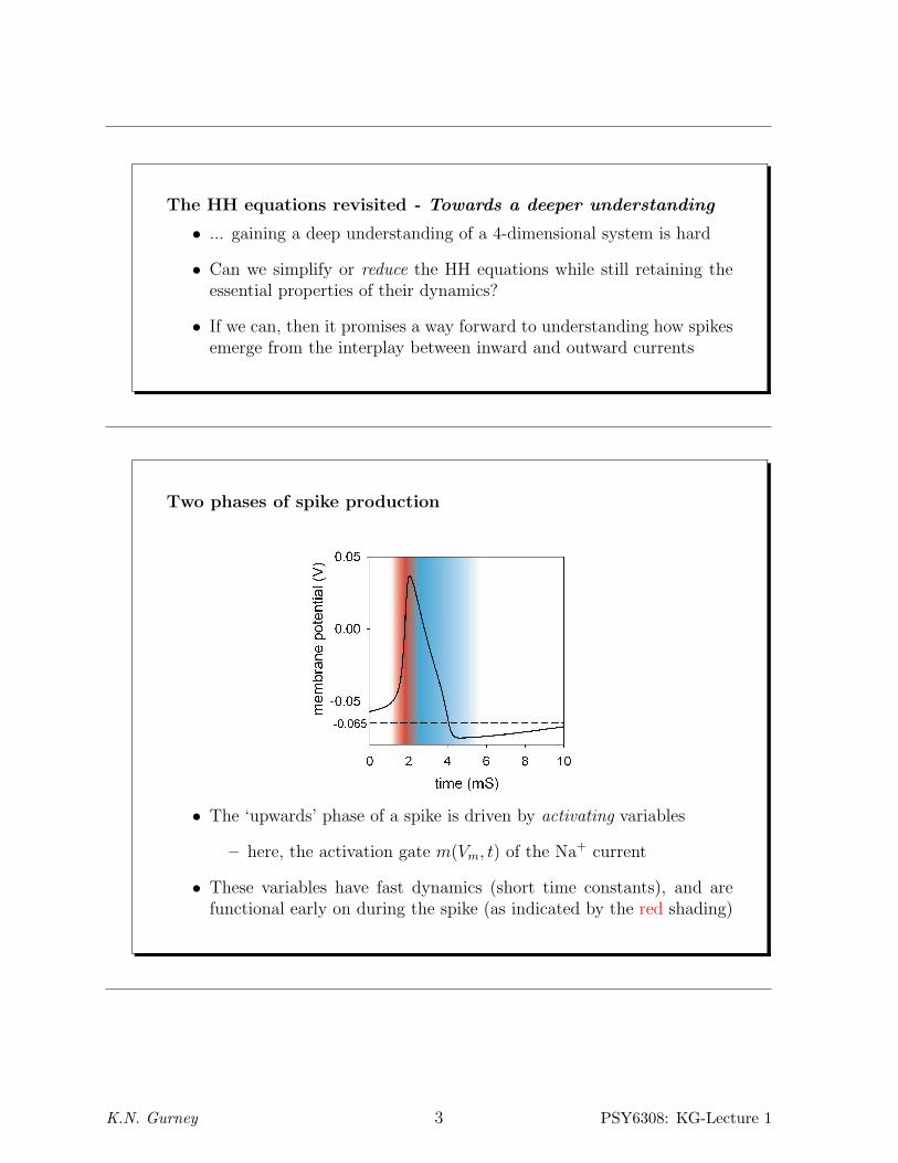
Two phases of spike production

• The ‘upwards’ phase of a spike is driven by activating variables

– here, the activation gate m(Vm, t) of the Na+ current

• These variables have fast dynamics (short time constants), and arefunctional early on during the spike (as indicated by the red shading)


Two phases of spike production

• The membrane is returned to rest (or hyperpolarised) by recovery vari-ables

– here, the inactivation gate h(Vm, t) of the Na+ current, and theactivation gate n(Vm, t) of the K+ current

• These variables have slower dynamics (relatively long time constants)and are functional later on during the spike (as indicated by the blueshading)

Eliminating time dependence of the fast gating variables

• Based on the fast/slow dichotomy outlined above, we make the ap-proximation that the activation variables act instantaneously

• Here, this means m(Vm, t) = m∞(Vm) for all t

• But, because m∞ is a function of Vm only, this means we can eliminatethe separate m variable (and its differential equation) by substitutingthe expression for m∞(Vm) in the membrane equation...


Eliminating time dependence the fast gating variables

CmdVm

dt= gNam∞(Vm)3h(ENa − Vm) (1)

+ gKn4(EK − Vm) + gL(EL − Vm) + Iinj

• The first (Na+ dependent) term is now a complicated function of Vm

but involves no additional variables; we simply use m∞(Vm) as short-hand for the complicated dependence on Vm

Unifying the slow (recovery) gating variables

• The ‘slow’ recovery-phase gating variables h, n are highly correlated:h+ n ≈ 0.83 (red line in plot)

• There is, therefore, only a single independent ‘recovery’ variable

• In fact, their correlation is best fitted with the relation

h+ 1.1n = 0.89 (2)


The graph was obtained by running the Simulink model Reduced_HH.mdl. To controlthis model, you need to interact with the way Na+ works. Double click on the ‘soma’box and then the ‘Fast sodium current’ box (coloured Magenta). The switch (colouredmagenta) allows you to select the use of the full h−gate (as in (1) or the approximationin (2), which results in (3). In all cases, the m−gate is replaced by m∞. You should alsocheck that the injection current is set to 0.2nA by double clicking on the ‘soma input’ boxand setting the first variable in the resulting dialogue box to 2. (While not critical, alsoset the initial membrane potential and n-gate value to −0.065, 0.3185 respectively, usingthe last two text boxes in the dialogue box).

To see the plots shown here, go into the ‘diagnostics’ box and select the gates Kir_actand Naf inact (in the ‘select gates’ box). The difference plot needs to be done ‘offline’by saving the workspace and using the Matlab command line

Reduction of the HH membrane equationSubstitution of (2) in (1) gives

CdV

dt= gNam∞(V )3(0.89− 1.1n)(ENa − V )

+gKn4(EK − V ) + gL(EL − V ) + Iinj

This is augmented with the usual equation describing the dynamics of n

dn

dt=n∞ − n

τn


Comparison with original HH model

Bothmodels driven withIinj = 0.2nA

• Both models produce spikes (no special thresholding required)

• Shape of spikes is very similar in both cases

• Firing rate slightly higher for reduced model

Plots were obtained using the Simulink model Reduced_HH.mdl. In the ‘Fast sodiumcurrent’ box, select the approximation in (2)


Two variable description

Two variable description

• We have reduced the 4-variable HH description to one with only 2variables, V, n

• In general, such 2D models are know as reduced models

• They are predicated on the assumptions that:

– The fast (activation) variables may be ‘lumped’ together into asingle, instantaneous variable (no separate dynamics for this vari-able)

– The slower (recovery or inactivation) variables may be ‘lumped’together into a single, recovery variable whose dynamics are de-scribed by its own equation

• Such models may be explicitly derived from more biologically groundedones (as here), or presented as abstractions of this scheme that obeysimilar dynamics

Taking advantage of the reduction in the variables

• We have worked hard to reduce the 4-variable HH equations to a setwith just two variables

• This allows us to invoke an approach to the analysis of the dynamicswhich is especially powerful

• However, rather than learn about this method in the context of acomplex neural model, we expound it in application to a much simplersystem with which we are familiar


Part II

Phase plane description of dynamicsystems

A simple 2-variable system - The simple pendulum

• We consider as an example, a system about which we have immediatephysical intuition; a simple pendulum swinging back and forth in aplane

• It may be described by two variables:

– The angular displacement θ from the vertical (in degrees)

– The angular speed ω = dθ/dt of the pendulum ‘bob’ around itspoint of suspension (in degrees/second)


The dynamics portrayed in time

• It is common to portray dynamic systems by plotting a key variableagainst time

• In this case we have plotted θ(t)

• The pendulum undergoes a series of damped oscillations before even-tually coming to rest at θ = 0

The plot was generated using the code pendulum.m with a damping force of 1.0 (Matlabvariable ‘force’). Look at the Figure 1 generated in this way.


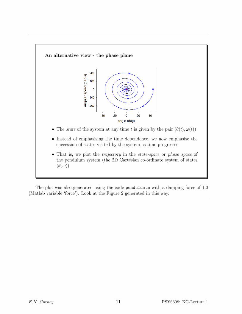
An alternative view - the phase plane

• The state of the system at any time t is given by the pair (θ(t), ω(t))

• Instead of emphasising the time dependence, we now emphasise thesuccession of states visited by the system as time progresses

• That is, we plot the trajectory in the state-space or phase space ofthe pendulum system (the 2D Cartesian co-ordinate system of states(θ, ω))

The plot was also generated using the code pendulum.m with a damping force of 1.0(Matlab variable ‘force’). Look at the Figure 2 generated in this way.


An alternative view - the phase plane

• At t = 0, the system starts at the blue square

• As time advances, the system traverses its trajectory in phase space(direction indicated by the arrows)

• In this view, a damped oscillation corresponds to a ‘spiral’

• The equilibrium state is now explicitly represented (the red circle)


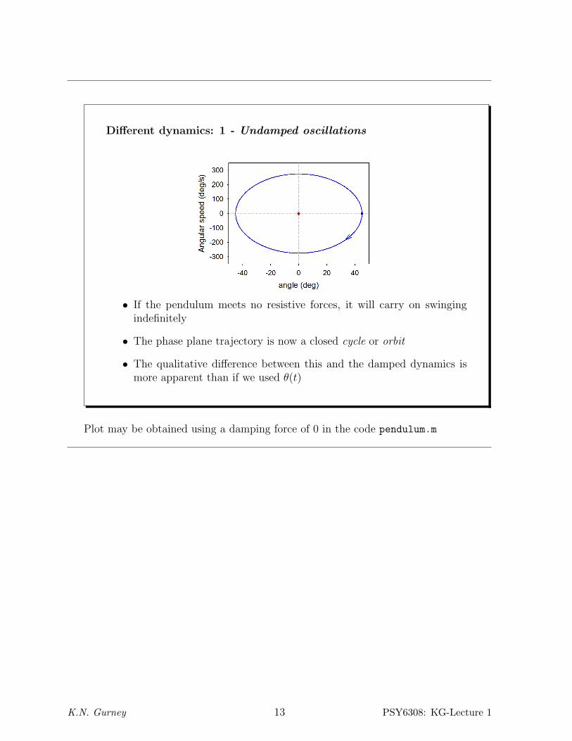
Different dynamics: 1 - Undamped oscillations

• If the pendulum meets no resistive forces, it will carry on swingingindefinitely

• The phase plane trajectory is now a closed cycle or orbit

• The qualitative difference between this and the damped dynamics ismore apparent than if we used θ(t)

Plot may be obtained using a damping force of 0 in the code pendulum.m


Different dynamics: 2 Highly damped oscillations

• If the pendulum meets strong resistive forces, it will barely be able tocomplete a single oscillation

• The phase plane trajectory is a very tight spiral (the time domain plotis shown inset)

Plots may be obtained using a damping force of 6.0 in the code pendulum.m


Why use the phase plane approach?

• The phase plane allows a richer and more immediate graphical por-trayal of the entire dynamics of a system

• The plot opposite shows the vector field for the highly damped pendu-lum

Plot was be obtained using a damping force of 6.0 in the code pendulum.m. Look atthe resulting Figure 4


Why use the phase plane approach?

• It shows the trajectory (dθ/dt, dω/dt) at each point in phase space,and gives an overall picture of the dynamics

• Other insights from the phase-plane approach will occur as we proceed


1 SPIKES IN PHASE SPACE

Part III

Phase plane description of reducedHH model

1 Spikes in phase space

Phase plane view of reduced spiking model - Back to the reducedHH model...

• Because there are only two variables, (n, Vm) , the state of the systemat any time t is described by Vm(t), n(t) and the dynamics may beportrayed in phase space

• uniformly repetitive spiking gives cyclic orbits in phase space

The plot may be obtained by running the Simulink model used previously: Reduced_HH.mdl.Be sure that the initial conditions are those at rest (with no current). Thus, double clickon the ‘soma input’ box to bring up a dialogue box. Then enter −0.065, 0.3185 into the‘Init V’ and ‘Init n’ text boxes respectively (if not already present). The injection currentis 0.2nA.

A an alternative run the m-code !dynamics_HH_reduced. Be sure that the parameters(defined near the top of the file) are set to:

I = 0.2e-9;



do_ramp = 0;

std_noise = 0.0e-10;;

do_reverse_ramp = 1;

reverse_time = 0;

I_start_noise = 1.0e-10;

No_I_pts = 1000;

%% current pulse if required

pulse_time = 0.062;

pulse_width = 0.0005;

pulse_amplitude = 0.0e-10;

% Initial Vm and n-gate value

y0 = [-0.065 0.318];

% duration of simulation in seconds

duration = 0.2;

%% vector field parameters

No_V_steps = 10;

deltaV = 0.0005;

No_n_steps = 10;

deltan = 0.005;

% extent of plotting V-nullcline

lowerV = -0.08;

upperV = 0.06;

Any changes to these will be flagged for later plots that require them.Examine the resulting Figure 2, and ignore for the moment the red and blue lines

(these are the ‘nullclines’ dealt with soon...)



Phase plane view of reduced spiking model

Movie here..

• The movie shows a Matlab ‘comet’ plot of the trajectory during spiking- time is now made explicit again

– Note the axes are not displayed in the movie but are the same asthose on the previous slide


2 FEATURES IN PHASE SPACE

2 Features in phase space

2.1 Equilibria

The resting state

• With Iinj = 0, three initial states of the neuron result in trajectorieswith the same final state - the resting state (V0, n0) of the neuron

• The time dependence of Vm is shown inset for comparison

• In fact, with no input, all trajectories terminate at (V0, n0)

The plots may be obtained by running dynamics_HH_reduced. Put the current to 0,and set the initial conditions as follows: All plots start with the n-gate = 0.4, and thedifferent initial values of Vm are −0.085,−0.058,−0.05. Figure 1 of the simulation givesVm(t)



The resting state

• The resting state is an equilibrium state; starting at (V0, n0), the neuronremains there for all subsequent times

• Note that trajectories 1 and 3 are ‘subthreshold’ PSPs whereas trajec-tory 2 is a single spike



Stability of equilibria - Stable equilibria

• Equilibria may be stable or unstable

• Loosely speaking, an equilibrium (Veq, neq) is stable if nearby trajecto-ries tend to terminate there; small perturbations from (Veq, neq) result(eventually) in the system reaching (Veq, neq) again

• As a non-neural example (in a different state space), think of a ballbearing rolling round a bowl; the centre of the bowl is a stable equi-librium

• The set of states lying on trajectories that terminate (Veq, neq) consti-tute the domain of attraction of (Veq, neq)

Unstable equilibria

• Loosely speaking, an equilibrium (Veq, neq) is unstable if nearby trajec-tories tend to diverge from there; small perturbations from (Veq, neq)result in the system not returning to(Veq, neq) again

– Think of a pencil balanced on its point. The slightest movementcauses the pencil to topple



Phase plane dynamics near stable equilibrium - The vector field

• The diagram shows the vector field of trajectories local to (V0, n0)(green square) with Iinj = 0

• Note its similarity to that for the pendulum; both are centred on anequilibrium known as a stable focus - trajectories tend to ‘spiral in’towards the equilibrium

Plot obtained with code dynamics_HH_reduced.m Make sure the current is zero, andlook at the resulting Figure 4. Start with initial Vm and n at their rest-state values (-0.065, 0.318), or try some of the values used in the previous plots (with n = 0.4) to see aclose up of the process of reaching equilibrium



2.2 Limit cycles

Stable limit cycles

• Recall that when the currents is sufficiently large, the trajectory iseventually cyclic (there are oscillatory ‘spikes’)

• The part of the trajectory that forms a closed loop is a limit cycle

Repeat of earlier plot with Reduced_HH. or dynamics_HH_reduced. Be sure that theinitial conditions are those at rest.



Stable limit cycles

• The limit cycle is shown in red and is stable - that is, nearby trajec-tories are ‘drawn into it’

• The set of states lying on trajectories that converge to points on thelimit cycle constitute its domain of attraction

• Later, we will encounter unstable limit cycles

2.3 Nullclines

The Vm-nullcline

• The Vm-nullcline is the set of points in the plane given by dVm/dt = 0

• It therefore corresponds to solving

gNam∞(V )3(0.89− 1.1n)(ENa − V ) (3)

+ gKn4(EK − V ) + gL(EL − V ) + Iinj = 0

for n as a function of V ; n = n(V )

• In this case, it has to be done numerically



Significance of the Vm-nullcline

• dV/dt = 0 along the nullcline, and dV/dt changes sign across this linein phase space

• Thus, on one side of the nullcline, V is increasing and all trajectoriesmust have a rightward component

• On the other side of the nullcline, V is decreasing and trajectories havea leftward component

Plot is based on Figure 2 obtained when running dynamics_HH_reduced.m. Makesure I = 0.



Significance of the Vm-nullcline

• This is consistent with the trajectory shown earlier

The n-nullcline

• The n-nullcline is the set of points in the plane given by dn/dt = 0

• It therefore corresponds to solving

n∞(V )− n

τn= 0

for n as a function of V

• This is just n = n∞(V ), part of which is shown on the next slide...



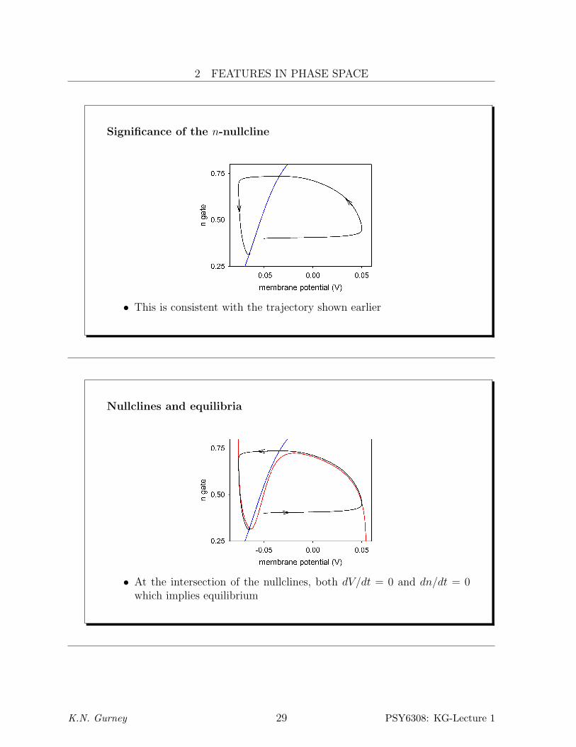
Significance of the n-nullcline

• dn/dt = 0 along the nullcline, and dn/dt changes sign across this linein phase space

• Thus, on one side of the nullcline, n is increasing and all trajectoriesmust have an upward component

• On the other side of the nullcline, n is decreasing and trajectories havea downward component

Plot is based on Figure 2 obtained when running dynamics_HH_reduced.m. Makesure I = 0.



Significance of the n-nullcline

• This is consistent with the trajectory shown earlier

Nullclines and equilibria

• At the intersection of the nullclines, both dV/dt = 0 and dn/dt = 0which implies equilibrium



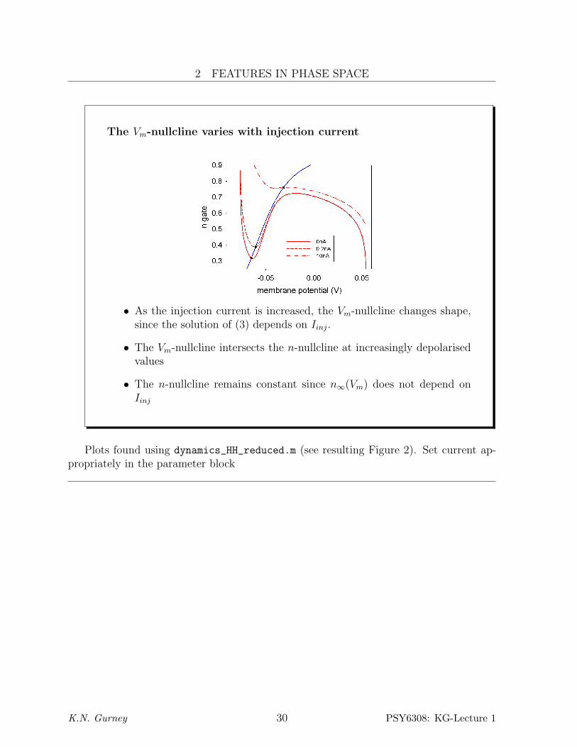
The Vm-nullcline varies with injection current

• As the injection current is increased, the Vm-nullcline changes shape,since the solution of (3) depends on Iinj.

• The Vm-nullcline intersects the n-nullcline at increasingly depolarisedvalues

• The n-nullcline remains constant since n∞(Vm) does not depend onIinj

Plots found using dynamics_HH_reduced.m (see resulting Figure 2). Set current ap-propriately in the parameter block


3 BIFURCATIONS

3 Bifurcations

Qualitative differences in behaviour

• The behaviour under current injection is qualitatively different fromthat when there is no current

– Under current injection there maybe a stable limit cycle in phasespace (we may get spikes)

– With no current, there is no limit cycle and all trajectories ter-minate at the stable equilibrium

• The transitions from one mode of behaviour to the other is know as abifurcation

• We now describe the bifurcations of the reduced HH model in moredetail


3 BIFURCATIONS

Stable focus equilibrium

• For small (or zero) currents, there is a stable focus equilibrium

• The graph shows three trajectories with Iinj = 0

• The inset shows the ‘spiraling in’ to the focus more clearly, and wasreflected in the vector field shown earlier

Plots found using dynamics_HH_reduced.m (see resulting Figure 2). Try differentinitial values of Vm, n obtained by examining the figure here (the exact values are notimportant). Use I = 0


3 BIFURCATIONS

Emergence of stable limit cycles - a bifurcation

• For a sufficiently large current, a new feature appears in the phaseplane: namely a stable limit cycle

Bifurcations

– The appearance or disappearance of a feature in the phase spaceof a system constitutes bifurcation

– The bifurcation is caused by a change in the bifurcation parameter- in our case the injection current

Plots found using dynamics_HH_reduced.m (see resulting Figure 2). Put I = 0.2nA


3 BIFURCATIONS

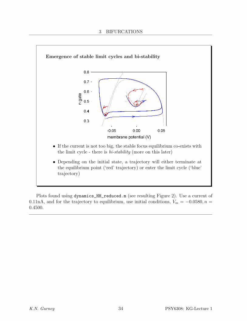
Emergence of stable limit cycles and bi-stability

• If the current is not too big, the stable focus equilibrium co-exists withthe limit cycle - there is bi-stability (more on this later)

• Depending on the initial state, a trajectory will either terminate atthe equilibrium point (‘red’ trajectory) or enter the limit cycle (‘blue’trajectory)

Plots found using dynamics_HH_reduced.m (see resulting Figure 2). Use a current of0.11nA, and for the trajectory to equilibrium, use initial conditions, Vm = −0.0580, n =0.4500.


3 BIFURCATIONS

Unstable limit cycles

• In fact, simultaneous with the emergence of the stable limit cycle, isthe appearance of an unstable limit cycle

• States exactly on this trajectory give trajectories on the limit cycle,whereas states slightly misaligned with it give trajectories that divergefrom the cycle

Since the limit cycle in question is unstable, when the model is run forward in time,trajectories diverge from it. In order to make the cycle visible, we can run the model back-wards in time, by reversing the sign of time in the equations. Run dynamics_HH_reduced.m

with the reverse_time flag set to 1, initial conditions y0 = [-0.06 0.45]; and I =0.114. Look at the resulting Figure 2. In the lecture slide, only a single ‘circuit’ aroundthe cycle is shown. The simulation (with duration of 0.2s) allows several such circuits andit takes a few to converge on the cycle properly.


3 BIFURCATIONS

Unstable limit cycles

• Initial states within the unstable limit cycle will give trajectories ter-minating on the stable focus

• Initial states outside the unstable limit cycle will give trajectories con-verging on the stable limit cycle


3 BIFURCATIONS

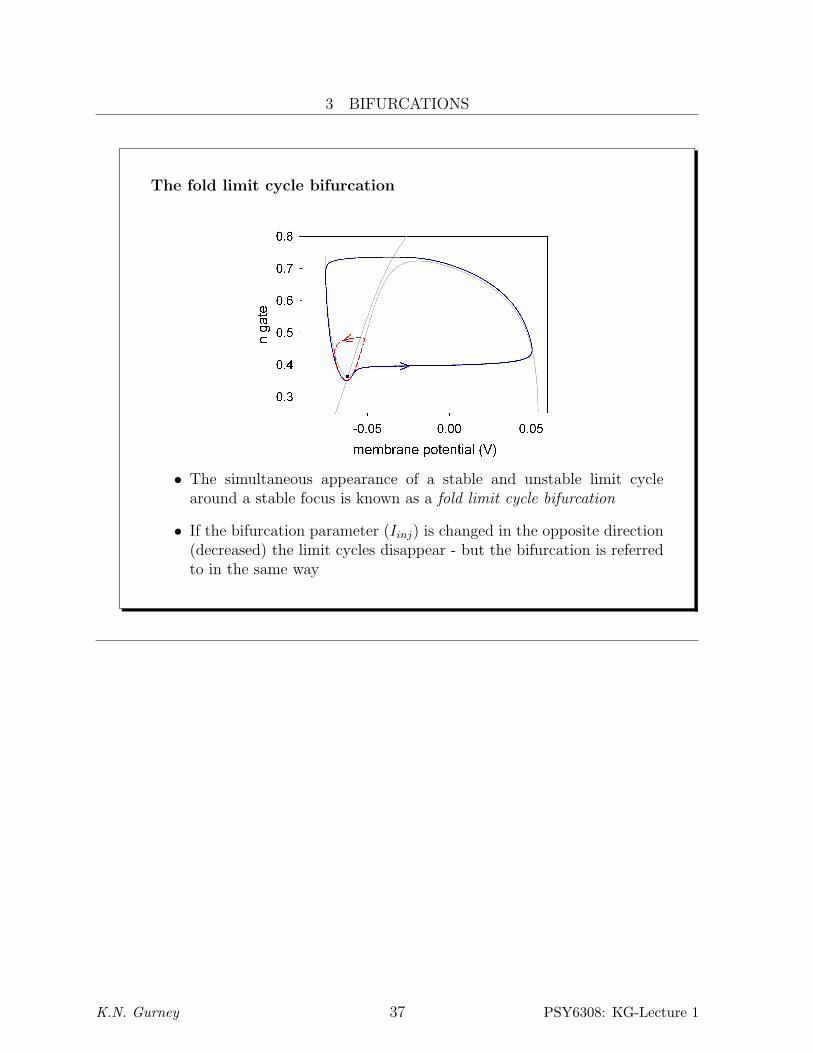
The fold limit cycle bifurcation

• The simultaneous appearance of a stable and unstable limit cyclearound a stable focus is known as a fold limit cycle bifurcation

• If the bifurcation parameter (Iinj) is changed in the opposite direction(decreased) the limit cycles disappear - but the bifurcation is referredto in the same way


3 BIFURCATIONS

The subcritical Andronov-Hopf bifurcation

• As the current is increased still further, the unstable limit cycle shrinks(compare this figure with the previous one)

• Eventually, the unstable limit cycle disappears and, simultaneously,the central focus equilibrium becomes unstable

Run dynamics_HH_reduced.m with the reverse_time flag set to 1, initial conditionsy0 = [-0.06 0.45]; and I = 0.13. Look at the resulting Figure 2.


3 BIFURCATIONS

The subcritical Andronov-Hopf bifurcation

• This constellation of events constitutes a subcritical Andronov-Hopfbifurcation

– sometime Andronov gets no credit and people refer simply to a‘Hopf bifurcation’ !

• Once again, the sequence of events can be traversed in the oppositedirection - but it is still referred to as a subcritical Andronov-Hopfbifurcation


3 BIFURCATIONS

The supercritical Andronov-Hopf bifurcation

• As the current is increased still further, the size of the stable limitcycle becomes ever smaller

Run dynamics_HH_reduced.m with the reverse_time flag set to 0 again. Start fromrest, and put I = 5.0nA and I = 10nA. Look at the resulting Figure 2.


3 BIFURCATIONS


• Eventually, with sufficiently large current (the bifurcation parameter)the stable limit cycle disappears and the unstable equilibrium that wascontained within it, becomes stable

• There is a supercritical Andronov-Hopf bifurcation

Run dynamics_HH_reduced.m and put I = 12nA. Look at the resulting Figure 2.


3 BIFURCATIONS


• The result is that there are no more spikes even though the current isvery large

• This phenomenon is called excitation block and has been observed ex-perimentally


3 BIFURCATIONS

3.1 The bifurcation diagram

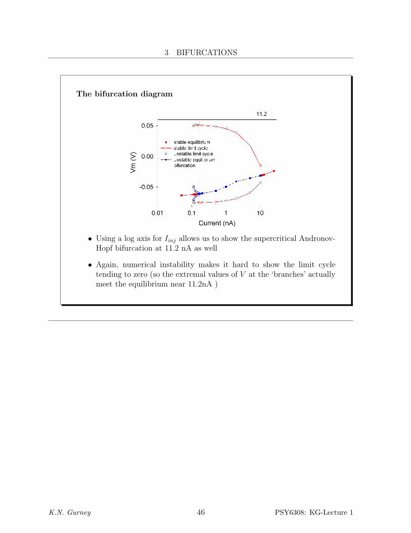
The bifurcation diagram

The data points are from a simulation of the model

• The sequence of bifurcations may be summarised in the bifurcationdiagram

• This is a plot of one of the phase plane variables (in this case V ) againstthe bifurcation parameter (Iinj)

These plots are obtained by running a series of simulations and noting: the maximumand minimum Vm, and the equilibrium values of Vm. These values are reported at thecommand line from dynamics_HH_reduced.m. Careful setting of the current is requirednear the bifurcations.


3 BIFURCATIONS


The data points are from a simulation of the model

• Equilibria are plotted as single points and limit cycles represented bytheir maximum and minimum values

• The fold limit cycle (at 0.113nA), and subcritical Andronov-Hopf bi-furcation (at 0.168nA) are shown


3 BIFURCATIONS


• In fact the stable and unstable limit cycles are initiated from the sameorbit in phase space, but the limits of the numerical simulation preventthat feature being shown for the model itself (the appear to emergewith different trajectories)


3 BIFURCATIONS


• Using a log axis for Iinj allows us to show the supercritical Andronov-Hopf bifurcation at 11.2 nA as well

• Again, numerical instability makes it hard to show the limit cycletending to zero (so the extremal values of V at the ‘branches’ actuallymeet the equilibrium near 11.2nA )


3 BIFURCATIONS

Summary

• The system described by the four Hodgkin Huxley equations for anexcitable membrane can be approximated by, or reduced to, a pair ofequations (4- to 2-variables)

• Therefore, such 2D models are known as reduced models

• Systems with two variable have an immediate graphic portrayal in 2Dphase- or state- space (we used the simple pendulum as an example)

• Phase space has several key features that help describe the dynamics

– Equilibrium states (stable and unstable)

– Limit cycles (stable and unstable)

– Nullclines (divide regions of a variable’s increase/decrease on atrajectory)

– Bifurcations - mark qualitative change in the dynamics

Summary

• The reduced HH model has the following bifurcations with respect tothe injection current as a bifurcation variable:

– A fold limit cycle bifurcation when spiking appears

– A subcritical Andronov-Hopf bifurcation when the equilibriumstate disappears (and only spikes are possible)

– A supercritical Andronov-Hopf bifurcation when spiking disap-pears

• The bifurcation diagram summarise these transitions


3 BIFURCATIONS

Further reading

• The book by Izhikevich (2007) is both comprehensive and readable.Chapter 1 is a good overview, but other chapters, while containingsome mathematics, are well illustrated with plenty of example plots

– I have put up a pdf of an early version of the book on MOLE

• The Chapter by Rinzel and Ermintrout (1998) (in the book edited byKoch & Segev) is a ‘classic’ reference

• The code for all the graphs plotted here is available on MOLE


3 BIFURCATIONS

ReferencesIzhikevich, E. (2007). Dynamical systems in neuroscience: The geometry of excitability and bursting. MIT

Press.Rinzel, J., & Ermintrout, B. (1998). Methods in neuronal modeling: From ions to networks. In (chap.

Analysis of Neural Excitability and Oscillations). MIT Press.

1


single neuron models - kevin...

Documents