Single-Issue Campaigns and Multidimensional Politics∗

Georgy EgorovNorthwestern University

July 2015

Abstract

In most elections, voters care about several issues, but candidates may have to choose only afew on which to build their campaign. The information that voters will get about the politiciandepends on this choice, and it is therefore a strategic one. In this paper, I study a model ofelections where voters care about the candidates’competences (or positions) over two issues, e.g.,the economy and foreign policy, but each candidate may only credibly signal his competence orannounce his position on at most one issue. Voters are assumed to get (weakly) better information ifthe candidates campaign on the same issue rather than on different ones. I show that the first moverwill, in equilibrium, set the agenda for both himself and the opponent if campaigning on a differentissue is uninformative, but otherwise the other candidate may actually be more likely to choosethe other issue. The social (voters’) welfare is a non-monotone function of the informativenessof different-issue campaigns, but in any case the voters are better off if candidates are free topick an issue rather than if an issue is set by exogenous events or by voters. If the first moveris able to reconsider his choice when the follower picks a different issue, then politicians who arevery competent on both issues will switch. If voters have superior information on a politician’scredentials on one of the issues, that politician is more likely to campaign on another issue. Ifvoters care about one issue more than the other, the politicians are more likely to campaign onthe more important issue. If politicians are able to advertise on both issues, at a cost, then themost competent and well-rounded ones will do so. This possibility makes voters better informedand better off, but has an ambiguous effect on politicians’utility. The model and the results mayhelp understand endogenous selection of issues in political campaigns and the dynamics of thesedecisions.

Keywords: Elections, campaigns, issues, dynamics, salience, competence, probabilistic voting,unraveling.

JEL Classification: D72, D82.

∗I am grateful to Daron Acemoglu, Attila Ambrus, Enriqueta Aragonès, David Austen-Smith, V. Bhaskar, ColinCamerer, Timothy Feddersen, Faruk Gul, Matthew Jackson, Patrick Le Bihan, César Martinelli, Joseph McMurray,Mattias Polborn, Maria Socorro Puy, Larry Samuelson, Andrzej Skrzypacz, Konstantin Sonin, and participants ofthe PECA 2012 conference, NES 20th Anniversary Conference, the Econometric Society meeting in Los Angeles in2013, Wallis 2013 Conference in Rochester, Political Institutions Conference in Montreal, ASSA 2015 Conference inBoston, MPSA 2015 Conference in Chicago, Barcelona GSE Summer Forum 2015, and seminars at the University ofBritish Columbia, University College London, Duke University, MIT, New York University, Northwestern University,University of Pennsylvania, and Queen’s University at Belfast for valuable comments and to Ricardo Pique andChristopher Romeo for excellent research assistance.

Campaigns are not like school debates or courtroom disputes. <...>

Campaigns are quite different because there is no judge. Each dis-

putant decides what is relevant, what ought to be responded to, and

what themes to emphasize.

William H. Riker1

1 Introduction

In most elections, voters care about multiple issues and, similarly, parties and individual candidates

write platforms stating their positions on many issues and spanning dozens of pages. Yet, on the

campaign trail, in political advertisements, and in debates, it is typical for candidates to focus on

a narrow subset of issues and reiterate the same points over and over. This strategy makes a lot

of sense if voters pay relatively little attention to the election– for example, if a typical voter will

only see a few ads or attend one rally. The candidates are free to choose their campaign themes,

but the quality and informativeness of the debate may depend on the issues they choose.2 In this

paper, I study informative campaigns with endogenous choice of issues by the candidates.

I assume that voters’preferences are two-dimensional (and separable), and there are two politi-

cians who choose the issues they will run on. Two assumptions are key. First, I assume that a

politician can only credibly announce his position on (at most) one issue, but not on both. The

motivation is that persuading voters about his position or about his talents in a particular area

is hard, and there is only a limited amount of time. If voters’attention is limited, losing focus is

costly for the candidate. In reality, even though candidates occasionally talk about several issues,

the broad idea of the campaign is typically clear: for example, Bill Clinton ran on the economy in

1992, while George H.W. Bush ran on foreign policy; in 1972, George McGovern ran against the

Vietnam war. Sometimes candidates shift their focus during the campaign, as in 2008, when the

financial crisis made the economy– as opposed to foreign policy and, specifically, the Iraq war– the

most salient issue, which subsequently drew the attention of both Barack Obama and John McCain,

or in 2012, when the Romney campaign primarily attacked Obama’s economic record, and Obama

eventually moved from focusing on social issues to defending the economic record of his first term.

Still, the assumption that at each stage (e.g., in a given rally or debate) the candidate adopts a

particular line of attack or defense, which may or may not coincide with the one chosen by his

opponent, seems reasonable.3

1William H. Riker (1993), “Rhetorical Interaction in the Ratification Campaigns,” in Agenda Formation, ed. byWilliam H. Riker. The University of Michigan Press: Ann Arbor, p.83.

2 In a book on candidates’ behavior in American politics, Simon (2002) emphasizes the informational value ofdialogue in political campaigns, but notes that dialogues are rarely observed.

3Campaign advisers have long known the importance of focusing on very few issues and very few talking points.Matalin and Carville (1994) describe the advice they gave Clinton in the 1992 campaign: “Governor Clinton didn’t

1

The second key assumption I make is that voters get better information about a candidate’s

position or competence on a given issue if both candidates choose this issue. In other words, there

is a certain complementarity: a politician sounds more credible if he talks about, say, the economy,

if his opponent talks about the same issue as well. Indeed, the politicians may criticize each other,

check whether the opponent’s factual statements are correct, and thus indirectly add credibility

to each other’s claims. On the other hand, if the opponent talks about another topic, then the

politician’s own credibility is undermined. The process of making statements and having the other

party check their veracity is not modeled in the paper explicitly, but the assumption that voters

learn more if politicians have a sensible debate on the same issue seems natural.4

These two assumptions lead to a simple and tractable model of issue selection. I first study a

basic case where the first mover (termed “Incumbent”for clarity and brevity) commits to building

his campaign on one of the two issues. The other politician (“Challenger”) observes this and decides

whether to reciprocate or talk about the other issue instead. Voters are Bayesian, they update on

the politicians’ decisions and the information that they observe, and vote, probabilistically, for

one of the two candidates. The model gives the following predictions. First, if campaigning on

different issues gives politicians very little credibility, there is a strong unraveling effect, which forces

Challenger to respond to Incumbent and talk about the same issue. However, if a politician is quite

likely to be able to credibly announce his position or establish his competence even when talking

about a different issue, then divergence is possible, and it is in fact more likely that Challenger

will choose a different issue. Second, social welfare (as measured by the expected competence of

the elected politician) does not necessarily increase in the ability of politicians to make credible

announcements when the opponent campaigns on a different issue. The reason is that when this

ability is low, the politicians will choose the same issue in equilibrium, and this will help voters

rather than hurt them. Third, despite loss of information if candidates campaign on different

want to cede any issues to Perot. He said, ‘I’ve been talking about these things [the role of government] for two years,why should I stop talking about them now because Perot is in?’Our response, and it was not easy to confront thegovernor with this, was, ‘There has to be message triage. If you say three things, you don’t say anything. You’ve gotto decide what’s important.’”

4One way to microfound this assumption is by introducing a third-party fact-checker who is active only some ofthe time; however, if both candidates campaign on the same issue, their opponent fills in this role automatically. Thismicrofoundation would be realistic: for example, in 2008, Obama rebutted McCain’s attempt to separate himself fromthe incumbent, George W. Bush, by constantly noting that McCain had voted with Bush 90 percent of the time.An alternative way is to assume that political positions of politicians are correlated, and when one candidate stateshis position, voters update on the other candidate’s position as well. For example, Barack Obama’s open support ofgay marriage might be interpreted as a belief shared by all politicians of his generation and thus have little impacton voters’ decision to support or oppose him– unless his opponent takes a clear stance, too. In this case, again,voters will receive more precise signals about the difference in the candidates’positions when they campaign on thesame issue. Another alternative is to assume that each candidate has a large set of favorable and unfavorable factsand arguments, and if only one politician talks about an issue, the voters only see the facts that favor his position,while if both campaign on an issue, the voters get the full picture (see, for example, Dziuda, 2011, on selective use ofarguments by a biased expert). I do not model either mechanism explicitly in order to focus on the consequences ofendogenous issue selection.

2

issues, fixing an issue for both candidates to campaign on will generally hurt voters. Fourth,

if the first mover (Incumbent) is allowed to reconsider his initial choice of issue (e.g., because

the opponent picked a different issue, or because the campaign is long enough), then switching

focus is not a signal of weakness; rather, it signals competence in both issues. Fifth, if voters

are more informed on Incumbent’s competence in one of the issues, say, the economy, then he is

more likely to campaign on the other issue, on which the voters have less information with respect

to the Incumbent’s level of competence. In practice, this implies that Incumbent is likely to run

for reelection on an issue different than the one with which he had a chance to demonstrate his

competence (or incompetence) during the first term; doing the opposite would be interpreted as a

lack of competence in the other area. Finally, if politicians have some discretion whether to be the

first or second to start a campaign, they will likely postpone a campaign, as this would signal their

relative indifference between the two issues. To the best of my knowledge, this paper is the first to

model the dynamics of issue selection in political campaigns.

Apart from the applied results described above, the model has a theoretical appeal. On the one

hand, despite being parsimonious, with only two individuals making binary decisions, the model

is rich enough to give rise to this broad set of implications which are potentially testable. On the

other hand, for a signaling model with four dimensions of uncertainty (two for each candidate),

the model is surprisingly tractable. It also suggests a novel limitation for the standard unraveling

argument (Grossman and Hart, 1980, Grossman, 1981, Milgrom, 1981), which would be applied to

this model of political campaigns in the following way: if one candidate chose to talk about, say, the

economy, then avoiding this issue would signal the lowest possible competence on this dimension,

and therefore all types, except perhaps the very worst ones, would choose the same dimension. As

this paper shows, this argument may fail if there is an alternative statement that a person can

make; in this case, the benefits of making such a statement may outweight the cost of giving the

wrong perception, and this might destroy the unraveling equilibrium. More generally, this logic is

one of opportunity cost: if disclosing some private information involves an opportunity cost (e.g.,

of time), then the higher this cost (the more valuable the opportunity is), the less unraveling one

can expect.

This reasoning is applicable to one particular aspects of political campaigns: debates. It can

help explain why and when candidates dodge questions in the course of a debate, and why they

often get away with that. This paper suggests the following: if a candidate dodged the question and

proceeded with saying something unimportant, he will be punished severely by the voters. At the

same time, if he made an important statement instead, the voters’opinion about the candidate’s

ability or position regarding the first question will become worse, but only mildly so, and overall,

seizing the opportunity to make an important statement may benefit the candidate. Interestingly,

the better the candidate performs with respect to the other statement he chooses to make, the less

3

the voters will punish him with respect to the original question, as they will believe that dodging

the question was justified.5

The strategic choice of campaign issues by politicians has been the topic of a number of descrip-

tive and formal studies. Riker (1996, see also 1993), in an extensive study of the U.S. Constitution

ratification, observes that politicians are likely to abandon an issue in which they cannot beat their

opponent; this means that debating the same issue should rarely be observed. This observation

predicts “issue ownership”(as in Petrocik, 1996; see also Petrocik et al., 2003; Simon, 2002, con-

tains a model that captures this idea). Aragonès, Castanheira, and Giani (2015) study a model

where parties compete by investing in generating high-quality alternatives to the status quo. Their

model can explain issue ownership whereby parties invest in issues on which they have compara-

tive advantage on; however, if voters are suffi ciently susceptible to priming, “issue stealing”is also

possible. Other papers that model political campaigns as advertisements that raise the salience of

an issue include Amorós and Socorro Puy (2007), which predicts issue convergence if one party has

an absolute advantage on two issues but little comparative advantage, and Colomer and Llavador

(2011), where a challenger proposes an alternative policy on one issue and the incumbent then has

a choice on whether to defend the status quo or campaign on a different issue; the latter paper

predicts issue convergence if voters like the status quo enough, but otherwise divergence is possi-

ble. In Dragu and Fan (2013), politicians need to divide a fixed budget among several issues; the

authors show that more popular parties are likely to campaign and thereby increase the salience of

consensual issues, while less popular parties increase the salience of divisive issues. In Ash, Morelli,

and Van Weelden, campaigning on a divisive issue (“posturing”) signals commitment to a policy

position on that issue but can reduce social welfare because of the neglect of important consensual

issues. Berliant and Konishi (2005) consider candidates who are able to take any positions on any

subset of policy dimensions; they argue that both candidates at least weakly prefer to campaign

on all issues, but this result ceases to hold in the presence of Knightian uncertainty.

The paper most closely related to this one is Polborn and Yi (2006). There, the voters are also

Bayesian and have fixed preferences. The politicians also choose to disclose information on one of

two dimensions: positive information about themselves or negative information about the opponent.

The authors characterize a unique equilibrium, in which running a negative campaign reveals a lack

of positive information about oneself. This paper generalizes Polborn and Yi (2006) for the case5The insights of the paper make it potentially applicable to advertising campaigns. For example, if Apple released

a new iPhone and marketed it with an emphasis on the screen resolution, then Samsung would face a strategic choice.It could advertise the screen resolution of its new Galaxy phone, which would allow potential users to make a directcomparison, or it could advertise the phone’s battery life. The intuition from this paper suggests that either decisionmay be optimal depending on the relative strength of the new device along these two dimensions, and also that theoptimization problems of the first mover (Apple in this example) and the second mover (Samsung) are different. Ofcourse, in the marketing application, another important choice variable is price; however, one can expect the mainintuition to hold. The results may even be directly applicable if the price has to be fixed at some round number, suchas $599 or $699.

4

of generic campaign issues where campaigning on different issues may undermine voters’ability to

learn the truth.6 As it turns out, this generalization removes the complete separability of the two

politicians’problems while preserving tractability; this makes it possible to obtain nontrivial and

realistic predictions about the choice of issues and campaign dynamics.7

The model in this paper assumes that the relevant characteristic of candidates is their compe-

tence in each of the two issues, and all voters have the same preferences (greater competence is

better), but similar forces would be in effect if candidates were competing on more divisive issues; in

the latter case, the counterpart of competence would be the proximity of a candidate’s ideal point

(in a given policy dimension) to the median voter’s position. The model would predict that politi-

cians would have an incentive to campaign on an issue where their position is close to that of the

median voter, and if a politician revealed himself to be distant from the median voter on the issue

he chose, voters would suspect that he is even more radical on the other issue. The results would

be valid under the following assumptions: the candidates cannot commit to any policy position

other than their ideal one in the course of the campaign, and they cannot lie about their position

(or, more precisely, they cannot lie if the other party is campaigning on the same issue and is able

to expose the lie to voters).8 In the current model, voters’preferences are aligned and competence

is unambiguously good, so pandering must take the form of exaggerating one’s competence. The

results are driven by the assumption that doing so is easier if the opponent talks about a different

issue; the assumption that exaggeration is either infinitely costly (or at least that competence is

6Mattes (2007) also considers the possibility of negative campaings and argues that the welfare effect of banningthem would be ambiguous. Several papers study strategic revelation of hard evidence in debates. In Chen andOlszewski (2014), discussants have a choice between strong and weak arguments, and the authors show that commit-ting to a weak argument may sometimes be desirable. In an earlier paper, Austen-Smith (1990) models debates inlegislatures as cheap talk and argues that they affect outcomes only through affecting agenda-setting, but not voting.

7There are several related studies of informative campaigns where voters are Bayesian, but candidates do notface the strategic choice of which issue to campaign on. In Prat (2002), voters observe advertisement spending andview this information as evidence of endorsement by an interest group that provided the campaing finance. In Coate(2004a,b), advertisements transmit information about the candidates’positions on a policy issue (as in this paper,the candidates cannot lie). The amount of advertisements, and thus the number of citizens they cover, is chosenby the candidate and may depend on his political position. Thus, voters who failed to see an advertisement by acandidate infer his political position in a Bayesian way. See also Galeotti and Mattozzi (2011) for a model wherevoters who saw an advertisement may transmit this information along a network.

8There is a large literature on pandering to voters by partisan politicians as well as obscuring one’s positions,both on the campaign trail and in offi ce, starting with Shepsle (1972), who argues that in the presence of voters withlocal risk aversion, equilibria with imperfect revelation of political positions are possible. Alesina and Cukierman(1990) suggest that incumbents have an incentive to be ambiguous (see also Heidhues and Lagerlof, 2003). Glazerand Lohmann assume that maintaining flexibility on an issue, as opposed to committing to a policy, leaves the issuesalient and may therefore benefit the politician. Callander and Wilkie (2007) talk about lying on the campaigntrail, as does Bhattacharya (2011). Kartik and McAfee (2007) consider signaling motive in policy choices; Acemoglu,Egorov, and Sonin (2013) suggest that signaling may make politicians choose policies further from the median voter’sideal point rather than closer to it, thus explaining the phenomenon of populism. Relatedly, Kartik and Van Weelden(2014) show that during campaigns, a politician may reveal himself to be noncongruent as a way to commit to notpandering in the future, or may decide not to do so and leave open the possibility that he is congruent; the campaignsin their paper feature informative cheap talk about politicians’types that nevertheless leaves voters indifferent as towhom to elect.

5

fully revealed) or totally uncontrolled to the point that the candidate has zero credibility makes

the model tractable, but hardly drives the results.9

The rest of the paper is organized as follows. Section 2 introduces the basic model. Section

3 studies the equilibria of the basic model, with sequential or simultaneous moves, and obtains

implications for social welfare and election outcomes. In Section 4, a dynamic version is introduced,

where each politician has a chance to respond to the other’s choice of issue. Section 5 discusses

several extensions of the basic model. Section 6 concludes. Appendix A contains the main proofs;

Appendix B (not for publication, to be made available online) contains auxiliary proofs and treats

some out-of-equilibrium cases.

2 Model

Consider a two-dimensional policy space, one dimension being economy (E) and the other being

foreign policy (F ). There are two politicians, referred to as Incumbent, indexed by i, and Challenger,

indexed by c; this is mainly done for brevity, and otherwise the politicians will be symmetric until

this assumption is relaxed in Section 5.1. Each politician j ∈ i, c has a two-dimensional typeaj = (ej , fj), which corresponds to his ability in economic and foreign policy questions, respectively

(in what follows, a|s will denote the projection of a on issue s ∈ E,F). Consider an electoratewith perfectly aligned preferences: there is a continuum of voters, and the utility of each voter if

politician of type (e, f) is elected is

U (e, f) = e+ f ; (1)

I thus assume that voters weigh both issues equally (this assumption is relaxed in Section 5.2). The

type of each politician j is his private information and is not known to the other politician or voters;

the distribution of types, independent and uniform on Ωj = [0, 1] × [0, 1], is common knowledge.

At the time of voting, all voters have the same information on both Incumbent and Challenger:

they know the history of the candidates’moves as well as the moves of Nature. This information

(or, more precisely, the posterior distribution of (ei, fi, ec, fc) conditional on the history) is denoted

by I for brevity. Voting is probabilistic (see, e.g., Persson and Tabellini, 2000): voter k votes forIncumbent if and only if

E (U (ei, fi)− U (ec, fc) | I) > θ + θk, (2)

9The paper also addresses the question on whether a single political dimension is likely to arise endogenouslyin a multidimensional world. If it is, this would be further justification for studying political competition along asingle dimension, in the same way as Duverger’s law (Riker, 1982; see also Lizzeri and Persico, 2005) justifies studyingpolitical competition between two candidates by predicting the emergence of exactly two candidates in a majoritariansystem. This question is also studied in McMurray (2013); see also Duggan and Martinelli (2011) who study a modelof media slant, where media are assumed to collapse a multidimensional policy position to a one-dimensional one.

6

where θ is a common taste shock and θk is voter k’s individual shock. As is standard, I assume that

θ is distributed uniformly on[− 1

2A ,1

2A

]and θk distributed uniformly on

[− 1

2B ,1

2B

], where A < 1

2

and B < A2A+1 .

During the campaign, each politician can only talk about one issue, economy or foreign policy.

If both talk about the same issue, they have a reasonable conversation or debate, during which the

voters perfectly learn their competences in this dimension (ei and ec, or fi and fc). However, if the

politicians end up campaigning on different issues, the voters find out the politicians’competences

with probability µ only. In other words, a low µ means that it is hard for a politician to make

credible statements without being engaged in a sensible debate with the opponent or, alternatively,

one can think of this as noisy communication between politician and voters when there is nobody

around to limit exaggeration or bluffi ng. In particular, µ = 0 corresponds to zero credibility, and

µ = 1 is the other extreme where a politician’s ability to make credible statements about his

competence does not depend on his opponent’s choice of campaign issue.10 For simplicity, assume

µ > 0; the extreme case µ = 0 is relatively uninteresting, but would require special treatment in

many of the proofs.

More precisely, the types of Incumbent and Challenger are given, respectively, by ai = (ei, fi) ∈Ωi and ac = (ec, fc) ∈ Ωc; they are assumed to be independent and distributed uniformly on their

respective domains, which we for now assume (for simplicity) to be identical: Ωi = Ωc = [0, 1]2.

Incumbent moves first and chooses the issue to campaign on, di ∈ E,F; Challenger observes thisand chooses his issue dc ∈ E,F. In other words, the set of Incumbent’s strategies is Si : Ωi →E,F and the set of Challenger’s strategies is Sc : Ωc × E,F → E,F.11 Nature then decideswhether each of the candidates is successful in announcing his competence, and voters get signals

κi, κc ∈ [0, 1] ∪ ∅ about the politicians’competence on the issues they cover in their campaigns.Thus, if di = dc, then κi = ai|di and κc = ac|dc ; if, however, di 6= dc, then with probability µ voters

get the same signals κi = ai|di and κc = ac|dc , and with probability 1−µ, κi = κc = ∅; let us writeχ = 1 in the first case and χ = 0 in the second.12 Each voter observes the history of moves (di, dc)

and signals (κi, κc), and updates accordingly, thus getting conditional distribution I, which allows10This signal structure may be microfounded in the following way. Assume that a politician may announce any

competence, but is heavily penalized if he is found to have exaggerated. When politicians talk about the same issue,there is only chance µ that some third party is willing to check the politician’s announcements. However, when theytalk about the same issue, there is always someone to do this, and in this case the politicians have to be credible,so voters learn the true competences on this issue. On the other hand, if nobody puts a check on politicians, thenall announce that they are the most competent, and Bayesian voters learn nothing. I do not model this explicitly tosimplify the exposition.11 It should be emphasized that the two candidates do not have private information about the types of their oppo-

nent, and, in particular, Challenger makes his decision knowing the issue that Incumbent chose, but not Incumbent’scompetence in that issue. To put it another way, I assume that politicians have as much information about theiropponents as the voters. This is a simplification of reality, but a helpful one: from a technical standpoint, it preventspoliticians from strategically jamming the opponent’s signal if they know it to be very high.12Alternatively, one could assume that whether κi = ∅ and κc = ∅ is determined independently; this does not

affect the analysis.

7

him to compute the difference in competence between Incumbent and Challenger:

D (di, dc, κi, κc) = E (U (ei, fi)− U (ec, fc) | di, dc, κi, κc) = E (U (ei, fi)− U (ec, fc) | I) . (3)

After that, common shock θ and idiosyncratic shocks θk are realized for each voter k, and voter k

votes for Incumbent if and only if (2) holds.

Both politicians are expected utility maximizers. The utility of each is normalized to 0 if he is not

elected and to 1 if he is elected, and therefore each maximizes the probability of being elected. The

equilibrium concept is the following refinement of the standard Perfect Bayesian equilibrium (PBE)

in pure strategies: voters’beliefs are such that if politician j ∈ i, c (Incumbent or Challenger)chooses E, then his expected utility is nondecreasing in his competence on economy, ej , and if

he chooses F , then it is nondecreasing in fj .13 This simply means that neither politician would

be willing to understate his competence if given this option. In Appendix B, Lemma B2 proves

that monotone PBE must exhibit ‘monotonicity in strategies’: namely, if Incumbent’s strategy

satisfies di (ei, fi) = E for some (ei, fi), then di (e′i, fi) = E for e′i > ei and di (ei, f′i) = E for

f ′i < fi, and similar requirements are satisfied for Challenger’s decisions dc (ec, fc; di = E) and

dc (ec, fc; di = F ), which simplifies the analysis considerably. Finally, I do not distinguish between

equilibria that differ on a subset of types of measure zero; for example, if all incumbents with ei = fi

are indifferent between economy and foreign policy and can choose either way, this is treated as a

single equilibrium.

3 Analysis

In this section, we analyze the game introduced in Section 2. Then, we consider an alternative

story where both candidates choose issues simultaneously. We conclude this Section by studying

social welfare and compare the results for different values of the credibility parameter µ and for

both timings.

Let us first compute the probability of each politician to be elected for any possible posterior

distribution I = I (di, dc, κi, κc). For a given θ, citizen k votes for Incumbent with probability

Pr (θk < D (I)− θ) =1

2+B (D (di, dc, κi, κc)− θ) , (4)

where D (I) is the difference of voters’expectations of the politicians’competences given by (3);

this is is also the share of votes Incumbent gets. Incumbent wins if and only if (4) exceeds 12 , which

happens with probability

Pr (θ < D (I)) =1

2+AD (I) . (5)

13Polborn and Yi (2006) introduce a similar monotonicity refinement in a game where politicians choose to run apositive campaign or a negative campaign. The focus on pure strategies is without loss of generality in the model,but is done to save on notation and to simplify the proofs.

8

Since A is a constant, Incumbent and Challenger seek to maximize and minimize the expectation

of D (I), respectively. They thus solve, respectively,

maxdi E (D (I) | ei, fi) = E (E (U (ei, fi)− U (ec, fc) | I) | ei, fi) and (6)

mindc E (D (I) | ec, fc; di) = E (E (U (ec, fc)− U (ec, fc) | I) | ec, fc; di) , (7)

where the exterior expectations are politicians’at the time of their decision-making, and the interior

ones are voters’.

Let us examine the politicians’problems, (6) and (7), more closely. Notice first that at the

time either politician makes a decision, he knows that he can affect both E (U (ei, fi) | I) and

E (U (ec, fc) | I), i.e., the voters’posteriors both about about himself and about his opponent (e.g.,

Challenger can make a very competent Incumbent appear worse if he chooses a different issue,

because Incumbent may then fail to inform the voters about his competence). However, if he takes

the expectation of voters’posterior regarding his opponent conditional only on the information he

knows at the time of decision-making, he will get the current expectation (both his and the voters’)

of the opponent’s competence, which he cannot change. This greatly simplifies the problem by

effectively separating the problems of Incumbent and Challenger:

Lemma 1 In equilibrium, Incumbent and Challenger maximize, respectively,

maxdiE (E (U (ei, fi) | di, κi) | ei, fi) , (8)

and

maxdcE (E (U (ec, fc) | dc, κc; di) | ec, fc; di) . (9)

Proof. The complete proof of this and other results are in Appendix A.

The properties of equilibrium critically depend on whether µ exceeds 12 or not: for µ > 1

2 ,

unraveling does not happen in equilibrium, whereas for µ ≤ 12 unraveling may happen. The next

Proposition characterizes the equilibrium for a relatively high µ.

Proposition 1 If µ > 12 , there is a unique equilibrium. In this equilibrium, Incumbent chooses

the issue that he is more competent in: economy if ei > fi and foreign policy if fi > ei (and he is

indifferent otherwise). If di = E, then Challenger hooses E if and only if

ec >2µ− 1

2− µ fc + C, where C =4− 5µ+

√µ (8− 7µ)

4 (2− µ), (10)

and if di = F ; then a symmetric formula applies.

9

Figure 1: Challenger’s equilibrium response if Incumbent picked Economy; 12 < µ ≤ 1.

Not surprisingly, Incumbent always chooses the issue that he is most competent in. The Chal-

lenger’s response depends on the chance that he will be understood if he chooses a different issue.

If µ = 1, then his credibility is the same regardless of the issue, and then his strategy is indepen-

dent from the choice of Incumbent: he will always choose the issue his is most competent in. If12 < µ < 1, then he may not be as credible when choosing a different issue. For a very competent (in

both dimensions) Challenger, this gives a reason to choose the same issue as Incumbent, in order

to signal his competence in either issue and avoid being pooled with the less competent mass of

potential challengers. Conversely, if Challenger lacks competence in both dimensions, he is better

off choosing an issue different from Incumbent’s choice, because he will have a better chance to be

viewed as an average rather than a very bad type. In equilibrium, if Incumbent chose Economy,

then the set of Challengers who are indifferent between the two alternatives is a straight line that is

steeper than the diagonal (see Figure 1). In other words, the choice of Challenger is more sensitive

to ec than to fc, which is not surprising since he has a higher chance to communicate ec than fc

credibly. For example, if µ is close to 12 , then Challenger’s choice depends almost exclusively on ec.

We therefore have the following equilibrium strategies of the politicians. Incumbent always

chooses the issue he is best at. Challengers who are good at one issue and bad at the other also

choose their preferred issue, regardless of the choice of Incumbent. However, Challengers which

have roughly equal abilities in both dimensions and who would otherwise be relatively indifferent

respond to Incumbent’s pick of issue in a non-trivial way: those who excel in both dimensions

pick the same issue, whereas very incompetent ones choose a different dimension. The equilibrium

strategies are summarized in Figure 2. Notice that for µ close to 1, the lines separating the four

regions converge to the diagonal, and Challenger’s decision becomes largely independent from that

of Incumbent. Conversely, if µ is close to 12 , the four regions have (almost) equal size, and half of

10

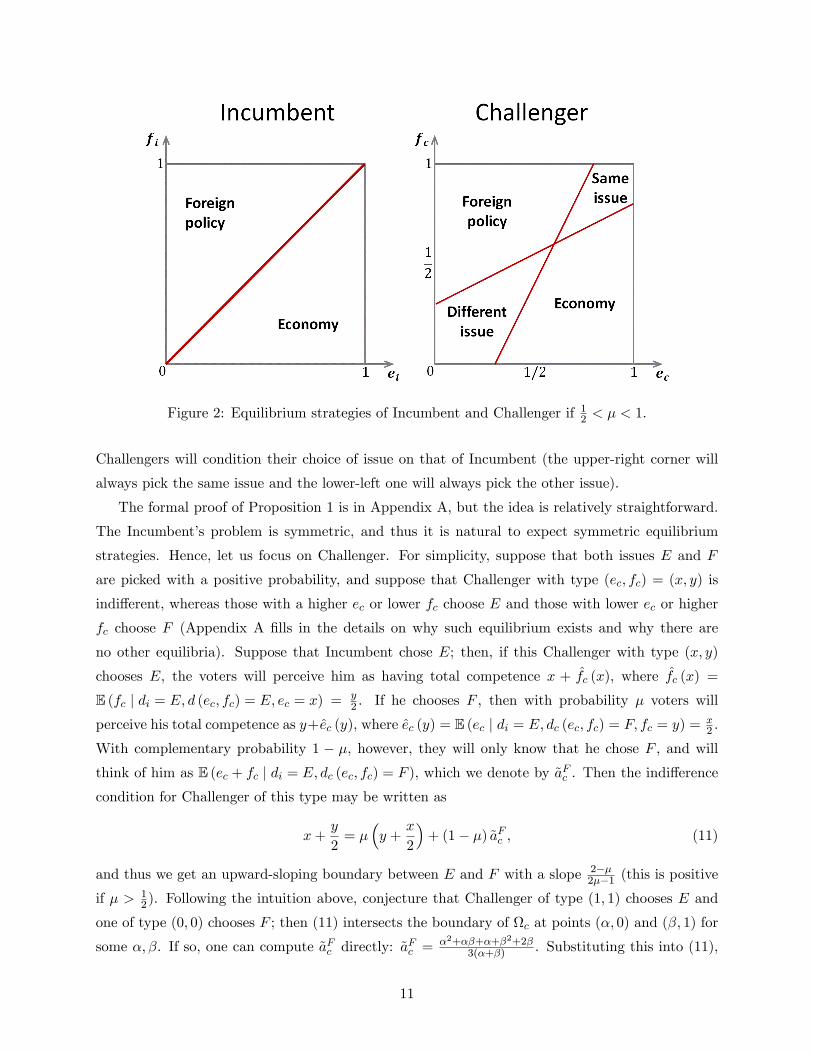
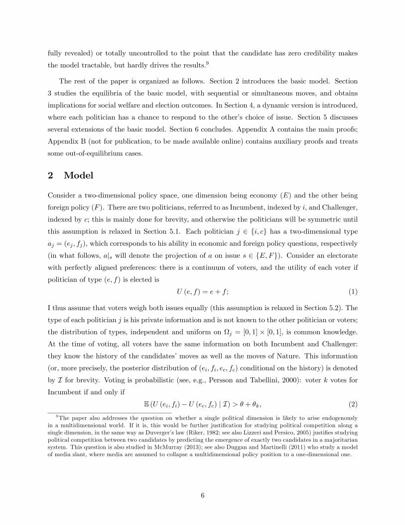
Figure 2: Equilibrium strategies of Incumbent and Challenger if 12 < µ < 1.

Challengers will condition their choice of issue on that of Incumbent (the upper-right corner will

always pick the same issue and the lower-left one will always pick the other issue).

The formal proof of Proposition 1 is in Appendix A, but the idea is relatively straightforward.

The Incumbent’s problem is symmetric, and thus it is natural to expect symmetric equilibrium

strategies. Hence, let us focus on Challenger. For simplicity, suppose that both issues E and F

are picked with a positive probability, and suppose that Challenger with type (ec, fc) = (x, y) is

indifferent, whereas those with a higher ec or lower fc choose E and those with lower ec or higher

fc choose F (Appendix A fills in the details on why such equilibrium exists and why there are

no other equilibria). Suppose that Incumbent chose E; then, if this Challenger with type (x, y)

chooses E, the voters will perceive him as having total competence x + fc (x), where fc (x) =

E (fc | di = E, d (ec, fc) = E, ec = x) = y2 . If he chooses F , then with probability µ voters will

perceive his total competence as y+ec (y), where ec (y) = E (ec | di = E, dc (ec, fc) = F, fc = y) = x2 .

With complementary probability 1 − µ, however, they will only know that he chose F , and will

think of him as E (ec + fc | di = E, dc (ec, fc) = F ), which we denote by aFc . Then the indifference

condition for Challenger of this type may be written as

x+y

2= µ

(y +

x

2

)+ (1− µ) aFc , (11)

and thus we get an upward-sloping boundary between E and F with a slope 2−µ2µ−1 (this is positive

if µ > 12). Following the intuition above, conjecture that Challenger of type (1, 1) chooses E and

one of type (0, 0) chooses F ; then (11) intersects the boundary of Ωc at points (α, 0) and (β, 1) for

some α, β. If so, one can compute aFc directly: aFc = α2+αβ+α+β2+2β

3(α+β) . Substituting this into (11),

11

we have an equation on (x, y) which should hold for (α, 0) and (β, 1). It is then straightforward to

find that α =4−5µ+

√µ(8−7µ)

4(2−µ) , β =3µ+√µ(8−7µ)

4(2−µ) , which implies (10).

Are the two politicians ex ante more likely to campaign on the same issues or on different issues?

Surprisingly, for µ ∈(

12 , 1), the answer is that campainging on different issues is more likely (and

this is captured on Figure 2): Challenger is more likely to choose economy if Incumbent chose

foreign policy, and vice versa. More precisely, we have the following result.

Proposition 2 If µ > 12 , then the probability of having politicians talk about different issues, is

higher than 12 : it increases in µ on

(12 ,

45

)and decreases on

(45 , 1), thus reaching its maximum at

µ = 45 . Nevertheless, the probability that either politician successfully communicates his competence

in the chosen dimension is strictly increasing in µ.

It is true that politicians who choose the opposite issue have lower expected quality, and thus

candidates have an incentive to pool with those who choose the same issue as Incumbent. To get

the intuition for this result, however, consider politicians who are relatively equally competent (or

incompetent) on both issues. Campaigns where one can reveal one’s competence in one issue but not

the other punish such politicians disproportionately harshly, and these types are key to determine

whether Challenger is more likely to choose the same or a different issue. In particular, consider

Challenger of type(

12 ,

12

)and suppose for a second that he is indifferent, which would be true if

campaigning on the same issue was as likely as campaigning on different issues.. If Challenger of

this type reveals his competence in either issue, the voters’posterior beliefs about his competence

will be 12 + 1

4 = 34 . However, it is easy to see that the average competence of politicians choosing

foreign policy if Incumbent chose economy is larger than this (their competence on foreign policy

exceeds 12 , and that on economy exceeds

14), and therefore, as long as µ < 1, the type

(12 ,

12

)would

prefer the opposite issue. Intuitively, politicians who excel in only one dimension are more likely to

be interested in revealing their competence in this dimension, whereas more symmetric politicians

are less interested in communicating credibly and thus are more likely to campaign on a different

issue. The difference reaches its maximum at µ = 45 , where campaigns on different issues are almost

eight percentage points (precisely,√

33 −

12 ≈ 0.077) more likely than campaigns on the same issue.

Why is there no unraveling, i.e., why voters fail to interpret the politician choosing a different

issue as a signal that he is the worst possible type? To see why, consider a candidate equilibrium

where if Incumbent chose E, then all Challengers also choose E, with the out-of-equilibrium beliefs

that if he chooses F , then his ec = 0, and also fc = 0, unless he credibly proves otherwise. Consider

Challenger of type (ec = 0, fc = 1). If he chooses E, he would reveal ec = 0 and nothing on foreign

policy, so the voters’posterior of his total competence will be 0 + 12 = 1

2 . On the other hand, if he

chooses F , then with probability µ he would reveal fc = 1, so voters’posterior will be 1 + 0 = 1;

with probability 1− µ he will reveal nothing and the voters will assume that he is the worst type.

12

In expectation, the voters’posterior will equal µ. Thus, if µ > 12 , then this type of Challenger

would find it optimal to deviate and show his competence on foreign policy to the voters, because,

intuitively, he has a suffi ciently high chance of success. Hence, for such values of µ there is no

equilibrium with unraveling; moreover, once Challengers with types close to (0, 1) start to choose

foreign policy, voters will Bayesian-update and think of Challengers choosing F quite highly, and

then, as Proposition 2 shows, more than half of types will end up choosing F in equilibrium.

If µ ≤ 12 , equation (11) no longer defines an upward-sloping boundary, and thus the equilibrium

must be different. The logic from the previous paragraph suggests that for µ ≤ 12 there should be

equilibrium with unraveling, where each Challenger chooses the same issue as incumbent. As it

turns out, there are other equilibria as well.

Proposition 3 If µ ≤ 12 , then there are multiple equilibria. Incumbent’s strategy is the same

(di = E iff ei > fi) in every symmetric equilibrium. The strategy of Challenger may fall into one

of the two classes:

(i) Challenger always conforms to Incumbent’s choice of issue: dc = di;

(ii) For some cutoff t ∈ [µ, 1− µ]: If Incumbent chose di = E, then Challenger chooses E if

ec > t and chooses F if ec < t (and for ec = t, Challenger chooses E if fc is below the cutoff1−µ−t1−2µ

for µ < 12 and arbitrary cutoff for µ = 1

2); the strategies for di = F are similar.

The equilibrium strategy of Challenger may, therefore, be either to reciprocate Incumbent

or to play a strategy which only depends on his competence in the issue chosen by Incumbent.

If Challenger is expected to play a symmeric strategy (mutatis mutandis) for the two possible

choices of Incumbent, the latter expects that he would be successful in communicating his com-

petence with the same probability regardless of the issue he chooses. In this case, Incumbent

will use a symmetric strategy. In principle, there exist equilibria where Challenger plays very dif-

ferent strategies if Incumbent chose E and F , and then Incumbent must play asymmetrically as

well.14 To avoid these complications, from now on I focus on symmetric equilibria, i.e., equilibria

where the equilibrium play if Incumbent and Challenger have types (ei, fi, ec, fc) = (α, β, γ, δ) and

(ei, fi, ec, fc) = (β, α, δ, γ) will be the opposite.15

To illustrate the equilibria of type (i), suppose Incumbent chose E. If for all (ec, fc),

Challenger chooses E, then E (fc | di = E, d (ec, fc) = E, ec = x) = 12 for all x; at the same

14For example, suppose µ = 14, then there is an equilibrium where all Incumbents choose E; if that happened,

Challenger also chooses E, but if Incumbent chose F , Challenger picks E if and only if fc < 34. In terms of Proposition

3, Challenger plays type (i) equilibrium if di = E and type (ii) equilibrium if di = F . From Incumbent’s perspective,he is able to signal his competence with probability 1 if he chooses E, and with probability 1

4+ 3

4µ = 7

16< 1

2if he

chooses F ; in this case it is an equilibrium for all incumbents to choose E (effectively, he has the same incentives aChallenger would have if µ = 7

16< 1

2).

15There are many alternative ways to define the same restriction. E.g., it would be suffi cient to assume that thechances of Incumbents (Challengers) with type (x, y) and with type (y, x) to be elected are the same. It is remarkablethat for µ > 1

2, such symmetry need not be assumed, but may rather be proved (see Proposition 1).

13

time, ec (y) = E (ec | di = E, dc (ec, fc) = F, fc = y) may be chosen arbitrarily, as may aFc =

E (ec + fc | di = E, dc (ec, fc) = F ). If Challenger of type (x, y) chooses E, voters believe his com-

petence is x+ 12 , and if he chooses F , they believe it is µ (y + ec (y)) + (1− µ) aFc . Clearly, the type

most likely to deviate is (x, y) = (0, 1); Challenger of this type does not deviate if and only if

1

2≥ µ (1 + ec (1)) + (1− µ) aFc .

Since ec (y) , aFc ≥ 0, such equilibrium is possible only if µ ≤ 12 . At the same time, for such values

of µ, it is indeed an equilibrium; it suffi ces to set ec (y) = 0 for all y and aFc = 0.

Equilibria of type (ii) are also possible only if µ ≤ 12 . Indeed, fix t and consider the strategies

in Proposition 3 (ii). Then fc (x) = E (fc | di = E, d (ec, fc) = E, ec = x) equals 12 if x > t, and may

be chosen arbitrarily if x < t. At the same time, E (ec | di = E, dc (ec, fc) = F, fc = y) = t2 for all y;

we also have E (ec + fc | di = E, dc (ec, fc) = F ) = t2 + 1

2 . To verify whether threshold t constitutes

an equilibrium, it suffi ces to concentrate on the types most likely to deviate. In equilibrium, type

(t+ ε, 1) must prefer E and type (t− ε, 0) must prefer F ; this yields two conditions:

t+ ε+1

2≥ µ

(1 +

t

2

)+ (1− µ)

(t

2+

1

2

),

t− ε+ fc (t− ε) ≤ µ

(0 +

t

2

)+ (1− µ)

(t

2+

1

2

).

Since these conditions need to hold for ε arbitrarily close to 0, the first condition implies t ≥ µ,

whereas the second one (setting fc (t− ε) = 0) implies t ≤ 1−µ. It is now straightforward to showthat Challengers with ec 6= t do not have incentives to deviate. Showing that Challengers with

ec = t have no deviations is also straightforward and is done in the Appendix.

In Subsection 3.2, voters’welfare is computed under different equilibria and parameter values,

and it turns out that if µ ≤ 12 , the unraveling equilibrium, i.e., the equilibrium of type (i) dominates

every equilibrium of type (ii) in terms of welfare.16 The reason for this is that the two politicians

always campaign on the same issue, and a low µ does not result in loss of information due to

their campaigns lacking credibility. The equilibrium of type (i) is unique for any µ, and thus this

equilibrium refinement extends the uniqueness result from Proposition 1 to the case µ ≤ 12 . This

is the equilibrium we focus on from now on.

3.1 Simultaneous game

Consider an alternative game, where the two politicians must choose their campaign issues simul-

taneously (or, equivalently, Challenger starts his campaign before he gets a chance to observe the

choice of Incumbent). Consider exactly the same game as the one introduced in Section 2, except

that Challenger, when deciding on dc, does not observe the choice of Incumbent, di.

16The asymmetric equilibria, such as the one in Footnote 14, are also dominated by the unraveling equilibrium.

14

Given the symmetry of the game, it is not surprising that there is a symmetric equilibrium,

where each politician j picks dj (ej , fj) = E if ej > fj and dj (ej , fj) = F if ej < fj . Indeed,

for either politician, the probability of ending up campaigning on the same issue as the opponent

is exactly 12 and this does not depend on the issue; this means that each politician is able to

send a credible signal with probability 12 + µ

2 , regardless of the issue he chooses. Consequently, if

one politician follows this symmetric strategy, then the other one also must do so in equilibrium.

Hence, symmetric strategies by the politicians are “best responses”to one another, and thus such

an equilibrium exists for all µ.

Proposition 4 For any µ there exists a symmetric equilibrium where each politician j ∈ i, cchooses dj (ej , fj) = E if ej > fj and dj (ej , fj) = F if ej < fj. Moreover, if µ > 1

2 , this is the

unique equilibrium.

This proposition does not preclude existence of equilibria which are not symmetric in the two

issues: for example if µ ≤ 12 , then there is an equilibrium where di (ei, fi) = dc (ec, fc) = E for both

politicians and all types. Indeed, Proposition 3 implies that that if Incumbent plays E, it is an

equilibrium for all Challengers to pick E regardless of their type; if the moves are simultaneous,

then the opposite is also true: if all Challengers are expected to pick E, it is an equilibrium for all

Incumbents to do so as well.17 However, for µ > 12 , only symmetric equilibria exist.

3.2 Social welfare

In this subsection, we study the consequences of the issue selection game on social welfare and

provide comparative statics results. For the society, the relevant variable is the expected competence

of the elected politician. The following lemma shows that in the probabilistic voting model as

above, there is a simple formula for this expected competence. This formula applies to sequential

and simultaneous games as well as some other situations (only players’stragegies matter, but not

whether they form an equilibrium in a specific game played by the politicians), and we use it

throughout.

Lemma 2 Let I (ei, fi, ec, fc, χ) be the voters’posterior beliefs about the distribution of the skills

of the two politicians, (ei, fi) , (ec, fc) ∈ Ωi × Ωc, that voters will get if these politicians follow the

equilibrium play and χ denotes Nature’s choice to reveal competences if di 6= dc.18 The expected

17For µ ∈(

15, 1

2

], there are only three equilibria, up to measure zero: the symmetric one; all types of Incumbent

and Challenger choose E, and all choose F . For µ ≤ 15, more exotic equilibria are possible as well. For example, if

µ ≤ 15, there is an equilibrium where each politician j campaigns on E whenever ej ≥ 1

4and on F otherwise.

18This is a slight abuse of notation, as we previously used I to denote the posterior distribution conditional onpoliticians’choices and information obtained by voters, I (di, dc, κi, κc). However, since in a pure strategy equilibrium,the tuple (ei, fi, ec, fc, χ) predicts (di, dc, κi, κc) uniquely, then I (ei, fi, ec, fc, χ) is well-defined.

15

quality of the elected politician equals

1 +A

∑χ∈0,1

µ if χ = 1

1− µ if χ = 0

∫Ωi×Ωc

([E (U (ei, fi) | I (· · · ))]2

+ [E (U (ec, fc) | I (· · · ))]2)dλ− 2

, (12)

where λ is the standard Lebesgue measure on Ωi × Ωc.

Proof. Fix either of the realizations of χ. Following equilibrium play of politicians, the expected

competence of the elected politician equals (dropping the argument at I for brevity):∫Ωi×Ωc

( (12 +AE (U (ei, fi)− U (ec, fc) | I)

)E (U (ei, fi) | I)

+(

12 −AE (U (ei, fi)− U (ec, fc) | I)

)E (U (ec, fc) | I)

)dλ

= 1 +A

∫Ωi×Ωc

[E (U (ei, fi) | I)− E (U (ec, fc) | I)]2 dλ.

The result (12) would follow immediately (by opening the brackets and taking the weighted sum

over the realizations of χ) if the expected utilities inside the last integral were independent. They

are not; for example, a high realization of E (U (ei, fi) | I) means that most likely the politicians are

talking about the same issue, and, therefore, Challenger is likely to have high average competence.

However, conditional on the choices of issues by both politicians, these variables are independent.

In addition, the choice of issue by one politician does not depend on the competence of the other

one, except through the choice of issue, even if the case of sequential moves. This implies that

social welfare may be computed using (12). Appendix A fills in the details.

Lemma 2 simplifies the computations considerably. In particular, it shows that the expected

competence of the elected politician only depends on the sum of variances of posterior beliefs that

politicians’equilibrium play generates. This allows to do the computations for Incumbent and Chal-

lenger separately, only taking into account the equilibrium strategies. Interestingly, formula (12)

shows that voters’welfare increases in the variance of their posterior beliefs about each politician’s

total competence. This is intuitive; it means that a more informative campaign, which generates

more heterogenous beliefs, results in higher welfare than a less informative one, where posteriors

might be not that different from the priors.

In evaluating the welfare consequences, the following benchmarks are useful. First, if the winner

were picked at random, the average competence would be the unconditional expectation, i.e., 1. At

the opposite extreme is the full information case: if both candidates revealed their competences to

voters on both dimensions, then the expected quality of the winner would be

1 +A

(2

∫ 1

0

∫ 1

0(x+ y)2 dxdy − 2

)= 1 +

1

3A. (13)

Thus, 13A is the extra benefit of having elections as opposed to picking the candidate randomly;

this is the maximum one can achieve with probabilistic voting where a less competent candidate

16

has a chance due to a shock to preferences θ. As the variance of the common shock decreases (A

becomes higher), the expected competence of the elected politician would increase.

In the case of sequential voting, we have the following result.

Proposition 5 The expected competence of the elected politician is increasing in A. It is non-

monotone in µ; more precisely, it equals 1 + 524A if µ ≤

12 (if type (i) equilibrium from Proposition

3, which yields the highest social welfare among all equilibria, is played), and for µ > 12 , it monoton-

ically increases from 1 + 316A < 1 + 5

24A to 1 + 14A > 1 + 5

24A.

The nonmonotonicity result is not surprising if one takes into account that for µ < 12 , the

two politicians are guaranteed to discuss the same issue (in the welfare-maximizing equilibrium),

whereas for µ slightly exceeding 12 such equilibrium does not exist, and the politicians will talk

about different issues at least half of the time (even more than that, as follows from Proposition

2), and thus there is a chance of about one-fourth that they will fail to announce their respective

competences. In fact, the expected competence exceeds 1 + 524A only if µ > 0.7. In all cases, this

falls short of the maximal possible gain of 13A, although if µ is close to 1, then 75% of this gain is

realized, and even in the worst-case scenario this chance exceeds 56% ( 916).

Consider now the welfare implications of a game where strategies are chosen simultaneously.

Proposition 4 established that a symmetric equilibrium exists for all µ, and arguably it is the most

plausible one (and unique if µ > 12). We get the following comparison in this case.

Proposition 6 In the symmetric equilibrium of the game with simultaneous moves, the expected

quality of the elected politician equals 1 + 1+µ8 A; this is lower than the expected quality in the game

of sequential moves if µ ≤ 12 , but it is higher than that if

12 < µ < 1.

The intuition for this result is simple: all things equal, voters make a more informed choice,

and therefore get a higher utility, if politicians reveal more information about their competences.

This is more likely to happen (again, all things equal) if µ is high, and given that the strategies

are the same, the expected quality is increasing in µ. The probability of campaigning on the same

issue in the game with simultaneous moves is 12 ; on the other hand, Proposition 2 states that in the

game with sequential moves, it is less than 12 for µ ∈

(12 , 1). This explains higher voter welfare for

such µ in simultaneous game. If µ ≤ 12 , then sequential moves allow politicians to converge on the

same issue and have an informative discussion at least on that issue. With simultaneous moves,

they lack the ability to converge, and thus the welfare of voters is lower in this case.

If there is a concern that social welfare is lower if politicians fail to coordinate on the same

issue, then one alternative would be to choose an issue (say, at random), and then require that

both politicians campaign on that issue. Formula (12) applies to this case as well, and the expected

17

quality of the winner equals

1 +A

(2

∫ 1

0

∫ 1

0

(x+

1

2

)2

dxdy − 2

)= 1 +

1

6A (14)

(indeed, if a politician announces competence x on one dimension, the voters expect his total

competence to be x+ 12). Comparing this result to Proposition 5 reveals that for all µ, the expected

competence in the case where politicians are free to choose their issue is higher than if they are

not. This seems surprising, because if the issue is fixed, there is no loss due to possible failure to

announce their competences credibly in any dimension. However, there is a different force at play:

with endogenous choice of issues, the announcement of a politician of his competence over one issue

carries quite a bit of information about his competence on the other issue, which is not the case if

they were forced to talk on a given issue (this is true for Incumbent for any µ, and for Challenger

if µ > 12). It turns out that the latter effect dominates.

19

Proposition 7 If politicians were forced to campaign on an exogenously chosen dimension, then

for all values of µ, social welfare would be strictly lower than in the game of sequential moves. It

would be lower than in the game with simultaneous moves as well (if the symmetric equilibrium

is played), provided that µ > 13 ; if, however, µ < 1

3 , then forcing politicians to campaign on an

exogenously given dimension results in a higher social welfare than a simultaneous-move game.

Figure 3 illustrates the expected qualities of elected politicians under different scenarios. Propo-

sition 7 suggests that the only scenario where allowing politicians to choose issues hurts welfare is

when this choice is simultaneous (so the politicians do not coordinate), and also µ is suffi ciently

low, so voters often fail to get precise information about candidates’competences.20 This leads to

the following nontrivial observation. When candidates choose an agenda for an entire campaign,

the decisions are unlikely to be made at once, and hence constraining the candidates by imposing

an issue on them is not a good idea. However, when it comes to some particular event, such as a

debate, where candidates are likely to prepare their communication strategy without observing the

opponent’s plan, fixing a particular issue may make sense. Notice that for µ ∈(

12 , 1), it is better for

voters if politicians made their campaign decisions independently; indeed, with sequential decisions,

19 In Subsection 5.2, we consider the case where issues have different weights. It turns out that allowing politiciansto choose issues freely is still optimal: even though the voters would prefer that the politicians compete on themore important issue, they would do that in equilibrium anyway. We show this result formally for µ = 1; in thesequential game, numerical simulations confirm this hypothesis for other values of µ as well. However, for more generaldistributions of types this is not necessarily true: for example, if the competence of Challenger over one dimensionis very uncertain and µ < 1, the society would strongly prefer Incumbent to choose that issue, but Incumbent wouldordinarily do that with probability 1/2 only.20Caselli and Morelli (2004) and Mattozzi and Merlo (2007) consider very different models that lead to selection

of incompetent politicians. In this paper, incompetent politicians may get elected because voters do not necessarilymake a strong inference about a politician’s incompetence in the issue he is not campaigning on.

18

Figure 3: Social welfare under different scenarios and values of µ.

it is more likely that they will campaign on different issues, while with independent decisions this

probability is fixed at 12 .

3.3 Probability of being elected

Another natural question is whether the timing of the game gives an advantage to Incumbent or

Challenger. At first glance, the sequential timing allows Incumbent to pick the issue that he prefers,

and thus can guarantee that he will talk about the issue that he excels at. However, the voters

are aware of this strategy, and discount Incumbent’s competence on the other issue accordingly.

Challenger, on the other hand, does not have such flexibility, and if µ < 12 he is compelled to choose

the same issue as Incumbent, which might not be his strong side. The voters understand this, and

do not infer Challenger’s competence in the other dimension from his announcement, and thus if

Challenger turns out to be incompetent in the issue that Incumbent picked, he is not penalized

further. In other words, Incumbent has a higher chance to establish his high competence, but if he

fails to do so, he will be perceived as very incompetent; in contrast, the variance of voters’posterior

beliefs about Challenger is likely to be smaller. In the probabilistic voting model, however, it is

the voters’posterior expectations of the politicians’competences that matter, and they are equal

for the two politicians as long as they are taken from the same distribution. This implies, for

example, that before knowing his type, a politician is indifferent between being the first-mover and

19

the second-mover in the game.

Proposition 8 The probability of Incumbent winning and Challenger winning are equal.

At the same time, a given type of politician need not be indifferent. For example, if µ < 1, then

all politicians who are equally competent on both dimensions, with ej = fj < 1, would prefer to

be second-movers rather than first-movers. In Subsection 5.4, Incumbent will be given an option

to postpone his announcement and allow Challenger to move first. It turns out that while not all

types of Incumbent will use this option, those who do are likely to be competent, and this will

result in observable first-mover advantage.21

4 Dynamics of campaign

In this Section, I extend the baseline model by allowing the Incumbent (who moves first) to re-

consider his initial choice if the Challenger chose a different issue. The idea here is to capture the

process of finding a common theme for the campaign or debates and to make sure that both players

have an opportunity to respond to the opponent’s suggestion. Specifically, consider the following

timing. As before, Incumbent moves first and picks a (now tentative) issue for his campaign, di.

Challenger observes this choice and responds with his own (final) decision dc. If the two issues

coincide, di = dc, then the parties proceed to campaigning on this issue, and so Incumbent’s final

decision is di = di. If, however, di 6= dc, then with some probability p, Incumbent has an oppor-

tunity to revise his initial decision, and is free to pick any di ∈di, dc

= E,F, and with a

complementary probability 1 − p he has to stick to di = di. The probability p may correspond to

the chance that the Incumbent’s campaign team is flexible enough or has enough time to switch the

focus.22 This timing (as well as a possible conversation) is shown on Figure 4.23 I assume that vot-

ers observe the entire sequence of moves(di, dc, di

); in particular, they know whether Incumbent

was the first to propose the issue of his campaign di, or he started with a different issue and then

switched. In what follows, restrict attention to symmetric equilibria, which implies, in particular,

that the first proposal by Incumbent is di = E if ei > fi and di = F otherwise. To ensure existence

21 In Ashworth and Bueno de Mesquita (2008), incumbency advantage arises in a probabilistic voting model dueto his ex-ante higher competence (which in turn is present because he had won elections before). Since this paperassumes, for simplicity, that the candidates are ex-ante symmetric, this effect is not present.22Alternatively, one can think of p as the share of voters who get Incumbent’s message after he switches, and 1− p

is then the share of voters who pay attention at the beginning of the campaign only. Probabilistic voting ensuresthat these two interpretations are equivalent.23 If Incumbent were allowed to revise his initial pick even if Challenger chose the same issue, then the first-stage

announcement by Incumbent would have to involve “babbling”. The reason is that in a candidate equilibrium wherefirst announcement is informative, switching to another issue should be interpreted as competence in both issues.Thus, it would make sense to announce the weaker issue for at least some types, and this cannot be true in equilibrium.I am indebted to V. Bhaskar for the suggestion to explore the possibility that Incumbent must stick to his originalchoice if Challenger approves the choice of issue.

20

Figure 4: Timing of proposal-making by Incumbent and Challenger in the dynamic game.

of such equilibria, assume that p is not too close to 1 (precisely, we need p ≤ 4√

3− 6 ≈ 0.93);24 to

avoid issues with multiplicity, assume µ > 12 .

Let us focus on Incumbent’s second choice on whether to switch the campaign issue; this question

is relevant only if dc 6= di. For concreteness, suppose di = E and dc = F . In this case, Incumbent

may either agree to discuss foreign policy or insist on talking about economy. Suppose first that

Incumbent is very competent in economy but not in foreign policy, for example, his type is (1, 0).

For such Incumbent, switching to foreign policy is unlikely to do him any good: indeed, he would

have a (weakly) higher chance to signal his competence credibly, but the signal will be about his

much weaker dimension, foreign policy, and this is precisely what he prefers to avoid. In contrast,

suppose that Incumbent is very competent in both dimensions, say, type (1, 1− ε). In this case, itmakes perfect sense to comply with Challenger’s proposal and switch to foreign policy. By doing

so, not only he will be able to signal that he is highly competent in foreign policy; in addition,

voters will take into account that foreign policy is his weaker issue, and therefore he must be even

more competent in economy (which he truly is). For such Incumbent, therefore, switching allows

to signal competence in both dimensions, which is otherwise diffi cult to achieve. If he insisted

in talking about economy, he would, with some probability, reveal his highest competence in this

issue, but voters would view his foreign policy credentials to be average at best (and, in fact, worse

than average, because they expect those who excel in foreign policy to switch). Therefore, one can

expect that in equilibrium Incumbent will insist on campaigning on the issue he originally chose if

24The reason why existence may fail if p is too close to 1 is the following. Consider Incumbent who is very competentin both issues, but slightly better at E (e.g., type (1, 1− ε)), and suppose he chooses di = E at first. From Proposition2, we know that if µ > 1

2, Challenger will pick dc = F with probability higher than 1

2; it turns out that this remains

true in this version of the game as well (in fact, the possibility of Incumbent switching increases Challenger’s chance ofconveying his competence, and increases the ‘effective µ.’But this would imply that very competent Incumbents who,as we will see, are always willing to switch to signal their competence on both issues, expect to end up talking about Fwith a higher probability than about E. But if he switched to F , he would, similarly, end up campaigning on E witha higher probability, which he prefers. This leads to nonexistence of a monotone equilibrium in pure strategies. Onthe other hand, if p ≤ 4

√3−6, then the probability of talking about E upon choosing di = E equals (1− p)+pz ≥ 1

2,

which ensures that monotone strategies form an equilibrium (here, z = 12− 1

2

(√3

3− 1

2

)= 3

4− 1

6

√3 ≈ 0.46 is the

smallest probability that Challenger will choose the same issue as Incumbent).

21

his competence in the other issue is low, but will be open to switching if he is competent on the

other issue as well.

What is the choice of Challenger who received a proposal to talk about, say, economy, and

anticipates that if he proposes foreign policy instead, then Incumbent will follow the strategy above?

Such Challenger knows that if he agrees on E, then both will campaign on economy, and his signal

will be credible with probability 1. At the same time, if he chooses F instead, he will talk about F ,

but will only be able to send a credible signal with probability µ′ = pη + ((1− p) + p (1− η))µ =

µ+ pη (1− µ), where η is the probability of Incumbent switching to F if given such chance. Since

we assumed µ > 12 , we are guaranteed to have µ

′ ≥ µ > 12 , and therefore the characterization of

Challenger’s strategies from Proposition 1 applies (with µ replaced by µ′). It remains to verify that

Incumbent’s strategy to start with the issue he is most competent in is indeed an equilibrium; one

can verify that this is true if p is not too close to 1, as we assumed. We therefore have the following

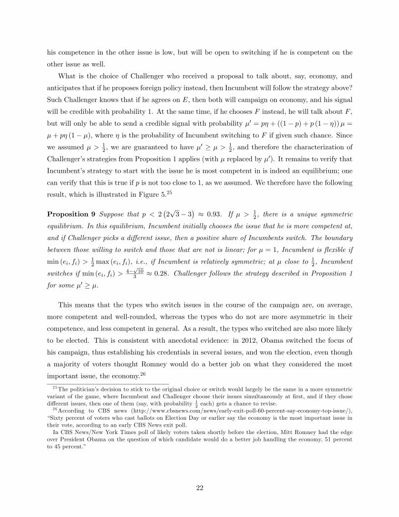
result, which is illustrated in Figure 5.25

Proposition 9 Suppose that p < 2(2√

3− 3)≈ 0.93. If µ > 1

2 , there is a unique symmetric

equilibrium. In this equilibrium, Incumbent initially chooses the issue that he is more competent at,

and if Challenger picks a different issue, then a positive share of Incumbents switch. The boundary

between those willing to switch and those that are not is linear; for µ = 1, Incumbent is flexible if

min (ei, fi) >12 max (ei, fi), i.e., if Incumbent is relatively symmetric; at µ close to 1

2 , Incumbent

switches if min (ei, fi) >4−√

103 ≈ 0.28. Challenger follows the strategy described in Proposition 1

for some µ′ ≥ µ.

This means that the types who switch issues in the course of the campaign are, on average,

more competent and well-rounded, whereas the types who do not are more asymmetric in their

competence, and less competent in general. As a result, the types who switched are also more likely

to be elected. This is consistent with anecdotal evidence: in 2012, Obama switched the focus of

his campaign, thus establishing his credentials in several issues, and won the election, even though

a majority of voters thought Romney would do a better job on what they considered the most

important issue, the economy.26

25The politician’s decision to stick to the original choice or switch would largely be the same in a more symmetricvariant of the game, where Incumbent and Challenger choose their issues simultaneously at first, and if they chosedifferent issues, then one of them (say, with probability 1

2each) gets a chance to revise.

26According to CBS news (http://www.cbsnews.com/news/early-exit-poll-60-percent-say-economy-top-issue/),“Sixty percent of voters who cast ballots on Election Day or earlier say the economy is the most important issue intheir vote, according to an early CBS News exit poll.In CBS News/New York Times poll of likely voters taken shortly before the election, Mitt Romney had the edge

over President Obama on the question of which candidate would do a better job handling the economy, 51 percentto 45 percent.”

22

Figure 5: Equilibrium strategies by Incumbent and Challenger in the dynamic game if µ > 12 .

5 Extensions

In this section, I consider several extensions of the baseline model of Section 2.

5.1 Asymmetric uncertainty

The baseline model assumed that the ex-ante distributions of Incumbent and Challenger’s abilities

are the same. This was obviously a simplification; first, the voters are likely to be better informed

about Incumbent’s competence, and also Incumbent is more likely to be more competent on the

grounds that he was selected into offi ce earlier. Suppose that, from voters’perpective, Incumbent’s

two-dimensional type is taken not from a uniform distribution on [0, 1]× [0, 1], but instead from a

uniform distribution on Ω′i = [e1, e2] × [f1, f2]; in particular, e1 = e2 would imply that the voters

are perfectly informed about Incumbent’s ability on economy, and f1 = f2 would imply the same

on foreign policy. The new distribution of Incumbent’s type is shown in Figure 6.

The Challenger’s strategies, for either choice made by Incumbent, are the same as specified in

Proposition 1 for µ > 12 and Proposition 3 for µ ≤

12 . The strategy of Incumbent, as it turns out,

critically depends on the shape of the set Ω′i. In particular, if it is a square, albeit smaller than

Ωi = [0, 1] × [0, 1], which means that the residual uncertainty of Incumbent’s competence in the

two issues is the same, then Incumbent will have equal probability of campaigning on both issues.

Interestingly, this does not depend on whether he is known to be competent or incompetent in either

dimension; all that matters is residual uncertainty. If, however, uncertainty about Incumbent’s

competence in one of the dimensions is less, then Incumbent is more likely to campaign on the

other dimension (and in particular, the most competent and the least competent of Incumbent’s

23

Figure 6: Information structure and equilibrium strategies.

types will choose the other dimension, provided that µ is not equal to 1). More formally, we have

the following result.

Proposition 10 Suppose that Incumbent’s type is distributed on Ω′i = [e1, e2]× [f1, f2]. Then:

(i) If e2 − e1 = f2 − f1, then Incumbent is equally likely to choose either dimension, and will

choose E if ei − e1 > fi − f1 and will choose F if ei − e1 < fi − f1.

(ii) If e2 − e1 < f2 − f1, then in any equilibrium, Incumbent is more likely to choose F than

E. More precisely, let ξ be Incumbent’s probability of being credible in communication.27 Then

for e2−e1f2−f1

< 1 − ξ, there is a unique equilibrium, in which all types of Incumbent will choose F ; ife2−e1f2−f1

∈(

1−ξ2ξ−1 , 1

), there is a unique equilibrium where Incumbent chooses both E and F with positive

probabilities; and for e2−e1f2−f1

∈[1− ξ, 1−ξ

2ξ−1

], there are two equilibria. A similar characterization

applies if e2 − e1 > f2 − f1.

(iii) The probability that Incumbent chooses E increases as the ratio e2−e1f2−f1

increases.

In other words, Incumbent is always more likely to campaign on the issue where voters are

more uncertain about his competence. At the extreme, if voters perfectly know his competence on

either of the dimensions, Incumbent must campaign on a different issue. Interestingly, this perfect

knowledge is not required for this result. If µ < 1, so there is a chance that voters will fail to get

the precise signal, then Incumbent will never choose economy if e2−e1f2−f1

is small enough, and will

never choose foreign policy if f2−f1

e2−e1 is small enough. Intuitively, if e2−e1 is small and f2−f1 is not,

then even Incumbent with ei = e2 will not want to waste his campaign on the issue of economy,

where the campaign cannot make a big difference, and will talk about foreign policy instead. Thus,

one can expect that an Incumbent who had a chance to demonstrate his true competence (or true

27This probability ξ is the same for both issues, and equals ξ = π + µ (1− π), where π is the probability thatChallenger chooses the same issue as Incumbent.

24

incompetence) in one of the issues during his term or career prior to the campaign will build his

campaign on a different issue.

5.2 Asymmetric issues

We have assumed so far that voters care about both issues equally. A natural question is what will

happen, both to campaign strategies and social welfare, if voters weighted the two issues differently.

Suppose that voters have the following utility function:

U (e, f) = wee+ wff = (1 + ∆) e+ (1−∆) f ; (15)

then the baseline case (1) would correspond to ∆ = 0.

Assume, as before, that both politicians are taken from a uniform distribution on [0, 1]2. In

what follows, we restrict attention to the case where µ = 1; this case allows for simple closed-form

solutions and has the additional advantage that the politicians’strategies do not depend on whether

the game is sequential or simultaneous. We should now expect politicians to have a preference for

revealing their competence along the dimension that voters care more about. This is similar to

Subsection 5.1, where competent politicians had an incentive to inform voters on the issue where

there is more uncertainty; here, by informing voters about his competence on an issue they do not

care about, a politician barely changes their propensity to vote for him. We should therefore expect

that politicians will be more likely to campaign on the more important issue, and this is indeed

what happens in equilibrium.

We start by characterizing the equilibrium strategies.

Proposition 11 Suppose that voters’utilities are given by (15). Then in both simultaneous and

sequential games, a politician with type (e, f) will choose E if and only if:

f <wewf

e =1 + ∆

1−∆e.

Moreover, the voters’ expected utility is strictly greater in this case than if the politicians had to

compete on one issue chosen by voters (and also is increasing in |∆|).

The equilibria are depicted in Figure 7. Proposition 11 implies that politicians are indeed

more likely to compete on the more important issue. This effect is suffi ciently strong to have

welfare consequences. A priori, one could think that it would be better to require the politicians to

campaign on the more important issue: even though there is no direct information loss since µ = 1,

the possibility that a politician reveals his competence on the less important issue is wasteful for

voters. However, the more important one issue is, the less frequently politicians will campaign on

the other issue, and this effect is strong enough so that the voters would be worse off if they fixed

campaigns on the more important issue (and they would be even more worse off if they fixed the

less important one).

25

Figure 7: Equilibrium strategies if E and F have different weights, and µ = 1.

5.3 Campaigning on more than one issue

So far, the politicians faced a hard constraint that they must choose one issue to campaign on.

One feature of political campaigns, however, is that politicians can spend money to buy voters’

attention. This possibility may be easily incorporated into this framework.

Suppose that each of the politicians can freely campaign on one issue, however, by paying a

certain amount of money M , he can campaign on both issues. Thus, Incumbent chooses di ∈E,F,EF and Challenger chooses dc ∈ E,F,EF. As before, voters observe the issues that thepoliticians campaign on, but may or may not learn the exact competences of politicians on those

issues. If Incumbent campaigns on E (i.e., di ∈ E,EF), then voters learn ei with certainty ifChallenger also covers E (i.e., if dc ∈ E,EF), and with probability µ if he does not (i.e., ifdc = F ); the information structures for foreign policy and for Challenger’s campaigns are similar.

In other words, the only new assumption is that information obtained by voters on a politician’s

competence on one issue is not directly affected by his choice to campaign on the other issue.

To build an intuition, consider a simultaneous-move game and suppose that µ = 1. If cam-

paigning on both issues were impossible, each politician would choose his stronger issue. Now take

one of the politicians, say Incumbent, and suppose that his stronger issue is E; naturally, he would

be more inclined to talk about both issues if he is good at F as well. Suppose his type is (e, f) and

he is indifferent between talking about both issues and E only. If he chooses both issues, voters

learn his true competence e+ f ; if he chooses E only, their posterior will in equilibrium be e+ f2 .

He is thus indifferent if and only if A(e+ f − e− f

2

)= M , i.e., if f = 2M

A . Thus, a lower M

makes campaigning on both issues more likely; this strategy will be chosen by politicians that are

relatively competent in both issues, while the less competent ones will choose their best issue only.

More generally, the following is true for the simultaneous-move game if players play symmetric

26

Figure 8: Equilibrium strategies in simultaneous-move game if campaigning on both issues is allowedat a cost, and µ < 1.

equilibria.

Proposition 12 Take a simultaneous-move game and fix any µ > 0. Then if M > A3−µ4 , politi-

cians always talk about one issue. ForM ∈(

0, A3−µ4

), politicians choose both issues with a positive

probability, which is increasing in M . The politicians who choose only one issue choose their best

issue. Finally, if M = 0, then almost all politicians campaign on both issues.

The equilibrium strategies are depicted in Figure 8. Quite interestingly, if µ ∈ (0, 1), the lines

that separate politicians talking about both issues from those talking about only one issue are

downward sloping. This is surprising at first: for someone who is extremely good in one issue, it

might suffi ce to talk about that issue only. However, the intuition is very simple. Recall that in

equilibrium of the original game where politicians could only talk about one issue, those who are

revealed to be bad at the issue they chose (say, economy) also leave little uncertainty about the

other issue, and all but prove that they are even worse on that dimension. In contrast, those who

demonstrate that they are extremely good at economy leave a high degree of uncertainty about

their competence in the other dimension. Thus, politicians that are better at one issue have more

uncertainty to resolve and thus have more incentives to campaign on both issues.

What are the welfare consequences of the possibility to campaign on both issues, at a cost? To

answer this question, focus on the case where µ = 1 where the equilibrium strategies are particularly

simple (also, in this case, both sequential and simultaneous games yield identical results).

Proposition 13 Suppose that µ = 1. Then in both simultaneous and sequential games, if M > A2 ,

politicians always talk about one issue; type (e, f) chooses E if and only if e > f . If M ∈(0, A2

),

then politician chooses both issues if min (e, f) > 2MA , and otherwise chooses e if and only if e > f .

27

The voters’welfare is decreasing in M . The politicians’joint expected welfare is nonmonotone,

with two global maxima at the ends of the interval[0, A2

], and a global minimum at M = A

6 (for

that value, 49 of politicians cover both issues in their campaigns). The total weighted welfare of

voters and politicians is decreasing in M if politicians’weight is low relative to that of voters’and

is nonmonotone otherwise.

The result on social welfare is not surprising. Since a lower M makes more politicians willing

to campaign on both dimensions, campaigns are more informative, and voters are unambiguously

better off. For politicians, election itself is a zero-sum game, and they would ex ante prefer not to

make additional expenditures. Thus, their utility is maximized when either campaigning on both

issues is costless (M = 0) or does not happen in equilibrium (M ≥ A2 ). Not surprisingly, the society

as a whole would benefit from more transparency and more informed voters. An extension where

voters’attention, which ultimately determines M , is endogenized, is an interesting direction for

future research.

5.4 Delaying campaign

So far, Incumbent was assumed to be the first mover and Challenger was assumed to follow.

Suppose, however, that Incumbent has a choice whether to move first or wait for Challenger to

start his campaign and then move second. Proposition 8 suggests that on average, first mover and

second mover have equal chances of winning. However, Incumbent who knows his type (ei, fi) need

not be indifferent. For simplicity, let us focus on equilibria where the second mover chooses the

same issue as the first mover; to ensure existence of such equilibria, restrict attention to the case

µ ≤ 12 .

To build intuition, let us first figure out Incumbent’s preferences to be the first or second mover.

Consider Incumbent of type (ei, fi) and suppose that ei ≥ fi. If Incumbent moves first, the voters’posterior will be ei + ei

2 = 32ei, because Challenger will choose the same issue (Economy). If he

moves second, then with probability 12 Challenger will choose E, and then Incumbent’s perceived

competence will be ei + 12 (since all Incumbents will choose E in this case), and with probability 1

2

Challenger will choose F , in which case Incumbent’s perceived competence will be fi+ 12 . Incumbent

prefers to move first if and only if 32ei >

12

(ei + 1

2 + fi + 12

), i.e., if fi > 2ei−1, and to move second

otherwise. Similarly, if ei ≤ fi, then Incumbent prefers to move first if ei > 2fi − 1. This is

illustrated on Figure 9 (Left). In other words, Incumbents that are competent in one issue and

incompetent in the other prefer to move first, whereas those who prefer to move second tend to

be, on average, well rounded and generally incompetent. Intuitively, politicians with types close

to (1, 0) or (0, 1) have strong preferences over issues to campaign on and want to be the ones who

choose the issue. On the other hand candidates with ei = fi < 1 strictly prefer to be second movers:

28

Figure 9: Left: Incumbent’s preferred choice whether to move first or second. Right: Incumbent’sequilibrium choice for parameters l1 = l2 = 1

20 . The exact values are√

161−336 ≈ 0.27 and

√157+754 ≈

0.36.

they know that if they move first, their competence on the issue they do not campaign on will be

heavily discounted, and this is less of a problem if they move second. Indeed, in the latter case,

the voters will think that they were forced to campaign on a dimension chosen by Challenger, and

will not penalize them. The least competent politicians (in particular, those with ei, fi < 12) prefer

to move second as well: for them, moving first and campaigning on either issue is going to release

a (justified) negative signal about their competence in both dimensions; at the same time, if they

move second, they would reveal their incompetence in one issue only.

Let us now use this intuition to analyze the game where Incumbent, in the beginning of the

game, makes a strategic choice whether to move first or wait and move second, and voters observe

this choice. It is easy to see that in that case, the stragegies from Figure 9 (Left) cannot be

equilibrium. Indeed, take Incumbent of type (ei, fi) =(

34 ,

12

), who was indifferent between moving

first or second. Now that voters understand that moving first or second is a strategic decision, he is

no longer indifferent: moving first (and choosing E) will lead to voters’posterior of 34 + 1

2

(12 + 0

)= 1

(because voters will take the expectation of his foreign policy skills among Incumbents who preferred

to move first and choose E), whereas moving second will give him 34 + 1

2

(78 + 1

2

)= 23

16 if Challenger

chooses E and 12 + 1

2

(34 + 0

)= 7

8 if Challenger chooses F . Thus, waiting gives him, in expectation,3732 > 1, which makes him strictly prefer to wait. This is intuitive: moving first allows them to reveal

their competence in the issue they are good at, but now voters understand that their impatience

29

means that they are very incompetent in the other issue. On the other hand, waiting signals to

voters their skills in the two issues are relatively close, and therefore announcing their competence in

one issue will not hurt them on the other dimension, or will hurt very little. Hence, in equilibrium,

Incumbents will have a strong incentive to wait to signal their symmetry.

To desribe equilibrium, consider a game where with probability l1 > 0 Incumbent must move

first, with probability l2 > 0 he must move second, and with complementary probability 1− l1− l2he has discretion when to move. The inference problem that voters face is now more complicated:

not only they need to take into account two possibilities (whether Incumbent moved first or second

because he had to or because he chose to do so), but also the relative probabilities of these two

scenarios depend, in a nontrivial way, on the competence that Incumbent demonstrated in the

dimension he campaigned on. This makes Bayesian updating quite a bit more involved and, unlike

all previous cases in the paper, the boundaries separating types of Incumbents who move first and

who move second will be nonlinear. While a comprehensive analysis of this game is beyond the

scope of this paper, we can prove the following result.

Proposition 14 Suppose l1 + l2 ≤ 110 and µ ≤

16 . Then there is an equilibrium with the following

properties:

(i) Incumbent with ei ≥ fi moves first if and only if

ei +1

2

l1e2i + (1− l1 − l2) f2

i

l1ei + (1− l1 − l2) fi>

1

2

(ei +

1

2

l2 + (1− l1 − l2)(1− f2

i

)l2 + (1− l1 − l2) (1− fi)

+ fi +1

2

l2 + (1− l1 − l2) e2i

l2 + (1− l1 − l2) ei

)(16)

and, similarly, for ei < fi;

(ii) if Incumbent moves first, he chooses E if and only if ei > fi, and then Challenger chooses

the same issue as Incumbent;

(iii) if Incumbent moves second, then Challenger chooses E if and only if ec > fc, and Incumbent

chooses the same issue as Challenger.

Moreover, for any l2 > 0, if l1 → 0 then the share of Incumbents who opt to move second

conditional on having a choice converges to 1, and for any l1 > 0, if l2 → 0 then the share of

Incumbents who opt to move second conditional on having a choice remains bounded away from

zero.

Incumbent’s strategies from the equilibrium described in Proposition 14 are depicted on Figure

9 (Right). The restriction l1 + l2 ≤ 110 guarantees that the two regions where Incumbent starts

campaign immediately have non-overlapping projections on the two axes, which simplifies Bayesian

updating considerably, and the condition µ ≤ 16 guarantees that it is equilibrium for Incumbents

to choose the same issue as Challenger, even though the distribution of their types by that time

is non-uniform, as some types would start campaign immediately if given this opportunity. Under

30

these conditions, formula (16) applies and is easy to understand. For example, if type (ei, fi) is

indifferent between moving first and second, then moving first will tell voters his true competence

on E, ei; conditional on this information, there is l1eil1ei+(1−l1−l2)fi

chance that he had to move first

(only types with foreign policy competence less than ei campaign on E if they move have to move

first), and (1−l1−l2)fil1ei+(1−l1−l2)fi

chance that he had discretion (only types with foreign policy competence

less than fi start with campaigning on E if they have discretion). In the first case, his average

competence on foreign policy is ei2 , in the second case, it is

fi2 . Now, taking weighted average

produces the left-hand side of (16), and its right-hand side follows from similar considerations.

The last results, on limits as l1 → 0 or l2 → 0, are particularly interesting. If l1 is very close to

0, then very few Incumbents have to move first, and moving first is very likely to be attributed to a

deliberate choice. In that case, Incumbent’s competence on the issue he is not campaigning on will

be very heavily discounted, and very few incumbents will choose to start an immediate campaign

nonetheless. In the limit, almost all Incumbents prefer to wait. In other words, while making a

first announcement is an attractive option to at least some politicians, not using this option is

even more attractive (unless they have an excuse to use it), because it serves as a positive signal

of possessing balanced competence in the two issues. This insight may be extended further, to a

game where both politicians get, e.g., alternating opportunities to move first; backward induction

will immediately suggest that both politicians will wait until the very last opportunity, and on the

equilibrium path, waiting will be something expected rather than a positive signal. (Interestingly,

once one politician starts the campaign, the other one has no incentive to wait further.) On the

other hand, if l2 is close to 0, the shares of Incumbents who move first or second are both bounded

away from zero: the fact that moving second will be attributed to well-roundedness rather than

to having to move second increases attractiveness of waiting, but it does not completely eliminate

incentives for very asymmetric Incumbents to move first.

The insights obtained in these extreme cases suggest the following implications. First, politicians

are not likely to seize the very first opportunity to pick an issue, and the reason is not aggregate

uncertainty (i.e., they might want to learn, which issues voters find most important), but rather

signaling considerations. Second, politicians will use opportunities which present a good reason

not to wait. For example, if some event or story makes it impossible or very hard for a politician

not to react, the politician might well make the first move (e.g., a stock market crash creates a

good reason to start campaigning on economy). A politician may also want to use an opportunity

which would otherwise go unnoticed (and therefore he would not get enough credit for waiting).

If none of these events gets realized, politicians are likely to wait until the last moment, when the

remaining time becomes a binding constraint.28

28Starting early may have a tangible benefit, for example, politicians who start their campaign early deliver theirmessage to more voters, or get more donations. Building these motives into the study of campaign dynamics seems

31

6 Conclusion

This paper studies issue selection by politicians if voters are Bayesian. Issue choice cannot change

voter preferences, but it can affect the information the voters possess about the politician and

thereby influence the outcome of elections. Two assumptions are crucial: first, a politician may

only choose one issue (at least at a time); second, voters learn weakly more if both politicians

campaign on the same issue than on different issues. Under these assumptions (and a number of

technical ones, such as uniformity of the distributions of types), equilibria are fully characterized and

a number of results are obtained. In particular, if campaigns on different issues are uninformative,

there is unraveling and campaigning on different issues does not happen in equilibrium; however,

if such campaigns are relatively informative, they are more likely to occur than campaigns on the

same issue. These choices by politicians carry substantial information value: in particular, voters

would not be better off if they could require the politicians to campaign on a given fixed issue. If

politicians are allowed to switch issues in the course of a campaign, then the most competent and

“well-rounded”politicians will do so, thereby signaling well-roundedness and overall competence,

whereas those who excel in one issue only will not. The model allows for a number of other

comparative statics results and extensions.

The model is very simple, with only two actors making binary choices (plus a continuum of voters

participating in standard probabilistic voting), yet it delivers a surprisingly rich set of results. It is

also surprisingly tractable, with simple closed-form solutions in many cases, even though there is ex

ante uncertainty over four dimensions. The results obtained in the paper do not appear to be knife-

edge; this suggests that the results are likely robust to departures from the model’s assumptions–

for example, to nonuniform distribution of types or to voters who are not perfectly Bayesian but

exhibit some behavioral traits. These properties of the model make multiple extensions possible

and allow for modeling political campaigns in a simple way as part of a larger political economy

model. For example, how does the anticipation of a political campaign affect the incumbent’s

behavior and, in particular, the choice of issues to address while in offi ce? Or, which politicians

value campaign contributions more, if money allows them to buy more of voters’ attention and

campaign on multiple issues instead of only one? Or, in a dynamic model of campaigns, how do

politicians respond to a change in issue salience due to an exogenous shock? These are all natural

questions that the model may help address. More broadly, the insights from the model may be

useful both for theoretical research, such as that on strategic disclosure or persuasion, and applied

work beyond political economy, such as studying advertising campaigns.

to be another interesting direction for future research.

32

References

Acemoglu, Daron, Georgy Egorov and Konstantin Sonin (2013) “A Political Theory of Populism,”

Quarterly Journal of Economics, 128(2): 771-805.

Alesina, Alberto, and Alex Cukierman (1990) “The Politics of Ambiguity,”Quarterly Journal of

Economics, 105 (4):829-850.

Amorós, Pablo, and M. Socorro Puy (2013) “Issue convergence or issue divergence in a political

campaign,”Public Choice, 155(3-4): 355-371.

Aragonès, Enriqueta, Micael Castanheira, and Marco Giani (2015) “Electoral Competition through

Issue Selection,”American Journal of Political Science, 59(1): 71-90.

Ash, Elliott, Morelli, Massimo, and Richard Van Weelden (2015) “Elections and Divisiveness:

Theory and Evidence,”mimeo.

Ashworth, Scott, and Ethan Bueno de Mesquita (2008) “Electoral Selection, Strategic Challenger

Entry, and the Incumbency Advantage,”Journal of Politics, 70(4): 1006-1025.

Austen-Smith, David (1990), “Information Transmission in Debate,”American Journal of Political

Science, 34 (1): 124-152.

Berliant, Marcus, and Hideo Konishi (2005) “Salience: Agenda Choices by Competing Candidates,”

Public Choice, 125: 129-149.

Bhattacharya, Sourav (2011) “Campaign Rhetoric and the Hide-and-Seek Game,”mimeo.

Callander, Steven, and Simon Wilkie (2007) “Lies, Damned Lies, and Political Campaigns,”Games

and Economic Behavior 60: 262-286.

Canes-Wrone, Brandice, Michael Herron, and Kenneth Shotts (2001) “Leadership and Pandering:

A Theory of Executive Policymaking,”American Journal of Political Science 45: 532-550.

Caselli, Francesco, and Massimo Morelli (2004) “Bad Politicians,” Journal of Public Economics,

88(3-4): 759-782.

Chen, Ying, andWojciech Olszewski (2014) “Effective Persuasion,”International Economic Review,

55(2): 319-347.

Coate, Stephen (2004a) “Pareto-Improving Campaign Finance Policy,”American Economic Review,

94(3): 628-655.

Coate, Stephen (2004b) “Political Competition with Campaign Contributions and Informative Ad-

vertising,”Journal of the European Economic Association, 2(5): 772-804.

Colomer, Josep M., and Humberto Llavador (2011), “An Agenda-Setting Model of Electoral Com-

petition,”Journal of Spanish Economic Association, 2011.

Dragu, Tiberiu, and Xiaochen Fan (2013) “An Agenda-Setting Theory of Electoral Competition,”

mimeo.

Duggan, John, and Cesar Martinelli (2011) “A Spatial Theory of Media Slant and Voter Choice,”

33

Review of Economic Studies, 78(2): 640-668.

Dziuda, Wioletta (2011) “Strategic Argumentation,”Journal of Economic Theory, 146(4): 1362-97.

Galeotti, Andrea, and Andrea Mattozzi (2011) “Personal Influence: Social Context and Political

Competition,”American Economic Journal: Microeconomics, 3(1): 307-327.

Glazer, Amihai, and Susanne Lohmann (1999) “Setting the Agenda: Electoral Competition, Com-

mitment of Policy, Issue Salience,”Public Choice, 99, 377-394.

Grossman, Sanford J. (1981) “The Informational Role of Warranties and Private Disclosure about

Product Quality,”Journal of Law and Economics, 24(3): 461-483.

Grossman, Sanford J., and Oliver D. Hart (1980) “Takeover Bids, the Free-rider Problem, and the

Theory of the Corporation,”The Bell Journal of Economics, 11: 42-64.

Heidhues, Paul, and Johan Lagerlöf (2003) “Hiding information in electoral competition,”Games

and Economic Behavior, Elsevier, vol. 42(1): 48-74.

Kartik, Navin, and Preston McAfee (2007) “Signaling Character in Electoral Competition”, Amer-

ican Economic Review 97, 852-870.

Kartik, Navin, and Richard Van Weelden (2014) “Informative Cheap Talk in Elections,”mimeo.

Lizzeri, Alessandro, and Nicola Persico (2005) “A Drawback of Electoral Competition,”Journal of

the European Economic Association, 3(6): 1318-1348.

Mattes, Kyle (2007) “Attack Politics: Who Goes Negative and Why?”mimeo.

Matalin, Mary, and James Carville (1994) “All’s Fair: Love, War, and Running for President,”New

York: Random House.

Mattozzi, Andrea, and Antonio Merlo (2007) “Mediocracy,”CEPR Discussion Papers 6163.

McMurray, Joseph C. (2013) “Why the Political World is Flat: An Endogenous Left-Right Spec-

trum in Multidimensional Political Conflict,”mimeo.

Milgrom, Paul R. (1981) “Good News and Bad News: Representation Theorems and Applications,”

The Bell Journal of Economics, 12(2): 380-391.

Persson, Torsten, and Guido Tabellini (2000) Political Economics: Explaining Economic Policy.

Cambridge, Mass.: MIT Press.

Petrocik, John R. (1996) “Issue Ownership in Presidential Elections, with a 1980 Case Study,”

American Journal of Political Science, 40:825-850.

Petrocik, John R., William L. Benoit and Glenn J. Hansen (2003) “Issue Ownership and Presidential

Campaigning, 1952-2000,”Political Science Quarterly, 118(4): 599-626.

Polborn, Mattias, and David T. Yi (2006) “Positive and Negative Campaigning,”Quarterly Journal

of Political Science, 1, pp. 351-371.

Prat, Andrea (2002) “Campaign Advertising and Voter Welfare,” Review of Economic Studies,

69(4): 999-1017.

34

Riker, William H. (1982) “The Two-Party System and Duverger’s Law: An Essay on the History

of Political Science,”American Political Science Review, 76(4): 753-766.

Riker, William H. (editor) (1993) “Agenda Formation,”University of Michigan Press:Ann Arbor.

Riker, William H. (1996) “The Strategy of Rhetoric: Campaigning for the American Constitution,”

Yale University Press:New Haven.

Shepsle, Kenneth A. (1972) “The Strategy of Ambiguity: Uncertainty and Electoral Competition,”

American Political Science Review, 66(2): 555-568.

Simon, Adam F. (2002) “The Winning Message: Candidate Behavior, Campaign Discourse, and

Democracy,”New York: Cambridge University Press.

35

Appendix A – Main Proofs

Introduce the following notation. For a politician j ∈ i, c (Incumbent or Challenger) with type(ej , fj) = (x, y), let fj (x) = E (fj | dj = E, ej = x), and let ej (y) = E (ej | dj = F, fj = y). In other

words, fj (x) is voters’ equilibrium expectation of fj conditional on j choosing E and revealing

the true value of ej = x, and ej (y) is voters’ expectation of ej conditional on j choosing F

and revealing fj = y (for Challenger, these values also may depend on Incumbent’s choice di

that is known to Challenger at the time of decision-making, but we suppress the argument di for

brevity). Furthermore, denote the voters’expectation of j’s total competence under these scenarios

by aEj (x) = x+ fj (x) and aFj (y) = ej (y)+y. Let aEj and aFj be the voters’expectations of j’s total

competence if he chose E and F , respectively, but no further signal was obtained. Let ξEj and ξFj be

the probabilities that politician j will be able to communicate his competence if he chooses E and

F , respectively; these values satisfy ξE , ξF ≥ µ. Denote the voters’expectation of his competence

taking this into account by aEj (x) = ξEj aEj (x) +

(1− ξEj

)aEj and a

Fj (y) = ξFj a

Fj (y) +

(1− ξFj

)aFj .

Slightly abusing notation, let Ej be the set of (ej , fj) such that dj (ej , fj) = E and F

be the set of (ej , fj) such that dj (ej , fj) = F . In other words, (re)define Ej , Fj ⊂ Ωj ;

E = (x, y) ∈ Ωj : dj (x, y) = E, and F = Ωj \ Ej . Let Gj = Ej ∩ Fj = ∂Ej ∩ ∂Fj be theset of points that have points from both Ej and Fj in any ε-neighborhood (we drop subscript j

and write G when this does not cause confusion). Finally, define the following function.

Φj (x, y) = ξEj

(x+

y

2

)+(1− ξEj

)aEj − ξFj

(y +

x

2

)−(1− ξFj

)aFj (A1)

(again, we will typically drop subscript j). Results from Appendix B establish the relations between

Φj (x, y) and Gj under different conditions.

Proof of Lemma 1. As shown in the text, Incumbent maximizes E (D (I) | ei, fi) given by (6).

The second term, E (E (U (ec, fc) | I) | ei, fi), equals the unconditional expectation E (U (ec, fc)) =

1 both if di = E and if di = F , i.e., it is a constant. Thus, di maximizes E (D (I) | ei, fi) if andonly if it maximizes (8). Similarly, Challenger minimizes E (D (I) | ec, fc; di) given by (7), taking

di as given, but the first term satisfies E (E (U (ei, fi) | I) | ec, fc; di) = E (U (ei, fi) | di), again bythe law of iterated expectations. The latter value depends on di but not on dc, and therefore is a

constant from Challenger’s perspective. Hence, his problem is equivalent to maximizing (9).

Proof of Proposition 1. For politician j, let ξEj and ξFj denote the probabilities of signaling

his competence credibly (i.e., that κj 6= ∅), as perceived by him at the time he makes decision, if

he chooses E and F , respectively.

Suppose that di = E. For Challenger, we then have ξEc = 1 and ξFc = µ; let rc = ξEc /ξFc =

1µ ∈ [1, 2). Now, Lemma B8 in Appendix B implies that both E and F are chosen by a positive

A-1

measure of Challengers. Then by Lemma B10, G is straight line with slope 2rc−12−rc = 2−µ

2µ−1 ≥ 1;

moreover, Lemma B6 implies that this line is defined by Φ (x, y) = 0. Now, we have ξEc = 1 and

ξFj = µ, thus Lemma B9 is applicable and it suggests that for some (x, y) ∈ G \ ∂Ωc, x = y. This,

together with the fact that the slope of G is at least 1, implies that the two endpoints must lie

on the lower and upper sides of ∂Ωc: namely, it must be that (α, 0) ∈ G and (β, 1) ∈ G, and

thus Φ (α, 0) = Φ (β, 1) = 0, where Φ is given by (A1). Then direct computations show that

aFc = α2+αβ+β2

3(α+β) + α+2β3(α+β) . The conditions on Φ may thus be rewritten as α = µα2 + (1− µ) α

2+αβ+α+β2+2β3(α+β) ,

β + 12 = µ

(1 + β

2

)+ (1− µ) α

2+αβ+α+β2+2β3(α+β) .

For µ > 12 , this system has a unique solution α =

4−5µ+√µ(8−7µ)

8−4µ , β =3µ+√µ(8−7µ)

8−4µ . This defines

Challenger’s strategies uniquely, up to the indifferent types that lie on line G. Trivial algebraic

manipulation yields (10). Similarly, if di = F , Challenger will follow symmetric strategies.

To find Incumbent’s strategies, notice that the probability that Challenger chooses the same

issue is found in the proof of Proposition 2; it equals π =3(2−µ)−

√µ(8−7µ)

4(2−µ) . Thus, from Incumbent’s

perspective, ξEi = ξFi = π + (1− π)µ = µ+34 −

(1−µ)√

8µ−7µ2

4(2−µ) > 23 for all µ. This implies that for

Incumbent ri = 1, and now Lemmas B8, B10, B9 imply that equilibrium strategies are unique, and

his G is a line connecting (0, 0) and (1, 1).

Proof of Proposition 2. If µ > 12 , the probability that Challenger chooses issue F when

Incumbent chose E (or vice versa) equals

1

2

(4− 5µ+

√µ (8− 7µ)

8− 4µ+

3µ+√µ (8− 7µ)

8− 4µ

)=

2− µ+√µ (8− 7µ)

4 (2− µ);

this follows from Proposition 1. Differentiating this with respect to µ yields

d

dµ

(2− µ+

√µ (8− 7µ)

4 (2− µ)

)=

4− 5µ

2 (2− µ)2√µ (8− 7µ)

.

This is increasing for µ < 45 and decreasing for µ >

45 , and the maximal value equals

14 +√

36 ≈ 0.539.

The probability that a politician communicates his competence on the chosen dimension successfully

equals µ+34 −

(1−µ)√

8µ−7µ2

4(2−µ) , which is increasing on(

12 , 1). This completes the proof.

Proof of Proposition 3. Suppose di = E. For Challenger, ξEc = 1 and ξFc = µ. Given that

0 < µ ≤ 12 , Lemma B8 implies (since ξ

Ec /2 + ξFc ≤ 1) that equilibria of type (i) are possible for

all µ ≤ 12 , and these are the only equilibria where almost all types choose the same issue, i.e.,

equilibria where almost all challengers choose F are not possible (since ξEc + ξFc /2 > 1). Now

suppose that both Ec and Fc have positive measures. Then, since rc = ξEc /ξFc ≥ 2, Lemma B6

A-2

implies that G \ ∂Ωc is a vertical line, and then Lemma B7 implies that there is an equilibrium

where G connects (α, 0) and (α, 1) if and only if α ∈ [µ, 1− µ]. This proves that all equilibria

of type (ii) are possible, and that there are no other equilibria. The case di = F is considered

similarly.

Now suppose Challenger plays symmetric strategies. Then for Incumbent, ξEi = ξFi > µ, and

thus ri = ξEi /ξFi = 1. Since in a symmetric equilibrium, Incumbent must choose E and F with

positive probabilities, Lemma B10 implies that G is a straight line with slope 1, and then Lemma

B9 implies that (x, y) ∈ G if and only if x = y, so, Incumbent’s strategy to choose E if ei > fi and

F if ei < fi are indeed best responses. This completes the proof.

Proof of Proposition 4. It should be noted that all Lemmas in Appendix B apply to the

game with simultaneous moves immediately or with trivial changes in their proofs.

Suppose first that Incumbent uses the symmetric strategy and chooses E if and only if ei > fi.

For Challenger, in this case, ξEc = ξFc = 12 + 1

2µ >34 . In this case, rc = 1, and Lemma B10 implies

that it is an equilibrium for Challenger to choose symmetric strategies. Similarly, if Challenger plays

symmetric strategies, it is an equilibrium for Incumbent to do so. This proves that a symmetric

equilibrium exists for all µ.

Suppose that there is another equilibrium. First, let us prove that both politicians must choose

both issues with positive probabilities. Suppose not, e.g., that Incumbent chooses E for almost all

his types. Then for Challenger, ξEc = 1 and ξFc = µ. Lemma B8 then implies that Challenger must

choose both issues with positive probabilities. Moreover, Proposition 1 implies that Challenger

has an essentially unique strategy, and this strategy involves choosing E with probability x ∈[34 −

16

√3, 1

2

]⊂(

25 ,

12

]. Then for Incumbent, ξEi = x + µ (1− x) and ξFi = 1 − x + µx. Since

x ≤ 12 , ξ

Ei ≤ ξFi , and thus ξ

Ei + 1

2ξFi ≤ ξFi + 1

2ξEi . We have ξ

Ei + 1

2ξFi − 1 = 1

2 (x+ 2µ− xµ− 1) >

12

(25 + 2µ− 2

5µ− 1)> 1

2

(25 +

(85

)12 − 1

)= 1

10 > 0. Lemma B8 then implies that Incumbents must

choose both issues with positive probabilities, which is a contradiction.

Second, let us prove that a politician’s separation line cannot be horizontal or vertical. Suppose,

to obtain a contradiction, that, e.g., Incumbent chooses E if ei > α and F if ei < α (the other case

is similar). Now suppose that Challenger chooses E with probability x ∈ (0, 1). Then, as before,

ξEi = x + µ (1− x) and ξFi = 1 − x + µx. For Incumbent’s strategy to be equilibrium, we must

have ξEi /ξFi ≥ 2, by Lemma B10. We have ξEi /ξ

Fi − 2 = x+µ(1−x)

1−x+µx − 2 = 3x(1−µ)+µ−21−x+µx ; for this to

be nonnegative, it must be that x ≥ 2−µ3(1−µ) . The right-hand side, however, is a strictly increasing

function of µ on(

12 , 1), and its value at 1

2 is 1. Thus, for µ > 12 , x ≥

2−µ3(1−µ) is impossible. This

contradiction shows that separation lines cannot be horizontal or vertical.

Finally, suppose that both politicians have upward-sloping separation lines on both issues.

Suppose that Challenger chooses E with probability x and Incumbent chooses F with probability

A-3

y. Without loss of generality, suppose that∣∣x− 1

2

∣∣ ≤ ∣∣y − 12

∣∣ (i.e., Challenger plays a weakly moresymmetric strategy), and also that x ∈

(12 , 1](the case x = 1

2 leads to a symmetric equilibrium,

as was shown earlier). For Incumbent then ξEi = x + µ (1− x) and ξFi = 1 − x + µx. Let

ri = ξEi /ξFi = x+µ(1−x)

1−x+µx ; then by Lemma B10, the line G that separates Ei and Fi has slope2ri−12−ri = 3x(1−µ)+2µ−1

2−µ−3x(1−µ) ≥ 1 (since x ≥ 12). Moreover, since ξ

Ei + ξFi = x + µ (1− x) + 1 − x + µx =

1 + µ > 32 , it must be that max

(ξEi , ξ

Fi

)≥ 2

3 , and then Lemma B9 implies that for Incumbent, the

separation line G has slope 2ri−12−ri and intersects the main diagonal. Suppose that G intersects with

∂Ωi at points (α, 0) and (β, 1), then the fact that Fi has measure y implies α = y− 12

2−µ−3x(1−µ)3x(1−µ)+2µ−1 ,

β = y + 12

2−µ−3x(1−µ)3x(1−µ)+2µ−1 . The conditions α ≥ 0 and β ≤ 1 imply that y must satisfy

1

2

2− µ− 3x (1− µ)

3x (1− µ) + 2µ− 1≤ y ≤ 1− 1

2

2− µ− 3x (1− µ)

3x (1− µ) + 2µ− 1. (A2)

Direct calculations (as in the proof of Proposition 1) imply that aFi = α2+αβ+β2

3(α+β) + α+2β3(α+β) , and

aEi =1−aFi y

1−y . Now the indifference condition for type (α, 0), Φ (α, 0) = 0, may be written as

ξEi α+(1− ξEi

)aEi − ξFi

α

2−(1− ξFi

)aFi = 0.

Plugging in ξEi , ξFi , a

Ei , a

Ei , α, β, and making substitutions x = u + 1

2 , y = v + 12 , and m = 1 − µ

yields the following equation on v:

v3 +m (1− 2u)

2−m (1− 2u)v2 − 12m2u2 + 16m (2−m)u+ (2−m)2

4 (2−m (1− 6u))2 v

+um

(36m2u2 + 12m (2− 3m)u+ (2− 9m) (2−m)

)2 (2−m (1− 2u)) (2−m (1− 6u))2 = 0,

where v must satisfy the condition |v| ≤ 6um2−m+6um . Let us prove that form,u ∈

(0, 1

2

), this equation

on v has no solutions on X =[− 6um

2−m+6um ,6um

2−m+6um

]\ [−a, a]. Denote the right-hand side f (v);

we then have

f

(− 6um

2−m+ 6um

)= 2mu (2−m− 6mu)

60m2u2 + 12m (4− 3m)u+ (2− 3m) (2−m)

(2−m (1− 2u)) (2−m (1− 6u))3 > 0.

If − 6um2−m+6um ≤ −u, i.e., if m ≤

27−6u , we have

f (−u) =u

4 (2−m+ 2mu) (2−m+ 6mu)2

(8− 32u2

)−(224u3 − 16u2 − 88u+ 4

)m−(

480u4 − 32u3 − 192u2 + 40u+ 34)m2+(

17− 50u− 24u2 + 208u3 − 48u4 − 288u5)m3

> 0;

to see this, notice that for a fixed u, the expression in brackets is a cubic with a positive coeffi cient

of m3; the numerator is positive for m = 0 and m = 27−6u (equal to 8 (1− 2u) (1 + 2u) and

1536 (1− 2u) 1+3u−2u2

(7−6u)3 , respectively), and m = 27−6u is located on the downward-sloping part of the

A-4

cubic, as the derivative with respect to m equals 16288u4−648u3−44u2+234u−59(7−6u)2 < 0; this shows that

f(− 6um

2−m+6um

)> 0 whenever − 6um

2−m+6um ≤ v ≤ −u. We similarly have

f (u) =−u(1− 4u2

)4 (2−m+ 2mu) (2−m+ 6mu)2

[72m3u3 + 2m

(28− 52m+ 43m2

)u+

12m2 (10− 11m)u2 + (2−m)(4− 8m+ 19m2

) ] < 0;

f

(6um

2−m+ 6um

)= −mu (2−m− 6mu)

12m2u2 + 48mu+ (2−m) (2 + 3m)

(2−m (1− 2u)) (2−m (1− 6u))3 < 0.

Since in f (·), the coeffi cient of v3 is positive, this leaves the only possibility, where f (v) = 0

has three real roots: one on(−∞,− 6um

2−m+6um

), another on

(6um

2−m+6um ,+∞), and a third one

on(

max(−u, 6um

2−m+6um

), u). None of these roots is in set X. However, this implies that the

equilibrium v corresponds to the third root, and satisfies −u < v < u. However, this implies that

|u| ≤ |v| is impossible in equilibrium, which contradicts the hypothesis that∣∣x− 1

2

∣∣ ≤ ∣∣y − 12

∣∣. Thiscontradiction implies that there are no other equilibria where both politicians use upward-sloping

separation lines, and this completes the proof.

Proof of Lemma 2. The expected competence of the elected politician is E (E (U (ei, fi) | I)) =

E (U (ei, fi)) = 1 for Incumbent, and similarly for Challenger.

Denote Ω = Ωi × Ωc, Let us show that∫

ΩE (U (ei, fi) | I)E (U (ec, fc) | I) dλ = 1. We split

the entire space of types into four regions, (di, dc) ∈ (E,E) , (E,F ) , (F,E) , (F, F ) according tothe issue chosen in equilibrium (note that these need not be independent, as Challenger’s choice

depends on that of Incumbent if the moves are sequential). Let π (di, dc) be the probability of

Incumbent and Challenger choosing di and dc, respectively, and π (di) = π (di, E) + π (di, F ). We

have ∫Ω

E (U (ei, fi) | I)× E (U (ec, fc) | I) dλ

= E [E (U (ei, fi) | I)× E (U (ec, fc) | I)]

=∑

(di,dc)∈S2

π (di, dc)E [E (U (ei, fi) | I)× E (U (ec, fc) | I) | di, dc]

=∑

(di,dc)∈S2

π (di, dc)E [E (U (ei, fi) | I) | di, dc]× E [E (U (ec, fc) | I) | di, dc]

=∑

(di,dc)∈S2

π (di, dc)E [U (ei, fi) | di, dc]× E [U (ec, fc) | di, dc]

=∑di∈S

∑dc∈S

π (di, dc)E [U (ei, fi) | di]× E[U (ec, fc) | Ω(di,dc)

]=

∑di∈S

E [U (ei, fi) | di]∑dc∈S

π (di, dc)E [U (ec, fc) | di, dc]

A-5

=∑di∈S

E [U (ei, fi) | di]× π (di)E [U (ec, fc) | di]

=∑di∈S

λdiE [U (ei, fi) | di]

= E [U (ei, fi)] = 1.

Here, the third equality uses the fact that conditional on the choices di and dc, the expected compe-

tences of the two politicians taken from the voters’perspective are independent. The fourth equality

uses the law of iterated expectations. The fifth one uses the fact that the expected competence of

Incumbent who chose di does not depend on the choice of Challenger, because the latter is made

either simultaneously or later. The seventh inequality again uses the law of iterated expectations.

The eighth one uses the fact that the expected competence of Challenger equals 1 (and does not

depend on di), and the ninth one again uses the law of iterated expectatioins. We thus have

1 +A

∫Ω

[E (U (ei, fi) | I)− E (U (ec, fc) | I)]2 dλ

= 1 +A

∫Ω

([E (U (ei, fi) | I)]2 + [E (U (ec, fc) | I)]2

)dλ− 2

.Taking the weighted sum over the two possible realizations of χ, we get (12). This completes the

proof.

Proof of Proposition 5. Suppose that µ > 12 . We first calculate the integral for Incumbent

(again, assuming that ei > fi as the opposite case may be considered similarly). With probability

1 − 2−µ+√µ(8−7µ)

4(2−µ) , Challenger also chooses E. This gives∫ 1

0

(32x)2

2xdx = 98 . With probability

2−µ+√µ(8−7µ)

4(2−µ) , Challenger chooses F , and the integral equals µ ∗ 98 + (1− µ) ∗ 1. In total, the

contribution of Incumbent is

9

8

(1− 2− µ+

√µ (8− 7µ)

4 (2− µ)

)+

2− µ+√µ (8− 7µ)

4 (2− µ)

(µ ∗ 9

8+ (1− µ) ∗ 1

)=

(9

8− 1− µ

32 (2− µ)

(2− µ+

√µ (8− 7µ)

)).

Now, consider the contribution of Challenger. The part of the integral coming from the set

where he chooses E is (as before, α =4−5µ+

√µ(8−7µ)

8−4µ , β =3µ+√µ(8−7µ)

8−4µ ):∫ β

α

(x+

1

2

x− αβ − α

)2 x− αβ − αdx+

∫ 1

β

(x+

1

2

)2

dx

=13

12− 3α+ 9β + 4αβ2 + 4α2β + 8αβ + 4α2 + 4α3 + 12β2 + 4β3

48.

A-6

The part of the integral coming from the set where he chooses F may be found as follows: with

probability µ, it is ∫ 1

0

(y +

1

2(α+ (β − α) y)

)2

(α+ (β − α) y) dy

=1

48

(4α+ 12β + 3αβ2 + 3α2β + 8αβ + 4α2 + 3α3 + 12β2 + 3β3

),

and with probability 1− µ, it is(α2 + αβ + β2

3 (α+ β)+

α+ 2β

3 (α+ β)

)2α+ β

2=

1

18 (α+ β)

(α2 + αβ + α+ β2 + 2β

)2.

This means that the total integral for Incumbent and Challenger, after substituting for the values

of α and β, is

2 +

(68− 19µ− 6µ2

)(2− µ)2 −

(24− 52µ+ 29µ2 − 6µ3

)√µ (8− 7µ)

192 (2− µ)3 .

It may be shown directly that this is an increasing function of µ, and that its value for µ = 12 is

2 + 316 and for µ = 1 is 2 + 1

4 . The result for µ >12 follows.

Consider now the case µ ≤ 12 . Let us show that equilibria of type (ii) result in a lower wel-

fare than equilibrium of type (i). Without loss of generality, suppose Incumbent chooses E, and

Challenger chooses E if ec > α and F if ec < α (α = 0 corresponds to type (i) equilibrium and

α ∈ [µ, 1− µ] corresponds to type (ii) equilibrium). The contribution of Incumbent to welfare is

given by

(1− α+ αµ)

(2

∫ 1

0

∫ x

0

(x+

x

2

)2dydx

)+ α (1− µ)

(2

∫ 1

0

∫ x

01dydx

)=

9− a+ aµ

8.

The contribution of Challenger equals∫ 1

α

∫ 1

0

(x+

1

2

)2

dydx+µ

∫ α

0

∫ 1

0

(y +

α

2

)2dydx+(1− µ)

∫ α

0

∫ 1

0

(1

2+α

2

)2

dydx =13 + αµ− α3

12.

The sum of the two equals53− 3α+ 5αµ− 2α3

24,

which is a decreasing function of α (its derivative with respect to α is −3−5µ+6a2

24 < 0 for µ ≤ 12).

This means that the maximum is reached at α = 0, i.e., in equilibrium of type (i), and this maximum

equals 5324 = 2 + 5

24 . Plugging this value of the integral into (12) yields the result for this case. This

completes the proof.

Proof of Proposition 6. In the symmetric equilibrium, each politician is able to announce

his competence credibly with probability 12 + 1

2µ, and he fails to do so with probability12 (1− µ).

Consequently, the integral in the right-hand side of (12) equals

2

((1

2+

1

2µ

)∫ 1

0

(3

2x

)2

2xdx+1

2(1− µ)

∫ 1

02xdx

)= 2 +

1 + µ

8.

A-7

Therefore, the expected competence of the elected politician equals 1+ 1+µ8 A, and is thus monoton-

ically increasing in µ. Its maximum is achieved at µ = 12 and it equals 1 + 3

16A, which exceeds

1 + 524A, the expected competence in the sequential game (see Proposition 5). If µ > 1

2 , then

the proof of Proposition 5 suggests that the expected competence of the elected politician in the

sequential game is

1 +A

(68− 19µ− 6µ2

)(2− µ)2 −

(24− 52µ+ 29µ2 − 6µ3

)√µ (8− 7µ)

192 (2− µ)3 ,

which is less than 1 + 1+µ8 A for µ ∈

(12 , 1), as the difference equals

A

(20− 43µ+ 18µ2

)(2− µ)2 −

(24− 52µ+ 29µ2 − 6µ3

)√µ (8− 7µ)

192 (2− µ)3 ,

which is negative fore such µ. This completes the proof.

Proof of Proposition 7. If an issue is fixed exogenously, the expected competence of the

elected politician is given by (14) and equals 1 + 16A. This is less than 1 + 3

16A, which is the lower

bound of utilities of both the sequential and simultaneous games for µ > 12 . On the other hand, if

µ ≤ 12 , then the payoff in the type (i) equilibrium of the sequential game is 1 + 5

24A, which is even

higher. However, the payoff in the case of the simultaneous game is 1 + 1+µ8 A, and it is lower than

1 + 16A if and only if µ <

13 . This completes the proof.

Proof of Proposition 8. The expected probability of challenger winning is obtained by taking

the expectation of (5) over all possible realizations of (ec, fc), (ei, fi), as well as κc and κi. The law

of iterated expectations implies that this equals 12 , and thus the expected probability of incumbent

winning also equals 12 . This completes the proof.

Proof of Proposition 9. In the symmetric equilibrium, Incumbent chooses di = E if ei > fi

and di = F if ei < fi. Consider the case where di = E and dc = F . If Incumbent chooses di = F ,

he conveys his competence with probability ξEFi = 1; if he chooses E, he does so with probability

ξEEi = µ. Similarly to the original Challenger’s problem (Lemmas B4 and B10), one can show

that the regions EEi where Incumbent sticks to E and EFi where he switches to F are separated

by an upward-sloping straight line (with types that switch lying above and left of the types that

do not), and types on this line are indifferent. Consider an agent with competence (x, y) and

suppose that he is indifferent. If so, then if he chooses E, he gets µ(x+ y

2

)+ (1− µ) aEEi , where

aEEi = E(ei + fi | di (ei, fi) = di (ei, fi) = E, dj = F

). If he chooses F instead, he gets y + x+y

2 .

Consequently, he is indifferent if and only if

y =2µ− 1

3− µ x+2 (1− µ)

3− µ aEEi . (A3)

A-8

This indeed defines an upward-sloping line for 12 < µ ≤ 1. Moreover, for such µ, x > 0 implies

y > 0. Consequently, if the measures of Incumbents who stay and who switch are both positive

(the other cases are easy to rule out similarly to Lemma B8), the line should connect some point

(α, α) with some point (1, β). Moreover, it must be that β = α+ 2µ−13−µ (1− α) and 0 ≤ α < β < 1.

Let us now find aEEi as a function of α. The area EEi consists of two triangles, obtained from the

bottom-right triangle by connecting (α, α) with (1, 0). One triangle has vertices (0, 0) , (1, 0) , (α, α);

its area is α2 and the sum of the coordinates of its mass center is 1

3 (1 + α+ α) = 2α+13 . The other

triangle has vertices (1, β) , (1, 0) , (α, α); its area is (1−α)β2 =

(1−α)(α+ 2µ−1

3−µ (1−α))

2 and the sum

of coordinates of its mass center is 13 (1 + 1 + α+ β + α) = 2α+β+2

3 =2α+(1−α)

(α+ 2µ−1

3−µ (1−α))

+2

3 .

Therefore,

aEEi =1

3

−2α2β + 2α2 − αβ2 + α+ β2 + 2β

α+ β − αβ .

Thus, (A3), when evaluated at point (x, y) = (α, α), simplifies to

H (α, µ) =(3µ3 + 23µ2 − 84µ+ 64

)α3 +

(288µ− 108µ2 − 192

)α2 (A4)

+(81µ2 − 171µ+ 84

)α+

(30µ− 20µ2 − 10

)= 0.

If µ = 1, the equation (A4) has a unique root on [0, 1), α = 0, and in this case the indifference

line connects (0, 0) and(1, 1

2

). In the other extreme, µ = 1

2 , we must have α = β, and thus α > 0.

In this case, the only root is α = 4−√

103 ≈ 0.28; obviously, this case is the limit as µ tends to 1

2 as

well.

Let us show that for all µ ∈ (0, 1), there is a unique root α ∈ (0, 1). The left-hand side of (A4)

equals 10 (2µ− 1) (1− µ) > 0 if α = 0 and it equals −3 (2− µ) (3− µ)2 < 0 if α = 1. Thus, there

exists a root α ∈ (0, 1) for any such µ. Moreover, if µ = 1, the three roots of the cubic equation are1−√

2, 0, 1 +√

2, and so α = 0 is a simple root. Therefore, for µ close to 1, the equation (A4)

has a unique simple root on (0, 1). If for some µ ∈(

12 , 1)there are two or three roots on (0, 1), then

at least one of the following three alternatives must be true: either for some value of µ ∈(

12 , 1),

α = 0 is a root, or α = 1 is a root, or there is a double root α′ ∈ (0, 1). The first two possibilities

are ruled out, because α = 0 may be a root only for µ ∈

12 , 1, and α = 1 may be a root only

for µ ∈ 2, 3. For the last case, suppose that some α′ ∈ (0, 1) is a double root, then the second

derivative of (A4) must vanish at some α between the single root and the new double root:

6(3µ3 + 23µ2 − 84µ+ 64

)α+ 2

(288µ− 108µ2 − 192

)= 0. (A5)

Since µ 6= 43 , this is equivalent to

α =12µ− 16

9µ+ µ2 − 16, (A6)

A-9

which decreases from 89 to

23 as µ increases from

12 to 1. For α given by (A6), (A4) simplifies to

−2 (3− µ)2

(16− 9µ− µ2)2

(10µ4 − 261µ3 + 1053µ2 − 1536µ+ 768

)= 0.

It is straightforward to check that the last factor has no roots on(

12 , 1); this proves that the root

is unique.

We can show that this root is decreasing in µ. Indeed, the root α = 0 for µ = 1 satisfied∂H(α,µ)∂α < 0; since we proved that there is no double root, we must have that ∂H(α,µ)

∂α < 0 for all µ.

It remains to show that ∂H(α,µ)∂µ < 0 at any root. We have

∂H (α, µ)

∂µ=(9µ2 + 46µ− 84

)α3 + (288− 216µ)α2 + (162µ− 171) ,

Let us show that it is positive for all µ ∈[

12 , 1], α ∈

[0, 4−

√10

3

]. Indeed, for such values, ∂H(α,µ)

∂µ is

increasing in µ:

∂2H (α, µ)

∂µ2= 9α3µ− 108α2 + 23α3 + 81

≥ 9

2α3 − 108α2 + 23α3 + 81

≥ 27α3 − 108α2 + 81 = 27 (1− α)(3 + 3α− α2

)> 0.

Consequently, it remains to prove that

∂H (α, µ)

∂µ

∣∣∣∣µ=1

= 72α2 − 29α3 − 9 < 0

for α ∈[0, 4−

√10

3

], which is straightforward.

We can also prove that β is increasing in µ. Indeed, given α = 3β−2µ−βµ+14−3µ , we can rewrite (A4)

as

H (β, µ) =(µ3 + 6µ2 − 43µ+ 48

)β3 +

(6µ3 − 57µ2 + 165µ− 144

)β2 (A7)

+(12µ3 − 57µ2 + 63µ

)β +

(8µ3 − 18µ2 + 7µ

)= 0.

This function has no double root: otherwise there would be a point with ∂2H(α,µ)

∂β2 = 0, in which

case β = 16−13µ+2µ2

16−9µ−µ2 ; plugging this into (A7) yields

−2 (4− 3µ)2

(16− 9µ− µ2)2

(10µ4 − 261µ3 + 1053µ2 − 1536µ+ 768

),

which, as we know, has no roots on µ ∈(

12 , 1). Now, this means that ∂H(β,µ)

∂β < 0 for all µ, because

this is true for µ = 1. It remains to prove that ∂H(β,µ)∂µ > 0. We have

∂H (β, µ)

∂µ=(3µ2 + 12µ− 43

)β3+

(18µ2 − 114µ+ 165

)β2+

(36µ2 − 114µ+ 63

)β+(24µ2 − 36µ+ 7

).

A-10

One can show that this is positive at the root β.

We have shown that the subgame where Incumbent gets a chance to reconsider his original choice

has a unique equilibrium, so Incumbents who originally chose E and F act symmetrically. Let η

be the probability that Incumbent switches conditional on being given such a chance. Consider

now the choice of Challenger; for concreteness, suppose that Incumbent chose E. If he chooses

dc = E, then his chance of showing his competence is ξEc = 1, whereas if he chooses dc = F , then

the corresponding probability is ξFc = pη+ ((1− p) + p (1− η))µ = µ+ pη (1− µ) > 12 (notice that

the original game corresponds to the case where Incumbent never reconsiders or never gets such a

chance, i.e., pη = 0 and ξFc = µ). This means that his ratio rc = 1/µ′ ∈ (1, 2), and thus Lemma

B10 is applicable, leading to the same characterization as in Proposition 1 after replacing µ with

µ′. In particular, this means that Challenger chooses the same issue as Incumbent with probability

at least π ≥ 34 −

√3

6 , as follows from Proposition 2.

Finally, consider Incumbent’s original problem. Since for p < 4√

3−6 we have p+(1− p)π > 12 ,

which means that regardless of the strategy this type of Incumbent uses in the following round, the

probability that he will eventually campaign on E is higher if he chooses E. This already implies

that symmetric strategies form an equilibrium. This completes the proof.

Proof of Proposition 10. Without loss of generality, assume that e2 − e1 ≤ f2 − f1

(the opposite case is symmetric). If so, renormalize the rectangle [e1, e2] × [f1, f2] by mapping

(x, y) 7→(x−e1f2−f1

, y−f1

f2−f1

); we then have a uniform distribution on [0,m]× [0, 1], where m is the ratio

e2−e1f2−f1

. Since this is an affi ne transformation of Incumbent’s competence, it does not affect his or

Challenger’s maximization problem.

If Incumbent chooses E (correspondingly, F ), Challenger will campaign on E (correspondingly,

F ) with probability π =3(2−µ)−

√µ(8−7µ)

4(2−µ) , and will thus be able to reveal his competence credibly

with probability ξEi = ξFi = π + (1− π)µ > 23 . Then the ratio ri = ξEi /ξ

Fi = 1. Consider first

equilibria where both E and F are picked by Incumbent with positive probability. In this case, as

in Lemma B6, we can prove that the line separating Ei and Fi must be upward-sloping with slope

1, and the points on this line must satisfy Φ (x, y) = Φi (x, y) = 0.

Suppose, to obtain a contradiction, that Φ (0, 0) > 0, so that the line Φ (x, y) = 0 lies above the

line y = x. Then, evidently, aFi > aEi , but if so, we would have Φ (0, 0) =(1− ξEi

) (aEi − aFi

)< 0,

a contradiction. Thus, Φ (0, 0) ≤ 0, and the intersection of the line Φ (x, y) = 0 with ∂Ωi are

some points (α, 0) and (m,m− α), with 0 ≤ α < m. Denoting ξ = ξEi = ξFi , we get the following

condition for Φ (α, 0) = 0:

ξa+ (1− ξ) aEi = ξ(α

2

)+ (1− ξ) aFi .

A-11

This is equivalent to1− ξξ

(aFi − aEi

)=α

2.

We have aEi = α+ m−α3 + 2

3 (m− α) = m, and aFi may be found from

aEi(m− α)2

2m+ aFi

(1− (m− α)2

2m

)=m+ 1

2.

This implies that aFi = m1+2m−(m−α)2

2m−(m−α)2 , and thus aFi − aEi = m(1−m)

2m−(m−α)2 . Consequently, α is found

from the equation1− ξξ

m (1−m)

2m− (m− α)2 =α

2; (A8)

since the left-hand side is decreasing in α, it has at most one solution. On the other hand, there

is a solution α ∈ [0,m) if and only if ξ + m > 1, i.e., m > 1 − ξ. Moreover, if m = 1 (i.e., if

e2 − e1 = f2 − f1 and Ω′i is a square), then α = 0, and if m < 1, then α > 0.

Consider the possibility of equilibria where all or almost all types choose the same issue. If all

types choose F , then aFi = m+12 , and the condition that type (m, 0) does not deviate is

ξ(m+ fi (m)

)+ (1− ξ) aEi ≤ ξ

(m2

)+ (1− ξ) m+ 1

2.

This is satisfied (for fi (m) = aEi = 0) if m ≤ 1−ξ2ξ−1 . If all types choose E, then a

Ei = m+1

2 , and the

condition that type (0, 1) does not deviate is

ξ

(1

2

)+ (1− ξ) m+ 1

2≥ ξ (1 + ei (1)) + (1− ξ) aFi .

Since ξ > 23 , this is satisfied (for z1 = aFi = 0) only if m ≥ 2ξ−1

1−ξ > 1, which is impossible. Thus,

only equilibria where issue F is chosen by almost all Incumbents are possible, and this is the case

for m ≤ 1−ξ2ξ−1 .

Therefore, equilibria have the following structure: there is a unique equilibrium with both E and

F chosen with a positive probability if m > 1−ξ2ξ−1 , a unique equilibrium where almost all incumbents

choose F if m < 1− ξ, and both these equilibria if 1− ξ < m ≤ 1−ξ2ξ−1 . In addition, m = 1 implies

α = 0, which proves (i), and m < 1 implies α > 0, which, coupled with the characterization of

equilibria, proves (ii). It remains to show that a lower m implies a lower probability of Incumbent

campaigning on E. Notice first that a decrease in m can only make equilibrium where (almost)

all Incumbents choose F appear, and equilibrium where a positive share of Incumbents choose E

disappear. It thus suffi ces to prove that in the latter type of equilibria, a decrease in m leads to a

decrease in the probability that Incumbent chooses E. To show this, it suffi ces to show that α is a

decreasing function of m. To show this, rewrite (A8) as g (α,m) = 0, where

g (α,m) =ξ

1− ξm (1−m)− α

2

(2m− (m− α)2

).

A-12

Differentiating with respect to α and m at points where g (α,m) = 0, we have

∂

∂αg (α,m) =

1

2

(3α2 +m2 − 4mα− 2m

)= −1

2

(2m− (m− α)2 + 2α (m− α)

)= − 1

α

ξ

1− ξm (1−m)− α (m− α) < 0

and

∂

∂mg (α,m) = −

((2m− 1)

ξ

1− ξ + α+ α2 −mα)

= −(

(2m− 1)α

2

2m− (m− α)2

m (1−m)+ α+ α2 −mα

)= −1

2

α

m (1−m)

(α2 + 2mα (m− α) +m2

)< 0.

This implies that dαdm = −

∂∂m

g(α,m)∂∂αg(α,m)

< 0. This proves (iii), which completes the proof.

Proof of Proposition 11. It is straightforward to show that in this case, the relevant results

from Appendix B are still applicable. In particular, this means that for µ = 1, there are only

equilibria where both issues are chosen with a positive probability, and the line separating the two

issues satisfies Φ∆ (x, y) = 0, where

Φ∆ (x, y) = ξEj

((1 + ∆)x+ (1−∆)

y

2

)+(1− ξEj

)aEj

− (1−∆)(ξFj

((1−∆) y + (1 + ∆)

x

2

)−(1− ξFj

)aFj

).

Furthermore, µ = 1 implies that voters get the same signals in sequential and simultaneous games,

which in turn implies that the two politicians will use identical strategies. To find the equilibrium

strategies, consider, without loss of generality, the case ∆ ≥ 0 (the case ∆ < 0 is symmetric; notice

that the case ∆ = 0 corresponds to the main setup of the model).

Since µ = 1 implies ξEj = ξFj = 1 for each politician, we have, for indifferent types of politicians,

(1 + ∆)x+ (1−∆)y

2= (1−∆) y + (1 + ∆)

x

2,

which is equivalent to y = 1+∆1−∆x. Thus, there is a unique equilibrium with strategies as described

in the proposition.

Let us now compute social welfare. Again, let us focus on the case where ∆ ≥ 0. As before, it

A-13

is given by (12). We have

W = 1 + 2A

1−∆1+∆∫0

1+∆1−∆

x∫0

((1 + ∆)x+ (1−∆)

1

2

1 + ∆

1−∆x

)2

dydx

+

1∫1−∆1+∆

1∫0

((1 + ∆)x+ (1−∆)

1

2

)2

dydx

1∫0

1−∆1+∆

y∫0

((1−∆) y + (1 + ∆)

1

2

1−∆

1 + ∆y

)2

dxdy − 1

= 1 +

A

12

3∆ + 9∆2 + ∆3 + 3

∆ + 1= 1 +A

(1 + ∆)2

12

(2 +

(1−∆

1 + ∆

)3).

This function is increasing and convex in ∆ for ∆ > 0; for ∆ = 0 (equal weight) it equals 1 + A4 ,

whereas for ∆ = 1 (only E matters) it equals 1 + 2A3 .

If instead the politicians are forced to campaign on E (the more important issue), the voters’

social welfare will equal

1 + 2A

1∫0

((1 + ∆)x+ (1−∆)

1

2

)2

dx− 1

= 1 +A(1 + ∆)2

6.

It is straightforward to check that the social welfare in this case is strictly lower for ∆ < 1, and

is the same only for the extreme case ∆ = 1 (in this case, only E matters to voters, and both

politicians will campaign on it with probability 1). Naturally, fixing the less important issue will

result in an even lower welfare (more precisely, it will equal 1+A (1−∆)2

6 ). This completes the proof.

Proof of Proposition 12. Consider a politician, say, Incumbent. Let δ be the share of

Challengers who choose both issues (dc = EF ); then, by symmetry, the shares of Challengers

choosing E only and F only are 1−δ2 each. In terms of δ, we have ξ = ξEi = ξFi = 1+δ

2 + µ1−δ2 .

Take Incumbent with ei > fi; such Incumbent compares choosing di = E with di = EF and, by

monotonicity, for a given ei, a higher fi makes him weakly more likely to campaign on both issues.

It is straightforward to consider different cases and show that the separating line must be linear

and connect points (α, α) and (1, β) for β ≤ α. Suppose a type (x, y) is indifferent. The posterior

impression of voters if he chooses to talk about both issues is:

ξx+ (1− ξ) 1 + x

2+ ξy + (1− ξ) 1 + y

2,

A-14

and if he chooses to talk about E only, it equals

ξ(x+

y

2

)+ (1− ξ) aEi ,

where

aEi =

α2

(2α+1

3

)+ β(1−α)

2

(2α+β+2

3

)1−δ

2

=α (2α+ 1) + β (1− α) (2α+ β + 2)

3 (1− δ) .

The separating line must therefore satisfy the equation

ξx+(1− ξ) 1 + x

2+ξy+(1− ξ) 1 + y

2−ξ(x+

y

2

)−(1− ξ) α (2α+ 1) + β (1− α) (2α+ β + 2)

3 (1− δ) =M

A.

From this, we conclude that the slope of the separating line is − (1− ξ), which implies

(α− β) = (1− ξ) (1− α), so β = α−(1− ξ) (1− α). Furthermore, since the behavior of Incumbent

and Challenger are symmetric, we have δ = (1− α) (1− β) = (1− α) (1− α+ (1− ξ) (1− α)) =

(1− α)2 (2− ξ). On the other hand, ξ = 1+δ2 + µ1−δ

2 , which implies δ = (1−α)2(3−µ)

2+(1−α)2(1−µ)and

β = 1 − (1−α)(3−µ)

2+(1−α)2(1−µ)= α(1+α+µ−αµ)

2+(1−α)2(1−µ), so ξ = 3−4α−µ+2α2+4αµ−2α2µ

2+(1−α)2(1−µ). Plugging β, δ, and ξ, and

substituting (x, y) for (α, α), we get the equation

α (3− µ)

6(

2 + (1− α)2 (1− µ))2

[2α4 − 7α3 + 18α2 − 23α+ 16+

(1− α)2 (6α− 4α2 − 11)µ+ (1− α)3 (1− 2α)µ2

]=M

A. (A9)

For any given µ and A, the left-hand side is an increasing function of α, because its derivative

equals

3− µ

6(

2 + (1− α)2 (1− µ))3

12 (α+ µ− αµ) +

36 (1− µ) (1− α)2 + (1− µ)2 (1− α)2×((1− α)2

(10 + µ+ 2 (1− µ) (1− α)2

)+ 6α

) > 0.

If α = 0 (in which case β = 0), then M = 0, and if α = 1 (in which case β = 1), then M = 3−µ4 A.

This proves that forM = 0, all or almost all types campaign on both issues, and forM > 3−µ4 A, each

politician campaigns on one issue only. For M ∈(

0, 3−µ4 A

), there is exactly one interior solution

α ∈ (0, 1), which is increasing in M . Finally, notice that δ = (1− α)2 (2− ξ) and ξ = 1+δ2 + µ1−δ

2

together imply

δ − 3− µ− (1− µ) δ

2(1− α)2 = 0,

and the left-hand side is increasing in both α and δ. Consequently, an increase in M results in a

higher α and thus a lower δ. This completes the proof.

Proof of Proposition 13. For µ = 1, 3−µ4 A = A

2 , so if M > A2 , no politician talks about

both issues. For M ∈[0, A2

], plugging µ = 1 into (A9) yields α

2 = MA , so α = β = 2MA , ξ = 1, and

δ =(1− 2MA

)2. The result on politicians’strategies follows.

A-15

Let us now compute voters’welfare. For each politician, the relevant integral in (12) equals

2

∫ α

0

∫ x

0

(x+

x

2

)2dydx+2

∫ 1

α

∫ α

0

(x+

α

2

)2dydx+2

∫ 1

α

∫ x

α(x+ y)2 dydx =

1

24

(−4α3 + 3α4 + 28

),

so total voters’welfare equals

1 +A

12

(4− 4α3 + 3α4

)= 1 +

A

3+A

12α3 (3α− 4) = 1 +

A

3+

4M3

3A2

(3M

A− 2

).

This is decreasing in M (the derivative equals −8M2

A3 (A− 2M) < 0), from 1 + A3 if M = 0 (this

corresponds to the full information benchmark from Subsection 3.2) to 1 + A4 if M = A

2 (this

coincides with the case of simultaneous game if only campaigns on one issue are possible and µ = 1,

as in Proposition 6). Thus, voters’welfare is decreasing in M .

The politicians’joint welfare equals 1 (the utility of holding offi ce), less the amount of money

spent during the campaign, which equals (1− α)2M =(1− 2MA

)2M for each politician. Thus, the

total expected welfare of politicians is

1− 2

(1− 2

M

A

)2

M.

Its derivative with respect to M is −2 (A− 6M) A−2MA2 , so it is decreasing on M ∈

(0, A6

)and

increasing on M ∈(A6 ,

A2

); notice that for both M = 0 and M = A

2 it equals 1. Its minimum, on

the other hand, is at M = A6 and is equal to 1 − 4

27A; in this case, α = 13 , and thus probability

δ =(1− 1

3

)2= 4

9 .

Let us now sum the voters’and politicians’utilities with weights z and 1− z, respectively. Thederivative with respect to M is then

−2

(1− 2M

A

)((1− z)− 3 (1− z) 2M

A+ z

(2M

A

)2).

This is nonpositive for all M ∈[0, A2

]if and only if z ≥ 9

13 , so politicians’weight is not greater

than 413 . This completes the proof.

Proof of Proposition 14. The validity of formula (16) was established in the text. Checking

its limit properties and verifying that choosing the same issue is always equilibrium for second

movers, is straightforward algebra and is omitted.

A-16

Appendix B – For Online Publication

This Appendix establishes several auxiliary results. In particular, Lemma B2 establishes monotonic-

ity of equilibrium strategies. This Appendix is not intended for publication.

Lemma B1 In any equilibrium, aEj (x) and aEj (x) are weakly increasing in x, and aFj (y) and

aFj (y) are weakly increasing in y.

Proof. Consider Incumbent, and suppose he chooses E, then the voters’posterior belief about

his competence is aEi (ei) = ξEi aEi (ei) +

(1− ξEi

)aEi , and the politician’s expected utility is an

affi ne transformation of this, per Lemma 1. Thus, aEi (x) is nondecreasing in x. Moreover, if

ξEi > 0, then aEi (x) is nondecreasing in x. Similarly, aFi (y) is nondecreasing in y, and aFi (y) is

also nondecreasing, provided that ξFi > 0.

In case of Challenger, we need to consider his decisions in the nodes where Incumbent chose

di = E and where he chose di = F separately. Other than that, however, the reasoning is ab-

solutely identical, so aEc (x; di = E) and aEc (x; di = F ) are nondecreasing in x, while aFc (y; di = E)

and aFc (y; di = F ) are nondecreasing in y; the results for aFc (y; di = E) and aFc (y; di = F ) follow

similarly. This completes the proof.

The next result establishes monotonicity of equilibrium strategies. Let λ1 and λ2 denote the

one-dimensional and two-dimensional Lebesgue measures, respectively.

Lemma B2 Suppose that for politician j ∈ i, c, aEj (x) and aFj (y) are weakly increasing in x

and y, respectively. Then the strategies of politician j are monotone: for any xl ≤ x ≤ xh and anyyl ≤ y ≤ yh:

(x, y) ∈ Ej implies (xh, y) ∈ Ej and (x, yl) ∈ Ej;(x, y) ∈ Fj implies (xl, y) ∈ Fj and (x, yh) ∈ Fj.

(B1)

Proof. Suppose, to obtain a contradiction, that this is not the case. Without loss of generality,

this means that for some x1 < x2 and some y0, (x1, y0) ∈ Ej and (x2, y0) ∈ Fj . Let aEj (x1) = m;

then aEj (x2) = m as well (indeed, aEj (x) is nondecreasing, and if aEj (x2) > m, the politician would

have to choose F at (x2, y0), because the expected utility from choosing F is the same at (x1, y0)

and (x2, y0). Now let X =x : aEj (x) = m

, then weak monotonicity of aEj (x) implies that X is

an interval, with or without endpoints (denote them by xl and xh), and [x1, x2] ⊂ X.Let n = aFj (y0) and let Y =

y : aFj (y) = n

. There are two possibilities. First, suppose that

Y is a singleton y0; then for y < y0 and x ∈ X, the politician must choose E (so such (x, y) ∈ Ej),and for y > y0 and x ∈ X, the politician must choose F (so such (x, y) ∈ Fj). If y0 > 0, then for

any x ∈ X, the set y : (x, y) ∈ Ej is either [0, y0) or [0, y0], and in either case fj (x) = y0

2 . This,

however, implies that aEj (x) = x+ fj (x) is a strictly increasing function of x on X, contradicting

the definition of X.

B-1

The other case is y0 = 0. In this case, for any x ∈ X and any y > 0, (x, y) ∈ Fj . Thus,

(x1, y) ∈ Ej if and only if y = y0 = 0. In equilibrium, therefore, beliefs must satisfy fj (x1) = 0,

which implies that

aEj (x2) = x2 + fj (x2) > x1 + 0 = x1 + fj (x1) = aEj (x1) .

But we proved above that aEj (x1) = aEj (x2) = m, so we got to a contradiction, which completes

the proof.

Now consider the second possibility, where Y is not a singleton. Then it is an interval (similarly

to X), with or without endpoints yl and yh. We have the following: if y ∈ Y , then x < xl implies

that aEj (x) < m and (x, y) ∈ Fj , while x > xh implies aEj (x) > m and (x, y) ∈ Ej ; similarly,

if x ∈ X, then y < yl implies aFj (y) < n and (x, y) ∈ Ej , while y > yh implies aFj (y) > n and

(x, y) ∈ Fj ; finally, x ∈ X and y ∈ Y implies aEj (x) = m and aFj (y) = n.

Consider three possible cases. First, suppose that xh − xl > yh − yl (i.e., X has a larger linear

measure than Y ). Take x′l, x′h ∈ X such that x′h − x′l > yh − yl (xl and xh might not be in X). If

yl = 0; then the only values of y where (x′l, y) ∈ Ej or (x′h, y) ∈ Ej are possible are y ∈ [yl, yh].

Thus, equilibrium beliefs satisfy fj (x′l) ≤ yh and fj (x′h) ≥ yl = 0, but this implies that

aEj(x′l)≤ x′l + yh < x′h + yl = aEj

(x′h),

a contradiction. If, on the other hand, yl > 0, consider the following: if ν is the linear measure

of (x′l × Y ) ∩ Ej , then the expected value of that set is at most yh − ν2 , and fj (x′l) ≤

ylyl+ν

yl2 +

νyl+ν

(yh − ν

2

)< yh − yl

2 for all ν ∈ [0, yh − yl] (indeed, the difference is 2yl(yh−yl)+ν(ν−yl)2(yl+ν) , and the

numerator is a convex function of ν, so it suffi ces to check the sign at ν ∈

0, yh − yl, yl2, the

latter only if yl2 < yh − yl, which is equivalent to yh > 32yl. We get 2yl (yh − yl) > 0 for ν = 0,

yh (yh − yl) > 0 for ν = yh− yl, and 14yl (8yh − 9yl) >

14yl(8× 3

2yl − 9yl)

= 34yl > 0 for ν = yl

2 ). At

the same time, fj (x′h) ≥ yl2 , and thus

aEj(x′l)≤ x′l + yh −

yl2< x′h + yl −

yl2

= x′h +yl2≤ aEj

(x′h),

again a contradiction. This proves that xh − xl > yh − yl is impossible.Second, suppose that xh− xl < yh− yl. A similar reasoning will lead to a similar contradiction

due to symmetry of sets X and Y .

Third, suppose that xh − xl = yh − yl. Careful examination of the argument above shows thatwe would get a contradiction even in this case (by choosing x′l and x

′h suffi ciently close to xl and

xh and exploiting strict inequalities), unless xl = yl = 0. Take a small ε < yh3 and consider the

set [0, ε] × [0, ε]. Without loss of generality, suppose that with this square, the relative measure

of points where the politician chooses E is at least half (i.e., λ2 (([0, ε]× [0, ε]) ∩ Ej) ≥ ε2

2 . For

this to be true, there must be some x′l ∈ (0, ε) such that λ1 ((x′l × [0, ε]) ∩ Ej) > ε2 . If so, fj (x′l)

B-2

must satisfy fj (x′l) < yh − ε (to show this, suppose that νl = λ1 ((x′l × [0, ε]) ∩ Ej) ≥ ε2 and

νh = λ1 ((x′l × [ε, yh]) ∩ Ej) ≤ yh, then fj (x′l) ≤νl

νl+νhε + νh

νl+νh

(yh − νh

2

); now, the difference

yh − ε −(

νlνl+νh

ε+ νhνl+νh

(yh − νh

2

))= νh(νh−2ε)+2νl(yh−2ε)

2(νh+νl)≥ −ε2+2 ε

2(yh−2ε)

2(νh+νl)= ε(yh−3ε)

2(νh+νl)> 0, so

fj (x′l) < yh − ε). At the same time, fj (xh) ≥ 0, therefore,

aEj(x′l)≤ x′l + yh − ε < ε+ yl − ε = yl + 0 ≤ aEj (xh) ,

a contradiction. We have thus considered all possibilities; this completes the proof.

Lemmas B1 and B2 together imply that any equilibrium satisfies monotonicity in strategies, in

the sense of (B1).

Lemma B3 For each politician j, Gj is a simple curve which may be parametrized by a (closed)

interval T ⊂ [0, 2] such that t ∈ T is mapped into (x, y) such that x+ y = t.

Proof. Suppose first that both Ej and Fj have positive area measures. Then there is a point

(x, y) ∈ Ej with x < 1 and y > 0, and thus point (1, 0) and all points (x, y) within some ε-radius

of (1, 0) belong to Ej ; similarly, all points within ε-radius of (0, 1) belong to Fj . Since G is the

intersecion of two closed sets, it is closed. Define t1 = min(x,y)∈G (x+ y) and t2 = max(x,y)∈G (x+ y)

and let φ : G → [t1, t2] be defined by φ (x, y) = x + y. It is injective: indeed, if for two points

(x1, y1) , (x2, y2) ∈ G, we had x1 < x2 and y1 > y2, then there would be points (x3, y3) ∈ Ej and(x4, y4) ∈ Fj with x3 < x4 and y3 > y4 (because we could take these points arbitrarily close to

(x1, y1) and (x2, y2), respectively). But this would contradict Lemma B2: indeed, monotonicity

would imply that point (x4, y3) ∈ Ej because x4 > x3, but also that (x4, y3) ∈ Fj because y3 > y4,

which is impossible. At the same time, it is also surjective. Indeed, take some t ∈ (t1, t2) which

is not part of Imφ. Since Imφ is a closed set (as φ is a continuous function with a compact as

its range), take t3 = max [Imφ ∩ [t1,t]] and t4 = min [Imφ ∩ [t, t2]]. Let (x5, y5) = φ−1 (t3) and

(x6, y6) = φ−1 (t4) and let ε = min (x6 − x5, y6 − y5) > 0. Within ε2 -neighborhood of (x5, y5), pick

(x7, y7) ∈ Ej and within ε2 -neighborhood of (x6, y6), pick (x8, y8) ∈ Fj . Then, by monotonicity,

(x8, y7) ∈ Ej , and (x7, y8) ∈ Fj (if not, then (x8, y8) ∈ Ej by monotonicity, a contradiction). Now,observe that

x8 + y7 > x6 −ε

2+ y5 −

ε

2= x6 − ε+ y5 ≥ x5 + y5 = t1,

x8 + y7 < x6 +ε

2+ y5 +

ε

2= x6 + (y5 + ε) < x6 + y6 = t2,

and thus φ (x8, y7) ∈ (t1, t2); similarly, φ (x7, y8) ∈ (t1, t2). Thus, for any γ ∈ [0, 1], we have

φ (γx8 + (1− γ)x7, γy7 + (1− γ) y8) ∈ (t1, t2). However, there is γ for which this point is in Ej∩Fj ,a contradiction.

The remaining case is where either Ej or Fj , say Ej , has measure zero. If Ej 6= ∅, then(x, y) ∈ Ej implies that either y = 0 or x = 1. Monotonicity of strategies then trivially implies that

B-3

G is a connected subset of [0, 1]×0 ∪ 1× [0, 1], and the result immediately follows. If Ej = ∅,then G is empty, and the statement is trivially true. The same argument works if Fj has measure

zero. This completes the proof.

The following lemma characterizes the cases where the projections of G on the two axes are

one-to-one mappings.

Lemma B4 Let (x, y) ∈ G \∂Ωj and suppose that (ej , y) ∈ G⇒ ej = x and (x, fj) ∈ G⇒ fj = y,

i.e., there are no other points in G with the same ej or fj. Then Φ (x, y) = 0.

Proof. Suppose, to obtain a contradiction, that Φ (x, y) 6= 0. Suppose that Φ (x, y) > 0 (the

opposite case is analogous). Take ε = Φ(x,y)3 ; then, since curve G is continuous, there exists

δ ∈ (0, ε) for which there exists a unique point (x′, y′) ∈ G with x′ = x − δ and y′ ∈ (y − ε, y)

(let ε′ = y − y′ < ε), and also Φ (x′, y) > Φ (x, y)− ε. Now, consider a politician with type (x′, y);

we know, by definition of G, that (x′, y) ∈ F , and, by continuity of Φ, that Φ (x′, y) > 0. By

construction, we have ej (y) = x2 , and fj (x) = y′

2 . Consequently, if this politician chooses E,

the voters’posterior is aEj (x′) = ξEj

(x′ + y′

2

)+(1− ξEj

)aEj , and if he chooses F , the posterior is

aFj (y) = ξFj(y + x

2

)+(1− ξFj

)aFj . But (x′, y) ∈ F , thus aFj (y) ≥ aEj (x′). Note, however, that

aEj(x′)− aFj (y) = Φ (x, y) + ξEj

(x′ − x+

y′ − y2

)= Φ (x, y)− ξEj

(δ +

ε′

2

)> Φ (x, y)− ε−

(ε+

ε

2

)> Φ (x, y)− 3ε = 0,

We get a contradiction which completes the proof.

The next lemma considers the case where (x, y) lies on a horizontal or vertical segment of G.

Lemma B5 Suppose that G contains a vertical segment not entirely on the border: for some

α ∈ (0, 1), y : (α, y) ∈ G = [β, γ]. Then Φ (α, β) ≤ 0 and Φ (α, γ) ≥ 0, in particular, for some

y ∈ [β, γ], Φ (α, y) = 0. Similarly, suppose that G contains a horizontal segment not entirely on

the border: for some α ∈ (0, 1), x : (x, α) ∈ G = [β, γ]. Then Φ (β, α) ≥ 0 and Φ (γ, α) ≤ 0, in

particular, for some x ∈ [β, γ], Φ (x, α) = 0.

Proof. Suppose that G has a vertical segment with (x, y) where x = α, y ∈ [β, γ] and suppose

α ∈ (0, 1). If there is y ∈ (β, γ) such that (α, y) ∈ E for y < y and (α, y) ∈ F for y > y,

then it must be that Φ (α, y) = 0. Indeed, a politician (α, y) with y ∈ (β, γ) expects to get (in

terms of voters’posterior belief) aEj (α) = ξEj

(α+ y

2

)+(1− ξEj

)aEj from choosing E and to get

B-4

aFj (y) = ξFj(y + α

2

)+(1− ξFj

)aFj from choosing F . Now, we have aEj (α) ≥ aFj (y) for y close to

y but less than y and aEj (α) ≤ aFj (y) for y close to y but greater than y. Taking limits, we get

Φ (α, y) = 0.

Consider the case β > 0. Take a small ε and consider the politician (x′, y′) = (α− ε, β + ε). If

ε is small enough, then there is some β′ such that(α− ε, β′

)∈ G; for almost all ε, β′ is unique

(take such ε) and, moreover, 0 < β′ < β. If we take ε small enough, then β′ will be arbitrarily

close to β. Now, fj (x′) = β′

2 and ej (y′) = α2 . This politician chooses F in equilibrium. At the

same time, he expects to get aEj (α− ε) = ξEj

(α− ε+ β′

2

)+(1− ξEj

)aEj if he chooses E and to

get aFj (β + ε) = ξFj(β + ε+ α

2

)+(1− ξFj

)aFj . Taking the limit ε→ 0, we get Φ (α, β) ≤ 0.

Now consider the case β = 0. In this case, again take a small ε and consider the politician

(x′, y′) = (α− ε, ε). Then fj (x′) ≥ 0 and ej (y′) = α2 This player chooses F in equilibrium. At

the same time, he expects to get aEj (α− ε) = ξEj

(α− ε+

fj(x′)

2

)+(1− ξEj

)aEj if he chooses E

and to get aFj (ε) = ξFj(ε+ α

2

)+(1− ξFj

)aFj . Consequently, we have ξ

Ej (α− ε) +

(1− ξEj

)aEj ≤

ξFj(ε+ α

2

)+(1− ξFj

)aFj ; taking the limit ε→ 0, we again get Φ (α, β) ≤ 0.

We can similarly prove that Φ (α, γ) ≥ 0. Thus, in any case, Φ (α, β) ≤ 0 and Φ (α, γ) ≥ 0 and

therefore there is (α, y) ∈ G with Φ (α, y) = 0.

In the case of a horizontal segment y = α, x ∈ [β, γ], we can similarly prove that Φ (β, α) ≥ 0

and Φ (γ, α) ≤ 0, and thus there is (x, α) with Φ (x, α) = 0.

In what follows, let rj = ξEj /ξFj ∈

[µ, 1

µ

]. The next results shows that for 1

2 < r < 2, G is

precisely the set of points with Φ (x, y) = 0.

Lemma B6 Suppose that both Ej and Fj have positive measures. If r ∈(

12 , 2), then

(x, y) ∈ Ωj \ ∂Ωj : Φ (x, y) = 0 = G \ ∂Ωj, and it is a upward-sloping line with slope 2r−12−r . If

r ≤ 12 , then G \ ∂Ωj is a horizontal line, and if r ≥ 2, then G \ ∂Ωj is a vertical line.

Proof. We have G \ ∂Ωj 6= ∅. Suppose r ∈(

12 , 2). Then the set of points with Φ (x, y) = 0 is

an upward-sloping straight line with slope 2r−12−r . Moreover, Φ (x, y) is strictly increasing in x and

strictly decreasing in y. Consequently, G may not contain horizontal or vertical segments, as this

would contradict Lemma B5. If so, Lemma B4 implies that all points (x, y) ∈ G \ ∂Ωj satisfy

Φ (x, y) = 0.

If r = 2, then the set of points with Φ (x, y) = 0 defines a vertical line. In this case, G cannot

have a non-vertical upward-sloping part (by Lemma B4), and every vertical segment must lie on

the set Φ (x, y) = 0. A horizontal segment could have one end on the line Φ (x, y) = 0. If this is the

left end, then Lemma B5 implies that Φ (x, y) ≤ 0 on the right end. However, this is impossible,

since Φ is strictly increasing in x in this case. We would get a similar contradiction if the right end

of the horizontal segment satisfied Φ (x, y) = 0. Thus, G is a vertical line.

B-5

If r > 2, then the set of points with Φ (x, y) = 0 defines a downward sloping line. This means

that G may have only one point of intersection with this set, and then Lemma B4 implies that G

must be either a horizontal or a vertical line. If it is horizontal, then its left end should satisfy

Φ (x, y) ≥ 0 and its right end should satisfy Φ (x, y) ≤ 0 by Lemma B5. Again, this contradicts the

fact that Φ is strictly increasing in x. Thus, G is a vertical line in this case, too.

The cases r = 12 and r <

12 are similar.

This result suggests that G \ ∂Ωj is always a line (perhaps empty): upward-sloping, vertical, or

horizontal. Lemma B10 below extends this result by showing that the same is true for G (inclusive

of ∂Ωj), unless almost all politicians choose Ej or almost all choose Fj . Before that, however, we

prove some necessary and suffi cient conditions for existence of different types of equilibria.

The next Lemma characterizes the conditions under which the curve G separating regions E

and F may be a horizontal or a vertical line.

Lemma B7 There exists an equilibrium for which the line G \ ∂Ωj separating regions E and

F is the vertical line connecting points (α, 0) and (α, 1), where 0 < α < 1 if and only if α ∈[1 +

ξFjξEj− 1

ξEj, 2− ξFj

ξEj− 1

ξEj

], which is only possible if r ≥ 2. Similarly, there exists an equilibrium

for which the line G\∂Ωj separating regions E and F is the horizontal line connecting points (0, β)

and (1, β), where 0 < β < 1 if and only if β ∈[1 +

ξEjξFj− 1

ξFj, 2− ξEj

ξFj− 1

ξFj

], which is only possible

if r ≤ 12 .

Proof. It suffi ces to prove the first part of the result, as the proof of the second part is completely

symmetric.

Under the conditions of the Lemma, we have aEj = α+12 + 1

2 = α+22 and aFj = α

2 + 12 = α+1

2 . For

(x, y) such that x > α, we have fj (x) = 12 ; for x < α, fj (x) may take different values. At the same

time, for any (x, y), ej (y) = α2 . For any (x, y) with x < α, and y > 0, we must have

ξEj

(x+ fj (x)

)+(1− ξEj

) α+ 2

2≤ ξFj

(y +

α

2

)+(1− ξFj

) α+ 1

2; (B2)

in particular, this should hold for x arbitrarily close to α and y arbitrarily close to 0. Since

fj (x) ≥ 0, we have

ξEj α+(1− ξEj

) α+ 2

2≤ ξFj

α

2+(1− ξFj

) α+ 1

2. (B3)

For any (x, y) with x > α, we must have

ξEj

(x+

1

2

)+(1− ξEj

) α+ 2

2≥ ξFj

(y +

α

2

)+(1− ξFj

) α+ 1

2; (B4)

in particular, this should be true for y arbitrarily close to 1 (and x arbitrarily close to α). Therefore,

ξEj

(α+

1

2

)+(1− ξEj

) α+ 2

2≥ ξFj

(1 +

α

2

)+(1− ξFj

) α+ 1

2. (B5)

B-6

Now, (B3) is equivalent to ξEj α ≤ 2ξEj − ξFj − 1, and (B5) is equivalent to ξEj α ≥ ξEj + ξFj − 1.

Since ξEj > 0, this implies α ∈[1 +

ξFjξEj− 1

ξEj, 2− ξFj

ξEj− 1

ξEj

]. One can easily verify that for any such

α (provided that α ∈ (0, 1)) there is an equilibrium, where we define fj (x) = 0 for x < α, whereas

for x = α, we let (x, y) ∈ E if and only if y < γ, where γ satisfies

ξEj

(α+

γ

2

)+(1− ξEj

) α+ 2

2= ξFj

(γ +

α

2

)+(1− ξFj

) α+ 1

2(B6)

(existence of such value follows from inequalities (B3) and (B5); it is unique if ξEj > 2ξFj ). Finally,

the interval for α is nonempty if and only if 2ξFjξEj

< 1, which is equivalent to r ≥ 2.

The next Lemma characterizes conditions under which there is an equilibrium where (almost)

all types choose E.

Lemma B8 There exists an equilibrium where almost all types choose E if and only if 12ξEj +ξFj ≤ 1,

and there exists an equilibrium where almost all types choose F if and only if ξEj + 12ξFj ≤ 1.

Proof. It suffi ces to consider the case where all types of politician, except perhaps for a set of

measure zero, choose E. We have aEj = 12 + 1

2 = 1. For any (x, y), we have fj (x) = 12 , whereas

ej (y) may take different values, as may aFj . Politician (x, y) can choose E in equilibrium if and

only if

ξEj

(x+

1

2

)+(1− ξEj

)≥ ξFj (y + ej (y)) +

(1− ξFj

)aFj .

This must be satisfied for (x, y) arbitrarily close to (0, 1); we can find suitable ej (y) and aFj (for

example, zeros) if and only if

ξEj

(1

2

)+(1− ξEj

)≥ ξFj .

Thus, a necessary condition for such equilibrium is 1 − 12ξEj − ξFj ≥ 0. At the same time, since

the type (0, 1) is most prone to deviation, this condition is also suffi cient for the existence of an

equilibrium where all types choose E to exist.

The next Lemma restricts the possible separtion lines G if r ∈(

12 , 2).

Lemma B9 Suppose 12 < r < 2, and max

(ξEj , ξ

Fj

)≥ 2

3 . Furthermore, suppose that Ej and Fj

have positive measures. Then there exists (x, y) ∈ G \ ∂Ωj such that x = y.

Proof. Consider the case 1 ≤ r < 2 (the case 12 < r ≤ 1 is considered similarly). In this case,

max(ξEj , ξ

Fj

)= ξEj . By Lemma B4, all points (x, y) ∈ G \ ∂Ωj satisfy Φ (x, y) = 0. Solving the

equation Φ (x, y) = 0 for y, we get

y =2r − 1

2− r x+ 2

(1− ξEj

)aEj −

(1− ξFj

)aFj

2ξFj − ξEj. (B7)

B-7

For 1 ≤ r < 2, this defines an upward-sloping line with slope 2r−12−r ∈ (0, 1].

Suppose that all (x, y) ∈ G\∂Ωj satisfy x > y. Then we can denote the points of intersection of

G with ∂Ωj by (α, 0) and (1, β) (with α < 1, β > 0 because of the assumption of positive measure;

also, (α, β) = (0, 1) is also ruled out, as then G would be a line with all points satisfying x = y). If

so, we have that β = 2r−12−r (1− α). Then we have

aEj =2

3+α

3+β

3=

2

3+

1− β 2−r2r−1

3+β

3= 1 +

r − 1

2r − 1β.

Since r ≥ 1, aEj ≥ 1. On the other hand, in this case, Pr (dj = E) = β(1−α)2 ≤ 1

2 ≤ Pr (dj = F ),

and thus aFj ≤ 1. We can rewrite Φ (x, y) = 0 as

ξEj

(x+

y

2− aEj

)− ξFj

(y +

x

2− aFj

)+ aEj − aFj = 0, (B8)

which must be true for any (x, y) for which the indifference condition is satisfied and, in particular,

for points on G arbitrarily close to (α, 0). Let us show that the left-hand side is actually positive.

A suffi cient condition for that is

ξEj(α− aEj

)− ξFj

(α2− 1)

+ aEj − 1 > 0 (B9)

Substituting α = 1− 2−r2r−1β and a

Ej = 1 + r−1

2r−1β, the left-hand side equals

ξEj

(− β

2r − 1

)+

1

2ξFj

(1 +

2− r2r − 1

β

)+

r − 1

2r − 1β.

This is positive if β = 0, while if β > 0, this equals

ξFj

(−r +

1

2

(2r − 1

β+ 2− r

))+ r − 1 > 0.

This last expression is positive if r > 1 (then the left-hand side is at least 12ξFj (1− r)+r−1, which

is then positive) and for r = 1, in which case it equals 12ξFj

1−ββ , which is also positive, unless β = 1.

However, r = 1 and β = 1 would imply α = 0, and this combination is ruled out. Thus, we get a

contradiction which shows that it is impossible that all (x, y) ∈ G \ ∂Ωj satisfy x > y.

Now, suppose that all (x, y) ∈ G \ ∂Ωj satisfy x < y. Then we can denote the points of

intersection of G with ∂Ωj by (α, 1) and (0, β) (with α > 0, β < 1 because of the assumption of

positive measure). If so, we have 1− β = 2r−12−r α. We also have

aFj =α

3+

2

3+β

3=α

3+

2

3+

1− 2r−12−r α

3= 1− r − 1

2− rα.

Since 1 ≤ r < 2, it must be that aFj ≤ 1. As before, since Pr (dj = F ) = α(1−β)2 ≤ 1

2 ≤ Pr (dj = E),

we must have aEj ≥ 1 and 1 − aFj ≥ aEj − 1, so aEj ≤ 2 − aFj . In equilibrium, we must have

(B8) satisfied for all (x, y) for which the indifference condition holds and, in particular, for points

B-8

arbitrarily close to (0, β). Let us show that the left-hand side is actually negative. A suffi cient

condition for that is

ξEj

(β

2− 2 + aFj

)− ξFj

(β − aFj

)+ 2

(1− aFj

)< 0

Substituting β = 1− 2r−12−r α and a

Fj = 1− r−1

2−rα, the left-hand side equals

1

2ξEj

(−4r − 3

2− r α− 1

)+ ξFj

(r

2− rα)

+ 2r − 1

2− rα.

This is negative whenever

1

2ξFj r

(− (4r − 3)− 2− r

α+ 2

)+ 2 (r − 1) < 0. (B10)

Now consider two subcases. If r > 1, then, since α ≤ 2−r2r−1 (because β = 1− 2r−1

2−r α ≥ 0), (B8) holds

if

−3r (r − 1) ξFj + 2 (r − 1) < 0, (B11)

which is negative, provided that ξFj >23r and r > 1. On the other hand, if r = 1, then β = 1− α,

and x < y for all points on G implies α < 2−r2r−1 strictly. Hence (B8) holds if (B11) is satisfied

weakly, which is true since r = 1 in this case. Therefore, since we assumed that max(ξEj , ξ

Fj

)=

ξEj = ξFj r >23 , we get to a contradiction. This completes the proof.

We finally prove that G is a straight line, provided that both issues are chosen with positive

probability.

Lemma B10 Suppose that Ej and Fj have positive measures. If r ≥ 2, then G is a vertical straight

line, if r ≤ 12 , it is a horizontal straight line, and if r ∈

(12 , 2), it is an upward-sloping straight line

with slope 2r−12−r .

Proof. Since both Ej and Fj have positive measures, G \ ∂Ωj must be nonempty. Suppose first

that r ≥ 2. By Lemma B6, this implies that G \ ∂Ωj is a vertical line connecting points (α, 0) and

(α, 1) for some α ∈ (0, 1). To show that G contains no other points (other than G \ ∂Ωj and the

two endpoints), suppose, to obtain a contradiction, that a segment connecting (γ, 0) and (α, 0) lies

on G, for some γ satisfying 0 ≤ γ < a. This implies that (x, 0) ∈ Ej for all x > γ. This means that

for x ∈ (α, γ),

ξEj

(x+ fj (x)

)+(1− ξEj

) α+ 2

2≥ ξFj (0 + ej (0)) +

(1− ξFj

) α+ 1

2.

But fj (x) = 0 for such x (because politicians (x, y) with y > 0 choose F ). Moreover, since this

inequality must hold for x arbitrarily close to γ, and ej (0) ≥ γ2 (this holds as equality if γ > 0 and

is trivially true if γ = 0), it must be that

ξEj γ +(1− ξEj

) α+ 2

2≥ ξFj

γ

2+(1− ξFj

) α+ 1

2.

B-9

Since such equilibrium is only possible if r ≥ 2 (by Lemma B7), then, in particular, ξEj >12ξFj , and

we can subtitute γ for α and get a strict inequality

ξEj α+(1− ξEj

) α+ 2

2> ξFj

α

2+(1− ξFj

) α+ 1

2.

Notice, however, that this contradicts (B3), which is a necessary condition for equilibrium.

We have thus proved that a segment connecting (γ, 0) and (α, 0) cannot lie on G. We can

similarly prove that a segment connecting (α, 1) and (δ, 1) for α < δ ≤ 1 cannot lie on G either.

This proves the result for r ≥ 2. The proof for the case r ≤ 12 is similar.

Now, suppose that r ∈(

12 , 2). Then Lemma B6 implies that G \ ∂Ωj is an upward-sloping line

with slope 2r−12−r . The proof that G ∩ ∂Ωj contains only the endpoints of this line is similar. This

completes the proof.

B-10