Simultaneous inversion of seabed and water column sound speed profiles in

range-dependent shallow-water environments

Megan S. Ballard and Kyle M. Becker

Graduate Program in AcousticsThe Pennsylvania State University

PO Box 30, State College, PA 16804

Applied Research Laboratory

• Motivation– Shallow Water ’06 Experiment (SW06)

• Perturbative Inversion– Relates measurements of horizontal wave numbers to sounds speed

• Optimized Constraints– Seabed: resolve layered structure– Water column: inclusion of an additional constraint– Simultaneous inversion of seabed and water column sound speed

profiles• Evaluate the methods

– Considering an example– Resolution and variance of the solution

Outline

Motivation

Water Column Seabed

The approaches presented here are motivated by data from the ``Shallow Water '06'' (SW06) experiment which took place on the New Jersey shelf area of the North Atlantic in the summer of 2006. This environment is characterized by high spatial variability of both the water column and seabed.

Wave Number EstimationThe Hankel Transform using the far field approximation

4

0 0( ; , ) ( ; , )2

r

iik r

r

r

eg k z z p r z z re dr

k

Modes one through six have increasing values which is primary caused by a decrease in the water column sound speed profile

Mode seven is a resonant mode sensitive to the low speed layer in the seabed

1 2 2

00

1 ( )( ) ( ) ( )

( )n nn

c zk z Z z k z dz

k c z

Perturbative Inversion

This equation can be written in the form of a Fredholm integral of the first kind:

0

( ) ( )i id m z G z dz

1,...,i N

d = Gm

Which can be written in matrix form as:

is a vector representing the datais a matrix representing the forward model (kernel)is a vector representing the model parameterm

Gd

A relation between a perturbation to sound speed and a perturbation to horizontal wave numbers is formulated from the depth separated normal mode equation:

Qualitative Regularization

Inversion for the Seabed Sound Speed Profile

• In previous work, concerns about stability and uniqueness of the inverse problem had been dealt with by adding a constraint to the solution such that the smoothest sound speed profile is chosen.

• However, owing to geological processes, sediments are often better described by layers having distinct properties and are not well represented by a smooth profile.

• A new way to constrain the solution which emphasizes the layered structure of the sediment is accomplished using qualitative regularization.

Originally presented by the author at 154th Meeting of the ASA in New Orleans on November 27.

Approximate Equality Constraints

Inversion for the Water Column Sound Speed Profile

• To address the need for detailed information about the range-dependence of the water column, perturbative inversion is applied to estimate water column sound speed profiles.

• However, the wave number data are insufficient to determine water column properties in some portions of the waveguide.

• This issue is addressed by application of approximate equality constraints which force the solution to be close to likely values at prescribed locations.

Originally presented by the author at 157th Meeting of the ASA in Portland on May 20.

Joint WC and Seabed Inversion

Simultaneous Inversion for both Water Column and Seabed Sound Speed Profiles

• This technique uses a synthesis of approximate equality constraints and qualitative regularization.

• Qualitative regularization is applied to resolve the discontinuity in the sound speed profile at the seafloor as well as additional discontinuities within the seabed.

• Approximate equality constraints are applied to portions of the water column for which the data is inadequate to determine the solution.

• The principle benefit of inverting for water column and sediment sound speed profiles at the same time is that errors in the background environment are not aliased into the solution.

The user defined operator is given by:

and the constraint:

Find a solution that satisfies the data:

used to constrain the seabed inverse problem

Qualitative Regularization

Gm = d

qL m = 0

and the set is on orthogonal basis for .

1

( )r

Tq i i

i

L L I q q

1{ }ri iq Q

qL

The solution is given by:2 1ˆ ( )T T T

q q m G G L L G d

G dm =

WL 0Assigning a weight to the constraint solving simultaneously:

2T W W IAssume:

where is a discrete version of the differential operator n

n

d

dxL

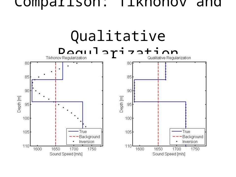
Comparison: Tikhonov and Qualitative Regularization

Approximate Equality Constraints

Relative Equality Constraint:

Find a solution that satisfies the data: Gm = d

Lm = 0

Am = αAbsolute Equality Constraint:

The solution is given by:2 2 11 2ˆ ( )T T T T m G G L L A A G d

The absolute equality constraint is chosen to restrict perturbations from the background profile near the sea surface and seafloor.

used to constrain the water column inverse problem

The matrix specifies where to apply the absolute equality constraint. The vector specifies the value the solution should take at these points.α

A

The relative equality constraint is the well known smoothness constraint of Tikhonov regularization.

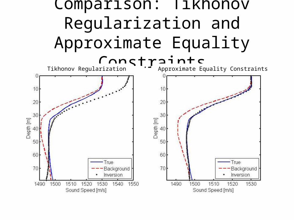
Comparison: Tikhonov Regularization and Approximate Equality Constraints

Approximate Equality ConstraintsTikhonov Regularization

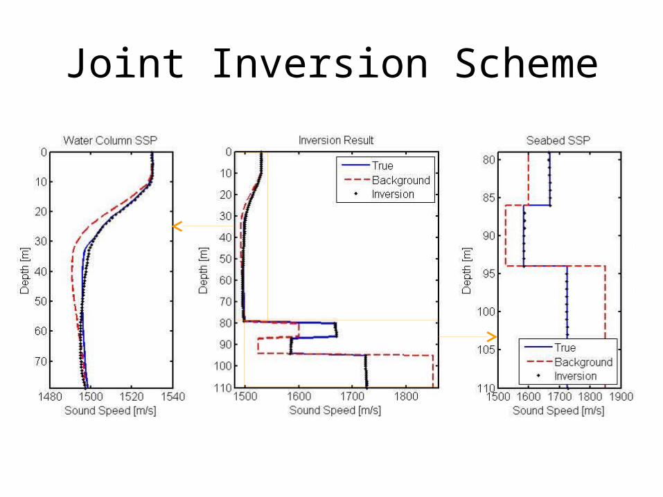
Joint Inversion Scheme

2 21 2

ˆ T T T -1 Tm = (G G + λ L L+ λ A A) (G d)2ˆq q

T T -1 Tm = (G G + λ L L ) G d

2 21 2

ˆq q

T T T -1 Tm = (G G + λ L L + λ A A) (G d)

Synthesis of qualitative regularization and approximate equality constraints to estimate water column and seabed sound speed profiles simultaneously.

Qualitative Regularization Approximate Equality Constraints

Synthesis of Qualitative Regularization and Approximate Equality Constraints

Used to resolve the discontinuity in the sound speed profile at the seafloor as well as discontinuities in the seabed

Used constrain the solution for the water column near the sea surface and seafloor where the data alone is insufficient to determine the solution

Robustness of the Algorithms• Effect of incorrect

assumptions about the water column when inverting for the sediment sound speed profile

• Effect of incorrect assumptions about the seabed when inverting for the water column sound speed profile

?

?

Separate Seabed InversionPoor knowledge of the water column sound speed profile causes errors in the solution for the seabed sound speed profile.

113 m/s

Separate Water Column InversionPoor knowledge of the seabed sound speed profile causes errors in the solution for the water column sound speed profile.

8 m/s

Rms error = 4.2 m/s

Joint WC and Seabed InversionPrimary benefit of the joint inversion scheme is that the solution does not suffer from erroneous assumptions about the other profile.

Model Resolution

1( )T Tm

R G GG G

2

1, 2

( )

( )

N

m ijji

m ii

L

RR

R

Model resolution matrix Resolution length

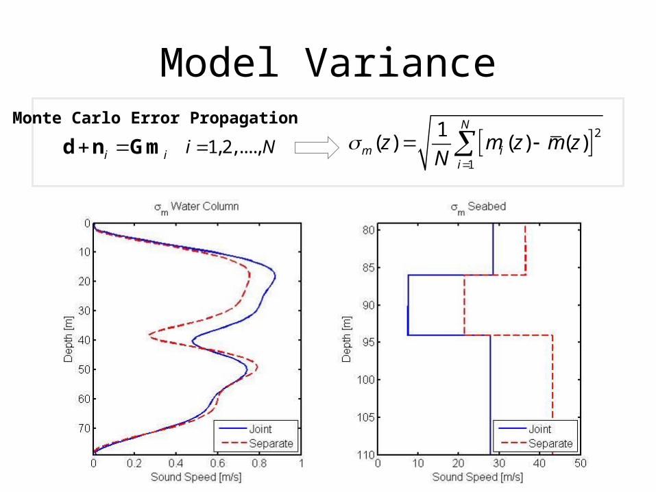
Model VarianceMonte Carlo Error Propagation

1,2,....,i Ni i d n Gm 21

1( ) ( ) ( )

N

m ii

z m z m zN

Summary• Simultaneous inversion of seabed and water column sound

speed profiles– Use of qualitative regularization to resolve the discontinuity in the

sound speed profile at the seafloor as well as additional discontinuities within the seabed

– Use of approximate equality constraints to constrain the solution where the data was inadequate to determine the solution

– Obtain accurate solutions for both seabed and water column sound speed profiles when neither profile is known

• Resolution and Variance– Separate inversion schemes provide a solution with higher resolution– Joint inversion scheme provides a solution with lower variance that is

more stable

Thank You

Questions?

Ill-Posed Problem

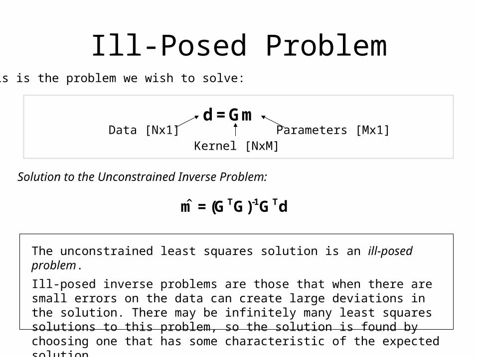
d = GmParameters [Mx1]Data [Nx1]

Kernel [NxM]

This is the problem we wish to solve:

Solution to the Unconstrained Inverse Problem:

ˆ T -1 Tm = (G G) G d

The unconstrained least squares solution is an ill-posed problem.

Ill-posed inverse problems are those that when there are small errors on the data can create large deviations in the solution. There may be infinitely many least squares solutions to this problem, so the solution is found by choosing one that has some characteristic of the expected solution.

Wave Number EstimationThe Hankel Transform Pair using the far field approximation

4

0 0( ; , ) ( ; , )2

r

iik r

r

r

eg k z z p r z z re dr

k

4

0 0( ; , ) ( ; , )2

r

iik r

r r r

ep r z z g k z z k e dk

r

1rk r

The Short-Time Fourier Transform (STFT)

Auto Regression (AR)

1

p

n k n kk

x a x

2

22

11

ARp i fkT

kk

TP

a e

4

0 0ˆ ˆ( ; , , ) ( ; ) ( ; , )2

r

iik r

r L

r

eg k r z z w r r p r z z re dr

k

Hankel Transform Estimate

Auto Regressive Spectrum

Separate Seabed InversionAn improved solution for the seabed sound speed profile can be obtained using the inverted water column sound speed profile.

19 m/s

Joint Inversion Scheme

Faulty a priori InformationFaulty a priori information will cause errors in the solution: incorrect values for the absolute constraints and layer depths will be reflected in the solutions.

Mismatch caused by incorrect values for the absolute constraint.

Mismatch caused by incorrect values for the layer depths.

Separate Water Column InversionThe solution for the water column sound speed profile can be improved by using a subset of low order wave number data.

3 m/s

Rms error = 0.7 m/s

Resolution and VarianceIt is essential to investigate how well the solution to the inverse problem represents the true model parameter values.

Model resolution and model variance are calculated for each of the water column and seabed inverse problems using both the separate and joint techniques.

• Model resolution is examined to characterize the bias of the generalized inverse.

• It shows how closely the solution matches the true model given exact data and assuming the known parameters are exact.

• Model variance is studied to understand the effect of data errors. • It is a measure how inaccuracies in the data affect the solution.

1( )T Tm

R G GG G

2

1, 2

( )

( )

N

m ijji

m ii

L

RR

R

Model resolution matrix

Resolution length

m R IFor perfect resolution:

, 1i i LR

For perfect resolution:

Rm is symmetric matrix that describes how the inverse smears out the true model.

Else:

Else:

, 1i i LR

Model Resolution

0 0

0

ˆ ( ) ( , ) ( )D

m z R z z m z dzThe continuous inverse problem is inherently underdetermined. All estimates of the model parameters must be given in terms of local averages.

Model Variance

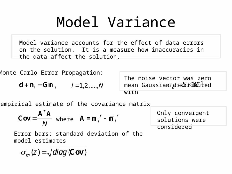
Monte Carlo Error Propagation:

T

NA A

Cov T Ti iA =m m

1,2,....,i N

where

The empirical estimate of the covariance matrix

i i d n Gm

( ) ( )m z diag Cov

Error bars: standard deviation of the model estimates

Model variance accounts for the effect of data errors on the solution. It is a measure how inaccuracies in the data affect the solution.

The noise vector was zero mean Gaussian distributed with 45 10d

Only convergent solutions were considered

1( )k

s

scond G

Solution Stability

where s1 and sk are the largest and smallest singular values of G.

A measure of the instability of the solution to an inverse problem is given by its condition number.

Separate Seabed Inversion

Separate Water Column Inversion

Joint Seabed and Water Column Inversion

8.86x109 2.49x102 1.90x102

The condition number can be interpreted as the rate at which the solution m will change with respect to a change in the data d. Thus, if the condition number is large, even a small error in d may cause a large error in m.