simultaneous estimation of system and input parameters from output measurements

74

Dow

nloa

ded

from

asc

elib

rary

.org

by

RO

BE

RT

SON

EN

GIN

EE

RIN

G &

on

09/1

1/13

. Cop

yrig

ht A

SCE

. For

per

sona

l use

onl

y; a

ll ri

ghts

res

erve

d.

SIMULTANEOUS ESTIMATION OF SYSTEM AND INPUT PARAMETERS

FROM OUTPUT MEASUREMENTS

By Tinghui Shi,1 Nicholas P. Jones,2 Member, ASCE, and J. Hugh Ellis,3 Member, ASCE

ABSTRACT: System identification of very large structures is of necessity accomplished by analyzing outputmeasurements, as in the case of ambient vibration surveys. Conventional techniques typically identify systemparameters by assuming (arguably) that the input is locally Gaussian white, and in so doing, effectively reducethe number of degrees of freedom of the estimation problem to a more tractable number. This paper describesa new approach that has several novel attributes, among them, elimination of the need for the Gaussian whiteinput assumption. The approach involves a filter applied to an identification problem formulated in the frequencydomain. The filter simultaneously estimates both system parameters and input excitation characteristics. Theestimates we obtain are not guaranteed to be unique (as is true in all other approaches: simultaneous estimationof both system and input possesses too many degrees of freedom to guarantee uniqueness); but we do, none-theless, identify system parameters and input excitation characteristics that are physically plausible and intuitivelyreasonable, without making input excitation assumptions. Simulated and laboratory experimental data are usedto verify the algorithm and demonstrate its advantages over conventional approaches.

INTRODUCTION

Full-scale measurement is typically the only assured methodfor verification of analysis and design procedures for largestructures (e.g., bridges and buildings). Short-term ambient vi-bration surveys (AVS) have been used primarily for the esti-mation of dynamic properties of such structures, but not forthe assessment and measurement of input characteristics. Ofparticular concern are the difficulties associated with the esti-mation of structural dynamic parameters such as damping ra-tio, which is a critical parameter in the estimation of structuralresponse to dynamic loads. The fact that the excitation forthese types of structures is typically unmeasurable, and thepresence of closely spaced modal peaks, serve to complicatethe estimation problem. Moreover, most existing techniquesdo not explicitly model the characteristics of excitation forcesand therefore make no attempt to estimate them. A commonapproach assumes that input excitations are locally Gaussianwhite (they are not)—an assumption that makes the estimationproblem more tractable by reducing the number of degrees offreedom of the associated estimation problem.

These types of unknown input identification problems haveattracted interest in recent years in a number of different con-texts (e.g., Beck et al. 1994; Conte and Krishnan 1995). Theability to reliably estimate dynamic system characteristics us-ing ambient environmental loading is attractive for such ap-plications as structural health monitoring and the determina-tion and verification of excitation models. Improvedprocedures are needed that can provide reliable estimates ofsystem parameters (including some assessment of confidencein those estimates) and then, by effectively turning the struc-tural system itself into a megatransducer, permit the estimationof input characteristics.

We develop in this paper an algorithm for system identifi-cation that simultaneously estimates system parameters and in-put power spectral density. The algorithm is essentially an ex-tended Kalman filter, but applied to a dynamic system model

1Former Grad. Student, Dept. of Civ. Engrg., Johns Hopkins Univ.,Baltimore, MD 21218-2686.

2Prof., Dept. of Civ. Engrg., Johns Hopkins Univ., Baltimore, MD.3Prof., Dept. of Geography and Envir. Engrg., and Dept. of Civ.

Engrg., Johns Hopkins Univ., Baltimore, MD.Note. Special Editor: Roger Ghanem. Discussion open until December

1, 2000. To extend the closing date one month, a written request mustbe filed with the ASCE Manager of Journals. The manuscript for thispaper was submitted for review and possible publication on February 25,2000. This paper is part of the Journal of Engineering Mechanics, Vol.126, No. 7, July, 2000. qASCE, ISSN 0733-9399/00/0007-0746–0753/$8.00 1 $.50 per page. Paper No. 22247.

6 / JOURNAL OF ENGINEERING MECHANICS / JULY 2000

J. Eng. Mech. 20

suitably formulated in the frequency domain. A critical attrib-ute of our approach is that it does not require an assumptionof input excitation form (e.g., Gaussian white). The paper be-gins with a brief statement of the generalized multi-degree-of-freedom vibration problem, including a mathematical charac-terization of noise-corrupted measurements. Estimation of theparameters of the system transfer function is then described.We follow with an overview of existing system identificationtechniques, leading first to a description of the filter algorithm,and then to its application to single-degree-of-freedom prob-lems formulated in the frequency domain. Numerical and lab-oratory simulations verify that the new approach reliably andefficiently identifies both system and input power spectral den-sity parameters.

GENERAL MDOF SYSTEM

The mathematical description of the general linear multi-degree-of-freedom (MDOF) vibrational problem is formulatedas

M y 1 C y 1 K y = L f (1)0 0 0 0

where M0 = mass matrix; C0 = damping matrix; K0 = stiffnessmatrix; L0 = excitation coefficient matrix; y = displacementvector; and f = random excitation force vector. The above-noted matrices and vectors have internally consistent dimen-sions, but we note that the dimension of y may be differentfrom that of z. Moreover, y and z can represent different quan-tities; for example, y might be displacement whereas z couldbe acceleration history.

At time tk = kDt, we assumed that n measurements are taken,i.e.

z(t ) = y(t ) 1 v (2)k k k

where z(tk) is an n-dimensional observation; and vk is an ob-servation noise vector, generally assumed to be Gaussianwhite, with covariance matrix Rk.

EXISTING IDENTIFICATION PROCEDURES

System identification methods are classified as parametricand nonparametric, and time domain and frequency domain(Bekey 1970; Astrom and Eykhoff 1971; Nieman et al. 1971;Bowles and Straeter 1972; Sage 1972; Eykhoff 1974; Kozinand Natke 1986; Ljung 1987). In state-space form, (1) and (2)can be written

x = Fx 1 Gf (3)

00.126:746-753.

Dow

nloa

ded

from

asc

elib

rary

.org

by

RO

BE

RT

SON

EN

GIN

EE

RIN

G &

on

09/1

1/13

. Cop

yrig

ht A

SCE

. For

per

sona

l use

onl

y; a

ll ri

ghts

res

erve

d.

z(t ) = Mx(t ) 1 v (4)k k k

where

y 0 I 0x = , F = , G = ,21 21 21S D S D S Dy 2M K 2M C M L0 0 0 0 0 0

0M = (I 0), f = S Df0

in which I is an n 3 n identity matrix; and 0 is an n 3 n zeromatrix.

Given knowledge of the input excitation, parametric, time-domain SID has certain advantages over other SID techniqueswhen applied to vibrational problems (Imai et al. 1989; Sarkar1992). Algorithms for parameter estimation using state-spaceequations generally fall into three categories: (1) the ordinaryleast squares (OLS) method; (2) the instrumental variable (IV)method; and (3) the maximum likelihood (ML) method. Thereare, in addition, several derivative methods that have been ap-plied to the structural vibration problem: the Ibrahim time do-main method (ITD) (Ibrahim 1977) and its modified form(MITD) (Sarkar 1992); the eigensystem realization algorithm(ERA) (Juang and Pappa 1984); and the random decrementmethod (Vandiver 1982). All of the above-mentioned methodsare not readily applicable to the unknown input case (Pandit1991).

Recent work has also seen the use of auto-regressive-mov-ing-average (ARMA) algorithms for identification problems(e.g., Pandit 1991). These methods portray the current systemoutput in terms of previous input and output, and current andpreceeding noise. They are widely used and are adaptable tomany forms. For random excitation problems, however, theequivalence of the covariance function between the discreteARMA model and the continuous physical model must be es-tablished to obtain satisfactory results, and identification ofthese relations is highly problematic.

KALMAN FILTER

Since 1960, the Kalman filter has been widely used to ob-tain estimates of state variables whose values are uncertain(Kalman 1960; Jazwinski 1970). The extended Kalman filterconsiders system parameters as part of an augmented state vec-tor. Inherent in the Kalman filter approach is the flexibility ofeasily incorporating system dynamics equations into the al-gorithm as well as the provision for uncertainty in the systemmodel.

Hoshiya and Saito (1984) and Maruyama et al. (1989) rep-resented system parameters as state variables and used an ex-tended Kalman filter applied to a frequency domain modelwith weighted global iteration to identify optimal parametervalues. This procedure is equivalent to using a weighted re-cursive least-squares (instead of regular least-squares) im-plementation of the filter (Maybeck 1982). Maruyama’s for-mulations involve earthquake engineering, where inputknowledge (in the form of base acceleration) is typically avail-able.

Hoshiya and Sutoh (1993) also demonstrate the applicationof a Kalman filter algorithm using weighted local iteration tothe problem of identification of unknown physical parametersin a static finite-element model. In this application, the filteris implemented in the spatial domain, with the results fromthe finite-element calculations at a number of locations usedin the observation vector. An implication of this work is thatif measured (rather than computed) data are used, the Kalmanfilter can be used to estimate the physical parameters of thereal system. A recent extension of this work (Hoshiya andYoshida 1995) was successfully applied to the problem ofidentifying the characteristics of a spatially distributed Gauss-ian random field.

J. Eng. Mech. 20

These examples point up the fact that although formulatedoriginally in the time domain, the Kalman filter has muchbroader applicability, e.g., in curve fitting when the form ofthe equation for the curve is considered to be potentially inerror (Strang 1986). There is nothing inherent in Kalman filtertheory or practice that restricts usage to the time domain. It issimply a data processing algorithm that—provided basic as-sumptions are satisfied (or approximately satisfied)—willelicit desired model information from the raw data. As will beshown below, in our frequency-domain application, a time-stepin the original formulation is replaced by a ‘‘frequency step’’and serves as the process evolution index. When the filter isapplied to a problem formulated in the frequency domain, theinput auto- and cross-spectral density functions (in parameter-ized form or as discrete ordinates) can be viewed as state var-iables and the observation can be a function of the auto- andcross-spectral densities of output measurements. In the appli-cations described herein, the augmented state vector consistsof either the parameters of an assumed form of the input PSDplus natural frequency and damping parameters, or, alterna-tively, input spectrum ordinates, augmented by the dynamicsystem parameters (frequency and damping ratio).

The method has been tested with numerical simulations andcontrolled laboratory experimental data for an SDOF system,and will be ultimately applied to the analysis of accelerationdata recorded on a number of full-scale structures. The con-trolled experiments enable assessment of the new technique tobe made by comparison with more conventional approaches.

MODEL DEVELOPMENT

Kalman Filter Algorithm

Kalman filter techniques use linear, recursive, least-squareestimation methods designed to minimize the error covarianceof state variables while incorporating both process and mea-surement uncertainties (Gelb 1974). The filter is an optimalestimator in the sense that it minimizes the mean-square esti-mation errors of state variables (Gelb 1974). An added benefitof this type of filtering is that the variances associated withstate estimates are simultaneously obtained. The filter pre-sented below is continuous-discrete: continuous in the sensethat the physical model is continuous, discrete in that obser-vations are made at discrete intervals.

A brief overview of the Kalman filtering process applied inthe time domain (Jazwinski 1970; Maybeck 1982; Koh andSee 1994) is presented below, followed by the adaptation to aproblem formulated in the frequency domain.

Consider the general dynamic system described by

dx(t)= f [x(t), t] 1 Gw(t) w(t) ; N[0, Q(t)] (5)

dt

with observations at tk = kDt, k = 1, 2, . . .. The observationvector z(k) is defined

z(k) = h[x(k), k] 1 v (6)k

in which x(t), x(k) = state vector; w(t) = system noise withcovariance matrix Q; vk = observation noise vector with co-variance matrix Rk; f [x(t), t] = system dynamics function; andh[x(k), k] is an observation function. It is hereafter denotedthat x(k) = x(tk), z(k) = z(tk), etc., for simplicity.

Now consider the reference state x, which satisfies

dx= f [x(t), t] (7)

dt

The deviation between the actual state and reference state attk = kDt can be written (Jazwinski 1970) as

JOURNAL OF ENGINEERING MECHANICS / JULY 2000 / 747

00.126:746-753.

Dow

nloa

ded

from

asc

elib

rary

.org

by

RO

BE

RT

SON

EN

GIN

EE

RIN

G &

on

09/1

1/13

. Cop

yrig

ht A

SCE

. For

per

sona

l use

onl

y; a

ll ri

ghts

res

erve

d.

dx(k) = x(k) 2 x(k) (8)

Similarly,

dz(k) = z(k) 2 z(k) (9)

where

z(k) = h(x(k), k) (10)

The linearized system dynamic matrix can be written

f(x(t), t)F(t, x) = (11)Tx

The deviation forms of (8) and (9) are thus

dx(k 1 1) = F[k 1 1, k; x(k uk)]dx(k) 1 w(k 1 1) (12)

dz(k) = M[k; x(k)]dx(k) 1 v (13)k

where

h[x(k), k]M[k; x(k)] = (14)Tx (k)

is an observation matrix, and

F[k 1 1, k; x(k uk)] ' I 1 DtF(k, x) (15)

is a state transition matrix, in which i u j represents the esti-mation of step i from the observation knowledge up to step j,and I = identity matrix. At time tk = kDt, given the estimateof state variable x(k uk) and error covariance matrix P(k uk), theextended Kalman filter consists of the following equations.

Prediction:(k11)Dt

x(k 1 1 uk) = x(k uk) 1 f [x(t), t] dt (16)EkDt

T TP(k 1 1 uk) = FP(k uk)F 1 GQ G (17)d

Kalman Gain:T T 21K = P(k 1 1 uk)M {MP(k 1 1 uk)M 1 R} (18)

Update:

x(k 1 1 uk 1 1) = x(k 1 1 uk) 1 K{z 2 h} (19)

T TP(k 1 1 uk 1 1) = {I 2 KM}P(k 1 1 uk){I 2 KM} 1 KRK (20)

where F = F[k 1 1, k; x(k uk)]; Qd = Qd(k 1 1) = (k11)Dt*kDt

Q(t) dt; K = K[k 1 1; x(k 1 1 uk)]; M = M[k 1 1; x(k 11 uk)]; R = Rk11; z = z(k 1 1); and h = h[x(k 1 1 uk), k 1 1].

The error covariance updating step of (20) follows the Jo-seph form (Maybeck 1982), the advantage of which is that itguarantees P(k 1 1 uk 1 1) to be symmetric and positive semi-definite, and therefore yields improved (i.e., more stable) nu-merical performance.

Identification of SDOF System in Frequency Domain

When Kalman filtering is applied to a frequency-domaindescription of the SDOF system, system parameters and theinput power spectral density are used in the augmented statevector. With suitable frequency-domain interpretations of theconstitutive functions g and G, the system and observationequations [(5) and (6)] can be written as

System Model:

ds(v)= g(s, v) 1 Gw(v) w(v) ; N(0, Q(v)) (21)

dv

Alternatively, the output power spectral density could be usedin the algorithm and the input PSD estimate obtained after


J. Eng. Mech. 200

running the filter. It is more efficient, however, to use the inputspectral density function. The frequency-domain-formulatedfilter comprises the following components:

Measurement/Observation Model:

z(k) = h(s(k), k) 1 v ; k = 1, 2, . . . ; v(k) ; N(0, R ) (22)k k

The observation matrix M(k, s) and system dynamic matrixF(v, s) are defined as

h(s(k), k)M(k; s(k)) = (23)Ts (k)

g(s(v), v)F(v, s) = (24)Ts

and the state transition matrix can be approximated by

F[k 1 1, k; s(k uk)] ' I 1 Dv[F] (25)s(kuk)

where the augmented state vector s(v) or s(k) is now taken asa function in the frequency domain. The terms w(v) and vk

now represent frequency domain noise terms and are assumedto be Gaussian white.

For the identification algorithm used here, there are two al-ternative state vector representations. If the input spectral den-sity matrix is known to be of a specific form described byparameters, a1, a2, . . . , then the state vector may be writtenas

Ts = {v , z, a , a , . . .} (26)n 1 2

In this case, natural frequency, damping ratio, and parametersa1, a2, . . . are constant and independent of frequency. There-fore, the derivative of these quantities with respect to fre-quency is zero. Nonetheless, it is appropriate to include modeluncertainty related to these parameters in order to reflect thepotential error inherent in modeling the actual vibrational sys-tem as an SDOF system (i.e., errors in frequency and dampingparameters) and to reflect the approximation associated withformulating the input PSD as a function of parameters a1,a2, . . ..

If the form of the input spectrum is known, its derivativecan be incorporated directly into g(s, v). This represents ad-ditional knowledge and can potentially improve the perfor-mance of the algorithm. Experience in a number of examplessuggests that this effort is not generally necessary, because ofthe satisfactory performance of the algorithm simply using g[ 0.

For the more general case in which the form of the inputpower spectral density is not known, the augmented state vec-tor s(v) is taken as

Ts(v) = {S (v), v , z} (27)f n

where Sf(v) = input PSD, a function of frequency v. Analo-gous to the time-domain implementation, Sf is identified ateach step as the natural frequency and damping estimates areupdated. In this formulation, the system dynamics describingthe evaluation of this state variable can still be written:

dS (v)f = 0 1 w (v) (28)sdv

where ws(v) is process noise, assumed herein to be Gaussianin the frequency domain. In this formulation, the filter modelsthe input power spectrum as constant with frequency, withuncertainty introduced through suitable assignment of ws(v).

The dynamic system (21) can therefore be taken as

ds= w(v) w(v) ; N[0, Q(v)] (29)

dv

0.126:746-753.

Dow

nloa

ded

from

asc

elib

rary

.org

by

RO

BE

RT

SON

EN

GIN

EE

RIN

G &

on

09/1

1/13

. Cop

yrig

ht A

SCE

. For

per

sona

l use

onl

y; a

ll ri

ghts

res

erve

d.

This equation is not simply a steady-state equation, becausethe model uncertainty (or process noise) matrix Q is, in gen-eral, nonzero. If the quantity to be estimated, Sf(v), changeswith frequency (which it usually does), a different value isestimated at every step when measurement is included in thealgorithm. The matrix Q admits this change, and the optimalfiltering problem is a dynamic problem that cannot be for-mulated using recursive least-squares.

The matrix F in (24) reduces to an N 3 N zero matrix,where N is the number of state variables. The discrete statetransition matrix F in (25) is therefore

F(v, s) = I (30)

The prediction, gain, and updating equations of the filter inthis case become

Prediction:

s(k 1 1 uk) = s(k uk) (31)

P(k 1 1 uk) = P(k uk) 1 Q (32)d

Gain:

T T 21K = P(k 1 1 uk)M {MP(k 1 1 uk)M 1 R} (33)

Update:

s(k 1 1 uk 1 1) = s(k 1 1 uk) 1 K{z 2 h} (34)

T TP(k 1 1 uk 1 1) = {I 2 KM}P(k 1 1 uk){I 2 KM} 1 KRK (35)

where Qd = Qd(k 1 1) = Q(v) dv; K = K[k 1 1; s(k(k11)Dv*kDv

1 1 uk)]; M = M[k 1 1; s(k 1 1 uk)]; R = Rk11; z = z(k 1 1);and h = h[s(k 1 1 uk), k 1 1].

The following relation can be used to directly use acceler-ation data (Bendat et al. 1986):

4 4 2S (v) = v S (v) = v uH(v) u S (v) (36)¨ z fz

where Sz(v) and = PSD of the displacement and theS (v)z

acceleration, respectively, and H(v) is the transfer functionbetween the forcing function f and the displacement responsez. The observed spectral density functions vary rapidly aroundthe natural frequency so the filter tends to diverge if the ele-ments in are used directly as the observation vector. ThisS (v)z

difficulty may be overcome by using a natural logarithmicform of the PSD, and hence the generalized observation func-tion h in (22) is reduced to a scalar:

h(v) = ln(S (v)) (37)z

and (22) becomes

z (k) = h(k) 1 v (38)g k

Thereafter, the observation matrix M can be obtained through(23):

hM = (39)Ts

It is noted that by using the logarithmic transformation in(37), an artificial nonlinear observation function is introduced,rendering the algorithm less sensitive than that based on (36).After transformation, observation error is also no longerGaussian, but this we view as nonproblematic [e.g., ‘‘. . . ifthe Gaussian noise assumption is removed, the Kalman filtercan be shown to be the best (minimum error variance) filterout of the class of linear unbiased filters’’ (Maybeck 1979,page 7)].

After the state transition matrix (30) and observation matrix(39) have been defined, standard procedures [(31)–(35)] candirectly be used to obtain state and error covariance estimates.

J. Eng. Mech. 20

FIG. 1. Acceleration PSD of Computer-Simulated Output Data

The frequency domain formulation presents several advan-tages over its time-domain-based counterpart:

1. Only those parameters to be identified need to be rep-resented as state variables. It is not necessary, for ex-ample, to represent displacements and velocities as statevariables.

2. The system transition matrix is an identity matrix, com-pared to the nonlinear transition matrix (which has to belinearized) as required in the time-domain formulation.

3. Acceleration data can be used directly and the associatedintegration problems are avoided.

4. Sampling lag in the time domain corresponds to a knownphase lag in the frequency domain; therefore, compli-cations associated with nonsimultaneous sampling can betractably addressed.

EXAMPLES

Several examples will now be presented to demonstrate theapplication of the above-described method. The exampleshighlight a number of features of the proposed method andinclude the use of both numerically simulated and experi-mental data.

The equations of motion of an SDOF vibrational system canbe written

2x 1 2zv x 1 v x = f /m (40)n n

where vn = is the circular natural frequency; and z =k/mÏc/2mvn is the damping ratio.

Numerical Simulation: Markov Process Excitation

A first-order Markov stochastic process with a PSD function1/(1 1 0.05v2) was simulated using the spectral representationmethod (Shinozuka 1991), with simulation cut-off frequencyvu = 3.0 rad/s, Dt = 0.02 s, M = 65,536 points, giving Dv =0.00479 rad/s. A zero-mean, uncorrelated, 20% noise-to-signal(sn/ss) ratio random white noise was added to the simulatedrandom process. The response displacement, velocity, and ac-celeration of an SDOF system with natural frequency 2.0 rad/sand damping ratio 5%, were calculated using an implicit trape-zoidal rule integration scheme. The PSD of the numerical out-put is shown in Fig. 1.

Two approaches were used in this example. The first ap-proach presumed that the random excitation PSD was of theform a1/(1 1 a2v

2). The filter was implemented to identify thefrequency, damping ratio, and parameters a1, a2. The step sizefor the filter was taken as Dv = 0.00479 rad/s; the startingfrequency v = 1 rad/s (frequency point k = 208), ending fre-


00.126:746-753.

Dow

nloa

ded

from

asc

elib

rary

.org

by

RO

BE

RT

SON

EN

GIN

EE

RIN

G &

on

09/1

1/13

. Cop

yrig

ht A

SCE

. For

per

sona

l use

onl

y; a

ll ri

ghts

res

erve

d.

TABLE 1. SDOF Numerical Data—Parameter Identification

Kalman filter(1)

Frequency(rad/s)

(2)Damping

(3)a1

(4)a2

(5)

Initial value(standard deviation)

1.50(0.316)

0.1(0.01)

2.0(0.316)

0.1(0.1)

1st iteration 2.0001 0.0676 1.2294 0.07262nd iteration 2.0020 0.0547 1.0543 0.05613rd iteration 2.0005 0.0514 1.0299 0.05264th iteration 2.0002 0.0504 1.0124 0.05175th iteration

(standard deviation)2.0002

(0.0095)0.0504

(0.0045)1.0104

(0.0776)0.0517

(0.0093)Theoretical 2.0 0.05 1.0 0.05

quency v = 6 rad/s (frequency point k = 1,251); the modeluncertainty matrix Qd was assumed to be zero (since the nu-merical model can be considered to be ‘‘perfect’’ in this im-plementation); and the observation uncertainty was arbitrarilyset as R = I. Five iterations (over the frequency axis) wereperformed, with the final conditions of one iteration used asinitial conditions for the next.

The initial estimates and standard deviations of the statevariables and the results of the identification are shown inTable 1. Figs. 2(a–d) show the evolution of identified param-eters and their standard deviates in the last iteration. Note thatthis example is equivalent to a recursive least-squares esti-mation, since the model uncertainty was set to be zero.

This same simulation problem was also identified by defin-ing the input PSD Sf(v) itself as a state variable. A similarprocedure was used, except that in this case the error covari-ance matrix Qd was assumed to be nonzero, since the actual


J. Eng. Mech. 2

TABLE 2. SDOF Numerical Data—Input PSD Identification

Kalman filter(1)

Frequency(rad/s)

(2)Damping

(3)


1.50(0.316)

0.1(0.01)

First iteration 2.0039 0.0535Second iteration 1.9998 0.0506Third iteration 2.0001 0.0504Fourth iteration 2.0001 0.0504Fifth iteration

(standard deviation)2.0000

(0.033)0.0503

(0.0087)Theoretical 2.0 0.05

input PSD is a single realization of the random process andtherefore differs from its functional description. The initial es-timate of the input PSD was 1.0; its error covariance P0 = 0.1;and model uncertainty Qd = 0.1. Five iterations were per-formed and the results of the procedure are shown in Table 2.The simulated and identified input PSD are shown in Fig. 3.Five iterations are sufficient to determine system characteris-tics and to satisfactorily estimate the input PSD.

Numerical Simulation: Kanai-Tajimi EarthquakeSpectrum

It is expected that in the case of close-to-white input PSD,an extended-Kalman-filter-based method will give results thatare at least as good as those from the recursive-least-squaresmethod. However, in the case of a strongly nonwhite inputPSD, the filter approach, which takes model uncertainty into

FIG. 2. Computer-Simulated Case I: (a) Natural Frequency Estimation; (b) Damping Ratio Estimation; (c) Input PSD Parameter (a1)Estimation; (d) Input PSD Parameter (a2) Estimation (Dashed Lines Are One Sigma Bounds)

000.126:746-753.

Dow

nloa

ded

from

asc

elib

rary

.org

by

RO

BE

RT

SON

EN

GIN

EE

RIN

G &

on

09/1

1/13

. Cop

yrig

ht A

SCE

. For

per

sona

l use

onl

y; a

ll ri

ghts

res

erve

d.

FIG. 3. Simulated and Identified Input PSD (Solid Line Is The-oretical, Dashed Line Is Identified)

account, is expected to give better results than the recursive-least-squares method, which considers only measurement un-certainty. An additional numerical example of an SDOF sys-tem under a Kanai-Tajimi model for earthquake excitation wasstudied to demonstrate the advantages of the filter over therecursive-least-squares method.

A Kanai-Tajimi random process model of the form

4 2 2 2f (v 1 4v v z )0 g g gS (v) = (41)z 2 2 2 2 2 2(v 2 v ) 1 4v v zg g g

was assumed for the ground acceleration.An SDOF system with vs = 12.0 rad/s and zs = 0.05 was

simulated under input parameters f0 = 1.0, vg = 15.7 rad/s,and zg = 0.60. The simulation was performed under cut-offfrequency vc = 40.0 rad/s, 262,144 time points with intervalDt = 0.005 s, and 8,344 frequency points with interval Dw =0.00479 rad/s. The system was then identified under two con-ditions:

1. Noise-free2. Noise-contaminated with 10% noise-to-signal ratio

The covariance of observation noise R was arbitrarily set at1.0; the covariances of the system noise associated with thenatural frequency and damping ratio were set at relativelysmall values to represent these system characteristics essen-tially as constant in the frequency domain. The covariance of

J. Eng. Mech. 20

FIG. 4. SDOF Experimental Schematic

system noise associated with the input PSD was varied tostudy the effect of model uncertainty on the accuracy of theestimation. The results are listed in Table 3.

The recursive-least-squares method (Q = 0) does not giveaccurate results, especially in the estimation of the input PSD.RLS estimation cannot capture the frequency dependence ofthe input spectrum in this example (by forcing it to be con-stant), with resulting undesirable consequences for the qualityof the estimates of the other parameters. This demonstrates akey advantage of the proposed method. In practice, input spec-tra are not white. The filter enables quantitative incorporationof this fact, thereby improving the quality of the estimates ofall system and input parameters.

Through trial and error, the most accurate results were ob-tained using Qinput = 1023 2 1024 for the noise-free case andQinput = 1024 2 1025 for the noise-contaminated case. The in-crease in the optimal Q value from the noise-free case to thenoise-contaminated case indicates that the filter ‘‘trusts’’ morein the model than the observation because of the presence ofnoise in the measurement.

Laboratory Simulation

A miniature one-story building model with flexible alumi-num walls and a rigid aluminum floor was constructed (Fig.4) with the base rigidly fixed to a horizontal shake table. Thegoverning equation of motion of this structure under base ex-citation is

mx 1 c(x 2 y) 1 k(x 2 y) = 0 (42)

TABLE 3. Parametric Study of Model Uncertainty

Cases(1)

Qv

(2)Qz

(3)Qin

(4)v(5)

v9(6)

Error %(7)

z(8)

z9(9)

Error %(10)

Input error %(11)

1 0.01027

1027

0.01028

1028

0.00.0

1027

12.012.012.0

11.952011.881411.9145

0.400.990.71

0.050.050.05

0.02560.02280.0233

48.7454.4553.35

60.4360.2451.46

1027

1027

1027

1028

1028

1028

1026

1025

1024

12.012.012.0

11.948711.984011.9865

0.430.1330.11

0.050.050.05

0.03430.04380.0480

33.1412.39

4.00

29.7012.02

4.241027

1027

1027

1028

1028

1028

1023

1022

1021

12.012.012.0

11.976511.933211.6308

0.200.563.08

0.050.050.05

0.04910.04910.0338

1.781.90

32.40

1.992.70

12.222 0.0

1027

1027

0.01028

1028

0.00.0

1027

12.012.012.0

11.882111.835411.8700

0.981.371.08

0.050.050.05

0.02760.02450.0248

44.9151.0750.36

60.6260.3353.63

1027

1027

1027

1028

1028

1028

1026

1025

1024

12.012.012.0

11.902211.932911.9198

0.810.560.67

0.050.050.05

0.03660.04650.0496

26.816.900.75

32.7315.5210.06

1027

1027

1027

1028

1028

1028

1023

1022

1021

12.012.012.0

11.450810.542710.2584

4.5812.1414.51

0.050.050.05

0.00970.00000.0000

80.61100.00100.00

198.55193.51

70.19


00.126:746-753.

Dow

nloa

ded

from

asc

elib

rary

.org

by

RO

BE

RT

SON

EN

GIN

EE

RIN

G &

on

09/1

1/13

. Cop

yrig

ht A

SCE

. For

per

sona

l use

onl

y; a

ll ri

ghts

res

erve

d.

TABLE 4. Identification of Laboratory-Simulated Data

Kalman filter(1)

Frequency(rad/s)

(2)Damping

(3)


40.0(2.00)

0.1000(0.032)

Model uncertainty Q 1027 10210

First iteration 53.22 0.02035Second iteration 54.00 0.02593Third iteration 53.99 0.02616Fourth iteration 53.98 0.02635Fifth iteration

(standard deviation)53.98(0.25)

0.02633(0.0046)

Spectrum analyzer 55.21 0.0254I-DEAS test 53.86 0.0272

FIG. 6. Acceleration PSD of Base Excitation

FIG. 5. Acceleration PSD—Laboratory Simulated Output Data

where x = absolute motion of the first floor; and y = absolutemotion of the base. This equation can be rearranged as

2 2x 1 2zv x 1 v x = 2zv y 1 v y (43)n n n n

Two accelerometers were attached: one to the base and oneto the first floor. Data were recorded on a personal computerusing a 12-bit A/D converter. The signals were sampled at afrequency of 100 Hz. A 300-s experiment was conducted torecord the time history of both the base and first floor, with atotal of 30,720 data points recorded. The PSD was calculatedwith a Hanning window, 50% overlap of data points, resultingin 6 averages at a spectral resolution of 4,097/Nyquist interval.The PSD of the experimental output is shown in Fig. 5. ThePSD of base excitation is shown in Fig. 6.


J. Eng. Mech. 20

FIG. 7. (a) Acceleration PSDs (Solid Line Is Identified from4,087 Points, Dashed Line Is Recorded 513 Points); Laboratory-Simulated Output Data: (b) Natural Frequency Estimation; (c)Damping Ratio Estimation (Dashed Lines Are One SigmaBounds)

The PSD of the output acceleration data in this base-accel-eration case can be written as

2 2 2 2 4S (v) = uH(v) u (4z v v 1 v )S (v) (44)¨ ¨n nx y

H(v) = transfer function between the forcing function y (ab-solute displacement of the base) and the absolute response xof the first floor. Identification can be performed as in thenumerical example, except that in this case, Sf(v) = 2 2 2(4z v vn

1 After natural frequency, damping ratio, and Sf(v)4v )S (v).¨n y

are identified, the PSD of the base acceleration can be re-trieved.

The parameters and procedures were as follows:

00.126:746-753.

Dow

nloa

ded

from

asc

elib

rary

.org

by

RO

BE

RT

SON

EN

GIN

EE

RIN

G &

on

09/1

1/13

. Cop

yrig

ht A

SCE

. For

per

sona

l use

onl

y; a

ll ri

ghts

res

erve

d.

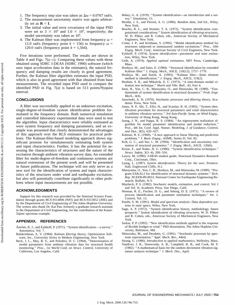
1. The frequency step size was taken as Dv = 0.0767 rad/s.2. The measurement uncertainty matrix was again arbitrar-

ily set as R = I.3. The initial value and error covariance of the input PSD

were set to 3 3 104 and 1.0 3 108, respectively; themodel uncertainty was taken as 106.

4. The Kalman filter was implemented from frequency v =12.0 rad/s (frequency point k = 156) to frequency v =120.0 rad/s (frequency point k = 1,564).

Five iterations were performed. The results are shown inTable 4 and Figs. 7(a–c). Comparing these values with thoseobtained using SDRC I-DEAS (SDRC 1990) software (whichuses input acceleration data in the estimates), the natural fre-quency and damping results are clearly in good agreement.Further, the Kalman filter algorithm estimates the input PSD,which is also in good agreement with that obtained from basemeasurements. The recorded input PSD used to compare theidentified PSD in Fig. 7(a) is based on 513 points/Nyquistinterval.

CONCLUSIONS

A filter was successfully applied to an unknown excitation,single-degree-of-freedom system identification problem for-mulated in the frequency domain. Both numerical simulationand controlled laboratory experimental data were used to testthe algorithm. Input characteristics were reliably estimated aswere system frequency and damping parameters, and an ex-ample was presented that clearly demonstrated the advantagesof this approach over the RLS estimator for practical prob-lems. The Kalman-filter-based modeling approach shows sig-nificant promise for simultaneously estimating both systemand input characteristics. Further, it has the potential for as-sessing the characteristics of structures and the nature of theexcitation through ambient vibration survey data. An extendedfilter for multi-degree-of-freedom and continuous systems arenatural extensions of the present work and will be presentedin future publications. The technique will not only serve as anew tool for the identification of system and input character-istics of the structures under wind and earthquake excitation,but also will potentially contribute significantly to other prob-lems where input measurements are not possible.

ACKNOWLEDGMENTS

Support for this research was provided by the National Science Foun-dation through grants BCS-9114006 (NPJ) and BCS-9313052 (JHE) andby the Department of Civil Engineering of The Johns Hopkins University.The writers also thank Dr. Kai Pan, formerly a graduate research assistantin the Department of Civil Engineering, for the contribution of the Kanai-Tajimi spectrum example.

APPENDIX. REFERENCES

Astrom, K. J., and Eykhoff, P. (1971). ‘‘System identification—a survey.’’Automatica, Vol. 7.

Balakrishnan, A. V. (1984). Kalman filtering theory, Optimization Soft-ware, Inc., University Series in Modern Engineering, New York.

Beck, J. L., May, B. S., and Polodori, D. C. (1994). ‘‘Determination ofmodal parameters from ambient vibration data for structural healthmonitoring.’’ Proc., 1st World Conf. on Struct. Control, University ofCalifornia, Los Angeles, Calif.

J. Eng. Mech. 200

Bekey, G. A. (1970). ‘‘System identification—an introduction and a sur-vey.’’ Simulation, 15.

Bendat, J. S., and Piersol, A. G. (1986). Random data, 2nd Ed., Wiley,New York.

Bowles, R. L., and Straeter, T. A. (1972). ‘‘System identification com-putational considerations.’’ System identification of vibrating structures,W. D. Pilkey and R. Cohen, eds., American Society of MechanicalEngineers, New York.

Conte, J. P., and Krishnan, S. (1995). ‘‘Modal identification method forstructures subjected to unmeasured random excitations.’’ Proc., 10thEngrg. Mech. Conf., American Society of Civil Engineers, New York.

Eykhoff, P. (1974). System identification—parameter and state estima-tion, Wiley, New York.

Gelb, A. (1974). Applied optimal estimation, MIT Press, Cambridge,Mass.

Hoshiya, M., and Saito, E. (1984). ‘‘Structural identification by extendedKalman filter.’’ J. Engrg. Mech., ASCE, 110(12), 1757–1770.

Hoshiya, M., and Sutoh, A. (1993). ‘‘Kalman filter—finite elementmethod in identification.’’ J. Engrg. Mech., ASCE, 119(2).

Ibrahim, S. R., and Mikulcik, E. C. (1973). ‘‘A time-domain modal vi-bration test technique.’’ Shock and Vibr. Bull., 43, Part 4.

Imai, H., Yun, C. B., Maruyama, O., and Shinozuka, M. (1989). ‘‘Fun-damentals of system identification in structural dynamics.’’ Prob. Engr.Mech., 4(4).

Jazwinski, A. H. (1970). Stochastic processes and filtering theory, Aca-demic Press, New York.

Jones, N. P., Shi, T., Ellis, H., and Scanlan, R. H. (1993). ‘‘System iden-tification procedure for structural parameters and wind characteristicsin ambient vibration surveys.’’ 3rd Asia-Pacific Symp. on Wind Engrg.,University of Hong Kong, Hong Kong.

Juang, J. N., and Pappa, R. S. (1984). ‘‘An eigensystem realization al-gorithm for modal parameter identification and modal reduction.’’Proc., 4th Int. Conf. Appl. Numer. Modeling, J. of Guidance, Control,and Dyn., 8(5), 620–627.

Kalman, R. E. (1960). ‘‘A new approach to linear filtering and predictionproblems.’’ J. Basic Engrg., ASME, Series D, Vol. 82.

Koh, G. C., and See, L. M. (1994). ‘‘Identification and uncertainty esti-mation of structural parameters.’’ J. Engrg. Mech., ASCE, 120(6).

Kozin, F., and Natke, H. G. (1986). ‘‘System identification techniques.’’Struct. Safety, 3(3–4), 269–316.

Lawry, M. (1990). I-DEAS student guide, Structural Dynamics ResearchCorp., Cincinnati, Ohio.

Ljung, L. (1987). System identification: Theory for the user, Prentice-Hall, Englewood Cliffs, N.J.

Maruyama, O., Yun, C. B., Hoshiya, M., and Shinozuka, M. (1989). ‘‘Pro-gram EXKAL2 for identification of structural dynamic systems.’’ Tech.Rep. NCEER-89-0014, National Center for Earthquake Engineering Re-search, Buffalo, N.Y.

Maybeck, P. S. (1982). Stochastic models, estimation, and control, Vol. Iand Vol. II, Academic Press, San Diego, Calif.

Nieman, R. E., Fischer, D. G., and Seborg, D. E. (1971). ‘‘A review ofprocess identification and parameter estimation techniques.’’ Int. J.Control, Vol. 13.

Pandit, S. M. (1991). Modal and spectrum analysis: Data dependent sys-tems in state space, Wiley, New York.

Sage, A. P. (1972). ‘‘System identification history, methodology, futureprospects.’’ System identification of vibrating structures, W. D. Pilkeyand R. Cohen, eds., American Society of Mechanical Engineers, NewYork.

Sarkar, P. P. (1992). ‘‘New identification methods applied to the responseof flexible bridges to wind.’’ PhD dissertation, The Johns Hopkins Uni-versity, Baltimore, Md.

Shinozuka, M., and Deodatis, G. (1991). ‘‘Stochastic processes by spec-trum representation.’’ Appl. Mech. Rev., 44(4).

Strang, G. (1986). Introduction to applied mathematics, Wellesley, Mass.Vandiver, J. K., Dunwoody, A. B., Campbell, R. B., and Cook, M. F.

(1982). ‘‘A mathematical basis for the random decrement vibration sig-nature analysis technique.’’ J. Mech. Des., April.


0.126:746-753.

simultaneous estimation of system and input parameters from output measurements

Documents