simulations of the primary cement placement in annular

Louisiana State UniversityLSU Digital Commons

LSU Master's Theses Graduate School

2012

Simulations of the primary cement placement inannular geometries during well completion usingcomputational fluid dynamics (CFD)Muhammad ZulqarnainLouisiana State University and Agricultural and Mechanical College, [email protected]

Follow this and additional works at: https://digitalcommons.lsu.edu/gradschool_theses

Part of the Petroleum Engineering Commons

This Thesis is brought to you for free and open access by the Graduate School at LSU Digital Commons. It has been accepted for inclusion in LSUMaster's Theses by an authorized graduate school editor of LSU Digital Commons. For more information, please contact [email protected].

Recommended CitationZulqarnain, Muhammad, "Simulations of the primary cement placement in annular geometries during well completion usingcomputational fluid dynamics (CFD)" (2012). LSU Master's Theses. 2022.https://digitalcommons.lsu.edu/gradschool_theses/2022

https://digitalcommons.lsu.edu?utm_source=digitalcommons.lsu.edu%2Fgradschool_theses%2F2022&utm_medium=PDF&utm_campaign=PDFCoverPages

https://digitalcommons.lsu.edu/gradschool_theses?utm_source=digitalcommons.lsu.edu%2Fgradschool_theses%2F2022&utm_medium=PDF&utm_campaign=PDFCoverPages

https://digitalcommons.lsu.edu/gradschool?utm_source=digitalcommons.lsu.edu%2Fgradschool_theses%2F2022&utm_medium=PDF&utm_campaign=PDFCoverPages

https://digitalcommons.lsu.edu/gradschool_theses?utm_source=digitalcommons.lsu.edu%2Fgradschool_theses%2F2022&utm_medium=PDF&utm_campaign=PDFCoverPages

http://network.bepress.com/hgg/discipline/245?utm_source=digitalcommons.lsu.edu%2Fgradschool_theses%2F2022&utm_medium=PDF&utm_campaign=PDFCoverPages

https://digitalcommons.lsu.edu/gradschool_theses/2022?utm_source=digitalcommons.lsu.edu%2Fgradschool_theses%2F2022&utm_medium=PDF&utm_campaign=PDFCoverPages

mailto:[email protected]

SIMULATIONS OF THE PRIMARY CEMENT PLACEMENT IN

ANNULAR GEOMETRIES DURING WELL COMPLETION USING

COMPUTATIONAL FLUID DYNAMICS (CFD)

A Thesis

Submitted to the Graduate Faculty of the

Louisiana State University and

Agricultural and Mechanical College

in partial fulfillment of the

requirements for the degree of

Master of Science in Petroleum Engineering.

in

The Craft and Hawkins Department of Petroleum Engineering

By

Muhammad Zulqarnain

M.Sc., Pakistan Institute of Engineering and Applied Sciences, Pakistan, 2003

May, 2012

ii

ACKNOWLEDGEMENTS

I am deeply thankful to my advisor, Dr. Mayank Tyagi for his support, guidance and

encouragement throughout the course of this work. His valuable inputs were extremely helpful

during this research work and thesis writing. He showed me many ways to approach a problem

and the need to be persistent in order to accomplish the tasks.

Thanks to Prof. A. K. Wojtanowicz and Prof. J. R. Smith at the Craft & Hawkins department of

petroleum engineering, LSU, for their valuable advice and recommendations to present the

results in more effective way.

I wish to express my gratitude to Chevron Corporation for providing the financial support to

carry out this research work.

Thanks are also extended to all the faculty members and students who have offered help and

made the past two years enjoyable and worthwhile.

Lastly, thanks to my parents, wife, sisters and brothers who inspired and supported me all along.

iii

TABLE OF CONTENTS

ACKNOWLEDGEMENTS ............................................................................................................ ii

LIST OF TABLES .......................................................................................................................... v

LIST OF FIGURES ....................................................................................................................... vi

NOMENCLATURE ....................................................................................................................... x

ABSTRACT ................................................................................................................................... xi

1. INTRODUCTION ...................................................................................................................... 1 1.1 Introduction ........................................................................................................................... 1 1.2 Factors Affecting the Primary Cement Job ........................................................................... 3

1.3 Mud Contamination .............................................................................................................. 7 1.5 Motivation, Hypothesis and Objectives ................................................................................ 8

2. LITERATURE REVIEW ......................................................................................................... 10 2.1-Interfacial Instabilities ........................................................................................................ 10

2.1.2 - Rayleigh Taylor Instability: ....................................................................................... 10 2.1.3 Saffman-Taylor Instability: .......................................................................................... 14

2.2 Secondary Flow Instabilities ............................................................................................... 15 2.3 Previous Research Work In the Area of Mud Displacement .............................................. 17

3. NUMERICAL SETUP ............................................................................................................. 20

3.1 Computational Fluid Dynamics (CFD) Technique ............................................................. 20 3.2 Volume of Fluid Method .................................................................................................... 22 3.3 Interfacial Reconstruction Scheme ..................................................................................... 25

4. VALIDATION AND VERIFICATION ................................................................................... 27 4.1 Reynolds Number Calculation Herschel Bulkley Model.................................................... 27

4.2 Results for Same Density Fluids ......................................................................................... 29 4.3 Results with Positive Density Difference between Fluids .................................................. 31

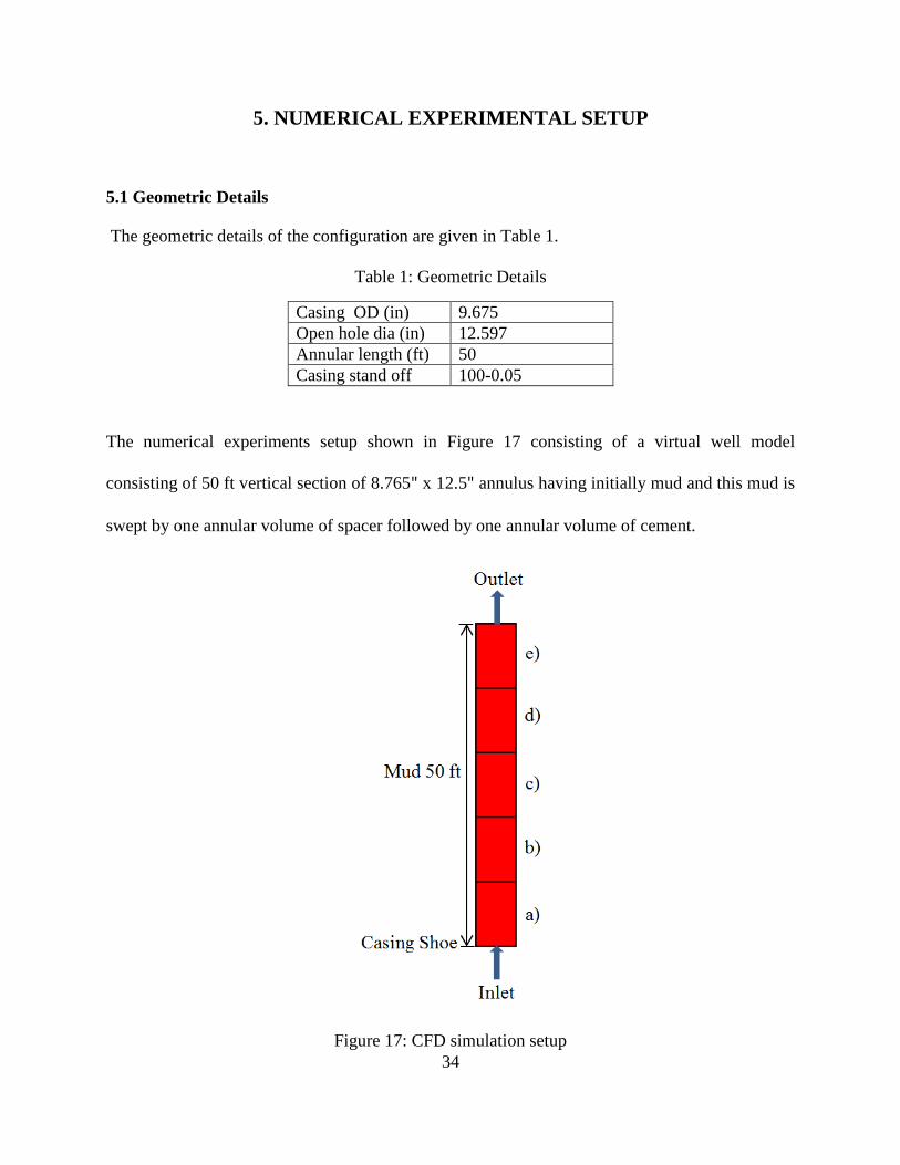
5. NUMERICAL EXPERIMENTAL SETUP .............................................................................. 34 5.1 Geometric Details ............................................................................................................... 34

5.1.2 Equivalent Sectional Annular Volume: ....................................................................... 35 5.1.3 Grid Details: ................................................................................................................. 35

5.2 Fluid, Boundary and Operating Conditions ........................................................................ 36 5.3 Details of Cases Studied ..................................................................................................... 39

6. SIMULATIONS RESULTS FOR VERTICAL CONFIGURATIONS ................................... 42

iv

6.1 Results with Spacer Density and Displacement Rate Variation ......................................... 43

6.2 Results for Spacer Viscosity and Displacement Rate Variations ....................................... 55 6.3 CFD Based Correlation ....................................................................................................... 65

6.3.1 Example Calculation Using Correlation ...................................................................... 67

6.4 Results with Eccentricity and Displacement Rate Variation .............................................. 69

7. HORIZONTAL WELL WITH VARIABLE ECCENTRICITY .............................................. 81 7.1 Introduction ......................................................................................................................... 81 7.2 Problem Setup ..................................................................................................................... 85

7.3 Cases Studied ...................................................................................................................... 88 7.4 Laminar Vs. Turbulent Flow Number Comparison ............................................................ 98 7.5 Same Flow Rate Different Fluids ....................................................................................... 99

8. SUMMARY AND CONCLUSIONS ..................................................................................... 101

REFERENCES ........................................................................................................................... 104

APPENDIX: CORRELATION DETAILS ................................................................................. 109

VITA ........................................................................................................................................... 111

v

LIST OF TABLES

Table 1: Geometric Details ........................................................................................................... 34

Table 2: Equivalent Sectional Annular Sweeps ............................................................................ 35

Table 3: Mud and Cement Rheological Properties ....................................................................... 37

Table 4: Spacer Fluid Properties Variations ................................................................................. 40

Table 5: Constants Obtained From Plots ...................................................................................... 66

Table 6: CFD and Correlation Data Comparison and Calculation of R2

Value ........................... 67

Table 7: Comparison of CFD and Correlation Values for Final Cement Volume Fraction ......... 68

Table 8: Casing Data ..................................................................................................................... 86

Table 9: Casing Deflection and Corresponding Eccentricity ....................................................... 87

Table 10: Fluids Data from a Case History - Malaysia ................................................................ 87

Table 11: Spacer Density and Viscosity Variation ....................................................................... 88

Table 12: Fluid 2 Rheological Data .............................................................................................. 99

vi

LIST OF FIGURES

Figure 1: Mud channel left on the narrow side of the annulus (Macondo incident-Chief Counsel’s

report, 2011). ................................................................................................................................... 4

Figure 2: Mud contamination effects on slurry properties and compressive strengths (data taken

from Abdel-Alim H. El-Sayed, 1995)............................................................................................. 7

Figure 3: The Macondo blowout (http://www.theatlantic.com/technology/archive/2010/10) ....... 8

Figure 4: Growth of Rayleigh Taylor instability (http://math.lanl.gov/) ...................................... 11

Figure 5: a) Equilibrium position and b) perturbed position of interface ..................................... 12

Figure 6: Finger shaped intrusion (http://harp.njit.edu/~kondic/capstone/2002/a/capstone.html) 14

Figure 7: Control volume discretization of a horizontal casing with variable eccentricity .......... 21

Figure 8: Typical sequence of a CFD simulation ......................................................................... 22

Figure 9: Interfacial reconstruction (piecewise-linear) scheme .................................................... 25

Figure 10: Schematic of locations for data comparison: .............................................................. 29

Figure 11: W* comparison for e = 0, 0.5, and 0.75 for Re = 220 ................................................. 30

Figure 12: Displacement efficiency e = 0, Re =220 ..................................................................... 30

Figure 13: Displacement efficiency e = 0.5, Re =220 .................................................................. 31

Figure 14: Displacement efficiency with positive density difference of 16% .............................. 31

Figure 15: Mud-Cement interface movement on a surface just above the casing wall on the

narrow side of the annulus at a) 1st annular flow, b) after 2

nd annular flow, c) after 3

rd annular

flow, d) after 4th

annular flow for eccentricity =0.5...................................................................... 32

Figure 16: Mud-Cement interface movement on a plane just above the casing wall on the narrow

side of the annulus at a) 1st annular flow, b) after 2


rd annular flow, d)

after 4th

annular flow for eccentricity =0.75 ................................................................................. 33

Figure 17: CFD simulation setup .................................................................................................. 34

Figure 18: A view of 2D axi-symmetric grid to highlight the grid clustering near walls ............. 36

Figure 19: The Power law profile and apparent viscosity variation of mud and cement ............. 38

vii

Figure 20: Frictional pressure drop of fluids with varying Reynolds number:............................. 39

Figure 21: Mud contamination indicator ...................................................................................... 42

Figure 22: Left over mud fraction in different sections for the case 1 ......................................... 43

Figure 23: Fluids fractions in sections (a, b, c, d, and e) for case 1 after one complete sweep .... 44

Figure 24: Instantaneous volume fraction plots for the case 1 ..................................................... 46







Figure 31: Left over mud fraction in different sections for the case 5 ........................................ 52

Figure 32: Instantaneous fluid fractions in sections (a, b, c, d and e) for case 5 after one sweep 53


Figure 34: Spacer volume fraction in the observation section just before cement breaks through

in the observation sections for all of the cases 1,2,3,4 and 5 ........................................................ 54

Figure 35: Cement volume fraction at different Reynolds numbers and densities ....................... 55


Figure 37: Volume fraction contour of fluids after one complete annular sweep ........................ 57


Figure 39: Left over mud fractions in different sections for the case 8 ........................................ 59


Figure 41: Left over mud fractions in different sections for the case 9 ........................................ 60


viii

Figure 43: Left over mud fractions in different sections for the case 10 ...................................... 62

Figure 44: Volume fraction of fluids after one complete annular sweep for case 10 ................... 63

Figure 45: Instantaneous volume fraction plots for the case 10 increasing displacement rate ..... 63

Figure 46: Cement volume fraction at different Reynolds numbers and viscosities .................... 64

Figure 47: Cement volume fraction after one annular flow over the entire length ....................... 65

Figure 48: Section view of concentric case with hexahedral cells ............................................... 69


Figure 50: Instantaneous fluid volume fraction in different sections for the case 11 ................... 71


Figure 52: Left over mud pattern comparison for e = 0.25 on a plane showing the wider and

narrow gaps and at four radial planes ........................................................................................... 73







Figure 59: Fluid volume fraction in different section for the case 15 .......................................... 78


Figure 61: Instantaneous mud volume fraction comparison cases 11,12,13,14 and 15 ................ 79

Figure 62: Fluid volume fractions in the reporting section after one annular flow for lighter

preflush followed by heavier spacer ............................................................................................. 80

Figure 63: Depiction of typical horizontal well cross section ...................................................... 82

Figure 64: Beam supported on its ends with uniform force distribution ...................................... 85

ix

Figure 65: Sections for leftover mud analysis .............................................................................. 88

Figure 66: Geometric of e = 0.15 .................................................................................................. 88

Figure 67: Leftover mud fraction for the cases 1, 2, 3 and 4 with e=0.15, Re=3304 ................... 89

Figure 68: Instantaneous fluid volume fraction plots for all the sections for the cases 1, 2, 3 and 4

with e=0.15, Re=3304 ................................................................................................................... 90

Figure 69: Fluid volume fraction contour on an axial and three radial planes towards the exit ... 91

Figure 70: Streamline plot colored by mixture volume fraction after one complete sweep ......... 92

Figure 71: Geometry with e = 0.30 ............................................................................................... 92

Figure 72: Leftover mud fraction for the cases 1, 2, 3 and 4 with e=0.3, Re=3304 ..................... 93

Figure 73: Instantaneous fluid volume fraction plots for all the sections for the

cases 1, 2, 3 and 4 ......................................................................................................................... 94

Figure 74: Fluid volume fraction contour on an axial and three radial panes towards the exit ... 94

Figure 75: Streamline plot colored by mixture volume fraction after one complete sweep ......... 95

Figure 76: Geometry with e =0.6 .................................................................................................. 95

Figure 77: Leftover mud fraction for the cases 1, 2, 3 and 4 with e=0.6, Re=3304 ..................... 96

Figure 78: Instantaneous fluid volume fraction plots for all the sections for the

cases 1, 2, 3 and 4 ......................................................................................................................... 96

Figure 79: Fluid volume fraction contour on an axial and three radial planes at maximum

deflection point at the center ......................................................................................................... 97

Figure 80: Fluid volume fraction contour on an axial and three radial planes towards the exit ... 97

Figure 81: Streamline plot colored by mixture volume fraction over entire domain ................... 98

Figure 82: Instantaneous volume fraction plot for e = 0.6 for laminar and turbulent flows ......... 99

Figure 83: Instantaneous volume fraction plot for e = 0.6 for fluid 1 & 2 ................................. 100

Figure 84: Plots for spacer density, viscosity and Reynolds number variations ........................ 110

x

NOMENCLATURE

Di Borehole diameter

Do Casing outer diameter

E Modulus of elasticity

I Moment of inertia

ρs Density of spacer

ρpf Density of pre-flush

ρm Density of mud

ρc Density of cement

Re Reynolds Number

τ Time for one annular sweep

μs Viscosity of spacer

μm Viscosity of mud

μc Viscosity of cement

μp Plastic viscosity

τy Yield stress

W* Peak to average velocity ratio

e Eccentricity

φc Volume fraction of cement

xi

ABSTRACT

Effective zonal isolation during primary cementing is only possible when drilling mud in the

annulus is completely displaced with cement, while the spacers aid in this process. During the

displacement process the rheological properties of fluids used and the operating conditions

control the motion of different fluids interfaces; desired stable interfacial displacement leads to

piston like motion.

Computational Fluid Dynamics (CFD) tool with the Volume-of-Fluid (VOF) has been validated

against experimental and used to conduct numerical experiments in a virtual well model

consisting of 50 ft vertical section of 8.765" x 12.5" annulus having initially mud and this mud is

swept by one annular volume of spacer followed by one annular volume of cement. The 50 ft

section was further divided into five subsections each of length 10 ft and average values of

quantities for these sections were used for further analysis. The mud and cement properties were

kept constant and the spacer density, viscosity and displacement rate were the only controlling

parameters to achieve the piston like displacement. The spacer density and viscosity were varied

between water and cement with cement being the heaviest and most viscous fluid. Three

Reynolds numbers of 100, 167 and 400 were simulated. Temporal variation of the mud volume

fraction was used as an indication for the piston like interfacial displacement. For an ideal piston

like interfacial displacement the mud fraction reduces sharply with minimum residual mud

volume after the spacer sweeps through. A gradual mud reduction represents fluid fingering and

the fluctuations in the mud fraction represent fluid mixing.

The best displacement was observed when the spacer had the same density as mud while it has

the viscosity similar to water. The displacement process was least effective when the spacer had

xii

the density equal to cement for all viscosity ranges. Based on the simulation results, a correlation

was developed to find the final placed cement volume fraction in the annulus under similar fluid

conditions, the utility of CFD based correlation is also presented. Further development of the

correlation for varying spacer volume at other operating conditions may be needed to extend its

applicability.

1

1. INTRODUCTION

1.1 Introduction

The most important and difficult objective to achieve during primary cement job is to provide

downhole zonal isolation, that is to ensure that no fluid movement is possible through the annular

cement sheath between different permeable zones located behind the casing. This requires that

the drilling mud originally present in the annulus be completely removed and replaced by cement

slurry, and that the cement, once set, reaches and retains over extended periods of time certain

mechanical properties such as bonding, compressive strength and permeability.

Incomplete mud displacement can leave a continuous mud channel across the zones of interest

that can lead to interzonal communication. Cement seal and bonding are also related to the

efficiency of the displacement process. Due to its importance mud displacement process has been

a topic of interest for such a long time in the well cementing community. Research concerning

the cement placement process began in 1930s. Some key factors influencing primary cement job

failures were identified, and solution were proposed as early as 1940. Using a large scale

simulator, Jones and Berdine (1940) showed that poor zonal isolation could be attributed to

channeling of the cement slurry through the mud. The presence of residual mud cake at the

cement/formation interface was also identified as a cause of poor mud displacement. To

minimize cement channeling, Jones and Berdine (1940) proposed to centralize the casing. They

also found the effective ways to remove the mud cake, including fluid jets, scrapers and

scratchers, casing reciprocation, and possibly pumping acid ahead of the cement slurry. Some of

these techniques are used in filed practice to remove the mud cake attached to the walls of the

well and casing.

2

Although researchers have tried to investigate the detailed mud displacement phenomenon, yet a

correlation describing the dependence of mud displacement efficiency on various contributing

parameters remains elusive.

During a cementing job, the cement slurry must displace all of the drilling mud from the

annulus. However, contact between the drilling mud and cement slurry often results in the

formation of an unpumpable viscous mass at the cement/drilling mud interface (Smith,

1984; Sauer, 1987). Under such circumstances, the drilling mud and the cement slurry are said to

be incompatible.

When incompatibility exists between fluids being displaced in the annulus, the displacing

fluid (i.e., the cement slurry) tends to channel through the viscous interfacial mass, leaving

patches of contaminated mud sticking to the walls of the casing and formation. This may

lead to insufficient zonal isolation, necessitating expensive remedial cementing prior to

stimulation treatment of the formation. The very viscous cement/mud mixture can also cause

unacceptably high friction pressures during the cement job, with the obvious danger of fracturing

a fragile formation. In extreme cases, total plugging of the annulus can occur, preventing

the completion of the cement job.

To avoid such problems one or more intermediate fluids (or preflushes), which are

compatible with both the cement slurry and drilling mud, are often pumped as a buffer to

prevent or at least minimize contact between them. Preflushes, pumped into the borehole in

front of the cement slurry, are designed to clean the drilling mud from the annulus and

leave the annular surfaces receptive to bonding with the cement. Thus, they must

eliminate the mud from the casing and formation walls (Sauer, 1987). To accomplish all

3

of these tasks, the rheological and chemical properties of preflushes must be carefully

designed.

1.2 Factors Affecting the Primary Cement Job

Many years of research have resulted in the following fundamental best practices

related to help optimize mud-displacement efficiency:

a) Condition of the drilling fluid (gel strengths).

b) Casing vs. hole size (annular cement sheath thickness).

c) Casing centralization/standoff.

d) Pipe movement (reciprocation and/or rotation).

e) Flow rates.

f) Formation permeability

g) Density difference between displacing and displaced fluid

h) Spacer design

i) Contact time.

a) Conditioning the mud i.e., to modification of its properties, prior to placing cement in the

wellbore greatly increases the displacement efficiency. Two mud characteristics cans be

changed- density and rheology. Anticipating the best conditions for displacement, it is desirable

to reduce the mud density to the minimum wellbore density limit (Beirute et al., 1991). Reducing

the mud’s gel strength, yield stress, and plastic viscosity is recognized as being very beneficial,

because the driving force necessary to displace the mud are reduced, and its mobility is

increased. Proper mud conditioning before cementing any well is probably the most important

factor affecting the success of the cement job and has been the topic of research and study for

4

years. Mud properties such as plastic viscosity, yield point, fluid loss, and gel strength

development should be optimized prior to drilling through areas to be cemented to prevent

excessive filter cake build up and pockets of highly gelled mud. Mud conditioning times

prior to cementing should approach or exceed three hole volumes or until the properties of the

mud pumped into the well equals that of the mud exiting the well (Crook et al., 1987).

b) Annular cement sheath thickness should be considered as part of the casing centralization

in that a minimum sheath thickness of 0.75 in. is recommended as a low range with an

optimal range of sheath thickness of 1.5 inches with proper centralization or standoff

requirements of a minimum of 70%. For a particular well in question, the optimum values for

these parameters should, however be calculated from programs that consider cement slurry

placement and cement sheath integrity (Llseng et al., 2005).

c) Centralization is a major problem in horizontal wells especially when the clearance is low.

Figure 1: Mud channel left on the narrow side of the annulus (Macondo incident-Chief Counsel’s

report, 2011).

5

Narrow annular clearance may require an even greater standoff percentage in order to provide a

sufficient flow path for flow to occur throughout the entire annulus and to prevent

accumulation of low-side mud solids (Keller et al., 1987). Centralizers are used to keep the

casing in the center of the hole, in addition the centralizers are useful in keeping the casing away

from borehole wall so that it does not stick to highly permeable zones (Mason et al., 1997).

d) Pipe movement, either rotation or reciprocation, is a major driving for mud removal. Both

movements are thought to be helpful in mobilizing the slowly moving or even static mud present

on the narrow side of an eccentric annulus Moroni (2009). When used in combination of

scratchers or scraopers, casing movement also shown to mechanically erode the mud cake, and

cosiderably improve the displacement process. This pipe movement, even though more

difficult in horizontal wells, should be attempted when possible (McPherson , 2000).

Studies have shown that pipe movement is beneficial not only in helping remove mud from

the low side of the annulus but in removing deposited drill solids during circulation in

combination with pipe movement. The additional mechanical agitation helps break up areas

of highly gelled mud and dislodges cuttings trapped in combination with mud filtercake

which may prevent the cuttings from being removed with fluid circulation alone.

e) Flow rates achieved during the circulation stage before and during the cementing and

displacement stage have a significant effect on mud displacement. The turbulent flow is the

most beneficial flow regime for improving displacement efficiencies (Sauer, 1987). Low

viscosity spacers in turbulence have been reported to aid in the removal of settled solids if

sufficient volume is used.

f) The presence of a mud cake at the wall of permeable formations is another factor which affects

the circulation process. When mud is not flowing across a permeable zone, it is subjected to

6

static filtration. Without sufficient fluid-loss control, an excessively thick filter cake can grow

and reduce the size of the annulus. Predicting how much mud cake will be eroded when flow is

resumed is difficult, because most mud cakes are compressible, and their characteristics vary as a

function of distance from the formation. The loose cake furthest from the wall can most probably

be eroded by the flow, but removal of the hard cake against the formation is much more difficult

(Reiley et al., 1987). There is a possible synergism between mud filtration and pipe eccentricity,

which would be detrimental to the circulation process. Since the erosion of the deposited filter

cake is an increasing function of the shears stress at the formation wall, the mud-cake thickness

during circulation is likely to be largest at the narrow side of the annulus.

g) Gravity forces, produced by a density difference between the two fluids, influence the

breakdown of gel structure of the drilling fluid and, therefore, may enhance displacement

efficiency. If the mud is lighter than the displacing fluid, buoyancy contributes to the displacing

process. The buoyant force is additive to the flow forces and displacement is easier than when

densities are equal.

h) The purpose of the spacer system is to serve as a mud removal aid and serve as a buffer

between the well fluids and the cement slurry (Kettle et al., 1993). The spacer must therefore be

compatible with both drilling mud and cement. Any incompatibilities may cause extremely

viscous fluids to be formed, resulting in fluid channeling through the viscous mixture and

excessive friction pressure. In wells in which oil based muds have been used, the added concern

of leaving the casing and formation in a water-wet condition must be addressed. Many additives

and surfactants are now available to optimize the spacer design to meet the requirements of an

individual well. Optimal displacement efficiency is obtained when the spacer density is equal to

mud density and very low viscosity.

7

i) In vertical wells, research has shown that a minimum of 8 to 10 minutes of spacer contact time

at the maximum rate possible should be planned for (Sauer, 1987; Smith, 1991). In horizontal

wells, contact time may need to be increased if any settled solids or excessive eccentricity is

expected. Additional spacer volume may aid in mud removal from the low side of the bore-hole

in eccentric annuli. Contact time is most important when oil based mud are used. In that case

chemical based spacers are used to remove the greasy mud from walls and also leave a layer of

water on stuck mud to have a better cement bond with formation.

1.3 Mud Contamination

When cement comes in contact with the mud during the displacement process and some of mud

is mixed with cement, the cement slurry properties are badly affected. The phenomenon of mud

contamination becomes severe with hole deviation and with eccentric casing. The effect of mud

contamination on cement rheological properties and compressive strength are shown in Figure 2.

Figure 2: Mud contamination effects on slurry properties and compressive strengths (data taken

from Abdel-Alim H. El-Sayed, 1995)

8

1.5 Motivation, Hypothesis and Objectives

The spill due to Macondo blowout is the largest accidental marine oil spill in the history of the

petroleum industry.

Figure 3: The Macondo blowout (http://www.theatlantic.com/technology/archive/2010/10)

The Chief Counsel’s Report (2011) about the Macondo incident states that “The root technical

cause of the blowout is now clear: “The CEMENT that BP and Halliburton pumped to the

bottom of the well failed to isolate hydrocarbons in the formation from the wellbore—that is, it

did not accomplish zonal isolation.” It also states that “the fluid mechanisms of mud

displacement, gas flow, and other cementing phenomena are exceedingly complex.” The need

for better understanding of the complex cement placement process is the main motivation to

carry out this study. It must be noted that our research work started prior to the Macondo

incident and the published recommendations of the Chief Counsel’s Report.

http://assets.theatlantic.com/static/mt/assets/science/4586214076_f1c745ea74_z.jpg

9

It is hypothesized that if under optimal conditions the interfacial contacts or instabilities at the

different fluid interfaces (i.e. at cement-spacer and spacer-mud interfaces) can be prevented from

merging with each other during the entire displacement process, then the spacer would act as a

fluid plug, thus keeping the cement and mud separated and resulting in perfect mud sweep and

good cement job.

The main objectives of this numerical study are to understand the role of interfacial instabilities

in the primary cementing and try to quantify the performance of spacer in removing mud and

keeping mud and cement separated in cement-spacer-mud systems. The spacer performance is a

function of its volume, rheological properties of all of the fluids involved, displacement rate and

hole configuration. CFD simulation based correlations is to be developed to quantify the

displacement efficiency under various operating conditions.

10

2. LITERATURE REVIEW

2.1-Interfacial Instabilities

The stability of the interface between the two moving fluids has significant importance in many

petroleum engineering application such as primary cement placement and enhanced oil recovery.

In the case of primary cementing the major physical properties influencing the stability of the

interface is the density and viscosity ratios of the displacing and displaced fluids, while in

enhanced oil recovery there are other factors that have major contribution in determining a stable

interface like mobility ratio of fluids, heterogeneity of the medium, gravity segregation and

capillary pressure.

The instability of the interface between two superposed Newtonian fluids of different densities at

rest was initially studied by Rayleigh (1882). Taylor (1950) included the effect of a constant

acceleration acting perpendicularly to the interface and concluded that if the acceleration is

directed from the less dense to the denser medium then any slight disturbance to the interface

will grow exponentially with time. Subsequently, Bellman and Pennington [9] examined the

effects of surface tension and viscosity on this instability and discovered the presence of a

critical wave number with the property that the interface is stable or unstable depending on

whether the wave number is greater than or less than this critical wave number. Where non-

Newtonian fluids are concerned very little work has been done on this problem, even in the

linear case.

2.1.2 - Rayleigh Taylor Instability: The instability of the interface between two superposed

Newtonian fluids of different densities at rest was initially studied by Rayleigh (1882) in which

initially the heavier fluid was resting on lighter fluid.

11

Taylor (1950) included the effect of a constant acceleration acting perpendicularly to the

interface and concluded that if the acceleration is directed from the less dense to the denser

medium then any slight disturbance to the interface will grow exponentially with time, shown in

Figure 4.

Figure 4: Growth of Rayleigh Taylor instability (http://math.lanl.gov/)

A simple analytic model explaining the interfacial instabilities is presented by Piriz et al. (2006).

This model is based on the balance of forces. The model explains the physical mechanism that

drives the instability and can be extended to more complex situations without much extra

conceptual effort. In some cases, such as for viscous fluids, a simple approximation leads to an

explicit equation for the instability growth rate from which the physical effects of viscosity on

the instability evolution can be easily understood. The same approximation can be used for other

12

cases including non- Newtonian fluids and elastic solids, provided that an adequate constitutive

model is proposed.

The simplest case in which the Rayleigh-Taylor instability arises is for two semi-infinite

incompressible and inviscid fluids with a surface of contact initially at y = 0 as shown in

Figure 5(a). The denser fluid of density ρ2 lies above the lighter fluid of density ρ1 < ρ2 in a

uniform gravitational field g. If the interface between the fluids is initially perfectly planar and

equilibrium exists, the fluid elements on each side of the interface immediately above and below

must have the same pressure p1 = p2 = p0. Now, let us introduce a small perturbation ξ(x) at the

interface such that the elements originally at y = 0 are now translated to the new position y = ξ(x)

as shown in Figure 5(b). The pressure on each side of the translated fluid interface is

(1a)

(1b)

Figure 5: a) Equilibrium position and b) perturbed position of interface

In the new position, a pressure difference – is created across the interface,

which tends to deform it further. This pressure difference drives the motion of the interface. This

13

Motion can be described by Newton’s second law of motion

(2)

where A is the area of the interface and m is the mass of the fluids involved in motion. To

calculate this mass we assume that the Rayleigh-Taylor instability induces surface modes that

decay from the interface as exp (ky), where k =2π/λ is the wave number and λ is the wavelength

of the perturbation. That is, in the linear regime the intensity of the motion decays with the

distance from the interface with a characteristic length k−1.

Therefore the total effective mass that

participates in the motion is the mass contained within this distance,

(3)

where m1 and m2 are, respectively the masses of the light and heavy fluids that move with the

interface.

From Eq. (2) and (3) the equation of motion of the interface can be written as

(4)

or

(5)

Where

is the Atwood number. Integrating equation (5), we have

(6)

14

where 0 = (t=0) and are, respectively, the initial perturbation amplitude and

velocity of the interface, and √ is the asymptotic growth rate.

The extension of these arguments to more complex situations such as those involving non-ideal

fluids is straightforward and requires additional forces Fi on the interface that must be included

into the equation of motion. In general we can write

∑

Where Fi could be surface tension or viscosity effects.

2.1.3 Saffman-Taylor Instability: An interfacial instability occurs when a more viscous fluid is

displaced by the less viscous one, this instability is known as the Saffman-Taylor instability

(Saffman and Taylor 1958).

Figure 6: Finger shaped intrusion (http://harp.njit.edu/~kondic/capstone/2002/a/capstone.html)

This instability results in the form of finger-shaped intrusions of the displacing fluid into the

displaced one and can have significant impact on the efficiency of displacement process. When

15

the driving factor behind the instability is the viscosity ratio of the two fluids, the instability is

referred to as the viscous fingering instability shown in Figure 6.

Viscous fingering generally refers to the onset and evolution of instabilities that occur in the

displacement of fluids in a porous medium. The viscosity difference between the fluids is the

major factor for onset of these instabilities. The other factors that play an important role on the

onset of these instabilities are gravity and heterogeneity of the medium (not involved in this

case).

For any given set of conditions, all interfacial perturbations below a critical wavelength are

eliminated due to dispersion. Perturbations above the critical wavelength continue to grow at an

unfavorable mobility ratio. New fingers may initiate from the ends of already growing fingers.

The growth of the finger occurs both in length and in average width. In length, the finger growth

is approximately linear with time. Finger growth in width is a combination of spreading by

transverse dispersion, by merging and coalescence of smaller fingers into larger fingers Perkins

(1964).

As mentioned earlier that the contributing factors towards interfacial instabilities are density and

viscosity differences between displacing and displaced fluids. If we can control these parameters

and suppress the initiation and propagation of the instabilities, than we can have piston like

moving interface with maximum sweep efficiency.

2.2 Secondary Flow Instabilities

In an eccentric channel, where the displacing fluid has a tendency to channel through the wide

side, density difference produces a hydrostatic pressure imbalance between the wide and narrow

sides. This imbalance induces a secondary gravity-driven azimuthal current from the wide side

16

to the narrow side of the annulus. Regardless of eccentricity, density difference also induces

secondary radial flows across the annular gap. This is due to a hydrostatic pressure imbalance

between the central part of the annulus and regions near the walls. The relative strengths of the

azimuthal and radial currents depend on eccentricity and the rheology of the fluids. Under certain

conditions significant azimuthal instabilities occur which appear to accelerate displacement in

the narrow side of annulus. Intensity of azimuthal instabilities is related to flow rates and density

differences (Tehrani et al. 1993).

The interface between two miscible fluids with similar rheologies, but with different

densities, is stable so long as the denser fluid lies below the interface, and the interface

is not near vertical. When flow conditions are such that the interface becomes close to

vertical, small perturbations in the flow field may trigger gravity driven interfacial

instabilities.

When the azimuthal instabilities are severe, cement flows towards the narrow side through

formation of fingers branching away from the main axial flow. Since the motion of the fingers is

towards the narrow side, they move at a lower axial velocity than the main body of cement and

appear to be falling away at the interface. As the fingers cascade towards the narrow side,

streams of mud become trapped between the fingers and the main body of cement. These streams

are directed towards the wider part of the annulus and are carried away by the main body of

cement. In situations of high azimuthal instability, the falling fingers accelerate displacement in

the narrow side. However, in most cases a thin wavy strip of mud is left behind in the narrow

side. In addition, small pockets of mud may become trapped in the narrow side where they are

likely to remain indefinitely.

17

2.3 Previous Research Work In the Area of Mud Displacement

Research concerning the cement placement process began in 1930s. Some key factors

influencing primary cement job failures were identified, and solution were proposed as early as

1940. Using a large scale simulator, Jones and Berdine (1940) showed that poor zonal isolation

could be attributed to channeling of the cement slurry through the mud. The presence of residual

mud cake at the cement/formation interface was also identified as a cause of poor mud

displacement. To minimize cement channeling, Jones and Berdine (1940) proposed to centralize

the casing. They also found the effective ways to remove the mud cake, including fluid jets,

scrapers and scratchers, casing reciprocation, and possibly pumping acid ahead of the cement

slurry.

Howard and Clark (1948) first recognized the importance of the conditioning of the drilling

fluid. They concluded that a decrease in viscosity of the drilling fluid will increase displacement

efficiency. An extensive study on how pipe movement affects the displacement process was

performed by Mclean et al. (1967). They concluded that when casing is severely off center,

rotation tend to force the cement into bypassed mud. They also claim that if the pipe is well

centralized, reciprocation appears to be better choice.

Mclean et al. (1967) studied the effect of flow rate on removing the circulatable drilling fluid.

They concluded that channels of gelled mud lodged in the narrow crevices are reduced in size by

increasing the flow rate. Mclean et al. (1967) along with Howard and Clark (1948), report that if

mud is lighter than the displacing Fluid, buoyancy contributes to the displacement process. The

buoyant force is additive to the flow force and displacement is easier than when densities are

equal.

18

Haut and Crook (1979) studied the various factors that influence the mud displacement process.

They conducted various test with different combinations of cement and mud systems and

measured the displacement efficiencies.

The theoretical approach also has its limitations. The complete modeling of the displacement

process is really a difficult task, even for the most sophisticated computers. For example, one

must contend with unsteady mass and momentum transfer between non-Newtonian fluids of

different properties in an asymmetric geometry. Researchers have tried to simulate the mud

displacement by simplifying the process through assumptions.

Beirute and Flumerfelt (1977) studied the phenomenon by assuming that the leading edge of the

displacing fluid is well defined and stable, and that the flow is one-dimensional, having only an

axial velocity component only. Because of these very simplifying assumptions, it does not

provide a realistic picture of the phenomenon. Haut et al. (1978) in their computer simulation

investigation the relative importance of the various physical and rheological properties of the

fluids involved in a primary cementing. They found that difference in densities between drilling

fluid and cement was a major factor controlling displacement efficiency and the formation of the

interface. The simulator used in that study was limited to axi-symmetric flows only.

Due to geometric complexities and non-linearity of the shear stress-shear rate relationship of the

fluids involved, analytic solutions to the equations of motion in this type of flow are extremely

difficult. For axial flow in a narrow-width annulus, it is a well-known practice to neglect the

curvature. When the ratio of the radius of the inner pipe to that of the outer pipe is close to unity,

an eccentric annulus may be considered as a slot of variable width. Iyoho et al. (1981)

determined the velocity profile for a power-law fluid using this method. This approach has been

19

used by others to solve the problem of laminar displacement in an annulus, but these are

restricted mostly to displacements in a concentric annulus.

Tehrani et al. (1992) combined experimental and theoretical study of laminar displacement in an

inclined eccentric annulus. They used dynamic similarity to investigate the effects of different

variables on displacement. They concluded that, in general efficient laminar displacement

requires good centralization, a high density contrast (10 to 15% in terms of field conditions) and

a positive rheological hierarchy.

Frigaard and Pelipenko (1993) used Hele-Shaw approach, in which instead of solving

3-dimensional problem, involves the averaging across the annular gap and solving the

2-dimensional model. This scheme has the drawback of not addressing the possibility that mud

may remain static in layers stuck to the inner and outer walls of the annulus.

Guillot and Frigaard (2007) studied the efficiency of various preflushes in displacing mud. They

found that, preflushes may not be as effective as they are thought of in preventing direct contact

between the drilling fluid and the cement slurry, even when industry accepted rules are used to

design these preflushes.

20

3. NUMERICAL SETUP

The modeling of multi-phase flow is not an easy task, both from a physical and numerical point

of view. The complexity of the phenomenon arises from the presence of an interphase surface

(front, interface) on which physical properties change discontinuously (e.g. density, viscosity,

pressure). This surface may be considered as a moving boundary, where appropriate boundary

conditions must be imposed and an evolution of which needs to be found as a part of the

solution. In the case of immiscible non-reacting fluids, the interface is simply advected with the

velocity of the flow.

Many methods for tracking the interphase surface can be found in the literature. The most

popular of those are: the front tracking method (interface modeled as a set of connected

markers), the Level Set method (interface captured implicitly as the zero level set of a signed

distance function) and the Volume of Fluid method Youngs (1982).

3.1 Computational Fluid Dynamics (CFD) Technique

Computational fluid dynamics (CFD) is the science of predicting fluid flow, heat and mass

transfer, chemical reactions, and related phenomena by solving numerically the set of governing

mathematical equations, conservation of mass, momentum, energy, species, etc. Technique that

has been used in this study is based on finite volume method. In which domain is discretized

onto a finite set off control volumes (or cells), shown in Figure 7. General conservation

(transport) equations for mass, momentum, energy, species, etc. are solved on this set of control

volumes. The governing equations for the conservation of mass and momentum are explained in

the subsequent sections, as no temperature dependence was considered, therefore energy

equation was not solved in theses simulations.

21

The equation for conservation of mass for an infinitesimal control volume is shown below

It is often called the equation of continuity because it requires no assumptions except that the

density and velocity are continuum functions.

Figure 7: Control volume discretization of a horizontal casing with variable eccentricity

The following set of momentum balance equations for Newtonian fluids on the control volume

cell is called Navier Stokes equations after C. L. M. H. Navier (1785–1836) and Sir George G.

Stokes (1819–1903), who are credited with their derivation.

(

)

(

)

(

)

22

These equations four unknowns: ρ, u, v and w. These should be combined with the continuity

relation to form four equations in these four unknowns.

These partial differential equations are discretized into a system of algebraic equations. All

algebraic equations are then solved numerically to render the solution field. Typical sequence of

CFD simulation is shown below in Figure 8. First sold model is built and a mesh is generated

and fed to the solver, depending on the physics of the model being involved physical model is

selected with appropriate boundary and initial conditions and fluid properties. Then results are

analyzed during post processing step.

Figure 8: Typical sequence of a CFD simulation

3.2 Volume of Fluid Method

The volume-of-fluid method Youngs (1982) tracks the volume of each fluid in all cells

containing portions of the interface, rather than the interface itself. The VOF formulation relies

23

on the fact that two or more fluids (or phases) are not interpenetrating. In each control volume,

the volume fractions of all phases sum to unity. The fields for all variables and properties are

shared by the phases and represent volume-averaged values, as long as the volume fraction of

each of the phases is known at each location. Thus the variables and properties in any given cell

are either purely representative of one of the phases, or representative of a mixture of the phases,

depending upon the volume fraction values. In other words, if the qth

fluid’s volume fraction in

the cell is denoted as αq, then the following three conditions are possible:

αq = 0: The cell is empty (of the qth

fluid).

αq = 1: The cell is full (of the qth

fluid).

0 < αq<,1: The cell contains the interface between qth

the fluid and one or more other

fluids.

Based on the local value of αq, the appropriate properties and variables will be assigned to each

control volume within the domain (Fluent user’s guide).

The VOF method solves a non-diffusive solution of the advection equation, by a geometrically

based calculation technique of the void fraction fluxes at the cell faces based on the

reconstructed interface Afshin (2008).

The tracking of the interface(s) between the phases is accomplished by the solution of a

continuity equation for the volume fraction of one (or more) of the phases. For the phase,

this equation has the following form (Fluent user’s guide).

24

( )

∑

Where is the mass transfer from phase q to phase p and is the mass transfer from phase

p to phase q. is the mass source term. The volume fraction equation will not be solved for the

primary phase; the primary-phase volume fraction will be computed based on the following

constraint:

∑

The properties appearing in the transport equations are determined by the presence of the

component phases in each control volume. In a two-phase system, for example, if the phases are

represented by the subscripts 1 and 2, and if the volume fraction of the second of these is being

tracked, the density in each cell is given by

In general, for an n-phase system, the volume-fraction-averaged density takes on the following

form:

∑

All other properties (e.g., viscosity) are computed in this manner.

A single momentum equation is solved throughout the domain, and the resulting velocity field is

shared among the phases. The momentum equation, shown below, is dependent on the volume

fractions of all phases through the properties ρ and μ.

25

Where F stands for body forces, g for gravity acceleration, and p for pressure.

One limitation of the shared-fields approximation is that in cases where large velocity

differences exist between the phases, the accuracy of the velocities computed near the interface

can be adversely affected. Note that if the viscosity ratio is more than 1 x 103, this may lead to

convergence difficulties (Fluent user’s guide).

3.3 Interfacial Reconstruction Scheme

When the cell is near the interface between two phases, the geometric reconstruction scheme is

used (Fluent user’s guide). The geometric reconstruction scheme represents the interface

between fluids using a piecewise-linear approach shown in Figure 9. It assumes that the interface

between two fluids has a linear slope within each cell, and uses this linear shape for calculation

of the advection of fluid through the cell faces.

Figure 9: Interfacial reconstruction (piecewise-linear) scheme

The first step in this reconstruction scheme is calculating the position of the linear interface

relative to the center of each partially-filled cell, based on information about the volume fraction

and its derivatives in the cell. The second step is calculating the advecting amount of fluid

26

through each face using the computed linear interface representation and information about the

normal and tangential velocity distribution on the face. The third step is calculating the volume

fraction in each cell using the balance of fluxes calculated during the previous step.

27

4. VALIDATION AND VERIFICATION

For validation study, experimental results of Tehrani et al. (1993) have been used. In these

experiments, they used conductivity probes to measure the displacement efficiency of mud and

annular velocity profiles at a specified location. They carried out these experiments for both

concentric and eccentric annulus with single fluid as displacing and displaced fluid, they varied

the fluid displacement rates and conducted one case with a density difference of 16% between

the displacing and displaced fluids. The experimental setup consisted of two coaxial cylindrical

tubes. The ID and OD of the annulus are 1.5748 inches and 1.9695 inches respectively, creating

a concentric gap of 0.19685 inches. The total axial length of the tubes was 9.843 ft.

4.1 Reynolds Number Calculation Herschel Bulkley Model

The procedure adopted for Reynolds number calculation is taken from (Antonino Merlo et al.

1995) and is described below. The equivalent Reynolds number in the annulus is given by the

following expression

Where

{

[(

) (

)]

}

28

{[

] [

(

)]}

[

] [

(

)]

(

)

R2 is hole radius, R1 casing outer radius and Va is the average velocity of fluid. After substituting

the values of Ca and Re, the final form of equivalent Reynolds number is

(

)

(

)

( )

In filed units this expression becomes

(

)

(

)

(

)

( )

Critical Equivalent Reynolds Number is given by the following equation:

[

]

Where

29

For Reeq< Reeqcr the flow is considered laminar while for Reeq> Reeqcr the flow becomes

turbulent.

4.2 Results for Same Density Fluids

Commercially available CFD code based on unstructured finite volume formulation of Non-

Newtonian Navier-Stokes equations is used for all the simulations performed in this research

study (Fluent, user’s guide). Volume of Fluid method (VOF) is used in this study to track the

fluid interfaces Youngs (1982). The most commonly used parameter for defining the ability of a

given fluid to displace another is the displacement efficiency. At any time t > 0, it is defined as

the fraction of annular volume occupied by the displacing fluid (cement), if all the annular

volume is occupied by displacing fluid then displacement efficiency is 1. Typical values of

rheological parameters for experimental setup were: τy = 1.22 Pa, k = 0.197 Pa Sn

and n = 0.505.

W* is the ratio of peak axial to average axial velocity in the annulus at is reported at 0.75L,

where L is the total axial length of the annuals. Locations for data comparisons are schematically

shown in Figure 10.

Figure 10: Schematic of locations for data comparison:

ro ri

90°

0° 180

°

0.25L

0.75L

L=9.843’

Inlet

Outlet

30

W* comparison for e = 0, 0.5 and 0.75 with experimental results shown in Figure 11 have good

agreement with the experimentally measured values, thus validating the computational model

and simulation tool. An interesting way to look at the above plots, is the region of the plot where

W* is nearly zero, meaning that the mud is static in this region.

Figure 11: W* comparison for e = 0, 0.5, and 0.75 for Re = 220

Comparison of the calculated values for the displacement efficiency and experimental measured

value for eccentricity zero is shown in Figure 12. CFD simulations not only follow the same

trend but also the numbers are in reasonable agreement with the experimental.

Figure 12: Displacement efficiency e = 0, Re =220

31

For eccentric cases it can be seen the CFD results match very well with the experimental data up

to two annular volume flows, however small deviations are observed on later times with CFD

results over predicting the experimental data. It should be noted that the focus of this study is the

first annular volume sweep that remains in good agreement with experimental data.

Figure 13: Displacement efficiency e = 0.5, Re =220

4.3 Results with Positive Density Difference between Fluids

The positive density difference improves the displacement efficiency, a comparison of CFD and

experimental results are shown in Figure 14, the match for density differences is also reasonable.

Figure 14: Displacement efficiency with positive density difference of 16%

32

For qualitative insight, the contours of mud volume fraction on the lower portion of narrower

side of annulus are shown in Figure 15 (qualitative experimental results were not available to

compare). It can be seen that for the given flow conditions, the volume of the trapped mud on the

narrow side does decrease, and the lowest location of mud adhering the wall surface is displaced

upward with increasing annular flows.

a)

b)

c)

d)

Figure 15: Mud-Cement interface movement on a surface just above the casing wall on the

narrow side of the annulus at a) 1st annular flow, b) after 2


rd annular

flow, d) after 4th

annular flow for eccentricity =0.5.

0.164 ft

0.5 ft

0.5 ft

0.5 ft

0.5 ft

0.5 ft

Mud

Cement

33

The problem of trapped mud for higher eccentricity of 0.75 becomes worse. Contours of trapped

mud volume fractions for eccentricity of 0.75 are shown in Figure 16, it can be observed that

even after four annular flows the mud layer on narrow side of the annulus is barely moved

upward.

a)

b)

c)

d)

Figure 16: Mud-Cement interface movement on a plane just above the casing wall on the narrow

side of the annulus at a) 1st annular flow, b) after 2


rd annular flow, d)

after 4th

annular flow for eccentricity =0.75

0.5 ft

0.5 ft

0.5 ft

0.5 ft

0.5 ft

34

5. NUMERICAL EXPERIMENTAL SETUP

5.1 Geometric Details

The geometric details of the configuration are given in Table 1.

Table 1: Geometric Details

Casing OD (in) 9.675

Open hole dia (in) 12.597

Annular length (ft) 50

Casing stand off 100-0.05

The numerical experiments setup shown in Figure 17 consisting of a virtual well model

consisting of 50 ft vertical section of 8.765" x 12.5" annulus having initially mud and this mud is

swept by one annular volume of spacer followed by one annular volume of cement.

Figure 17: CFD simulation setup

35

The annulus is divided into five sections (a, b, c, d, e) of equal length of 10 ft. Each 10 ft section

has 10 observation sections where the values of volume fraction of each fluid are taken and

averaged over that section.

5.1.2 Equivalent Sectional Annular Volume: The displacement process in the sections a, b, c,

d and e can also be looked individually in each section as well as combined annular sweep in the

entire 50 ft annulus. In this way the entire sweep of cement from inlet to outlet can be divided

into the equivalent sectional annular sweeps. For example when the cement front reaches the first

section (a), then this section has already been swept five times by the spacer as spacer has

originally annular length of 50 ft and section (a) has annular length 10 ft. Based on the average

cement velocity when its one annular volume has been pumped, then according to the above

argument, the spacer and cement sweeps for each section are shown in Table 2. The results in

the next chapters will be based on this equivalent sectional approach and temporal dependence of

volume fraction of each fluid in the section (e) to see the effect of interfacial instabilities in terms

of the integrity of the spacer.

Table 2: Equivalent Sectional Annular Sweeps

Section Spacer Equivalent

Annular Sweeps

Cement Equivalent

Annular Sweeps

a 5 5

b 5 4

c 5 3

d 5 2

e 5 1

5.1.3 Grid Details: For concentric cases 2D axi-symmetric approximation was used, sectional

view is shown in Figure 18. Grids having quadrilateral cells were created with 36000 (1715 axial

x 21 radial) cells. Sufficient clustering towards walls was applied to resolve the gradients in

those regions while in the axial direction the grid points were uniformly distributed. These

36

dimensions were selected based on the fluids involved and displacement rates that were to be

studied in the set of simulations that were to be performed. These dimensions were more than the

minimum needed dimensions in terms of grid independence and for log law applications if

turbulence model were to be used. Based on this radial cell distribution the wall y+ values were

in the range of 5-10, more than the required of 30-60.

Figure 18: A view of 2D axi-symmetric grid to highlight the grid clustering near walls

5.2 Fluid, Boundary and Operating Conditions

Inlet: velocity inlet

Outlet: Outflow

Wall: No slip adiabatic, smooth pipe

Fluid Rheology: Power law (Vertical Concentric) and Herschel Bulkley (Vertical eccentric and

horizontal)

Fluids Interaction: Immiscible (no interfacial tension)

Operating Temperature and Pressure: Atmospheric

Temperature: No temperature effects

Compressibility: Incompressible fluids

Chemical reaction: No chemical reactions

37

Fluids in majority of the cases studied were treated as power law fluids. The Reynolds number

and apparent Newtonian viscosity were calculated by the following expressions Bourgoyne etal.

(1986)

[

]

(

⁄

)

Where v is the average velocity (ft/s), d2 is the borehole dia, d1 is the casing outer dia, n and k are

power law exponent and consistency index respectively and can be calculated by

The typical mud and cement properties and ranges were taken from Wilson and Sabins (1998)

and are shown in Table 3. During the entire flow simulations the cement and mud fluid

properties were kept constant.

Table 3: Mud and Cement Rheological Properties

Fluid Density

(lbm/gal)

Plastic

Viscosity

(cp)

Yield

Point

(lbf/100ft2)

Power Law

Exponent

(n)

Consistency

Index K (eq.

cp)

Mud 13.1 63 53 0.607 1346

Cement 15.8 15 48 0.308 4708

38

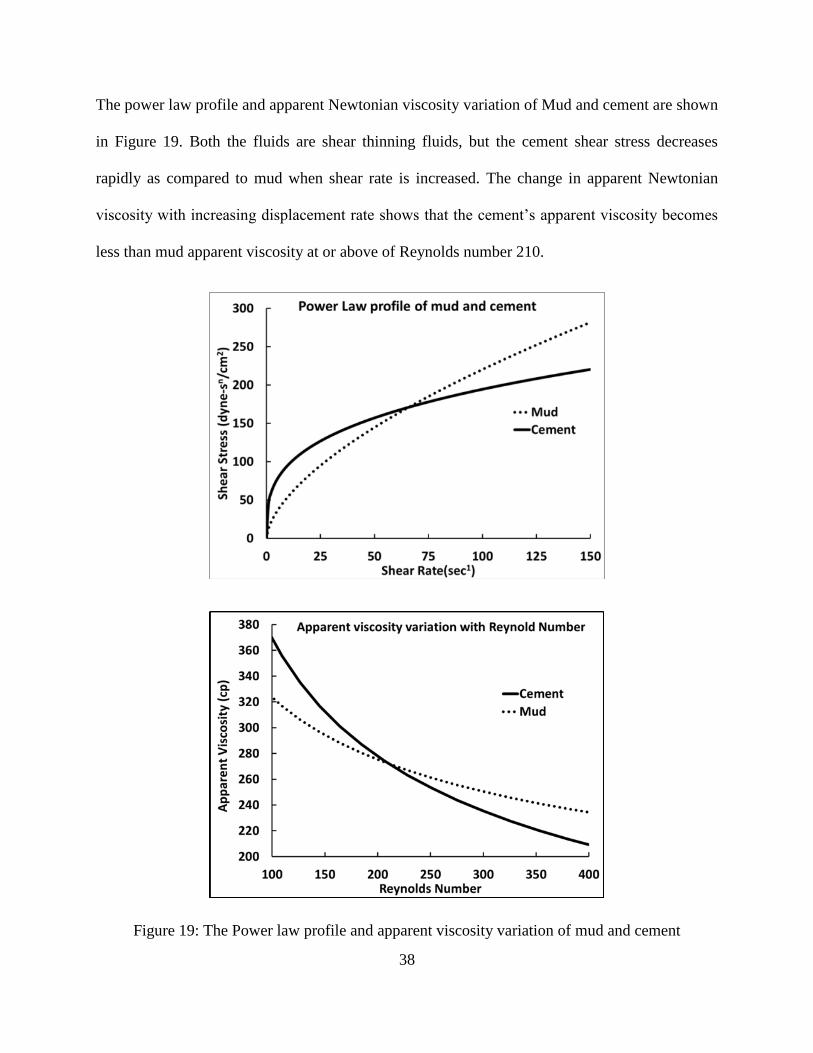
The power law profile and apparent Newtonian viscosity variation of Mud and cement are shown

in Figure 19. Both the fluids are shear thinning fluids, but the cement shear stress decreases

rapidly as compared to mud when shear rate is increased. The change in apparent Newtonian

viscosity with increasing displacement rate shows that the cement’s apparent viscosity becomes

less than mud apparent viscosity at or above of Reynolds number 210.

Figure 19: The Power law profile and apparent viscosity variation of mud and cement

39

The frictional pressure drop with increase of Reynolds number is shown in Figure 20. Cement

due to its low viscosity as compared to mud after Reynolds number 210 have less frictional

pressure drop as compared to mud, while before reaching the Reynolds number of 210 cement

was having more frictional drops as compared to mud.

Figure 20: Frictional pressure drop of fluids with varying Reynolds number:

5.3 Details of Cases Studied

Spacer density was varied between fresh water and cement densities, shown in Table 4 . Due to

the field applications of fresh water as spacer and in the case of narrow margin between the

formation pressure and formation fracture gradient, the limits for the spacer density were defined

as that of fresh water density as minimum and cement density as maximum. For the density

variations the spacer densities are equal to that of water, average of water and mud, equal to

mud, average of mud and cement and equal to that of cement. Note that cement density is greater

than mud density in all of these simulations.

40

Table 4: Spacer Fluid Properties and Displacement Rate Variations for Vertical Well Cases

Case # e ρs (lbm/gal)= μs (Cp)=

Spacer

Combination Re

Spacer

(ft)

Preflush

(ft)

1 0 ρw =8.33 μw =1 50 0 100,167,400

2 0 (ρw + ρm)/2=10.72 μw =1 50 0 100,167,400

3 0 ρm=13.11 μw =1 50 0 100,167,400

4 0 (ρm + ρc)/2=14.46 μw =1 50 0 100,167,400

5 0 ρc=15.81 μw =1 50 0 100,167,400

6 0 (ρm + ρc)/2=14.46 μw =1 50 0 100,167,400

7 0 (ρm + ρc)/2=14.46 (μw+ μm)/2=138,130,118 50 0 100,167,400

8 0 (ρm + ρc)/2=14.46 μm=324,287,234 50 0 100,167,400

9 0 (ρm + ρc)/2=14.46 (μm+ μc)/2=345,293,221 50 0 100,167,400

10 0 (ρm + ρc)/2=14.46 μc=368,298,209 50 0 100,167,400

11 0.05 ρm=13.11 μw =1 50 0 100,167,400

12 0.25 ρm=13.11 μw =1 50 0 100,167,400

13 0.5 ρm=13.11 μw =1 50 0 100,167,400

14 0.75 ρm=13.11 μw =1 50 0 100,167,400

15 0.95 ρm=13.11 μw =1 50 0 100,167,400

16 0 ρm=13.11 μw =1

49 1

400

45 5

40 10

25 25

20 30

10 40

Please note that each case is run for three different Re of 100,167,400 and the case number was

assigned according to the fluid property variation. For spacer viscosity the minimum limit was

taken as fresh water viscosity and maximum as cement, because cement was the most viscous

fluid in this set of data. For the cases in which spacer viscosity was varied, the spacer was taken

as Power law fluid and its power law exponent n and consistency index K were adjusted in such

a way that the spacer apparent viscosity was matched with water, mud and cement. For the cases

in which spacer has average values of viscosities like average of water and mud, for these cases

41

average values of n and K were taken and then K value was adjusted in such a way that the

required apparent viscosity of spacer was obtained.

For the cases 11-15 the casing eccentricity was varied from 0.05 to 0.95 in five steps and case

numbers were assigned according to eccentricity variations, the spacer density and viscosity

were kept constant; the values are shown in Table 4. Fluid rheology was modeled using

Herschel Bulkley fluid model.

A combination of lighter preflush followed by heavier spacer (total 50 ft) was also studied to see

their combined effect on the mud displacement efficiency. The combinations that were studied

are shown in Table 4. For this particular case L (Lighter) stands for annular length of preflush in

ft which in this case is water and H (Heavy) stands for annular length of spacer with density of

mud and viscosity of water. The Power Law rheological model was used.

42

6. SIMULATIONS RESULTS FOR VERTICAL CONFIGURATIONS

The results for the simulations are shown in three forms, one form is bar plot of unswept mud in

each annular section a, b, c, d and e, cement fraction is also shown alongside mud fraction

denoted by symbol φc. To quantify the unswept mud fraction in each of annular sections the ratio

of average mud volume fraction left in that section to the corresponding cement fraction is

defined in terms of mud contamination indicator. The colors assigned to the ratio of mud and

cement are shown in Figure 21.

Figure 21: Mud contamination indicator

To monitor the stability of different fluid interfaces, temporal data of volume fraction of each

fluid for the section (e) is plotted, section (e) was selected, because it is the last section towards

exit and the interface deformation can best analyzed in this section. With a stable interface any

fluid should be filling the most of the annulus. If the spacer keeps its integrity than upon its

breakthrough into section (e) its fraction should rapidly increase and in ideal case should reach to

1, correspondingly the mud fraction should rapidly decrease and should approach zero. Similarly

when cement breaks through in the section, its fraction should approach 1.0 rapidly and spacer

fraction should go to zero.

φm /φc ≤ 0.5

0.5< φm /φc < 0.1

φm /φc ≥ 0.1

43

6.1 Results with Spacer Density and Displacement Rate Variation

Case 1: The amount of left over mud in the first two sections (a) and (b) when fresh water was

used as a spacer is nearly zero for all the displacement rates studied and there is nearly 100%

cement in these two sections. Please note that at the instant of time when the data was taken five

equivalent sectional annular volume of spacer has already swept through all of the five sections

and cement has swept five times section (a), four times section (b), three times section (c), two

times section (d) and one time section (e) in terms of equivalent sectional annular volumes.

Figure 22: Left over mud fraction in different sections for the case 1

For the displacement rate corresponding to Reynolds number of 100, cement and mud fraction

nearly makes up the total volume in each section while with increase of displacement rate some

44

spacer is also left over in the last three sections and especially in the last section e it is more

noticeable. The reason could be that at high displacement rate the apparent Newtonian viscosity

of cement drops from 370 eq. cp to nearly 210 eq. cp, so that the ratio of cement to spacer

viscosity decreases with increasing Reynolds number and some fraction of cement is mixed with

spacer and is swept out of the annulus at this instant. Please note that although the Reynolds

number based on cement properties is laminar, the spacer due to its viscosity difference of more

than 200 with cement is in turbulent regime.

The patterns of left over mud in the five sections for Reynolds number of 100 are shown in

Figure 23 below. The mud is mostly present in the dispersed state, note a continuous layer along

the walls. The case of continuous mud layer along the walls will contribute negatively towards a

good cement bond.

a) b) c) d) e)

Figure 23: Fluids fractions in sections (a, b, c, d, and e) for case 1 after one complete sweep

Mud

Cement

Spacer

45

To see the influence of interfacial instabilities on the performance of all of the fluids, the

instantaneous volume fractions of all the fluids involved are plotted in the last section (e)

towards the exit of the annulus, so that their performance can be monitored for longer residual

time, shown in Figure 24. Ideally the mud fraction should go to zero as a soon as the spacer

breaks through in the observation section and spacer fraction should rapidly shoot for one i.e.,

the slope of spacer volume fraction should ideally be infinite. This will be the indication of

spacer effectiveness in terms of its integrity and mud sweep efficiency, both are highly desired

functions of a spacer. The loss of spacer integrity is manifested in its decreased slope on the

volume fraction plot. Same can be true when the cement would breakthrough and at that time

spacer fraction should rapidly decrease to zero and cement fraction should rapidly shoot to one.

For the displacement rate having corresponding Reynolds of 100 it can be seen that as the spacer

enters the observation section there is a region in which the fraction curves of spacer and mud

overlaps and fluctuates backs and froths, this is the indication of mixing between spacer and

mud. The mixture continues to flow for some time before the spacer start acting as a plug and

pushing the mud out from that section shown by decrease of mud fraction in it. Immediately after

the cement breakthrough, the mud fraction increase from 0.1 to 0.2, showing that the cement has

some sort of sweeping effect on mud.

As in these set of simulations no chemical reactions were considered, so no major phenomenon

is observed except the increase of mud fraction, while in reality the situation may become worse

if the mud and cement are not compatible to each other. This may lead to flash setting of cement

or can increase the cement setting time in such a way that the bonding between the cement and

casing and borehole is not established before the start of other operations and this situation might

lead to formation fluid migration in the annulus.

46

As the Reynolds number is increased to 400, there is a change in the behavior of fresh water

spacer. It can be observed that the mixing region between spacer and mud decrease and the rate

of instantaneous mud fraction decrease is more at high Reynolds numbers. If the fraction of mud

after the cement breakthrough in the observation section is compared for the low and high

Reynolds number, then it can be seen for the plots that for higher Reynolds number case less

mud is swept by the cement in comparison to low Reynolds number case, shown by the increase

of mud fraction just before and after the cement breakthrough.

Figure 24: Instantaneous volume fraction plots for the case 1

Case 2: With increasing the spacer density the left over mud in the section e is the largest for the

lower Reynolds number and the situation improves as the Reynolds number is increased. The

first two sections (a) and (b) have nearly 100% cement, while in section c, the fraction of mud

increase with displacement rate. This is due to the reason that with increasing spacer density

some of the spacer is bypasses by cement. Cement due to its high viscosity in comparison to

spacer moves as a continuous lump of fluid inside the annulus. Also note that some fluctuations

are also expected in the volume fractions due to time dependence of the data see F for details.

47


The influence of interfacial instabilities on the spacer performance can be seen form plots shown

in Figure 26, it can be observed that as the spacer density is increased the slope of its volume

fraction line increases, which is an indication of better performance in terms of keeping its

integrity i.e. a stable interface, if it is distributed (i.e. unstable interface) then we will be able to

see more fluctuations in tits volume fraction with time. The effect of increasing the displacement

rate is clearly seen with this spacer density. As the displacement rate is increased the spacer

volume fraction curve attains the flat plateau of fraction above 0.9, and there is less mud contact

with cement with increasing displacement rate shown by the increase of mud peak fraction just

after the cement breakthrough.

48


Case 3: The left over mud fraction in different sections for this case are shown in Figure 27.


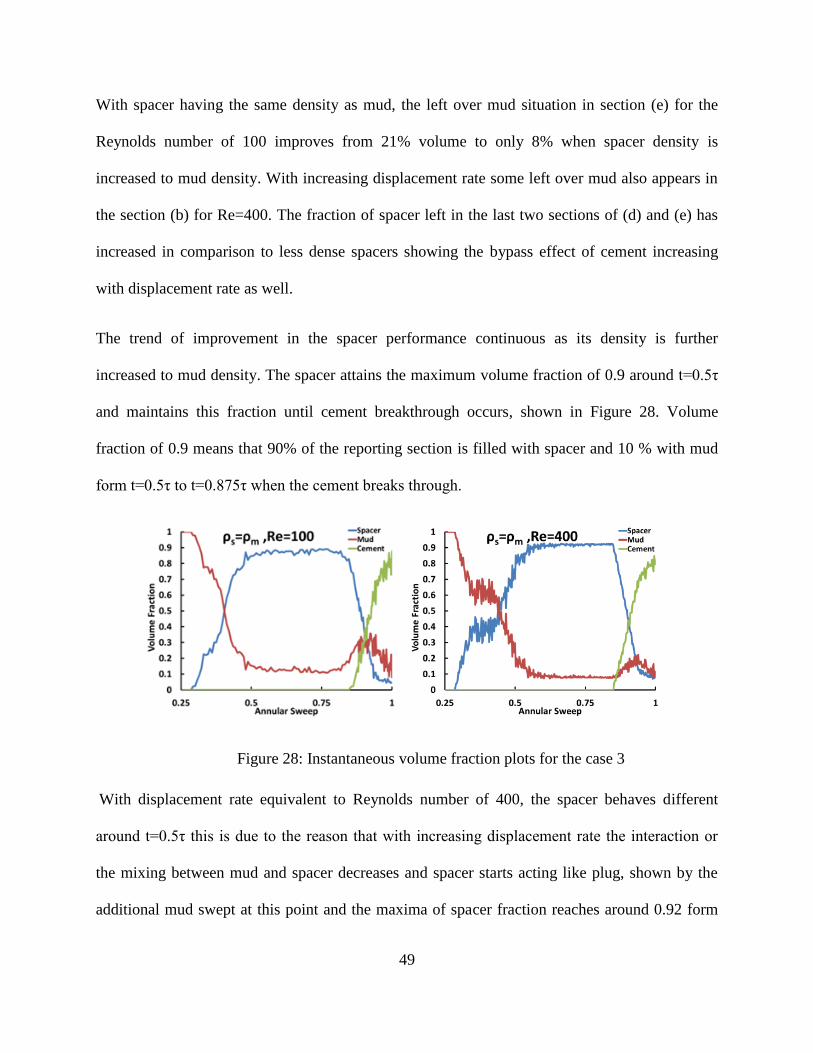
49

With spacer having the same density as mud, the left over mud situation in section (e) for the

Reynolds number of 100 improves from 21% volume to only 8% when spacer density is

increased to mud density. With increasing displacement rate some left over mud also appears in

the section (b) for Re=400. The fraction of spacer left in the last two sections of (d) and (e) has

increased in comparison to less dense spacers showing the bypass effect of cement increasing

with displacement rate as well.

The trend of improvement in the spacer performance continuous as its density is further

increased to mud density. The spacer attains the maximum volume fraction of 0.9 around t=0.5τ

and maintains this fraction until cement breakthrough occurs, shown in Figure 28. Volume

fraction of 0.9 means that 90% of the reporting section is filled with spacer and 10 % with mud

form t=0.5τ to t=0.875τ when the cement breaks through.


With displacement rate equivalent to Reynolds number of 400, the spacer behaves different

around t=0.5τ this is due to the reason that with increasing displacement rate the interaction or

the mixing between mud and spacer decreases and spacer starts acting like plug, shown by the

additional mud swept at this point and the maxima of spacer fraction reaches around 0.92 form

50

0.88 at Reynolds number of 100 and this additional mud sweep due to increased displacement

rate is also evident when cement breakthrough occurs in the form of lowest cement fraction peak.

Case 4: Similar trends for the left over volume fraction are observed as in the previous cases.

The left over volume fraction in section (c) increases with Reynolds number, the mud left in the

lower sections is more problematic as compared to the final section (e) where someone can argue

that we can flow some more than exact one annular flow. The cement fraction in the above three

sections of c, d and e decreases with increasing Reynolds number owing to the fact that now the

cement is bypassing some the spacer and correspondingly spacer fraction increase in these

sections.


51

The cement fraction in the above three sections of c, d and e decreases with increasing Reynolds

number owing to the fact that now the cement is bypassing some the spacer instead of giving it a

push type motion and correspondingly spacer fraction increase in these sections.

Interms of instabilities the trends continue to be the same as for the other lower densities. The

effect of increasing the displacement rate is similar to the cases with lower densities. The major

difference by increasing densty greater the mud is in the fraction of cement after one annular

sweep, shown in Figure 30. In the lower density cases it was above 0.8 after one annular sweep

but in this case it decrease and becomes worse with increased displacement rate. The reason is

that now the spacer becomes heavier than mud and due to push by cement that is even heavier

than spacer, these fluids pebetrates through the mud and mor spacer is left in the annulus after

one sweep. The phenomenon is clealy shown in volume fraction contour plots.


Spacer having less density in comparison to cement and being a Newtonian fluid leaves the

annulus quickly due to buoyancy affects, but when its density becomes greater than mud then its

left over fraction becomes severe in the case of spacer having density of cement.

52

Case 5: The problem of left over mud becomes severe as the spacer density is increased to the

cement density. A large fraction of left over mud can be seen starting from the lowest section b

up to the top section e, shown in Figure 31. As mentioned earlier the mud left in the lower

sections is difficult to remove.


While in contrast to lower density spacer cases, for this particular density of spacer the left over

mud fraction decreases with increasing Reynolds number, this can be observed in each individual

section. The pattern of mud left is shown in Figure 32. It can be observed that the mud left in this

53

case has a continuous layer alongside both the wall, and this layer is covered by a thick layer of

spacer.

a) b) c) d) e)

Figure 32: Instantaneous fluid fractions in sections (a, b, c, d and e) for case 5 after one sweep

As the spacer density becomes equal to cement, the fraction of left over spacer increases to such

a point that the spacer losses its effectiveness see Figure 33. Although the left over spacer

fraction decreases with increasing displacement rate, still it is too high to work with, therefore

the spacer with density equal to cement should be avoided and best results in terms of overall

spacer performance were obtained with spacer having the density equal to mud.


Mud

Cement

Spacer

54

The effectiveness of spacer can be measured in terms of the annular region it is present.

Figure 34: Spacer volume fraction in the observation section just before cement breaks through

in the observation sections for all of the cases 1,2,3,4 and 5

For ideal cases it should be 1 when it is completely displacing mud. If analyzed spacer fraction

just before cement breakthrough Figure 34, it can be observed that lighter spacer covers less

annular region as compared to heavier spacer. For spacer having cement density there is

apparently no effect or Reynolds number.

While looking at the overall cement fraction after one annular sweep in Figure 35, it is noticed

that the cement volume fraction for the lower Reynolds number the fraction is not affected by

increasing the density of spacer till the spacer density becomes equal to cement and at this point

the cement fraction decreases from 0.94 to 0.77, as mentioned earlier this decrease is the result of

Re

55

heavier spacer that is left in the annulus even when cement reaches at the exit. As the Reynolds

number is increased there is slight decrease in cement volume fraction with increase of spacer

density till spacer density becomes equal to cement density. While the trend for heaviest spacer

is opposite to the trends with lower densities. For densities less than cement, the cement fraction

decrease with increase of Reynolds number, while for the spacer with cement density the fraction

of cement has increasing trend.

Figure 35: Cement volume fraction at different Reynolds numbers and densities

6.2 Results for Spacer Viscosity and Displacement Rate Variations

Parametric study of varying spacer viscosity is performed while keeping the spacer density value

equal to average of mud and cement densities and varying the spacer viscosity from fresh water

viscosity to the cement viscosity. The spacer was taken as Non-Newtonian Power Law fluid.

Case 6 is covered in the previous section; it is same as case 4.

56

Case 7: The fraction of left over mud increases with increasing viscosity in all of the sections for

all the Reynolds numbers studied. The cement volume fraction has a slight decreasing trend with

increase of Reynolds number. The situation in terms of left over mud fraction becomes severe in

this case shown by the mud contamination indicator starting form section (b). In the last section e

the spacer left over volume fraction is nearly 0.2 in all of the Reynolds number. The spacer in

this case seems to be penetrated by cement from very start at the section a, where it is nearly 7%

of the total fluid in that section for all the displacement rates.


From the patterns of different fluid in this case it can be observed from Figure 37 that the spacer

is left from the very beginning of the section a and we move upward with different section the

57

spacer is covering a layer of left over mud along both the walls and in this case removal of mud

from walls will become cumbersome as we have to remove the spacer as well. So spacer

alongside with removal mud is creating problem by itself.

a) b) c) d) e)

Figure 37: Volume fraction contour of fluids after one complete annular sweep

In terms of stability of different interfaces and performance of spacer it can be seen that for

Re=100, as the spacer viscosity is increased from fresh water viscosity to the average of water

and mud viscosity, the instantaneous volume fraction of the spacer first increases and then

decreases indicating that there is significant mixing of mud and spacer behind the piston like

displacement of mud. The mixing of mud with spacer results in the local peak of the mud volume

Mud

Cement

Spacer

58

fraction. Similar trends are observed for higher displacement rates (Re = 167 and 400). However,

at high Reynolds numbers, the local peak in mud volume fraction is less prominent.

As mentioned earlier, when the spacer viscosity is in between fresh water and mud, the

displacement process is least effective and the cement volume fraction decreases and

substantially large volumes of spacer is left behind, but the process improves as the spacer

viscosity is further increased.


Case 8: With increasing the spacer viscosity to mud an overall positive effect can be observed in

nearly all of the section in terms of final cement fraction, the effect is prominent in the last two

sections where final cement fraction have improved more than 7% in comparison to the case 7.

An overall slight reduction in the mud volume fraction can also be observed in nearly all of the

sections in comparison to the spacer properties in case 7, but the decrease in mud fraction is not

very prominent.

59

Figure 39: Left over mud fractions in different sections for the case 8

The spacer performance in terms of keeping mud and cement separated has improved.


60

Now its plateau region is around 0.8 while in the previous cases it was around 0.75, which in

turn implies better separation agent. With increasing the Reynolds this plateau region shifts a

little bit downward and can be seen in Figure 40, there is no rapid mixing phenomenon observed

as it was with fresh water spacer.

Case 9: With further increasing the viscosity there is very minute changes in the left over mud

fraction in each section, but cement fraction has improved a little bit in each section as compared

to previous case, this indicates that in this case the spacer that is bypassed by cement has lesser

fraction in each section.


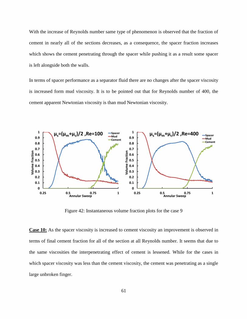
61

With the increase of Reynolds number same type of phenomenon is observed that the fraction of

cement in nearly all of the sections decreases, as a consequence, the spacer fraction increases

which shows the cement penetrating through the spacer while pushing it as a result some spacer

is left alongside both the walls.

In terms of spacer performance as a separator fluid there are no changes after the spacer viscosity

is increased form mud viscosity. It is to be pointed out that for Reynolds number of 400, the

cement apparent Newtonian viscosity is than mud Newtonian viscosity.


Case 10: As the spacer viscosity is increased to cement viscosity an improvement is observed in

terms of final cement fraction for all of the section at all Reynolds number. It seems that due to

the same viscosities the interpenetrating effect of cement is lessened. While for the cases in

which spacer viscosity was less than the cement viscosity, the cement was penetrating as a single

large unbroken finger.

62


With increasing spacer viscosity its Reynolds number decreases and gradually its flow regime

turns to Laminar when its viscosity reaches the mud viscosity. Due to its higher viscosity instead

of creating the rapid mixing the spacer now starts penetrating the less viscous mud and therefor a

continuous layer of mud can be observed for all of the cases with spacers having higher

viscosities than fresh water. The spacer is present along both the walls from the very begging of

first section (a). The mud removal in this case will be very difficult as now if we closely observe

in the top four sections of (b, c, d and e), a buffer layer of viscous spacer is covering a

continuous mud layer adhered to walls.

63

a) b) c) d) e)

Figure 44: Volume fraction of fluids after one complete annular sweep for case 10

There are no apparent changes in the behavior of overall system, except that the cement

breakthrough in the section e is delayed a little bit.

Figure 45: Instantaneous volume fraction plots for the case 10 increasing displacement rate

For all the displacement rates it has been observed that the rate of mud removal (i.e. the slope of

mud volume fraction) is prominent for the less viscous spacer especially having the viscosity of

Mud

Cement

Spacer

64

water. In this case a fraction of 0.10 is obtained in the channel around half of annular flow. The

amount of mud that is swept by cement decreases for high viscosity spacers.

The trends for the cement fraction in the entire annular section are similar to the last 10 ft

section. Fraction slightly decreases with increasing Reynolds number and the minimum values

fraction are observed when spacer viscosity becomes equal to mud viscosity shown in Figure 46.

However the trend of decrease in fraction with viscosity is reversed when spacer viscosity is

further increased towards cement at all Reynolds numbers. Then the cement fraction increases

with viscosity.

Figure 46: Cement volume fraction at different Reynolds numbers and viscosities

65

6.3 CFD Based Correlation

Due to the nature of fluid being used the correlation for the 50 ft of annulus is expected to be of

the form of power law

φ

Where φc is the cement volume fraction, is a constant multiplier,

√

√

Re is the Reynolds number and a, b, c are constants.

For vertical wells to correlate the performance of spacer based on its density, viscosity and

displacement rate, the plots of volume fraction of cement after one annular flow are plotted

against varying spacer densities and viscosities. The results indicate wide deviation in cement

volume fraction when spacer density becomes equal to cement as shown in Figure 47. The

strange behavior on the apparent viscosity plot is attributed to the shift in the apparent viscosities

of cement and mud with increasing Reynolds number, sees section 5.2 for details.

Figure 47: Cement volume fraction after one annular flow over the entire length

66

To obtain the correlation data of three cases were exclude to see whether the data for these cases

could be generated by the correlation without using the CFD simulations.

Table 5, shows the values of different constants obtained from the straight line fits

(see appendix –A) for details

Table 5: Constants Obtained From Plots

Variable a b c 1 2 3

Value -0.1011 -0.0167 -0.0169 0.90413 0.74322 0.95199

The resultant form of the correlation is given below in Eq. 2, 3 and 4

(

)

Data to check the goodness of fit in the form of R2 value is given in

Table 6, on next page. The procedure to find R2 is described in appendix-A. R

2 value of 1 will

show an exact fit and lesser value will show deviation form exact fit. The value of R2

was found

to be 0.774, which is not a perfect fit.

67

Table 6: CFD and Correlation Data Comparison and Calculation of R2

Value

ρ μ Re CFD (a)

Correlation (b)

(a-b)2 (a-aavg)2

0.58 0.00 100 0.94 0.97 8.8E-04 2.7E-03

0.74 0.00 100 0.92 0.95 5.4E-04 1.1E-03

1.00 0.00 100 0.93 0.92 4.8E-05 1.3E-03

1.10 0.00 100 0.72 0.75 6.2E-04 2.7E-04

0.58 0.00 167 0.93 0.96 1.3E-03 1.4E-03

0.74 0.00 167 0.94 0.94 6.4E-06 2.1E-03

0.91 0.00 167 0.93 0.92 8.1E-05 1.5E-03

1.00 0.00 167 0.91 0.91 4.3E-06 5.3E-04

1.10 0.00 167 0.73 0.74 1.6E-04 1.2E-04

0.58 0.00 400 0.94 0.95 7.1E-05 2.6E-03

0.74 0.00 400 0.93 0.93 1.8E-05 1.5E-03

1.00 0.00 400 0.88 0.90 2.9E-04 8.9E-05

1.10 0.00 400 0.77 0.73 1.3E-03 7.5E-04

1.00 0.00 100 0.93 0.92 4.8E-05 1.3E-03

1.00 0.47 100 0.82 0.85 5.4E-04 4.5E-03

1.00 0.80 100 0.84 0.84 3.7E-07 2.6E-03

1.00 1.18 100 0.86 0.83 6.8E-04 9.4E-04

1.00 1.25 100 0.88 0.88 3.6E-06 2.4E-05

1.00 0.00 167 0.91 0.91 4.6E-06 5.3E-04

1.00 0.44 167 0.81 0.84 7.6E-04 6.1E-03

1.00 1.00 167 0.85 0.83 3.9E-04 1.7E-03

1.00 1.02 167 0.86 0.87 1.5E-04 9.7E-05

1.00 0.00 400 0.88 0.89 1.6E-04 8.9E-05

1.00 0.53 400 0.82 0.83 3.5E-06 4.5E-03

1.00 1.06 400 0.84 0.82 5.7E-04 2.6E-03

1.00 1.00 400 0.86 0.82 1.9E-03 9.4E-04

1.00 0.94 400 0.88 0.86 2.1E-04 2.4E-05

6.3.1 Example Calculation Using Correlation

Now we use the correlation to find the final cement volume fraction for the cases whose data

were not used to find the correlation and see how accurately values can be predicted with

correlation. For the case of Re= 100 and when spacer has density of mud and viscosity of water,

we have

68

√

√

Percentage difference

φ φ

φ

Similarly for other values whose CFD data was present, the comparison between the CFD values

and correlation values is shown below in

Table 7.

Table 7: Comparison of CFD and Correlation Values for Final Cement Volume Fraction

ρ μ Re CFD Correlation % Difference

0.911 0.003 400 0.920 0.907 1.44

0.579 0.003 167 0.937 0.958 -0.07

It can be observed that the correlation can be used to obtain the values for some of the other

spacer properties combinations whose simulations were not performed. Therefore it can be used

to optimize the displacement process for this particular combination of mud-cement properties.

The accuracy of the correlation for generic situations needs to be tested as the correlation is

based only on a single annular sweep data having one combination of mud-cement properties

only.

69

6.4 Results with Eccentricity and Displacement Rate Variation

In these set of simulations the eccentricity is varied from 0.05 to 0.95 for the vertical cases. The

hole and casing geometry and fluid properties are the same as were for the concentric vertical

cases.

Sectional view of full 3D grids having 105,000 hexahedral cells is shown in Figure 48.

Figure 48: Section view of concentric case with hexahedral cells

From the previous simulations it was found that the spacer with density of mud and viscosity of

water are more efficient as compared to other fluid combinations, so far this section the density

and viscosity were fixed to be that of mud and water respectively. Due to increase of

eccentricity, the yielding fluid behavior becomes very important, therefore in this series of

simulations the fluid rheologies of mud and cement were modeled with Herschel Bulkley

rheological model.

Case 11: For this very small eccentricity and at all Reynolds number studied so far, for the three

bottom sections a, b, c have perfect cement job i.e. 100 % cement, no mud or spacer in these

70

sections. The second last section (d) for all the Reynolds numbers have some mud fraction in that

section which increases with Reynolds number and spacer fraction in this section is zero. The

last section e has a lot of mud present which has increasing tendency with Reynolds number and

some spacer fraction is also present which also has increasing tendency (0.11 to 0.20) with

Reynolds number.


The temporal variations in volume fractions of different fluid in section (e) are shown below in

Figure 50. As pointed earlier it can be observed that with the increase of Reynolds number for

the same eccentricity the cement fractions decreases. The curve of cement fraction for the higher

71

displacement rate has a continuously increasing trend while at lower displacement rate some

fluctuations can be seen.

Figure 50: Instantaneous fluid volume fraction in different sections for the case 11

Case 12: With the increase of eccentricity the mud fraction left in section d increase in

comparison to e=0.05. The left over mud has an increasing tendency with Reynolds number. The

lower three sections in this case also has perfect cement job. The top section (e) has a large

fraction of bypassed mud along with some fraction of spacer. The decrease in cement fraction in

the section (e) with increasing displacement rate can be explained by similar arguments as for the

concentric vertical cases that depending on the displacement rate the interfaces of cement-spacer

and spacer-mud behave differently. Both Rayleigh-Taylor and Saffman-Taylor instabilities grow

and some of the spacer is also left behind, while below a certain critical displacement rate the

instabilities does not grow rapidly and the sweep is good.

72


The left over mud patterns for Reynolds number of 100 and 400 are shown in Figure 52. The

increase in the left over mud and spacer fraction is clearly visible. One major observation that

can be made is that for the Reynolds number of 400, the spacer presence can be seen in the

narrow side of the annulus, while for the lower Reynolds number case only the mud is present in

the section (e). It implies that for some eccentric cases in which the eccentricity is not very

severe, the mud displacement efficiency can be enhanced by increasing displacement arte

73

Section d) d) e) e)

Re 100 400 100 400

Figure 52: Left over mud pattern comparison for e = 0.25 on a plane showing the wider and

narrow gaps and at four radial planes

In terms of interfacial stability, same trend of e =0.05 is followed in this case, only difference is

in the increase of mud volume fraction during the sweeping process shown by the flat plateau

region in the graph, shown in Figure 53. The spacer left over after one annular sweep increases

with displacement rate but increase is not as significant as was in the case of low eccentric case

of 0.05. The spacer maximum fraction reached in this case is around 0.8 which is less then as

compared 0.85 with eccentricity of 0.05, this is due to the reason that more mud is present in the

observation section at all times during the sweep.

74


Case 13: The left over mud fraction for e =0.5 is shown in Figure 54 below.


75

It can be observed that with further increase in eccentricity the left over mud in the last two

sections (d) and (e) increases in comparison to lower eccentric cases and in this case left over

mud start appearing the section (c) also. The increase in left over mud fraction in the last section

is not very prominent while for the section (d) it increase from 0.07 to 0.15 of the total volume of

fluid in that section.

With increase of eccentricity for all displacement velocities the fraction of cement in the

observation section has increased in comparison to low eccentric cases Figure 55. The plateau

region of mu volume fraction remains around 0.28 at all times during the whole annular sweep.

This is 0.08 high as compared to the case with eccentricity of 0.25. The reduction of spacer

fraction after one complete sweep and high volume fraction of mud in this section shows that

mud is trapped and spacer flows in the wider sider of the annulus and is not sweeping mud as it

should be.


Case 14: With the further increase of eccentricity the mud starts appearing in the bottom section

b as well, while for middle section (c) it has now increased to the approximately 10% of the total

fluid volume in that section. One thing to be noted that in nearly all of the sections the spacer left

76

behind is nearly zero for Re of 100 and 167, while for Re=400, nominal fraction of spacer is

present in the last two sections only. When compared to lower eccentric cases this suggests that

due to constriction that the spacer finds on the narrow side of the annulus it takes the path of

wider side and leaves the channel, means it is now mainly flowing on the wider side of the

annulus and it is not sweeping the static mud on the narrow side.


In these cases the eccentricity has increased to such a point that the fraction of mud never

decrease below 0.32 at any time during the displacement process. As the narrow side becomes

smaller and smaller the spacer and cement prefer to move along wider side and consequently the

spacer fraction after one annular sweep is near zero for e = 0.75 shown in Figure 57.

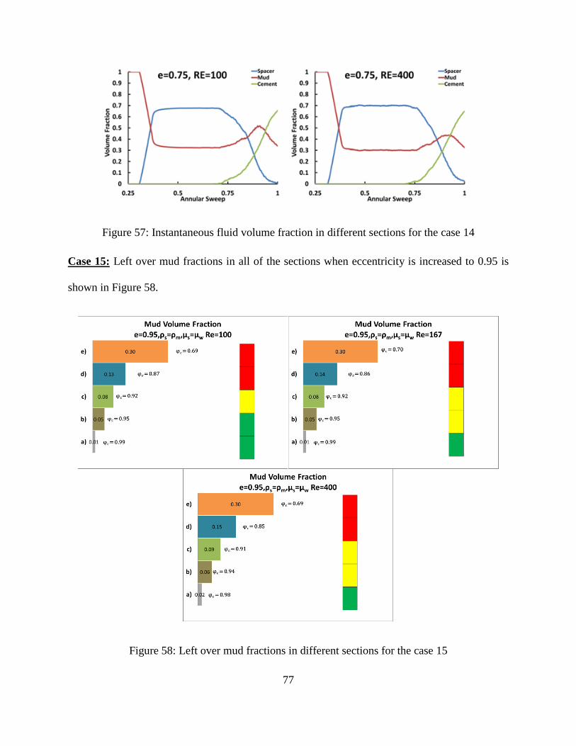
77


Case 15: Left over mud fractions in all of the sections when eccentricity is increased to 0.95 is

shown in Figure 58.


78

As the eccentricity increased from 0.75 to 0.95 it can be observed form, in the last three sections

the fraction of left over mud decreases. The reason for this decrease is the very narrow gap. This

fraction is the area weighted average and now the ration of wider to narrow is very large, so most

of the flow takes the path of wider side and the mud that is static is confined in the less area due

to very narrow gap. The main difference from the previous cases with lower eccentricity is the

small amount of left over mud in lowest two sections as well.

The severity of left over mud on the narrow side of the annulus can be seen in Figure 59. The

mud form narrow side is barely moved at all. The continuous layer of mud starting from very

first section goes till the end of annulus.

a) b) c) d) e)

Figure 59: Fluid volume fraction in different section for the case 15

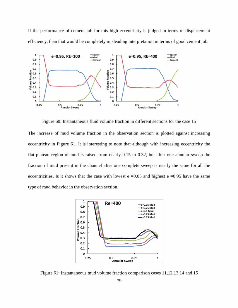
79

If the performance of cement job for this high eccentricity is judged in terms of displacement

efficiency, than that would be completely misleading interpretation in terms of good cement job.


The increase of mud volume fraction in the observation section is plotted against increasing

eccentricity in Figure 61. It is interesting to note that although with increasing eccentricity the

flat plateau region of mud is raised from nearly 0.15 to 0.32, but after one annular sweep the

fraction of mud present in the channel after one complete sweep is nearly the same for all the

eccentricities. Is it shows that the case with lowest e =0.05 and highest e =0.95 have the same

type of mud behavior in the observation section.

Figure 61: Instantaneous mud volume fraction comparison cases 11,12,13,14 and 15

80

Case 16: It has been observed that a combination of lighter preflush followed by a heavier

spacer performs better in comparison to the heavier spacer alone. Various combination ratios of

heavier spacer having density, average of mud and cement and viscosity of fresh water with

lighter preflush water are studied. Comparison is shown in the Figure 62. It has been observed

that for a particular combination ratio of 5 ft preflush followed by 45 ft heavier spacer, the mud

displacement was significantly improved and cement fraction in the observation section was

increased from 0.72 to 0.79, i.e. 7% increase in cement volume fraction. Please note that this

cement fraction is only in the most critical portion of annulus i.e. in the last 10 ft section, while

overall fractions in the entire annulus will be different from this.

Figure 62: Fluid volume fractions in the reporting section after one annular flow for lighter

preflush followed by heavier spacer

81

7. HORIZONTAL WELL WITH VARIABLE ECCENTRICITY

7.1 Introduction

Extended reach wells can offer significant commercial advantages. Greater drainage coverage of

a reservoir is achievable from fewer locations. Therefore there has been increased focus on

horizontal and deviated well development due to their two major applications in enhanced oil

recovery and unconventional hydrocarbon prospects. Factors contributing to the overall

performance of a horizontal completions are similar to vertical completions, but have additional

contributions from the, solid particle settlings on lower side of annulus and free water channels

on the upper side of the annulus and hole eccentricity.

Deposition of solids in the wellbore is one of the most severe problems in horizontal wells

(Keller et al. 1987). Settling of barite or drill cuttings causes the mud on the low side of

the annulus to have a higher density than the mud on the top side. The amount of solids, or

channel size, appears to be a function of the rate of deposition and the rate of particle erosion by

hydrodynamic forces. Even though smaller particles may remain in suspension, larger

particles may not, and in horizontal systems they accumulate in the narrowest part of the

annulus, which further diminishes the capability of the mud to remove them from the well. Mud

and settled drill solids which are not properly removed from the wellbore with the drill string can

be a hindrance in getting casing to bottom in horizontal wells and these settled solids will be

much more difficult to remove once casing is placed into the well. The best approach to

minimize the settling problem is a properly designed mud system which is able to

adequately transport solids and drill cuttings from the well.

82

Solids settling are not limited to the drilling mud, but also occur in the cement slurries if proper

precautions are not observed. Proper slurry design is of utmost importance not only to prevent

particle settling, but also to help insure appropriate rheologies for efficient placement and

mud removal, as well as providing zero free water to help provide top-side integrity in the

annulus.

Keller et al.(1987) conducted a series of lab experiments in which they simulated the solid

particle settling in a concentric annulus at various wellbore orientations. They showed that even

with concentric annulus there was a huge difference in the displacement efficiency, between the

top and bottom section of the annulus at different orientations. The problem was aggravated for

certain combination of fluid properties and flow rates.

Cement slurries that have free water and/or settling tendencies can result in water channels on

the top side of a horizontal annulus, or an area of reduced compressive strength cement which

may not provide the annular seal required for zonal isolation during stimulation treatments. It is

very important that zero free water slurries be used in horizontal cementing applications.

Figure 63: Depiction of typical horizontal well cross section

83

In horizontal well, there has been an increased possibility of having narrow annular channel on

lower side and wider channel on other side of the casing. Insufficient clearance on the narrow

side of the wellbore can result in portions of the well that are not cemented properly or even not

cemented. It is due to the fact that due to narrow path excessive viscous forces have to be

overcome to mobilize the mud or solid settled cuttings on narrow side while due to lower

resistance on the wider side of the annulus fluid has the tendency to follow the path of less

resistant and move in the wide in the wider side. The problem could be so severe that tops of the

cement on the two side of the annulus can be separated by hundreds of feet (Sabin, 1990). So

any casing eccentricity further complicates the horizontal cementing process.

The severity of these factors can be reduced by the design of a good displacement process and

special slurries for horizontal wells.

There are four possible techniques to complete horizontal wells

Open hole

Slotted or perforated liner

Slotted liner with external casing packers

Cementing casing or liner

First three are called “drainhole” completions and fourth one is usually called “cased hole”

completion. Cementing of a horizontal well is recommended when there exits the water bearing

zones in the vicinity that may be connected by natural fractures of faults. Lack of natural barrier

may also force the cementing of horizontal wells. Cementing of horizontal well is also important

when cement sheath have to work as a conductor of heat which can conduct heat from formation

84

fluids and deliver it to casing; this is the case of geothermal wells. Cement is necessary in this

case as the formation is a poor conductor.

Problems encountered during horizontal well cementing are similar to those of vertical well

cement job, but are worsen by factors such as wellbore orientation, geometry, gravitational

forces and in the case of shale gas containment of fracture pressure within treating interval as

related to fracture volume size, and number of stages to be performed. Past investigators have

identified a number of critical factors that are important to have successful primary cementing in

vertical wells, including mud conditioning, pipe movement, high cement flow rates, pipe

centralization and the use of spacers or preflushes. Most of these parameters are also important in

deviated or horizontal wells.

There are a number of techniques that can be effectively applied for primary cementing, there

application are more cumbersome in horizontal wells as compared to vertical wells. For example

it is more difficult to achieve pipe centralization in a deviated well due to the weight load of the

casing acting to bend the casing towards the lower side of the annulus. This will not only create

high resistance to flow on the narrow side of the annulus but also can produce torque and

bending stresses that can lead to restrict the pipe movement. If the inner pipe of the annulus is

not centered, the velocity distribution around the annulus is distorted, the flow favoring the wider

side. This may lead to unusual situations where the flow regime can be laminar on the narrow

side of the annulus and turbulent on the wide side, because the local Reynolds number varies

azimuthally around the annulus (Nelson, 2006). Pipe centralization significantly aids in mud

displacement.

85

A successful cementing operation relies on a cementing system that provides casing

support and isolation from unwanted zones. To obtain this, all of the preceding best

practices should be considered. The final cementing design should have all the

characteristics necessary to complement these best cementing practices. Conventional

cement slurries or non-nitrified cement have been the basis for designs for many years.

Low-density slurries have ranged from water, extended with emphasis on low cost, to

specialized hollow microsphere formulations to provide better compressive strength

development. In some areas, acid soluble systems have been used as well.

7.2 Problem Setup

The casing was assumed to be supported by two centralizers at both ends and has uniformly

distributed load on it.

Figure 64: Beam supported on its ends with uniform force distribution

The equations describing the bending of the casing at any point and maximum bending along x-

axis is given below

Where E is modulus of elasticity of material, w is weight/length and I is the moment of inertia.

From literature review it was found that most of the horizontal wells were completed with 8.5" of

w

x

86

open hole with either 7.5" or 5.5" casing. In this set of simulations 5.5" casing was used. The

casing date is given in Table 8 below.

Table 8: Casing Data

The spacing between the centralizers was varied to achieve maximum eccentricities of 0.15, 0.3

and 0.6 at center. Casing section length, maximum deflection at center and eccentricity is given

in Table 10.

Assuming that the same fluid is present inside and in the annular region of casing, the buoyancy

factor is given by

(

)

Substituting the values of mud and cement densities, the buoyancy factor in this case has value

of 0.838. The buoyancy effects with different fluids inside and outside the casing. Let’s look at

the worst possible scenario in terms of casing deflection i.e. when the cement is inside the casing

and preflush water is in the annulus, the buoyancy factor proposed by (Lee et al., 1986) is given

by

(

) (

) (

)

(

)

C-95 23 Dh in Do(Cas)in Di(Cas)in E(Mod)psi I(Mom)in^4

NW

(lbm/ft)

Clearance

(in)

P-110 8.500 5.500 4.670 2.900E+07 21.571 23.000 1.500

87

Where and are the preflush and cement density respectively. Using this expression the

buoyancy factor is found to be 0.796; the maximum deflections and eccentricity for this case are

shown in Table 9.

Table 9: Casing Deflection and Corresponding Eccentricity

Section

Length (ft)

Air inside and outside

casing

Mud inside and in the

annulus

Cement inside and water

in the annulus

Max def

(in) Eccentricity

Max def

(in) Eccentricity

Max def

(in) Eccentricity

48.29 0.90 60.00 0.84 56.28 0.72 47.76

40.61 0.45 30.00 0.42 28.14 0.36 23.88

34.15 0.23 15.00 0.21 14.07 0.18 11.94

The most severe case occurs for the weight only in air and in this simulation this case was

considered. As three cases were considered for this analysis, so for casing with buoyed weight,

the cases with lesser maximum deflections can be inferred.

The fluid data used is a case history taken from Schlumberger Horizontal Well Cementing

(2005), shown in Table 10.

Table 10: Fluids Data from a Case History - Malaysia

Fluid 1 ρ(lb/gal) μp (cP) τy

(lb/100ft2)

n K (eq. cP) μa(cP)

Mud 10.2 34 13 0.7848 179.51 77

Cement 15.8 34 4 0.92146 61.8936 49

Pump rate: 10 bbl/min which corresponds to Reeqcr = 1309, Reeq = 3304. So the flow is turbulent

and in these cases k-ϵ turbulent model was used with standard wall function and default setting

in the CFD code. For each case the computational domain is divided into three equal sections,

described below for the flow analysis and left over mud quantification.

88

Figure 65: Sections for leftover mud analysis

7.3 Cases Studied

Four cases corresponding to each eccentric value of 0.15, 0.3 and 0.6 were considered with

Newtonian spacer having the following properties with fluid dataset from Table 10.

Table 11: Spacer Density and Viscosity Variation

Case

#

Max.

Eccentricity at

Centre

Spacer Density

ρs (lbm/gal)=

Spacer Apparent

Viscosity μs (Cp)= Reynolds #

1 0.15,0.3,0.6 ρm =10.2 μm =78 3304

2 0.15,0.3,0.6 ρm =10.2 μc =49 3304

3 0.15,0.3,0.6 ρc=15.8 μm =78 3304

4 0.15,0.3,0.6 ρc=15.8 μc =49 3304

Eccentricity = 0.15: Grid consisted of 80000 hexahedral cells with fulfilling the near wall grid

requirements for the k-ϵ turbulence model with standard wall functions; geometry is shown in

Figure 66.

Figure 66: Geometric of e = 0.15

The left over mud fraction in the three sections described in Figure 65 for all of the four cases for

e=0.15 are shown Figure 67. For all of the cases the mud left in the last section is largest in

34.15ˊ

Section 1 Section 2 Section 3

Inlet Outle

89

comparison to the other sections. The decrease of spacer viscosity from mud viscosity to cement,

there is no change in the cement fraction in all of the sections, but a very minute change in the

mud fraction i.e. a slight increase was observed. As the spacer density is increased to cement in

case 3, the mud fraction is significantly decreased from 10 to 5 % in the section 3 towards the

exit, but with a penalty of 20% spacer leftover as well. The reduction in mud fraction can be

attributed to the positive density differential between mud and cement.

Figure 67: Leftover mud fraction for the cases 1, 2, 3 and 4 with e=0.15, Re=3304

While looking at the plots it can be seen for spacer and mud the change of spacer viscosity does

not plays a prominent role in in the displacement process while changing the spacer density

offset the results apart. The small or no change due to spacer viscosity variation could be

(Case 1) (Case 2)

(Case 4) (Case 3)

90

attributed to the fact that for this particular case viscosities of cement and mud do not differ

widely. While there is significant difference between mud and cement densities and when spacer

density is varied the results are offset. While looking at the cement behavior it seems that for

annular sweeps up to 0.8, it is not affected by the variation of spacer density or viscosity either.


with e=0.15, Re=3304

While slight variation exits when the spacer is approaches exit. As we have seen in vertical well

cases that when spacer density approaches cement then the amount of spacer left in the annulus

increases, same phenomenon is seen in this case. While looking at the spacer volume fraction

plot it becomes clear that for higher densities the fraction of spacer left in annulus even after one

annular sweep is large, while the mud fraction after one sweep does not differ widely.

Moreover these are overall volume fractions of fluids and these are not good representation of

the severity of the problem. Taking the overall values and averaging them on the volume will

hide some the critical portions of the annulus. For example there may be a significant amount of

mud trapped in some localized area occupying 20-30% of annular cross section at that [particular

91

point and when we look at the overall volume fractions i.e. averaged over the entire volume this

type of severities are averaged out and hidden. So looking at the overall mud sweep efficiency is

not a good indicator of the potential critical areas where mud channels can exit. The contours of

volume fraction of different fluids after one annular sweep are shown in Figure 69. For the cases

when spacer density is equal to mud i.e. case 1 & 2, the spacer left in the annulus is clearly

visible towards the last section of the annulus.

Figure 69: Fluid volume fraction contour on an axial and three radial planes towards the exit

The mud left in all of the cases is toward the wide side of the annulus, this is due to the reason

that the flow is sufficient enough to displace the mud form narrow side, but on the wider sider

the flow faces an expansion. This reduces pressure and the fluid moves towards the upper side

due to this pressure differential. For the case 1 and 2 clearly this is the reason while for the cases

3 & 4 gravity is also a contributing factor and some mud fraction may be riding on both spacer

and cement and in these cases spacer fraction also increases on the narrow side of the annulus.

The constriction that the flow finds on the narrow side is depicted in terms of stream line plots

Case 1

Case 4

2 ft 2 ft Exit

92

shown in Figure 70. Although with e =0.15 this phenomenon is not prominent but it will be

noticeable for larger eccentricities.

Figure 70: Streamline plot colored by mixture volume fraction after one complete sweep

Eccentricity = 0.30: Grid in this case consisted of 93000 hexahedral cells; geometry is shown in

Figure 71.

Figure 71: Geometry with e = 0.30

In terms of fluid volume fractions after one complete annular sweep, there are no major changes

observed when the variable eccentricity takes the maximum value of 0.3 at the center of the

casing.

40.61ˊ

Case 4

Case 1

Outlet Inlet

93


Similar trends for instantaneous volume fraction for all of the fluids can be found with

eccentricity of 0.3 shown in Figure 73. The major difference is in the interplay of the mud and

spacer fractions and deviation between different density fluids becomes larger with increasing

eccentricity. There is also the decrease in cement fraction at the end of one annular sweep. For

heavier spacers more spacer is left in the annulus as compared to eccentricity of 0.15. If we

closely look at the mud plot, then we can recognize that the fraction of the mud left in the

annulus after one annular sweep is nearly the same either for e=0.15 or e=0.3, only the fraction

of spacer left in the channel increases for spacers heavier than mud.

94


As the gap is becoming narrower the majority of the fluid tries to go through the wider side and

with the increase of spacer density case 3 and 4, the spacer left over even after one sweep has

increased in this case shown in contour plots of Figure 74.

Figure 74: Fluid volume fraction contour on an axial and three radial panes towards the exit

The effect of restriction to flow is becoming dominant depicted by the lift of stream line around

the center point of the casing where it has most deflection, shown in Figure 75.

Case 4

Case 1

2 ft 2 ft Exit

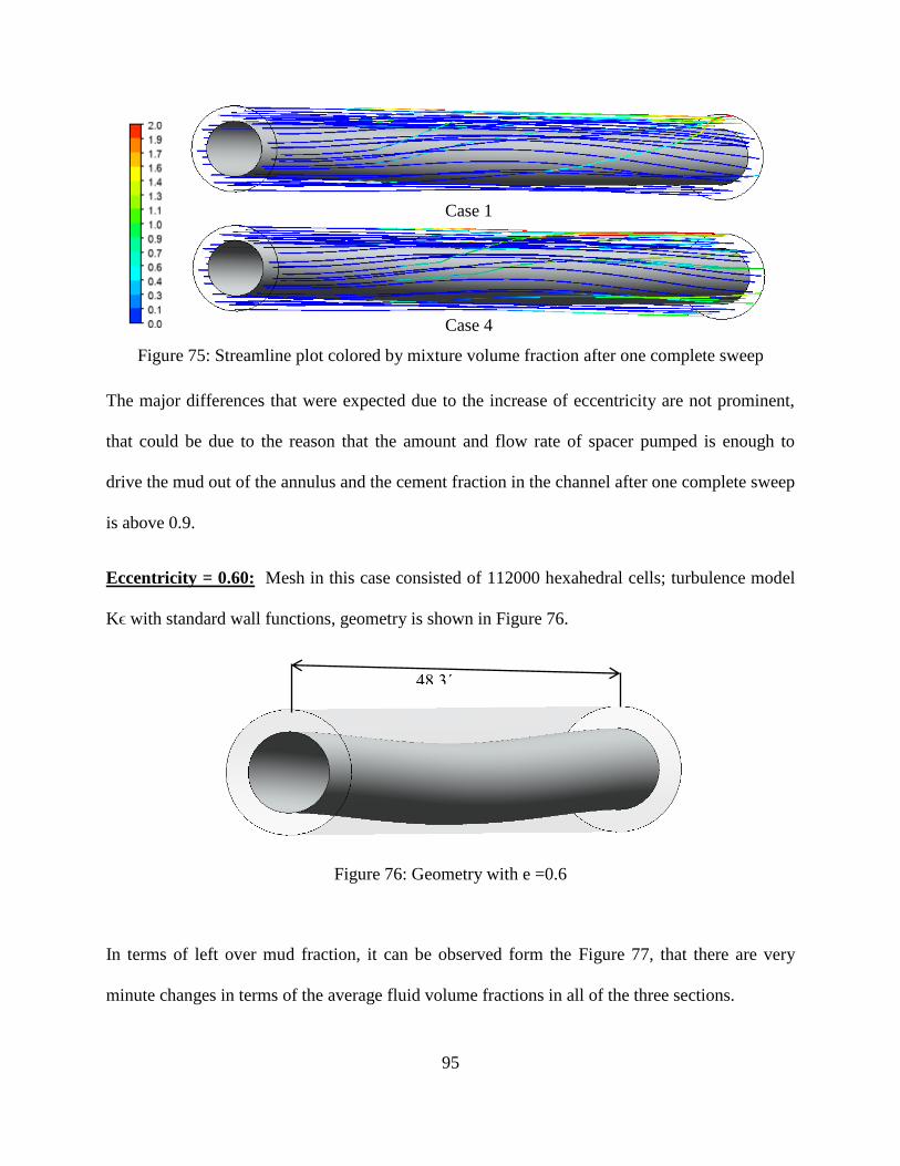
95

Figure 75: Streamline plot colored by mixture volume fraction after one complete sweep

The major differences that were expected due to the increase of eccentricity are not prominent,

that could be due to the reason that the amount and flow rate of spacer pumped is enough to

drive the mud out of the annulus and the cement fraction in the channel after one complete sweep

is above 0.9.

Eccentricity = 0.60: Mesh in this case consisted of 112000 hexahedral cells; turbulence model

Kϵ with standard wall functions, geometry is shown in Figure 76.

Figure 76: Geometry with e =0.6

In terms of left over mud fraction, it can be observed form the Figure 77, that there are very

minute changes in terms of the average fluid volume fractions in all of the three sections.

48.3ˊ

Case 1

Case 4

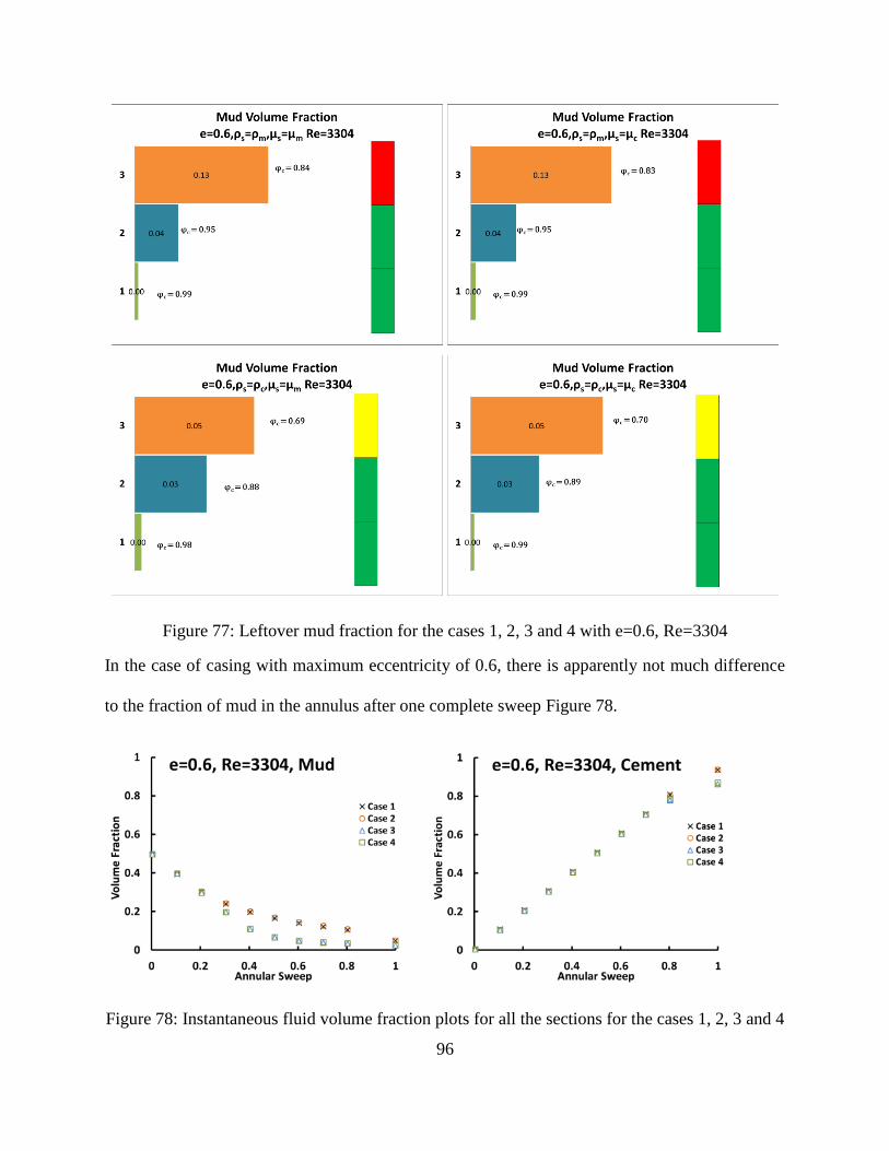
96


In the case of casing with maximum eccentricity of 0.6, there is apparently not much difference

to the fraction of mud in the annulus after one complete sweep Figure 78.


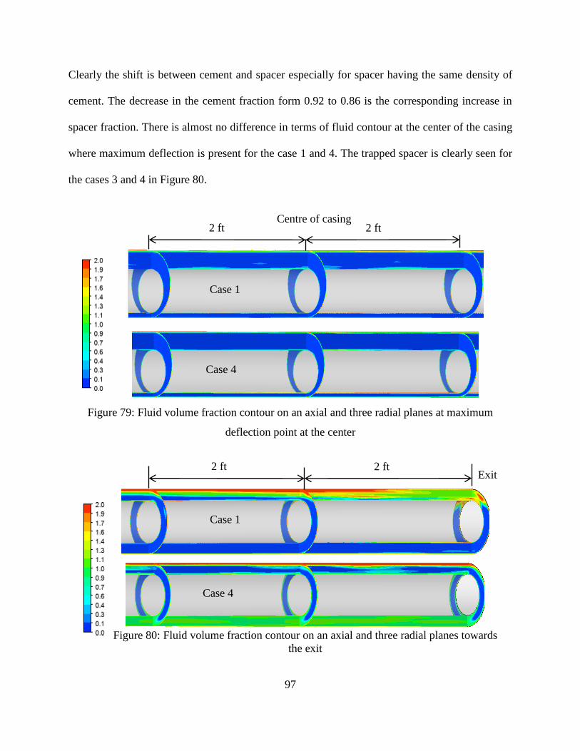
97

Clearly the shift is between cement and spacer especially for spacer having the same density of

cement. The decrease in the cement fraction form 0.92 to 0.86 is the corresponding increase in

spacer fraction. There is almost no difference in terms of fluid contour at the center of the casing

where maximum deflection is present for the case 1 and 4. The trapped spacer is clearly seen for

the cases 3 and 4 in Figure 80.

Figure 79: Fluid volume fraction contour on an axial and three radial planes at maximum

deflection point at the center

Figure 80: Fluid volume fraction contour on an axial and three radial planes towards

the exit

Case 4

Case 1

Case 1

Case 4

2 ft 2 ft Exit

2 ft 2 ft Centre of casing

98

It can be seen that the cement in this case even after one annular sweep has only reached to the

center point and rest of the leading section on the narrow side of the annulus is filled with spacer.

The Newtonian nature of spacer have helped it in getting through narrow constriction, while if it

were to be non-Newtonian fluid the flow physics would be very different in that case.

The resistance to the flow in passing through the narrow gap is the maximum in this case, shown

by the more curved stream line contours Figure 81. Some of the fluid prefers to travel on the

wider side shown by the crossing stream line. As the stream lines are colored by mixture volume

fraction, so the place and fraction of each fluid can be seen at all points along the entire annulus.

Figure 81: Streamline plot colored by mixture volume fraction over entire domain

7.4 Laminar Vs. Turbulent Flow Number Comparison

To see the effect of increasing the displacement rate on the mud displacement and final cement

fraction two displacement rates corresponding to Re = 700 & 6377 were used. The spacer has the

same density and viscosity as mud but it is Newtonian fluid. It can be seen form Figure 82 that

the fraction of cement is not badly affected by the increase of displacement rate. For the lower

Case 1

Case 4

99

displacement rate the fraction of mud left in the annulus is nearly double in comparison to

fraction at higher displacement, while some spacer is also left with increase of displacement rate.

Figure 82: Instantaneous volume fraction plot for e = 0.6 for laminar and turbulent flows

The complete removal of spacer at low Reynolds number and some fraction of mud left can be

attributed toward the Newtonian and Non-Newtonian nature of theses fluids. Mud being having a

certain yield stress will be mobile when this stress have been overcomed, but at lower

displacement rate this does not seem to be the case.

7.5 Same Flow Rate Different Fluids

The data for comparison was taken from another case history data. The fluid properties are given

in Table 12.

Table 12: Fluid 2 Rheological Data

Fluid 2 ρ(lb/gal) μp (cP) τy

(lb/100ft2)

n K (eq. cP) μa(cP)

Mud 11.3 16 12 0.6517 245.28 52.2352

Cement 16 28 8 0.8296 104 55.79

In the result analysis Fluid 1 represents the fluid data form case history of Malaysia (Table 10)

and Fluid 2 represents the data from case history Denmark (Table 12). To see the effect of

100

changing the fluids involved on the overall performance of the system, the results of two

simulations are compared in Figure 83. In both the cases the spacer was having the density and

viscosity of mud but was a Newtonian fluid. Details of fluid 1 and 2 are provided in tables 9 and

10 respectively. Fluid 1 is more promising as for this case at the end of one sweep the fraction of

cement is maximum. There major contributing factor for better performance of fluid 2 seems to

be the very small difference in the mud and cement viscosities.

Figure 83: Instantaneous volume fraction plot for e = 0.6 for fluid 1 & 2

101

8. SUMMARY AND CONCLUSIONS

A detailed computational fluid dynamics study is performed to investigate the effect of spacer

fluid properties on the effectiveness of mud displacement during the cement placement process.

Simulations model the non-Newtonian fluids as Power-Law/ Herschel Bulkley fluids and track

various fluid volume fractions in time-resolved fashion in the three-dimensional annular space. A

validation study for both concentric and eccentric cases shows good agreement between

simulation and experimental results of Tehrani et al. (1992). Over 60 parametric simulations

cases were carried out systematically for a range of spacer densities, viscosities as well as

different displacement rates (i.e. Reynolds number) for vertical and horizontal wells with

constant and variable eccentricities.

A correlation is developed and is based on the results of 27 parametric cases that were carried

out for concentric vertical well. The correlation quantifies the effectiveness of displacement

process in the form of final cement volume fraction in the annulus under various combinations of

rheological properties and displacement rates of spacers involved in the displacement process for

one annular sweep only.

It was found that if cement and mud are compatible to each other than the fresh water

will be the most effective means of displacing mud and detaching the adhered mu layer to

walls (Ref. Case 1), resulting in good cement job provided that hydrostatic balance can be

maintained with fresh water.

102

If cement and mud are incompatible than a spacer with mud density and fresh water

viscosity will be most effective (Ref. Case 3), because it was found that a heavier but less

viscous spacer provides piston like displacement to some extent.

An effective spacer should have either very low viscosity near to fresh water or viscosity

in between mud and cement. Spacers having viscosity average of water and mud

viscosities (Ref. Case 7) were not as effective as the ones with lowest viscosity on all

displacement rates studied.

For a combination of lighter preflush followed by a heavier spacer of same viscosity an

improvement was observed in the form of better mud displacement and good cement job.

For a particular combination improvement was very significant and cement volume

fraction in the observation section was increased by 7% (Ref. Case 16).

Mud displacement efficiency is not a good indicator of the severity of mud left in the

annulus, for eccentric geometries even a small fraction of left over mud may be

occupying a large region on narrow side of the annulus (Ref. Case 15).

For vertical well the final cement fraction slightly decreases with increasing displacement

rate for spacer shaving density less than cement, while for the spacer density equal to

cement the opposite is true (Ref. Figure 35).

With increase of displacement rate and viscosity of spacer above water viscosity a

slightly decreasing trend in the final cement volume fraction in the annulus was observed

(Ref. Figure 46).

For the horizontal cases the less dense spacer performed well for all of the eccentric cases

studied. There are no significant changes observed when the spacer viscosity was

changed.

103

In horizontal wells by observing the patterns of fluids distribution after one complete

annular sweep, it was observed that even for this very small portion of the large

horizontal segment that was studied, significant gravitational affects were present, these

can be seen in the override and under ride phenomenon ( Ref. Figure 69, Figure 74,

Figure 80).

CFD based correlation can be used to find the sweep efficiency in terms of final cement

volume fraction in the annulus after one annular sweep of spacer followed by one annular

volume of cement for other combination of spacer properties and displacement rates

under same conditions.

The accuracy of the correlation for generic situations needs to be tested as the correlation

is based only on a single annular sweep data having one combination of mud-cement

properties only.

The simulations were carried out only for one annular volume flow of spacer followed by

one annular volume of cement. For future extension of the study it is suggested that to

better understand and quantify the phenomenon, the simulation should be carried out to

the point such that the spacer fraction in the annulus reaches an asymptotic value with

minimum residual mud; similarly the cement fraction should also achieve an asymptotic

value.

104

REFERENCES

Abdel-Alim H. El-Sayed, 1995. Effect of Drilling Mud Contamination on Cement Slurry

Properties. The Fourth Saudi Engineering Conference, Volume 5.

Afshin Ahmadi Nadooshan, 2008. Numerical Simulation of Interfacial Flow with Volume-Of-

Fluid Method. World Academy of Science, Engineering and Technology, 43, pp. 39-42.

Araktingi, U.G. and Orr, F.M.Jr., (1992) “Viscous Fingering in Heterogeneous Porous Media”,

SPE Advanced Technology Series, Vol 1, No. 1.

Beirute, R.M., Sabins, F.L. and Ravi, K.V., 1991. Large-Scale Experiments Show Proper Hole

Conditioning: A Critical Requirement for Successful Cementing Operations. Paper SPE- 22774-

MS presented at SPE Annual Technical Conference and Exhibition, Dallas, Texas, 6-9 October.

SPE-22774-MS. doi: 10.2118/22774-MS.

Beirute, Robert M. and Flumerfelt, Raymond W. 1977. Mechanics Of The Displacement Process

Of Drilling Muds By Cement Slurries Using An Accurate Rheological Model. Paper SPE 6801-

MS presented at SPE Annual Fall Technical Conference and Exhibition, Denver, Colorado,

USA, 9-12 October, doi: 10.2118/6801-MS.

Bellman, R. and Pennington, R.H. 1954. Effects of surface tension and viscosity on Taylor

instability. Q. J. Appl. Math. 12: 151–162.

Bosma Martin, Kris Ravi, Willem van Driel and Gerd Jan Schreppers.,1999. Design Approach

to Sealant Selection for the Life of the Well. Paper SPE-56536-MS presented at SPE Annual

Technical Conference and Exhibition, , Houston, Texas, 3-6 October. SPE- 56536-MS. doi:

10.2118/56536-MS.

Bourgoyne Jr. Adam T., Chenevert E. Martin, Millheim K. Keith 1986. Applied Drilling

Engineering. SPE Textbook Series, Volume 2.

Chief Counsel’s Report, 2011. Macondo the Gulf Oil Disaster. National Commission on the BP

Deepwater Horizon Oil Spill and Offshore Drilling.

Clark, J.B., Howard, G.C., 1948. Factors to be Considered in Obtaining Proper Cementing of

Casing. API, Drilling and Production Practice, 257-72: API.

Crook, R.J., Keller, S.R. and Wilson, M.A. 1987. Deviated Wellbore Cementing: Part 2

Solutions. J Pet Technology 39 (8): 961-966; SPE- 14198-PA. doi: 10.2118/14198-PA.

Fluent, User’s Guide, Volume of Fluid method.

Fisher M.K., J.R. Heinze, B.M Davidson, C.A. Wright and K.P. Dunn., 2004. Optimizing

Horizontal Completion Techniques in the Barnett Shale Using Microseismic Fracture Mapping.

105

Paper SPE- 90051-MS presented at SPE Annual Technical Conference and Exhibition, ,

Houston, Texas, 26-29 September. SPE-- 90051-MS. doi: 10.2118/90051-MS.

Frigaard, I.A. and Pelipenko,S. 2003. Effective and Ineffective Strategies for Mud Removal and

Cement Slurry Design. Paper SPE 80999 presented at SPE Latin American and Caribbean

Petroleum Engineering Conference, Port-of-Spain, Trinidad, West Indies. 27–30 April. doi:

10.2118/80999-MS.

Goodwin, K.J., and Crook, R.J., 1992. Cement Sheath Stress Failure. Journal SPE Drilling

Engineering 7 (4): 291-296: SPE- 20453-PA. doi: 10.2118/20453-PA.

Guillot,D.J., Desroches, J. and Frigaard, I.A. 2007. Are Preflushes Really Contributing to Mud

Displacement During Primary Cementing. Paper SPE 105903-MS presented at SPE/IADC

Drilling Conference, Amsterdam, The Netherlands. 20-22 February. doi: 10.2118/105903-MS.

Hill S. M.A. and F.Inst. P F.S.S., 1952. Channeling in packed columns. Checical Engineering

Science. Volume 1, Issue 6. Pages 247-253.

Hatziavramidis, D.T. (1990), “A New Computational Approach to the Miscible Displacement

Problem”, SPE RE 631-38.

Haut, Richard C. and Crook, Ronald J. 1979. Primary Cementing: The Mud Displacement

Process. Paper SPE 8253-MS presented at the SPE Annual Technical Conference and Exhibition,

Las Vegas, Nevada, USA, 23-26 September, doi: 10.2118/8253-MS.

Haut, Richard Carl,.Collins, Royal Eugene, Graves, William Gordon, 1978. Applications of A

Computer Simulator To Primary Cementing. Paper SPE- 7588-MS presented at SPE Annual Fall

Technical Conference and Exhibition, Houston, Texas, 1-3 October. doi: 10.2118/7588-MS

Hsiao, C., 1988. A Study of Horizontal-Wellbore Failure. Journal SPE Production Engineering 3

(4): 489-494: SPE- 16927-PA. doi: 10.2118/16927-PA.

Iyoho, Aniekan.W and Azar, Jamal J. 1981. An Accurate Slot-Flow Model for non-Newtonian

Fluid Flow Through Eccentric Annuli. SPE J. 21 (5): 565-572. SPE- 9447-PA. doi:

10.2118/9447-PA.

Jones, P.H and Berdine,D., (1940)”Oil Well Cementing: Factors Influencing Bon between

Cement and Formation,” Drilling and Production Practice, API, Dallas ,Mar., 45-63.

Keller, S.R., Crook R.J., Haut R.C. and Kulakofaky D.S. 1987. Deviated-Wellbore Cementing:

Part 1 – Problems. J Pet Technology 39 (8): 955-960; SPE-11979-PA.doi: 10.2118/11979-PA.

Kettl, F.C., Edwards, M.G. and Covington, R.L.,1993. Practical Horizontal Cementing Today.

Paper SPE-25546-MS presented at SPE Middle East Oil Technical Conference, Bahrain. 3-6

April. SPE-25546-MS. doi: 10.2118/25546-MS.

106

Kroken, W., Sjaholm, A.J. and Olsen, A.S., 1996. Tide Flow: A Low Rate Density Driven

Cementing Technique for Highly Deviated Wells. Paper SPE- 35082-MS presented at

SPE/IADC Drilling Conference, New Orleans, Louisiana, 12-15 March. SPE- 35082-MS. doi:

10.2118/35082-MS.

Ilseng J.R., Hoskins L.R., Matthews H.L., Fuller G.A., Pronger D. and Ravi K. 2005. Should

Horizontal Sections Be Cemented and How to Maximize Value. Paper SPE 94288-MS presented

at SPE Production and Operations Symposium, Oklahoma City, OK, U.S.A. 17 – 19 April. SPE-

94288-MS. doi: 10.2118/94288-MS.

Mason David, Owen Hey and Henk Kramer, 1997. Extended Reach Well Completion and

Operational Considerations. Paper SPE- 8569-MS presented at Offshore Technology

Conference, , Houston, Texas, 5 May-8 May 1997, SPE-8569-MS. doi: 10.4043/8569-MS.

Mclean, R.H., Manry, C.W. and Whitaker, W.W. 1967. Displacement Mechanics in Primary

Cementing. J Pet Technology 19 (2): 251-260; Trans., SPE-1488-PA. doi: 10.2118/1488-PA.

McPherson S.A., 2000. Cementation of Horizontal Wellbores. Paper SPE- 62893-MS presented

SPE Annual Technical Conference and Exhibition, Dallas, Texas. 1-4 October, SPE-62893-MS.

doi: 10.2118/62893-MS.

Merlo, Antonino, Maglione, Roberto, Piatti, Cesare, 1995. An Innovative Model for Drilling

Fluid Hydraulics. Paper SPE- 29259-MS presented at SPE Asia Pacific Oil and Gas Conference,

Kuala Lumpur, Malaysia, 20-22 March, SPE-29259-MS. doi: 10.2118/29259-MS.

Moroni N., ENI, K. Ravi, T. Hemphill,P. Sairam, (2009): “Pipe Rotation Improves Hole

Cleaning and Cement-Slurry Placement: Mathematical Modeling and Field Validation,”

Offshore Europe, 8-11 September, Aberdeen, UK.

Nelson, E.B., and Guillot, D. 2006, Well Cementing, Schlumberger Publications, Second

Edition.

Peaceman, D.W. and Rachford, H.H.Jr. (1962), “Numerical Calculation of Multidimensional

Miscible Displacement”, Soc. Pet. Eng. J. 327-39, Trans., AIME, 225.

Perkins, T.K., Johnston, O.C., and Hoffman, R.N.,1965. “Mechanics of Viscous Fingering in

Miscible Systems”, Soc. Pet. Eng. J 5 (4):301-17. doi: 10.2118/1229-PA.

Piriz, A. R.,a_. Cortázar O. D, and López Cela J. J. (2006) : “The Rayleigh-Taylor instability”

American Association of Physics Teachers.

Ravi K., M. Bosma and O. Gastebled., 2002. Safe and Economic Gas Wells through Cement

Design for Life of the Well. Paper SPE- 75700-MS presented at SPE Gas Technology

Symposium, Calgary, Alberta, Canada. 30 April-2 May. SPE-75700-MS. doi: 10.2118/75700-

MS.

107

Reiley, R.H., Black, J.W., Stagg, T.O., Walters, D.A.and Atol, G.R., 1987. Cementing of Liners

in Horizontal and High-Angle Wells at Prudhoe Bay, Alaska. Paper SPE- 16682-MS presented at

SPE Annual Technical Conference and Exhibition, Dallas, Texas, 27-30 September. SPE-16682-

MS. doi: 10.2118/16682-MS.

Rayleigh 1882. Investigation of the character of an incompressible heavy fluid of variable

density. Proc., London Math. Soc. s1-14 (1): 170-177. doi: 10.1112/plms/s1-14.1.170.

Sabins, Fred L., 1990. Problems in Cementing Horizontal Wells. J Pet Technology 42 (4): 398-

400; SPE-20005-PA.doi: 10.2118/20005-PA.

Saffman P. G. & Taylor G. I., 1958, The penetration of a fluid into a porous medium or Hele-

Shaw cell containing a more visous fluid. Proc. Royal Society, 245, 312-329.

Sauer, C.W. 1987. Mud Displacement During Cementing State of the Art. J Pet Technology 39

(9): 1091-1101; SPE-14197-PA. doi: 10.2118/14197-PA.

Schlumberger 2005. Horizontal Well Cementing, Module CMT 108.

Slobod R.L. and B.H. Caudle 1952. X-Ray Shadowgraph Studies of Areal Sweepout

Efficiencies. Paper SPE 211-G presented at Fall Meeting of the Petroleum Branch of AIME,

Houston, Texas,USA. SPE- 211-G. doi: 10.2118/211-G.

Smith, R.C. 1984. Successful Primary Cementing Can Be a Reality. J Pet Technology 36 (11):

1851-1858; Trans., SPE-13498-PA. doi: 10.2118/13498-PA.

Smith, T.R. and Ravi, K.M., 1991. Investigation of Drilling Fluid Properties to Maximize

Cement Displacement Efficiency. Paper SPE- 22775-MS presented at SPE Annual Technical

Conference and Exhibition, Dallas, Texas, 6-9 October 1991. SPE-22775-MS. doi:

10.2118/22775-MS.

Taylor, G.I. 1950. The instability of liquid surfaces when accelerated in a direction

perpendicular to their planes. Proc., R. Soc. London. 201 (1065): 192-196.

Tehrani, A., Ferguson, J., and Bittleston, S.H. 1992. Laminar Displacement in Annuli: A

Combined Experimental and Theoretical Study. Paper SPE 24569-MS presented at SPE Annual

Technical Conference and Exhibition, Washington, D.C. USA, 4-7 October. doi: 10.2118/24569-

MS.

Tehrani, M.A. Bittleston, S.H. and Long, P.J.G. 1993. Flow instabilities during annular

displacement of one non-Newtonian fluid by another. Experiments in Fluids 14: 246-256.

Tony D. Harlan, Jay M. Foreman, Shawn D. Reed and James E. Griffith, 2001. Foamed Cement

Selection for Horizontal Liners Proves Effective for Zonal Isolation—Case History. Paper SPE-

71055-MS presented at SPE Rocky Mountain Petroleum Technology Conference, Keystone,

Colorado, 21-23 May. SPE-71055-MS. doi: 10.2118/71055-MS.

108

Youngs D. L., 1982. Time-Dependent Multi-Material Flow with Large Fluid Distortion.

Numerical Methods for Fluid Dynamics (ed. K. W. Morton and M. J. Baines), pp. 273-285,

New York Academic Press.

Wikipedia. http://en.wikipedia.org/wiki/Rayleigh%E2%80%93Taylor_instability.

Wilson, M.A. and Sabins, F.L. 1988. A Laboratory Investigation of Cementing Horizontal Wells.

SPE Drill Eng 3 (3): 275-280. SPE- 16928-PA. doi: 10.2118/16928-PA.

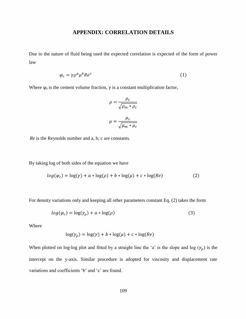
109

APPENDIX: CORRELATION DETAILS

Due to the nature of fluid being used the expected correlation is expected of the form of power

law

Where φc is the cement volume fraction, is a constant multiplication factor,

√

√

Re is the Reynolds number and a, b, c are constants.

By taking log of both sides of the equation we have

For density variations only and keeping all other parameters constant Eq. (2) takes the form

Where

When plotted on log-log plot and fitted by a straight line the ‘a’ is the slope and log ( ) is the

intercept on the y-axis. Similar procedure is adopted for viscosity and displacement rate

variations and coefficients ‘b’ and ‘c’ are found.

110

The plot of cement volume fraction against density, viscosity and displacement rate for vertical

concentric cases are shown in Figure 84.

Figure 84: Plots for spacer density, viscosity and Reynolds number variations

Procedure to Find R2 Value

Sum of squared error (SSE) = ∑

Total sum of squares (SSTo) = ∑

111

VITA

Muhammad Zulqarnain was born in Sargodha, Pakistan, in 1975. He completed his Master of

Science in Nuclear Engineering from Pakistan Institute of Engineering and Applied Science,

Islamabad, Pakistan, in 2003. After that he worked in a public sector organization in Pakistan for

four and half years. In August 2009, he joined The Craft and Hawkins Department of Petroleum

Engineering at Louisiana State University, Baton Rouge, Louisiana, for Master of Science. The

degree of Master of Science in Petroleum Engineering will be conferred in May 2012.

simulations of the primary cement placement in annular

Documents