simulations of non homogeneous viscous ows with
TRANSCRIPT

Simulations of non homogeneous viscous flows with
incompressibility constraints
Caterina Calgaroa, Emmanuel Creusea, Thierry Goudonb, Stella Krellb
aUniv. Lille, CNRS, UMR 8524 - Laboratoire Paul Painleve, F-59000 Lille, FrancebInria, Team COFFEE, Centre de recherche Sophia Antipolis Mediterrannee
& Universite Nice Sophia Antipolis, CNRS, & Laboratoire J. A. Dieudonne, UMR 7351,Parc Valrose, 06108 Nice cedex 02, France
Abstract
This presentation is an overview on the development of numerical methods forthe simulation of non homogeneous flows with incompressibility constraints.We are particularly interested in systems of partial differential equations de-scribing certain mixture flows, like the Kazhikhov–Smagulov system whichcan be used to model powder–snow avalanches. It turns out that the In-compressible Navier–Stokes system with variable density is a relevant steptowards the treatment of such models, and it allows us to bring out someinteresting numerical difficulties. We should handle equations of differenttypes, roughly speaking transport and diffusion equations. We present twostrategies based on time–splitting. The former relies on a hybrid approach,coupling finite volume and finite element methods. The latter extends dis-crete duality finite volume schemes for such non homogeneous flows. Themethods are confronted to exact solutions and to the simulation of Rayleigh–Taylor instabilities.
Keywords: Non homogeneous viscous flows, Navier–Stokes equations,Mixtures, Multifluid flows, Finite volume methods.
1. Introduction
The motivation of this work comes from the mathematical modelling ofmixtures or multifluid flows. In fact, there exists a large variety of partialdifferential equations (PDEs) systems intended to describe such flows, and,of course, we will focus on some specific models. The situations we areinterested in can be characterized by the following features:
Preprint submitted to Mathematics and Computers in Simulation April 3, 2016
• There are strong density variations in the flows, and the numericalchallenge is to capture and to follow with accuracy the strong gradientsand the fronts of density variations.
• The set of equations involves a constraint on the divergence of thevelocity field, hereafter denoted by u. The simplest of these constraintsis the solenoidal condition divx(u) = 0, but we shall see more intricatesituations.
Our objective consists in designing dedicated numerical methods for the sim-ulations of these models. The difficulty comes from the fact that the systemcouples equations of different type, and the constraint mentioned above. Theconstraint relies on modelling assumptions. In order to set up performingmethods, it could be helpful to understand the origin of this relation. Wewill give some hints in this direction. The discussion should be taken withfull awareness that many aspects in the derivation of the equations are notthat neat, and can be considered as questionable: mathematical models inthis field remain under debate. According to prescriptions in [60], our view-point is therefore fully pragmatic: let us say that we are just picking a setof equations, and we try to discuss some mathematical properties, and toset up specific numerical schemes that allow us to investigate the sensitiv-ity of the model with respect to variations of the (physical and numerical)parameters. However, we should bear in mind that the robustness of theconclusion should be considered with caution: changing a “detail” in themodelling assumptions might dramatically affect the mathematical structureof the model, which thus would require another approach.
Let us end this introduction with a few words about potential applicationsof our approaches. Powder–snow avalanches is a relevant example of the kindof fluid mixtures we are considering and variations about the Navier–Stokessystem have been used successfully to reproduce certain features of labora-tory avalanches [26, 27, 28]. These complex models also naturally arise incombustion theory; nuclear safety engineering provides further relevant ex-amples of applications, see for instance the works [24, 6, 59] motivated bysecurity computations for PWR reactors. Finally, we mention that the rea-sonings of mixture theory have been developed to derive models describingbiofilms formation [17].
The paper is organized as follows. We start by discussing a few relevantmathematical models that couple transport, diffusion and constraint equa-
2

tions. In Section 3 we present the hybrid finite volume (FV)–finite element(FE) scheme developed in [14, 12, 15]. The method is designed to reachthe second order accuracy, at least for smooth solutions, owing to a suitableadaptation of Monotonic Upstream-Centered Scheme for Conservation Laws(MUSCL) techniques for the transport equation. Here, we pay attention tothe treatment of the boundary conditions. Proceeding naively might leadto spurious instabilities when the geometry of the mesh and of the compu-tational domain is non trivial. An alternative numerical method based onthe Discrete Duality Finite Volume (DDFV) framework is introduced in Sec-tion 4. The DDFV framework is an attempt to cope with the difficulty indefining diffusion fluxes on interfaces without imposing geometric restrictionson the mesh construction, see [42, 43, 25]. The method has been extended todeal with Stokes and homogeneous Navier–Stokes equations [22, 47, 49, 48].Dealing with non homogeneous flows requires a specific attention to design arelevant treatment of the convection terms of the system [33]. Section 5 offersa set of numerical experiments where we compare the performances of thetwo methods. In particular, we bring out difficulties related to the treatmentof the boundary terms and the sensitivity to the mesh construction.
2. Examples of non–homogeneous flows involving constraints ondivx(u)
2.1. Incompressible flows
Let us start by recalling a few facts about the simplest situation of in-compressible flow which means that the velocity is required to satisfy
divx(u) = 0. (1)
Neglecting any difficulty associated to a possible lack of regularity of u :R×RN → RN , let us consider the characteristic curves, defined by the ODEsystem
d
dtX(t, x) = u(t,X(t, x)), X(0, x) = x.
The quantity X(t, x) ∈ RN is nothing but the position at time t ≥ 0 of aparticle, driven by the velocity field u, which starts at time t = 0 from theposition x ∈ RN . Let us consider a fixed domain D0, and consider its imageat a latter time t > 0
D(t) = X(t, x0), x0 ∈ D0.
3

D0 •x
D(t)
•X(t, x)
u(t,X(t, x))
Figure 1: Evolution of the domain D0.
(See Figure 1.) This is a simple exercice (see [32, Chap. 4]) to check that(1) implies
d
dt
(∫D(t)
dx
)= 0.
In other words, volumes are conserved by the flow.Next, let ρ : R× RN → [0,∞) stand for the mass density of the fluid. It
obeys the mass conservation equation
∂tρ+ divx(ρu) = 0.
Expanding the space derivative, and taking into account (1), we find
∂tρ+ u · ∇xρ+ ρ divx(u) = ∂tρ+ u · ∇xρ = 0.
Accordingly, the chain rule leads to
d
dt
[ρ(t,X(t, x))
]= 0.
The density is conserved along the characteristic curves, and we deduce that
ρ(t,X(t, x)) = ρ0(x).
4
As a particular case, an homogeneous fluid, satisfying ρ0(x) = ρ > 0 for anyx, remains homogeneous for ever. Coupled to the momentum equation, say1
∂t(ρu) + Divx(ρu⊗ u) +∇xp = µ∆u + ρf ,
where ρf is the density of applied forces and µ > 0 is the dynamic viscosityof the fluid, this is the case which is usually referred to as the IncompressibleNavier–Stokes system. The third unknown, the pressure p : R × RN →R, can be seen as a Lagrange multiplier associated to the constraint (1).However, there is no reason to restrict to homogeneous flows and we candeal with variable initial density as well. Compared to the huge literature onthe homogeneous Navier–Stokes system, there are only a few results on theanalysis of the Incompressible Navier–Stokes system with variable density,see e. g. [8, 20, 53] and a few attempts of numerical simulations of suchflows [14, 12, 37, 38, 44, 61]. Let us now discuss further models where moreintricate constraints appear.
2.2. Zero–Mach flows
The starting point of the discussion is the compressible Navier-Stokessystem
∂tρ+ divx(ρu) = 0,∂t(ρu) + Divx(ρu⊗ u) +∇xP = Divx(τ) + ρf ,∂t(ρE) + divx((ρE + P )u) = divx(k∇xT ) + divx(τu) + ρf · u,
with τ = µ(∇u +∇uᵀ− 23divx(u)I). Additionally to the mass density ρ and
the velocity field u, the unknowns involve the total energy E ≥ 0, which
splits into kinetic energy and internal energy E = |u|22
+ e with a state lawrelating e, P and ρ: P = RρT = (γ − 1)ρe, R being the constant of perfectgases and γ > 1 an exponent that characterizes the fluid under consideration.In order to write the equations in dimensionless form, we introduce density,time, length and velocity units ρ?,T,L, U = L/T respectively. Let E be theenergy unit and we define the temperature unit as γ−1
RE and the pressure
unit is P = ρ?E . We can now introduce the Mach number
Ma =U√E
=
√ρ?U
2
P.
1Here we adopt different notations for the divergence of a vector field divx(u) =∑Nj=1 ∂xj
uj and the divergence of a matrix-valued function [Divx(A)]i =∑Nj=1 ∂xj
Aij .
5

We assume that all the other dimensionless parameters — namely the Rey-nolds, Froude and Prandtl numbers2 — that characterize the flow have thesame order of magnitude and we consider the regime where the Mach numberis small:
Ma Re ' Fr ' Pr.
Keeping only Ma in the dimensionless form of the equation, we are led to
∂tρMa + divx(ρMauMa) = 0,
∂t(ρMauMa) + Divx(ρMauMa ⊗ uMa) +1
Ma2∇xPMa = Divx(τMa) + ρMaf ,
∂t(ρMaEMa) + divx((ρMaEMa + PMa)uMa)= divx(k∇xTMa) + Ma2(divx(τMauMa) + ρMaf · uMa).
Furthermore, the Mach number also enters into the definition of the totalenergy
EMa =Ma2
γ − 1
|uMa|2
2+
TMa
γ − 1, PMa = ρMaTMa. (2)
Let us assume that all unknowns admit limit ρ,u, T , etc... in a strongenough sense so that we can deal with the non linear terms. As Ma →0 the momentum equation degenerates to ∇xP = 0. Up to a convenientassumption on the boundary condition, we infer that the pressure does notdepend on time and space, namely we have ρT (t, x) = P? (constant). Themass conservation equation becomes ∂tρ + divx(ρu) = 0. Next, we multiplythe momentum equation by a divergence free trial function — namely avector valued function ϕ ∈ C∞c , with divx(ϕ) = 0 — in order to get rid ofthe stiff term (since
∫∇xPMa ·ϕ dx = −
∫PMadivx(ϕ) dx). Letting Ma→ 0
yields ∫ (∂t(ρu) + Divx(ρu⊗ u))− ρf −Divx(τ)
)·ϕ dx = 0, (3)
for any such trial function. Accordingly, we obtain
∂t(ρu) + Divx(ρu⊗ u) +∇xπ = ρf + Divx(τ),
2We remind the reader that these numbers are defined by Re = ρ?ULµ , Fr = U√
‖f‖L,
Pr = µρ?k
respectively, with µ, k and f typical values for the dynamic viscosity, the thermal
diffusivity and the force density (in most cases the latter is the gravity acceleration).
6

where the multiplier π appears as a consequence of the fact that (3) onlyholds for a restricted set of trial functions. We turn to the energy equation,bearing in mind (2). In particular ρMaEMa tends to 1
γ−1ρT = P?
γ−1. Therefore
the limiting energy equation reads
γP?γ − 1
divx(u) = divx(k∇xT ) = P?divx(k∇x(1/ρ)).
Namely, we obtain a constraint where the divergence of the velocity is relatedto derivatives of a function of the density. The analysis of such an asymptoticregime is quite challenging; we refer the reader to [2, 1].
Note that it is a different question to search for a numerical schemefor the limiting system only or to construct a method for the compress-ible model which is able to handle correctly the regime Ma 1 and whichavoids prohibitive stability conditions. On this aspect we refer the reader to[62, 23, 39, 40, 41, 65]. We also mention the derivation of further modelscorresponding to the Zero–Mach regime in [24, 6, 59].
2.3. Modelling of mixtures: the Kazhikhov–Smagulov system
We are interested in flows that can be seen as a mixture of a disperse phaseand a carrying phase, with respective mass densities ρd, ρf . Let ud,uf standfor their respective velocities. We start by writing the mass conservationequation for both phases:
∂tρd,f + divx(ρd,fud,f ) = 0. (4)
Adding these equations, we obtain
∂tρ+ divx(ρu) = 0, (5)
whereρ = ρd + ρf , ρu(t, x) = (ρfuf + ρdud)(t, x),
define the mean mass density ρ and the mean mass velocity u respectively.Next, we write the following momentum balance equation for ρu
∂t(ρu) + Divx(ρ u⊗ u) +∇xp = ρg + Divx(µD(u)),
with D(u) = ∇xu+∇xuᵀ. In the right side the force term ρg is proportional
to the gravitational field g. In order to close the equations, we need to explainhow the pressure field p is defined.
7

We bear in mind that we adopt an averaged description of the flow, wherewe consider that at each time t and each position x, the two phases can bepresent. The local amount of the disperse phase is evaluated through thevolume fraction 0 ≤ φ(t, x) ≤ 1, which can be intuitively thought of throughthe formula
φ(t, x) = limr→0
Volume occupied by the disperse phase in B(x, r)
|B(x, r)|.
The system is closed by specifying the modelling assumption. Here andbelow we assume the incompressibility of both phase, in the sense that, if asingle phase were occupying a given location, then its mass per unit volumeis constant (given by ρd, ρf ). Accordingly, we simply have
ρd(t, x) = ρdφ(t, x), ρf (t, x) = ρf (1− φ(t, x)).
Let us go back to (4) with this assumption. It yields
∂t
(ρfρf
+ρdρd
)= ∂t(1− φ+ φ) = 0 = −divx
( ρfufρf
+ρdudρd︸ ︷︷ ︸
:=v
).
It means that the mean volume velocity
v(t, x) =(1− φ(t, x)
)uf (t, x) + φ(t, x)ud(t, x),
is divergence-free.
Remark 2.1. The distinction between the mean volume velocity and themean mass velocity can be crucial in fluid mechanics: in a series of papersHoward Brenner [9, 10] proposed to revisit the derivation of Navier–Stokesequations based on this distinction. It turns out that this approach is highlycontroversial, see e. g. [54]. However, we point out that Brenner’s modelshave been showed to exhibit nice mathematical structure and stability prop-erties [29]. Moreover, similar corrections to the standard Navier–Stokes sys-tems have been proposed recently motivated by numerical purposes [36].
Having observed this fact, the system of PDEs is closed by assuming aFick’s law that relates the mean mass velocity u, the mean volume velocityv and gradient of the density ρ:
u = v − κ∇x ln(ρ), (6)
8

with a certain coefficient κ > 0. This assumption together with the fact thatv is solenoidal yields
divx(u) = −divx(κ∇x ln(ρ)).
It is worth remarking that the closure relation can be expressed equivalentlyon the carrier fluid velocity uf = u− κ1∇x ln(ρf/ρ) or as an evolution equa-tion, of convection–diffusion type, for the disperse volume fraction
∂tφ+ divx(φu) = divx(κ2∇x ln(ρf + (ρd − ρf )φ),
with positive coefficients κ1 or κ2. These observations lead to different op-tions to choose the numerical unknowns. However, the equivalence betweendifferent formulations, which is clear for the continuous equations, might failfor the corresponding discrete systems, see [7].
For the introduction of such models for mixtures, and application to pol-lution spreading, we refer the reader to Kazhikhov–Smagulov [46], see also[30, 31, 35, 45]. The analysis of this system dates back to [3, 4, 63]. Impos-ing a specific relation between the viscosity µ and the diffusion coefficient κfurther estimates (roughly speaking that control ∇xρ) can be derived whichare useful to justify the existence of solutions [11, 51, 52]. In [15, 34], wereinterpret the derivation of the KS equations by means of hydrodynamicregimes, starting from a coupled fluid–kinetic system. This viewpoint allowsus to derive a new model which can be interpreted as a generalized KS systemand which has remarkable dissipation properties.
2.3.1. A hierarchy of models
It looks tempting to get rid of u and to make use of the relation divx(v) =0, which is a more usual constraint. We plug (6) into (5); it makes a diffusionterm appear since
divx(ρ κ∇x ln(ρ)
)= κdivx
(ρ∇xρ
ρ
)= κ∆xρ.
9

Similarly, we rewrite the momentum equation with the mean volume velocityv instead of u, see [15]. We obtain the following system for ρ,v and p
∂tρ+ divx(ρv) = κ∆xρ,
ρ(∂tv + (v · ∇x)v
)+∇xp = ρg + Divx(µD(v))
+κ(∇xv −∇xvᵀ)∇xρ
+κ2(∇x∆xρ−Divx
(∇xρ⊗∇xρ
ρ
))−κDivx
(µD2
x ln(ρ)).
Choosing the mean volume velocity v instead of the mean mass velocityu has, at least, two consequences. Firstly, it changes the mass conserva-tion equation, which becomes a convection–diffusion equation instead of amere transport equation. Secondly it makes several ugly terms appear inthe momentum equation, that involve high–order derivatives of the density.Furthermore, in this form, we also realize that the “additional terms” induceintricate boundary conditions: in fact the Fick law hides further modellingissues related to the definition of the boundary conditions.
Let us point out that various simplifications are relevant:
• Assume a simple expression for µ, say constant or an affine function ofρ,
• Get rid of higher order terms by an asymptotic argument; as it appearsin [46],
• Assume an ad hoc relation between µ and κ: with µ = µ0 + µρ andκ = µ, the higher order terms cancel out and, furthermore a remarkableenergy identity can be established, as observed in [26, 11, 21, 52].
2.3.2. Example: simulations of powder–snow avalanches
Before entering into details of the numerical methods, let us discuss appli-cations of Kazhikhov–Smagulov (KS) equations to the description of powder–snow avalanches. To this end, we rewrite the system in the following dimen-
10
sionless form:
∂t ρ+ divx(ρv) =1
Re Sc∆x ρ,
ρ(∂tv + (v · ∇x)v
)+∇xp
=1
Fr2ρg +1
ReDivx(µ(ρ)D(v)) +
1
Re Sc(∇xv −∇xv
ᵀ)∇xρ,
divx(v) = 0,
where we make the following dimensionless parameters appear:
Reynolds number: Re =U L
ν,
Froude number: Fr = U(gL)−1/2,
Schmidt number: Sc =ν
κ.
Here, L and U stand for length and velocity units, respectively, g gives thevalue of the gravitational acceleration, while ν is a typical value of the kine-matic viscosity of the flow. Engineers also introduce the densimetric Froudenumber
Frd = U(gL
∆ρ
ρd
)−1/2
,
which also depends on the extreme densities within the flow ρd, with ∆ρ =ρf−ρd. Note that we have adopted the simplifying assumptions that allow usto get rid of terms with higher-order derivatives of the density. As a matterof fact, we remark that Sc = +∞ gives the usual Incompressible Navier–Stokes system. As said above, the system requires boundary conditions, onthe density and the velocity; in what follows, simulations are presented with
v∣∣∂Ω
= 0, ∇xρ · ~ν∣∣∂Ω
= 0,
where ~ν is the unit outward normal of the domain.
The mathematical modelling of powder–snow avalanches, like many othermixture flows, is still widely open. Nevertheless, we have at hand experi-mental data and numerical simulations (based on different systems of PDEsthough), which can be used to discuss the relevance of the results and the roleof the different parameters. We use experimental data obtained at Cemagref-IRSTEA [56, 57, 55, 19]. For real avalanches, we have Re ' 108, and Frd ' 1
11
which make this situation not affordable for simulation. But laboratoryavalanches have been produced with less extreme parameters: Re ' 103−104,Frd ' 1. Data are available but the comparison should still be consideredwith caution since many crucial parameters are not really well-known likethe Schmidt number Sc, the mass densities of the constituents, the viscos-ity coefficient of the mixture, etc. Further discussions would be necessaryon the boundary conditions to decide whether or not it is necessary to con-sider friction effects. Finally, the method and the quality of measurementscould be also questionable, with several sources of uncertainties. The ex-perimental results have been compared to simulations, performed on a k/εmodel, with tuned parameters, by using the Fluent software packages, onfixed Cartesian grids. Another set of simulations appeared in [27, 28], basedon a version of the KS system, with a Finite Element scheme coupled to char-acteristic methods for the convection terms; the simulations also use meshrefinements strategies in order to follow the advance of the front. Finally [26]uses OpenFoam, on a fixed Cartesian mesh to produce numerical avalanchesby using the KS system.
In [15], we simulate the KS system on the initial configuration representedin Figure 2. We use the hybrid FV-FE method described in Section 3, coupledto a mesh refinement method: see Figure 3 for a typical example of meshadapted to the displacement of the avalanche. We deal with different sets ofparameters:
• From numerical experiments in [26]
– Frd = 1, Fr = 4.3589, Re = 2242, Sc = 1.0.
– Mesh refinements go up to 15.000 triangles, with smallest convexradius hmin ≈ 7× 10⁻⁴m (the domain size is 2.7× 0.8m and theinitial avalanche size 0.3× 0.3m).
– We obtain very similar results (up to a slight change of units whichneed to be corrected in [26]).
• From laboratory experiments in [56, 57, 55, 19]
– Frd = 0.83, Fr = 0.3725, Re = 1000, Sc = 1.
– Mesh refinements go up to 50.000 triangles, with smallest convexradius hmin ≈ 1.5 × 10⁻⁴m and maximum length of the edgeshmax ≈ 10−2m (domain size 2 × 0.5m and initial height of theavalanche L= 0.09m).
12

– The order of magnitude of the horizontal velocity agrees with thevalue recorded form the experiments (0.35ms−1).
The simulations permit us to bring out the following qualitative results:
• Variations of Sc do not change significantly the velocity of the front.But the density profiles are modified: the KS model produces resultsnoticeably different from the mere incompressible system.
• Numerical difficulty increases as Re increases or Fr decreases.
• Numerical results are qualitatively consistent with the experiments.
• The Reynolds number affects the details of the flow, but does not sig-nificantly influence the speed of the front.
• The Froude number greatly influences maximal speeds.
• The maximal velocity exceeds the front speed by 30% to 40%.
h
l0ds
l
lshs
h0
θ
~g
ρ+, ν+
ρ−, ν−
ρ, ν
Figure 2: Domain and initial data configurations.
In the following sections, we are going to describe numerical strategies todeal with such equations, restricting to the simpler case of incompressible,but non–homogeneous, flows.
13

Figure 3: An adapted mesh that follows the avalanche front.
3. A hybrid finite volume–finite element scheme
3.1. Principles of the method
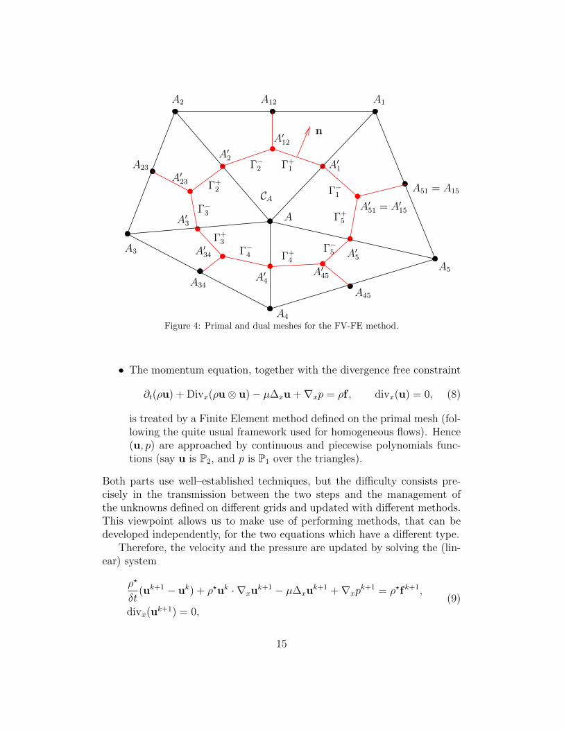
Let us start by discussing the numerical simulation of the incompressibleNavier–Stokes system in a two-dimensional domain Ω. We work with a (con-formal) tessellation τh made of triangles T , and we define Ωh = ∪T∈τhT . Letus note that in the case where Ω is a polygonal domain, then τh is definedsuch that Ωh = Ω whatever the tessellation τh chosen. We associate to thisprimal mesh a dual mesh: the vertices of the primal mesh are consideredas the centers of the cells of the dual mesh. As we shall see below, thereare several options to construct the dual mesh: in Figure 4 it is obtained byjoining the barycenters of the triangles to the middle of the edges.
Our scheme works by time–splitting the mass conservation and the mo-mentum balance equation and by dealing with the equations on staggeredgrids defined on Ωh :
• The mass conservation
∂tρ+ divx(ρu) = 0, (7)
is treated by a finite volume method, with cells defined by the dualmesh;
14
A1A2
A3
A4
A5
A12
A23
A34A45
A51 = A15
A
CA
A′1
A′12
A′2
A′23
A′3
A′34
A′4A′45
A′5
A′51 = A′15
Γ−1
Γ+1Γ−2
Γ+2
Γ−3
Γ+3
Γ−4 Γ+4
Γ−5
Γ+5
n
Figure 4: Primal and dual meshes for the FV-FE method.
• The momentum equation, together with the divergence free constraint
∂t(ρu) + Divx(ρu⊗ u)− µ∆xu +∇xp = ρf , divx(u) = 0, (8)
is treated by a Finite Element method defined on the primal mesh (fol-lowing the quite usual framework used for homogeneous flows). Hence(u, p) are approached by continuous and piecewise polynomials func-tions (say u is P2, and p is P1 over the triangles).
Both parts use well–established techniques, but the difficulty consists pre-cisely in the transmission between the two steps and the management ofthe unknowns defined on different grids and updated with different methods.This viewpoint allows us to make use of performing methods, that can bedeveloped independently, for the two equations which have a different type.
Therefore, the velocity and the pressure are updated by solving the (lin-ear) system
ρ?
δt(uk+1 − uk) + ρ?uk · ∇xu
k+1 − µ∆xuk+1 +∇xp
k+1 = ρ?fk+1,
divx(uk+1) = 0,
(9)
15

where we are faced the question of how to define the density ρ? to be used inthe FE scheme to compute u. To this end, we have at hand a density fieldwhich is constant over the control volumes. Thus, given a triangle, we know 3values of densities (ρk+1); hence we can naturally define a P1 reconstruction:this is the ρ? that arises in (9).
The update of (u, p) can be seen as a saddle point problem which, oncediscretized with respect to space, is expressed in the following matrix form(
A BBT 0
)(uk+1
pk+1
)=
(ρ?fk+1
0
).
We point out that non homogeneities of the flows make the structure of thematrix A more complicated since ρ? varies from place to place. If we thinkin terms of the underlying elliptic equation for the pressure (as usual whenusing projection methods), this equation is now with variable coefficients,which might lead to preconditioning issues, see [13].
The discussion of the mass conservation equation is more subtle. Weconsider a control volume CA with center A (see Figure 4). The numericalunknown ρkA is intended to approximate 1
|CA|
∫CAρ(tk, x) dx. Integrating the
the mass conservation equation over CA yields
ρk+1A − ρkAδt
+1
|CA|∑i
∫Γi
ρku · n dσ(x) = 0,
where ∂CA = ∪nbi=1Γi, with Γi = Γ+i ∪ Γ−i , nb the number of neighbour nodes
of A (respectively denoted Ai, 1 ≤ i ≤ nb), and n the unit outward normalto ∂CA. Here, we address the question, given u piecewise polynomial on thetriangles, to define a suitable u?, piecewise constant on ∂CA, to obtain arelevant approximation of u? · n on ∂CA.
To construct the numerical flux, the basic requirement is to preservehomogeneous states: if ρ is constant over the whole computational domain,it should remain constant forever. The naive construction which simply usesthe evaluation of the FE function u, P2 per triangle, on the interface ∂CA,fails to meet this objective, and we propose another construction. We bearin mind that the divergence free condition for the FE method actually reads∫
ωA
divx(u)ψA dx = 0 =∑i
∫Ti
divx(u)ψA dx,
16

for all P1 basis function ψA associated to the node A with supp(ψA) = ωA =∪nbi=1Ti. It turns out that this formula does not involve the value of u at thenodes Ai, but only at the nodes A′i and Aii+1 (1 ≤ i ≤ nb), corresponding tothe degrees of freedom associated to the middle of the edges. Thus, we seeku?+i =u?−i+1 the velocity on Γ+
i ∪ Γ−i+1 , as a convex combination of ui,i+1 , u′iand u′i+1 such that :∑
i
(|Γ−i |u?−i · n|Γ−i + |Γ+
i |u?+i · n|Γ+i
)= 0,
this expression corresponding to the finite volume interpretation of the di-vergence free condition. It yields some algebraic relations and we end upwith
u?+i = u?−i+1 =1
3
(u′i + ui,i+1 + u′i+1
).
As a matter of fact it is worth observing that
• u?+i 6= u(A′i i+1),
• The formula for u?+i coincides with a linear interpolation at A′i i+1 fromu at the nodes A′i, A
′i+1 and Ai i+1.
With the value of u?+i at hand, a simple upwind finite volume schemewould naturally lead to
∫Γ+i
ρku · n dσ(x) =
ρkA |Γ+
i |u?+i · n if u?+i · n > 0,
ρkAi |Γ+i |u?+i · n if u?+i · n < 0,
(10)
and ∫Γ−i+1
ρku · n dσ(x) =
ρkA |Γ−i+1|u?−i+1 · n if u?−i+1 · n > 0,
ρkAi+1|Γ−i+1|u?−i+1 · n if u?−i+1 · n < 0.
(11)
3.2. Extension: MUSCL scheme on unstructured meshes, maximum princi-ple and multislope methods
Using upwind fluxes such as (10) and (11) restricts the method to firstorder accuracy. To improve the accuracy, fluxes can be designed based onMUSCL strategies. While the method is completely clear in 1D or on Carte-sian grids, difficulties arise when dealing with general unstructured meshes.
17

Following ideas introduced in [18, 16] for Cell–Center methods, we designa multislope method for Vertex–Based methods, defining directional deriva-tives and limiters on each interfaces. We refer the reader to Figure 5, and wefocus on the treatment to be done on Γ+
1 . A similar reasoning applies to allthe other components of ∂CA. Let us denote n+
1 the unit outward normal ofCA on Γ+
1 and let us suppose that u?+1 · n+1 > 0. Let A+
1 be the mid–point of[A′1A
′12]. Our goal is to derive the value of ρk
A+1
, to be used instead of ρkA in
the definition of the flux (10), in order to increase the accuracy of the FiniteVolume scheme. Let M+
1 and N+1 be the two intersection points between
(AA+1 ) and ∂ωA (see Figure 5). We define
pup,+1 =
ρA − ρN+1
‖AN+1 ‖
,
and
pdown,+1 =
ρM+1− ρA
‖AM+1 ‖
.
Then the density is evaluated at node A+1 by
ρA+1
= ρA + p+1 ‖AA+
1 ‖,
with
p+1 = pup,+
1 Lim(pdown,+
1
pup,+1
),
where Lim is a so-called ”τ -limiter”. For the convection equation, the L∞
stability of the scheme can be established and improved accuracy is observedon numerical validations, see [12]. Eventually, the method can be coupled tomesh-refinement algorithms in order to follow strong density gradients. Thisscheme has been adapted to handle the additional terms of the KS systemand to perform the computations of the numerical avalanches, see [15].
3.3. Boundary conditions
The treatment of boundary conditions is seldom addressed in details.However, it gives rise to important practical issues, in particular when we
18

A
A1A2
A5
M+1
N+1
A3
A4
T1
T5
n+1
A′1
A′12
A+1
Γ+1
Figure 5: Construction of the upstream and downstream gradients for the definition ofmultislope limiters.
wish to maintain a high-order accuracy. We distinguish the cases of “Dirich-let” or “Neumann” boundary conditions to be imposed on the density. Theformer refers to the usual situation where the inflow density is imposed:
ρ(t, x) = ρb(t, x) for (t, x) ∈ (0, T )× ∂Ω such that u · ~ν < 0.
In this case, we just specify the prescribed value at the boundary ∂Ωh. Asclassically known, the approximation of the exact value of ρb on ∂Ω givenby an interpolated value ρh on ∂Ωh introduces an additional error of or-der O(h2). The latter refers to another common situation where either theboundary condition is intended to describe the reflection of the fluid by theboundary ∂Ω (wall boundary conditions) or it accounts for symmetry con-ditions, which are used to reduce the computational domain. This situationoccurs for instance with the simulation of Rayleigh–Taylor instabilities, thatwill be presented in Section 5. We are going to discuss how the numericalfluxes should be adapted to this situation, in the MUSCL framework pre-sented above.
We refer the reader to Figure 6: we focus on the cell with center A ∈∂Ωh, where the segments [A2A] and [AA5] of the primal mesh belong to the
19

boundary ∂Ωh. The flux through ∂Ωh ∩ ∂CA is evaluated as mentionned in[14]. In particular, the normal velocity at the boundary has to be carefullyevaluated, see [14, Section 2.4.3]. According to its sign, the normal flux ofthe density is evaluated from the numerical solution (outgoing flux) or byusing the boundary condition (incoming flux). Obviously, in the degeneratecase u? · nA = 0, no flux is added. However, it remains to evaluate theflux density on the interior interfaces of ∂CA: for instance on Γ+
1 we need todefine the value of ρA+
1. Going back to the construction in Section 3.2, the
difficulty comes from the definition of the upstream gradient pup,+1 since thenode N+
1 does not exist. A first solution is to let the scheme degenerate atorder one, by simply setting ρA+
1= ρA. We will see in Section 5 that this loss
of accuracy can generate instabilities in the close vicinity of the boundary,leading for some configurations to unphysical phenomena. This effect issensitive to the geometry of the domain and the shape of the mesh. As analternative, we propose a reflection technique, which uses a suitable definitionof “ghost cells”, see Figure 6 which can be easily generalized for other meshconfigurations. This method preserves the second order accuracy, as it willbe shown by the numerical experiments. Let nA be the unit outward vectorto ∂Ω at A, and let (NA) be its orthogonal line at A. We define A2, A1 andA5 as the points orthogonally symmetric with respect to (NA) of A2, A1 andA5 respectively. Consequently this construction defines the ghost trianglesT1 and T5. In order to enforce homogeneous Neumann boundary conditionsfor ρ on ∂Ω, we set ρA2
= ρA2 , ρA1= ρA1 and ρA5
= ρA5 . Going back to thedefinition in Section 3.2, it allows us to define an upstream gradient, by usingnow the value of the density defined by linear interpolation at the fictitiousnode N+
1 .
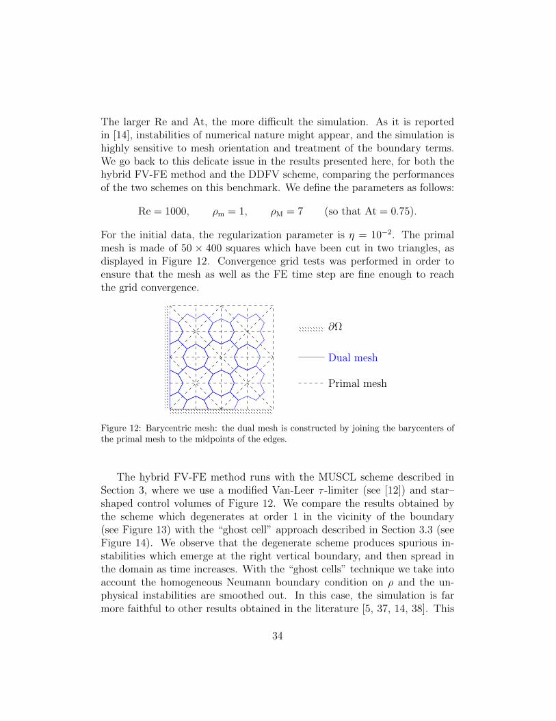
Remark 3.1. The geometry of the domain and the shape of the control vol-ume are important in this discussion. In [14] some simulations are performedby considering a mesh obtained by cutting through diagonals a preliminarytessellation made of squares, see Figure 12 below. On this structured mesh,control volumes of the dual mesh can be obtained by joining directly the mid-
20

A
A1A2
A5
A2
A1
A5
∂Ω
∂Ω
M+1
N+1
T1
T5T1
T5
n+1
A+1
Γ+1
nA
(NA)
Figure 6: Definition of the boundary condition.
points of the vertices of the triangles, see [14, Fig. 2-(b)]. For this veryspecific mesh, the two options actually coincide. Indeed, using the ghostcells, we find that the upstream and downstream gradients, in the normaldirection, are exactly the opposite of each other, and the limiter makes thescheme degenerate to first order.
4. A DDFV method for non homogeneous viscous flows
Still having in mind the possible adaptations to handle complex modelswith non homogeneous constraints, let us describe another approach, wherethe mass conservation and the momentum balance equations are both treatedby a finite volume method. It offers the advantage of a unified viewpoint inthe discretization method. To this end we adopt the Discrete Duality FiniteVolume (DDFV) framework, which, again, leads to consider unknowns onstaggered grids. When approximating diffusion equations by a finite volumeapproach, we face the difficulty of defining the normal derivative at the in-terfaces of the control volumes. Except in very specific geometric situations,the information stored at the center of the volumes is not enough for thatpurpose. After a pioneering attempt of Y. Coudiere, J.-P. Vila, P. Villedieu,
21

the basis of the DDFV method has been set up by F. Hermeline [42, 43] andK. Domelevo, P. Omnes [25]. The idea is two–fold: we increase the numberof numerical unknowns so that a full discrete gradient can be defined, and wedefine discrete operators so that the usual duality formula that are obtainedby integration by parts at the continuous level, are preserved. Since then,it has been the object of many extensions, including for the Stokes system[22, 47, 49, 48]. There exists also 3D versions of the method [50], which opensperspectives to deal with our scheme for non homogeneous flows in higherdimension as well.
4.1. Definition of the meshes and discrete operators
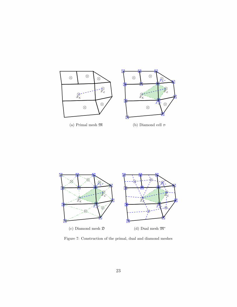
We refer the reader to [47, 48] for an exhaustive description of the nota-tions of the DDFV method. Let us explain the construction of the meshes.We start with a tessellation, the so-called primal mesh denoted by M. Itsconstruction can be quite general: we can mix triangles and quadrangles, pos-sibly with non–conformal elements, etc: see Figure 7-(a). With unknownsstored at xK and xL (the center of the control volume K and L) we can con-struct a discrete gradient, in the direction xK, xL; but since xK, xL is notassumed to be orthogonal to the interface of the control volume, this isnot enough to define the normal derivative at the interface. Therefore, weadditionally consider numerical unknowns stored at the vertices xK∗ , see Fig-ure 7-(b). Now, the subdomain defined by the four vertices xK, xK∗ , xL, xL∗
defines another control volume, the so–called diamond cell D. The tessella-tion obtained this way is referred to as the diamond mesh D; it is representedon Figure 7-(c). Finally, since we are dealing with unknowns stored at thevertices xK∗ of the primal mesh, we need to construct a control volume K∗
associated to these points. This is the dual mesh M∗ that can be obtainedeither by joining the centers xK of the primal mesh, see Figure 7-(d), or byjoining the centers xK to the mid-point of the edges.
In what follows, we denote by T = (M,M∗) the sets of primal and dualcells. Given a cell C (resp. an edge), mC stands for the volume of this cell(resp. the length of the edge). The velocity unknowns will be stored onthe primal uM = (uK)K∈M and dual uM∗ = (uK∗)K∗∈M∗ meshes: we shalldenote uT = (uM,uM∗). The pressure and density unknowns will be storedon the diamond mesh: ρD = (ρD)D∈D and pD = (pD)D∈D respectively. Next,we introduce discrete differential operators. Given a diamond cell D whosevertices are xK, xK∗ , xL, xL∗ , we can define discrete derivatives in the directions
22
⊗⊗
⊗⊗
⊗⊗ ⊗
xK
xL
(a) Primal mesh M
⊗⊗
⊗⊗
⊗⊗ ⊗
xK
xL
xK∗
xL∗
(b) Diamond cell D
⊗⊗
⊗⊗
⊗⊗ ⊗
xK
xL
xK∗
xL∗
(c) Diamond mesh D
⊗⊗
⊗⊗
⊗⊗ ⊗
xK
xL
xK∗
xL∗
(d) Dual mesh M∗
Figure 7: Construction of the primal, dual and diamond meshes
23
xK, xL and xK∗ , xL∗ :
∇DuT (xL − xK) = uL − uK,∇DuT (xL∗ − xK∗) = uL∗ − uK∗ .
Since the vectors xK, xL and xK∗ , xL∗ are not colinear, we can reconstruct,from uT defined on the dual and primal meshes, a full discrete Jacobianmatrix, defined on the diamond mesh:
∇DuT =1
2mD
[mσ(uL − uK)⊗~nσK +mσ∗(uL∗ − uK∗)⊗~nσ∗K∗
],
with mσ (resp. mσ∗) the length of (xK∗ , xL∗) (resp. (xK, xL)), ~nσK the unitvector orthogonal to the oriented edge σ = [xK∗ , xL∗ ], etc. The viscous termin the Navier–Stokes equation involves the symmetric part of this matrix,and the divergence can be defined as the trace:
DDuT = 12
(∇DuT + (∇DuT )ᵀ) ,divDuT = Tr
(∇DuT
).
Next, in order to obtain a discrete analog of the Stokes formula we introducethe discrete dual operator
divKξD :=1
mK
∑D∈DK
mσξD~nσK,
which picks a matrix–valued quantity defined on the diamond mesh, andreturns a vector defined on the primal and dual cells.
4.2. Treatment of the convection equation
Let us start by explaining how we handle the mass conservation equation.We remind the reader that the discrete mass density is intended to be anapproximation of the average over the diamond cells
∫D ρ(t, x) dx. Therefore,
we wish to mimic the flux∫D
div(ρu) =∑
s∈∂D
∫s
ρu ·~nsD.
By using the simplest upwind fluxes, we introduce the operator
divcD : RD ×(R2)T → RD,
24

⊗
⊗
⊗
D
D′
~nsD
s
xL∗
xK∗
xK
xL
Figure 8: The definition of the gradient on the diamond mesh uses the unknowns storedat the nodes xK, xL, xK∗ , xL∗ .
which depends on a density field given on D and a velocity field given on T ,defined by
mDdivcD(ρD,uT ) =∑
s∈∂DFs,D
Fs,D = ms
((us,D)+ ρD − (us,D)− ρD′
)where
us,D =uK + uK∗
2·~nsD for s = [xK, xK∗ ] ∈ ∂D,
with the standard notation x+ = max(x, 0), x− = −min(x, 0).Going back to the definition of the previous section, we observe that
divDuT =1
mD
∑s∈∂D
msus,D.
We deduce that the following consistency relation holds
divDuT = divcD(1D,uT ). (12)
The scheme for the mass conservation equation then reads
ρn+1D − ρnDδt
+ divcD(ρnD,unT ) = 0. (13)
Let us bring out two crucial properties of the scheme:
25

• We can identify a stability condition in order to preserve the positivityof the discrete density:
if ρnD ≥ 0 and δt ≤(‖uT ‖∞
1
mD
∑s∈∂D
ms
)−1
then ρn+1D ≥ 0.
• As a consequence of (12), we notice that divergence free velocity fieldspreserve homogeneous states: if ρnD ≡ 1 and divDunT = 0 then ρn+1
D ≡ 1.
Having at hand the discrete density piecewise constant on the diamondmesh D, we can naturally define the density on the primal and dual meshesby projection:
ρn+1K =
1
mK
∑D∈DK
m(D ∩ K)ρn+1D , ρn+1
K∗ =1
mK∗
∑D∈DK∗
m(D ∩ K∗)ρn+1D ,
for all K ∈ M, K∗ ∈ M∗. These quantities will be useful to deal with themomentum equation.
4.3. Treating the convection term in the momentum equation by taking intoaccount the constraint
The viscous term in the momentum equation is handled by standarddefinition of the DDFV framework for diffusion operator, see Section 4.1;similarly, for the pressure term, we refer the reader to [47, 48]. What isoriginal in this approach is the treatment of the convection term∫
Kdiv(ρu⊗ u) =
∑σ∈∂K
∫σ
(ρu · ~n)u.
It looks like “the transport of u by ρu”: this intuition guides the upwindingstrategy. At the discrete level, bearing in mind upwinding principles, we areled to introduce bT : RD × (R2)
T × (R2)T 7→ (R2)
T
bK(ρD,vT ,uT ) =1
mK
∑σ∈∂K
((FK,σ(ρD,vT )
)+uK −
(FK,σ(ρD,vT )
)−uL
)with the momentum flux
FK,σ = −m(D ∩ L)mD
∑s∈∂D,s⊂K
Fs,D +m(D ∩ K)
mD
∑s∈∂D,s⊂L
Fs,D.
26
⊗
⊗
FK,σ
Fs,D
xL∗
xK∗
xL
xK
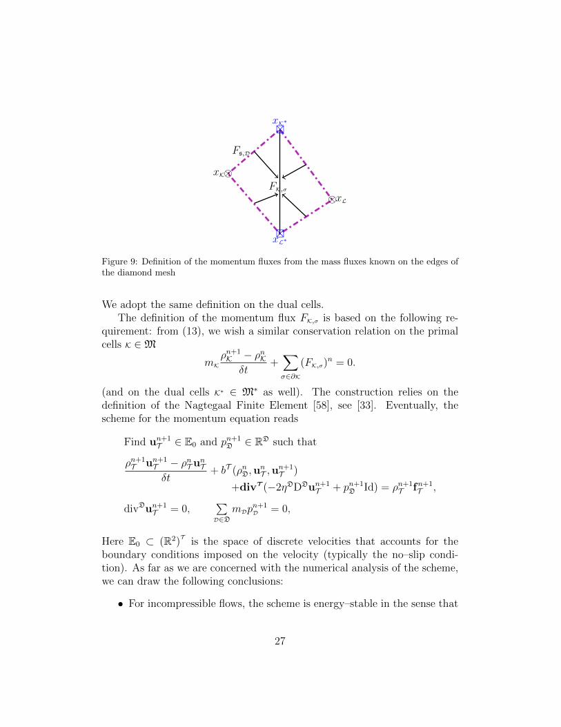
Figure 9: Definition of the momentum fluxes from the mass fluxes known on the edges ofthe diamond mesh
We adopt the same definition on the dual cells.The definition of the momentum flux FK,σ is based on the following re-
quirement: from (13), we wish a similar conservation relation on the primalcells K ∈M
mKρn+1K − ρnKδt
+∑σ∈∂K
(FK,σ)n = 0.
(and on the dual cells K∗ ∈ M∗ as well). The construction relies on thedefinition of the Nagtegaal Finite Element [58], see [33]. Eventually, thescheme for the momentum equation reads
Find un+1T ∈ E0 and pn+1
D ∈ RD such that
ρn+1T un+1
T − ρnT unTδt
+ bT (ρnD,unT ,u
n+1T )
+divT (−2ηDDDun+1T + pn+1
D Id) = ρn+1T fn+1
T ,
divDun+1T = 0,
∑D∈D
mDpn+1D = 0,
Here E0 ⊂ (R2)T
is the space of discrete velocities that accounts for theboundary conditions imposed on the velocity (typically the no–slip condi-tion). As far as we are concerned with the numerical analysis of the scheme,we can draw the following conclusions:
• For incompressible flows, the scheme is energy–stable in the sense that
27
it satisfies the following analog of the energy inequality
1
2δt‖√ρn+1T un+1
T ‖2T −
1
2δt‖√ρnT unT ‖2
T +1
2δt‖√ρnT (un+1
T − unT )‖2T
+Cη|||∇Dun+1T |||
22 ≤ Jρn+1
T fn+1T ,un+1
T KT .
• The scheme is semi–implicit, and to update the velocity and pressurerequires to solve a linear system: the invertibility of the system can beestablished and the solution (un+1
T , pn+1D ) is indeed uniquely defined.
• The approach does not use the fact that u is solenoidal and it can beadapted to any constraint that prescribes the divergence of the velocityfield.
Remark 4.1. Note that the treatment of the momentum equation differsfrom the viewpoint adopted with the hybrid VF-FE scheme: in (9), we dealtwith the discretization of the non–conservative form of the equation, involvingρ(∂tu + u · ∇u), while the DDFV scheme approaches the conservative term∂t(ρu) + Divx(ρu⊗ u).
5. Numerical validation
Before starting the discussion on numerical grounds, it is worth comparingthe degrees of freedom of the two methods, for 2D simulations. We considertessellations made of triangles, with unknowns stored at the edges E, thevertices V and the barycenters T according to the following table
Hybrid DDFVVelocity V & E V & TPressure V EDensity V E
Asymptotically we have #E ' 32
#T and #V ' 12#T . Since we deal with
two components for the velocity we get
DoFHybrid ' 5#T, DoFDDFV ' 6#T.
28
5.1. Analytical test
We first evaluate the abilities of the schemes to recover an analyticalsolution and we check the rate of convergence for the two methods. Let Ωbe the unit disk of R2. We consider the function defined in polar coordinates(r, θ) by
ρex(t, r, θ) = 2 + (2r − r2)e0.1(r2−2r) cos(θ − sin t),
uex(t, r, θ) =
(−r sin θ cos tr cos θ cos t
),
pex(t, r, θ) = sin(r cos θ) sin(r sin θ) sin(t).
It is an exact solution of the variable density incompressible Navier-Stokessystem (7)-(8) on Ω (with source term chosen accordingly). Compared withthe analytical solution used in [14] and [37], it should be noted that thissolution obeys now
∂ρex∂r
(t, r, θ) = 0 on ∂Ω.
This manufactured solution permits us to evaluate the efficiency of the methoddeveloped in Section 3.3 in order to take into account the homogeneous Neu-mann boundary condition.
We consider the disk Ω approximated by a polygonal domain Ωh anddiscretized with two isotropic unstructured meshes :
(A) either the mesh has some symmetry properties (Figure 10, left),
(B) or the unstructured mesh is more general (Figure 10, right).
For this solution, we have u · ~ν = 0 on ∂Ω where ~ν is the unit outwardnormal to Ω, but u · ~ν 6= 0 on ∂Ωh, and the normal flux of the densityshould be evaluated on the interfaces that intersect the boundary ∂Ωh. Forthe results discussed below, with the hybrid FV-FE method the dual meshis constructed as in Figure 12 (barycentric mesh, joining barycenters of theprimal mesh to midpoints of the edges). For the DDFV scheme we use asdual mesh either the barycentric mesh in Figure 12 or the classical mesh inFigure 15 (joining directly the barycenters of the primal cells); the resultsare not substantially different.
We plot the maximum error in time evaluated in L2(Ω) norm in spaceversus the number of cells (a half of the number of triangles) on the density,
29

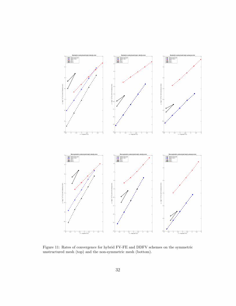
velocity and pressure. The top of Figure 11 corresponds to simulations madeusing the mesh (A) and the bottom of Figure 11 to those made using the mesh(B). The errors are plotted for the DDFV scheme and for the two differentstrategies on the boundary when we use the hybrid FV-FE method. The linescorresponding to a rate of convergence of order one (slope 1) and order two(slope 2) are also displayed. The computations are performed until the finaltime T = 1. In the FV-FE scheme, we choose δtFE = hmax and we computeδtFV ≤ δtFE in order to verify the CFL condition, see [12, Section 3.2]. Inthe DDFV scheme, the time step is similarly driven by the stability conditionof the convection operator.
In particular, for the FV-FE scheme, we compare the treatment of theboundary conditions using the ”ghost cells” or letting the MUSCL schemedegenerate at order one. For the density, the convergence rates (obtainedby linear regression) are respectively of order 1.69 for cases (A) and 1.76 forcase (B) if we adopt the strategy presented in Section 3.3. With the naiveapproach, the convergence rates decrease at order 1.42 for case (A) and 1.53for case (B). Despite this loss of accuracy on the density, we observe thatthe convergence rates for velocity and pressure remain optimal (order 2, andthe error curves for the degenerate and the ghost cells methods coincide).The degradation of the rates of convergence for the density, which are alwayssmaller than 2, is also due to the topology of the unstructured meshes andthe phenomenon is well known in the finite volume literature. On the onehand, the orders remains very satisfactory when we introduce the ”ghostcells” and they are very similar to those obtained in [14] for an analyticalsolution with Dirichlet boundary conditions. One the other hand, we notethat a loss of accuracy in the close vicinity of the boundary eventually leadsto a degraded performance of the scheme, even if the order remains higherthan one. The DDFV scheme is of order 1 for both the density and thevelocity, and a surprisingly higher accuracy for the pressure. In fact we notethat the rates are slightly better on coarse grids.
5.2. Rayleigh-Taylor instability
This Section is concerned with the numerical simulation of a Rayleigh-Taylor instability. This problem has been considered in numerous papers (see[64] for the inviscid case or [5, 37, 38, 14] for viscous fluids). We consider the
30
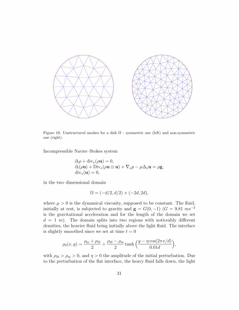
Figure 10: Unstructured meshes for a disk Ω : symmetric one (left) and non-symmetricone (right).
Incompressible Navier–Stokes system
∂tρ+ divx(ρu) = 0,∂t(ρu) + Divx(ρu⊗ u) +∇xp− µ∆xu = ρg,divx(u) = 0,
in the two–dimensional domain
Ω = (−d/2, d/2)× (−2d, 2d),
where µ > 0 is the dynamical viscosity, supposed to be constant. The fluid,initially at rest, is subjected to gravity and g = G(0,−1) (G = 9.81 ms−2
is the gravitational acceleration and for the length of the domain we setd = 1 m). The domain splits into two regions with noticeably differentdensities, the heavier fluid being initially above the light fluid. The interfaceis slightly smoothed since we set at time t = 0
ρ0(x, y) =ρm + ρM
2+ρM − ρm
2tanh
(y − η cos(2πx/d)
0.01d
),
with ρM > ρm > 0, and η > 0 the amplitude of the initial perturbation. Dueto the perturbation of the flat interface, the heavy fluid falls down, the light
31
-5.5 -5 -4.5 -4 -3.5 -3 -2.5 -2
x = -log(sqrt(T/2))
-10
-9
-8
-7
-6
-5
-4
-3
y =
lo
g(L
∞
(L2(Ω
)) n
orm
of
de
nsity e
rro
r)
Symmetric unstructured mesh, density error
MUSCL ghost cellsMUSCL order 1DDFVslope 1slope 2
-5.5 -5 -4.5 -4 -3.5 -3 -2.5 -2
x = -log(sqrt(T/2))
-14
-13
-12
-11
-10
-9
-8
-7
-6
-5
-4
y =
lo
g(L
∞
(L2(Ω
)) n
orm
of
ve
locity e
rro
r)
Symmetric unstructured mesh, velocity error
MUSCL ghost cellsMUSCL order 1DDFVslope 1slope 2
-5.5 -5 -4.5 -4 -3.5 -3 -2.5 -2
x = -log(sqrt(T/2))
-12
-10
-8
-6
-4
-2
0
2
y =
lo
g(L
∞
(L2(Ω
)) n
orm
of
pre
ssu
re e
rro
r)
Symmetric unstructured mesh, pressure error
MUSCL ghost cellsMUSCL order 1DDFVslope 1slope 2
-6 -5.5 -5 -4.5 -4 -3.5 -3 -2.5 -2
x = -log(sqrt(T/2))
-11
-10
-9
-8
-7
-6
-5
-4
-3
y =
lo
g(L
∞
(L2(Ω
)) n
orm
of
de
nsity e
rro
r)
Non-symmetric unstructured mesh, density error
MUSCL ghost cellsMUSCL order 1DDFVslope 1slope 2
-6 -5.5 -5 -4.5 -4 -3.5 -3 -2.5 -2
x = -log(sqrt(T/2))
-14
-13
-12
-11
-10
-9
-8
-7
-6
-5
y =
lo
g(L
∞
(L2(Ω
)) n
orm
of
ve
locity e
rro
r)
Non-symmetric unstructured mesh, velocity error
MUSCL ghost cellsMUSCL order 1DDFVslope 1slope 2
-6 -5.5 -5 -4.5 -4 -3.5 -3 -2.5 -2
x = -log(sqrt(T/2))
-10
-8
-6
-4
-2
0
2
y =
lo
g(L
∞
(L2(Ω
)) n
orm
of
pre
ssu
re e
rro
r)
Non-symmetric unstructured mesh, pressure error
MUSCL ghost cellsMUSCL order 1DDFVslope 1slope 2
Figure 11: Rates of convergence for hybrid FV-FE and DDFV schemes on the symmetricunstructured mesh (top) and the non-symmetric mesh (bottom).
32

fluid moves up, with the formation of a typical mushroom shape. Let usrewrite the equation in dimensionless form. To this end we choose d as thelength scale, while the time unit is defined by
T =
√d
G.
For the velocity unit we set U =d
T. The Reynolds number is then given by
Re =ρmd
3/2G1/2
µ.
Up to an obvious change of notations, we arrive at
∂tρ+ divx(ρu) = 0,
∂t(ρu) + Divx(ρu⊗ u) +∇xp−1
Re∆xu = −ρ
(01
),
divx(u) = 0,
in the two–dimensional domain Ω = (−1/2, 1/2) × (−2, 2). The problem issupplemented by no-slip boundary conditions on the horizontal boundaries.Actually, the solution has symmetries and we compute the solution on thehalf domain (0, 1/2)× (−2, 2) with the following boundary conditions for thevelocity field: denoting u = (u, v), we impose
On the horizontal boundaries: u = 0, v = 0,On the vertical boundaries: u = 0, ∂xv = 0.
The symmetry implicitly induces the Neumann boundary condition for thedensity. The difficulty of the problem essentially depends on
• the Reynolds number,
• the density ratio between the light and the heavy fluid, which is mea-sured by the so-called Atwood number
At =ρM − ρm
ρM + ρm
.
33
The larger Re and At, the more difficult the simulation. As it is reportedin [14], instabilities of numerical nature might appear, and the simulation ishighly sensitive to mesh orientation and treatment of the boundary terms.We go back to this delicate issue in the results presented here, for both thehybrid FV-FE method and the DDFV scheme, comparing the performancesof the two schemes on this benchmark. We define the parameters as follows:
Re = 1000, ρm = 1, ρM = 7 (so that At = 0.75).
For the initial data, the regularization parameter is η = 10−2. The primalmesh is made of 50 × 400 squares which have been cut in two triangles, asdisplayed in Figure 12. Convergence grid tests was performed in order toensure that the mesh as well as the FE time step are fine enough to reachthe grid convergence.
Primal mesh
Dual mesh
∂Ω
Figure 12: Barycentric mesh: the dual mesh is constructed by joining the barycenters ofthe primal mesh to the midpoints of the edges.
The hybrid FV-FE method runs with the MUSCL scheme described inSection 3, where we use a modified Van-Leer τ -limiter (see [12]) and star–shaped control volumes of Figure 12. We compare the results obtained bythe scheme which degenerates at order 1 in the vicinity of the boundary(see Figure 13) with the “ghost cell” approach described in Section 3.3 (seeFigure 14). We observe that the degenerate scheme produces spurious in-stabilities which emerge at the right vertical boundary, and then spread inthe domain as time increases. With the “ghost cells” technique we take intoaccount the homogeneous Neumann boundary condition on ρ and the un-physical instabilities are smoothed out. In this case, the simulation is farmore faithful to other results obtained in the literature [5, 37, 14, 38]. This
34

effect relies on the shape of the control volumes: the simulation in [14, seeFigure 14, based on a 40 × 320 mesh] used square–shaped control volumesand was free of these instabilities. This is due to the fact that, in this case,the homogeneous Neumann boundary condition on ρ is implicitly taken intoaccount, owing to the symmetries of the mesh, see Remark 3.1.
0 0.5
-2
-1.5
-1
-0.5
0
0.5
1
1.5
2
0 0.5
-2
-1.5
-1
-0.5
0
0.5
1
1.5
2
0 0.5
-2
-1.5
-1
-0.5
0
0.5
1
1.5
2
0 0.5
-2
-1.5
-1
-0.5
0
0.5
1
1.5
2
0 0.5
-2
-1.5
-1
-0.5
0
0.5
1
1.5
2
0 0.5
-2
-1.5
-1
-0.5
0
0.5
1
1.5
2
0 0.5
-2
-1.5
-1
-0.5
0
0.5
1
1.5
2
0 0.5
-2
-1.5
-1
-0.5
0
0.5
1
1.5
2
0 0.5
-2
-1.5
-1
-0.5
0
0.5
1
1.5
2
Figure 13: Rayleigh–Taylor instability. Simulation by the Hybrid FV-FE method, MUSCLscheme that degenerates at the boundary. Density contours 2 ≤ ρ ≤ 4 at times T = 1,1.5, 2, 2.5, 3, 3.25, 3.5, 3.75 and 4 (in Tryggvason’s scale).
We treat the same problem by using the DDFV scheme (which is onlyfirst order accurate). The primal mesh is the same as above. We compareresults obtained by using
• either the dual mesh represented in Figure 12,
• or the dual mesh displayed in Figure 15, where the control volumes aresimply built by joining directly the barycenters of each triangle.
The latter dual mesh contains square or octagonal control volumes. At firstsight the mesh in Figure 15 has much more structure than the barycentricmesh in Figure 12, and one would naively bet it produces more stable simu-lations. The results can be found in Figures 16 and 17 respectively. Again,
35

0 0.5
-2
-1.5
-1
-0.5
0
0.5
1
1.5
2
0 0.5
-2
-1.5
-1
-0.5
0
0.5
1
1.5
2
0 0.5
-2
-1.5
-1
-0.5
0
0.5
1
1.5
2
0 0.5
-2
-1.5
-1
-0.5
0
0.5
1
1.5
2
0 0.5
-2
-1.5
-1
-0.5
0
0.5
1
1.5
2
0 0.5
-2
-1.5
-1
-0.5
0
0.5
1
1.5
2
0 0.5
-2
-1.5
-1
-0.5
0
0.5
1
1.5
2
0 0.5
-2
-1.5
-1
-0.5
0
0.5
1
1.5
2
0 0.5
-2
-1.5
-1
-0.5
0
0.5
1
1.5
2
Figure 14: Rayleigh–Taylor instability. Simulation by the Hybrid FV-FE method, MUSCLscheme with “ghost cells” for the boundary. Density contours 2 ≤ ρ ≤ 4 at times T = 1,1.5, 2, 2.5, 3, 3.25, 3.5, 3.75 and 4 (in Tryggvason’s scale).
36

we observe the sensitivity to the mesh construction: the dual mesh Figure 15produces spurious instabilities that develop on the right vertical boundary,where the light fluid moves to the top. The role of the mesh constructioncan be understood by performing the same simulations on the entire domain[0, 1]: the instabilities disappear (not reproduced here). This is due to thefact that the mesh in Figure 15, when working on the half–domain [0, 1/2],adopts a specific treatment of the boundary cells that breaks the naturalsymmetries of the problem. Conversely, the barycentric mesh preserves thesymmetry of the domain. It is remarkable that an a priori harmless variationin the mesh construction produces such a sensitive effect.
We also compare the results with a first order version of the hybrid FV-FE scheme, where the MUSCL scheme for the transport equation is replacedby a mere upwind scheme, see (10) and (11); results are given in Figure 18(the mesh is still given as in Figure 12). The upwind scheme is more dif-fusive and the interface spreads over a larger number of cells. The smalleststructures in the domain do not appear. In turn, the diffusion slows downthe fall of the mushroom, which is clearly delayed compared to the otherresults. Using a more refined mesh (composed by 70 × 560 squares, for in-stance) the interface is only slightly accelerated. The DDFV is less subjectedto numerical diffusion; it is also robust in reducing the apparition of spuriousinstabilities in the foot of the mushroom. The Hybrid-MUSCL scheme has abetter resolution of the interfaces. The experiments on the Rayleigh–Taylorinstabilities are in full agreement with the analytical test-case. Finally, whilewe use different methods to address the same problem, we remark that thesimulation is highly sensitive to mesh effects and treatment of the boundaryconditions. As reported elsewhere, we point out that results for the largertimes of simulation should always be considered with caution since it be-comes difficult to distinguish between physical and numerical instabilities.
Acknowledgments
This work was partly supported by the Labex CEMPI (ANR-11-LABX-0007-01) and by INRIA Lille Nord-Europe (team RAPSODI).
References
[1] T. Alazard, Low Mach number flows and combustion, SIAM J. Math.Anal. 38 (2006) 1186–1213.
37

Primal mesh
Dual mesh
∂Ω
Figure 15: Classical mesh: the dual mesh is constructed by joining directly the barycentersof the primal mesh.
Figure 16: Rayleigh–Taylor instability. Simulation by the DDFV method. The dual meshis constructed as in Figure 12. Density contours 2 ≤ ρ ≤ 4 at times T = 1, 1.5, 2, 2.5, 3,3.25, 3.5, 3.75 and 4 (in Tryggvason’s scale).
38

Figure 17: Rayleigh–Taylor instability. Simulation by the DDFV method. The dual meshis constructed as in Figure 15. Density contours 2 ≤ ρ ≤ 4 at times T = 1, 1.5, 2, 2.5, 3,3.25, 3.5, 3.75 and 4 (in Tryggvason’s scale).
0 0.5
-2
-1.5
-1
-0.5
0
0.5
1
1.5
2
0 0.5
-2
-1.5
-1
-0.5
0
0.5
1
1.5
2
0 0.5
-2
-1.5
-1
-0.5
0
0.5
1
1.5
2
0 0.5
-2
-1.5
-1
-0.5
0
0.5
1
1.5
2
0 0.5
-2
-1.5
-1
-0.5
0
0.5
1
1.5
2
0 0.5
-2
-1.5
-1
-0.5
0
0.5
1
1.5
2
0 0.5
-2
-1.5
-1
-0.5
0
0.5
1
1.5
2
0 0.5
-2
-1.5
-1
-0.5
0
0.5
1
1.5
2
0 0.5
-2
-1.5
-1
-0.5
0
0.5
1
1.5
2
Figure 18: Rayleigh–Taylor instability. Simulation by the Hybrid FV-FE method, withthe upwind scheme for the transport. Density contours 2 ≤ ρ ≤ 4 at times T = 1, 1.5, 2,2.5, 3, 3.25, 3.5, 3.75 and 4 (in Tryggvason’s scale).
39

[2] T. Alazard, A minicourse on the low Mach number limit, Discrete Con-tin. Dyn. Syst. Ser. S 3 (2008) 365–404.
[3] S. N. Antontsev, A. V. Kazhikhov, V. N. Monakhov, Boundary ValueProblems in Mechanics of Nonhomogeneous Fluids, vol. 22 of Studies inMath. and its Appl., North Holland, 1990.
[4] H. Beirao da Veiga, Diffusion on viscous fluids. Existence and asymptoticproperties of solutions, Annali Scuola Norm. Sup. Pisa, Classe di Scienze10 (1983) 341–355.
[5] J. B. Bell, D. L. Marcus, A second-order projection method for variable-density flows, J. Comput. Phys. 101 (2) (1992) 334 – 348.
[6] M. Bernard, S. Dellacherie, G. Faccanoni, B. Grec, T.-T. Nguyen,O. Lafitte, Y. Penel, Study of a low Mach nuclear core model for single-phase flows, ESAIM:Proc 38 (2012) 118–134.
[7] F. Berthelin, T. Goudon, S. Minjeaud, Multifluid flows: a ki-netic approach, J. Sci. Comput. 66 (2) (2016) 792–824, DOI10.1007/s10915-015-0044-1.
[8] F. Boyer, P. Fabrie, Mathematical Tools for the Study of the Incompress-ible Navier-Stokes Equations and Related Models, vol. 183 of AppliedMath. Sci., Springer, 2013.
[9] H. Brenner, Unsolved problems in fluid mechanics: On the historicalmisconception of fluid velocity as mass motion, rather than volume mo-tion, communication for the 100th anniversary of the Ohio State Chem-ical Engineering Department (2003).
[10] H. Brenner, Navier-Stokes revisited, Phys. A 349 (1-2) (2005) 60–132.
[11] D. Bresch, E. H. Essoufi, M. Sy, Effect of density dependent viscositieson multiphasic incompressible fluid models, J. Math. Fluid Mech. 9 (3)(2007) 377–397.
[12] C. Calgaro, E. Chane-Kane, E. Creuse, T. Goudon, L∞ stability ofvertex-based MUSCL finite volume schemes on unstructured grids; sim-ulation of incompressible flows with high density ratios, J. Comput.Phys. 229 (17) (2010) 6027–6046.
40
[13] C. Calgaro, J.-P. Chehab, Y. Saad, Incremental incomplete LU factoriza-tions with applications to time-dependent PDEs, Numer. Lin. Algebrawith Appl. 17 (5) (2010) 811–837.
[14] C. Calgaro, E. Creuse, T. Goudon, An hybrid finite volume-finiteelement method for variable density incompressible flows, J. Com-put. Phys. 227 (9) (2008) 4671–4696, completed with an Open-Source code and a series of benchmarks available at the URLhttp://math.univ-lille1.fr/~simpaf/SITE-NS2DDV/home.html.
[15] C. Calgaro, E. Creuse, T. Goudon, Modeling and simulation of mixtureflows: Application to powder–snow avalanches, Comput. & Fluids 107(2015) 100–122.
[16] S. Clain, V. Clauzon, L∞ stability of the MUSCL methods, Numer.Math. 116 (1) (2010) 31–64.
[17] F. Clarelli, C. Di Russo, R. Natalini, M. Ribot, A fluid dynamics modelof the growth of phototrophic biofilms, J. Math. Biol. 66 (7) (2013)1387–1408.
[18] V. Clauzon, Analyse des schemas d’ordre eleve pour les ecoulementscompressibles. application a la simulation numerique d’une torche aplasma, Ph.D. thesis, Universite Blaise-Pascal Clermont-Ferrand II,France (2008).
[19] M. Clement-Rastello, Etude de la dynamique des avalanches de neige enaerosol, Ph.D. thesis, Universite Joseph Fourier, Grenoble (2002).
[20] R. Danchin, Local and global well-posedness results for flows of inho-mogeneous viscous fluids, Adv. Differential Equations 9 (3-4) (2004)353–386.
[21] R. Danchin, X. Liao, On the well-posedness of the full low-Mach numberlimit system in general critical Besov spaces, Comm. Contemp. Math.14 (3) (2012) Article 1250022, 47 p.
[22] S. Delcourte, K. Domelevo, P. Omnes, A discrete duality finite volumeapproach to Hodge decomposition and div-curl problems on almost ar-bitrary two-dimensional meshes, SIAM J. Numer. Anal. 45 (3) (2007)1142–1174.
41
[23] S. Dellacherie, Analysis of Godunov type schemes applied to the com-pressible Euler system at low Mach number, J. Comput. Phys. 229 (4)(2010) 978–1016.
[24] S. Dellacherie, On a low Mach nuclear core model, ESAIM:Proc 35(2012) 79–106.
[25] K. Domelevo, P. Omnes, A finite volume method for the Laplace equa-tion on almost arbitrary two-dimensional grids, M2AN Math. Model.Numer. Anal. 39 (6) (2005) 1203–1249.
[26] D. Dutykh, C. Acary-Robert, D. Bresch, Mathematical modeling ofpowder-snow avalanche flows, Stud. Appl. Math. 127 (1) (2011) 38–66.
[27] J. Etienne, Simulation numerique directe de nuages aerosols denses surdes pentes ; application aux avalanches de neige poudreuse, Ph.D. thesis,Institut National Polytechnique de Grenoble (2004).
[28] J. Etienne, P. Saramito, E. Hopfinger, Numerical simulations of denseclouds on steep slopes: Application to powder-snow avalanches, Ann.Glaciol. 38 (2004) 379–383(5), presented at IGS International Sympo-sium on Snow and Avalanches. Davos, Switzerland 2-6 June 2003.
[29] E. Feireisl, A. Vasseur, New perspectives in fluid dynamics: Mathemati-cal analysis of a model proposed by Howard Brenner, in: A. V. Fursikov,G. P. Galdi, V. V. Pukhnachev (eds.), New Directions in MathematicalFluid Mechanics. The Alexander V. Kazhikhov Memorial Volume, Ad-vances in Mathematical Fluid Mechanics, Springer, 2010, pp. 153–179.
[30] F. Franchi, B. Straughan, A comparison of Graffi and Kazhikov–Smagulov models for top heavy pollution instability, Adv. in WaterResources 24 (2001) 585–594.
[31] F. Franchi, B. Straughan, Convection, diffusion and pollution: Themodel of Dario Graffi, in: Proceedings of the Conference: Nuovi Pro-gressi nella Fisica Matematica dall’Eredita di Dario Graffi, Roma, vol.177 of Atti dei Convegni Lincei, 2002, pp. 257–265.
[32] T. Goudon, Integration; Integrale de Lebesgue et Introduction al’Analyse Fonctionnelle, References Sciences, Ellipses, 2011.
42

[33] T. Goudon, S. Krell, DDFV scheme for incompressible Navier-Stokesequations with variable density, in: Finite Volumes for Complex Appli-cations VII-Methods and Theoretical Aspects, vol. 77 of Springer Proc.in Math. & Stat., Springer, 2014, pp. 627–636.
[34] T. Goudon, A. Vasseur, On a model for mixture flows: Derivation, dissi-pation and stability properties, Archiv. Rat. Mech. Anal. 220 (1) (2016)1–35, DOI 10.1007/s00205-015-0925-3.
[35] D. Graffi, Il teorema di unicita per i fluidi incompressibili, perfetti, etero-genei, Rev. Unione Mat. Argentina 17 (1955) 73–77.
[36] J.-L. Guermond, B. Popov, Viscous regularization of the Euler equationsand entropy principles, SIAM J. Appl. Math. 74 (2) (2014) 284–305.
[37] J.-L. Guermond, L. Quartapelle, A projection FEM for variable densityincompressible flows, J. Comput. Phys. 165 (2000) 167–188.
[38] J.-L. Guermond, A. Salgado, A splitting method for incompressible flowswith variable density based on a pressure Poisson equation, J. Comput.Phys. 228 (8) (2009) 2834–2846.
[39] H. Guillard, C. Viozat, On the behavior of upwind schemes in the lowMach number limit, Comput. & Fluids 28 (1999) 63–86.
[40] J. Haack, S. Jin, J.-G. Liu, An all-speed asymptotic-preserving methodfor the isentropic Euler and Navier–Stokes equations, Comm. Comput.Phys. (CiCP) 12 (2012) 955–980.
[41] R. Herbin, W. Kheriji, J.-C. Latche, Staggered schemes for all speedflows, ESAIM: Proc 35 (2012) 122–150.
[42] F. Hermeline, A finite volume method for the approximation of diffusionoperators on distorted meshes, J. Comput. Phys. 160 (2) (2000) 481–499.
[43] F. Hermeline, Approximation of diffusion operators with discontinuoustensor coefficients on distorted meshes, Comput. Methods Appl. Mech.Engrg. 192 (16-18) (2003) 1939–1959.
[44] H. Johnston, J.-G. Liu, Accurate, stable and efficient Navier-Stokessolvers based on explicit treatment of the pressure term, J. Comput.Phys. 199 (1) (2004) 221–259.
43

[45] D. D. Joseph, Y. Y. Renardy, Fundamentals of Two-Fluid Dynamics.Part II: Lubricated Transport, Drops and Miscible Liquids, vol. 3 of In-terdisciplinary Applied Mathematics, Springer-Verlag, New York, 1993.
[46] A. V. Kazhikhov, S. Smagulov, The correctness of boundary value prob-lems in a diffusion model in an inhomogeneous fluid, Sov. Phys. Dokl.22 (1977) 249–250.
[47] S. Krell, Stabilized DDFV schemes for Stokes problem with variableviscosity on general 2d meshes, Num. Meth. for PDEs 27 (6) (2011)1666–1706.
[48] S. Krell, Stabilized DDFV schemes for the incompressible Navier-Stokesequations, in: J. Fort, J. Furst, J. Halama, R. Herbin, F. Hubert (eds.),Finite Volumes for Complex Applications VI Problems and Perspec-tives, vol. 4 of Springer Proceedings in Mathematics, Springer BerlinHeidelberg, 2011, pp. 605–612.
[49] S. Krell, Finite volume method for general multifluid flows governed bythe interface Stokes problem, Math. Models and Methods in Appl. Sci.22 (5) (2012) 1150025–1–1150025–35.
[50] S. Krell, G. Manzini, The discrete duality finite volume method for theStokes equation on 3D polyhedral meshes, SIAM J. Num. Anal. 50 (2)(2012) 808–837.
[51] X. Liao, Quelques resultats mathematiques sur les gaz a faible nombrede Mach, Ph.D. thesis, Universite Paris-Est (2013).
[52] X. Liao, A global existence result for a zero Mach number system, J. ofMath. Fluid Mech. 16 (1) (2014) 77–103.
[53] P. L. Lions, Mathematical Topics in Fluid Mechanics; Volume 1: Incom-pressible Models, Clarendon Press, Oxford, 1996.
[54] A. F. Mills, Comment on: ”Navier-Stokes revisited” [Phys. A 349 (2005),no. 1-2, 60–132; mr2120925] by H. Brenner, Phys. A 371 (2) (2006) 256–259.
[55] F. Naaim-Bouvet, Approche macro-structurelles des ecoulements bi-phasiques turbulents de neige et de leur interaction avec des obstacles,
44
Habilitation a diriger les recherches, Universite Joseph Fourier, Grenoble(2003).
[56] F. Naaim-Bouvet, M. Naaim, M. Bacher, L. Heiligenstein, Physical mod-elling of the interaction between powder avalanches and defence struc-tures, Natural Hazards and Earth System Sciences 2 (2002) 193–202.
[57] F. Naaim-Bouvet, S. Pain, M. Naaim, T. Faug, Numerical and physicalmodelling of the effect of a dam on powder avalanche motion: Compari-son with previous approaches, Surveys in Geophysics 24 (2003) 479–498.
[58] J. C. Nagtegaal, D. M. Parks, J. R. Rice, On numerically accurate finiteelement solution in the fully plastic range, Comput. Meth. Appl. MechEngng. 4 (1974) 153–177.
[59] Y. Penel, S. Dellacherie, O. Lafitte, Theoretical study of an abstractbubble vibration model, J. Anal. Appl. 32 (1) (2013) 19–36.
[60] A. Prosperetti, G. Tryggvason, Computational Methods for MultiphaseFlows, Cambridge Univ. Press, 2007.
[61] J. Pyo, J. Shen, Gauge-Uzawa methods for incompressible flows withvariable density, J. Comput. Phys. 221 (1) (2007) 181–197.
[62] T. Schneider, N. Botta, K. J. Geratz, R. Klein, Extension of finite vol-ume compressible flow solvers to multidimensional, variable density zeroMach number flows, J. Comput. Phys. 155 (1999) 248–286.
[63] P. Secchi, On the initial value problem for the equations of motion ofviscous incompressible fluids in the presence of diffusion, Boll. Un. Mat.Ital. B (6) 1 (3) (1982) 1117–1130.
[64] G. Tryggvason, Numerical simulations of the Rayleigh-Taylor instability,J. Comput. Phys. 75 (1988) 253–282.
[65] C. Zaza, Contribution a la resolution numerique d’ecoulements a toutnombre de Mach et au couplage fluide-poreux en vue de la simulationd’ecoulements diphasiques homogeneises dans les composants nucleaires,Ph.D. thesis, Aix–Marseille Universite (2015).
45