simulation of hub vs switch scenario using opnet …

WWW.VIDYARTHIPLUS.COM

SIMULATION OF HUB VS SWITCH SCENARIO

USING OPNET SIMULATOR

AIM

To simulate and compare Hub & Switch Scenarios in a LAN using OPNET Simulator.

ALGORITHM

Step 1: Start the OPNET Simulator.

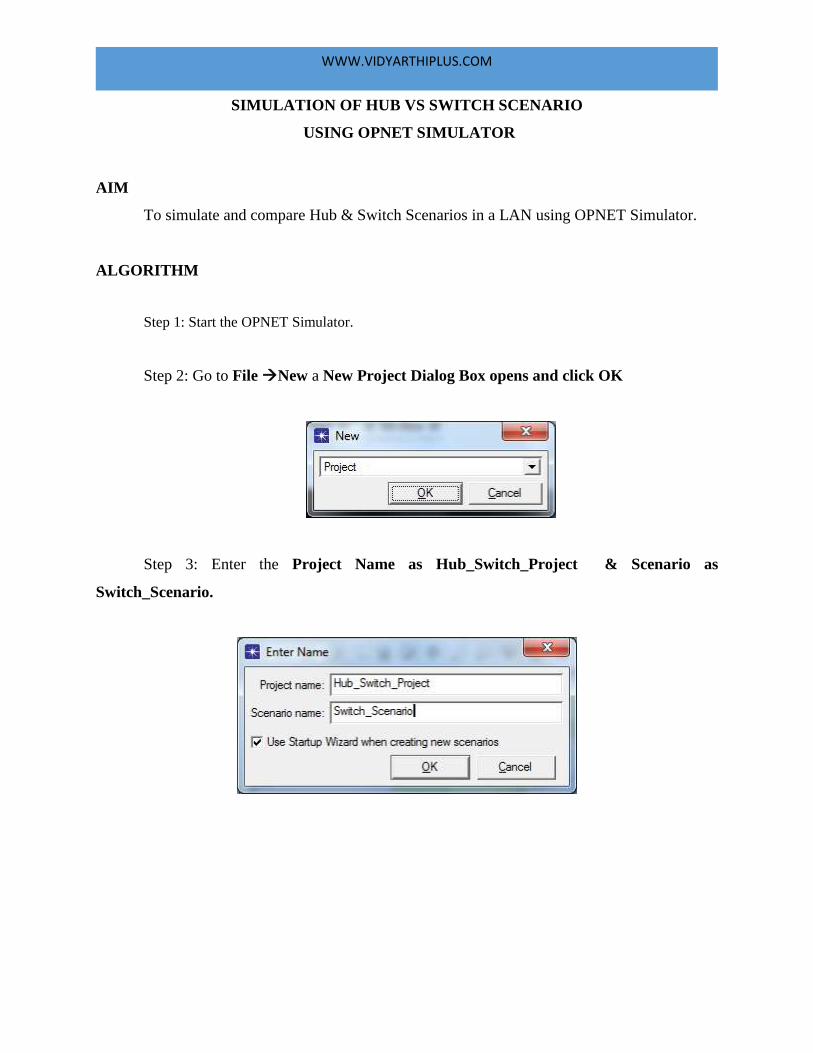
Step 2: Go to File New a New Project Dialog Box opens and click OK

Step 3: Enter the Project Name as Hub_Switch_Project & Scenario as

Switch_Scenario.


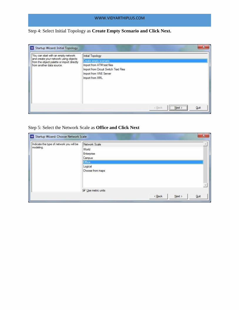
Step 4: Select Initial Topology as Create Empty Scenario and Click Next.

Step 5: Select the Network Scale as Office and Click Next


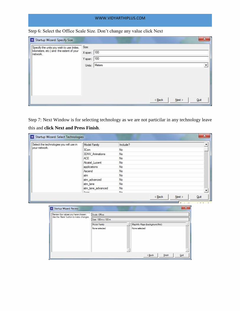
Step 6: Select the Office Scale Size. Don’t change any value click Next

Step 7: Next Window is for selecting technology as we are not particilar in any technology leave

this and click Next and Press Finish.


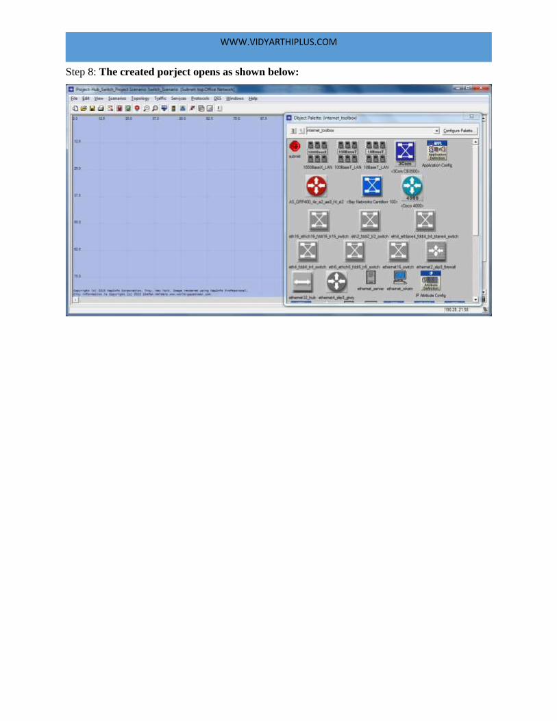
Step 8: The created porject opens as shown below:


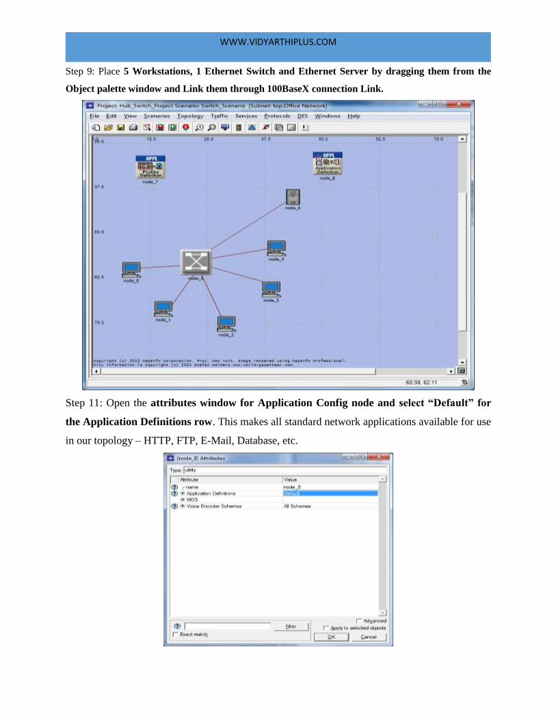
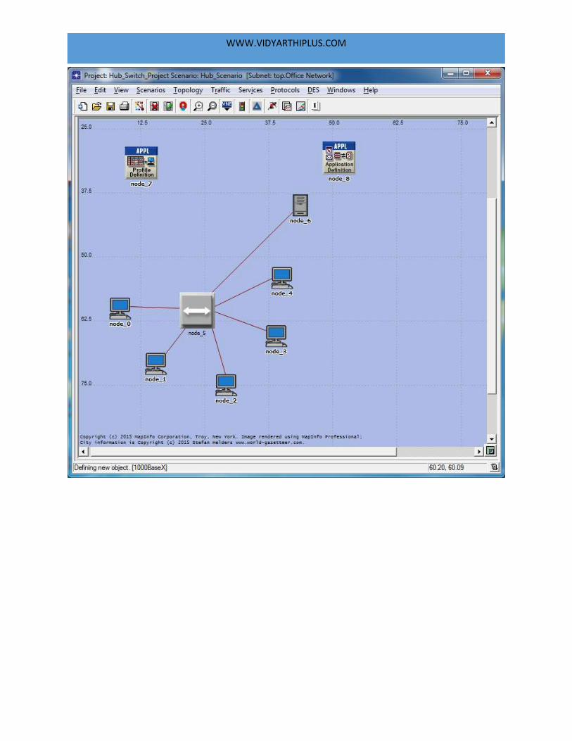
Step 9: Place 5 Workstations, 1 Ethernet Switch and Ethernet Server by dragging them from the

Object palette window and Link them through 100BaseX connection Link.

Step 11: Open the attributes window for Application Config node and select “Default” for

the Application Definitions row. This makes all standard network applications available for use

in our topology – HTTP, FTP, E-Mail, Database, etc.


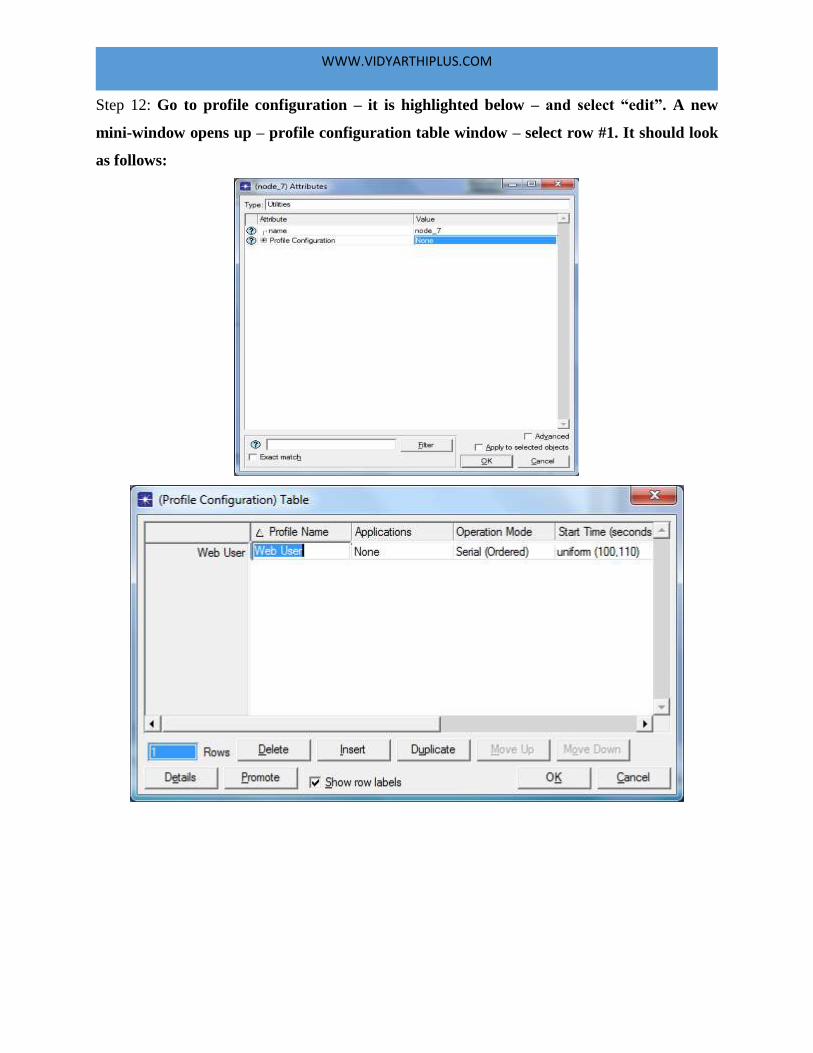
Step 12: Go to profile configuration – it is highlighted below – and select “edit”. A new

mini-window opens up – profile configuration table window – select row #1. It should look

as follows:


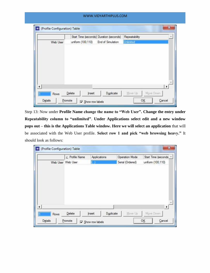
Step 13: Now under Profile Name change the name to “Web User”. Change the entry under

Repeatability column to “unlimited”. Under Applications select edit and a new window

pops out – this is the Applications Table window. Here we will select an application that will

be associated with the Web User profile. Select row 1 and pick “web browsing heavy.” It

should look as follows:


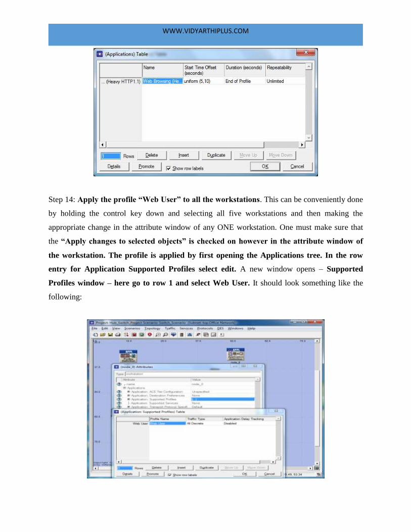
Step 14: Apply the profile “Web User” to all the workstations. This can be conveniently done

by holding the control key down and selecting all five workstations and then making the

appropriate change in the attribute window of any ONE workstation. One must make sure that

the “Apply changes to selected objects” is checked on however in the attribute window of

the workstation. The profile is applied by first opening the Applications tree. In the row

entry for Application Supported Profiles select edit. A new window opens – Supported

Profiles window – here go to row 1 and select Web User. It should look something like the

following:


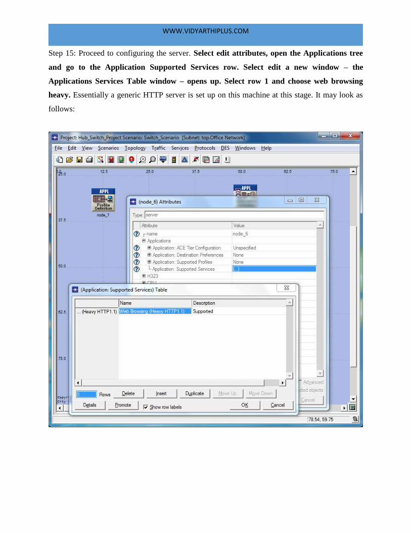
Step 15: Proceed to configuring the server. Select edit attributes, open the Applications tree

and go to the Application Supported Services row. Select edit a new window – the

Applications Services Table window – opens up. Select row 1 and choose web browsing

heavy. Essentially a generic HTTP server is set up on this machine at this stage. It may look as

follows:


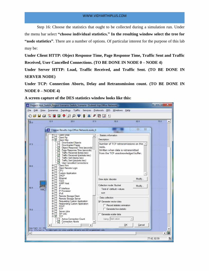
Step 16: Choose the statistics that ought to be collected during a simulation run. Under

the menu bar select “choose individual statistics.” In the resulting window select the tree for

“node statistics”. There are a number of options. Of particular interest for the purpose of this lab

may be:

Under Client HTTP: Object Response Time, Page Response Time, Traffic Sent and Traffic

Received, User Cancelled Connections. (TO BE DONE IN NODE 0 – NODE 4)

Under Server HTTP: Load, Traffic Received, and Traffic Sent. (TO BE DONE IN

SERVER NODE)

Under TCP: Connection Aborts, Delay and Retransmission count. (TO BE DONE IN

NODE 0 – NODE 4)

A screen capture of the DES statistics window looks like this:


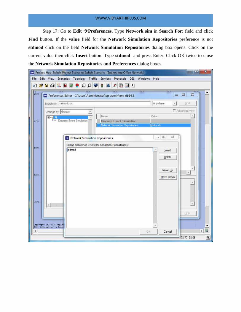
Step 17: Go to Edit Preferences. Type Network sim in Search For: field and click

Find button. If the value field for the Network Simulation Repositories preference is not

stdmod click on the field Network Simulation Repositories dialog box opens. Click on the

current value then click Insert button. Type stdmod and press Enter. Click OK twice to close

the Network Simulation Repositories and Preferences dialog boxes.


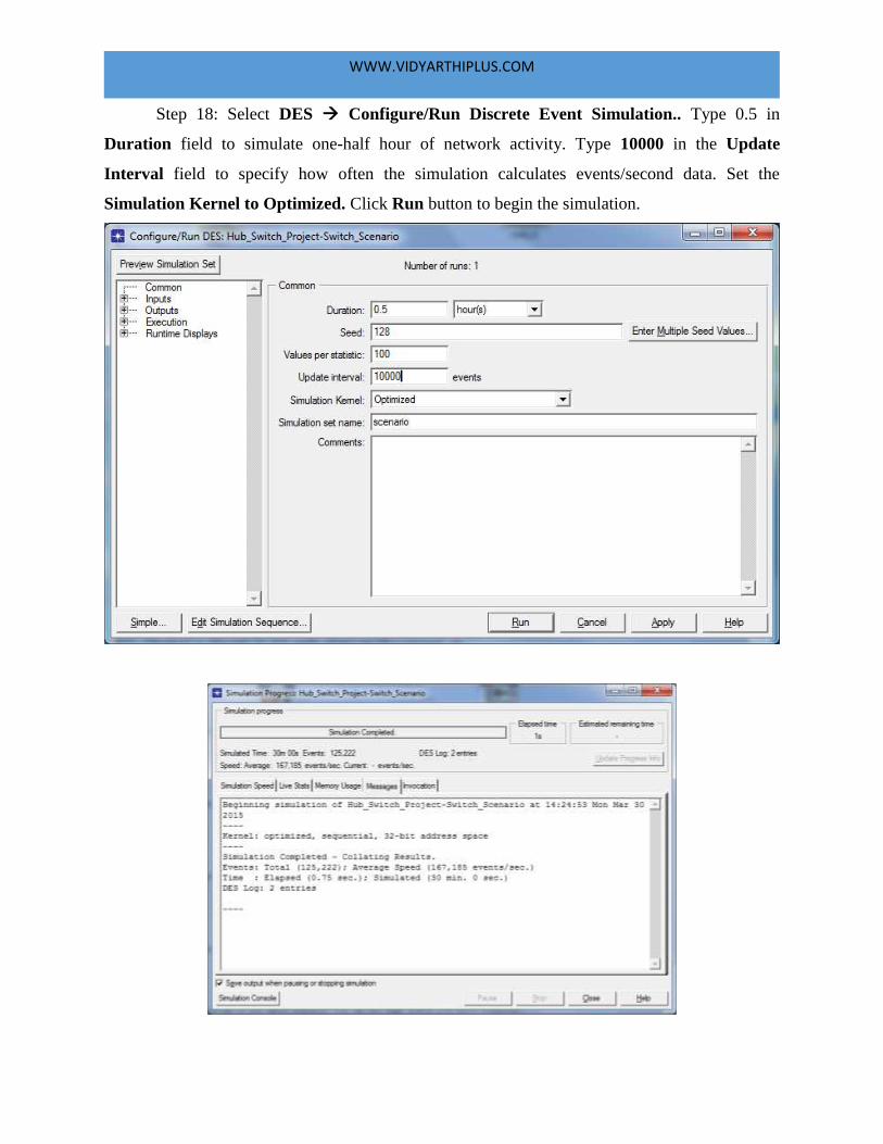
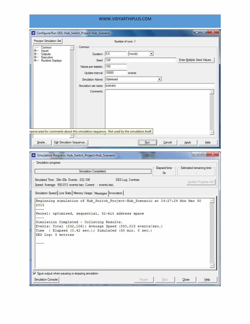
Step 18: Select DES Configure/Run Discrete Event Simulation.. Type 0.5 in

Duration field to simulate one-half hour of network activity. Type 10000 in the Update

Interval field to specify how often the simulation calculates events/second data. Set the

Simulation Kernel to Optimized. Click Run button to begin the simulation.


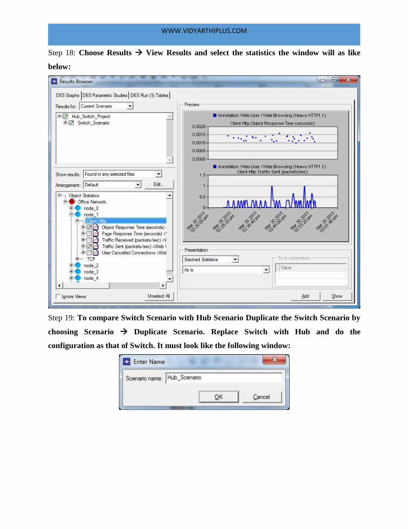
Step 18: Choose Results View Results and select the statistics the window will as like

below:

Step 19: To compare Switch Scenario with Hub Scenario Duplicate the Switch Scenario by

choosing Scenario Duplicate Scenario. Replace Switch with Hub and do the

configuration as that of Switch. It must look like the following window:


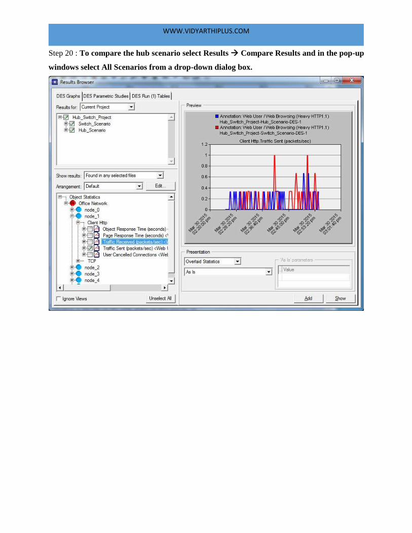
Step 20 : To compare the hub scenario select Results Compare Results and in the pop-up

windows select All Scenarios from a drop-down dialog box.


SIMUALTION OF OSPF USING OPNET SIMULATOR

AIM

To simulate OSPF protocol using ONET Simulator.

OPEN SHORTEST PATH FIRST PROTOCOL

The Open Shortest Path First (OSPF) protocol is an interior gateway protocol (IGP) used

for routing in Internet Protocol (IP) networks. As a link state routing protocol, OSPF is more

robust against network topology changes than distance vector protocols such as RIP, IGRP, and

EIGRP. OSPF can be used to build large scale networks consisting of hundreds or thousands of

routers.

Open Shortest Path First (OSPF) uses the Dijkstra’s algorithm to compute the shortest

path to a destination. The algorithm calculates the shortest path to each destination based on the

cumulative cost required to reach that destination. The cumulative cost is a function of the cost

of the various interfaces needed to be traversed in order to reach that destination.

The cost (or the metric) of an interface in OSPF is an indication of the overhead required

to send packets across that interface. The cost of an interface is calculated based on the

bandwidth -- it is inversely proportional to the bandwidth of that specific interface (i.e., a higher

bandwidth indicates a lower cost). For example, the cost of a T1 interface is much higher than

the cost of a 100Mbit Ethernet interface because there is more overhead (e.g., time delays)

involved in crossing a T1 interface.

Characteristic features of OSPF

Link State Based

Runs directly over IP

Interior or border gateway protocol

Multiple paths to each destination. Load balancing.

Link-attribute based costing. Costing is statically assigned.


PROCEDURE TO SIMULATE OSPF

1. Create a Network:

Step 1: Start OPNET and create a new project. File New… and choose Project.

Step 2: Name the project <initials>_OSPF and the scenario NoAreas. Click OK.

Step 3: Select Create empty scenario and click next.

Step 4: Select Office and click next.

Step 5: Set X Span to 200 and Y Span to 200. Click next.

Step 6: Do not include any technologies and click next.

Step 7: Review the values and click OK.

Step 8: Open the Object palette and change the palette to routers.

Step 9: Click OK.

Step 10: Place ten slip8_gtwy’s in the workspace.

Step 11: Change the object palette to internet_toolbox.

Step 12: Connect all the routers using PPP_DS3 link.

Step 13: Rename all the routers. Right click on each router and

select Set Name from the pop-up menu.

2. Configure Router Interface:

Step 1: Open the Protocols IP Routing Configure Routing Protocols… menu.

Step 2: Check the OSPF check box.

Step 3: Select the All interfaces radio button.

Step 4: Save the project.

3. Assign addresses to the router interfaces:

The Protocols IP Addressing Auto-Assign IP Addresses operation

assigns a unique IP address to the connected IP interfaces whose IP address is currently

set to auto assigned. This operation does not change the value of manually set IP

addresses.

The message Assigns 40 IP addresses appear in the status bar.


4. Configure Routing Cost:

Step 1: to change the interface cost across all interfaces, then, rather than individually

setting them on each interface, one can use the model-wide cost configuration option

using the following menu option:

Protocols OSPF Configure Interface Cost. This operation will allow for

choosing one of the following two cost configuration options:

i. The Reference Bandwidth will be set for all routers. All interfaces will be set

with a cost value of Auto Calculate.

ii. All interfaces will be set with the specified cost value. The interface/bandwidth

settings will be ignored.

Step 2: Select the links between:

Router A Router B

Router B Router D

Router D Router C

Router C Router A

Router B Router C

by shift clicking on them.

Step 3: Open the Configure Interface Metric Information dialog. Protocols IP

Routing Configure Interface Metric Information.

Step 4: Set the Bandwidth value to 5000 kbps.

Step 5: Select Interfaces across selected links radio button. Click OK.


Router B Router E

Router E Router G

Router I Router F

Router F Router D

Router E Router F








Router G Router H

Router H Router J

Router J Router I

Router I Router G

Router G Router J







5. Configure Traffic Demands:

Step 1: Select both Router B and Router D by shift clicking on them.

Step 2: Open the Create traffic demands menu. Protocols IP Demands

Create Traffic Demands…

Step 3: Select From Router B radio button.

Step 4: Click Create.

Step 5: Select both Router C and Router J by shift clicking on them.

Step 6: Open the Create traffic demands menu. Traffic Create Traffic Demand

IP Unicast.

Step 7: Select From Router C radio button.

Step 8: Click Create.

The paths of the traffic demands are now visible. To hide them select View Demand

Objects Hide All.


6. Configure Simulation:

Step 1: Open the Configure Discrete Event Simulation dialog.

Step 2: Set duration to 10 minutes.

Step 3: Click OK.


7. Duplicate Scenario:

Areas scenario

The major addition in OSPF configuration, relative to other protocols, is that the OSPF

routing domain can be divided into smaller segments called areas. This reduces memory and

computational load on the routers. Each area is numbered and there must always be an area zero,

which is the backbone. All other areas attach to the backbone either directly or via virtual

links. An area should contain no more than about 50-100 routers for optimum performance. A

router that connects to more than one area is called an Area Border Router (ABR).

1. Duplicate the scenario. Scenarios Duplicate scenario…

2. Name the scenario Areas.

Partition the network into areas. This is a physical partitioning in the sense that an

interface can belong to only one area. The distinct interfaces of the same router may still Belong

to separate areas.

3. Select the links between:

Router A Router B

Router B Router D

Router D Router C

Router C Router A

Router B Router C


4. Open the OSPF Area Configuration dialog. Protocols OSPF Configure

Areas.

5. Set the value 1 to Area Identifier.

6. Click OK.



Router B Router E

Router E Router G

Router I Router F

Router F Router D

Router E Router F



Areas.


10. Click OK.


Router G Router H

Router H Router J

Router J Router I

Router I Router G

Router G Router J



Areas.


14. Click OK.

15. Visualize the areas. Protocols OSPF Visualize Areas…

16. Click OK in the pop-up dialog.

17. Save the project.

The areas are visualized in different colors.


Balanced Scenario

Load balancing is a concept that allows a router to take advantage of multiple best paths

(routes) to a given destination. If two routes to the same destination have the same cost, the

traffic will be distributed half to each.

1. Go back to the NoAreas scenario. Scenarios Switch To Scenario NoAreas.

2. Duplicate the scenario. Scenarios Duplicate scenario…

3. Name the scenario Balanced.

4. Select both Router C and Router J by shit clicking on them.

5. Open the Configure Load Balancing Option dialog. Protocols IP Routing

Configure Load Balancing Option.

6. Select Packet based in the roll-down menu.

7. Select the Selected Routers radio button.

8. Click OK.

9. Save the project.

8. Run the simulation

1. Open the Manage Scenarios dialog. Scenarios Manage Scenarios…

2. Click in the Results column on the NoAreas row and click the collect button.

3. Set the scenarios Area and Balanced to collect results. Repeat the previous step.

4. Click OK to run the simulation.

5. Click Close when the simulation has finished.

9. View the results:

NoAreas scenario

1. Switch to the NoAreas scenario. Scenarios Switch to Scenario NoAreas.

2. Open the Route Report for IP Traffic Flows dialog. Protocols IP Demands

Display Routes for Configured Demands…

3. Expand Sources Router B Router D.

4. Select Router B Router D.

5. Change the Display attribute to Yes.

6. Change the Display attribute for Router B Router D to No.


7. Expand Sources Router C Router J.

8. Select Router C Router J.


Areas scenario

1. Switch to the Areas scenario. Scenarios Switch to Scenario Areas.



3. Expand Sources Router B Router D.

4. Select Router B Router D.


Balanced scenario

1. Switch to the Balanced Scenario. Scenarios Switch to Scenario Balanced.



3. Expand Sources Router C Router J.

4. Select Router C Router J.


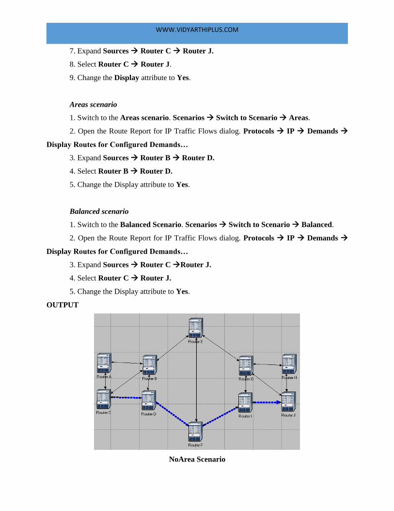
OUTPUT

NoArea Scenario


Area Scenario

Balanced Scenario

simulation of hub vs switch scenario using opnet …

Documents