Simulation of Energy Storage Tanks

with Surface Heat Exchangers

by

Jrg Michael Baur

A thesis submitted in partial fulfillment of

the requirements for the degree of

Master of Science

(Mechanical Engineering)

at the

University of Wisconsin Madison

1992

Abstract

Cold climate protection for solar domestic hot water systems is usually

implemented using an antifreeze solution in the collectors with heat

exchange to water in the storage tank. The heat exchanger can be external or

internal to the tank. The different types of internal heat exchangers can be

classified as internal coil, wrap-around heat exchange wall or mantle heat

exchanger. This paper investigates the performance of a mantle heat

exchanger. A mantle heated water storage tank is a cylindrical storage tank

surrounded by an annulus. The hot liquid from the collector flows through

the annulus (mantle) and transfers energy to the contents of the tank. The

separating wall is the heat exchange surface. An advantage of this design is

the reduced system complexity achieved by combining the heat exchanger and

the storage unit into one element. In addition flow in the tank occurs only

when water is delivered to the load, resulting in better temperature

stratification compared to tanks using external heat exchangers. Regarding

temperature stratification tanks with mantle heat exchangers are also better

than coil in tank systems as the heat input to the tank is spread over a much

wider vertical range. A high degree of stratification is desirable because it

increases the useful output of the collector by supplying it with colder water.

ii

Mantle heat exchangers are limited to small scale solar hot water systems

because the mantle heat transfer area to volume ratio decreases with

increasing storage capacity.

A numerical model of the heat exchanger was written as a subroutine

(type) for TRNSYS, the transient system simulation program. The tank is split

into a user-specified number of horizontal layers each with a uniform

temperature. The energy transferred to or from a node includes mass flow

due to the load, heat exchange with the environment, heat transfer from the

fluid in the mantle, and conduction between the layers. Classic correlations

are used to determine heat transfer coefficients. The energy balances lead to a

set of differential equations which are solved iteratively.

The program is tested by comparing simulation results with experimental

data. In order for the model and experiments to agree it is necessary to modify

the heat transfer coefficients on the inside of the tank and in the mantle with

a correction factor. The results of a parametric study to find the impact of

different factors on the solar fraction of a complete solar domestic hot water

system is presented.

iii

I

Acknowledgments

Not only to my own surprise the ceuvre really is completed. Even though

anthropomorphic computers turned the letters of the newly written last

chapter irreversibly into little pictures and Arabic letters, crashed just in time

before the imminent autosave and in two out of three cases refused to read

the valuable contents of my diskettes - I reached the goal.

I want to thank Sandy for giving me valuable hints for my research and

for taking time to help me when I got stuck, even during times when he was

extremely busy. I also want to thank Bill, my second adviser during the last

semester, who helped me finding some inconsistencies in my work. Special

thanks go to Osama and Prof. Dave Otis who helped me to bring some light

into the jungle of free convection in hot water tanks.

This thesis would have been completely impossible without the exchange

program of the Institut f ir Werkzeugmaschinen and the German Academic

Exchange Service (DAAD). I thank them for organizing the program and for

funding me during the first nine month. During summer and fall 1992 I was

funded by the Department of Energy as a research assistant. Thank you for that

opportunity.

iv

r

My research would have been meaningless without the experimental data

I got from Thermal Insulation Laboratory in Denmark and from the Solar

Calorimeter Laboratory in Denmark. Thanks to Simon Furbo for immediately

answering my requests and thanks to Prof. Steve Harrison and Brian Weir for

taking the experimental tank apart and providing me with the information

needed.

Many thanks to my office mates Jiirgen, Oystein, Bernd, Dick, Doug, Jeff,

Todd, Emily and Tim who helped me with infinite patience and expertise in

the sometimes desperate battle against the computers. I also want to thank all

the nice people who were in the Solar Lab with me for the enjoyable time.

I had a wonderful time in Madison and I want to thank all my friends and

my roommates for making my stay a great experience. I will miss Madison

and its friendly inhabitants very much.

v

Table of Contents

Abstract. i

Table of Contents . vi

N om enclature,................................................................................ x

1. Introduction .. ..... 1

2. Background .................................................................... 32. 1 Differences between Conventional Systems and Surface

Heat Exchanger Tanks.............................. 3

2. 1. 1 D escription ......................................................................... 3

2. 1. 2 Advantages of Thermal Stratification.................... 5

2. 2. Different Tank Designs.............................7

2. 3. A spects of M odeling ....................................................................... 9

vi

2.3.1. Design of a model................................ 9

2. 3.2. TRNSYS.................................................................................. 9

2. 4. Previous Approaches .......................................................................... 10

3. Description of Models..............................12

3. 1. Modeling Assumptions.............................12

3. 1. 1. Discretization of Time ..................................................... 13

3. 1. 2. Storage Tank ............................... 13

3. 1. 3. Mantle...................................14

3. 1.4. Heat Transfer Coeffi cient ................................................. 15

3. 1. 5. Temperature Inversions ................................................ 16

3. 1. 6. Conduction between Nodes.......................... 17

3. 2. Mathematical Description...........................17

3.2.1. Tank Nodes............................................................ 17

3. 2. 2. Mantle Nodes with Quasi Steady State Model........21

3. 2. 3. Mantle Nodes with Transient Model.................... 24

3. 2. 4. Heat Transfer Coefficient ... .................. 27

3. 2.5. Temperature Inversions......................29

3. 2. 6. Conduction between Nodes...................30

3. 3. Discussion of Chosen Assumptions................ ............ 31

3.3. 1. Mantle Nodes ............. ........ ............ 31

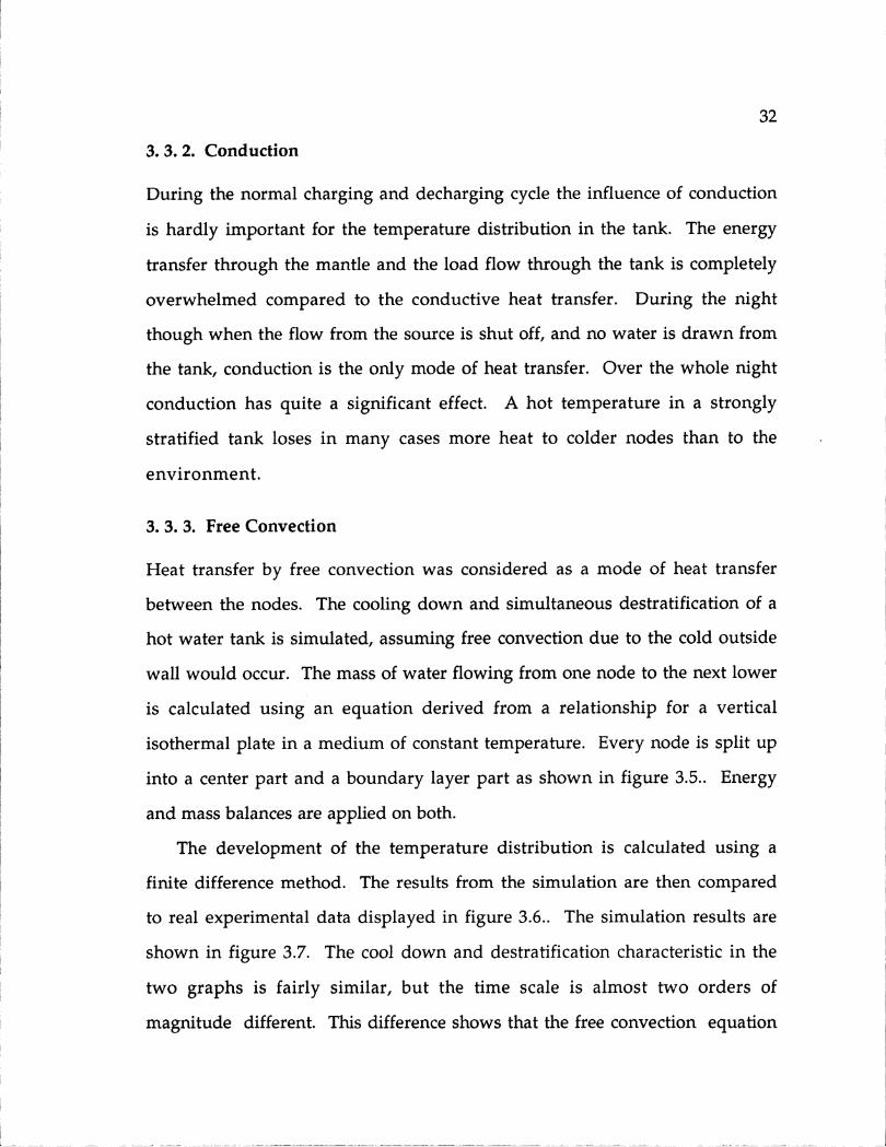
3. 3. 2. Conduction........................ ..... ............... 32

3. 3. 3. Free Convection...... ................. .......................32

3. 4. Algorithm................................................................... 35

vii

4. Verification of Model 38

4. 1. Testing of a Model................................38

4. 2. Experiments with Low Collector Flow Rates....................40

4. 2. 1. Heating Experim ent ........................................................ .43

4. 2. 1. 1. Description of Experiment ................ 43

4. 2. 1. 2. Simulation Results for Model I...............45

4. 2. 1.3. Simulation Results for Model II.............49

4. 2. 1. 4. Comparing Simulation Results from

Model I and Model II...................51

4. 2. 2. Experiment with Draws ................................................ 52

4. 2. 2. 1. Description of Experimental Set Up...........52

4. 2. 2. 2. Simulation Results from Model I.............52

4. 2. 2. 3. Simulation Results from Model II...........57

4. 2. 3. Cooling Experim ent ........................................................ 59

4. 2.3. 1. Description of Experiment ............ 59

4. 2. 3. 2. Simulation Results from Model I and

M odel II ................................................... 59

4. 3. Experiment with Regular Flow Rates..................62

4. 3. 1. Description of Experiment.........................62

4. 3. 2. Simulation Results with Model I.....................66

4. 3. 3. Simulation Results with Model II.....................70

5. Investigation of Mantle Heat Exchanger Tanks ............ 74

5. 1 Sample System............................................................. 74

5. 3. Variation of Parameters................................................. 76

viii

5. 3 . Mantle Heat Exchanger vs. System with Separate Heat

Exchanger .................................................... 78

6. Conclusion and Recommendations .... ................ 82

Appendix. ...... 84

Appendix A: TRNSYS Component Configuration...................84

Appendix B: Property Relations for Aqueous Propylene-Glycol ....... 88

Appendix C: TRNSYS-Decks............................89

Appendix D: FORTRAN Source Code .............................................. 97

References.110

ix

Nomenclature

Aenv common surface area of tank node and environment

Am common surface area of tank node and mantle

Ac cross sectional area of the mantle

At cross sectional area of the tank

C1 heat transfer correction factor on mantle side of heat exchanger

surface

cp specific heat of water in tank

Cp,af specific heat of anti freeze in collector loop

Dman diameter of mantle

Dtank diameter of inner tank

Dh hydraulic diameter of mantle (twice spacing)

enman distance to bottom of mantle from bottom of tank

hman distance to top of mantle from bottom of tank

k constant

kaf conductivity of anti freeze fluid in mantle

kst conductivity of steel walls

Li height of tank node i

m number of nodes in the mantle

x

mi mass of water in tank node i

rnH mass flow rate to and from heat source

rnjL mass flow rate to load

n number of nodes in the storage tank

Nui Nusselt number in node i

Nu(x) average Nusselt number from start of flow to x

p propylene glycol percentage anti freeze liquid in %

Pr Prandtle number

qcond heat transfer by conduction

Qload heat transfer caused by load flow

01oss heat transfer from tank or mantle to environment

Qman heat transfer from mantle to tank

Qtank heat transfer from mantle to tank

Re Reynolds number in mantle

Ri conduction resistance between node i and node i+1

t time

At length of time step

tw thickness of heat transfer surface

Tenv temperature of environment

Tm, avg average temperature over height of mantle nodes

Tm,in inlet temperature of mantle node

Tt i average temperature in tank node i

Tt, initial temperature in tank node at beginning of time step

Tt, final temperature in tank node at end of time step

Tt, avg average temperature in tank node during time step

xi

Tw weighted average temperature of environment and tank node

Ut-env loss coefficient from tank to environment

Ut-m heat transfer coefficient from tank to mantle

Um-env loss coefficient from mantle to environment

V tank volume

Xi length from mantle inlet to end of ith node

Axi distance between center of node i and node i+1

Greek letters

m viscosity of anti-freeze liquid in mantle

p density of fluid in tank

xii

1. Introduction

A major concern of current research in solar thermal processes is to improve

the efficiency and consequently the feasibility of existing systems. Simulations

are a tool for investigations in these areas because they allow the user to

obtain rapid system performance estimates without running expensive

experiments.

The two most important components of thermal solar systems for

domestic applications are the solar collector and the heat storage unit. The

object of this thesis is to describe a modeling approach for a sensible hot water

storage tank with a built in heat exchanger. The investigated tank is

cylindrical with an annulus (or mantle) around it. The hot liquid coming

from the collector flows through the mantle and transfers energy to the

contents of the tank. The separating wall is used as the heat exchanger surface.

This concept is an interesting alternative to conventional tanks with a

separate heat exchanger unit. One advantage of the surface heat exchanger

storage tanks is that it reduces the complexity of the system by combining the

heat exchanger and the storage unit in one element. The main difference

compared to the conventional tank is that the flow from the heat source does

not go through the tank so that the load flows through the tank in a less

2

disturbed manner. The effect is reduced turbulence and, as a result, better

temperature stratification. High stratification is desirable because it increases

the efficiency of the solar system. The efficiency increases because the water

returned to the collector is colder than in tanks with a more homogeneous

temperature distribution which reduces the thermal losses of the collector.

In Chapter 2 three different designs of hot water storage tanks with built in

surface heat exchangers are introduced. They are compared to conventional

systems with external heat exchangers. The procedure and design goals of

simulation software is discussed. This particular code is written as a

subroutine for the TRaNsient SYstem Simulation program (TRNSYS).

Consequently a summary of TRNSYS is included. Two different modeling

approaches for this kind of sensible heat storage exist already and are

investigated at the end of this chapter.

Different collector flow rates make different modeling assumptions

necessary. The two different models used are described in Chapter 3. For high

collector flow rates (i. e. mantle flow rates) the flow through the mantle is

assumed to be in a quasi-steady state during the whole time step. For low flow

systems, the energy stored in the mantle has to be included as it can be a

significant part of the total energy stored.

To validate the model, simulations of real test situations have been

performed. The procedure of the experiments is described in chapter 4. The

results are compared to the real experiments, and deviations are discussed.

The surface heat exchanger tank model is used in chapter 5 to compare

this kind of storage component to the conventional system. The impact the

stratification has on the performance of the system is also investigated.

3

2. Background

2. 1 Differences between Conventional Systems and Surface Heat

Exchanger Tanks

2. 1. 1 Description

In most climates in the United States and in Europe, freezing conditions occur

regularly. To avoid damage to exposed system components like piping and

the solar collector, an anti-freeze liquid is run through the collector. The anti-

freeze liquid has to be separated from the water used in the house by a heat

exchanger. The heat exchanger can be located either on the collector side (i. e.

water is stored in the tank) or on the load side (i. e. anti-freeze liquid is stored)

of the sensible heat store. In most designs the first option is chosen because it

reduces the necessary amount of anti-freeze liquid. Furthermore, the draw

rate is less restricted because the load flow doesn't have to run through a heat

exchanger with a limited heat transfer capacity.

The main difference between the conventional system and the surface

heat exchanger tank is the mode in which heat is transferred from the anti-

4

freeze liquid to the water stored in the tank. As displayed in figure 2.1 the

conventional system requires an additional intermediate loop between the

collector and the tank. In the conventional system water is drawn out from

the bottom of the tank (using an extra pump), heats it up in a separate heat

exchanger and fills the heated water back in the top of the tank. The locations

of the inlets and outlets are chosen according to the temperature profile,

which is hotter at the top and colder at the bottom of the tank. This method

creates an additional flow through the tank which is unnecessary when a

surface heat exchanger is used. This design allows the hot anti-freeze to run

directly over the side wall of the tank in a containment surrounding the tank.

The contents of the tank are directly heated from the top to the bottom. As the

load flow is upwards, the tank acts as a counterflow heat exchanger. The

mantle typically covers the lower three quarters of the tank height (except in

the tank-in-tank design, compare chapter 2. 2). The mantle has to start at the

bottom otherwise the volume below the mantle could not be used for heat

storage.

System with Mantle Heat Exchanger Conventional System with Separate

Collector Loop

Figure 2.1: Comparison of Systems

5

A big advantage of the tank with a surface heat exchanger is, that it

significantly reduces the complexity of the system. The system consists of one

less separate heat exchanger, which not only saves space but it also saves the

four attachments at the heat exchanger, two pipes a pump and depending on

the design a controller. Even though the tank with the surface heat exchanger

is more expensive than a regular tank, the overall system may be substantially

cheaper. Also the pumping costs are slightly reduced as the pressure drop is

not as high as in a conventional heat exchanger.

The most important advantage, however, is improved thermal

stratification in the surface heat exchanger tank. This effect was seen by

Fanney and Klein [2] who performed yearly experiments comparing different

solar systems. The improved stratification is due to a reduction in mixing

since only the load flow goes through the tank instead of two flows in the

opposite direction as it is the case in conventional systems. The advantages of

a good thermal stratification are described in the next section.

The application of surface heat exchanger tanks is generally limited to

domestic hot water systems as the effectiveness of this kind of heat exchangers

declines with growing volumes. This behavior occurs as the mantle area to

volume ratio decreases with increasing storage capacity.

2. 1. 2 Advantages of Thermal Stratification

Thermal stratification is a temperature distribution where the top of the tank

is at the highest temperature and decreases gradually down the tank. The

reason for this effect is that the density of hotter water is lower than of cooler

water.

6

All solar thermal storage tanks exhibit some degree of stratification but to

illustrate the effect of high stratification in a tank, it is compared to a fully

mixed tank. In a stratified tank the bottom of the tank is colder than in a fully

mixed tank therefore the water fed into the collector is colder. The colder the

liquid going into the collector, the higher is the efficiency of the collector. The

reason for that is that the losses are reduced. The losses are proportional to

the difference between the average liquid temperature in the collector and the

ambient temperature. Therefore low insulated collectors like collectors with

single or no glazing have the biggest benefits from the low stratification.

Stratified Tank Fully Mixed Tank

I I

60oC I40o I

500 °C40 °C400 I40C

300C I 40 IC

20 0° I 40O C I

35 00 350°C

Figure 2.2: Increased Useful Energy due to Stratification

Stratification not only increases the collector efficiency, it also increases the

storage effectiveness under certain conditions. For example consider the

situation in figure 2.2: A highly stratified and a fully mixed tank contain the

same energy. If the critical temperature is, for example, 35 0C the useful

energy is proportional to the area to the right of the critical temperature line.

7

This useful energy or utilizability [5] is 1. 8 times higher in the stratified tank

compared to the fully mixed tank.

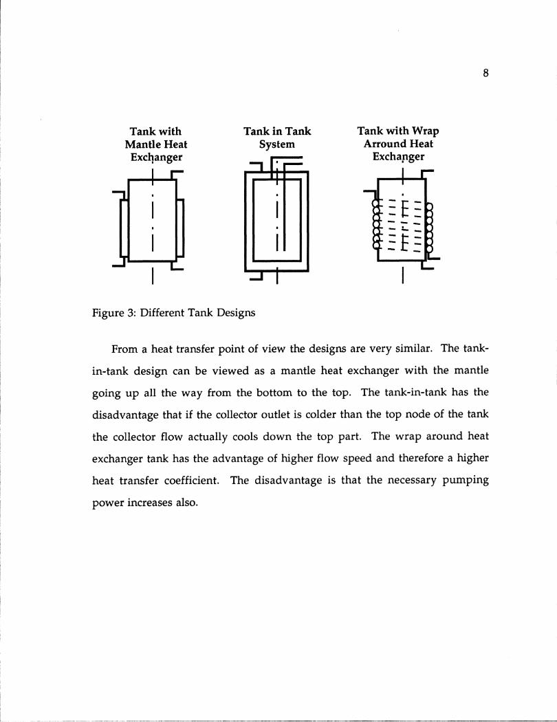
2. 2. Different Tank Designs

The model must consider the various designs for tanks with built in heat

exchangers which perform slightly different. One design is an immersed coil

inside of the tank. It is not examined here, because it does not maintain

stratification very good. The three most common types of tanks with surface

heat exchanger are displayed in Figure 3.

A mantle heat exchanger is an annulus shaped cylinder around the wall of

the tank. The mantle starts slightly above the bottom and goes up to

approximately three quarters of the height of the tank. The tank-in-tank

system is a containment which is completely immersed in a bigger tank

through which the collector flow runs. In the third design a coil is wrapped

around the side wall and welded to it.

As all three of these designs are not very common it is hard to say which

one is the most economical. It is very likely that the tank-in-tank system can

be produced pretty inexpensively using, for example, plastic as material for the

outer tank. The most expensive design seems to be the tank with the coil

welded to it as it is the most labor intensive design. Although there is a

method called roll bonding where two sheets of metal are bonded together in

some areas. The not bonded area is in the form of a spiral like the coil in the

classic method. The not bonded area is then filled with water or air and

pressurized to form a coil like shape.

Tank withMantle HeatExchanger

Tank in TankSystem

Tank with WrapArround Heat

Exchanger

Figure 3: Different Tank Designs

From a heat transfer point of view the designs are very similar. The tank-

in-tank design can be viewed as a mantle heat exchanger with the mantle

going up all the way from the bottom to the top. The tank-in-tank has the

disadvantage that if the collector outlet is colder than the top node of the tank

the collector flow actually cools down the top part. The wrap around heat

exchanger tank has the advantage of higher flow speed and therefore a higher

heat transfer coefficient. The disadvantage is that the necessary pumping

power increases also.

8

2. 3. Aspects of Modeling

2. 3. 1. Design of a model

Before a computer program can be written, the thermal behavior in the tank

has to be approximated by a model. The model can never take into account all

the phenomena that actually occur. Therefore the required exactness of the

model depends very much on the application. If the flow pattern in the tank

is of importance or an equation to calculate the Nusselt number is to be

developed a finite element approach with a fine mesh would be appropriate.

In that case the computation would take many times longer than an

experiment. If only a fast and very rough estimate is required maybe a simple

energy balance at a fully mixed tank would be sufficient. This kind of

approach lacks the ability to distinguish between different designs. In essence

the problem is to find the right tradeoff between numerical exactness and

computation speed. In this case the requirement for the exactness is that the

model should show the distinctive behavior of the particular design and the

error should be in the same margins like in other designs. The required

computation time should be in the same order of magnitude like for other

components in TRNSYS. The implied subroutine leaves a big part of this

decision to the user as it allows him or her to choose the number of nodes in

which the tank is split up between one and fifteen.

2. 3. 2. TRNSYS

The simulation code for the surface heat exchanger tank was written as a

subroutine for the TRaNsient SYstem Simulation program (TRNSYS [4]).

TRNSYS is capable of predicting the performances of several kinds of energy

10

systems like active and passive solar thermal energy systems, photovoltaic

systems, solar cooling systems, air conditioning systems, and refrigeration

systems. The diversity of the program is achieved by allowing the user to

simulate a certain system by combining different TRNSYS components. The

user specifies the system setup in a TRNSYS-deck. The main TRNSYS

routine then calls the different components in form of subroutines. The

program then calculates the temperatures and other transient values for every

time step by iterating until the changes are within the specified tolerances.

2.4. Previous Approaches

Today, there exist two simulation programs for surface heat exchanger tanks.

The concepts behind these two models are quite different. The model by

Furbo [1] of the Thermal Insulation Laboratory at the Technical University of

Denmark uses a finite difference method. The model used in WATSUN [6],

which is a solar energy simulation program by the WATSUN Simulation

Laboratory at the University of Waterloo in Ontario, Canada uses heat

exchanger equations.

In the Danish program the water in the tank, the water in the mantle, and

the steel walls of the tank are divided into elements. The temperatures in

these nodes are evaluated by an implicit finite difference formulation. The

energy balances used include only thermal conduction. Flow streams are

accounted for by exchanging entire control volumes. If a temperature

inversion occurs, the affected nodes are mixed. Heat (or liquid) transfer by free

convection is considered to be negligible. The heat transfer coefficient from

11

the mantle liquid to the heat exchanger surface and the heat transfer

coefficient from that surface to the liquid in the tank are equal. These

coefficients were obtained by a linear curve fit to experimental data. This

method leads to a relatively high computational effort and is therefore not

appropriate for the use in TRNSYS. The heat transfer coefficients used during

charging periods (ranging from 550 to 200 W/m 2 K from mantle inlet to

outlet) were found to be roughly three times greater than the values obtained

when equations for laminar flow between parallel plates with one side

insulated [5] were used.

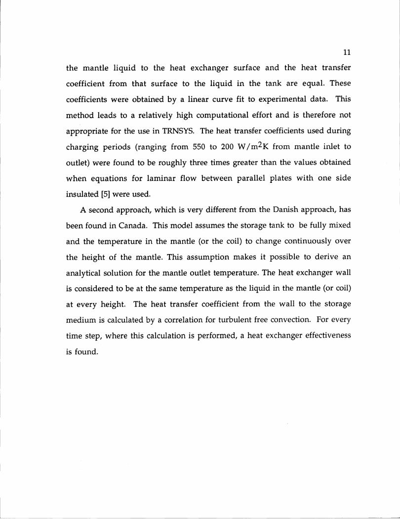
A second approach, which is very different from the Danish approach, has

been found in Canada. This model assumes the storage tank to be fully mixed

and the temperature in the mantle (or the coil) to change continuously over

the height of the mantle. This assumption makes it possible to derive an

analytical solution for the mantle outlet temperature. The heat exchanger wall

is considered to be at the same temperature as the liquid in the mantle (or coil)

at every height. The heat transfer coefficient from the wall to the storage

medium is calculated by a correlation for turbulent free convection. For every

time step, where this calculation is performed, a heat exchanger effectiveness

is found.

12

3. Description of Models

3. 1. Modeling Assumptions

To account for the fact that different users have different needs related to the

tradeoff between exactness and computational effort (compare chapter 2.3.1),

the user is offered multiple options. The user has the choice of splitting the

tank up into any number of nodes between one and fifteen. More important

though, one has the choice between two models. The first model treats the

liquid in the mantle as a volume of liquid, where the temperature of the

liquid changes gradually over the height of the mantle, but is constant over

the time step. This means that during a time step, the flow through the

mantle can be assumed to be at steady state. In the second approach, the

mantle is divided into fully mixed control volumes to which energy balances

are applied to account for the energy change in the mantle during that

particular time step. Model I is also referred to as quasi steady state model

while model II is referred to as a model including mantle energy storage.

13

3. 1. 1. Discretization of Time

When simulating any kind of transient behavior there are two ways to take

care of the time influence. Occasionally it is possible to derive an analytical

solution, where the equations depend directly on the time. However, in most

cases, especially with variable input values, the only possibility is to solve the

differential equations numerically using discrete time steps. In the latter case

the derivative of a variable is approximated by using the difference of their

present value and their value from the time step before, divided by the length

of a time step. The referenced models use a combination of the two methods.

Time is discretized in time steps so that the changing input values can be

taken care of. The temperature at the end of a time step in a tank node is

evaluated using an analytical equation. The calculation starts with the

respective initial temperature. For the heat transfer calculations an average

temperature is determined. This average temperature results in the same

amount of heat transfer that the changing temperature would have caused.

3. 1. 2. Storage Tank

The size and shape of the control volumes, which both have to be good

approximations of the real three-dimensional temperature distribution in the

tank, affect the performance of the simulation the most. In both models the

liquid in the main tank is split up into horizontal layers. Temperature

changes over the radius are thus neglected. This configuration reflects the

physical occurring thermal temperature layers whereas it neglects the

influence of the fluid being hotter at the heat transfer surface than in the

middle of the nodes The convective flow of the load and the heat transferred

from the mantle and to the environment change the temperature in the

14

entire control volume permanently, as the liquid in the control volume is

fully mixed at every point in time. In Figure 3. 1. it is shown how a tank could

be designed to behave exactly like the model. Between the tank nodes

divisions are located and the liquid in each section is always fully mixed by a

fan.

Figure 3. 1.: Illustration of Tank Model

3. 1. 3. Mantle

The mantle is split up into horizontal layers, matching the nodes in the tank

so that the average tank node temperature can be used to calculate the heat

transfer from the mantle. The determination of the temperature distribution

depends on the mass flow rate through the collector. For high flow rates,

model I is used, and the flow in the mantle is considered to be at steady state

during the time step. The temperature in the mantle nodes are assumed to

c: o

mm

mmm

15

change gradually, usually to cool down as it flows down. In every mantle

node an equivalent temperature is determined, which results in the same

heat transfer as the existing temperature distribution in the mantle node

would cause. This equivalent temperature is calculated using the inlet

temperature in the node and by assuming that both the temperature of the

environment and the temperature of the tank node do not vary over the

height of the tank node. The inlet temperature of the top node is the inlet

temperature to the mantle and the inlet temperatures of the lower nodes are

calculated like the average temperature from the inlet temperature of the

node above. Therefore the mantle node temperatures are calculated

sequentially from the top to the bottom.

In model II, the energy change in the mantle is taken into account by

applying the same kind of energy balance on the mantle nodes as it was used

for the tank nodes (compare to section 3.1.2.). The mantle nodes are

considered to be fully mixed and a temperature averaged over time is

determined. This average temperature is used for the heat transfer

calculations.

3. 1. 4. Heat Transfer Coefficient

For the model to perform well, it is important to use good estimates for

the heat transfer coefficient between the mantle and the tank. The previous

approaches (section 2. 4.) use completely different approaches. The WATSUNmodel for wrap-around heat exchangers neglects the resistance from the

mantle to the wall and uses heat transfer coefficients from a turbulent free

convection equation on the inside of the wall. In the TIL-model the heat

transfer coefficients are obtained by fitting them to experimental data.

16

The heat transfer from one fluid to the other through a wall splits up into

the heat transfer from the hotter fluid to the wall, the conduction through the

wall and the heat transfer from the wall to the colder fluid. The heat transfer

coefficient is the reciprocal value of the sum of the three resistances.

Comparing the orders of magnitude it turns out that the resistance for the

conduction through the wall can be neglected compared to the resistance from

the mantle to the wall. The resistance on the tank side of the wall can be

defined by setting the corresponding heat transfer coefficient to a constant

value in the TRNSYS deck. This resistance can be assumed to have only a

small influence on the overall heat transfer coefficient. Therefore it is

suggested to set this heat transfer coefficient to a high value in the TRNSYS

deck. The heat transfer from the mantle fluid to the wall is calculated with an

empirical equation for laminar flow between flat plates with one side

insulated and constant heat flux on the other side.

The heat loss coefficient to the environment is an input parameter to the

TRNSYS-deck. It is usually obtained by a cool down test.

3. 1. 5. Temperature Inversions

Liquids naturally stratify in a way so that the temperature of the fluid is

high at the top and gradually decreases towards the bottom as the density of

hot water is lower compared to cold water. Sometimes situations occur where

a control volume in the middle of the tank is hotter than a node at the top.

This situation occurs because in most cases the mantle does not extend to the

top of the tank, therefore middle nodes are heated, while the top nodes have

comparably high losses to the environment. A situation like this is unstable.

Therefore it is assumed that the hot water rises and mixes with the colder

17

water above. If the mixing temperature continues to be higher than the

temperature of the next node above, then this node is mixed in also.

3. 1. 6. Conduction between Nodes

Heat transfer by conduction between the nodes can be taken into account. The

heat is conducted two different ways. Heat is conducted directly from one

control volume of water to the next. The distance for the heat transfer is

chosen to be the distance between the centers of the two control volumes in

question. Apart from the direct heat transfer, energy is transferred from the

node to the tank wall, into the wall, and finally back to the next node.

3. 2. Mathematical Description

3. 2. 1. Tank Nodes

The equations used to determine the temperature in the tank and mantle

nodes are based on the first law of thermodynamics and the most basic heat

transfer equation. The first law of thermodynamics requires that the change

in enthalpy, which is proportional to the change in temperature in a fixed

mass of matter, is proportional to the rate of the net energy input in this mass

of matter. The heat transfer law says that the rate of energy transferred from

one medium to the other is proportional to the temperature difference

between the two media.

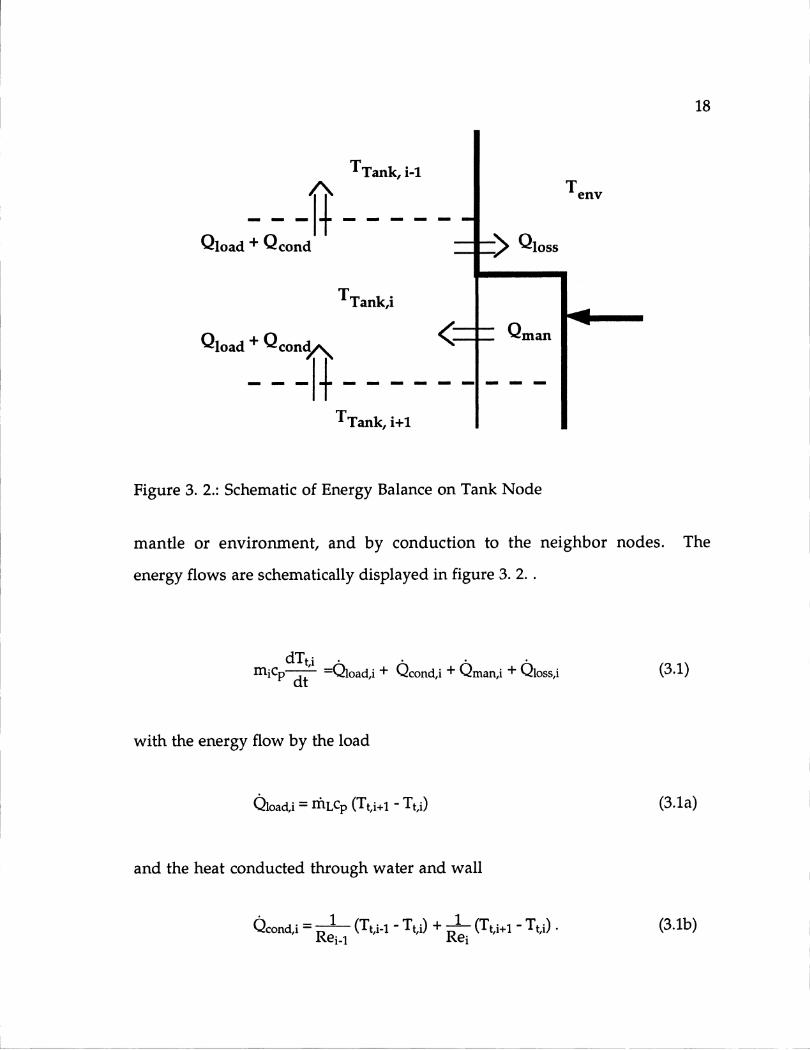
Equation (3.1) is the energy balance at a representative tank node

including the energy transferred by the load flow, by heat transfer to the

1

I

TTank, i-i

A

Qload + Qcond

TTank,i

Qload + Qcond

TTank, i+1

Tenv

_> Qloss

Qman

Figure 3. 2.: Schematic of Energy Balance on Tank Node

mantle or environment, and by conduction to the neighbor nodes. The

energy flows are schematically displayed in figure 3. 2..

mcdTt, i=Qload,i + Qcond,i + Qmani +Qloss,i (3.1)mipdt

with the energy flow by the load

Qload,i = rnLCp (Tti+1 - Tti) (3.1a)

and the heat conducted through water and wall

Qcondi = 1 (Tt -1 - Tti) + 1 (Tt i+1 - Tti). (3.1b)Rei-1 Rei

18

I

19

The values for the resistances can be obtained from equation (3.18) in section

3.2.6. The heat transferred from the mantle can be determined as

Qmani = Ut-m,iAm,i (Tm,avg i - Tt,) (3.1c)

The heat transfer coefficient is calculated as described in section 3. 2. 4 in

equation (3.12). The heat transferred from the environment (which is usually

negative as the environment is colder than the contents of the tank) can be

obtained by

Qloss,ji= Ut-envAenv,i (Tenv - Tti) (3. id)

A maximum of two nodes have a common surface with both, the

environment and the mantle. For all other nodes the heat transfer term that

doesn't apply is set to zero by setting the according heat transfer area to zero.

Equation (3.1) can be written in the form

dTt,idt =ATti+B (3.2)dt

with A and B being constants independent of the temperature in the regarded

node

A = - (rnLcp + 1 + 1 +Ut.miAm,i + Ut.envAenvi) (3.2a)Rei-1 Rei

20

B=- (rLCpTt,avg i+1 + 1lTtavg iM + - iTtavgi+1 (3.2b)tiavgRi+1(.b

+Ut-m,iAm,iTm,avg i + UtenvAenv,iTenv)

The differential equation can be solved analytically to obtain the temperature

at the end of the time step

Tt, final i = (Tt, initial i + B) e(A*At). B i = 1, n (3.3)A A

and the average node temperature of the time step

(Tt, initial i + BTt, avg i = (A' ) (3.4)

(A*At) A

If the storage tank is split up into n nodes and the mantle in m nodes

(with m being smaller or equal to n), equation (3.3) and equation (3.4) really

are sets of n equations each as there is one of each per tank node. Unknowns

are the final temperatures and the average temperatures of each node at each

time step. The initial temperatures in a time step are set to the final

temperatures of the previous time step. The value of B depends on the

average temperatures of the nodes above and below as well as the average

temperature in the mantle, if the node has contact to the mantle.

Summarized there are 2n equations with 2n+m unknowns. The m missing

equations are provided by equation (3.7) if model I is used and by equation

(3.11) for model II.

21

The 2n+m equations are all linear dependent on the 2n+m variable

therefore there are two options how they can be solved. One possibility is to

set the equations up in a matrix and solve them with the Gauss-algorithm.

This method is very fast when the parameters do not change, as the same

converted matrix could be used in every time step. Because some of the

parameters change with time and the heat transfer coefficient depends on the

mantle temperature an alternative solution method has been used in which

the temperatures are calculated based on average temperatures of the previous

time step and then evaluated iteratively.

3. 2. 2. Mantle Nodes with Quasi Steady State Model

In this model the flow through the mantle is considered to be at steady state

during the time step. The temperatures in the storage tank nodes are assumed

to be at a constant temperature throughout the time step in order to calculate

the mantle node temperatures. To find the temperature variation with height

in the mantle an energy balance is applied to a differential element in the

control volume as displayed in Figure 3.3.

22

Tt,avg i

Tm, ini

TEnvIL

DTank Tm, in i+1

Dman

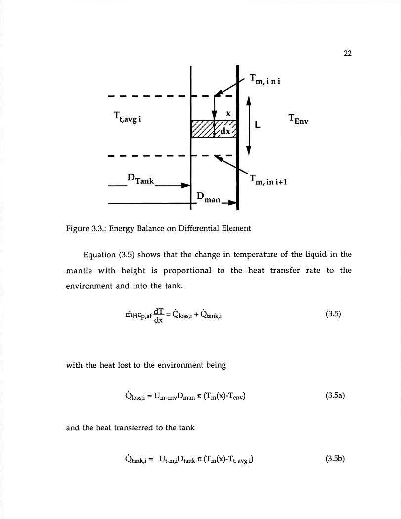
Figure 3.3.: Energy Balance on Differential Element

Equation (3.5) shows that the change in temperature of the liquid in the

mantle with height is proportional to the heat transfer rate to the

environment and into the tank.

nHCp,af = Qloss, i + takli (3.5)

with the heat lost to the environment being

loss, i = Um-envDman It (Tm(x)-Tenv) (3.5a)

and the heat transferred to the tank

Qtank,i = Ut-m,iDtank t (Tm(x)-Tt, avg i) (3.5b)

23

When the mass flow rate in the mantle is zero equation (3.5b) is adapted to

take into account the heat losses through the mantle. To account for the heat

losses from the tank through the mantle Ut-m,i is replaced with Um-envi and

Tt,avg i is replaced with Tenv. The linear differential equation (3.5) can be

solved analytically for the temperature at any vertical distance from the top of

the node. An equation for the outlet temperature (equation 3.6) can be

obtained by setting x to the node height.

Tm, out= Tw + (Tm in- Tw) e-kL (3.6)

The inlet temperature is set to the mantle inlet temperature for the first

mantle node from the top. For the following nodes the inlet temperature is

set to the outlet temperature from the node above. Tw is the weighted average

of environment and tank temperature and can be obtained from equation

(3.6a)

= Um-envDmanTenv - Ut-mi DtankTt, avgi (3.6a)Um-envDman - Ut-mi Dtank

The exponential constant k is calculated as shown in equation (3.6b).

k = I (Um-envDman - Ut-m,i Dtank) (3.6b)kficp, af

24

The equations (3.3) and (3.4) contain in the constant B (equation 3.2b) the

average mantle node temperature. This temperature is determined in a way

so that the heat transfer from the mantle to the tank and to the environment

equals the amount obtained by integrating the local temperature differences

times the heat transfer coefficient over the height of the node. The

relationship to obtain that average (or better) equivalent mantle node

temperature is shown in equation(3.7).

Tmavg Tm,in - Tw (1 - e-kL) (3.7)k L

The weighted temperature Tw and the exponential constant k are the same as

used to determine the node outlet temperature (equation 3.6) and are obtained

by equations (3.6a) and (3.6b).

3. 2. 3. Mantle Nodes with Transient Model

In contrast to model I, the temperature in a mantle node in model II is

allowed to change over the time step, but it is set to be constant over the

height of the node. The differential equation (3.8) describing this model is

very similar to the one for the tank nodes, equation (3.1).

------- Em

Tt,avg i QTankKi:

-------

DTank source

Dman-mn

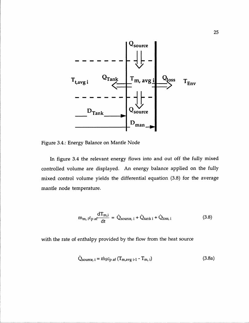
Figure 3.4.: Energy Balance on Mantle Node

In figure 3.4 the relevant energy flows into and out off the fully mixed

controlled volume are displayed. An energy balance applied on the fully

mixed control volume yields the differential equation (3.8) for the average

mantle node temperature.

dTmi _ .0mm, iCp af dt = Qsource, i + Qtank i + Qloss, i (3.8)

with the rate of enthalpy provided by the flow from the heat source

Qsource, i = ifISCp af (Tm,avg i-1 - Tm, 3)

Qsource

25

TEnv

9

(3.8a)

26

The heat transferred from the mantle to the tank can be determined as

(tank, i =-Ut-m, jAm, i (Tt, avg i - Tm, i) (3.8b)

and the heat transferred from the environment (which is usually negative as

the environment is colder than the contents of the tank) can be obtained by

Qloss, i = Um-envAenv, i (Tenv - Tm, i) (3.8c)

Equation (3.8) can be brought into the form

dTm, iCTmj+D

dt(3.9)

with C and D being constants independent of the temperature of node i

C = - (rffscp af + Ut-m, jAm, i + Um-envAenv, i)

D = - (rnscp afTm, i-1 +Ut-m, jAm, iTt, avg i

+ Um-envAenviTenv)

(3.9a)

(3.9b)

The differential equation can be solved analytically to obtain the temperature

at the end of the time step in the mantle node at every point in time.

Equation (3.10) shows how the final temperature of a time step is computed

starting with the initial temperature at the time step.

1

27

Tm, final i = (Tm, initial i + D) e(C*At) - 12 (3.10)C C

To calculate the heat transferred to the tank and the environment an

equivalent temperature is found that has a value which results in the same

heat transferred as if the momentary heat transfer rate had been integrated

over the time step. This average mantle node temperature is obtained from

equation 3.11).

(Tm, initial i + D)TM, avgi (e(C-at)lC1) -1D (3.11)magi = (c'At) C"

Like the equations for the tank nodes (equation (3.3) and (3.4)) equations (3.10)

and (3.11) are a set of coupled differential equations.

3. 2. 4. Heat Transfer Coefficient

As discussed in section 3.1.4. the heat transfer coefficient from the anti-freeze

liquid in the mantle to the water stored in the tank can be approximated with

only the heat transfer coefficient from the mantle liquid to the wall, since the

heat transfer mechanism is the major heat transfer resistance. This heat

transfer coefficient can be obtained from equation (3.12). It depends on the

conductivity of the anti-freeze liquid, on the hydraulic diameter of the mantle

which is twice the spacing between the outer and the inner mantle wall, the

local Nusselt number, and the correction factor C1. This correction factor

accounts for the fact that the empirical equation (3.14) is only an

28

approximation for the application in a mantle heat exchanger. The correction

factor C1 is fitted with experimental data.

Ut-m, i = C1 kaf Nui (3.12)Dh

Equation (3.14) provides an average value of the Nusselt number from the

starting point of the laminar flow to the point looked at. With equation (3.13)

the average Nusselt number for the ith node can be obtained. xi is the distance

from the top of the mantle to the end of the ith node.

Nui = Nu(xi)*xi - Nu(xi-1 )*xi-i (3.13)Xi - xi-1

The average Nusselt number in equation (3.14) was developed by Mercer et al.

(1976) [7]. It is intended for laminar flow between two flat plates with constant

heat flux on one side and insulated on the other.

0.0606(Re Pr Dh/x)1 "21 + 0.0909(Re Pr Dh/X)0 "7 Pr ° '17 (3.14)

Equation (3.14) depends on the flow length, the hydraulic diameter, the

Reynolds number of the flow and the Prandtl number of the anti-freeze liquid

in the mantle. The Reynolds number is a dimensionless value characterizing

the flow. As displayed in equation (3.15) it can be determined from the

hydraulic diameter, the mass flow rate in the mantle, the viscosity of the anti-

freeze liquid and the cross sectional area of the mantle.

29

Re = Dh rnih (3.15)9. Acr

The Prandtl number and the viscosity both depend on the temperature of the

liquid and they change for different liquids. They can be obtained from

temperature dependent curvefits using third order polynomials.

3. 2. 5. Temperature Inversions

The purpose of the temperature inversion algorithm is to convert an unstable

temperature distribution in the tank into a stable one, i. e. with no node being

hotter than the node above. The algorithm starts at the bottom of the tank

with its search for temperature inversions. If one is detected the mixing

temperature of the two nodes is determined. This mixing temperature then is

compared to the next node above. Should this node still be colder than the

mixed temperature it is also mixed in. This procedure is continued until a

node with a higher temperature than the temperature mix is reached. Then

all nodes from which the mixed temperature was determined are actually

assigned the mixed temperature. After that the algorithm continues its search

for temperature inversions, and treats them the same way. After the whole

tank has been investigated and the temperatures corrected if necessary the

whole tank is checked again. This final check is necessary, because the mixing

algorithm can create inversions as the mixing usually reduces the

temperature of the lowest node mixed in. Should there still be inversions the

whole process is repeated.

30

3. 2. 6. Conduction between Nodes

The conductive resistances as they are used in the term for the heat

transferred between the nodes, consist of two parallel resistances. One

resistance is for the heat transferred directly through the water from one node

to the other, and the other is a series of three resistances. The three resistances

are the resistance by the boundary between the fluid at a node and the wall of

the tank, the resistance of tank wall itself and the resistance of the boundary

between the tank wall and the liquid in the next node. The direct resistance

can be obtained from equation (3.16). To get this equation the fully mixed

model cannot be used, as for a realistic estimate of the conductive heat transfer

a constant temperature gradient over the regarded distance has to be assumed.

As distance the length between the centers of the two nodes is used.

Rdi= Axi (3.16)kH20 At

The cumulative effect of a series of resistances is obtained by summing them.

In the case of the heat transfer through the wall the resistance to the wall,

through the wall, and from the wall have to be summed. The total resistances

put up by the wall is calculated with equation (3.17).

R = 1 + Axi + 1-(3.17)hi ildtankLi kst tdtanktw hi+l 7tdtankLi+(

The total value for the resistance between the two nodes can be obtained from

the two parallel resistances with the same equation (equation (3.18)) which is

used for parallel electrical resistances.

31

1_ 1 + 1 (3.18)Ri Rd, i Rw, i

3. 3. Discussion of Chosen Assumptions

3. 3. 1. Mantle Nodes

The disadvantage of model I is, that it does not take into account the transport

time it takes for the fluid to flow through the mantle. Every change of the

mantle inlet temperature instantly effects all the nodes within the same time

step, even though it should take, for example, several time steps. The second

disadvantage is that in heating up the tank the temperature comes out a little

to high from the mantle, as the energy to heat up the tank doesn't have to be

provided. The advantage is that there is no numerical limit to the mantle

flow rate or the time step which is imposed by the mantle.

Model II takes into account the change in energy in the mantle, and it also

respects the "temperature history" of the mantle. This big advantages have to

be paid for by strict limitations to the time step or the mantle flow rate. To

obtain correct results at a given time step the flow rate can be at a maximum

so high, that it just exchanges one entire control volume in the mantle per

time step.

32

3. 3. 2. Conduction

During the normal charging and decharging cycle the influence of conduction

is hardly important for the temperature distribution in the tank. The energy

transfer through the mantle and the load flow through the tank is completely

overwhelmed compared to the conductive heat transfer. During the night

though when the flow from the source is shut off, and no water is drawn from

the tank, conduction is the only mode of heat transfer. Over the whole night

conduction has quite a significant effect. A hot temperature in a strongly

stratified tank loses in many cases more heat to colder nodes than to the

environment.

3. 3. 3. Free Convection

Heat transfer by free convection was considered as a mode of heat transfer

between the nodes. The cooling down and simultaneous destratification of a

hot water tank is simulated, assuming free convection due to the cold outside

wall would occur. The mass of water flowing from one node to the next lower

is calculated using an equation derived from a relationship for a vertical

isothermal plate in a medium of constant temperature. Every node is split up

into a center part and a boundary layer part as shown in figure 3.5.. Energy

and mass balances are applied on both.

The development of the temperature distribution is calculated using a

finite difference method. The results from the simulation are then compared

to real experimental data displayed in figure 3.6.. The simulation results are

shown in figure 3.7. The cool down and destratification characteristic in the

two graphs is fairly similar, but the time scale is almost two orders of

magnitude different. This difference shows that the free convection equation

33

Qenv =

Tenv

Qenv

\YvX.._

Ti= ml

4r~ml

m2 - mlT2

4m2

'i

Figure 3.5.: Mass flow Induced by Free Convection

for a plate at uniform temperature in a infinite medium at constant

temperature is far from being appropriate in this case. Neither analytical nor

empirical equations for free convective mass flow in enclosures could be

found, but it can be assumed that hardly any free convective mass flow occurs.

The effects of free convection are therefore neglected in the simulation model.

5U0

*1 4

35

T i imein Hor

A n ......... ..... ..... ....... .... ... ................. i... ........ .....:..

3 .25 ...

" 20

15 :W I:

0 4 8 12 16Time in Hours

Figure 3.6.". Experimental Data for Cool Down Test

50. ..

3 5 -. ............. . .......... ................. .... .

................... ..................

F-4 2 5 .........2 0 .... .. .... ... '.......... ... ..........

15 t I I-

0.2 0.3 0.4 0.5 0.6Time in Hours

Figure 3.7.: Simulation Results

34

24

35

3. 4. Algorithm

In this section the calculation procedure used in the mantle heat exchanger

subroutine is outlined. The TRNSYS-main routine calls the subroutines that

are specified in the TRNSYS-deck. The specified connections are executed by

giving the current output values of a subroutine to one or more other

subroutines as input values. During one time step the main program

compares all output values with the ones from the iteration step before. If the

maximum difference is larger than the tolerance specified the iteration process

is continued.

In its first call the mantle heat exchanger subroutine reads in the specified

parameters and initial conditions. In the beginning of every call the

subroutine reads in the required input values. At the first iteration of a time

step the temperature profile in the tank is checked for temperature inversions.

If any are detected they are eliminated according to the algorithm described in

section 3.2.5.. Also at the first iteration of a time step the initial temperature is

set to the final temperature of the time step before. In every iteration the

temperatures in the tank are calculated from the top to the bottom. In model I

(section 3.2.2.) the average temperature in the mantle is calculated first, using

the average tank temperature from the iteration before. With the new mantle

node average temperature the tank node average temperature is evaluated.

I

ParametersInputsInitial Conditions

Checking for temperature inversionsand mix all nodes above

I--

Calculating Average Temperature inMantle Node using Tavg of Tank Node

of Iteration beforeFor AllNodesFrom Calculating the New Final and Average

Top To Temperature in the Tank NodeBottom Incl. - Heat Transfer from the Mantle

- Heat Losses to the Environment- Load Flow

(Transient DEQ Subroutine Diffeq)

eiualsUsNewithin the TavgN of

NSpecified s/ TankolearancesTn

Outputs forActual Timestep

Figure 3.8.: Flow Chart of Algorithm for One Time Step

36

37

In model II (section 3.2.3) the average temperature of nodes touching the

mantle is calculated using the mantle average temperature from the iteration

before (or in the first iteration of the times step, of the time step before). To

evaluate the temperature in the tank the newly calculated average tank node

temperature is used.

I

38

4. Verification of Model

4.1. Testing of a Model

Real situations include a much broader variety of possibilities than a

computer program ever can take into account. Therefore it is impossible to

come up with reasonable assumptions without comparing the simulation

results with data from real experiments. Some additional features might have

to be included to make the model work better, others might only add to the

computation time without improving the exactness of the results

significantly.

To come up with a meaningful error value that represents the accuracy of

the simulation as the mantle heat exchanger subroutine calculates multiple

temperatures at different locations and at different points in time. Apart from

that, only temperatures at some particular spots are recorded in real

experiments. The values for the change of energy stored in the tank, the

energy extracted from the tank, and the losses to the environment can be

calculated from the temperatures in the tank node at different time steps. The

energy going into the mantle can be determined from the difference of the

39

inlet and outlet temperatures of the mantle. Therefore the state of the tank

can be completely described with the values of the temperatures in the tank

nodes, and the outlet temperature of the mantle assuming the inlet

temperatures from the solar collector and from the mains are known.

Therefore it is sufficient to take into consideration only the values of these

temperatures for error calculations. For short tests (over a time period of less

than one or two days) there are two possibilities to determine a useful error

value for the simulation exactness. One is to calculate the average of the

squared residuals of the temperatures for the nodes at certain times. This

method is very similar to the least squares method. The alternative to that is

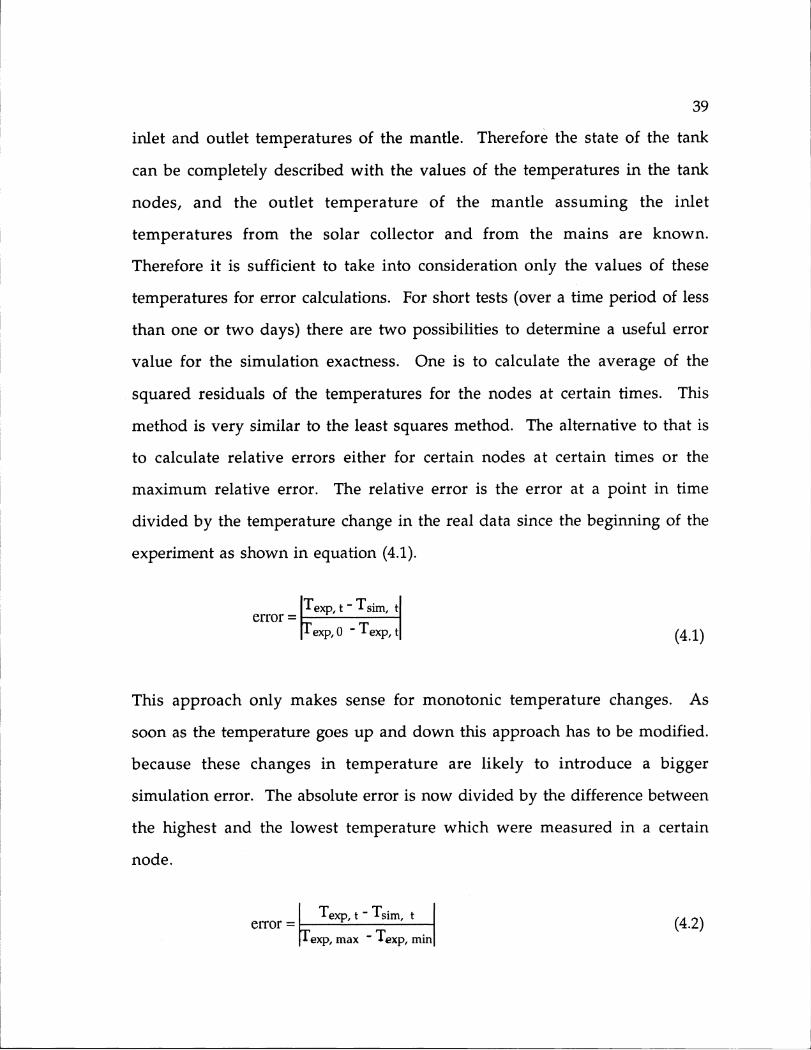
to calculate relative errors either for certain nodes at certain times or the

maximum relative error. The relative error is the error at a point in time

divided by the temperature change in the real data since the beginning of the

experiment as shown in equation (4.1).

Texp,t smterror = iexp, 0 - Texp, t (4.1)

This approach only makes sense for monotonic temperature changes. As

soon as the temperature goes up and down this approach has to be modified.

because these changes in temperature are likely to introduce a bigger

simulation error. The absolute error is now divided by the difference between

the highest and the lowest temperature which were measured in a certain

node.

erro=[_Texp, t - Tsim, t(42

Fexp, max - Texp, min

40

When judging an error which was obtained with equation (4.1) or (4.2) it has

to be kept in mind that the error accumulates during the simulation. For that

reason the error is expected to be larger toward the end of the simulation.

4. 2. Experiments with Low Collector Flow Rates

Experiments with mantle heat exchangers have been performed by S. Furbo

and P. Berg in the Thermal Insulation Laboratory in Denmark [1]. In their

tests they use low flow rates through the solar collector of, for example,

25 liters per hour in the experiment described in section 4.2.1.

The experiments used in this chapter are idealized in a sense that the

influence of the permanently changing solar intensity is eliminated by

supplying the mantle with water of a constant temperature. The three

experiments represent results from different operation situations. In the first

experiment a tank at a uniform low temperature is heated. The second

experiment imitates a day cycle with a hot mantle inlet temperature during a

part of the experiment, and two hot water draws out off the tank. In the third

experiment, the decay of stratification during a 24 hour period is investigated.

The tank is not exposed to draws nor a flow through the mantle. All three

experiments have been performed with a 200 liter (53 gallon) tank as displayed

in Figure 4.1. The cylindrical tank is 1.2 m (3.45 ft) high and 0.46 m (18.1 in) in

diameter. An annulus shaped mantle as described in section 2.2. is welded

around it. The mantle covers the tank over a height of 0.91 m (35.8 in)

positioned 0.1 m (3.94 in) from the bottom and 0.19 m (7.48 in) from the top.

I

41

The outer diameter of the mantle is 0.50 m (19.8 in). The thickness of the tank

wall is 5 mm (0.20 in); the thickness of the mantle wall is 3 mm (0.12 in). The

inlet to the mantle, where the hot anti-freeze liquid from the collector enters,

is right at the top of the mantle. The outlet from the mantle is at the bottom

of the mantle on the opposite side of the tank to reduce short circuiting of the

hot water in the mantle. The inlet to the storage tank, where the cold water

from the mains enters is in the middle of the bottom surface of the tank. The

outlet from the tank, where the hot water for the load is extracted, is in the

middle of the top surface. The tank is isolated. The heat loss coefficient of the

insulation material at the sides of the tank is 0.89 W/m 2K. At the top it is

1.79 W/m 2K and at the bottom 2.79 W/m 2K. The material of the wall is

Figure 4.1.: Hot Water Storage Tank with Thermocouples

42

assumed to be plain carbon steel with a conductivity of 60 W/mK. The heat

transfer coefficient from the heat exchanger surface to the liquid in the tank is

set to be 2000 W/m 2 K, which is equivalent to setting the resistance at that

place to zero.

The mantle tank in the Thermal Insulation Laboratory has been equipped

with thermocouples (the positions of the thermocouples are represented by

crosses in Figure 4.1.). Water is used for both mantle flow and hot water

storage in the tank in this experiment.

The temperatures obtained experimentally are measured at a position

close to the middle of the tank. The model predicts the average temperature

in a node, which is not necessarily equal to the temperature at the middle of

the node. With the current model it is not possible to account for temperature

changes in radial direction. To limit the influence of the temperature change

in vertical direction, relatively small control volumes are laid symmetrically

around the thermocouples reaching 2.5 cm (1 in) up and down from the

location of the thermocouples. This control volume thickness of 5 cm (2 in)

was chosen to obtain a node temperature which is close to a temperature that

would be measured in the center of the node. On the other side there is a

limit to how small the control volumes can be chosen, as numerical problems

occur for too small control volumes. The control volumes between the ones

with thermocouples are not split up and their size is therefore fixed.

43

4. 2. 1. Heating Experiment

4. 2. 1. 1. Description of Experiment

In the heating experiment, the temperatures in the tank are initially between

27 'C and 30 'C. Apart from a transient effect during the first hour, the mantle

inlet temperature is fixed at 49.3 'C. The flow rate in the tank is at roughly

30 liters/hour. During this test there are no draws from the tank. The

temperatures measured by the thermocouples in the tank are displayed in

Figure 4.2. The top temperature curve represents the output from the

thermocouple at the top of the tank, the second curve represents the output

from the second thermocouple and so on. This thermal stratification follows

nicely what would be expected from the physical laws described in section

2.1.2.

The hot liquid flowing through the mantle heats the tank from the top to

the bottom because the liquid in the mantle cools as it heats the upper nodes.

When the temperatures of the upper nodes get closer to the temperature in

the mantle the lower nodes are heated. The temperature at the outlet of the

mantle which is displayed in Figure 4.3, never cools to the temperature of the

second thermocouple from the bottom which is at the height where the

mantle ends. The outlet temperature of the tank is always between the

temperature of the second and third thermocouple from the bottom. At the

end of the experiment the temperature in the tank and the mantle almost

reach a steady state, in which all the energy that is transferred from the mantle

to the tank is lost to the environment.

....... ...... ............................ ....... ...

........ ......... .... ...... ...... ................... ..... .............................. ... ................................ ..................................

0 5 10 15

Time in Hours

Figure 4.2.: Temperature of the Tank Nodes

50

U0 4 0 o ................................ i........................ /..... ...................

.......... .................. ..................................

0 3 5 --------------30 -

S 3 0 ............. ................... ". ............................... ............................ ....

25 r0 5 10 15

20 25

20 25

Time in Hours

Figure 4.3.: In- and Outlet Temperature of the Mantle

44

50

45

• 40

435

30

25

45

The set up of experiment 1, as described in this and the preceding section,

is specified in the according TRNSYS-deck in Appendix B. The only

modifications were to halve the number of derivatives for model I, and to

change the heat transfer correction factor C1.

4. 2. 1. 2. Simulation Results for Model I

The temperatures in the tank nodes during the experiment are plotted in

Figure 4.4 together with the simulation results for the same experiment. The

simulation used a heat transfer correction factor of C1 = 1.0. For this value of

C1, the shape of the simulated curves and their matching with experimentally

obtained curves is optimized. The optimization was done by plotting the

simulation results for different correction factors together with the

experimental data and picking the set of curves with the smallest deviation

from the experimental data. With the exception of the temperature at the

tank bottom, the simulated temperatures are always higher than the

respective experimental results. The error defined in equation (4.1) is large

in the beginning for the nodes in the middle of the tank. The maximum error

then decreases to roughly 6 % at the end of the simulation. Temperatures in

the mantle nodes and the inlet temperature to the tank are shown in

Figure 4.5. No temperature measurements were taken in the mantle,

therefore only the simulated values of the temperatures in the mantle are

shown. The simulated temperature at the mantle outlet is compared to the

measured temperature. The simulated temperature is substantially higher

throughout the run. It is surprising that the simulated temperature is higher

because an energy balance would show, that for similar losses, and a faster rise

50

45

40

35

u

0

0v.

0 VW

30 -

250 5 10 15 20

Time in Hours

Figure 4.4.: Tank Node Temperatures with Model 1 and C1=1.0

u

"-4

H

50

45

40

35

30

255 10 15 20

Time in Hours

Figure 4.5.: Mantle Node Temperatures with Model 1 and C1=1.0

46

25

.........; . ................ .... .......... .............. ....... ......... .... ....... ............... ........... t2.. . . . .f - - . - . .-- F _:-:" .. :':- -.:'----" -- " --

......:'........ ..... ': ...... .. .......... :.:. .... ... . .'........... .. ...... 4 ........... .." .- ,................. ..... .. t

......:.. .... ........ .... ....................... .. .... .................................. .. ..................................

!/ ." ," ,:" - '-tout

A.-.-------- ................ .......... +.................................... ........................ ......... ..................................iExperimental Data. Full Lines

-• Simulation Results: Dashed Lines

25

47

30

50 d

i .: - :. . .. ." _ - -........ ' - : : - " ,".. ..............., ....... .

45-..... ... -.. .. . ..4 5 .......... ........... " .... . ..... ... ' " .......... ......... ... "" .................... .... ..................................

- 0 ........ '-'... .. "' " .... ......... :" ... ... ... .................. ..... :..-i........ ........................ ...... ............................

... ... ....... ". .. ..................... .. ................................ i. ............................ L..................................

30 . .... .... .

35O

Experimental Data: Full LinesSimulation Results: Dashed Lines

2 5 . . . . . . . .. . . . .

0 5 10 15 20 25

Time in Hours

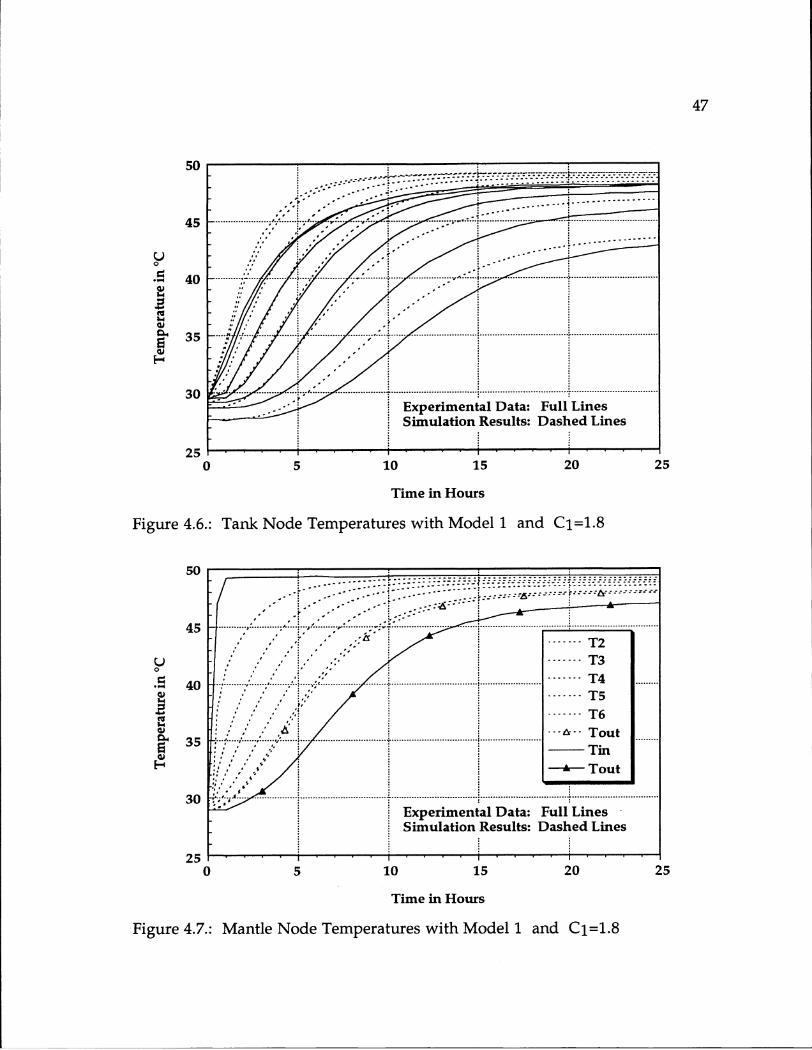
Figure 4.6.: Tank Node Temperatures with Model 1 and C1=1.8

450 ....... ...... ............. ... .. .... ... ............................... ................. .

4 5 ..... -.... ...... .. .... "---,: ........ -........................ ........ ; ................................. ........................ T 4.........

............,....f ..... .. T ou

... ................. ..................... .......... -i..... --............. ....... ..................... ............ ...................................Experimntal D ta-,.Ful.LineSimulation Results: Dashed.Line

25 ' °

48

in internal energy in the simulation (which is equivalent to a rise in

temperature of the tank nodes) the calculated energy input in the mantle

would be higher than in the experiment. However the mantle outlet

temperature in the simulation which would be expected to be lower is actually

higher than in the experiment. If the mantle outlet temperature is higher, the

temperature difference between in- and outlet decreases and with it the energy

put into the tank. The energy that seems to disappear in the experiment is

needed to heat the mantle. The problem lays in the assumption that the flow

through the mantle is at steady state during every time step. Therefore the

temperature of the liquid in a particular control volume in the mantle is

constant during a time step. Consequently the internal energy in the mantle

cannot change within the time step either. This effect is only a problem in

simulations for short time periods. As soon as the system goes through more

than a couple of energy cycles, meaning that after being heated up the tank is

cooled again, the effect becomes less important. The storage in the mantle in

this case can be regarded as an increase in the total storage capacity.

Another problem with model I can be seen in Figure 4.5. In this steady

state model the temperatures in all mantle nodes react immediately when the

mantle flow starts even though in the experiment it takes approximately an

hour for the water to travel from the top of the mantle to the bottom at the

experimental flow rates.

To obtain Figure 4.6 and 4.7 the heat transfer coefficient between mantle

and tank was increased by changing the correction coefficient Cl from 1.0 to

1.8. The results of this simulation are shown here even though they are a lot

worse than with the correction factor 1.0, because Ci = 1.8 is used in model II.

The temperatures in the upper nodes of the tank rise much faster in the

49

beginning when the higher heat transfer coefficient is applied. The rise in

temperature in the lower nodes and at the mantle outlet is delayed because

the mantle fluid transfers more energy at the top of the mantle. Slightly

higher final temperatures are reached.

4. 2. 1.3. Simulation Results for Model II

The temperatures in tank and mantle obtained with model II are shown in

Figure 4.8 and 4.9 together with the experimental results. Compared to

model one the simulated curves follow the experimental results closely. The

absolute value of the deviation between experiment and simulation never

exceeds one degree. At the end of the simulation the maximum relative error

from equation (4.1) is roughly 3 %. The predicted temperatures in most tank

nodes and at the outlet of the mantle are slightly higher than the

temperatures obtained in the experiment, but the simulated and experimental

results are much closer together than in model I. Nevertheless these results

indicate that the heat loss coefficient to the environment in the experiment

was slightly higher than the one assumed for the simulations.

In Figure 4.8. the simulated temperature of mantle node 6 (T6) and the

simulated mantle temperature (Tout) are identical, because model II assumes

the mantle nodes to be fully mixed.

5 10 15 20 25

Time in Hours

Figure 4.8.: Tank Node Temperatures with Model 2 and C1=1.8

10 15 20 25

Time in Hours

Figure 4.9.: Mantle Node Temperatures with Model 2 and C1=1.8

50

50

45

40

S35

30

250

5o

45

U

005- 40

I435

30

250

.............. ...... ..... .A.... ...... ....... ................" .." ..." .'" . ...... t3

... -........... :. ... ....... :.". V .. . ... ........ ... ........ ....................... i...... .................. "...... t4 ...........

7~ ~ e ........ . .............. ................. t u ...........

..... ............. ......... ..... .. .. ........................................ .................................. ............................ .. .. uExpeimetalDat: Fll inSiuato Reut: ahd ie

51

4. 2. 1. 4. Comparing Simulation Results from Model I and Model II

To make it possible to compare model I and model II, model I was also

simulated for C1=1.8 as shown in Figure 4.6 and 4.7. Model I treats the flow

through the mantle as being in steady state throughout the time step whereas

model II accounts for the energy stored in the mantle nodes. This storage of

energy in the mantle is the reason why the simulation using model II yields a

much slower temperature rise in the tank as well as in the mantle nodes.

Towards the end of the simulation however one would expect that the two

models should converge because a steady state is almost reached. But the tank

node temperatures and the temperature at the mantle outlet are calculated to

be between half and one degree higher after 25 hours for model I compared to

model II. The reason for that difference is that even in a steady state the

average temperature in a mantle node are calculated differently. In model I,

the temperature is calculated for every position and then the average

temperature over the height of a node is determined. In model II the mantle

nodes are considered to be fully mixed, and the time average is used to

determine the heat transfer to the environment and into the tank. For that

reason model I should provide improved results in cases like here at the end

of this experiment where the steady state is approached.

The computational effort for the two models is very similar, provided the

same time step is used. For a time step of 1/64 of an hour the tank subroutine

is called 3330 times for the 26 hour simulation. 3330 calls mean exactly two

calls per time step, which is the minimum for modules that have to be

checked for convergence. The run, that uses model I takes 26.3 CPU seconds

and a run with model II takes 28.2 CPU seconds.

52

4. 2. 2. Experiment with Draws

4. 2. 2. 1. Description of Experimental Set Up

This experiment approximates normal operation of a energy store in a solar

domestic hot water system. The temperatures in the tank are initially between

16.5 °C at the bottom and 19.1 'C at the top. The mantle flow rate is, with

small variations, 23.5 liters/hours. The temperature at the mantle inlet is

30 'C for the first hour and 45 minutes. It is then set to 70 'C for four hours,

and finally set back to 30 C for the rest of the experiment as it can be seen in

Figure 4.11. The load flow is imitated by two 50 liter draws, the first after one

hour and the second after 3.5 hours. The water which is drawn, is replaced

with water from the mains at 14.2 'C. These draws cause the steep temperature

drops in the tank in Figure 4.10. After 6.5 hours the mantle inlet temperature

is smaller than the temperature in tank so that it actually cools the tank. It is

surprising that the two bottom nodes in the tank, and the mantle outlet

temperature are hardly effected either by the draws or by the big changes in

mantle inlet temperature.

4. 2. 2. 2. Simulation Results from Model I

In Figure 4.12, the simulated temperatures obtained with model I and a heat

transfer correction factor of one are plotted together with the experimental

results. The simulated temperatures during most parts of the experiment are

between two and three degrees higher than the corresponding measured

temperatures. Most of the simulated temperature curves are closer to the

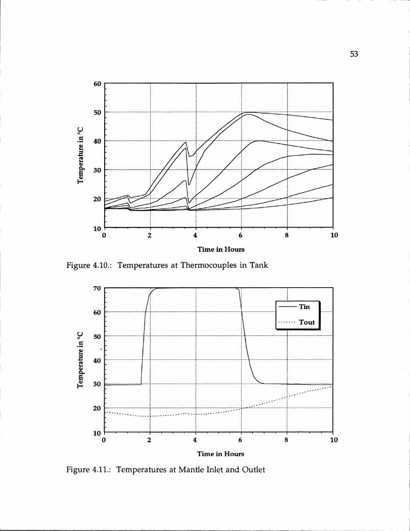
60

50

00- 40

! 30

20

10

. ............... ,..............................

. . . . . . . . . . . . . . . . . . . . . . . ...... ... ...... ... ...... .... .e ... .. .. ... ... ... ...... ... .. ..... ... ... ... ... ... ... ... ...... ...

.......... ............. . ....... .. ........... ........ ....... ............ -------- ......

...........

0 2 6 810

Time in Hours

Figure 4.10.: Temperatures at Thermocouples in Tank

70

60

50

. 40

E 30

20

10 . . . . , . , ,0 2 4 6

Time in Hours

Figure 4.11.: Temperatures at Mantle Inlet and Outlet

10

53

54

temperature curve measured in the node above. In contrary to the

experimental data, the simulated temperatures of the two bottom nodes and

of the mantle node react strongly (with temperature drops) to the two draws.

They also react stronger to the change in mantle inlet temperature than

observed in the experiment. The simulated mantle node temperatures and

mantle outlet temperature are plotted in Figure 4.13. The mantle outlet

temperature is apart, form some periods during the first two hours always

higher than the measured mantle outlet temperature. As in the heating

experiment this effect is caused by the inability of model I to account for

energy storage in the mantle. After 6.5 hours the mantle inlet temperature

drops to 30 'C, and the temperature in the top two mantle nodes (T2 and T3)

fall below the temperatures in the lower mantle nodes. This situation can

occur as there is no algorithm that prevents temperature inversions in the

mantle. It is assumed that under most flow conditions the flow velocity and

liquid viscosity are high enough to sustain the inversions. In reality, some

mixing occurs, but unfortunately the temperatures in the different mantle

nodes were not recorded during the experiment.

In Figure 4.14. and 4.15 the results for the simulation with a correction

factor C1 = 1.8 are shown. As expected for a higher heat transfer coefficient the

temperatures in the higher tank nodes are higher than for C1 = 1.0. The lower

tank nodes are heated slower because, due to the high heat transfer coefficient,

more energy is transferred to the higher nodes and consequently the

temperature in the mantle is lower once it reaches the lower nodes. For this

reason the simulated temperatures in the mantle nodes are lower than for Ci

= 1.0 during periods with a high mantle inlet temperature and they are higher

for the low mantle inlet temperature after 6.5 hours.

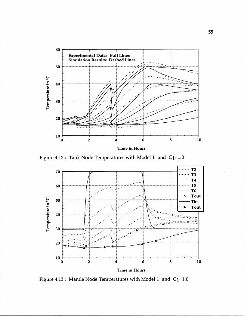
55

60 ___

- Experimental Data: Full Lines- Simulation Results.- Dashed Lines

5 0 ................................ .... ............ ..........T .. .... ......... .. .... ...... ....................40 ... ............

. . . . . .. . . . . .. . . . .. . . . ..... . ... .. . ............ ........ .I--" .. . . . .. . . . .. . .-3 0 .-...............................

.. . . . .. . . ... . . . .. . . . .. J,. ... ..... .... ... . . ....... . ......... . ..... .. ................. .... .

10

0 2 4 6 8 10

Time in Hours

Figure 4.12.: Tank Node Temperatures with Model 1 and C1=1.0

70 ------- T2----T3

T46 ................ ...................... ............ ...... ....:-. .."": : .......................................... T ,560 -............. T5... .

-"T6----- Tout0 ............................ ... V .................................. .-................ .................s ..................................*1 ........

0 so Tin-"" - Tout

4 0 ......................... :.... i........ .... ............... -i-........... ;--. .................. .. ..... ... .. ".... ."..... : ..- ,..- ............................40 - ....- ....... .-.

'lop --------....." . -'........ ...... " i ... _ " . ....................._ 3 0 - ............-.....-

....... e ...

1001 ........... ......................... . ............ . . . . .....

0 2 4 6 8 10

Time mn Hours

Figure 4.13.: Mantle Node Temperatures with Model 1 and C1i=1.O

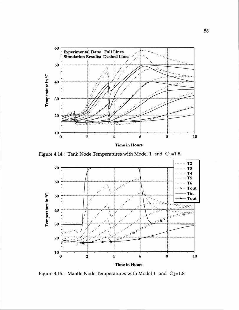
60

50

u

- 40

S30

20

102

Time in Hours

Figure 4.14.: Tank Node Temperatures with Model 1 and C1=1.8

70

60

50

40

E 30

20

10

10

2 4 6 8 10

Time in Hours

Figure 4.15.: Mantle Node Temperatures with Model 1 and Ci=1.8

56

-Experimental Data: Full Lines . .

Simulation Results: Dashed Lines -

. . .. . . . . .. .. ... .. .. . ...... .. .. ... .. .. . . .. .. .. ....

................................ ............. ............... .... ... ........ ........ .. .. .. ............. ... .................... . '--- L

. ................... .. . ".. .....P " .... ".......... ....... .. ................. ..... ....

. ... ... ...... ..... ....i} .. ......... ; .. .. . ... ....... &r.. ..."....." .... ".---...... .. .. ..........

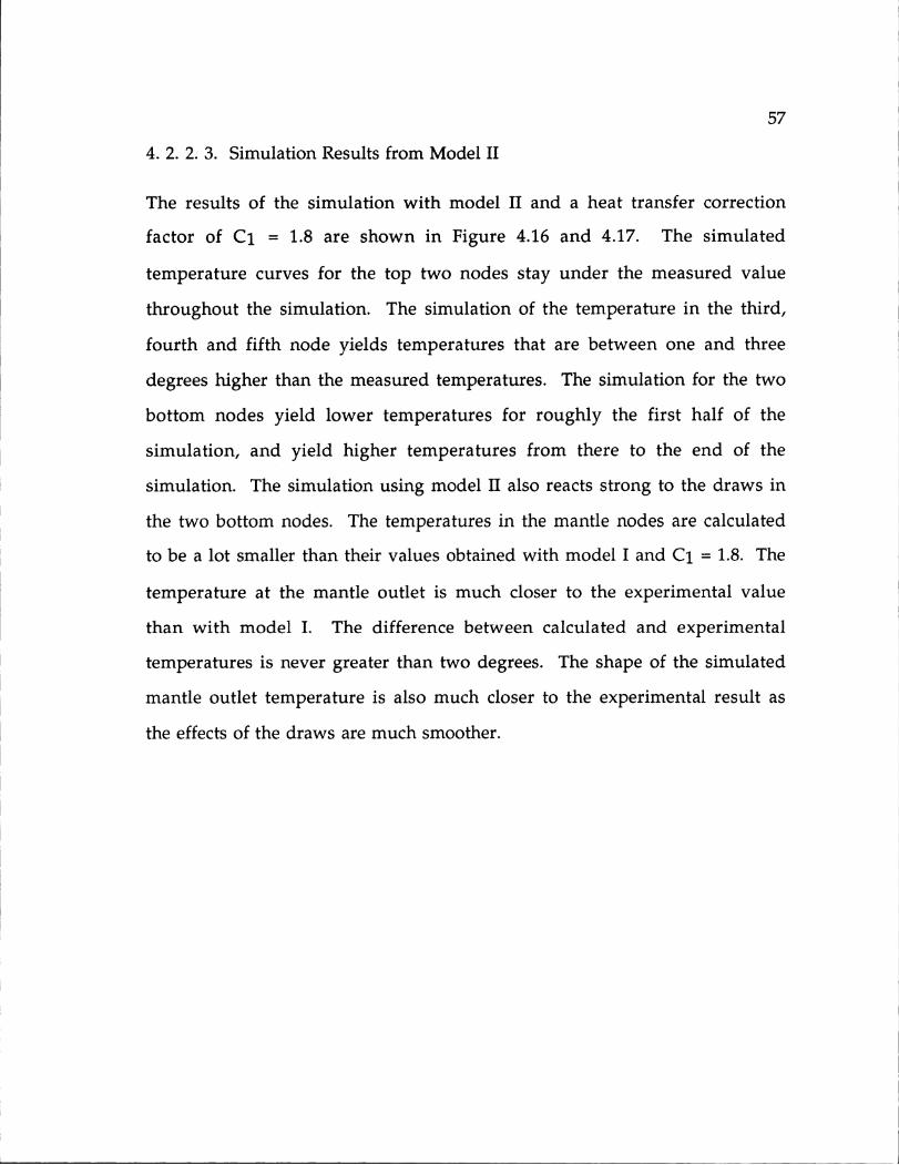
57

4. 2. 2. 3. Simulation Results from Model II

The results of the simulation with model II and a heat transfer correction

factor of C1 = 1.8 are shown in Figure 4.16 and 4.17. The simulated

temperature curves for the top two nodes stay under the measured value

throughout the simulation. The simulation of the temperature in the third,

fourth and fifth node yields temperatures that are between one and three

degrees higher than the measured temperatures. The simulation for the two

bottom nodes yield lower temperatures for roughly the first half of the

simulation, and yield higher temperatures from there to the end of the

simulation. The simulation using model II also reacts strong to the draws in

the two bottom nodes. The temperatures in the mantle nodes are calculated

to be a lot smaller than their values obtained with model I and C1 = 1.8. The

temperature at the mantle outlet is much closer to the experimental value

than with model I. The difference between calculated and experimental

temperatures is never greater than two degrees. The shape of the simulated

mantle outlet temperature is also much closer to the experimental result as

the effects of the draws are much smoother.

60

50

s•*- 40u

'40

~30

20

102 4 8 10

Time in Hours

Figure 4.16.: Tank Node Temperatures with Model 2 and C1=1.8

70 , :

60

50so

40

20

102 4 6 8 10

Time in Hours

Figure 4.17.: Mantle Node Temperatures with Model 2 and C1=1.8

58

Experimental Data: Full LinesSimulation Results: Dashed Lines

. ..............................--.- ----..... .......... .... ..... ..... .... ..............

-4.............. .... .............................. ..... .. . . .......... 40 ... ............... ..

....... .... 044 .. ........ .... , .. ......... .. -... " ......

iiii/

-77 -7 .". -:.' ' :. -' ' .-. " -.- " . . . . . .--- ----

......... ........... ..... ...............

_ I _ _ . I . . .. . . t • • •

59

4. 2. 3. Cooling Experiment

4. 2. 3. 1. Description of Experiment

In this test, not only the cooling of a tank filled with hot water is investigated,

but also the decay of thermal stratification over time. The stratification of the

tank that is originally at an almost uniform temperature of 48 'C, is obtained

by tapping half of the volume of the water and replacing it with cold water

from the mains at 16.8 'C. The initial situation obtained by this procedure is

that the top half of the tank is at temperatures between 44 'C and 48°C and the

bottom half is at temperatures between 19 'C and 22 °C. After the draw in the

beginning no more water is drawn nor is any water run through the mantle.

The top nodes of the tank cool down due to losses to the environment but

they also loose energy to the lower nodes by conduction. The heat conduction

from the top nodes heats the lower nodes.

4. 2. 3. 2. Simulation Results from Model I and Model II

The simulation results for model I with C1 = 1.0 and for model II with C1=1.8

are plotted in Figure 4.18 and 4.19, respectively. Results from simulations

with model I and C1=1.8 have not been plotted as they are not visibly different

from simulations with C1 = 1.0. The simulation results from the two models

are fairly similar to each other and therefore discussed in one section. The

similarity is not surprising as the difference between the two models is the

way the mantle is treated when the flow rate in the mantle is non-zero. Both

models equally underpredict the speed of the stratification decay. That means

50

45

40

0

0 3530

S25

20

15

104 12 16 20

Time in Hours

Figure 4.18.: Tank Node Temperatures with model 1 and Ci=1.0

50

45

40

35

25

20

15

104 12 16 20

Time in Hours

Figure 4.19.: Tank Node Temperatures with model 2 and C1=1.8

60

i . . . .. ................. ..............

........................... .......................................................................l ....... ..............-~~~ -- SimlationResult:-Dashd-Line

--..:..• . .. ..

. . .. " i........'.".'....."....... "."...".

24

. ...... . . . .... ........ .

..". ... .. . ......... ........ .,...

.. ............. ........ ........ ........ .... .... .. ...... ........ ............-----

" ................. "..................... ...-.................

-~~~ ....................................................................pe im entalD ata:.Fll.Lin e

. ............. Experimental Data: Full Lines .......Simulation Results: Dashed Lines

24

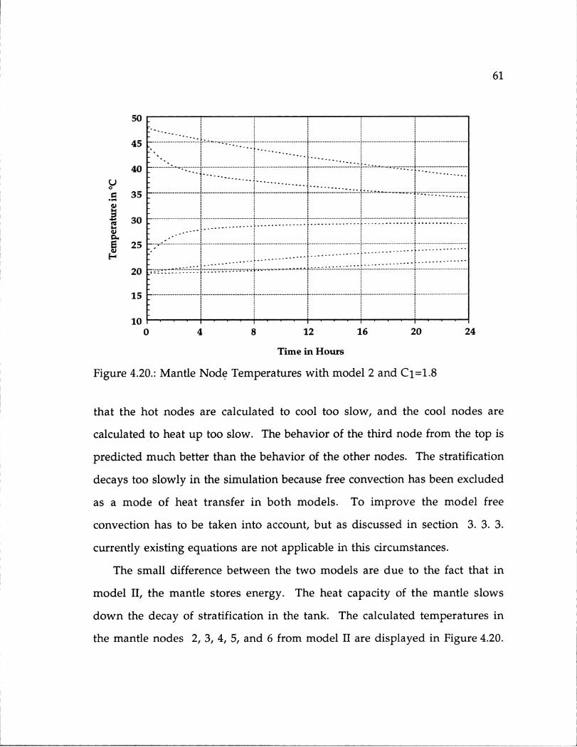
61

50

45

40o

35

( 30

25

20

15

InI V I I" " I"I I I lII

0 4 8 12 16 20 24

Time in Hours

Figure 4.20.: Mantle Node Temperatures with model 2 and C1=1.8

that the hot nodes are calculated to cool too slow, and the cool nodes are

calculated to heat up too slow. The behavior of the third node from the top is

predicted much better than the behavior of the other nodes. The stratification

decays too slowly in the simulation because free convection has been excluded

as a mode of heat transfer in both models. To improve the model free

convection has to be taken into account, but as discussed in section 3. 3. 3.

currently existing equations are not applicable in this circumstances.

The small difference between the two models are due to the fact that in

model II, the mantle stores energy. The heat capacity of the mantle slows

down the decay of stratification in the tank. The calculated temperatures in

the mantle nodes 2, 3, 4, 5, and 6 from model II are displayed in Figure 4.20.

.. --:: .,........ ............... ........... .. .. .. .. .. .. .. .. .............................. ............................. ... .. .. .. .. .. .. .. .. .. .. .. .. .

........................... ............................ ............................ ............................ .................... . ~ :::: ......

........................... .. ....................................... ........................ .............. ... .. ....... .............. .

_. ................ ............................. ............................ ............................. .................. .. ... .............................o . .. .. .. .. .. . --. --.-.. -.-..-.- ...

[ ........................... . ... .... ........... ........... .............. .

............. ............... ............................. ............................ ............................. ............................. ............................

6I

62

As the temperature changes are very slow the mantle temperatures are almost

identical with the simulated temperatures in the tank.

4. 3. Experiment with Regular Flow Rates

4. 3. 1. Description of Experiment

A series of indoor experiments with solar systems have been performed in the

Solar Calorimeter Laboratory. A solar simulation facility has been used for

these experiment to have control over the environmental conditions. The

experiment, which was simulated for this thesis was run during a period of

24 hours. The conditions during the experiment imitate the operation

conditions of a typical day. The amount of incoming solar radiation in the

experiment is equivalent to an average day in March in Madison, Wisconsin.

Water is drawn to meet a standardized load at every hour between 7 am and

1 pm and between 4 pm and 9 pm. The draws are between 5 liters and 45 liters

and total 225 liters for the whole day. The distribution of the draws is

displayed in Figure 4.22. To exclude simulation errors from the solar collector,

only the tank has been modeled in this simulation.

The storage system used is a tank-in-tank system similar to the one

described in section 2.2. The tank-in-tank system is shown in Figure 4.21. The

inner tank has a volume of 208 liters and the shell contains 19 liters. The

height of the inner tank is 1.48 m, and the total height is 1.54 m. The diameter

of the inner tank is 0.44 m. The boundary wall between shell and inner tank

is 1.6 mm thick and undulated to increase the heat transfer coefficient and the

heat exchanger surface. Due to the undulation, the smallest distance between

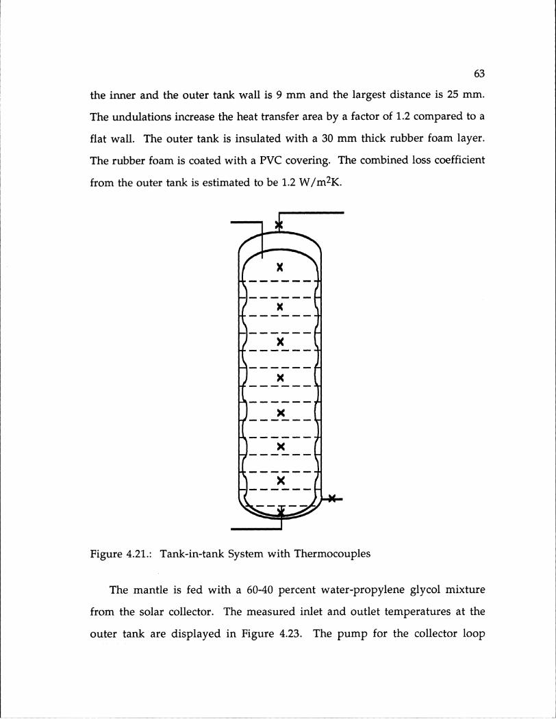
63

the inner and the outer tank wall is 9 mm and the largest distance is 25 mm.

The undulations increase the heat transfer area by a factor of 1.2 compared to a

flat wall. The outer tank is insulated with a 30 mm thick rubber foam layer.

The rubber foam is coated with a PVC covering. The combined loss coefficient

from the outer tank is estimated to be 1.2 W/m 2K.

Figure 4.21.: Tank-in-tank System with Thermocouples

The mantle is fed with a 60-40 percent water-propylene glycol mixture

from the solar collector. The measured inlet and outlet temperatures at the

outer tank are displayed in Figure 4.23. The pump for the collector loop

64

operates between 8 am and 4 pm as shown in Figure 4.22. The storage tank is

fed at the bottom with replacement water from the mains at a temperature of

18 °C. The eight thermocouples in the tank are positioned at the bottom of the

tank and than at distances of 0.2 m above each other. The tank-in-tank system

is approximated by using the mantle heat exchanger model for a mantle

which extends from the shell outlet to the top of the tank . This procedure

introduces an error in the determination of the temperature in the top node,

as only the side walls of the heat transfer surface at the top node are used for

the simulated heat transfer. For the numerical simulation the volume in the

tank was split up into fifteen control volumes. All of the nodes except the top

and the bottom node, have a thickness of 0.1 m and the thermocouples are

positioned in the center of the node. The temperatures measured by the

thermocouples in the tank during the experiment are displayed in Figure 4.24.

100 - -

mheat- ...... ...... . .............. 2 0 -f80 4.. 1 162024 .............

. 6 0 .......................... ............................. 'i ........... .. .......... ............................. ............ .............. ............................:w

Time in Hours

Figure 4.22.: Mass Flow Rate of Load and of Heat Source

65

60 ____

50....Tman-out50 ........................... ............................. ......................... I. ...... . ................... ...... T m an -in .

-, 4 0 .............. ........ ............ .... ........... ". " ... t..... .... .............. .................

2 0 ..... ........................... .......................................... ............ .. ..I............................40 -

30......',

0 4 8 12 16 20 24

Time im Hours

Figure 4.23.: Mantle Inlet and Outlet Temperature

0

3 0 ........................... :. ......................... ..... .. ..... ......... .... .... ......... ............ .. ..... ...... ..... .... ..... .......................

2 ..................... ....... ... .. ...................... ............ ....... "- ................ ..

'-4

10 . • . ..

0 4 8 12 16 20 24

Time mn Hours

Figure 4.24:" TMpatres etasuretb ThermoculesnTn

66

4. 3. 2. Simulation Results with Model I

In Figure 4.25a and 4.25b, the temperatures in the inner tank nodes obtained

with model I and a heat transfer correction factor C1=1.0 are plotted together

with the experimental results. The temperature curves for nodes 1, 3, 5, and 7

are shown in Figure 4.25a and the curves for nodes 2,4,6, and 8 are shown in

Figure 4.25b in order to make it easier to read the graphs. The first seven

hours of the experiment are very similar to the cooling experiment discussed

in chapter 4.2.3 as there is no draws and no flow through the shell. During the

period with flow through the shell (from 8 am to 4 pm) the temperatures in

the inner tank are underpredicted by one to four degrees. The calculated

temperatures of the top and the bottom node differ from the measurements by

as much as 160 C. The top node is underpredicted by a maximum of seven

degrees and the bottom node is underpredicted by 16 degrees at the worst

point. This strong deviation results from the fact that the mantle heat

exchanger model does not account for the heat transferred through the top of

the inner tank. As the mantle is specified to have its lowest point at the shell

outlet, the bottom node is not surrounded by the shell. This specification was

chosen to get a good estimate of the shell outlet temperature sacrificing

exactness in the simulation of the bottom node, as the bottom node, in reality,

is surrounded by the mantle.

For the period with no flow through the shell but with draws the

calculated temperature of most nodes is relatively close to the experimental

data. The exceptions are the simulation results for the inner tank nodes 2, 3

and 5. The simulated temperature values are too low for node 2 and 3 and too

high for node 5. The experimental tank has a higher degree of stratification

L

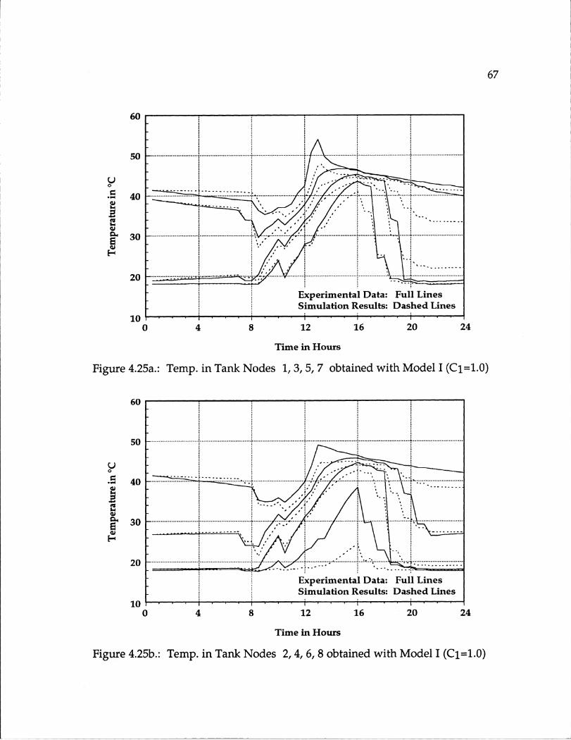
67

50

o40

, 30 ..............

20iExperimental Data: Full Lines

_ iSimulation Results: Dashed Lines

100 4 8 12 16 20 24

Time in Hours

Figure 4.25a.: Temp. in Tank Nodes 1, 3, 5, 7 obtained with Model I (CI=1.0)

60

20.... . . .... , i • ...

10 1

0.4..8..12..16..20...24

Time in Hours

Figure 4.25b.: Temp. in Tank Nodes 2,4,6,8 obtained with Model I (C1=1.0)

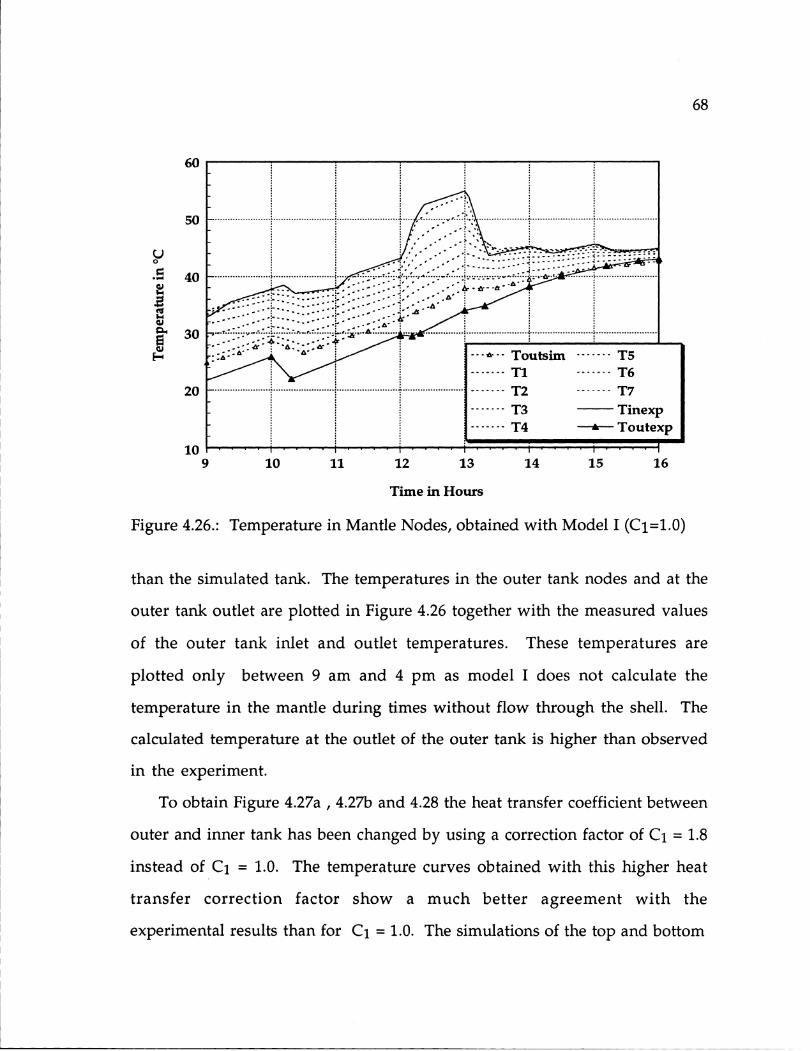
68

60 .. ... .. .. .... .... ............... ................... C... ..... .. r .. ................. ......................... i... .....................T4 . -- To..t

.............. ..... ...................... ...... -.......... ..... ... ......".... ....1400.1..12.13.14 15 16

. .: ." ... ... . ...... .- :, °.. -...".............................................. ----------

30 ........ ........

. ::.,- • A- i"" '"Toutshn . ......--T5

T1 T

9 10 11 12 13 14 15 16

Time in Hours

Figure 4.26.: Temperature in Mantle Nodes, obtained with Model I (C1=1.0)

than the simulated tank. The temperatures in the outer tank nodes and at the

outer tank outlet are plotted in Figure 4.26 together with the measured values

of the outer tank inlet and outlet temperatures. These temperatures are

plotted only between 9 am and 4 pm as model I does not calculate the

temperature in the mantle during times without flow through the shell. The

calculated temperature at the outlet of the outer tank is higher than observed

in the experiment.

To obtain Figure 4.27a , 4.27b and 4.28 the heat transfer coefficient between

outer and inner tank has been changed by using a correction factor of C1 = 1.8

instead of C = 1.0. The temperature curves obtained with this higher heat

transfer correction factor show a much better agreement with the

experimental results than for Ci = 1.0. The simulations of the top and bottom

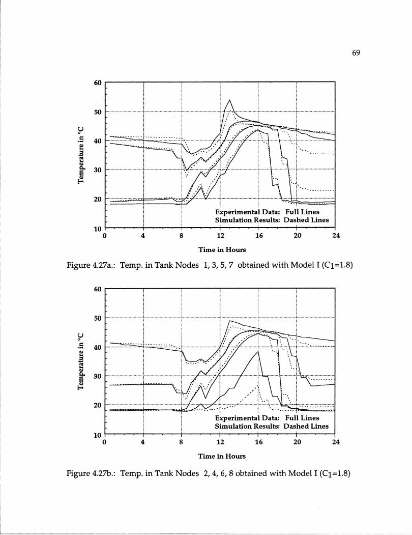
69

50O-

o0 0

40

S30

20

Experimental Data: Full LinesSimulation Results: Dashed Lines

10 .0 4 8 12 16 20 24

Time in Hours

Figure 4.27a.: Temp. in Tank Nodes 1, 3, 5, 7 obtained with Model I (Ci=1.8)

60

40,

530 .........40

0 ........

10 -04 8mna12 16slts 2d 2

Time in Hours

Figure 4.27b.: Temp. in Tank Nodes 2,4, 6,8 obtained with Model I (C1=1.8)

o

0t

60

50

40

30

20

10

Figure 4.28.:

10 11 12 13 14 15 16

Time in Hours

Temperature in Mantle Nodes, obtained with Model I (C1=1.8)

node behave much better and show a reduction of the maximum temperature

deviation of about 30%. As a consequence of the higher heat transfer

coefficient, more energy is transferred from the liquid in the shell to the tank.

Therefore the simulated temperature of the shell outlet is colder and closer to

the measured temperature.

4. 3. 3. Simulation Results with Model II

A simulation using model II has been performed with a heat transfer

correction factor of C1 = 1.8. The temperatures of the tank nodes are displayed

in Figure 4.29a and 4.29b. The corresponding temperatures in the outer tank

are shown in Figure 4.30. The temperatures are displayed for the whole time

of the experiment as model II has the capability of determining the mantle

70

. ..... .... ................ ................ ....

. ... ...... - ' .-" .,-. .-. ... I.............. ....... .................................................... .... ............ ......................

... ....i .. " .-" .A ...... ......... .... .......

.. . .OT- o- ------. . . 6."........". .. .T2- -- - T ......

I

71

60

4 ..

• 4 ............. ' .. .......... -:... .. ............... ....... ........... .... ....... *.. ..............

20......

Experimental Data: Full LinesSimulation Results: Dashed Lines

10 .0 4 8 12 16 20 24

Time in Hours

Figure 4.29a.: Temperatures in Tank Nodes 1, 3, 5, 7 obtained with Model II

60

5 o .................... ............................ ............................. -......... .................... ............................ .............................

40 -

30 ........

20 ......................

10,

0.4 8imu2 1 s 2e 2

Time in Hours

Figure 4.29b.: Temperatures in Tank Nodes 2, 4, 6, 8 obtained with Model II

I

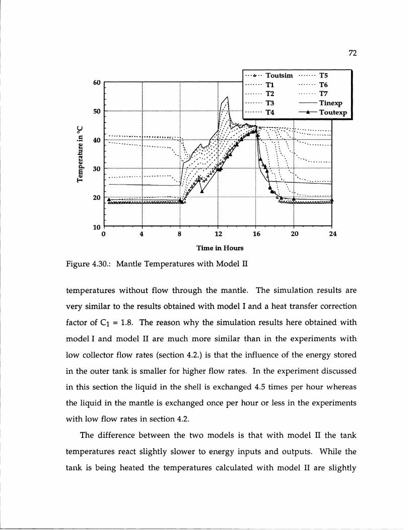
72

60 Ti....... T1.......T6

----T2 ---- T7

T3 Tinexp

0 8wa /l, ,ao .. 12 1 20,, 24 . .......

. ... ........ ....... . .. . ... ... ... ...... . . ...... ... -..... ... ..

50 .........-,Time m,.. Hours , , !3 0 ........................ .......................... " . """ .. .---- P .....................41 . ... ..\- ..... ....... 14 ............................40 . i.i............. .. 0',S"'t",% . -

3 ...... .... .. . . . . . ' , , - , . :

20

Figure 4.30.: Mantle Temperatures with Model II

temperatures without flow through the mantle. The simulation results are

very similar to the results obtained with model I and a heat transfer correction

factor of C1 = 1.8. The reason why the simulation results here obtained with

model I and model II are much more similar than in the experiments with

low collector flow rates (section 4.2.) is that the influence of the energy stored

in the outer tank is smaller for higher flow rates. In the experiment discussed

in this section the liquid in the shell is exchanged 4.5 times per hour whereas

the liquid in the mantle is exchanged once per hour or less in the experiments

with low flow rates in section 4.2.

The difference between the two models is that with modelMoIthe tank

temperatures reacot gtlflowrg theerg insandlh outults.n Wiesthae

tank singeatd the temprtursacuaed with model IIadahettae sligtlyn

73

lower than for model I and during times of draws. During the time when

there is no mass flow through the shell and energy is drawn from the tank,

the tank nodes simulated with model II cool at a slower rate than in model I.

The faster reaction of the tank simulated with model I is caused by the fact that

model I does not account for energy storage in the mantle.

74

5. Investigation of Mantle Heat ExchangerTanks

Computer simulations of energy systems are performed to optimize their

energy yield. In this chapter, yearly simulations of a sample system are

performed to investigate the impact of different parameters on the system's

output. In the first part of this chapter the performance of the mantle heat

exchanger subroutine is analyzed for different parameters. The energy

outputs for the two different models are compared for different collector flow

rates, different loads, and different heat transfer correction factors. In the

second part the system with mantle heat exchanger is compared to a system

with a regular tank and a separate heat exchanger.

5. 1 Base Case System

The base case system is a domestic hot water system with a solar collector and

a hot water storage tank. The collector loop is separated from the storage unit

by a heat exchanger. The system is located in Sacramento, California and has

to meet a hot water load which is varied between 200 liters and 400 liters a day.

The solar collector is of the flat plate type and has an area of 5 in2 . The

75

single glazed collector has a linear efficiency which is defined by FR(To)=0.7

and FRUL=4.17 W/m 2K. The incidence angle modifier constant is b0=0.1. The

liquid in the collector loop is water. The storage tank has a volume of 200

liters. For the simulations it is divided into 10 equal nodes (apart from the

one node simulation of the regular tank). The load requires water at a

temperature of 601C and is supplied by either mixing the water from the tank

with water from the mains if the water from the tank is too hot, or by heating

it with an auxiliary heater if it is colder than 60°C. The 200 liters/day load

profile used is displayed in Figure 5.1. The 400 liter/day and the 600 liter/day

load are obtained by multiplying this load by 2 or 3, respectively. The

performance of the solar system is compared in terms of solar fractions, the

fraction of the total energy required which is supplied by the sun.

25

20 ................ .......................................".......... .................. ..................... ......................

.~15-

15 ....... . ... ...... ..... ., 0

0 4 8 12 16 20 24

Time mn Hours

Figure 5.1.: Load Profile for a Hot Water Consumption of 200 liters/day

76

5. 3. Variation of Parameters

The simulation with model II was chosen as the standard situation for the

parametrical analysis. 150 liters/hour was used as collector flow rate. The

solar fractions for different heat transfer correction factors and for different hot

water consumptions are displayed in Figure 5.2. The hot water loads were

chosen to obtain solar fractions in different regions. For high solar fractions,

different heat transfer coefficients have a relatively small impact on the

system performance. Doubling the heat transfer coefficient results in a only

2.5 % higher solar fraction, halving it causes 5 % lower results. For

intermediate and small solar fractions the differences are larger. Doubling the

heat transfer coefficient there causes an increase in solar fraction of 8 %, to half

it results in a by 12.5 % reduced solar fraction.

To obtain Figure 5.3 the same simulations were run again, but with an

almost doubled collector flow rate of 270 liters/hour. The results for the

different collector flow rates hardly vary. For solar fractions between 30% and

60% they are between 1% and 2% higher when the high flow rate is used

instead of the low flow rate. For the high solar fractions of about 80% the

situation is inverted, and the solar fractions increase with a decrease of the

flow rate.

Model II, the model which does not include the heat storage in the mantle

was simulate for a flow rate of 150 liters/hour. The results of the annual

simulations are displayed in Figure 5.4. The solar fractions are between 2%

and 16% lower for model I compared to the solar fractions obtained with

model II. The reason for that behavior is, that neglecting the energy stored in

the mantle is equivalent to using a smaller storage volume, in this case

77

C11) 0C1 --o~~~~~~~~s ~ ~ ~ .... .... i. ........................ ...! c = I

o 0 ...........0 .8 ... .... .. ................................................

!-i ++ ....... ,'.''o'-'. ...........

0 \ X ........................... .....- ,,.......iii!!i~li

0 . 6 ..... .......... ............ ..

....... 0 .. i Ln!!:~~::::::

0 8- " ... ........................-- ............

..-_ o + .......... = .... ... ............. ..... ..... ..........0 .4.... ..... ............. ...... .

0 .24............. ..

.. ..... .200..4...60 .

Hot Wate Load.........ay

Figur 5.3" Soar Factin fo Modl II nd aCollctorF.owRateof.20./hfo r 3...f........rr...........r

78

1.0......

0.0 -0.

0 ,8 .... ii! ! i!ii!!ii ~ii i i !! ...... ..-... -. ...... '. ..................................................

O .6!::ii~~i!i ~i! !.... ............. ' 4 ..... .......................................:... :.:..., ...................~~~~~............. i !iiii~ii~iii

0 .6 ........... ... ................. i~ii .......... .........., ..............t 0 •4 ii~ii~i!!i!................Cj............................iiiii~~i...... ...................iii~iii

o . 2 ...... ..........

200 400 600

Hot Water Load [liters/day]

Figure 5.4.: Solar Fraction for Model I and a Collector Flow Rate of 150 1/hr

for 3 different correction factors

reduced by approximately 15%. The energy outputs, predicted with model I

are further away from the outputs predicted with model II for small heat

transfer coefficients.

5. 3.. Mantle Heat Exchanger vs. System with Separate Heat

Exchanger

In this section the performance of a tank with a mantle heat exchanger is

compared to a regular tank with a separate heat exchanger. The heat

exchanger effectiveness has been varied in the system having the separate

tank. The values of the heat exchanger effectiveness used in the simulation

o

(U

1.0

0.8

0.6

0.4

0.2

0.0200 400 600

Hot Water Load [liters/day]

Figure 5.5.: Tank with Separate Heat Exchanger and 10 Nodes

0

(U

(U

1.0

0.8

0.6

0.4

0.2

0.0200 400 600

Hot Water Load [liters/day]

Figure 5.6.: Tank with Separate Heat Exchanger and 1 Node

79

80

were set to be 0.3 to represent the lower limit, 0.5 which represents a

commonly used type of heat exchanger and 1.0 to get the upper performance

limit.

The simulation results for a regular tank with the same node

configuration as the mantle heat exchanger tank are displayed in Figure 5.5. If

the results for this regular tank with external heat exchanger are to be

compared to the results from the simulations using the mantle heat

exchanger model II, it is appropriate to relate the regular tank with an

effectiveness of the external heat exchanger eff = 1.0 to the results from

model II with a heat transfer correction factor of C1 = 2. The heat exchanger

effectiveness of eff = 1.0 represents the upper performance limit of the regular

tank system. A heat transfer correction factor of C1 = 2 is in the region where

model II works best. When these two configurations are compared, the mantle

heat exchanger tank performs 3 % better for high solar fractions and almost

equal for low and intermediate solar fractions.

A problem connected with this comparison is that the tank with mantle

heat exchanger has additional storage capacity in the mantle. The total

volume (including mantle) is therefore 230 liters. Yearly simulations for a

regular tank with separate heat exchanger and a storage capacity of 230 liters

have been performed. If the regular system with a 200 liter tank is compared

to the system with the 230 liter tank, the system with the large tank has

between 0.3 % (high solar fractions) and 1.5 % (intermediate and low solar

fractions) higher solar fractions.

If a regular tank is divided into ten nodes an unrealistically high

stratification in the tank to be calculated whereas the simulated high

stratification in a tank with a mantle heat exchanger is not unreasonable as

81

experiments have shown [2]. If the thermal stratification is overpredicted the

simulated value of the solar fraction is also too high. A simulation with ten

nodes therefore yields the upper limit of the performance that can be expected.

The lower limit for the performance of a tank can be obtained by simulating

the tank as fully mixed with only one node. A simulation with only one node

certainly underpredicts the thermal performance of the tank. Yearly

simulations for a tank with one node have been done and the results are

presented in Figure 5.6. The solar fractions are calculated to be between 10%

and 24% lower than for the mantle heat exchanger model.

These results indicate that the thermal performance of a tank with mantle

heat exchanger is better than the thermal performance of a tank with a

separate heat exchanger as the upper performance limit of the tank with a

separate heat exchanger just reaches the performance of a normal mantle heat

exchanger tank.

F

82

6. Conclusion and Recommendations

A simulation model for a hot water storage tank with a built-in mantle heat

exchanger has been developed. Two different approaches have been taken.

One approach treats the flow through the mantle as being at steady state

during the time step and therefore does not take into account the energy

stored in the mantle. In the second modeling approach, the tank is divided

into control volumes for which energy balances are applied. Model II is

therefore capable of accounting for the energy stored in the mantle.

The heat transfer coefficient from the mantle liquid to the heat transfer

wall has been obtained from an empirical correlation. To make the model II

agree with experimental measurements the heat transfer coefficient obtained

by the correlation has to be multiplied by a correction factor of 1.8 for model II.

Model I works best for a correction factor of 1.0.

The predicted performance for the heating experiment with a low flow

rate is reasonable for model II while the error with model I is not acceptable.

For the experiment with draws and for the cooling experiment both models

predict a similar behavior like the real tank, but the calculated temperatures

are relatively far off. For the tank-in-tank experiment both models perform

very well. The only weak spot is the period were draws are extracted, but the

83

flow through the mantle is already shut off. It can be concluded that the

predictions with model I are not sufficiently accurate. The accuracy of the

simulations with model II are satisfactory with the exception of the

experiment with a low mantle flow rate and draws. To be sure that model II

predicts reliable results, it is therefore necessary to further investigate model II

by running more simulations for different experiments.

The attempt to include free convection as a heat transfer mode shows that

it the water in the tank cannot be assumed to be an infinite medium with the

wall being at a constant temperature. A model including free convection

based on these assumptions greatly overpredicts the decay of stratification in

the cooling experiment (section 4. 2. 3). However in the cooling experiment

with only conduction as a heat transfer coefficient the stratification decays too

slow, which indicates that a small amount of free convection actually occurs.

As shown by yearly simulations of a mantle heat exchanger tank and a

tank with separate heat exchanger for similar conditions, the mantle heat

exchanger has a slightly superior thermal performance which is most likely

due to the stratification in this tank.

No satisfactory relations could be found which describe the heat transfer

that occurs in an enclosure like a tank. Further investigations are necessary to

obtain a relation for the Nusselt number for the heat transfer from the mantle

liquid to the wall between mantle and tank, and for the heat transfer from the

wall to the liquid in the tank. However, additional experiments are needed as

there is not enough experimental data available today.

Future improvement of the mantle heat exchanger model should involve

a separate mode for tank-in-tank systems in order to include the larger heat

transfer areas on the tank top and bottom.

84

Appendix A: TRNSYS Component Configuration

PARAMETERS NO. DESCRIPTION

- 3 tank with mantle heat exchanger

- tank volume

Cp - specific heat of fluid in tank

p - density of fluid in tank

environmentUt-env

H or Hi

- loss coefficient from tank to

if > 0 height of node 1if < 0 then all nodes are the same size

and the total tank height is H

if Parameter 6 > 0:

5+i

5+n

- height of ith node

- height of nth node (n < 16)

Parameter for Mantle

last- 9

last- 8

hman distance to top of mantle from bottomof tank

distance to bottom of mantle frombottom of tank

Mode:

V

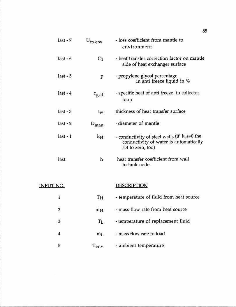
85

last - 7

last- 6

last- 5

last - 4

last- 3

last - 2

last - 1 1<

INPUT NO.

1

2

3

4

5

TH

rfH

TL

nL

Tenv

DESCRIPTION

- temperature of fluid from heat source

- mass flow rate from heat source

- temperature of replacement fluid

- mass flow rate to load

- ambient temperature

Um-e- loss coefficient from mantle to

environment

C1 - heat transfer correction factor on mantleside of heat exchanger surface

p - propylene glycol percentagein anti freeze liquid in %

p,af - specific heat of anti freeze in collector

loop

tw thickness of heat transfer surface

n;n - diameter of mantle

-st - conductivity of steel walls (if kst=O theconductivity of water is automaticallyset to zero, too)

h heat transfer coefficient from wallto tank node

last

c

WDn

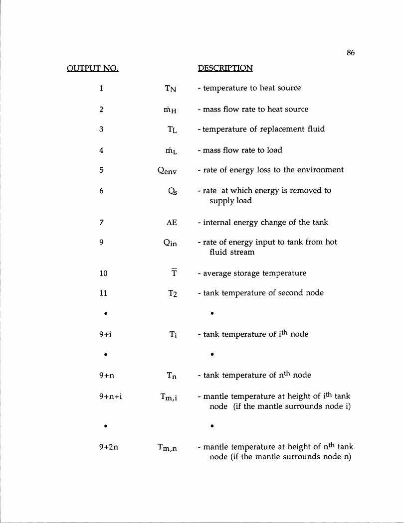
86

OUTPUT NO.

1

2

3

4

5

6

7

9

10

11

9+i

0

9+n

9+n+i

9+2n

TN

rnH

TL

rmtL

Qenv

Qs

AE

Qin

T

T2

DESCRIPTION

- temperature to heat source

- mass flow rate to heat source

- temperature of replacement fluid

- mass flow rate to load

- rate of energy loss to the environment

- rate at which energy is removed tosupply load

- internal energy change of the tank

- rate of energy input to tank from hotfluid stream

- average storage temperature

- tank temperature of second node

Ti - tank temperature of ith node

Tn

Tm,i

Tm,n

- tank temperature of nth node

- mantle temperature at height of ith tank

node (if the mantle surrounds node i)

0

- mantle temperature at height of nth tanknode (if the mantle surrounds node n)

DERIVATIVE NO.

1

i

n

DESCRIPTION

Ti - initial temperature of top tank node

Ti - initial temperature of ith tank node

Tn - initial temperature of nth tank node

Initial Temperatures for the Mantle only for Model II:

n+i Tm,i initial mantle temperature at height ofith tank node (if no mantle at node i:Tm,i=O)

2n Tm,n - initial mantle temperature at height ofnth tank node (if no mantle at node n:Tm,n=O)

87

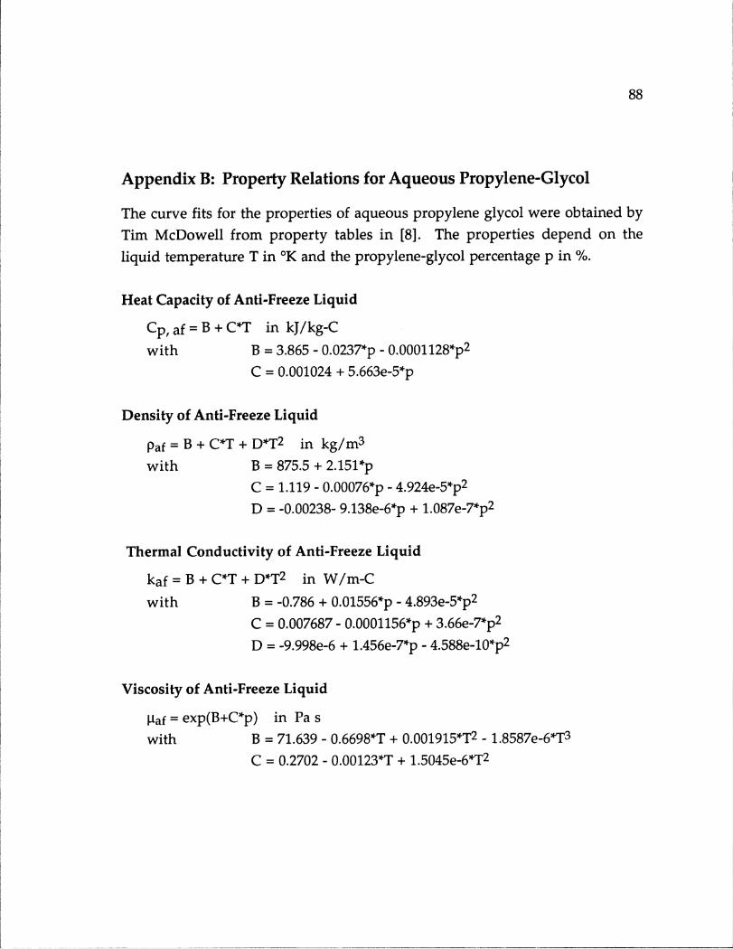
88

Appendix B: Property Relations for Aqueous Propylene-Glycol

The curve fits for the properties of aqueous propylene glycol were obtained by

Tim McDowell from property tables in [8]. The properties depend on the

liquid temperature T in 'K and the propylene-glycol percentage p in %.

Heat Capacity of Anti-Freeze Liquid

Cp, af = B + C*T in kJ/kg-C

with B = 3.865 - 0.0237"p - 0.0001128*p 2

C = 0.001024 + 5.663e-5*p

Density of Anti-Freeze Liquid

Paf = B + C*T + D*T2 in kg/m3

with B = 875.5 + 2.151"p

C = 1.119 - 0.000 7 6 "p - 4.924e-5*p2

D = -0.00238- 9.138e-6*p + 1.087e-7*p2

Thermal Conductivity of Anti-Freeze Liquid

kaf = B + C*T + D*T2 in W/m-C

with B = -0.786 + 0.01556"p - 4.893e-5*p 2

C = 0.007687 - 0.000115 6 "p + 3.66e-7*p2

D = -9.998e-6 + 1.456e-7*p - 4.588e-10*p 2

Viscosity of Anti-Freeze Liquid

9af = exp(B+C*p) in Pa s

with B = 71.639 - 0.6698*T + 0.001915*T2 - 1.8587e-6*T3

C = 0.2702 - 0.00123*T + 1.5045e-6*T2

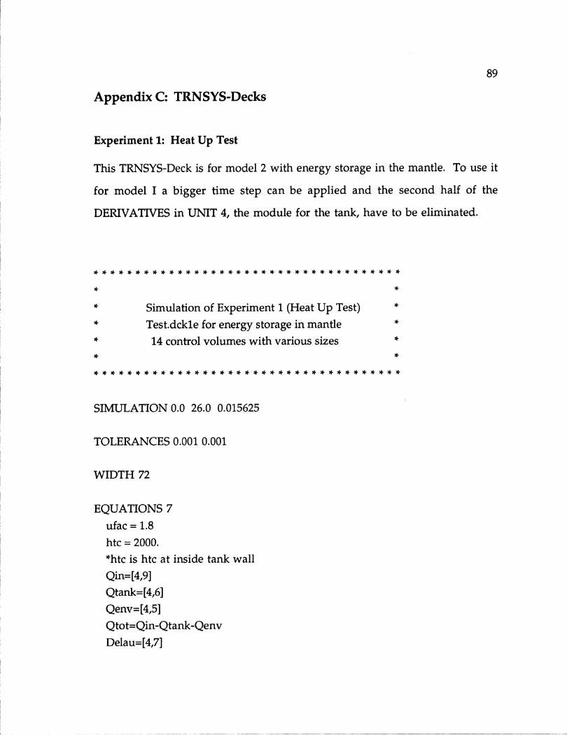
89

Appendix C: TRNSYS-Decks

Experiment 1: Heat Up Test

This TRNSYS-Deck is for model 2 with energy storage in the mantle. To use it

for model I a bigger time step can be applied and the second half of the

DERIVATIVES in UNIT 4, the module for the tank, have to be eliminated.

Simulation of Experiment 1 (Heat Up Test) *

Test.dckle for energy storage in mantle *

14 control volumes with various sizes *

SIMULATION 0.0 26.0 0.015625

TOLERANCES 0.001 0.001

WIDTH 72

EQUATIONS 7

ufac = 1.8

htc = 2000.* htc is htc at inside tank wall

Qin=[4,9]

Qtank=[4,6]

Qenv=[4,51

Qtot=Qin-Qtank-QenvDelau=[4,71

90

UNIT 4 TYPE 4 storage tank with mantle heat exchanger

PARAMETERS 293.0 0.197 4.186 1000. 3.204*mode vol cp rho utank

0.092 0.05 0.15 0.05 0.15 0.05 0.13 0.05 0.16 0.05 0.14 0.05 0.05 0.04

*hl h2 h3 h4 h5 h6 h7 h8 h9 hiG hil h12 h13 h14

1.013 0.098 3.204 Ufac 0. 4.186 0.005 0.504216.htc

*hman eman uman Ufac perc cph tht dman kst htc

INPUTS 514,1 15,1 0,0 0,0 0,030.0 22.2 15 0.0 20.4*Ts mdoth Tl mdotl Tenv

DERIVATIVES 2829.5 29.5 29.5 29.5 29.5 29.5 29.5

29.5 29.3 29.2 29.0 28.7 28.2 27.7

0.0 0.0 29.5 29.5 29.5 29.5 29.5

29.5 29.3 29.2 29.0 28.7 0.0 0.0

UNIT 14 TYPE 14 mantle inlet temperaturePARAMETERS 16

0.30. 0.2 30. 0.5 47. 1. 49.2 2.49.3 9.49.3 11. 49.4 26. 49.4

UNIT 15 TYPE 14 mantle flow ratePARAMETERS 12

0. 22.2 .5 25.8 1.28.2 3. 28.8 6. 31.2 26.31.2

91

UNIT 25 TYPE 25 printerPARAMETERS 4

0.5 0. 26. 10INPUTS 8

4,11 4,13 4,15 4,17 4,19 4,21 4,23 4,1tl t2 t3 t4 t5 t6 t7 Tmout

UNIT 27 TYPE 25 printer for mantle temperaturesPARAMETERS 4

0.25 0. 26. 11INPUTS 8

4,25 4,27 4,29 4,31 4,33 4,35 4,37 4,1

tml tm2 tm3 tm4 tm5 tm6 tm7 Tmout

UNIT 26 TYPE 25 printer for energyPARAMETERS 4

1. 0. 26. 12INPUTS 5

Qin Qtank Qenv Qtot DelauQin Qtank Qenv Qtot Delau

END.

Experiment 2: Test with Draws

This TRNSYS-Deck is for model 2 with energy storage in the mantle. To use it

for model one a bigger time step can be applied and the second half of the

DERIVATIVES in UNIT 4, the modul for the tank, have to be eliminated.

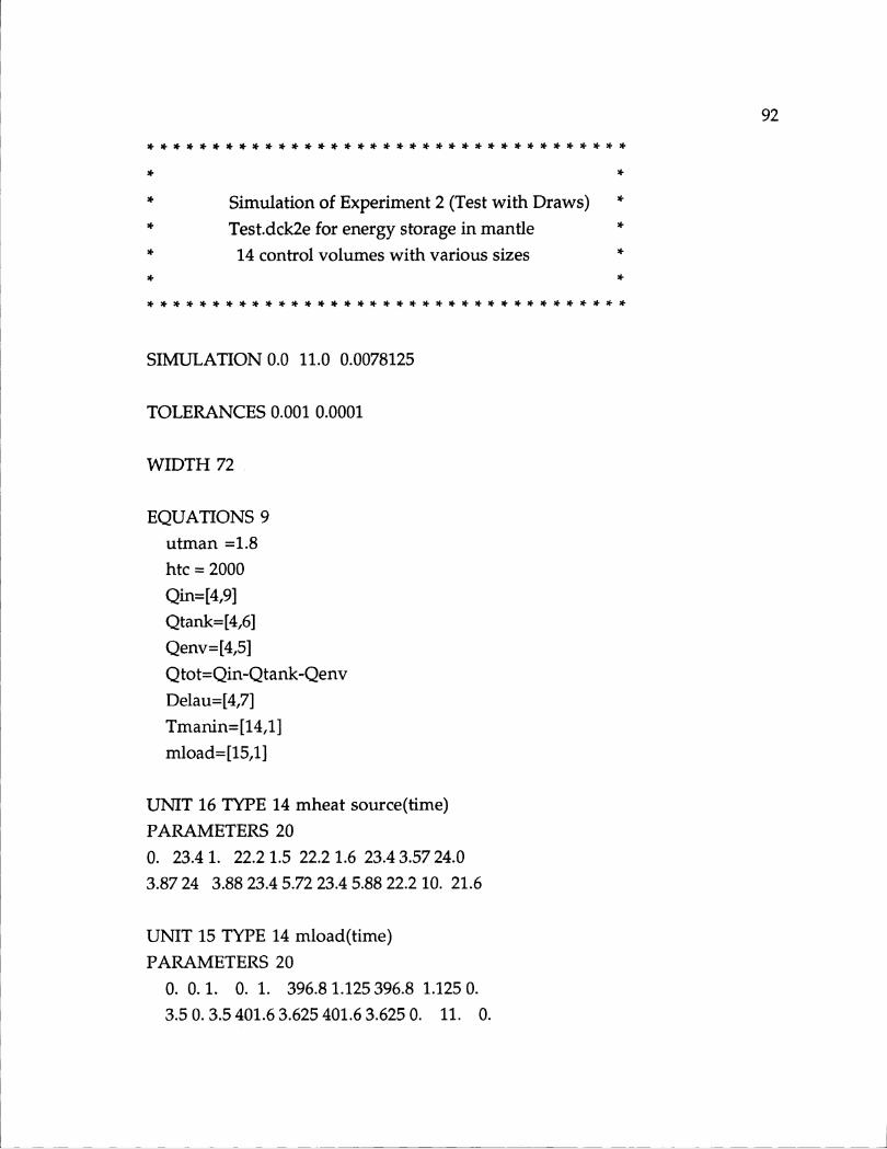
92

Simulation of Experiment 2 (Test with Draws) *

Test.dck2e for energy storage in mantle *

14 control volumes with various sizes *

SIMULATION 0.0 11.0 0.0078125

TOLERANCES 0.001 0.0001

WIDTH 72

EQUATIONS 9utman =1.8htc = 2000

Qin=[4,9]Qtank=[4,6]Qenv=[4,5]

Qtot=Qin-Qtank-QenvDelau=[4,7]

Tmanin=[14,1]mload=[15,1]

UNIT 16 TYPE 14 mheat source(time)PARAMETERS 20

0. 23.4 1. 22.2 1.5 22.2 1.6 23.4 3.57 24.03.87 24 3.88 23.4 5.72 23.4 5.88 22.2 10. 21.6

UNIT 15 TYPE 14 mload(time)PARAMETERS 20

0. 0. 1. 0. 1. 396.8 1.125396.8 1.125 0.

3.5 0. 3.5 401.6 3.625 401.6 3.625 0. 11. 0.

93

UNIT 14 TYPE 14 Tmanin(time)

PARAMETERS 48

0. 29.5 1.0 29.7 1.6 29.7 1.62 34.6 1.78 59.4

1.95 67.0 2.12 69.0 2.28 69.7 2.95 69.9 3.28 70.1

5.72 70.1 5.88 69.1 6.05 56.9 6.22 45. 6.38 37.5

6.55 32.7 6.72 30.9 6.88 30.3 7.05 30.0 7.72 29.9

8.05 29.8 9.05 29.7 10.05 29.7 11.0 29.5

UNIT 4 TYPE 4 tank with mantle heat exchanger

PARAMETERS 29

3 .0 0.197 4.186 1000. 3.204 0.092 0.05 0.15 0.05*mode vol cp rho utank hl h2 h3 h4

0.15 0.05 0.13 0.05 0.16 0.05 0.14 0.05 0.05 0.04*h5 h6 h7 h8 h9 hlO hil h12 h13 h14

1.013 0.098 3.204 Utman 0. 4.186 0.005 0.504 216 htc*hman eman uman Utman perc cph tht dmankst htc

INPUTS 5

Tmanin 16,1 0,0 mload 0,0

29.5 23.4 14.2 0.0 21.5

* Ts mdoth Tl mload Tenv

DERIVATIVES 28

19.1 19.1 18.4 17.8 17.3 16.8 16.8

16.7 16.6 16.5 16.6 16.7 16.6 16.5

0.0 0.0 18.4 17.8 17.3 16.8 16.8

16.7 16.6 16.5 16.6 16.7 0.0 0.0

UNIT 25 TYPE 25 printer

PARAMETERS 4

0.125 0. 26. 10

INPUTS 84,11 4,13 4,15 4,17 4,19 4,21 4,23 4,1

ti t2 t3 t4 t5 t6 t7 Tmout

94

UNIT 27 TYPE 25 printer for mantle temperatures

PARAMETERS 4

0.25 0. 26. 11

INPUTS 8

4,25 4,27 4,29 4,31 4,33 4,35 4,37 4,1

tml tm2 tm3 tm4 tm5 tm6 tm7 Tmout

UNIT 26 TYPE 25 printer for energy

PARAMETERS 4

1. 0. 26. 12

INPUTS 5

Qin Qtank Qenv Qtot DelauQin Qtank Qenv Qtot Delau

END.

Experiment 3: Cool Down Test

This TRNSYS-Deck is for model 2 with energy storage in the mantle. To use it

for model one a bigger time step can be applied and the second half of the

DERIVATIVES in UNIT 4, the modul for the tank, have to be eliminated.

Simulation of Experiment 3 (Cool Down Test) *

Test.dck3e for energy storage in mantle *

14 control volumes with various sizes *

SIMULATION 0.0 25.0 0.0625

95

TOLERANCES 0.001 0.001

WIDTH 72

EQUATIONS 7

utman = 1.8

htc = 2000

Qin=[4,9]Qtank=[4,6]

Qenv=[4,5]

Qtot=Qin-Qtank-QenvDelau=[4,7]

UNIT 4 TYPE 4 tank with mantle heat exchanger

PARAMETERS 293.0 0.197 4.186 1000. 3.204 0.092 0.05 0.15 0.05*mode vol cp rho utank hl h2 h3 h4

0.15 0.05 0.13 0.05 0.16 0.05 0.14 0.05 0.05 0.04

*h5 h6 h7 h8 h9 hl0 hil h12 h13 h14

1.013 0.098 3.204 Utman 0. 4.186 0.005 0.504 216 htc*hman eman uman Utman perc cph tht dmankst htc

INPUTS 5Tmanin 16,1 0,0 mload 0,029.5 23.4 14.2 0.0 21.5* Ts mdoth Tl mload Tenv

DERIVATIVES 2848.0 48.0 47.9 47.8 46.0 44.3 33.6

22.9 21.2 19.4 19.3 19.3 19.2 19.1

48.0 48.0 47.9 47.8 46.0 44.3 33.6

22.9 21.2 19.4 19.3 19.3 19.2 19.1

UNIT 25 TYPE 25 printer

PARAMETERS 4

0.125 0. 26. 10

96

INPUTS 8

4,11 4,13 4,15 4,17 4,19 4,21 4,23 4,1

tl t2 t3 t4 t5 t6 t7 Tmout

UNIT 27 TYPE 25 printer for mantle temperatures

PARAMETERS 4

0.25 0. 26. 11

INPUTS 8

4,25 4,27 4,29 4,31 4,33 4,35 4,37 4,1

tml tm2 tm3 tm4 tm5 tm6 tm7 Tmout

UNIT 26 TYPE 25 printer for energy

PARAMETERS 4

1. 0. 26. 12

INPUTS 5

Qin Qtank Qenv Qtot DelauQin Qtank Qenv Qtot Delau

END.

97

Appendix D: FORTRAN Source Code of Model II

SUBROUTINE TYPE4(TIME,XIN,OUT,T, DTDT, PAR, INFO)

C THIS ROUTINE SIMULATES A STRATIFIED STORAGE TANK CONSISTING OF NEQ

C FULLY MIXED SECTIONS, THE VALUE OF NEQ BEING CHOSEN BY THE USER.

C REFERENCE 'EXPERIMENTAL AND SIMULATED PERFORMANCE OF A CLOSED

C LOOP SOLAR WATER HEATING SYSTEM', BY P.I.COOPER, S.A.KLEIN,

C AND C.W.S.DIXON PRESENTED AT THE ISES MEETING IN AUGUST,1975

C THIS SUBROUTINE WAS CHANGED TO MODEL A TANK WITH A MANTLE HEAT

C EXCHANGER. THE MANTLE IS DIVIDED UP IN CONTROL VOLUMES, ON WHICH

C ENERGYBALANCES ARE APPLIED.

INTEGER FINAL,DIRECT, AVG,OLD,MANP,AUXP, INV, NMANIN, NMANOUT,

+ FLAG

REAL MSCP, MCPN

REAL HMAN,UMANKTMAN,RHOH,CPH,THT,DMAN,AMAN,ALOSS, UTMAN,

+ ACTHIGHEXCHIGHCONSTFLWSSQENVTSPECTIMEDELAU,

+ UTMANX,EMAN,XUT,KAOXH20(15),KAOXST(15),HTCX,DELX,KAF,

+ KH20,KST,KAOX(15),REY,PR,DH,X1,X2,HTC(15),HTC1(15),MY,

+ DELAUMAN, TMANAV,TMANAV2,AAMAN, BBMAN,ACROSSMAN,TMANI,

+ TMANF,T2,T1,TL, PERCCPDF, DENSITY,THCOND,VISC

DIMENSION T(30),DTDT(30),XIN(10),OUT(40),PAR(40),INFO(10)

DIMENSION U(16),V(16),QB(16),H(15)

COMMON/SIM/TIMEO,TFINAL,DELT

COMMON/STORE /NSTORE,IAV,S(5000)

DATA NSTK/5/,QB/16*0.0/,PI/3.1415193/,LOCT/O/

EXTERNAL CPDF, DENSITY,THCOND,VISCC

IF (INFO(7).GE.O) GO TO 10

C FIRST CALL OF SIMULATION

C SPECIFY SIZE OF OUTPUT ARRAY

INFO(6) =40

NI=5

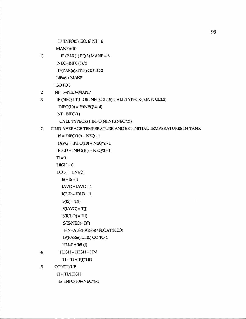
98

IF (INFO(3).EQ. 6) NI = 6

MANP =10

C IF (PAR(1).EQ.3) MANP = 8

NEQ=INFO(5)/2

IF(PAR(6).GT.O.) GO TO 2

NP=6 + MANP

GOT03

2 NP=5+NEQ+MANP

3 IF (NEQ.LT.1 .OR. NEQ.GT.15) CALL TYPECK(5,INFO,0,0,0)

INFO(10) = 2*(NEQ*4+4)

NP=INFO(4)

CALL TYPECK(1,INFONINP,(NEQ*2))

C FIND AVERAGE TEMPERATURE AND SET INITIAL TEMPERATURES IN TANK

IS = INFO(10) + NEQ- 1

IAVG = INFO(10) + NEQ*2- 1

IOLD = INFO(10) + NEQ*3- 1

TI-= 0.

HIGH = 0.

DO 5 J = 1,NEQ

IS=IS+1

IAVG=IAVG + 1

IOLD = IOLD + 1

S(IS) = T(J)

S(IAVG) = T(J)

S(IOLD) = T(J)

S(IS-NEQ)=T(J)

HN=ABS(PAR(6))/FLOAT(NEQ)

IF(PAR(6).LT.0.) GO TO 4

HN=PAR(5+J)

4 HIGH = HIGH + HNTI = TI + T(J)*HN

5 CONTINUE

TI = TI/HIGH

IS=INFO(10)+NEQ*4-1

99

S(IS+1)=TI

C

C FIND NODE NUMBER OF MANTLE TOP AND BOTTOM (NMANIN,NMANOUT)

IND=1

IF(PAR(6).GT.0.) IND=NEQ

HMAN= PAR(5+IND+I)

EMAN= PAR(5+IND+2)

FLAG--0

ACIH[GH=HIGH

DO 6J=1,NEQ

HN=ABS(PAR(6))/FLOAT(NEQ)

IF(PAR(6).LT.O.) GO TO 7

HN=PAR(5+J)

7 ACTHIGH = ACTHIGH -HN

IF ((ACTHIGH.LT.HMAN).AND.(FLAG.LT.1.)) THEN

FLAG=2

NMANIN=J

ENDIF

IF ((ACTHIGH.LE.EMAN).AND.(FLAG.LT.3.)) THEN

FLAG=4

NMANOUT=J

ENDIF

6 CONTINUE

C READ IN MANTLE INITIAL TEMPERATURES

IS = INFO(10)+ NEQ*4+4 + NEQ- 1

IAVG = INFO(10)+ NEQ*4+4 + NEQ*2- 1

IOLD = INFO(10)+ NEQ*4+4 + NEQ*3- 1

C DO 8 J = NMANINNMANOUT

DO 8 J = 1,NEQ15=15+1

IAVG =IAVG+ 1

IOLD = IOLD + 1

S(IS) = T(J+NEQ)

100

S(IAVG) = T(J+NEQ)

S(IOLD) = T(J+NEQ)

S(IS-NEQ)=T(J+NEQ)

8 CONTINUE

IUNIT=O

C

C END OF PART FOR 1ST SUBROUTINE CALL

C

C

C SET LOCAL VARIABLES TO PARAMETER VALUES.

C PARAMETERS ARE READ IN ONLY THE FIRST TIME, OR AT EVERY CALL IF THERE

C IS MORE THAN ONE TYPE4 SPECIFIED IN THE DECK

10 IF (INFO(1).EQ.IUNIT) GO TO 30

IUN1T=INFO(1)

NEQ = INFO(5)/2

XNEQ = FLOAT(NEQ)

MODE=INT(PAR(1)+0.1)

VOL = PAR(2)

CPF=PAR(3)

RHOF=PAR(4)

ULOSS=PAR(5)

IND=1

IF(PAR(6).GT.0.) IND=NEQ

C

C ADDITIONAL PARAMETERS FOR MANTLE HEAT EXCHANGER MODEL

IF (MANP .EQ. 10) THEN

HMAN= PAR(5+IND +1)

EMAN= PAR(5+IND +2)

UMAN= PAR(5+IND +3)

UTMAN=PAR(5+IND +4)PERC= PAR(5+IND 5)

CPH= PAR(5+IND +6)

THT= PAR(5+IND +7)

DMAN= PAR(5+IND +8)

101

KST= PAR(5+IND +9)

HTCX= PAR(5+IND +10)

ACROSSMAN=PI/4.*DMAN**2 - VOL/HIGH

DH= DMAN - 2*(THT+ (VOL/PI/HIGH)**0.5)

ENDIF

INIT = INFO(10)- 1

FINAL = INIT + NEQ

AVG = FINAL + NEQ

OLD = AVG + NEQ

IS--OLD+NEQ

UAE=ULOSS*VOL/HIGH

PER=(4.*PI*VOL/HIGH)**0.5

30 CONTINUEC

C SET INPUTS (EVERY CALL OF SUBROUTINE)

TIN=XIN(1)

FLWSS=XIN(2)

TL=XIN(3)

FLWLL=XIN(4)

TENV=XIN(5)

FLWS=FLWSS*CPH

FLWL=FLWLL*CPF

C

C CORRECT FOR TEMP. INVERSIONS ONLY ONCE PER TIMESTEP

1000 IF (INFO(7).GT.0) GO TO 1060

INV--0

TMIX=S(FINAL+NEQ)

HMIX=H(NEQ)

FLAG--0

C FLAG = NUMBER OF NODES IN MIX - 1DO 1005 JJ=NEQ-1,1,-1

IF(S(FINAL+JJ).LT.TMIX) THEN

FLAG =FLAG+I

TMIX= (TMIX*HMIX +S(FINAL +JJ)*H(JJ)) /(HMIX +H(JJ))

102

HMIX=HMIX+H(JJ)

IF ((S(FINAL+JJ-1).GE.TMIX).OR.(JJ.EQ.1)) THEN

DO 1007 KK=jj,(JJ+FLAG)

S(FINAL+KK)=TMIX1007 CONTINUE

FLAG--0

TMIX=S(FINAL+JJ)

HMIX=H(OJ)

ENDIF

ELSE

HMIX=H(JJ)

TMIX=S(FINAL+JJ)

ENDIF

1005 CONTINUE

C

C CHECK FOR INVERSIONS DUE TO MIXING, REPEAT INVERSION ALGORITHM

C IF THERE ARE STILL INVERSIONS

FLAG--0

DO 1008 JJ=NEQ-I,1,-1

IF(S(FINAL+JJ).LT.S(FINAL+JJ+1)) FLAG =1

1008 CONTINUE

IF (FLAG.EQ.1) GOTO 1000

MSCP=VOL*DENSITY(PERC,40)*CPF

CDO 1050 K = 1,NEQ

KI=INlT+K

KF =FINAL+ K

C RESET T INITIAL FOR NEW TIME STEP WITH T FINAL FROM OLD TIME STEP

S(KI+NEQ*4+4)=S(KF+NEQ*4+4)

1050 S(KI) = S(KF)

1060 CONTINUE

C

C CALCULATION OF TEMPERATURES IN ALL TANK AND MANTLE NODES

ACTHIGH=HIGH

103

QENV=0.

DELAU--0.

DELAUMAN--0.

DO 1900 N=1,NEQ

NODE =N

C ENTERING FLOWSTREAMS TO TANK

TI=S(AVG+NODE)

IF (NODE .LT.NEQ) THEN

T2 = S(AVG+NODE+I)

ELSE

T2=TL

ENDIF

C

C ENTERING FLOWSTREAMS TO MANTLE

IF ((N.GE.NMANIN).AND.(N.LE.NMANOUT)) THEN

TMANAV=S(4+4*NEQ + AVG + NODE)

IF (NODE .EQ. NMANIN) THEN

TMANAV2 = TIN

ELSE

TMANAV2 = S(4+4*NEQ + AVG + NODE -1)

ENDIF

ELSE

TMANAV=0.

ENDIF

C

C AREA FOR HEAT EXCHANGE WITH MANTLE AND/OR ENVIRONMENT

AMAN=0.

ALOSS=0.

EXCHIGH=0.

IF (N.LT.NMANIN) THENALOSS=PER*H(NODE)

EXCHIGH=0.

ELSE

IF ((N.GT.NMANIN).AND.(N.LT.NMANOUT)) THEN

104

AMAN=PER*H(NODE)

EXCHIGH=H(NODE)

ELSE

C IF BEGINNING OR END OF MANTLE CUTS A NODE

IF (N.EQ.NMANIN) THEN

EXCHIGH= HMAN - ACTHIGH + H(NODE)

ENDIF

IF (N.EQ.NMANOUT) THEN

EXCHIGH=-(EMAN-ACTHIGH)

ENDIF

ALOSS=PER*(H(NODE)-EXCHIGH)

AMAN=PER*EXCHIGH

ENDIF

ENDIF

C

C HEAT TRANSFER COEFFICIENT OF TOP AND BOTTOM CAN BE CHANGED

C BY INCLUDING THE FACTORS

IF (NODE.EQ.1) ALOSS=ALOSS+ VOL/HIGH

C + *1.79/0.89

IF (NEQ.EQ.NODE)ALOSS=ALOSS+VOL/HIGH

C + *2.97/0.89

C

C CALCULATION OF MANTLE FLUID TEMPERATURE REGARDING LOSSES TO ENV.

IF (EXCHIGH .GT. 0.) THEN

KAF=THCOND(PERC,TMANAV)*3.6

MY=VISC(PERC,TMANAV)*3600

PR=MY*CPDF(PERC,TMANAV)*1000/KAF*3.6/3600

IF (INFO(7).LT.0.) THEN

WRITE (17,*)'DH,MY,FLWSS,(DMAN**2-(DMAN-DH)**2)'WRITE (17,*)DH,MY,FLWSS,(DMAN**2-(DMAN-DH)**2)

ENDIF

REY=DH /MY* FLWSS /(PI /4.*(DMAN **2-(DMAN- DH)**2 ))

X1 =HMAN-AC1I-IIGH

105

X2=HMAN- (ACTHIGH-H(N))

IF (X1.LE.O.) X1=0.2/0.93*X2

C LOCAL HEAT TRANSFER COEFFICIENT AT INSIDE OF TANK

HTC(N)=UTMAN*KAF/DH*(

+ (4.9+0.0606*(REY*PR/X2*DH)**(1.2)/

+ (1.+0.0909*(REY*PR/X2*DH)**(0.7)*PR**0.17))*X2 -

+ (4.9+0.0606*(REY*PR/X1*DH)**(1.2)/

+ (1.+0.0909*(REY*PR/XI*DH)**(0.7)*PR**0.17))*X1)/(X2-X1)

UTMANX=1./(1./HTCX + 1./HTC(N))

C

ENDIF

C

C ---- CALC.--OF---CONDUCTION--PARAMETERS ----------------

IF (INFO(7).EQ.-1) THEN

IF (KST.EQ.0) THEN

KAOX(NX)=0.

ELSE

KH20=0.63*3.6

DO 1070 NX=1,(NEQ-1)

IF (HTCX.GT.0) HTC(NX)=HTCX

DELX=(H(NX)+H(NX+1))/2.

KAOXH20(NX)=VOL/HIGH*KH20/DELX

KAOXST(NX)=./((2*DELX/HTC(NX)/H(NX)/H(NX+1)/PER )+

+

(DELX/THT/PER/KST))

KAOX(NX)=KAOXH20(NX)+KAOXST(NX)

1070 CONTINUE

KAOX(O)=0.

KAOX(NEQ)=0.

ENDIF

C

MCPN= MSCP*H(NODE) /HIGH

C

C SOLVE DIFFERENTIAL EQUATION FOR TANK NODE TEMPERATURE

106

KI=INIT + NODE

KF = FINAL + NODE

KAVG = AVG + NODE

AA = -(FLWL + UTMANX*AMAN + ULOSS*ALOSS +

+ KAOX(N) + KAOX(N-1))/MCPN

BB = +(FLWL*T2 + UTMANX*AMAN*TMANAV +

+ ULOSS*ALOSS*TENV+

+ KAOX(N)*S(KAVG+1) + KAOX(N-1)*S(KAVG-1))/MCPN

TI = S(KI)

CALL DIFFEQ(TIMEAABBTITFTAVG)

S(KF) = TF

S(KAVG) = TAVG

C

C SOLVE DIFFERENTIAL EQUATION FOR MANTLE NODE TEMPERATURE

IF (EXCHIGH.GT.O.)THEN

RHOH=DENSITY(PERC,TMANAV)

AAMAN = - (FLWS + UMAN*DMAN*PI*EXCHIGH

+ + UTMANX*PER*EXCHIGH)/

+ (RHOH*ACROSSMAN*CPH*EXCHIGH)

BBMAN = (FLWS*TMANAV2 + UMAN*DMAN*PI*EXCHIGH*TENV

+ + UTMANX*PER*EXCHIGH*TAVG)/

+ (RHOH*ACROSSMAN*CPH*EXCHIGH)

TMANI = S(NEQ*4+4+KI)

CALL DIFFEQ(TIMEAAMANBBMANTMANITMANFTMANAV)

S(NEQ*4+4+KF) = TMANF

S(NEQ*4+4+KAVG) = TMANAV

C

C INTERNAL ENERGY CHANGE IN THE MANTLE

DELAUMAN=DELAUMAN+RHOH*ACROSSMAN*CPH*EXCHIGH*

+ (TMANF-TMANI)/(DELT)ENDIF

C

C ENERGY LOSS FROM TANK

QENV=QENV + ALOSS*ULOSS*(TAVG-TENV)+

107

+ AMAN/PER*PI*DMAN*UMAN*(TMANAV-TENV)

C

C INTERNAL ENERGY CHANGE

DELAU=DELAU+MSCP*H(NODE)/HIGH*(TF-TI)/(DELT)

c

ACTHIGH=ACTHIGH-H(NODE)

1900 CONTINUE

300 TF=0.

DO310 K = 1,NEQ

KI= K + INIT

KF=K+ FINAL

KAVG = K + AVG

KOLD = K + OLD

S(KOLD) = S(KAVG)

TF =TF + S(KF)*H(K)

UA = ULOSS*PER*H(K)

IF(K.EQ.1 .OR. K.EQ.NEQ) UA = UA + UAE

UAFI=O.

DTDT(K) = (S(KF) - S(KI))/DELT

310 CONTINUE

TF = TF/HIGH

320 QTANK = FLWL*(S(AVG+I) - TL)

QIN=FLWSS*CPH*(TIN-S(AVG + NEQ*4+4 + NMANOUT))

QTOT=QIN-QTANK-QENV-DELAUMAN

C

C SET OUTPUTS

OUT(1)=S(AVG+NEQ)

IF (MODE .EQ. 3) OUT(1)=S(AVG + NEQ*4+4 + NMANOUT)

OUT(2)=FLWSS

OUT(3)=S(AVG+1)OUT(4)=FLWLL

OUT(5)=QENV

OUT(6)=QTANK

OUT(7)=DELAU

108

OUT(8)=QBTOT

OUT(9)=QIN

OUT(10)=TF

N=MINO(12,NEQ-1)

IF(N.LT.2) RETURN

DO 350 I=2,NEQ

OUT(9+I)=S(AVG+I)

350 OUT(9+I+NEQ)=S(AVG + NEQ*4+4 + I)

OUT(9+NEQ+1)=S(AVG + NEQ*4+4 + 1)

RETURN

END

C FUNCTION FOR PROPYLENE-GLYCOL PROPERTIES

FUNCTION CPDF(PERCENT,T1)

REAL T,T1,PERCENT,B,C,CPDF

T=T1+273.15

B = 3.865 - 0.0237*PERCENT -0.0001128*PERCENP'*2

C = 0.001024 + 5.663E-5*PERCENT

CPDF = B + C*T

C {KJ/KG-C}

RETURN

END

FUNCTION DENSITY(PERCENTT1)

REAL T,T1,PERCENTB,C,D,DENSITY

T=T1+273.15

B = 875.5 + 2.151*PERCENT

C = 1.119 -0.00076*PERCENT -4.924E-5*PERCENT**2

D = -0.00238- 9.138E-6*PERCENT + 1.087E-7*PERCENT**2DENSITY =B +C*T +D'**2

C {KG/MA3}

RETURN

END

109

FUNCTION THCOND(PERCENT,T1)

REAL T,T1,PERCENT, B,C,D,THCOND

T=T1+273.15

B = -0.786 + 0.01556*PERCENT - 4.893E-5*PERCENT**2

C = 0.007687 - 0.0001156*PERCENT + 3.66E-7*PERCENT**2

D = -9.998E-6 + 1.456E-7*PERCENT -4.588E-10*PERCENT**2

THCOND = B + C*T + D'T**2

C IW/M-C}

RETURN

END

FUNCTION VISC(PERCENT, T1)

REAL T, T1,PERCENT,B,C,VISC

T=T1+273.15

B = 71.639 -0.6698*T + 0.001915**2 - 1.8587E-6*T**3

C = 0.2702 - 0.00123*T + 1.5045E-6*P*2

VISC = EXP(B+C*PERCENT)

C IPA S)

RETURN

END

110

References

[1] Furbo, S. Berg, P., Calculation of the Thermal Performance of

Small Hot Water Solar Heating Systems using Low Flow

Operation, Thermal Insulation Laboratory, Technical University of

Denmark, January 1992

[2] Fanney, A.H., Klein, S. A., "Performance of Solar Domestic Hot

Water Systems at the National Bureau of Standards -Measurements and Predictions", Journal of Solar Energy

Engineering, Vol.105, August 1983

[3] Incopera, F. P., DeWitt, D. P., Introduction to Heat Transfer, Second

Edition, John Wiley & Sons, Inc., 1990

[4] TRNSYS, Version 13.1, Solar Energy Laboratory, University of

Wisconsin, Madison, September 1990

[5] J. A. Duffie, W. A. Beckman, Solar Engineering of Thermal

Processes, Second Edition, John Wiley & Sons, Inc., 1991

[6] WATSUN-manual, Watsun Simulation Laboratory, University of

Waterloo, Ontario, Canada

111

[7] Mercer, W. E., Pearce, W. M., and Hitckcock, J. E., "Laminar Forced

Convection in the Entrance Region Between Parallel Flat Plates",

Trans.ASME, J. Heat Transfer, 89,251 (1967),

[8] Dowfrost, Engineering and Operation Guide for Dowfrost and

Dowfrost HD Inhibited Propylene Glycol-based Heat Transfer

Fluids, Form No. 180-1286-1190 AMS, Nov 1990