1/34

Simulation of Electromagnetic Fields: The Finite-Difference Time-Domain (FDTD)

Method and Its Applications

Veysel Demir, Ph.D.demir@ceet.niu.edu

Department of Electrical Engineering, Northern Illinois University, DeKalb, IL 60115

2/34

Bachelor of Science, Electrical and Electronics Engineering, Middle East Technical University, Ankara, Turkey, 1997.

System Analyst and Programmer, Pamukbank, Software Development Department, Istanbul, Turkey, July 1997 – August 2000.

Master of Science, Electrical Engineering, Syracuse University, Syracuse, NY, 2002.

Doctor of Philosophy, Electrical Engineering, Syracuse University, Syracuse, NY, 2004.

Research Assistant, Sonnet Software, Inc. Liverpool, NY, August 2000 – July 2004.

Visiting research scholar, University of Mississippi, Electrical Engineering Department, University, MS, July 2004 – Present.

Assistant Professor, Department of Electrical Engineering, Northern Illinois University, DeKalb,IL, August 2007 – present

Veysel Demir

3/34

Integral equation methodsDifferential equation methods

Computational Electromagnetics

Maxwell’s equations can be given in differential or integral form

Finite-differencetime-domain

(FDTD)

Finite-differencefrequency-domain

(FDFD)

Method of Moments(MoM)

Fast multipole method (FMM)

Finite element method (FEM)

Transmission line matrix (TLM)

4/34

Frequency domain methods

Time-domain methods

Computational Electromagnetics

Maxwell’s equations can be given in time domain or frequency domain

Finite-differencetime-domain

(FDTD)

Finite-differencefrequency-domain

(FDFD)

Method of Moments(MoM)

Fast multipole method (FMM)

Finite element method (FEM)

Transmission line matrix (TLM)

5/34

Commercial software packages

Commercial software packages

Finite-difference time-domain (FDTD)

Method of Moments (MoM)Finite element method (FEM)

Transmission line matrix (TLM)

CST Microstripes

HFSS

ADS Momentum

6/34

The Finite-Difference Time-Domain Method

7/34

FDTD Books

8/34

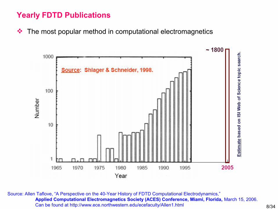
Yearly FDTD Publications

The most popular method in computational electromagnetics

Source: Allen Taflove, “A Perspective on the 40-Year History of FDTD Computational Electrodynamics,” Applied Computational Electromagnetics Society (ACES) Conference, Miami, Florida, March 15, 2006.Can be found at http://www.ece.northwestern.edu/ecefaculty/Allen1.html

9/34

Maxwell’s Equations

The basic set of equations describing the electromagnetic world Shows that light is an electromagnetic wave.

Constitutive relations

0vD

BBEtDH Jt

ρ∇ ⋅ =∇ ⋅ =

∂∇ × = −∂

∂∇ × = +∂

Gauss’s law

Gauss’s law for magnetism

Ampere’s law

Faraday’s law

,andD E B Hε µ= =

10/34

FDTD Overview – Finite Differences

Represent the derivatives in Maxwell’s curl equations by finite differences We use the second-order accurate central difference formula

( ) ( ) ( )( )2

df x f x x f x xf xdx x

+ ∆ − − ∆′= ≅∆

11/34

FDTD Overview – Cells

A three-dimensional problem space is composed of cells

12/34

FDTD Overview – The Yee Cell

The FDTD (Finite Difference Time Domain) algorithm was first established by Yee as a three dimensional solution of Maxwell's curl equations.

K. Yee, IEEE Transactions on Antennas and Propagation, May 1966.

13/34

FDTD Overview – Material grid

A three-dimensional problem space is composed of cells

14/34

FDTD Overview – Updating Equations

Three scalar equations can be obtained from one vector curl equation.

E Ht

ε ∂ = ∇ ×∂

yx zx

y x zy

y xzz

HE Ht y zE H Ht z x

H HEt x y

ε

ε

ε

∂∂ ∂= −∂ ∂ ∂

∂ ∂ ∂= −∂ ∂ ∂

∂ ∂∂ = −∂ ∂ ∂

H Et

µ ∂ = − ∇ ×∂

yx zx

y xzy

yxzz

EH Et z yH EEt x z

EEHt y x

µ

µ

µ

∂∂ ∂= −∂ ∂ ∂

∂ ∂∂= −∂ ∂ ∂

∂∂∂ = −∂ ∂ ∂

15/34

FDTD Overview – Updating Equations

Represent derivatives by finite-differences

yx zx

HE Ht y z

ε∂∂ ∂= −

∂ ∂ ∂

1

0.5 0.50.5 0.5

( , , ) ( , , )( , , )

( , , ) ( , , 1)( , , ) ( , 1, )

n nx x

x

n nn ny yz z

E i j k E i j ki j kt

H i j k H i j kH i j k H i j ky z

ε+

+ ++ +

− =∆

− −− − −∆ ∆

16/34

FDTD Overview – Updating Equations

Represent derivatives by finite-differences

yx zx

EH Et z y

µ∂∂ ∂= −

∂ ∂ ∂

0.5 0.5

0.5

( , , ) ( , , )( , , )

( , , 1) ( , , ) ( , 1, ) ( , , )

n nx x

x

n n n ny y z z

H i j k H i j ki j kt

E i j k E i j k E i j k E i j kz y

µ+ −

+

− =∆

+ − + −−∆ ∆

17/34

FDTD Overview – Updating Equations

Express the future components in terms of the past components

0.5 0.5

10.5 0.5

( , , ) ( , 1, )

( , , ) ( , , )( , , ) ( , , ) ( , , 1)

n nz z

n nx x n n

x y y

H i j k H i j kytE i j k E i j k

i j k H i j k H i j kz

ε

+ +

++ +

− − ∆∆ = − − − −

∆

0.5

0.5 0.5

( , , 1) ( , , )

( , , ) ( , , )( , , ) ( , 1, ) ( , , )

n ny y

n nx x n n

x z z

E i j k E i j kt zH i j k H i j ki j k E i j k E i j k

yµ

+

+ −

+ − ∆ ∆ = + + −− ∆

18/34

FDTD Overview – Leap-frog Algorithm

Exercise 1D

19/34

Absorbing Boundary Conditions

The three-dimensional problem space is truncated by absorbing boundaries

Most popular absorbing boundary is Perfectly Matched layers (PML)

Exercise 2D PML

20/34

Active and Passive Lumped Elements

Active and passive lumped elements can be modeled in FDTD

EH E Jt

ε σ∂∇ × = + +∂

Voltage source Current source

21/34

Active and Passive Lumped Elements

Resistor Capacitor Inductor Diode

22/34

Active and Passive Lumped Elements

A diode circuit

23/34

Transformation from Time-Domain to Frequency-Domain

Results can be obtained for frequency domain using Fourier Transform

A low-pass filter

S11

S22

Exercise 2D object

24/3424

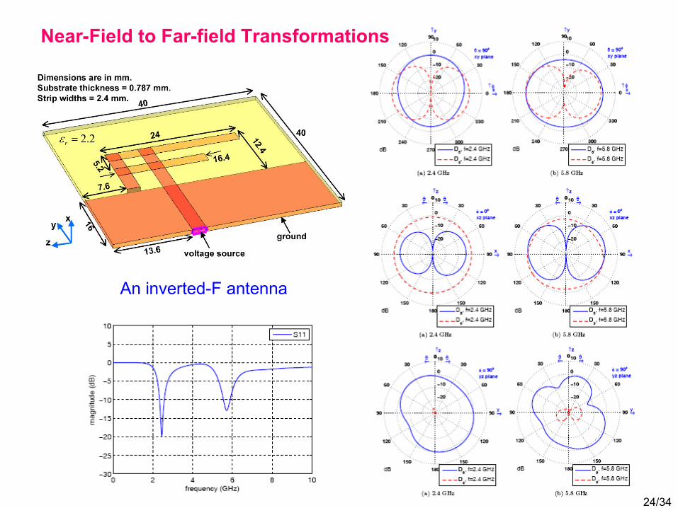
Near-Field to Far-field Transformations

An inverted-F antenna

25/34

Modeling fine geometries

It is possible to model fine structures using appropriate formulations

A wire loop antenna

26/34

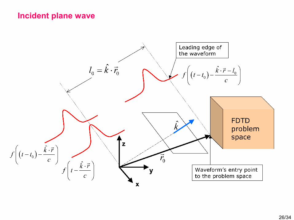
Incident plane wave

27/34

Scattering Problems

( ) ( )inc scat inc scatH H E Et

ε ∂∇ × + = +∂ 0inc incH E

tε ∂∇ × =

∂

A dielectric sphereExercise 3D PML

28/34

Scattering from a Dielectric Sphere

29/34

Earth / Ionosphere Models in Geophysics

Snapshots of FDTD-Computed Global Propagation of ELF Electromagnetic Pulse Generated by Vertical Lightning Strike off South America Coast

Source: Allen Taflove, “A Perspective on the 40-Year History of FDTD Computational Electrodynamics,” Applied Computational Electromagnetics Society (ACES) Conference, Miami, Florida, March 15, 2006.Can be found at http://www.ece.northwestern.edu/ecefaculty/Allen1.html

30/34

Wireless Personal Communications Devices

Source: Allen Taflove, “A Perspective on the 40-Year History of FDTD Computational Electrodynamics,” Applied Computational Electromagnetics Society (ACES) Conference, Miami, Florida, March 15, 2006.Can be found at http://www.ece.northwestern.edu/ecefaculty/Allen1.html

31/34

Phantom Head Validation at 1.8 GHz

Source: Allen Taflove, “A Perspective on the 40-Year History of FDTD Computational Electrodynamics,” Applied Computational Electromagnetics Society (ACES) Conference, Miami, Florida, March 15, 2006.Can be found at http://www.ece.northwestern.edu/ecefaculty/Allen1.html

32/34

Ultrawideband Microwave Detection of Early-Stage Breast Cancer

Source: Allen Taflove, “A Perspective on the 40-Year History of FDTD Computational Electrodynamics,” Applied Computational Electromagnetics Society (ACES) Conference, Miami, Florida, March 15, 2006.Can be found at http://www.ece.northwestern.edu/ecefaculty/Allen1.html

33/34

Focusing Plasmonic Lens

Source: Allen Taflove, “A Perspective on the 40-Year History of FDTD Computational Electrodynamics,” Applied Computational Electromagnetics Society (ACES) Conference, Miami, Florida, March 15, 2006.Can be found at http://www.ece.northwestern.edu/ecefaculty/Allen1.html

34/34

Thank You

Exercise 2D PEC