simulation of atmospheric rivers: dynamical modulation and...

Confidential manuscript submitted to JGR-Atmospheres

Simulation of Atmospheric Rivers: Dynamical Modulation andResolution Dependence

Erik T. Swenson1∗, Jian Lu2, and David M. Straus3

1Center for Ocean-Land-Atmosphere Studies, George Mason University, Fairfax, Virginia, USA.

2Pacific Northwest National Laboratory, Richland, Washington, USA.

3Department of Atmospheric, Oceanic, and Earth Sciences, College of Science, George Mason University, Fairfax,

Virginia, USA.

Key Points:

• More frequent long-lasting AR events found with increase in horizontal resolution

• AR event occurrence is strongly modulated by the phase and amplitude of Rossby

waves

• AR resolution sensitivity is primarily explained by changes in the local finite-amplitude

wave activity of upper-tropospheric vorticity

∗Current address, Center for Ocean-Land-Atmosphere Studies, George Mason University MSN 6C5, 4400 University

Drive, Fairfax, VA 22030

Corresponding author: Erik T. Swenson, [email protected]

–1–


Abstract

Atmospheric rivers (ARs) are examined in a set of aquaplanet simulations using the

Model for Prediction Across Scales (MPAS) dynamical core run at multiple horizontal res-

olutions, namely 240 km, 120 km and 60 km. As the resolution is increased, there is an

increase in the occurrence of long-lasting ARs. At the same time there is also an increase

in the local finite-amplitude wave activity of upper-tropospheric absolute vorticity (LWA),

a measure for Rossby wave phase and amplitude that is closely linked with wave break-

ing. Consistent with the notion that changes in ARs are driven by mid-latitude dynamics,

a strong relationship is identified between ARs and the equatorward component of LWA.

A logistic regression model is used to quantify the probability of AR occurrence based

solely on LWA and explains most of the change in AR frequency with resolution. LWA

is a diagnostic that may be easily applied to the broadly available output of CMIP6 and

other model simulations, thus enabling scientists to infer AR and wave breaking charac-

teristics. AR characteristics, in particular, require higher resolution moisture and winds at

multiple levels that are not always easily available.

1 Introduction

Atmospheric Rivers (ARs) are long and narrow regions of large moisture flux that

dominate poleward moisture transport [Zhu and Newell, 1998]. Landfalling ARs bring

intense storms and extreme precipitation during the winter [Ralph and Dettinger, 2011;

Waliser and Guan, 2017] and are closely linked to flooding over the west coasts of North

America and Europe [Ralph et al., 2006; Neiman et al., 2011; Lavers et al., 2012]. Also,

an increase in AR frequency is projected in climate change scenarios [Dettinger, 2011;

Lavers et al., 2013; Gao et al., 2016]. Thus, the ability of weather prediction models to ac-

curately forecast ARs, and the ability of climate models to realistically simulate them, are

very important concerns. Capturing these narrow and intense bands of moisture transport

may or may not require high spatial resolution [such as that used by Swain et al., 2015];

this issue is not well studied [but see Hagos et al., 2015]. Complicating the diagnosis of

ARs in many models is the need for model specific humidity and wind data at the native

model resolution, at multiple levels, and at high enough temporal resolution. Such com-

prehensive model output data sets are often not available. This is of particular concern in

assessing the affects of climate change on ARs, both because output data is limited and no

verification is possible.

–2–


Extratropical cyclones are critical for the occurrence and existence of ARs. The

local cycling of evaporation, convergence and condensation ahead of cold fronts plays

a dominant role in AR formation, while the transport of water vapor from the tropics is

typically less important [Bao et al., 2006; Sodemann and Stohl, 2013; Dacre et al., 2015].

The life cycles of extratropical cyclones are largely governed by Rossby waves identified

by planetary-scale meandering of upper-tropospheric vorticity. The phase and intensity of

Rossby waves is well-represented by the recently developed local finite-amplitude wave

activity diagnostic [Huang and Nakamura, 2016; Chen et al., 2015]. It involves integration

of a variable (such as absolute vorticity) over the area between a given contour and its

equivalent latitude, or latitude at which the area displaced equatorward is equivalent to the

area displaced poleward. Integration over these two areas yield the equatorward and pole-

ward components of local finite-amplitude wave activity, which measure the strength of

Rossby wave troughs and ridges, respectively. The equatorward component may be used

as a proxy for anticyclonic wave breaking which is closely linked with ARs [Ryoo et al.,

2013, 2015; Payne and Magnusdottir, 2014].

The purposes of this study are to

• assess the resolution dependence of ARs within a class of aquaplanet models and

• explore the association of ARs with local finite-amplitude wave activity

with the aim of better understanding the dynamical modulation of ARs and providing a

method of inferring changes in ARs when model output data is limited. The main finding

of this study is that AR occurrence and its sensitivity to model resolution can be largely

explained by local finite-amplitude wave activity.

Section 2 describes the data and methods used in this study. The composite structure

of ARs is examined in Section 3. Section 4 discusses the sensitivity to horizontal resolu-

tion, and the relationship between ARs and local finite-amplitude wave activity is exam-

ined in Section 5. A discussion and the conclusions from the study are given in Sections 6

and 7, respectively.

–3–


2 Data and methods

2.1 Aquaplanet model data

Properties of atmospheric rivers (ARs) are investigated in a set of aquaplanet sim-

ulations involving the non-hydrostatic Model for Prediction Across Scales [MPAS, Ska-

marock et al., 2012] dynamical core coupled with the Community Atmosphere Model

version 5 [CAM5, Neale et al., 2012] physics package. Results are also compared with

those from two sets of experiments run with hydrostatic and non-hydrostatic MPAS cou-

pled with the Community Atmosphere Model version 4 [CAM4, Gent et al., 2011] physics

package. The prescribed sea surface temperature distribution is symmetric about the equa-

tor and solar forcing is fixed at March equinoctial conditions, following the standard con-

trol experiment of Neale and Hoskins [2000]. Results are contrasted from simulations run

with different horizontal resolutions, namely 240 km, 120 km and 60 km. Following a

one-year spin up period, we analyze ARs from two years of 6-hourly data. Despite the

fairly short length of the simulations, ARs are quite frequent in MPAS, particularly due

to zonal symmetry and the sampling of both hemispheres. For the CAM5 (CAM4) sim-

ulations, the vertical resolution is fixed to 30 (26) levels. In order to provide a crude ob-

servational comparison, we also contrast some results with properties of wintertime (Nov.

through March) ARs over the northern Pacific and Atlantic basins identified from the ERA

Interim Reanalysis [ERAI, Dee et al., 2011].

2.2 AR detection algorithm

ARs are identified as long and narrow regions of poleward moisture flux in the sub-

tropics. The choice of criteria for AR detection follows that defined by Ralph et al. [2004]

and applied by Hagos et al. [2015], with a few important differences that are discussed

in Section 4. We first identify individual groups of contiguous grid points, or objects.

These objects are defined so that at each grid point the column-integrated precipitable wa-

ter (PW) exceeds 2 cm and the horizontal wind speed (|V |, average between two-levels

nearest to 850 hPa and 700 hPa) exceeds 10 ms−1. Additionally, in order for an object to

be considered an AR, the net direction of V must be poleward and eastward, the object

must be at least 2000 km long and less than 1000 km wide, and the mode latitude must

be poleward of 20o .

–4–


As used by Payne and Magnusdottir [2014], we also consider AR detection based on

large values of integrated moisture flux below the 700 hPa level (not shown). A typical in-

dividual AR event is similarly detected with this approach, however its areal extent tends

to be smaller, which we interpret here as the detection of the core of the AR but not the

entire feature.

2.3 Local finite-amplitude wave activity

Finite-amplitude wave activity is a diagnostic that arises out of a balance between

eddies and the zonal mean flow circulation [Nakamura and Zhu, 2010]. Huang and Naka-

mura [2016] generalize it in terms of its local longitudinal contribution. In this study, we

apply this local finite-amplitude wave activity to 300 hPa absolute vorticity. Its calcula-

tion involves integrating vorticity over the region enclosed between a given contour and

its equivalent latitude, or latitude at which the area displaced equatorward is equivalent

to the area displaced poleward. Integration over the two areas yields the equatorward and

poleward components of local finite-amplitude wave activity (LWA+ and LWA− , respec-

tively). See Appendix A for an example calculation. As previously discussed, local finite-

amplitude wave activity is a useful diagnostic for representing the phase and intensity of

Rossby waves.

2.4 Logistic regression

In this study we statistically estimate a supposed true probability (p) of AR occur-

rence with a prediction p that is conditional on a set of continuous predictors (x1, x2 and

x3). Considering that AR occurrence is binary, i.e. either an AR is present (yi = 1) or

absent (yi = 0) for the ith sample (in space and time), residuals (yi − pi) are not Gaus-

sian and follow a Bernoulli distribution. Also, we require a function for p that ensures

that 0 ≤ p ≤ 1. For these reasons, ordinary least squares is not suitable. An appropriate

approach for this is logistic regression that constructs the generalized linear model

ln( p1 − p

)= β0 + β1x1 + β2x2 + β3x3, (1)

where coefficients β0, β1, β2 and β3 are determined through maximum likelihood esti-

mation. Logistic regression assumes linearity in the relationship between the log-odds of

the probability of AR occurrence (left hand side of Eq. (1)) and the predictors x1, x2 and

x3. See Wilks [2011] for a more detailed description of logistic regression. In this study,

–5–


for predictors we use simultaneous areal-averaged values of the equatorward component of

local finite-amplitude wave activity (LWA+) upstream and downstream of AR occurrence,

and results are shown in Section 5.

2.5 Binning approach

We also estimate the probability of AR occurrence using a binning approach. Lo-

gistic regression identifies the linear relationship between the log-odds of AR occurrence

and its predictors (Eq. (1)), whereas binning is not constrained to any particular form and

thus able to represent any additional nonlinearity in the relationship (if present). Binning

is done by estimating p conditional on predictors x1, x2 and x3 for all combinations of

values falling within bins with 10 ms−1 intervals ranging from 0 − 100 ms−1 (yielding a

three-dimensional probability distribution constructed from a total of 103 bins). Results for

binning are shown in Section 5.

For estimation of p using both logistic regression and binning, as a measure of skill

we compute the Brier skill score (BSS) given by

BSS = 1 −

n∑i=1

[yi − pi]2

n∑i=1

[yi − y]2, (2)

with i corresponding to the ith sample from a total of n samples, and y giving the sample

mean AR occurrence. The numerator in Eq. (2) gives the Brier score of the prediction

while the denominator gives the Brier score of a reference forecast that simply uses the

climatological probability of AR occurrence. The BSS is less than or equal to 0 if the

prediction has no skill and 1 if the prediction is perfect.

3 Structure of Atmospheric Rivers in MPAS

Here we examine the composite structure of ARs identified in MPAS by considering

an AR-following coordinate system. For each AR that is identified, first the centroid lo-

cation (average geographic position of all grid points comprising AR) and the average tilt

angle (longitude-latitude orientation) are computed. Then, fields are horizontally shifted

and rotated in order to align AR structures, and an average is taken across all events over

the first year. Given the similarity of composites for different resolutions, results are only

shown for the 240 km simulations. Fig. 1a shows a horizontal composite centered on ARs

identified in the 240 km MPAS simulations. An AR is characterized by a relatively nar-

–6–


b) a)

Figure 1. AR composites for first year of 240 km MPAS simulation. Plotted on left (a) is precipitable wa-

ter (dark green contours, cm), 200 hPa anomalous geopotential height (black contours, m), moisture fluxes

integrated from 1000-700 hPa (red arrows, kg m−1s−1) and rainfall rate (purple, mm/day). Only moisture

flux vectors greater than 10 kg m−1s−1 are plotted. Fields are rotated according to the average tilt ( 39o )

and displayed according to the average latitudinal position ( 29o ) for all events. Heavy black line indicates

position of the abscissa for vertical cross-section shown on right (b), along which values are averaged over

20o . Plotted here is water vapor (green contours, kg m−2), horizontal wind (blue, ms−1) and moisture flux

(orange, greater than 30 kg m−1s−1) parallel to AR, along with wind (black arrows) and moisture flux (red

arrows) perpendicular to AR. Horizontal (vertical) wind and moisture flux vectors are in units of ms−1 and

kg m−1s−1 (−hPa s−1 and −hPa s−1kg m−2), respectively. In both plots, only moisture flux vectors greater

than 10 kg m−1s−1 (or −10 hPa s−1kg m−2 for vertical) are plotted. Note that a constant pressure level

approximation is used to convert model vertical coordinates to pressure for visualization in (b).

row poleward and eastward intrusion of water vapor from the tropics into the subtropics,

identified by locally high values of PW. The moisture flux associated with the AR indi-

cates transport of water vapor from the subtropics into mid-latitudes. The moisture flux

has relatively high values in the lower troposphere, with a local maximum in rainfall rate

along the leading edge of the AR. A strong mid-latitude dynamical signature is found in

terms of 200 hPa geopotential height, with a trough to the west and a ridge slightly to the

east. This is the upper-tropospheric imprint of an extratropical cyclone connected with a

cold front immediately trailing the AR [Ralph et al., 2004].

Considering the vertical structure of ARs, Fig. 1b shows a composite along a verti-

cal cross-section perpendicular to ARs. The abscissa of this plot corresponds to the heavy

line in Fig. 1a, and the component of horizontal wind (moisture flux) in the direction

along the AR of Fig. 1a is indicated by blue (orange) shading in Fig. 1b. The horizon-

–7–


tal and vertical components of the wind and moisture flux perpendicular to the AR are

indicated by black and red arrows, respectively.

The moist core is characterized by high moisture flux from the surface up to around

600 hPa (orange shading), and is associated with a jet streak in the upper troposphere

that is oriented more westerly (blue shading and black arrows). The position of maxi-

mum moisture flux along an AR is tilted slightly northwest with height, and weaker val-

ues extend northwest at lower levels. Along an AR, there is ascent of moist air (red ar-

rows) while there is descent of dry air (black arrows) off to the southeast towards the trop-

ics. Despite a large supply of tropical moisture, there appears to more moisture advected

into the extratropical side of the AR. Composites for MPAS run at 120 km and 60 km are

quite similar, however there is some narrowing of the AR core and a slight enhancement

of moisture flux at higher resolution (not shown).

4 Sensitivity to horizontal resolution

An increase in the frequency of ARs is found as horizontal resolution is increased

in the MPAS simulations. Table 1 shows the average monthly frequency of ARs, mea-

sured by the frequency of detection, and by the number of individual events. Thus an AR

event lasting for two days contributes 8 counts to the line of the table labeled “6-hourly”,

but contributes only 1 count to the line labeled “event”. In addition, we report the aver-

age event duration given in days. The AR frequency is higher in the 120 km simulations

than that in the 240 km simulations due to the fact that AR events persist longer, whereas

an additional modest increase in AR frequency in the 60 km simulations is not related to

duration but simply to increased occurrence.

Table 1. Average monthly frequency of ARs counted in terms of detection at each 6-hourly interval (first

row) and in terms of individual events with variable duration (second row). Also, average event duration

is given in days (third row). Results are shown for MPAS simulations run at 240 km, 120 km and 60 km

horizontal resolution (columns as labeled).

ARs/month 240 km 120 km 60 km

6-hourly 706 817 840

event 110 108 114

duration 1.6 1.9 1.8

–8–


The significant increase in AR frequency when increasing the horizontal resolution

from 240 km to 120 km is also found in MPAS simulations run with CAM4 hydrostatic

and non-hydrostatic dynamical cores (Table 2). Here our frequency counts differ greatly

from those of Hagos et al. [2015, see their Fig. 2] who find an order of magnitude less

overall AR occurrence and a decrease with increasing resolution. This discrepancy is pri-

marily due to our lack of requiring 75-80% of the total PW to be concentrated below the

800 hPa level. In all the MPAS simulations, we find that ARs have a substantial fraction

of water vapor above the 800 hPa level, and applying such a vertical constraint yields

an order of magnitude reduction in AR frequency to values consistent with Hagos et al.

[2015] (not shown).

Table 2. Average monthly frequency of ARs counted in terms of detection at each 6-hourly interval using

CAM5 non-hydrostatic (first row), CAM4 non-hydrostatic (second row) and CAM4 hydrostatic (third row)

dynamical cores for MPAS simulations run at 240 km, 120 km and 60 km horizontal resolution (columns as

labeled). Also given are differences in AR frequency between 120 km simulations and 240 km simulations

(column labeled ∆120 km) and additional differences between 60km simulations and 120 km simulations

(column labeled ∆60 km).

ARs/month 240 km 120 km 60 km ∆120 km ∆60 km

CAM5 non-hyd 706 817 840 +111 +23

CAM4 non-hyd 677 782 787 +105 +5

CAM4 hyd 747 844 815 +97 −29

We also find a clear narrowing of ARs when increasing horizontal resolution. This

is reflected in a shift in the frequency distribution of AR width (Fig. 2). The mean width

of AR events for the 240 km, 120 km and 60 km simulations is 655 km, 588 km and 534

km, respectively. As resolution is increased, the most notable difference is a substantial

increase in narrow AR events (widths < 400 km) which is largely balanced by a broader

decrease in wide AR events (widths > 600 km). Comparison to the AR width distribution

estimated from ERAI (normalized by number of events from MPAS simulations) suggests

that the general shift in the distribution of AR width is not an improvement. The propor-

tion of wide AR events is underestimated, and this is worsened as resolution is increased

and the proportion of narrower events becomes overestimated. Nevertheless, a significant

fraction of narrow AR events that occur in ERAI are simulated at 120 km and 60 km yet

–9–


200 400 600 800 1000

020

040

060

080

0

width (km)200 400 600 800 1000

020

040

060

080

0

200 400 600 800 1000

020

040

060

080

0fre

quen

cy

MPAS 240 kmMPAS 120 km

all events

200 400 600 800 1000

020

040

060

080

0

width (km)200 400 600 800 1000

020

040

060

080

0

200 400 600 800 1000

020

040

060

080

0fre

quen

cy


all events

Figure 2. Histograms of AR width for MPAS simulations plotted for width intervals of 20 km. On left,

frequency of AR width plotted for 240 km simulations and 120 km simulations for which blue (red) indicates

higher frequency in 240 km (120 km) simulations. On right, frequency of AR width plotted for 240 km simu-

lations and 60 km simulations for which blue (red) indicates higher frequency in 240 km (60 km) simulations.

AR width frequency is counted in terms of detection at each 6-hourly interval. The distribution of AR width

estimated from ERAI (normalized to have the same total frequency of occurrence averaged over all MPAS

simulations) is shown by a black line.

unresolved at 240 km. Note also that interpolation to a common 240 km grid prior to AR

detection results in a reduction in frequency; thus we do not apply prior interpolation in

this study.

We further examine frequency distributions of various AR characteristics in or-

der to better understand changes in event duration. We focus on the differences between

ARs in the MPAS simulations run at 240 km and those in the simulations run at 120 km,

which captures the most significant change in frequency with resolution (60 km results

are similar to 120 km results). The increase in event duration is evident in the fact that

long-lasting events are consistently more frequent in the higher resolution simulations,

and the distribution of event duration has a thicker and longer tail with higher values (Fig.

3). This result stands out in CAM4 hydrostatic and non-hydrostatic simulations as well

(not shown). We also find an increase in more zonally-oriented ARs (indicated by tilt an-

gles < 40o , Fig. 3). By partitioning events as either short-lived (≤ 3 days) or long-lived

(> 3 days), comparison between conditional frequency distributions of AR tilt reveals that

the more frequent long-lasting events do tend to be more zonally-oriented. AR events in

ERAI tend to have a broader tilt distribution, and there tends to be relatively fewer long-

–10–


0 5 10 15 20

02

46

8duration (days)

0 5 10 15 20

02

46

8

0 5 10 15 20

02

46

8lo

g fre

quen

cy3


short long

0 20 40 60 80

020

040

060

080

010

0012

00

tilt (degrees)0 20 40 60 80

020

040

060

080

010

0012

00

0 20 40 60 80

020

040

060

080

010

0012

00fre

quen

cy


all events

0 20 40 60 80

010

020

030

040

050

060

070

0


010

020

030

040

050

060

070

0

0 20 40 60 80

010

020

030

040

050

060

070

0fre

quen

cy


short−lived

0 20 40 60 80

010

020

030

040

050

060

070

0


010

020

030

040

050

060

070

0

0 20 40 60 80

010

020

030

040

050

060

070

0fre

quen

cy


long−lived

Figure 3. Histograms of AR event duration (in terms of log frequency, top left) and AR tilt (top right). Blue

(red) indicates higher frequency in MPAS simulations run at 240 km (120 km) resolution. AR tilt frequency

is represented in terms of 6-hourly detection and is also separated according to short-lived (≤ 3 days, lower

left) and long-lived (> 3 days, lower right) events. The corresponding distributions estimated from ERAI

(normalized to have the same total frequency of occurrence averaged over all MPAS simulations) are shown

by black lines.

lasting events. This could be due to a number of factors, but we hypothesize that AR du-

ration and tilt is largely constrained by the presence of stationary waves and the interrup-

tion of land and orography.

5 Relationship between ARs and wave activity

Changes in water vapor and/or the jet stream could theoretically provide insight into

changes in AR frequency [Hagos et al., 2015]. However there are only subtle differences

in climatological mean zonal wind among the three non-hydrostatic CAM5 simulations

examined here [Zhao et al., 2016, see their Fig. 6], and very little variation in climatolog-

ical mean water vapor as well (not shown). What does vary with resolution a great deal

is the climatological time and zonal mean local finite-amplitude wave activity of 300 hPa

absolute vorticity. There is a clear increase in both the equatorward and poleward compo-

–11–


Figure 4. Climatological time and zonal mean finite-amplitude wave activity of 300 hPa absolute vorticity

(ms−1) plotted as a function of latitude (abscissa) for the MPAS simulations run at 240 km (black), 120 km

(blue) and 60 km (red). Plotted separately is the equatorward component (zonal mean LWA+, solid lines) and

the poleward component (zonal mean LWA− , dashed lines).

nents of this wave activity, denoted by LWA+ and LWA− , respectively, as shown in Fig.

4.

The association of AR events with LWA+ can be seen by considering a randomly-

chosen synoptic time sample from the MPAS simulations (Fig. 5). In this figure, equator-

ward wave activity (LWA+) is given in orange-red shading, the precipitable water in green

shading, and 300 hPa absolute vorticity in black contours. Individual ARs are denoted

by purple contours. The strength of Rossby wave troughs is well represented by local

maxima in LWA+, which modulate the longitudinal position of ARs. Note that the spa-

tial variation of 300 hPa absolute vorticity is sensitive to horizontal resolution, and tight

gradients associated with filaments of relatively high vorticity are present in 120 km and

60 km simulations but entirely unresolved in the 240 km simulation. LWA+ provides a de-

gree of spatial filtering and tends to isolate planetary-scale zonal asymmetry [Huang and

Nakamura, 2016].

The relationship between ARs and LWA+ is evident from fields composited rela-

tive to the centroid longitude of all AR events identified in the MPAS simulations run at

240 km (Fig. 6). ARs tend to be phase-locked with a trough-ridge-trough pattern associ-

ated with local extrema in mid-latitude LWA+ projecting onto wavenumber 6-7. Based on

–12–


Figure 5. Sample of LWA+ (orange-red shading, ms−1), 300 hPa absolute vorticity (contours, intervals of

5 × 10−5s−1), precipitable water (PW, cm) and AR events (thick purple contours) for MPAS simulations run

at (a) 240 km, (b) 120 km and (c) 60 km. Probability of AR occurrence predicted by logistic regression with

LWA+ for 20o longitude sections printed in purple.

this local pattern in simultaneous LWA+, we select predictors for statistically estimating

the probability of AR occurrence p from LWA+ alone. We represent coincident LWA+ by

three areal averages over 25o longitude-width neighboring boxes across the 30 − 60o mid-

latitude band, immediately upstream (x1) and immediately downstream (x2 and x3), as

depicted by black boxes in Fig. 6. These LWA+ predictors are related to AR occurrence

within a given 20o longitude segment and time (according to centroid longitude of AR,

depicted by blue box in Fig. 6). Data is pooled together from the MPAS simulations run

at all three horizontal resolutions. This provides a total sample size of n = 315,360. Note

that statistical relationships are highly significant, and if relationships are constructed from

one year of data (instead of two years), there is very little reduction in skill applying them

to the other year (not shown).

–13–


y

x3

| − 25o − |

x1 x2

| − 20o − |

Figure 6. Longitude-centered AR composite for 240 km MPAS simulation. Plotted is LWA+ (orange-red

shading, ms−1), 300 hPa absolute vorticity (contours, intervals of 5 × 10−5s−1), and precipitable water (PW,

cm, thick green contour indicates 2 cm). LWA+ averaging regions used to construct predictors for logistic

regression are shown by black rectangles, and longitudinal region for predicting probability of AR occurrence

is shown by a blue rectangle.

First, we construct a logistic regression model based on the LWA+ predictors (see

Section 2 for details). This reveals a robust linear relationship between the log-odds of

AR occurrence and LWA+ given by

ln( p1 − p

)= −1.8 + 0.03x1 − 0.06x2 + 0.02x3, (3)

which provides a skillful estimate of the probability of AR occurrence at any given loca-

tion and time with a BSS of 0.336. A very similar relationship explains AR occurrence

with a BSS of 0.347 and 0.330 in the CAM4 hydrostatic and non-hydrostatic MPAS sim-

ulations, respectively. Consistent with Figs. 5 and 6, regression coefficients indicate that

an AR event is more probable (large p) when mid-latitude LWA+ is high immediately up-

stream, low immediately downstream, and high further downstream. On the other hand, an

AR event is quite unlikely (small p) when the opposite is true, which tends to occur 25o

out of phase of regions of high probability of occurrence. In Fig. 5, the value of p esti-

mated from logistic regression is printed for each 20o longitude segment, and AR events

tend to lie in regions with relatively higher probabilities (typically 0.35 < p < 0.55) while

neighboring regions tend to have probabilities near zero.

–14–


20 40 60 80

0.0

0.1

0.2

0.3

0.4

0.5

0.6

Upstream LWA+ (x1)

p

CAM5 non−hyd

CAM4 non−hyd

CAM4 hyd

Figure 7. Probability of AR occurrence (p) as a function of upstream LWA+ (x1, ms−1) estimated from

logistic regression (dashed lines) and from binning (solid lines). Results are shown for MPAS simulations run

with CAM5 non-hydrostatic (black), CAM4 non-hydrostatic (blue) and CAM4 hydrostatic (red) dynamical

cores.

In terms of the log-odds of AR occurrence, Eq. (3) quantifies a robust linear rela-

tionship with LWA+, however there does appear to be a degree of nonlinearity that is not

represented by logistic regression. In order to address this, we also estimate p through a

binning approach, as discussed in Section 2. First, consider p as a function of only up-

stream LWA+, or x1 alone (Fig. 7). For binning (solid lines) compared with logistic re-

gression (dashed lines), p is relatively more sensitive to low values of LWA+ (for values

less than about 40 ms−1) and less sensitive to high values of LWA+ (for values greater

than about 60 ms−1). There is some indication of a threshold at which AR occurrence

no longer increases with LWA+. This behavior is found in both CAM5 and CAM4 non-

hydrostatic simulations. For these simulations, modestly more variation in AR occurrence

is explained by estimating p from binning according to the values of all three LWA+ pre-

dictors in comparison to logistic regression (not shown). However there is much less of a

distinction between approaches in the CAM4 hydrostatic simulations where the relation-

ship is more linear.

While a significant amount of local variation in AR occurrence is explained by

LWA+, a central question in this study is to what degree does LWA+ explain the sensi-

–15–


tivity of climatological AR frequency to horizontal resolution? This is addressed by av-

eraging p over each simulation and normalizing by the number of months, resulting in

the climatological AR frequency estimated from LWA+ through logistic regression (Ta-

ble 3) and through binning (Table 4). We find that about 50-70% of the increase in AR

frequency in the 120 km simulations (relative to the 240 km simulations) is explained by

changes in LWA+. In the CAM5 and CAM4 non-hydrostatic simulations, roughly 20% of

this increase is explained by nonlinearity in the relationship with LWA+. This quantifies a

strong dynamical modulation in the sensitivity of AR frequency to horizontal resolution.

On the other hand, further changes in AR frequency in the 60 km simulations are weaker

and inconsistent, and generally not explained by changes in LWA+.

Table 3. Same as Table 2, but that estimated by logistic regression model using LWA+.


CAM5 non-hyd 743 804 799 +64 −5

CAM4 non-hyd 712 750 769 +38 +19

CAM4 hyd 752 815 828 +63 +13

Table 4. Same as Table 3, but that estimated by binning based on values of LWA+ predictors with bin

widths of 10 ms−1.


CAM5 non-hyd 716 794 787 +78 −7

CAM4 non-hyd 685 748 766 +63 +18

CAM4 hyd 733 782 808 +49 +26

6 Discussion

In the MPAS aquaplanet simulations, there is a clear modulation of the spatiotempo-

ral variation in probability of AR occurrence by the phase and amplitude of mid-latitude

Rossby waves, as measured by the equatorward component of local finite-amplitude wave

activity of 300 hPa absolute vorticity (LWA+). LWA+ largely determines the location and

timing of AR events. It also explains most of the increase in AR frequency in the 120

–16–


km simulations (compared with 240 km simulations) that is due to longer lifetimes of AR

events. Long-lasting AR events tend to be more zonally-oriented, and further investigation

reveals that they tend to coincide with long-lasting regions of high LWA+ that are also

more frequent in the 120 km simulations (not shown). This is consistent with a stronger

linkage between anticyclonic wave breaking (reflected in LWA+) and long-lasting ARs

(relative to short-lived AR events).

The three-dimensional structure of ARs is simulated fairly well in the MPAS simu-

lations run at all horizontal resolutions. Composites suggest that there may be more mois-

ture advection into an AR along its extratropical boundary compared with that along its

tropical boundary. Nevertheless, the role of moisture flux cannot be quantified here with-

out some kind of moisture budget calculation. In this regard, Dacre et al. [2015] com-

pute a moisture budget but relative to extratropical cyclones as a whole. Lu et al. [2017]

quantify the hydrological cycle of ARs through the application of finite-amplitude wave

activity to column-integrated water vapor, however a relevant distinction is not made in

terms of the location of moisture flux into ARs. This motivates further work towards un-

derstanding the role of moisture advection for ARs.

As horizontal resolution is increased, we find a slight enhancement in moisture flux

along ARs, and more notably a narrowing of ARs. There is a general tendency for ARs

to narrow throughout their lifetimes (not shown). In terms of the wave activity of water

vapor itself (as investigated by Lu et al. [2017]), we find a reduction in its dissipation as

resolution is increased (not shown). This may explain part of the reason why there are

more long-lasting ARs in the 120 km simulations compared with the 240 km simulations.

Consistent with a reduction in mid-latitude LWA+, it is likely that the 240 km simulations

are too numerically diffusive. Consequently, this resolution may be inadequate for resolv-

ing very tight moisture gradients along ARs consistent with that observed [e.g., see Ralph

et al., 2004]. Nevertheless, the further narrowing of ARs in the 60 km simulations is not

realistic in terms of the shape of AR width distribution (compared with that from ERAI).

The relationship between LWA+ and ARs along with resolution sensitivity of AR

characteristics (contrasting 120 km simulations with 240 km simulations) are echoed in

the hydrostatic and non-hydrostatic CAM4 MPAS simulations. All simulations agree in

an increase in AR frequency with resolution due to more frequent long-lasting AR events,

which is largely explained by changes in LWA+. Further work should be done towards in-

–17–


vestigating the relationship between LWA+ and ARs in the presence of stationary waves

forced by ocean-land asymmetry, and its relevance at intra-seasonal to inter-annual time-

scales. Along these lines, we also construct a similar logistic regression model for win-

tertime AR occurrence over the Pacific and Atlantic basins estimated in ERAI. In agree-

ment with the MPAS results, LWA+ explains a comparable amount of the variation in AR

occurrence with a BSS of roughly 0.27. However, preliminary results indicate that this

LWA+ logistic regression model explains only a small fraction of the inter-annual variabil-

ity in AR occurrence.

Considering that local finite-amplitude wave activity explains much of the resolu-

tion sensitivity of AR occurrence, it could theoretically provide insight into the response

of ARs to global warming and/or model-to-model differences. The wave activity diagnos-

tic may be applied to various readily-available variables such as geopotential height [Chen

et al., 2015]. Given the direct relationship to vorticity, we hypothesize that wave activity

of mid-tropospheric geopotential height explains a comparable amount of variation in AR

occurrence. Application of this diagnostic is encouraged for CMIP6 and other model sim-

ulations in order to better understand and/or infer changes in ARs.

7 Conclusions

The primary finding in this study is the sensitivity of atmospheric river (AR) char-

acteristics to horizontal model resolution, and how this sensitivity is largely explained by

changes in mid-latitude Rossby waves. In the MPAS simulations, we find a significant in-

crease in AR frequency as horizontal resolution is increased from 240 km to 120 km. This

is due to the fact that ARs tend to have longer lifetimes in the 120 km simulations. We

also find a progressive narrowing of ARs when increasing resolution to 120 km and 60

km. These changes are quite robust and reproducible in the CAM4 non-hydrostatic and

hydrostatic MPAS simulations.

The resolution sensitivity of ARs in the CAM5 non-hydrostatic MPAS simulations

cannot be simply explained by a moistening or shift in the upper-tropospheric jet be-

cause differences in climatological mean water vapor and zonal wind are negligible. There

is however an increase in the equatorward component of the climatological local finite-

amplitude wave activity of 300 hPa absolute vorticity (LWA+). LWA+ is a good mea-

sure for the strength of Rossby wave troughs which strongly modulates the probability

–18–


of AR occurrence. We find a correspondence between longer lifetimes of AR events and

more persistent regions of large LWA+. Long-lasting AR events tend to be more zonally-

oriented and more strongly linked with downstream anticyclonic wave breaking.

We construct two statistical models relating instantaneous mid-latitude LWA+ with

AR occurrence and find that a significant amount of the variation in AR occurrence is ex-

plained by LWA+ alone. Furthermore, LWA+ explains 50-70% of the increase in AR fre-

quency in the 120 km simulations (relative to the 240 km simulations), and these results

are also reproducible in the CAM4 non-hydrostatic and hydrostatic MPAS simulations.

Weaker changes in AR characteristics in the 60 km simulations (relative to the 120 km

simulations) are not consistently reproduced nor explained by LWA+.

A: Calculation of local finite-amplitude wave activity

Here we show an example calculation of local finite-amplitude wave activity for the

same synoptic time sample of the 240 km MPAS simulation shown in Fig. 5a. The calcu-

lation is illustrated in Fig. A1 in application to 300 hPa absolute vorticity (gray contours

in Fig. A1a), and follows the conceptual example of Huang and Nakamura [2016, see

their Fig. 1]. Considering the 11 × 10−5s−1 contour (thick black contour), the equivalent

latitude (thick gray line) is defined as the latitude at which the area displaced equatorward

of the equivalent latitude by this contour (region covered by orange-red shading) is equiv-

alent to the area displaced poleward (region covered by blue shading). This calculation

involves the meridional displacement at all longitudes (not limited to smaller domain plot-

ted) and yields an equivalent latitude of 42.6o N . Along this latitude (thick gray line in

Fig. A1a), local finite-amplitude wave activity is computed in terms of its equatorward

and poleward components (LWA+ and LWA− , respectively, Fig. A1b). At a given longi-

tude, the value of LWA+ is equal to the integral of absolute vorticity over the latitudinal

range displaced equatorward (orange-red shading), and the value of LWA− is equal to in-

tegral of absolute vorticity over the latitudinal range displaced poleward (blue shading)

multiplied by −1. This is repeated for values spanning the range of the absolute vorticity

contours (with associated equivalent latitudes) to yield two-dimensional fields of LWA+

and LWA− shown in Fig. A1c (orange-red and blue shading, respectively).

–19–


Acknowledgments

This work was supported by the Department of Energy under grant DE-SC0012599. JL

was supported by the U.S. Department of Energy Office of Science Biological and Envi-

ronmental Research (BER) as part of the Regional and Global Climate Modeling program.

DMS was also supported by NSF grant AGS-1338427, NOAA grant NA14OAR4310160,

and NASA grant NNX14AM19G. The data has been archived on the HPSS of the Na-

tional Energy Research Scientific Computing Center (NERSC), and can be accessed upon

request.

References

Bao, J.-W., Michelson, S. A., Neiman, P. J., Ralph, F. M. and Wilczak J. M. (2006), In-

terpretation of enhanced integrated water vapor bands associated with extratropical cy-

clones: Their formation and connection to tropical moisture, Mon. Wea. Rev. 134, 1063–

1080, doi:10.1175/MWR3123.1.

Chen, G., Lu, J., Burrows, D. A., and Leung, L. R. (2015), Local finite-amplitude wave

activity as an objective diagnostic of midlatitude extreme weather, Geophys. Res. Lett.

42, 10,952–10,960, doi:10.1002/2015GL066959.

Dacre, H. F., Clark, P. A., Martinez-Alvarado, O., Stringer, M. A., and Lavers, D. A.

(2015), How do atmospheric rivers form? Bull. Amer. Meteor. Soc. 96, 1243–1255,

doi:10.1175/BAMS-D-14-00031.1.

Dee, D. P., Uppala, S. M., Simmons, A. J., Berrisford, P., Poli, P., Kobayashi, S., Andrae,

U., Balmaseda, M. A., Balsamo, G., Bauer, P., Bechtold, P., Beljaars, A. C. M., van

de Berg, L., Bidlot, J., Bormann, N., Delsol, C., Dragani, R., Fuentes, M., Geer, A.

J., Haimberger, L., Healy, S. B., Hersbach, H., Hólm, E. V., Isaksen, L., Kållberg, P.,

Köhler, M., Matricardi, M., McNally, A. P., Monge-Sanz, B. M., Morcrette, J.-J., Park,

B.-K., Peubey, C., de Rosnay, P., Tavolato, C., Thépaut, J.-N., and Vitart, F. (2011), The

ERA-Interim reanalysis: configuration and performance of the data assimilation system,

Quart. J. Roy. Meteor. Soc. 137, 553–597, doi:10.1002/qj.828.

Dettinger, M. D. (2011), Climate change, atmospheric rivers and floods in California - A

multimodel analysis of storm frequency and magnitude changes, J. Amer. Water Resour.

Assoc. 47, 514–523, doi:10.1111/j.1752-1688.2011.00546.x.

Gao, Y., Lu, J., and Leung, L. R. (2016), Uncertainties in projecting future changes in

atmospheric rivers and their impacts on heavy precipitation over Europe, J. Climate 29,

–20–


6711–6726, doi:10.1175/JCLI-D-16-0088.1.

Gent, P. R., Donner, L. J., Holland, M. M., Hunke, E. C., Jayne, S. R., Lawrence, D. M.,

Neale, R. B., Rasch, P. J., Vertenstein, M., Worley, P. H., Yang, Z.-L., and Zhang, M.

(2011), The Community Climate System Model version 4, J. Climate 24, 4973–4991,

doi:10.1175/2011JCLI4083.1.

Hagos, S., Leung, L. R., Yang, Q., Zhao, C., and Lu, J. (2015), Resolution and dynamical

core dependence of atmospheric river frequency in global model simulations, J. Climate

28, 2764–2776, doi:10.1175/JCLI-D-14-00567.1.

Huang, C. S. Y., and Nakamura, N. (2016), Local finite-amplitude wave activity as a diag-

nostic of anomalous weather events, J. Atmos. Sci. 73, 211–229, doi:10.1175/JAS-D-15-

0194.1.

Lavers, D. A., Villarini, G., Allan, R. P., Wood, E. F., and Wade, A. J. (2012), The de-

tection of atmospheric rivers in atmospheric reanalyses and their links to British winter

floods and the large-scale climatic circulation, J. Geophys. Res. Atmos. 117, D20106,

doi:10.1029/2012JD018027.

Lavers, D. A., Allan, R. P., Villarini, G., Lloyd-Hughes, B., Brayshaw, D. J., and Wade,

A. J. (2013), Future changes in atmospheric rivers and their implications for winter

flooding in Britain, Environ. Res. Lett. 8, 034010, doi:10.1088/1748-9326/8/3/034010.

Lu, J., Sakaguchi, K., Yang, Q., Leung, L. R., Chen, G., Zhao, C., Swenson, E. and Hou,

Z. J. (2017), Examining the hydrological variations in an aquaplanet world using wave

activity transformation, J. Climate 30, 2559–2576, doi:10.1175/JCLI-D-16-0561.1.

Nakamura, N., and Zhu, D. (2010), Finite-amplitude wave activity and diffusive flux

of potential vorticity in eddy-mean flow interaction, J. Atmos. Sci. 67, 2701–2716,

doi:10.1175/2010JAS3432.1.

Neale, R. B., and Hoskins, B. J. (2000), A standard test for AGCMs including

their physical parameterizations. I: The proposal, Atmos. Sci. Lett. 1, 101–107,

doi:10.1006/asle.2000.0022.

Neale, R. B., Chen, C.-C., Gettelman, A., Lauritzen, P. H., Park, S., Williamson, D. L.,

Conley, A. J., Garcia, R., Kinnison, D., Lamarque, J.-F., Marsh, D., Mills, M., Smith,

A. K., Tilmes, S., Vitt, F., Morrison, H., Cameron-Smith, P., Collins, W. D., Iacono, M.

J., Easter, R. C., Ghan, S. J., Liu, X., Rasch, P. J., and Taylor, M. A. (2012). Descrip-

tion of the NCAR Community Atmosphere Model (CAM 5.0), Tech. rep., NCAR/TN-

486+STR, NCAR Tech. Note, 244pp.

–21–


Neiman, P. J., Schick, L. J., Ralph, F. M, Hughes, M., and Wick, G. A. (2011), Flood-

ing in western Washington: The connection to atmospheric rivers, J. Hydrometeor. 12,

1337–1358, doi:10.1175/2011JHM1358.1.

Payne, A. E., and Magnusdottir, G. (2014), Dynamics of landfalling atmospheric rivers

over the North Pacific in 30 years of MERRA reanalysis, J. Climate 27, 7133–7150,

doi:10.1175/JCLI-D-14-00034.1.

Ralph, F. M, Neiman, P. J., and Wick, G. A. (2004), Satellite and CALJET air-

craft observations of atmospheric rivers over the eastern North Pacific Ocean dur-

ing the winter of 1997/98, Mon. Wea. Rev. 132, 1721–1745, doi:10.1175/1520-

0493(2004)132<1721:SACAOO>2.0.CO;2.

Ralph, F. M, Neiman, P. J., Wick, G. A., Gutman, S. I., Dettinger, M. D., Cayan, D. R.,

and White, A. B. (2006), Flooding on California’s Russian River: Role of atmospheric

rivers, Geophys. Res. Lett. 33, L13801, doi:10.1029/2006GL026689.

Ralph, F. M, and Dettinger, M. D. (2011), Storms, floods, and the science of atmospheric

rivers, EOS 92, 265–266, doi:10.1029/2011EO320001.

Ryoo, J.-M., Kaspi, Y., Waugh, D. W., Kiladis, G. N., Waliser, D. E., Fetzer, E. J., and

Kim, J. (2013), Impact of Rossby wave breaking on U.S. west coast winter precipitation

during ENSO events, J. Climate 26, 6360–6382, doi:10.1175/JCLI-D-12-00297.1.

Ryoo, J.-M., Waliser, D. E., Waugh, D. W., Wong, S., Fetzer, E. J., and Fung, I. (2015),

Classification of atmospheric river events on the U.S. west coast using a trajectory

model, J. Geophys. Res. Atmos. 120, 3007–3028, doi:10.1002/2014JD022023.

Skamarock, W. C., Klemp, J. B., Duda, M. G., Fowler, L., Park, S.-H., and Ringler, T.

D. (2012), A multiscale nonhydrostatic atmospheric model using centroidal Voronoi

tesselations and C-grid staggering, Mon. Wea. Rev. 240, 3090–3105, doi:10.1175/MWR-

D-11-00215.1.

Sodemann, H., and Stohl, A. (2013), Moisture origin and meridional transport in atmo-

spheric rivers and their association with multiple cyclones, Mon. Wea. Rev. 141, 2850–

2868, doi:10.1175/MWR-D-12-00256.1.

Swain, D. L., Lebassi-Habtezion, B., and Diffenbaugh, N. S. (2015), Evaluation of nonhy-

drostatic simulations of Northeast Pacific atmospheric rivers and comparison to in situ

observations, Mon. Wea. Rev. 143, 3556–3569, doi:10.1175/MWR-D-15-0079.1.

Waliser, D. E., and Guan, B. (2017), Extreme winds and precipitation during landfall of

atmospheric rivers, Nat. Geosci. 10, 179–184, doi:10.1038/ngeo2894.

–22–


Wilks, D. S. (2011), Statistical methods in the atmospheric sciences. Academic Press, 3,

519–562.

Zhao, C., Leung, L. R., Park, S.-H., Hagos, S., Lu, J., Sakaguchi, K., Yoon, J., Har-

rop, B. E., Skamarock, W., and Duda, M. G. (2016), Exploring the impacts of

physics and resolution on aqua-planet simulations from a nonhydrostatic global

variable-resolution modeling framework, J. Adv. Model. Earth Syst. 8, 1751–1768,

doi:10.1002/2016MS000727.

Zhu, Y., and Newell, R. E. (1998), A proposed algorithm for moisture fluxes

from atmospheric rivers, Mon. Wea. Rev. 126, 725–735, doi:10.1175/1520-

0493(1998)126,0725:APAFMF.2.0.CO;2.

–23–


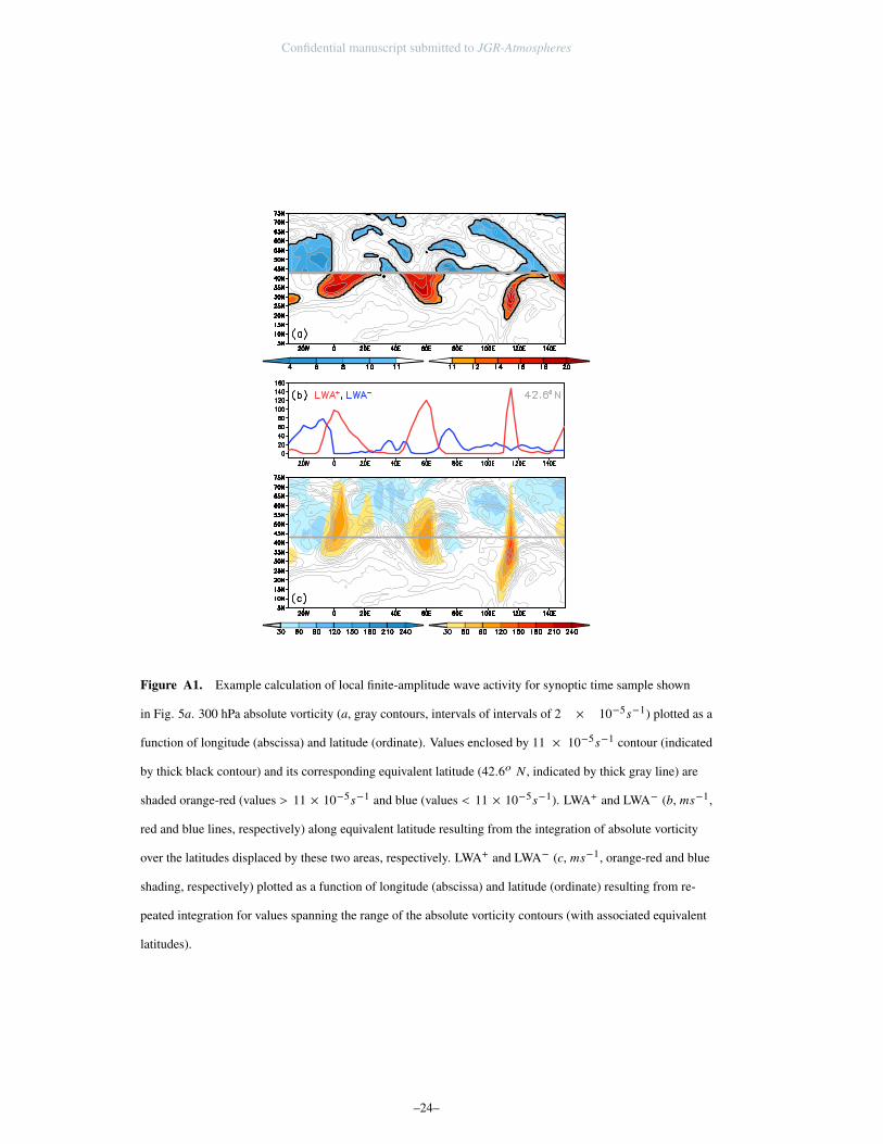
Figure A1. Example calculation of local finite-amplitude wave activity for synoptic time sample shown

in Fig. 5a. 300 hPa absolute vorticity (a, gray contours, intervals of intervals of 2 × 10−5s−1) plotted as a

function of longitude (abscissa) and latitude (ordinate). Values enclosed by 11 × 10−5s−1 contour (indicated

by thick black contour) and its corresponding equivalent latitude (42.6o N , indicated by thick gray line) are

shaded orange-red (values > 11 × 10−5s−1 and blue (values < 11 × 10−5s−1). LWA+ and LWA− (b, ms−1,

red and blue lines, respectively) along equivalent latitude resulting from the integration of absolute vorticity

over the latitudes displaced by these two areas, respectively. LWA+ and LWA− (c, ms−1, orange-red and blue

shading, respectively) plotted as a function of longitude (abscissa) and latitude (ordinate) resulting from re-

peated integration for values spanning the range of the absolute vorticity contours (with associated equivalent

latitudes).

–24–

simulation of atmospheric rivers: dynamical modulation and...

Documents