simulation of aircraft manoeuvres based on computational...

Simulation of Aircraft Manoeuvres Based On

Computational Fluid Dynamics

M. Ghoreyshi∗, D. Vallespin †, A.Da Ronch ‡ and K. J. Badcock§

Department of Engineering, University of Liverpool, Liverpool, UK, L69 3GH

J.Vos ¶

CFS Engineering, Lausaunne, Switzerland

S.Hitzel‖

EADS Military Air Systems, Munich, Germany

The use of computational fluid dynamics to generate and test aerodynamic data tablesfor flight dynamics analysis is described in this paper. The test case used is the Ranger2000 fighter trainer for which flight test data is available. The generation of the tables isdone using sampling and reconstruction to allow a large number of table entries to be gen-erated at low computational cost. The testing of the tables is done by replaying, through atime accurate CFD calculation which features the moving control surfaces, manoeuvres andcomparing the forces and moments against the tabular values. The manoeuvres are gener-ated using a time optimal prediction code with the feasible solutions based on the tabularaerodynamics. The generated maneouvres are evaluated against flight data to show thatthey are qualitatively representative. Then the time accurate and tabular aerodynamicsare compared, and as expected are in close agreement.

I. Introduction

The aerodynamic forces acting on aircraft need to be estimated for the analysis of the vehicle’s motion.The formulation of these forces date back to the early 1900s, when G.H. Bryan and W.E. Williams1 introducedthe first stability-derivatives aerodynamic model, which is still found reliable for conventional aircraft inaerodynamically benign regions of the flight envelope. To meet the demands of accurately modeling theaerodynamics of manoeuvring aircraft, some improved methods are required for representing the nonlinearand unsteady flows around the aircraft.2–4 The source of nonlinearity and unsteadiness is mainly due toshock waves, separation and vortices at high angles of attack.5 The prediction of the flows over aircraft withhigh angle of attack and large amplitude manoeuvres is complicated by the fact that aerodynamic forcesand moments of aircraft responding to sudden changes of flow not only depends on the instantaneous valuesbut also the time history of the motion.6 There have only been a limited number of attempts to include thenonlinearity and unsteadiness. Examples include the work of Tobak and his colleagues7 for the non-linearindicial response methods, and Goman and Khrabov for the state-space model.8 The basic parameters ofboth methods are often identified based on the measured flight test data,9 but for a comprehensive model,a large number of training manoeuvres are needed that makes such a model very expensive.

Traditionally, aerodynamic data are obtained from wind tunnel testing or flight test data. The windtunnel experiments can be expensive and suffer from scaling issues, along with difficulty in representing somedynamic motions.10,11 The flight test data are also very expensive and available late in the development.Today, CFD tools are becoming credible for simulating the physics of the aerodynamic flow. In principle,

∗Research Associate, AIAA member†Ph.D Student, AIAA member‡Ph.D Student, AIAA member§Professor, AIAA senior member, Corresponding author, E-mail: [email protected]¶Director of CFS Engineering‖Technical Head and Doctor of Aerodynamics

1 of 21

American Institute of Aeronautics and Astronautics

CFD can produce the aerodynamic inputs for the formulation of aircraft loads, also, simulate directly theaerodynamic responses of a manoeuvring aircraft by coupling the time-dependent Reynolds-Averaged Navier-Stokes (RANS) equations and the dynamic equations governing the aircraft motion. The moving rigid bodyaerodynamics has been studied over the years, but its use was rather limited to the prediction of aircraftdynamic derivatives12,13 or two-dimensional test cases.14–17 Recently, there is an increasing interest of thecoupled CFD-flight dynamics of a full geometry.18–20 Although the coupling is not likely to be a toolfor routine flight mechanics studies due to expensive computational cost, such a simulation could be verypowerful for investigating and understanding potential problem with the aerodynamic models.

The aerodynamic model considered in this paper is tabular in form. Tables, in contrast to stabilityderivatives, are not linearized, and are consistent with quasi-steady aerodynamics for a wide range of flightconditions. There are several difficulties associated with aerodynamic tables. First, a large number of tableentries must be filled. The brute-force calculation of the entire table using CFD is not feasible due tocomputational cost. Sampling and data fusion methods have been proposed to overcome this.21 Secondly,the pre-computed nature of tables lacks the ability to describe hysteresis of the aerodynamic phenomena.

The current study uses access to flight test data for the Ranger 2000 to evaluate CFD generated aero-dynamics and manoeuvres. The four objectives of this paper are: (a) demonstrate the sampling/Krigingapproach to generating aerodynamic data tables; (b) test the realism of the manoeuvres generating usingan optimisation procedure; (c) compare the CFD predicted aerodynamics with the identified model; (d)evaluate tables using time accurate replay. The paper first reviews the flow solver and how the manoeuvresare computed. Then the test case is described and the aerodynamic predictions validated. The generationof the aerodynamic tables and the approach to defining the time optimal manoeuvres is then given. Theevaluation of the aerodynamic tables for these manoeuvres is then made by replaying them directly throughan unsteady CFD calculation. Finally, conclusions are given.

II. Formulation

A. CFD

The flow solver used for this study is the University of Liverpool PMB (Parallel Multi-Block) solver. TheEuler and RANS equations are discretised on curvilinear multi-block body conforming grids using a cell-centred finite volume method which converts the partial differential equations into a set of ordinary differ-ential equations. The equations are solved on block structured grids using an implicit solver. A wide varietyof unsteady flow problems, including aeroelasticity, cavity flows, aerospike flows, delta wing aerodynamics,rotorcraft problems and transonic buffet have been studied using this code. More details on the flow solvercan be found in Badcock et al22 and a validation against flight data for the F-16XL aircraft is made inreference.23

B. Table Generation

The aerodynamic model considered in this paper is tabular in form. The model consists of tables of forcesand moments for a set of aircraft states and controls (e.g. aircraft angle of attack, side-slip angle, controldeflections, etc.), which spans the flight envelope. This potentially entails a large number of calculations,which will be a particular problem due to the computational cost if CFD is the source of the data. This issuehas been addressed by sampling and reconstruction based on Kriging interpolation and data fusion usingCo-Kriging as described in reference.21

Two scenarios were considered, based on (1) a requirement for the generation of static table that includethe table of Mach number and angles of attack and side-slip and (2) for updating the static table for controltables of elevator, rudder and aileron. Both approaches are available in the Computerized Environment forAircraft Synthesis and Integrated Optimization Methods, CEASIOM,24 computer code.

In the first scenario it is assumed that the static table is generated without user intervention. Theemphasis is on a sampling method which identifies the nonlinearities in the force and moment tables withrespect to the static aircraft state parameters. Approaches to the sampling based on the Mean Squared Error(MSE) criterion of Kriging and the Expected Improvement Function (EIF) were considered in reference.21

In the second scenario, it is assumed that the control tables are incremented from the static table, i.e.the static table represents the main trends of aerodynamic forces and moments, while the controls result inthe increments of these trends. Data fusion based on Co-Kriging is then used to update the static table,

2 of 21


based on a small number of calculations of control surface deflections.Using these techniques it was shown that tables which are practically useful could be generated in the

order of 60 calculations under the first scenario and 10 calculations under the second scenario.

C. Time Optimal Manoeuvres

We use the optimal control approach,25,26 that finds the optimal controls that transfer a system from theinitial state to the final state while minimizing (or maximizing) a specified cost function.27 The optimalcontrol aims to find a state-control pair x∗(), u∗() and possibly the final event time tf that minimizes thecost function

J [x(), u(), t0, tf ] = E(x(t0), u(tf ), t0, tf ) +∫ tf

t0

F (x(t), u(t), t)dt (1)

where x ∈ Rn and u ∈ Rm. The function E and F are endpoint cost and Lagrangian (running cost),respectively.There are many different methods of solving the optimal control problems, in the current paper, the

commercially available code, DIDO28 and MATLAB29 are used. In DIDO, the total time history is dividedinto N segments, spaced using shifted Legendre-Gauss-Lobatto (LGL) rule.30–32 The boundaries of eachtime segment are called nodes. the code exploits pseudo-spectral (PS) methods for solving the optimalcontrol problems.

For the problem of an aircraft optimal time manoeuvre, the general 6-degree-of-freedom aircraft equationsof motion detailed in Etkin33 and Stevens and Lewis34 serve as one of the constraints. The aircraft state vectorconsists of the position of the aircraft (x, y, z), the standard Euler angles (φ, θ, ψ), the velocity componentsin terms of Mach number and flow angles(M, α, β), and the body-axis components of the angular velocityvector (p,q,r). The initial and final state parameters are fixed with trimmed flight conditions, but the restof the manoeuvre is out of trim conditions. The loads in the aircraft equations of motion are interpolatedfrom the generated look-up tables.

D. Replay

The key functionality for the CFD solver in the current application is the ability to move the mesh. Twotypes of mesh movement are required. First, a rigid rotation and translation is required to follow the motionof the aircraft. Secondly, the control surfaces are deflecting throughout the motion. The control surfacesare blended into the geometry in the current work following the approach given in reference.35 After thesurface grid point deflections are specified, transfinite interpolation is used to distribute these deflections tothe volume grid.

The rigid motion and the control deflections are both specified from a motion input file. For the rigidmotion the location of a reference point on the aircraft is specified at each time step. In addition the rotationabout this reference point is also defined. Mode shapes are defined for the control surface deflections.18 Eachmode shape specifies the displacement of the grid points on the aircraft surface for a particular control surface.These are prepared as a preprocessing step using a utility that identifies the points on a control surface,defines the hinge, rotates the points about the hinge and works out their displacements. The motion inputfile then defines a scaling factor for each mode shape to achieve the desired control surface rotation.

The desired motion to be replayed through the unsteady CFD solution is specified in the motion inputfile. The aircraft reference point location, rotation angles and control surface scaling factors are needed.The rotation angles are obtained straight from the pitch, yaw and bank angles. The aircraft reference pointvelocity va is then calculated to achieve the required angles of attack and sideslip, and the forward speed.The velocity is then used to calculate the location. The CFD solver was originally written for steady externalaerodynamics applications. The wind direction and Mach number are specified for a steady case. If the initialaircraft velocity is denoted as v0, then this vector is used to define the Mach number and the angle of attackfor the steady input file. Then the instantaneous aircraft location for the motion file is defined from therelative velocity vector va − v0.

III. Test Case

The aircraft considered in this paper is the Ranger 2000. This is a mid-wing, tandem seat training aircraftpowered by one turbofan engine with uninstalled thrust of 14190 N. The wing and fuselage are manufactured

3 of 21


of composite material and the empennage is a metal T-tail design. A three-view of the vehicle is shown inFig. 1. Also, the general dimensions and the mass/inertial properties for both maximum take-off weight(MTOW) and operating empty weight(OEW) are listed in tables 1 and 2.

10.9 m

3.24 m

3.90

m

4.22 m

2.32

m

2.75 m10.46 m

3.07

m

1.03

m

Figure 1. Three-Views of Ranger 2000

Table 1. General Dimensions of Ranger 2000

Length Overall (m) 10.39Wing Span (m) 10.46Height Overall (m) 3.58Wing Area m2 15.5Mean Aerodynamic Chord (MAC) (m) 1.545Wing Taper Ratio 0.519

The operational envelope in terms of the flight altitude and speed is shown in Fig. 2 for the specifiedweight of 3765kg. The envelope has a maximum operational ceiling of 9449 m and the diving speed (MD)and the maximum operating speed (MMO) of 0.7 and 0.75, respectively.

The vehicle flight control system consists of three conventional control surfaces: The elevator at the tail,the rudder at the fin and left and right ailerons (Fig. 3). The position limits of each surface is given in table3, with positive angles indicating the elevator trailing edge down, the left aileron trailing edge down and therudder trailing edge toward the left wing (see Fig. 3).

The flight test data consists of all aerodynamic forces and moments with respect to the aircraft states of:angle of attack, side-slip angle, Mach number, rotational rates, acceleration rates, elevator, rudder, controland the altitude of flight. Table 4 summarizes the range of measured data. Various aerobatic manoeuvreswere performed to demonstrate general aircraft handling qualities. These include Barrel Rolls, Clover Leafs,Immelmann Turns, inverted flight, Lazy Eights, Loops, and Split-S. The entry conditions and the timehistories for each manoeuvre are provided by EADS military air systems.

A multiblock structured grid was generated using the commercial grid generation tool ICEMCFD. Both

4 of 21


Table 2. Mass/Inertias of Ranger 2000

MTOW OEW

Ixx (kgm2) 9287.1 4600.9Iyy (kgm2) 13584.1 13462.3Izz (kgm2) 21237.6 16474.6MTWO (kg) 2586MTWO(maximum) (kg) 3765

0

0

0

300

Mach0.1 0.2 0.3 0.4 0.5 0.6 0.7 0.8

600

300900

m/s

600 m/s

300

m/s

900

DM

= 0

.75

M

=

0.7

MO

3.0

6.0

9.0

Alti

tude

(km

)

Figure 2. Ranger 2000 Accelerated Climb Rate with 3765 kg Gross Mass

Table 3. Control surface deflection limits.

Elevator δele -25/+150

Right Aileron δail -25/+150

Left Aileron δail -25/+150

Rudder δrud ±17.50

Table 4. The boundary of experimental data

Angle of Attack α -7/+360

Side-slip Angle β -20/+200

Mach number M 0/0.75Altitude h 0/10 km

5 of 21


full and half configurations were generated, the latter to save on computing costs in the simulation oflongitudinal flight dynamics. The lateral flight dynamics tables, on the other hand, required the full modelflow prediction. The half configuration has 14.5 million points arranged in 2028 blocks.

Figure 4 (a) shows the overall view of the meshed geometry. Figures 4 (b) and (c) show the diamondshaped tip topology used to accomodate the cells around the main wing and tail-plane. The wing has aH-type topology around the leading edge to improve the cell quality in the wing-engine-fuselage junctionwhile the horizontal tail-plane blocking consists of a C-type round its LE.

The aforementioned control surfaces are also included in the geometry (Fig. 3). These were the elevator,aileron and rudder which can be deflected for steady state calculations and during time accurate simulations.The half grid requires 1.5 hours on 128 processors on the United Kingdom’s academic supercomputer (Crayinc) to obtain a fully converged steady state solution.

Figure 3. Ranger control surfaces- The configuration shows the positive deflection angles.

IV. Results

A. Generation of Aerodynamic Tables

The format of the aero look-up table used in the CEASIOM code is given in table 5. The aerodata providesthe aerodynamic forces and moments for each point corresponding to the aircraft states.

Table 5. CEASIOM aerodata model

α M β δele δail δrud CL CD Cm CY Cl Cn

x x x - - - x x x x x xx x - x - - x x x x x xx x - - x - x x x x x xx x - - - x x x x x x x

where α is the angle of attack, M is the Mach number and β is the side slip angle. The last six columnsare the coefficients of lift, drag, pitching-moment, side-force, rolling moment and yawing moment. Based onthis format, four three-parameter sub-tables need to be generated.

The table (angle of attack, Mach number and side-slip angle) was generated from scratch using sampling.A 500 entry table was first generated using the PMB solver for 65 calculations. The generated table describesthe underlying behaviour of aerodynamic forces and moments. Note that the angles of attack and Machnumber in the tables are limited to 12 degrees and 0.6, respectively. All flight test data are within theselimits.

6 of 21


Figure 4. The Ranger grid

Next, the tables for varying angle of attack, Mach number and control surface deflections were generated.Twelve additional samples for each configuration at non-zero deflection angles were calculated. The valuesat these samples were then used to increment the static table values using Co-Kriging. For the purpose ofgeneration of manoeuvres, instead of the actual values, the increments of aerodynamic forces and momentsare stored in tables, i.e. (∆CLδele

,∆CDδeleand etc).

Wind tunnel and flight data for the aerodynamic coefficients are available at low and transonic speeds.The comparisons between the measurements and Euler predictions using PMB are shown in Figs 5-6 for twospeeds. The lift coefficient results match the measurements well, with the exception of an overpredictionat high angle of attack. At low speeds, the drag is shifted down when compared with the measurements,reflecting the lack of the skin friction contribution. Also, the pitching moment curve slope from the Eulerresults is more negative.

The drag predictions at transonic speed become closer as the angle of attack increases, reflecting theincreasing dominance of wave drag as the shock wave increases in strength. The formed shock on the uppersurface of the wing at eight degree angle of attack is presented in Fig. 7. As the angle of attack increasesat transonic speed, the shock becomes stronger and this results in a forward shift of the aerodynamiccentre and consequently changes the slope of pitching moment (see the pitching-moment curve in Fig. 6).Inspecting the CFD solutions shows that the Euler solver does predict the shock formation and movement.The Euler solutions also predict the trends of the lateral coefficients, however, the results do not match themeasurements due to the lack of the skin friction contribution.

Wind tunnel data for the aerodynamic coefficients are available at low speed. The trend of control powerwith angle of attack from CFD and experimental data is compared in Figs. 8(c)-(e). The flight speedis M=0.25 with zero side-slip angle for all the figures. The results of two elevator surface deflections arepresented, while the angle of deflection for rudder and aileron is +9 degree. The results are in agreementwith measured data in particular at low angles of surface deflection. Difference are possibly due to using theblended approach for the treatment of surface deflections.

In this paper, the dynamic effects are modeled by the stability derivatives that represent the influence ofthe aircraft rates around the three body axes on the aerodynamic forces and moments. A well-established

7 of 21


AOA (DEG)

CL

-10 -5 0 5 10 15-0.8

-0.4

0.0

0.4

0.8

1.2

1.6

AOA (DEG)

CD

-10 -5 0 5 10 150.00

0.02

0.04

0.06

0.08

0.10

AOA (DEG)

Cm

-10 -5 0 5 10 15-0.2

-0.1

0.0

0.1

0.2

AOA (DEG)

CY

-10 -5 0 5 10 150.00

0.05

0.10

0.15

0.20

AOA (DEG)

Cro

l

-10 -5 0 5 10 15-0.05

0.00

0.05

AOA (DEG)

Cn

-10 -5 0 5 10 15-0.05

0.00

0.05

Figure 5. Validation of static table at M=0.25. The lift, drag and pitching moment correspond to zero side-slipangle, while the side-slip angle in lateral coefficients have is -8 0. The circles denote experiments. All momentcoefficients are in the body axis

8 of 21


AOA (DEG)

CL

-10 -5 0 5 10 15-0.8

-0.4

0.0

0.4

0.8

1.2

1.6

AOA (DEG)

CD

-10 -5 0 5 10 150.00

0.02

0.04

0.06

0.08

0.10

0.12

AOA (DEG)

Cm

-10 -5 0 5 10 15-0.4

-0.2

0.0

0.2

0.4

AOA (DEG)

CY

-10 -5 0 5 10 150.00

0.05

0.10

0.15

0.20

AOA (DEG)

Cro

l

-10 -5 0 5 10 15-0.05

0.00

0.05

AOA (DEG)

Cn

-10 -5 0 5 10 15-0.05

0.00

0.05

Figure 6. Validation of static table at M=0.6. The lift, drag and pitching moment correspond to zero side-slipangle, while the side-slip angle in lateral coefficients have is -8 0. The circles denote experiments.All momentcoefficients are in the body axis

9 of 21


Figure 7. Surface solution at AOA = 8 and M=0.6

framework12 for the prediction of dynamic derivatives was defined using the PMB solver. The dynamicderivatives were estimated by processing the solution in the time domain using a developed FFT algorithm.A linear regression model was also implemented, providing the very similar values to the frequency domaintechnique.

B. Generation and Evaluation of Manoeuvres

The flight data available for the Ranger2000 is used for two purposes in this paper. The predicted aero-dynamic forces and moments are validated against the identified model in the usual way. Secondly, themanoeuvres generated by the time optimal prediction code are tested against the flight manoeuvres to showthat they are qualitatively similar. This is important so that the time accurate replay of the optimal manoeu-vres is for realistic motions. To generate the optimal manoeuvres the following assumptions and approachis taken.

• The propulsive moment terms are zero in the aircraft equations of motion.

• The variation of the engine force with altitude and flight speed is estimated using semi-empiricalequations given in Roskam.36

• No ground trajectory is reported in the test data, so these values are defined by an upper and lowervalue.

• Moments of inertia are not given for each manoeuvre. The maximum take-off data are used for allcases.

• The vertical movement of the centre of gravity is not available and therefore, not considered.

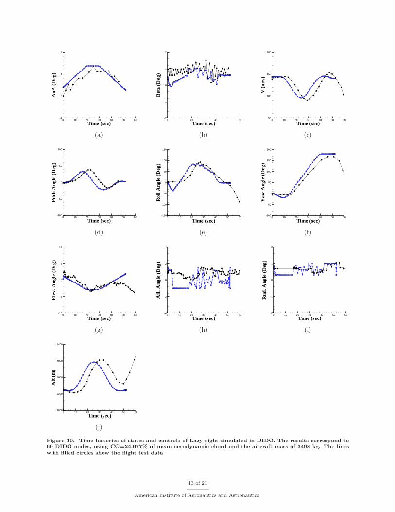
Three manoeuvres are generated. The first is the lazy eight (Fig. 9-a). The aircraft performs a climbingand rolling followed by a diving turn until the final aircraft heading is 180o changed from the initial heading.

A manoeuvre is defined in DIDO using the available experimental tables. The aircraft is allowed to rollfrom 0o to 90o. The manoeuver is initiated from a straight and wing level position, then starts a climb whileincreasing the roll and yaw angles at the same time. Near the maximum altitude, the roll angle has reached90o and then the aircraft starts to dive with rolling towards the left wing. The heading is still increasinguntil it reaches 180o and the aircraft is back to the initial altitude, velocity and the roll angle.

10 of 21


AOA (DEG)

∆CL

δele

-10 -5 0 5 10 15-0.3

-0.2

-0.1

0.0

0.1

0.2

0.3

δele = -25 DEG

δele = 15 DEG

AOA (DEG)

∆CD

δele

-10 -5 0 5 10 15-0.04

-0.02

0.00

0.02

0.04

δele = -25 DEG

δele = 15 DEG

AOA (DEG)

∆Cm

δele

-10 -5 0 5 10 15-0.6

-0.4

-0.2

0.0

0.2

0.4

0.6

δele = -25 DEG

δele = 15 DEG

AOA (DEG)

∆Cnδ

ail

-10 -5 0 5 10 15-0.100

-0.050

0.000

0.050

0.100

Elevator control effectiveness Aileron control effectiveness

AOA (DEG)

∆Cnδ

rud

-10 -5 0 5 10 15-0.05

0.00

0.05

Rudder control effectiveness

Figure 8. Control tables at M=0.25. The deflection angle for aileron and rudder is nine degrees. The circlesdenote experiments.

11 of 21


(a) Lazy Eight (b) Barrel Roll

(c) Immelmann Turn

Figure 9. Manoeuvres generated using DIDO and experimental aero data. The aircraft to the flight path scalein the barrel roll and lazy eight is 100:1. For the Immelmann Turn this is 50:1

12 of 21


Time (sec)

AoA

(Deg

)

0 10 20 30 40 50 60-4

0

4

8

Time (sec)

Bet

a(D

eg)

0 20 40 60-2

-1

0

1

2

Time (sec)

V(m

/s)

0 10 20 30 40 50 6050

100

150

200

(a) (b) (c)

Time (sec)

Pitc

hA

ngle

(Deg

)

0 10 20 30 40 50 60-100

-50

0

50

100

Time (sec)

Rol

lAng

le(D

eg)

0 10 20 30 40 50 60-150

-100

-50

0

50

100

150

Time (sec)

Yaw

Ang

le(D

eg)

0 10 20 30 40 50 60-100

-50

0

50

100

150

200

(d) (e) (f)

Time (sec)

Ele

v.A

ngle

(Deg

)

0 10 20 30 40 50 60-10

-5

0

5

10

Time (sec)

Ail.

Ang

le(D

eg)

0 10 20 30 40 50 60-4

-2

0

2

4

Time (sec)

Rud

.Ang

le(D

eg)

0 10 20 30 40 50 60-2

-1

0

1

2

(g) (h) (i)

Time (sec)

Alt

(m)

0 10 20 30 40 50 602800

3200

3600

4000

4400

(j)

Figure 10. Time histories of states and controls of Lazy eight simulated in DIDO. The results correspond to60 DIDO nodes, using CG=24.077% of mean aerodynamic chord and the aircraft mass of 3498 kg. The lineswith filled circles show the flight test data.

13 of 21


An optimal solution is found and the results are shown against flight test data in Fig. 10. The simulationresults closely follow the trend of flight test data.

Next, for a barrel roll (Fig. 9-b) the aircraft performs a complete rotation around its longitudinal axis.For a barrel roll to the left, the manoeuver is initiated by a pitch up and a roll turn to the left. Duringthis part of the flight, the left wing is the lowest wing, while the aircraft yaws to the left. At the maximumaltitude, the aircraft is nearly upside down. During the second half of the roll, the right wing is lowest andthe aircraft tends to yaw to the right.

Again DIDO was used to re-generate the manoeuvre. The roll test angles are in the range of [-180o,180o]. The aircraft is initially straight and wing level, then starts a roll turn, while climbing at the sametime. Near the maximum altitude, the roll angle has reached -180o, i.e. the aircraft is upside down. Next,the aileron is gradually relaxed to complete the turn by bringing the roll angle again to zero.

The starting speed and altitude of the minimum time manoeuver are set to 158 ms−1 and 6076 m,respectively. Also, the angles of attack should not exceed the upper limit of 12 degrees. The elevator, aileronand rudder deflection values are also limited to the upper and lower values given in flight test data. Anoptimal solution was found and the results are shown against flight test data in Fig. 11. The results showthat the optimal solution resembles the flight test data. The main differences are probably due to settingtake-off moments of inertia for this manoeuvre.

The Immelmann turn, a combined roll and loop manoeuvre, is initiated with a pitch up flight at theentry, and then continues to pull back on the controls such that the aircraft draws a loop in the longitudinalplane. The rudder and ailerons are deflected in a way that the half-loop becomes straight when viewed fromthe ground. At the end of this loop, the aircraft is upside down, then the aileron(s) is applied to execute ahalf-roll turn to correct the aircraft orientation. The manoeuvre is terminated at a higher altitude and a 180degrees reversion of heading. The initial flight speed plays an essential role to accomplish this manoeuvre.

Based on available flight test data, an Immelmann turn manoeuvre is defined. The simulated manoeuvrechanges the heading of the aircraft from 0 to 1800, while the final values of the velocity and latitude (x) arefixed with those at the initial time. The starting speed and altitude of the minimum time manoeuver areset to 163.57 ms−1 and 2986m, respectively. Also the angles of attack should not exceed the upper limit of12 degrees. The elevator, aileron and rudder deflection values are also limited to the upper and lower valuesgiven in flight test data. The final manoeuvre is shown in Fig. 12 plotted against flight test data.

The results show that predicted values of altitude, aircraft flight speed and Euler angles match wellwith flight test data. Although the general trends of angle of attack and elevator deflection are also closelycaptured using DIDO time-optimal solution, the elevator oscillates at initial steps and there is a discrepancyat final values. High frequency values are seen for the aileron and rudder deflections.

The Immelmann turn contains an inherent discontinuity point. During the upward trajectory and beforethe pitch angle of the aircraft hits the maximum allowed angle of 90o, the heading and bank angles remainvirtually constant. Just after the maximum pitch angle point, the aircraft orientation is suddenly reversed,resulting in a sharp jump of the heading and bank angle values at this point. The presence of discontinuitiesincurs serious theoretical and numerical difficulties for the optimal control problem.?,? The implementationof standard direct pseudospectral(PS) method for the trajectory optimization problems with the jump dis-continuities in the states exhibit an over-shoot of predictions at the jump, named Gibbs phenomenon. Insuch a case, the nodes refinement might lead to inefficiencies and an ill-conditioned problem.

The step discontinuity is seen around t = 20 seconds. The lateral predictions are influenced by thepresence of this discontinuity. Very small amplitude Gibbs oscillations are recorded at the yaw and rollangles, however the impacts are much larger for predicted values of side-slip angle and surface deflection ofrudder and aileron.

C. Replay of Manoeuvres

The unsteady Euler solver was applied to the DIDO solution in order to evaluate direct aerodynamic coeffi-cients. The predictions were compared against aerodynamic forces from the tabular model. The comparisonstest the CFD formulation of the manoeuvre replay, which is done in a time accurate fashion with controlsurface deflections. The lateral force and moment coefficients are small for the studied manoeuvres, here,only longitudinal forces and moment are compared.

In all cases, the full aircraft geometry was used with the grid scaling of 1.0. A converged steady-statesolution was used as the starting condition. These conditions correspond to the initial point (t = 0) of eachmanoeuvre. The physical time step correspond to the number of nodes used in the optimal code, DIDO.

14 of 21


Time (sec)

AoA

(Deg

)

0 10 20 30 40 50 60-5

0

5

10

Time (sec)

Bet

a(D

eg)

10 20 30 40 50 60-2

-1

0

1

2

Time (sec)

V(m

/s)

0 10 20 30 40 50 6050

100

150

200

(a) (b) (c)

Time (sec)

Pitc

hA

ngle

(Deg

)

0 10 20 30 40 50 60-60

-40

-20

0

20

40

60

Time (sec)

Rol

lAng

le(D

eg)

0 10 20 30 40 50 60-400

-300

-200

-100

0

100

200

Time (sec)

Yaw

Ang

le(D

eg)

0 10 20 30 40 50 600

50

100

150

(d) (e) (f)

Time (sec)

Ele

v.A

ngle

(Deg

)

0 10 20 30 40 50 60-6

-4

-2

0

2

4

6

Time (sec)

Ail.

Ang

le(D

eg)

0 10 20 30 40 50 60-6

-4

-2

0

2

4

6

Time (sec)

Rud

.Ang

le(D

eg)

0 10 20 30 40 50 60-2

-1

0

1

2

(g) (h) (i)

Time (sec)

Alt

(m)

0 10 20 30 40 50 60

6000

6500

7000

(j)

Figure 11. Time histories of states and controls of Barrel roll simulated in DIDO. The results correspond to60 DIDO nodes, using CG=24.297% of mean aerodynamic chord and the aircraft mass of 3653 kg. The lineswith filled circles show the flight test data.

15 of 21


Time (sec)

AoA

(Deg

)

0 10 20 30 40-4

0

4

8

12

Time (sec)

Bet

a(D

eg)

0 10 20 30 40-4

-2

0

2

4

Time (sec)

V(m

/s)

0 10 20 30 4050

100

150

200

(a) (b) (c)

Time (sec)

Pitc

hA

ngle

(Deg

)

0 10 20 30 40-100

0

100

Time (sec)

Rol

lAng

le(D

eg)

0 10 20 30 40-50

0

50

100

150

200

Time (sec)

Yaw

Ang

le(D

eg)

0 10 20 30 40-50

0

50

100

150

200

(d) (e) (f)

Time (sec)

Ele

v.A

ngle

(Deg

)

0 10 20 30 40-10

-5

0

5

10

Time (sec)

Ail.

Ang

le(D

eg)

0 10 20 30 40-5

0

5

10

Time (sec)

Rud

.Ang

le(D

eg)

0 10 20 30 40-1

0

1

2

(g) (h) (i)

Time (sec)

Alt

(m)

0 10 20 30 402800

3200

3600

4000

4400

(j)

Figure 12. Time histories of states and controls of Immelmann Turn simulated in DIDO. The results correspondto 60 DIDO nodes, using CG=24.265% of mean aerodynamic chord and the aircraft mass of 3629 kg. Thelines with filled circles show the flight test data.

16 of 21


The CFD solver time is found from scaling the physical time based on the grid reference length and thereference velocity. The number of the time step was set to ns = 5000 that has a uniform stepping from t1to tns . The aircraft reference point velocity at each time step was defined from the initial conditions andthe interpolation of DIDO solution. The surface-volume solutions and the body-axis forces and momentscomputed at each CFD time step are available.

The first manoeuvre presented is the Lazy-Eight. Based on the time histories of the DIDO solution, thevalues of aircraft reference point velocity, va at each time step was defined. The initial steady state velocity,v0, was set to 143 m/s. The steady state solution has 1.6 degree angle of attack obtained from the initialpoint of the manoeuvre. The tabular and replay values for the lift, drag and pitching moment are comparedin Fig. 13. The results show that the tables are in perfect agreement with the replay solution. Duringthe manoeuvre the angle of attack remains below six degrees with a maximum Mach number of 0.44. Thisaircraft has no time hysteresis at such a conditions and as expected the tables perfectly match the directsolution from the replay.

Time (sec)

CL

0 10 20 30 40 500

0.4

0.8

1.2

Time (sec)

CD

0 10 20 30 40 500.00

0.01

0.02

0.03

0.04

0.05

Time (sec)

Cm

0 10 20 30 40 50-0.4

-0.2

0

0.2

Figure 13. Lazy-Eight replay solution. The solid line shows the replay simulation.

The second manoeuvre considered is the Barrel-roll. The initial steady conditions are: v0 = 159 m/s andan angle of attack of 1.9 degrees. From the DIDO solution, the grid point locations and grid point velocitiesare set. The tabular and replay values for the lift, drag and pitching moment are compared in Fig. 14. Theresults show good agreement with the replay solution. The angle of attack during manoeuvre time remainsbelow eight degrees, while a good agreement is expected between the tables and the replay.

Finally, the results of the Immelmann turn are presented in Fig. 15. The initial steady conditions are:v0 = 164 m/s and AOA=0.06. The trends of lift, drag and pitching moment closely follow the replay withsome localized differences between the replay and tabular values. There are no history effects from the stateparameters since the aircraft flies in aerodynamically benign regions of the flight envelope. The differencesare mainly due to dynamic effects from the very rapid motion of the control surfaces. As discussed earlier,the Immelmann turn contains an inherent discontinuity point and results in the time optimal solution having

17 of 21


Time (sec)

CL

0 10 20 30 40 500

0.4

0.8

1.2

Time (sec)

CD

0 10 20 30 40 500.00

0.02

0.04

0.06

0.08

0.10

Time (sec)

Cm

0 10 20 30 40 50-0.4

-0.2

0

0.2

Figure 14. Barrel Roll replay solution. The solid line shows the replay simulation.

18 of 21


high frequency and large amplitude motion of the control surfaces. The effects of rapid motion of the controlsurface have been discussed in a paper by Ghoreyshi et al.20

Time (sec)

CL

0 5 10 15 20-0.2

0.0

0.2

0.4

0.6

0.8

1.0

1.2

Time (sec)

CD

0 5 10 15 200.00

0.06

0.12

0.18

Time (sec)

Cm

0 5 10 15 20-1.2

-0.8

-0.4

0.0

0.4

Figure 15. The Immelmann turn replay solution. The solid line shows the replay simulation.

V. Conclusions

The paper investigate the validity of the tabular approach for the maneuvering aircraft by testing theaerodynamic model through replaying manoeuvres using an unsteady CFD calculation to check the consis-tency of the aerodynamic forces and moments. The CFD solver uses two types of mesh movement, namelyrigid motion, and transfinite interpolation for the control surfaces.

The Euler equations were used to demonstrate the replay framework. Sampling and Data fusion was usedto allow the generation of the aerodynamic tables in a feasible number of CFD calculations. The validationagainst available experimental data showed the solutions are credible for the shock effects, but they fail topredict the drag force and lateral coefficients due to lack of skin friction.

Three aerobatic manoeuvres were generated using the time-optimal solver, DIDO. The results werecompared with available flight test data. The trajectories of both simulation and test data match well forall cases. In terms of control values, the Immelmann turn simulation includes high frequency motion of thesurface deflections, due to the presence of a discontinuity point in the roll angle. The time-optimal solverfor the trajectory optimization experiences problems with the jump discontinuities in the states due to anover-shoot of predictions at the jump from the Gibbs phenomenon. This results in the formation of spikesin the replay solutions due to dynamic effects from the very rapid motion of the control surfaces.

The results of tabular predictions were compared against the coefficients from the replaying the manoeuvreusing an unsteady CFD calculation. For all considered manoeuvres the aircraft flies in aerodynamicallybenign regions of the flight envelope and the tables perfectly match the replay solution. The results of

19 of 21


this paper demonstrated the validity of using tables for such conditions. Overall, the paper illustrates thevalidity of the CFD framework for generating aerodynamic tables and replaying manoeuvres to test them.This framework, when applied to more demanding manoeuvres can show the limitations in the tabularformulation.

VI. Acknowledgements

Computer time for RANS calculations was provided through the UK Applied Aerodynamics Consortium(UKAAC) under Engineering and Physical Sciences Research Council grant EP/F005954/1. This work waspartly done under funding from the European Union sixth framework project SimSAC (Simulating Stabilityand Control).

References

1Bryan, G. H. and Williams, W. E., ”The Longitudinal Stability Of Aerial Gliders”, 1904, Proceceeding of Royal Society,London, Vol. 33, Series A., pp. 100-116

2Greenwell, D. I., ”A Review of Unsteady Aerodynamic Modelling for Flight Dynamics of Manoeuvrable Aircraft”, 2004,AIAA 2004-5276, AIAA Atmospheric Flight Mechanics Conference and Exhibit, 16 - 19 August, Providence, Rhode Islandm

3Hamel, P. G. and Jategaonkar, R. V., Evolution of Flight Vehicle System Identification, Journal of Aircraft, Vol. 33, No.1, 1996, pp. 9-28

4Jouannet, C. and Krus, P., Lift Coefficient Predictions for Delta Wing Under Pitching Motions, 32nd AIAA FluidDynamics Conference and Exhibit AIAA-2002-2969, 24-26 June 2002, St. Louis, Missouri

5Katz, J. and Schiff, L. B., ”Modeling Aerodynamic Responses to Aircraft Maneuvers A Numerical Validation”, Journalof Aircraft, 1986, Vol. 23, No. 1, pp. 19-25

6Tobak, M. and Schiff, L.B., Aerodynamic Mathematical Modeling: Basic Concepts, AGARD Lecture Series on DynamicStability Parameters, Lecture No. 1, March 1981.

7Tobak, M., Chapman, G. T., and Schiff, L. B., ”Mathematical Modeling of the Aerodynamic Characteristics in FlightDynamics”, 1984, NASA technical report, TM 85880.

8Goman, M. and Khrabrov, A., ”State-Space Representation of Aerodynamic Characteristics of an Aircraft at High Anglesof Attack”, 1992, AIAA Paper 92-4651-CP.

9Klein, V. and Nodere, K. D., ”Modeling of Aircraft Unsteady Aerodynamic Characteristics”, 1994, NASA technicalreport, National Aeronautics and Space Administration Langley Research Center Hampton, Virginia, 23681-0001

10Rudnik, R. and Germain, E., ”Re-No. Scaling Effects on the EUROLIFT High Lift Configurations”, 2007, 45th AIAAAerospace Sciences Meeting and Exhibit, AIAA 2007-752, January 2007, Reno, Nevada

11Jirasek, A., Jeans, T. L., Martenson, M., Cummings, R. M. and Bergeron, K., ”Improved Methodologies for ManeuverDesign of Aircraft Stability and Control Simulations”, 2010, 48th AIAA Aerospace Sciences Meeting Including the New HorizonsForum and Aerospace Exposition, AIAA 2010-515, January 2010, Orlando, Florida

12Da Ronch,A. , Valespin, D., Ghoreyshi, M. and Badcock. K. J., ”Computation and Evaluation of Dynamic Derivativesusing CFD”, 2010, AIAA-2010-4817 28th AIAA Applied Aerodynamics Conference, Chicago, Illinois, June 28-1

13Da Ronch, A., Ghoreyshi, M., Badcock, K. J., Gortz, S., Widhalm, M. and Dwight, R. ”Linear Frequency Domain andHarmonic Balance Predictions of Dynamic Derivatives ”, 2010, AIAA-2010-4699, 28th AIAA Applied Aerodynamics Conference,Chicago, Illinois, June 28-1.

14Ballhaus, W.F. and Goorjian, P.M., Computation of Unsteady Transonic Flow by the Indicial Method, AIAA Journal,Vol. 16, 1978, pp. 117-124.

15Rizzetta, D.P., Time-Dependent Response of a Two-Dimensional Airfoil in Transonic Flow, AIAA Journal, Vol. 17, 1979,pp. 26-32.

16Chyu, W.J. and Schiff, L.B., Nonlinear Aerodynamic Modeling of Flap Oscillations in Transonic Flow: A NumericalValidation, AIAA Journal, Vol. 21, 1983, pp. 106-113.

17Steger, J.L. and Bailey, H.E., Calculation of Transonic Aileron Buzz, AIAA Journal, Vol. 18, 1980, pp. 249-255.18Allan, M.R., Badcock, K. J. and Richards, B. E., CFD Based Simulation of Longitudinal Flight Mechanics With Control.

43rd AIAA Aerospace Science Meeting and Exhibition, AIAA-2005-46.19Schutte,A. , Einarsson, G., Raichle,A., Schoning,B., Mnnich, W. and Forkert, T., Numerical Simulation of Manoeuvreing

Aircraft by Aerodynamic, Flight Mechanics, and Structural Mechanics Coupling, Journal of Aircraft Vol. 46, No. 1, 2009, pp.53 -64

20Ghoreyshi, M., Badcock, K., Da Ronch, A., Swift, A., Marques, S. and Ames, N., ”Framework for Establishing theLimits of Tabular Aerodynamic Models for Flight Dynamics Analysis ”, 2009, AIAA-2009-6273, AIAA Guidance, Navigation,and Control Conference, Chicago, Illinois, Aug. 10-13.

21Ghoreyshi, M., Badcock, K. J. and Woodgate, M., Accelerating the Numerical Generation of Aerodynamic Models forFlight Simulation, Journal of Aircraft, Vol. 46, No. 3, pp. 972- 980

22Badcock, K.J., Richards, B.E. and Woodgate, M.A. Elements of Computational Fluid Dynamics on Block StructuredGrids using Implicit Solvers. Progress in Aerospace Sciences, vol 36, 2000, pp 351-392.

23Boelens, O.J., Badcock, K.J., Elmilgui, A., Abdol-Hamid, K.S. and Massey, S.J., Comparison of Measured and BlockStructured Simulation Results for the F-16XL Aircraft, Journal of Aircraft, 46(2), March, 2009, 377-384.

20 of 21


24von Kaenel,R., Rizzi, A., Oppelstrup, J., Goetzendorf-Grabowski, T., Ghoreyshi, M., Cavagna, L. and Berard, A.,”CEASIOM: Simulating Stability & Control with CFD/CSM in Aircraft Conceptual Design”, 2008, 26th International Congressof the Aeronautical Sciences, ICAS.

25Betts, J. T., Survey of Numerical Methods for Trajectory Optimization, 1998, Journal of Guidance, Control, and Dy-namics, Vol. 21, No. 2, pp. 193 207.

26Hull, D. G., Conversion of Optimal Control Problems into Parameter Optimization Problems, 1997, Journal of Guidance,Control, and Dynamics, Vol. 20, No. 1, pp. 5760.

27Brinkman, K. and Visser, H. G. , Optimal turn-back manoeuvre after engine failure in a single-engine aircraft duringclimb-out, Journal of Aerospace Engineering, Vol. 22, Part G., 2006,pp. 17-27

28Ross, I. M., and Fahroo, F., ”Users Manual for DIDO 2002: A MATLAB Application Package for Dynamic Optimization,”2002, NPS Technical Rept, Dept. of Aeronautics and Astronautics, Naval Postgraduate School, Monterey, CA, AA-02-002.

29The Mathworks, Inc. , MATLAB version 2008a, Inc. http://www.mathworks.com, 200830Gottlieb, D., Hussaini, M. Y., and Orszag, S. A., Theory and Applications of Spectral Methods, 1984, Spectral Methods

for PDEs, Society for Industrial and AppliedMathematics, Philadelphia.31Canuto, C., Hussaini, M. Y., Quarteroni, A., and Zang, T. A., ”Spectral Methods in Fluid Dynamics”, 1988, Springer-

Verlag, New York, 1988.32Elnagar, J., Kazemi, M. A., and Razzaghi, M., The Pseudospectral Legendre Method for Discretizing Optimal Control

Problems, 1995, IEEE Transactions on Automatic Control, Vol. 40, No. 10, pp. 1793 1796.33Etkin, B., Dynamics of Flight, Stability and Control, 2nd Edition, Wiley, 198234Steven, B.L. and Lewis, F. L., Aircraft Control and Simulatoon, Wiley, 199235Rampurawala, A.M. and Badcock, K.J., Evaluation of a Simplified Grid Treatment for Oscillating Trailing-Edge Control

Surfaces, Journal of Aircraft, 44(4), 2007, 1177-1188.36Roskam, J., ” Airplane Design. Part I through VIII”, 1990, Roskam Aviation and Engineering Corporation, Kansas,

USA.37Homescu, C. and Navon, I. M., ”Optimal control of flow with discontinuities”, 2003, Journal of Computatational Physics,

Vol. 187 pp. 660682.38Ross, I. M., Fahroo, F., ”Pseudospectral Knotting Methods for Solving Optimal Control Problem”, 2004, Journal of

Guidance, Control, and Dynamics Vol. 27, No. 3, pp. 397-405

21 of 21


simulation of aircraft manoeuvres based on computational...

Documents