LUND UNIVERSITY

PO Box 117221 00 Lund+46 46-222 00 00

Simulation of a Pneumatic Hybrid Powertrain with VVT in GT-Power and Comparisonwith Experimental Data

Trajkovic, Sasa; Tunestål, Per; Johansson, Bengt

Published in:SAE Technical Paper Series

Published: 2009-01-01

Link to publication

Citation for published version (APA):Trajkovic, S., Tunestål, P., & Johansson, B. (2009). Simulation of a Pneumatic Hybrid Powertrain with VVT inGT-Power and Comparison with Experimental Data. In SAE Technical Paper Series Society of AutomotiveEngineers.

General rightsCopyright and moral rights for the publications made accessible in the public portal are retained by the authorsand/or other copyright owners and it is a condition of accessing publications that users recognise and abide by thelegal requirements associated with these rights.

• Users may download and print one copy of any publication from the public portal for the purpose of privatestudy or research. • You may not further distribute the material or use it for any profit-making activity or commercial gain • You may freely distribute the URL identifying the publication in the public portal

Take down policyIf you believe that this document breaches copyright please contact us providing details, and we will removeaccess to the work immediately and investigate your claim.

Download date: 06. Sep. 2018

The Engineering Meetings Board has approved this paper for publication. It has successfully completed SAE’s peer review process under the supervision of the session organizer. This process requires a minimum of three (3) reviews by industry experts. All rights reserved. No part of this publication may be reproduced, stored in a retrieval system, or transmitted, in any form or by any means, electronic, mechanical, photocopying, recording, or otherwise, without the prior written permission of SAE. ISSN 0148-7191 Positions and opinions advanced in this paper are those of the author(s) and not necessarily those of SAE. The author is solely responsible for the content of the paper. SAE Customer Service: Tel: 877-606-7323 (inside USA and Canada) Tel: 724-776-4970 (outside USA) Fax: 724-776-0790 Email: CustomerService@sae.org SAE Web Address: http://www.sae.org

Printed in USA

2009-01-1323

Simulation of a Pneumatic Hybrid Powertrain with VVT in GT-Power and Comparison with Experimental Data

Sasa Trajkovic, Per Tunestål and Bengt Johansson Division of Combustion Engines, Lund University, Faculty of Engineering

Copyright © 2009 SAE International

ABSTRACT

In the study presented in this paper, experimental data from a pneumatic hybrid has been compared to the results from a simulation of the engine in GT-Power. The engine in question is a single-cylinder Scania D12 diesel engine, which has been converted to work as a pneumatic hybrid. The base engine model, provided by Scania, is made in GT-Power and it is based on the same engine configuration as the one used during real engine testing.

During pneumatic hybrid operation the engine can be used as a 2-stroke compressor for generation of compressed air during vehicle deceleration and during vehicle acceleration the engine can be operated as a 2-stroke air-motor driven by the previously stored pressurized air. There is also a possibility to use the stored pressurized air in order to supercharge the engine when there is a need for high torque, like for instance at take off after a standstill or during an overtake maneuver. Previous experimental studies have shown that the pneumatic hybrid is a promising concept and a possible competitor to the electric hybrid.

This paper consists mainly of two parts. The first one describes an attempt to recreate the real engine as a computer model with the aid of the engine simulation software GT-power. A model has been created and the results have been validated against real engine data. The second part describes a parametric study where different parameters and their effect on pneumatic hybrid performance have been investigated.

INTRODUCTION

Growing environmental concerns, together with higher fuel prices, has created a need for cleaner and more efficient alternatives to the propulsion systems of today. Currently, the majority of all vehicles are equipped with combustion engines having a maximum thermal efficiency of 30-40%. The average efficiency is much lower, especially during city driving since it involves frequent starts and stops.

Today there are several solutions to meet the demand for better fuel economy and one of them is electric hybrids. The idea with electric hybridization is to reduce the fuel consumption by taking advantage of the, otherwise lost, brake energy. Hybrid operation in combination with engine downsizing can also allow the combustion engine to operate at its best operating points in terms of load and speed.

The main drawbacks with electric hybrids are that they require an additional propulsion system and large heavy batteries with a limited life-cycle. This introduces extra manufacturing costs which are compensated by a higher end-product price.

One way of keeping the extra hybridization cost as low as possible compared to a conventional vehicle, is the introduction of the pneumatic hybrid. It does not require an expensive extra propulsion source and it works in a way similar to the electric hybrid. During deceleration of the vehicle, the engine is used as a compressor that converts the kinetic energy contained in the vehicle into energy in the form of compressed air which is stored in a pressure tank. After a standstill the engine is used as an air-motor that utilizes the pressurized air from the tank in

order to accelerate the vehicle. During a full stop the engine can be shut off.

In this study, a model of the pneumatic hybrid engine has been created with the intent to further explore its potential and characteristics. Previous experimental studies [1, 2] have shown that different factors, like for instance tank valve head diameter and valve timings, play an important role in the overall pneumatic hybrid performance. While it is time consuming to change the tank valve head diameter on a real engine, it can be done within seconds on a computer model. Therefore a real engine based computer model can serve as a tool in order to more easily find optimal engine parameters.

PNEUMATIC HYBRID

Pneumatic hybrid operation introduces new operating modes in addition to conventional internal combustion engine (ICE) operation. The main idea with pneumatic hybrid is to use the ICE in order to compress atmospheric air and store it in a pressure tank when decelerating the vehicle. The stored compressed air can then be used either to accelerate the vehicle or to supercharge the engine in order to achieve higher loads when needed. The pneumatic hybrid also makes it possible to completely shut off the engine at idling like for instance at a stoplight, which in turn contributes to lower fuel consumption. [3,4,5,6]

In this study a single-cylinder engine was used. In reality, in for instance a heavy duty truck, one cylinder will not be enough to take full advantage of the pneumatic hybrid. A pneumatic hybrid will most probably utilize multiple cylinders. The number of cylinders that will be converted for pneumatic hybrid operation for a certain vehicle is hard to estimate at this point. It depends on, among other things, the vehicle weight and the maximum braking torque needed.

MODES OF ENGINE OPERATION

The main pneumatic hybrid vehicle operations are compressor mode (CM) and air-motor mode (AM).

COMPRESSOR MODE

In compressor mode (CM) the engine is used as a 2-stroke compressor in order to decelerate the vehicle. The kinetic energy of the moving vehicle is converted to potential energy in the form of compressed air.

During CM the inlet valve opens a number of crank angle degrees (CAD) after top dead centre (ATDC) and brings fresh air to the cylinder, and closes around bottom dead centre (BDC). The moving piston starts to compress the air contained in the cylinder after BDC and the tank valve opens somewhere between BDC and TDC, depending on how much braking torque is needed, and closes shortly after TDC. The compressed air

generated during CM is stored in a pressure tank that is connected to the cylinder head.

AIR-MOTOR MODE

In air-motor mode (AM) the engine is used as a 2-stroke air-motor that uses the compressed air from the pressure tank in order to accelerate the vehicle. The potential energy in the form of compressed air is converted to mechanical energy on the crankshaft which in the end is converted to kinetic energy.

During AM the tank valve opens at TDC or shortly after and the compressed air fills the cylinder to give the torque needed in order to accelerate the vehicle. Somewhere between TDC and BDC the tank valve closes, depending on how much torque the driver demands. Increasing the tank valve duration will increase the torque generated by the compressed air. The inlet valve opens around BDC in order to allow the compressed air to escape from the cylinder.

EXPERIMENTAL SETUP

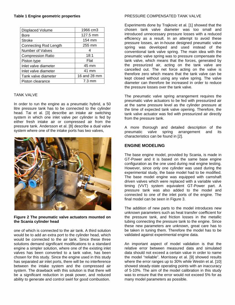
The engine used in this study can be seen in Figure 1. It is a 6-cylinder Scania D12 diesel engine converted to a single-cylinder engine. The engine is equipped with a pneumatic-electric fully variable valve actuating system which has been more thoroughly described by Trajkovic et al. [7]. The geometric properties of the engine can be seen in Table 1. Figure 2 shows a close-up of the pneumatic valve actuators mounted on top of the Scania cylinder head.

Figure 1 The engine used in this study

The exhaust valves were deactivated throughout the whole study because no fuel was injected and thus there was no need for exhaust gas venting.

PRESSURE COMPENSATED TANK VALVE Table 1 Engine geometric properties

Experiments done by Trajkovic et al. [1] showed that the chosen tank valve diameter was too small and introduced unnecessary pressure losses with a reduced efficiency as a result. In an attempt to avoid these pressure losses, an in-house designed pneumatic valve spring was developed and used instead of the conventional tank valve spring. The main idea with the pneumatic valve spring was to pressure compensate the tank valve, which means that the forces, generated by the pressurized air, acting on the tank valve are cancelled out. The net force acting on the valve is therefore zero which means that the tank valve can be kept closed without using any valve spring. The valve diameter can therefore be increased in order to reduce the pressure losses over the tank valve.

Displaced Volume 1966 cm3 Bore 127.5 mm Stroke 154 mm Connecting Rod Length 255 mm Number of Valves 4 Compression Ratio 18:1 Piston type Flat Inlet valve diameter 45 mm Inlet valve diameter 41 mm Tank valve diameter 16 and 28 mm Piston clearance 7.3 mm

TANK VALVE The pneumatic valve spring arrangement requires the pneumatic valve actuators to be fed with pressurized air at the same pressure level as the cylinder pressure at the time of expected tank valve opening. Therefore, the tank valve actuator was fed with pressurized air directly from the pressure tank.

In order to run the engine as a pneumatic hybrid, a 50 litre pressure tank has to be connected to the cylinder head. Tai et al. [3] describe an intake air switching system in which one inlet valve per cylinder is fed by either fresh intake air or compressed air from the pressure tank. Andersson et al. [8] describe a dual valve system where one of the intake ports has two valves,

A more thorough and detailed description of the pneumatic valve spring arrangement and its characteristics can be found in [2].

ENGINE MODELING

The base engine model, provided by Scania, is made in GT-Power and it is based on the same base engine configuration as the one used during real engine testing. However, since only one cylinder was used during the experimental study, the base model had to be modified. The base model engine was equipped with camshaft driven valves which were replaced with a variable valve timing (VVT) system equivalent GT-Power part. A pressure tank was also added to the model and connected to one of the inlet ports of the engine. The final model can be seen in Figure 3.

The addition of new parts to the model introduces new unknown parameters such as heat transfer coefficient for the pressure tank, and friction losses in the metallic tubing connecting the pressure tank to the engine. Since these new parameters are unknown, great care has to be taken in tuning them. Therefore the model has to be validated against experimental engine data.

Figure 2 The pneumatic valve actuators mounted on the Scania cylinder head

one of which is connected to the air tank. A third solution would be to add an extra port to the cylinder head, which would be connected to the air tank. Since these three solutions demand significant modifications to a standard engine a simpler solution, where one of the existing inlet valves has been converted to a tank valve, has been chosen for this study. Since the engine used in this study has separated air inlet ports, there will be no interference between the intake system and the compressed air system. The drawback with this solution is that there will be a significant reduction in peak power, and reduced ability to generate and control swirl for good combustion.

An important aspect of model validation is that the relative error between measured data and simulated data should not exceed a certain value in order to name the model “reliable”. Morrissey et al. [9] showed results where the error ranges up to 30% while Westin et al. [10] showed steady-state operating points with an inaccuracy of 5-10%. The aim of the model calibration in this study was to ensure that the error would not exceed 5% for as many model parameters as possible.

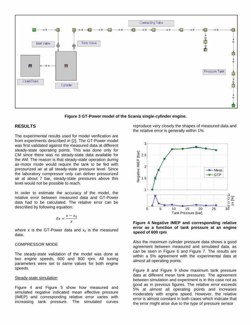
Figure 3 GT-Power model of the Scania single-cylinder engine.

RESULTS

The experimental results used for model verification are from experiments described in [2]. The GT-Power model was first validated against the measured data at different steady-state operating points. This was done only for CM since there was no steady-state data available for the AM. The reason is that steady-state operation during air-motor mode would require the tank to be fed with pressurized air at all steady-state pressure level. Since the laboratory compressor only can deliver pressurized air at about 7 bar, steady-state pressures above this level would not be possible to reach.

In order to estimate the accuracy of the model, the relative error between measured data and GT-Power data had to be calculated. The relative error can be described by following equation:

where x is the GT-Power data and x0 is the measured data.

COMPRESSOR MODE

The steady-state validation of the model was done at two engine speeds, 600 and 900 rpm. All tuning parameters were set to same values for both engine speeds.

Steady-state simulation

Figure 4 and Figure 5 show how measured and simulated negative indicated mean effective pressure (IMEP) and corresponding relative error varies with increasing tank pressure. The simulated curves

reproduce very closely the shapes of measured data and the relative error is generally within 1%.

Figure 4 Negative IMEP and corresponding relative error as a function of tank pressure at an engine speed of 600 rpm

Also the maximum cylinder pressure data shows a good agreement between measured and simulated data, as can be seen in Figure 6 and Figure 7. The results are within a 5% agreement with the experimental data at almost all operating points.

Figure 8 and Figure 9 show maximum tank pressure data at different mean tank pressures. The agreement between simulation and experiment is in this case not as good as in previous figures. The relative error exceeds 5% at almost all operating points and increases moderately with engine speed. However, the relative error is almost constant in both cases which indicate that the error might arise due to the type of pressure sensor

1

1.5

2

2.5

3N

egat

ive

IME

P [b

ar]

MeasGTP

0 5 10 15 20 25 300123

Tank Pressure [bar]

δx [%

]

Figure 5 Negative IMEP and corresponding relative error as a function of tank pressure at an engine speed of 900 rpm

Figure 6 Maximum cylinder pressure and corresponding relative error as a function of tank pressure at an engine speed of 600 rpm

used to measure the port pressure. The sensor in question is a piezoresistive transducer and according to tests done by Tsung et al. [11] the response rate of such transducers are one quarter of the response rate of piezoelectric transducers usually used for in-cylinder pressure measurement. This means that the pressure signal achieved with the piezoresistive transducer is damped and therefore deviates from what would be achieved with a piezoelectric transducer.

The tank valve port temperature can be seen in Figure 10 and Figure 11. The relative error reaches almost 10% at some point which implies that additional calibration needs to be done in order to achieve satisfactory results. The reason why predicted results deviates heavily from measured is that the calibration has mainly been focused on setting the right dimensions of the pipes and connections rather than tuning the heat transfer coefficients and wall temperatures. A greater care in

Figure 7 Maximum cylinder pressure and corresponding relative error as a function of tank pressure at an engine speed of 900 rpm

Figure 8 Maximum tank pressure together with the corresponding relative error at 600 rpm

Figure 9 Maximum tank pressure together with the corresponding relative error at 900 rpm

1

1.5

2

2.5

3

3.5N

egat

ive

IME

P [b

ar]

MeasGTP

0 5 10 15 20 25 30-2024

Tank Pressure [bar]

δx [%

]

0

5

10

15

20

25

Max

Cyl

inde

r Pre

ssur

e [b

ar]

MeasGTP

0 5 10 15 20 25 300

5

Tank Pressure [bar]

δx [%

]

0

5

10

15

20

25

Max

Cyl

inde

r Pre

ssur

e [b

ar]

MeasGTP

0 5 10 15 20 25 300510

Tank Pressure [bar]

δx [%

]

0

5

10

15

20

25

Max

Tan

k P

ress

ure

[bar

]

MeasGTP

0 5 10 15 20 25 300510

Tank Pressure [bar]

δx [%

]

0

5

10

15

20

25

Max

Tan

k P

ress

ure

[bar

]

MeasGTP

0 5 10 15 20 25 306810

Tank Pressure [bar]

δx [%

]

calibration of these parameters would most likely decrease the margin of error. The decline in temperature for the simulated data between tank pressures of 15 and 25 bar indicates that the heat losses in the model are greater compared to measured data.

Transient simulation

During transient engine operation, the valve timings of both the intake and the tank valve are open-loop controlled. The valve timing map has been created from data retrieved during steady-state operation.

Figure 10 Tank valve port temperature and corresponding relative error as a function of tank pressure at an engine speed of 600 rpm

Figure 11 Tank valve port temperature and corresponding relative error as a function of tank pressure at an engine speed of 900 rpm

Figure 12 and Figure 13 show negative IMEP during 800 consecutive cycles of transient engine operation for both simulated and measured values. The agreement of simulated data with measured data is quite good with a relative error mainly within 5 %. However, between 0

and 200 engine cycles, the error exceeds 5 % for both cases. It is difficult to estimate exactly why the simulated data deviates in this way, but one explanation might be poor tuning with respect to heat transfer. The hump-like behavior in Figure 13 in the cycle-interval of 100-200 cycles occurs due to some issues with the pneumatic valve spring arrangement. These issues have been thoroughly discussed in [2]. A behavior like this is quite hard to simulate and therefore there will be some discrepancy between measured and predicted values.

If the results from transient operation are compared with

Figure 12 Negative IMEP and corresponding relative error as a function of engine cycle number during transient CM simulation at an engine speed of 600 rpm

Figure 13 Negative IMEP and corresponding relative error as a function of engine cycle number during transient CM simulation at an engine speed of 900 rpm

those retrieved during steady-state simulations, it can be noticed that transient operation lead to a higher relative error. There might be various possible reasons for such behavior. The most probable reason is that transient gas

350

400

450

500

550

Tank

Val

ve P

ort T

empe

ratu

re [K

]

MeasGTP

0 5 10 15 20 25 30-10010

Tank Pressure [bar]

δx [%

]

350

400

450

500

550

600

650

Tank

Val

ve P

ort T

empe

ratu

re [K

]

MeasGTP

0 5 10 15 20 25 30-10-50

Tank Pressure [bar]

δx [%

]

0

1

2

3

4

Neg

ativ

e IM

EP

[bar

]

MeasGTP

0 200 400 600 800-505

Number of Engine Cycles

δx [%

]0

1

2

3

4

Neg

ativ

e IM

EP

[bar

]

MeasGTP

0 200 400 600 800-505

Number of Engine Cycles

δx [%

]

dynamics differs from those created during stationary conditions and therefore some deviation between the results has to be expected.

Figure 14 and Figure 15 show maximum cylinder pressure data during transient engine operation. During steady-state operation, the GT-Power model over-predicted the maximum cylinder pressure at almost all points. However, during transient operation the model under-predicts the cylinder pressure for almost the entire transient operation interval. Once again this behavior can be attributed to the transient gas dynamics. It can be noticed, that the hump-like behavior seen in the Figure 13 is also visible in Figure 15.

Figure 14 Maximum cylinder pressure and corresponding relative error as a function of engine cycle number during transient CM simulation at an engine speed of 600 rpm

Figure 15 Maximum cylinder pressure and corresponding relative error as a function of engine cycle number during transient CM simulation at an engine speed of 900 rpm

Mean tank pressure data shows a good agreement between measured and simulated data, as can be seen

in Figure 16 and Figure 17. The predicted data is within ±5% of the measured data at both engine speeds.

Comparing Figure 16 and Figure 17 with Figure 8 and Figure 9 indicates that predicted mean tank pressure shows a better agreement with measured data than simulated maximum tank pressure. The reason might be that, due to the nature of the piezoresistive pressure sensor, the signal is somewhat averaged. Therefore, measured maximum tank pressure will differ from real maximum tank pressure. However, since the signal is already averaged, mean tank pressure will show a better agreement with predicted data.

Figure 16 Mean Tank pressure and corresponding relative error as a function of engine cycle number during transient CM simulation at an engine speed of 600 rpm

Figure 17 Mean tank pressure and corresponding relative error as a function of engine cycle number during transient CM simulation at an engine speed of 900 rpm

Figure 18 and Figure 19 show the tank valve port temperature during transient operation at 600 and 900 rpm, respectively. The predicted data deviates

0

5

10

15

20

25

30

Max

Cyl

inde

r Pre

ssur

e [b

ar]

MeasGTP

0 200 400 600 800-10010

Number of Engine Cycles

δx [%

]

0

5

10

15

20

25

30

Max

Cyl

inde

r Pre

ssur

e [b

ar]

MeasGTP

0 200 400 600 800-10010

Number of Engine Cycles

δx [%

]

0

5

10

15

20

25

Mea

n Ta

nk P

ress

ure

[bar

]

MeasGTP

0 200 400 600 800-505

Number of Engine Cycles

δx [%

]

0

5

10

15

20

25

Mea

n Ta

nk P

ress

ure

[bar

]

MeasGTP

0 200 400 600 800-505

Number of Engine Cycles

δx [%

]

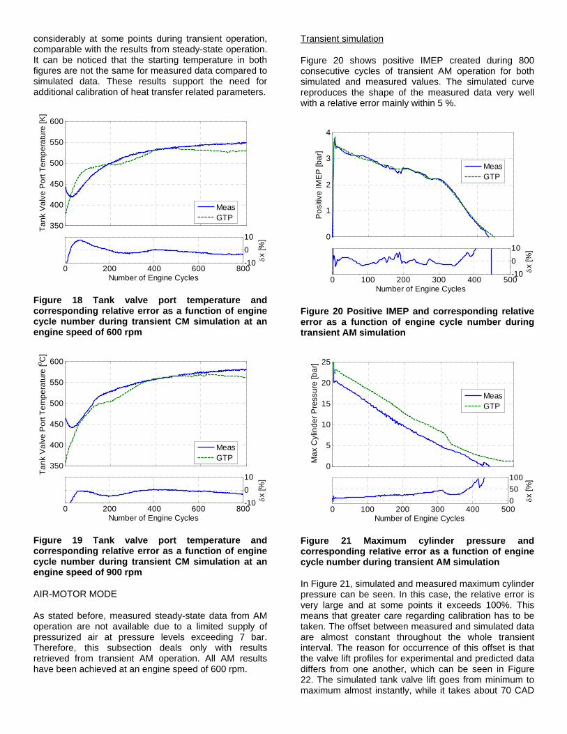
considerably at some points during transient operation, comparable with the results from steady-state operation. It can be noticed that the starting temperature in both figures are not the same for measured data compared to simulated data. These results support the need for additional calibration of heat transfer related parameters.

Figure 18 Tank valve port temperature and corresponding relative error as a function of engine cycle number during transient CM simulation at an engine speed of 600 rpm

Figure 19 Tank valve port temperature and corresponding relative error as a function of engine cycle number during transient CM simulation at an engine speed of 900 rpm

AIR-MOTOR MODE

As stated before, measured steady-state data from AM operation are not available due to a limited supply of pressurized air at pressure levels exceeding 7 bar. Therefore, this subsection deals only with results retrieved from transient AM operation. All AM results have been achieved at an engine speed of 600 rpm.

Transient simulation

Figure 20 shows positive IMEP created during 800 consecutive cycles of transient AM operation for both simulated and measured values. The simulated curve reproduces the shape of the measured data very well with a relative error mainly within 5 %.

Figure 20 Positive IMEP and corresponding relative error as a function of engine cycle number during transient AM simulation

Figure 21 Maximum cylinder pressure and corresponding relative error as a function of engine cycle number during transient AM simulation

In Figure 21, simulated and measured maximum cylinder pressure can be seen. In this case, the relative error is very large and at some points it exceeds 100%. This means that greater care regarding calibration has to be taken. The offset between measured and simulated data are almost constant throughout the whole transient interval. The reason for occurrence of this offset is that the valve lift profiles for experimental and predicted data differs from one another, which can be seen in Figure 22. The simulated tank valve lift goes from minimum to maximum almost instantly, while it takes about 70 CAD

350

400

450

500

550

600

Tank

Val

ve P

ort T

empe

ratu

re [K

]

MeasGTP

0 200 400 600 800-10010

Number of Engine Cycles

δx [%

]

350

400

450

500

550

600

Tank

Val

ve P

ort T

empe

ratu

re [ o C

]

MeasGTP

0 200 400 600 800-10010

Number of Engine Cycles

δx [%

]

0

1

2

3

4

Pos

itive

IME

P [b

ar]

MeasGTP

0 100 200 300 400 500-10010

Number of Engine Cycles

δx [%

]

0

5

10

15

20

25

Max

Cyl

inde

r Pre

ssur

e [b

ar]

MeasGTP

0 100 200 300 400 500050100

Number of Engine Cyclesδx

[%]

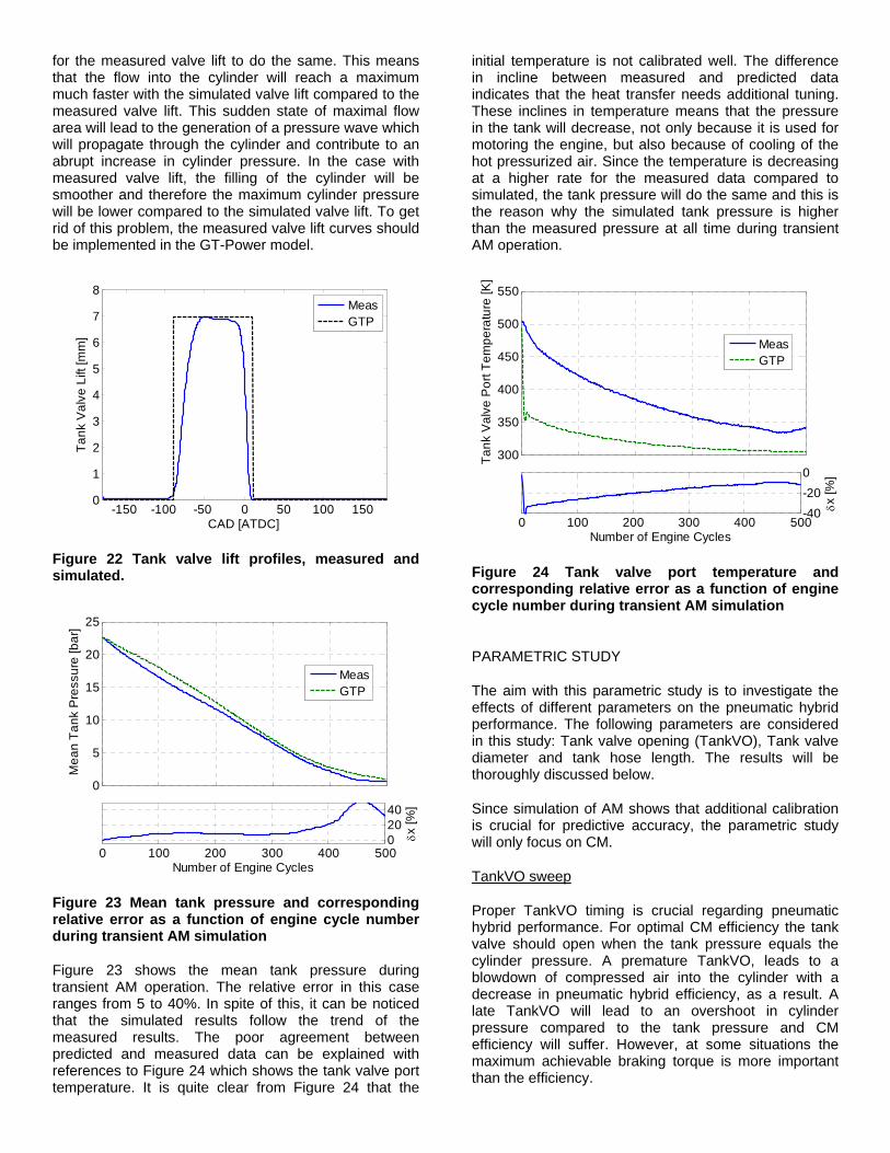
for the measured valve lift to do the same. This means that the flow into the cylinder will reach a maximum much faster with the simulated valve lift compared to the measured valve lift. This sudden state of maximal flow area will lead to the generation of a pressure wave which will propagate through the cylinder and contribute to an abrupt increase in cylinder pressure. In the case with measured valve lift, the filling of the cylinder will be smoother and therefore the maximum cylinder pressure will be lower compared to the simulated valve lift. To get rid of this problem, the measured valve lift curves should be implemented in the GT-Power model.

Figure 22 Tank valve lift profiles, measured and simulated.

Figure 23 Mean tank pressure and corresponding relative error as a function of engine cycle number during transient AM simulation

Figure 23 shows the mean tank pressure during transient AM operation. The relative error in this case ranges from 5 to 40%. In spite of this, it can be noticed that the simulated results follow the trend of the measured results. The poor agreement between predicted and measured data can be explained with references to Figure 24 which shows the tank valve port temperature. It is quite clear from Figure 24 that the

initial temperature is not calibrated well. The difference in incline between measured and predicted data indicates that the heat transfer needs additional tuning. These inclines in temperature means that the pressure in the tank will decrease, not only because it is used for motoring the engine, but also because of cooling of the hot pressurized air. Since the temperature is decreasing at a higher rate for the measured data compared to simulated, the tank pressure will do the same and this is the reason why the simulated tank pressure is higher than the measured pressure at all time during transient AM operation.

Figure 24 Tank valve port temperature and corresponding relative error as a function of engine cycle number during transient AM simulation

PARAMETRIC STUDY

The aim with this parametric study is to investigate the effects of different parameters on the pneumatic hybrid performance. The following parameters are considered in this study: Tank valve opening (TankVO), Tank valve diameter and tank hose length. The results will be thoroughly discussed below.

Since simulation of AM shows that additional calibration is crucial for predictive accuracy, the parametric study will only focus on CM.

TankVO sweep

Proper TankVO timing is crucial regarding pneumatic hybrid performance. For optimal CM efficiency the tank valve should open when the tank pressure equals the cylinder pressure. A premature TankVO, leads to a blowdown of compressed air into the cylinder with a decrease in pneumatic hybrid efficiency, as a result. A late TankVO will lead to an overshoot in cylinder pressure compared to the tank pressure and CM efficiency will suffer. However, at some situations the maximum achievable braking torque is more important than the efficiency.

-150 -100 -50 0 50 100 1500

1

2

3

4

5

6

7

8

CAD [ATDC]

Tank

Val

ve L

ift [m

m]

MeasGTP

0

5

10

15

20

25

Mea

n Ta

nk P

ress

ure

[bar

]

MeasGTP

0 100 200 300 400 50002040

Number of Engine Cycles

δx [%

]

300

350

400

450

500

550

Tank

Val

ve P

ort T

empe

ratu

re [K

]

MeasGTP

0 100 200 300 400 500-40-200

Number of Engine Cycles

δx [%

]

Figure 25 illustrates a TankVO sweep for various steady-state tank pressures at an engine speed of 600 and 900 rpm, respectively. It can clearly be seen how negative IMEP is affected by TankVO timing. The figure shows that there is an optimal TankVO timing for every tank pressure when taking highest efficiency into consideration, where highest efficiency occurs near the minimum in each IMEP curve. This means that it takes less power to compress the inducted air at this point than at any other point on the curve at a given tank pressure. The results indicate that higher negative IMEP and thus braking torque is achieved with early TankVO. The braking torque at a TankVO of 180 CAD before TDC (BTDC) is quite impressive, see Figure 26. According to [12], the exhaust brake of a Scania 16-litre engine produces up to 3000 Nm of torque. The maximum break

Figure 25 Negative IMEP obtained during steady-state CM as a function of TankVO at various tank pressures for engine speeds of 600 and 900 rpm

Figure 26 Engine torque obtained during steady-state CM as a function of TankVO at various tank pressures at an engine speed of 600 rpm

torque during CM at 12 bar of tank pressure reaches 400 Nm for a 2-litre cylinder given in 2-stroke scale. This

means that a 16-litre engine would produce 6400 Nm in 4-stroke scale.

Tank Valve Diameter sweep

In a previous study done by Trajkovic et al. [2] results retrieved with two different tank valve geometries were compared. The results indicated that an increase in tank valve diameter from 16 mm to 28 mm reduces the pressure drop over the tank valve, contributing to higher pneumatic hybrid efficiency.

Changing valve geometries on an experimental engine is very time consuming since both the original valve and corresponding valve seating has to be modified. Such modification can often only be done by specialized workshops, which further prolongs lead time between valve changes. With a GT-Power model, a change in valve diameter can be done within seconds, hence making it a very powerful and time saving tool for optimization purposes.

Figure 27 Cylinder pressure obtained during steady-state CM for various tank valve diameters at a tank pressure of about 9.5 bar

Figure 27 shows how cylinder pressure varies with tank valve diameter during steady-state CM operation. The results indicate that the biggest difference lies in the interval of 10-20 mm in valve diameter. Figure 28 shows a 3D-view of the results shown in Figure 27. It can clearly be seen that there is almost no difference in cylinder pressure in the interval of 20-45 mm in valve diameter. This means that as long as the valve diameter is above a threshold value, in this case 20 mm, the change in CM efficiency will be modest.

The same line of argument as with previous two figures can be applied to Figure 29. With a tank valve diameter of 10 mm, the flow into the tank is limited and results in a high in-cylinder pressure and IMEP. As the valve diameter increases, IMEP decreases to a point where an increase in diameter no longer has any effect on IMEP.

-200 -150 -100 -50 00

2

4

6

8

10

12

14

TankVO [CAD BTDC]

Neg

ativ

e IM

EP

[bar

]

4 bar, 600 rpm4 bar, 900 rpm8 bar, 600 rpm8 bar, 900 rpm12 bar, 600 rpm12 bar, 900 rpm

-200 -150 -100 -50 050

100

150

200

250

300

350

400

450

TankVO [CAD BTDC]

Eng

ine

Torq

ue [N

m]

4 bar8 bar12 bar

-50 0 500

5

10

15

20

25

CAD [ATDC]

Cyl

inde

r Pre

ssur

e [b

ar]

∅=10 mm∅=20 mm∅=30 mm∅=40 mm

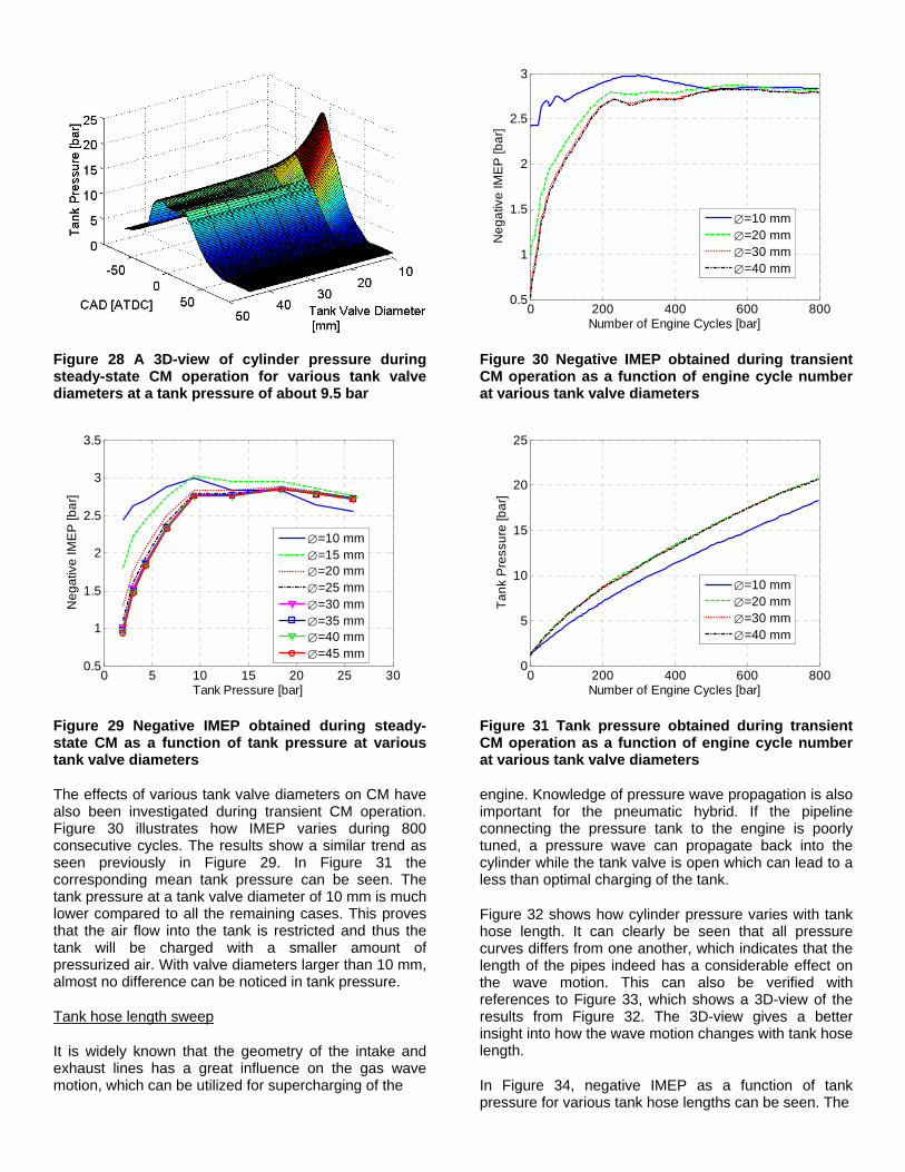
Figure 28 A 3D-view of cylinder pressure during steady-state CM operation for various tank valve diameters at a tank pressure of about 9.5 bar

Figure 29 Negative IMEP obtained during steady-state CM as a function of tank pressure at various tank valve diameters

The effects of various tank valve diameters on CM have also been investigated during transient CM operation. Figure 30 illustrates how IMEP varies during 800 consecutive cycles. The results show a similar trend as seen previously in Figure 29. In Figure 31 the corresponding mean tank pressure can be seen. The tank pressure at a tank valve diameter of 10 mm is much lower compared to all the remaining cases. This proves that the air flow into the tank is restricted and thus the tank will be charged with a smaller amount of pressurized air. With valve diameters larger than 10 mm, almost no difference can be noticed in tank pressure.

Tank hose length sweep

It is widely known that the geometry of the intake and exhaust lines has a great influence on the gas wave motion, which can be utilized for supercharging of the

Figure 30 Negative IMEP obtained during transient CM operation as a function of engine cycle number at various tank valve diameters

Figure 31 Tank pressure obtained during transient CM operation as a function of engine cycle number at various tank valve diameters

engine. Knowledge of pressure wave propagation is also important for the pneumatic hybrid. If the pipeline connecting the pressure tank to the engine is poorly tuned, a pressure wave can propagate back into the cylinder while the tank valve is open which can lead to a less than optimal charging of the tank.

Figure 32 shows how cylinder pressure varies with tank hose length. It can clearly be seen that all pressure curves differs from one another, which indicates that the length of the pipes indeed has a considerable effect on the wave motion. This can also be verified with references to Figure 33, which shows a 3D-view of the results from Figure 32. The 3D-view gives a better insight into how the wave motion changes with tank hose length.

In Figure 34, negative IMEP as a function of tank pressure for various tank hose lengths can be seen. The

0 5 10 15 20 25 300.5

1

1.5

2

2.5

3

3.5

Tank Pressure [bar]

Neg

ativ

e IM

EP

[bar

]

∅=10 mm∅=15 mm∅=20 mm∅=25 mm∅=30 mm∅=35 mm∅=40 mm∅=45 mm

0 200 400 600 8000.5

1

1.5

2

2.5

3

Number of Engine Cycles [bar]

Neg

ativ

e IM

EP

[bar

]

∅=10 mm∅=20 mm∅=30 mm∅=40 mm

0 200 400 600 8000

5

10

15

20

25

Number of Engine Cycles [bar]

Tank

Pre

ssur

e [b

ar]

∅=10 mm∅=20 mm∅=30 mm∅=40 mm

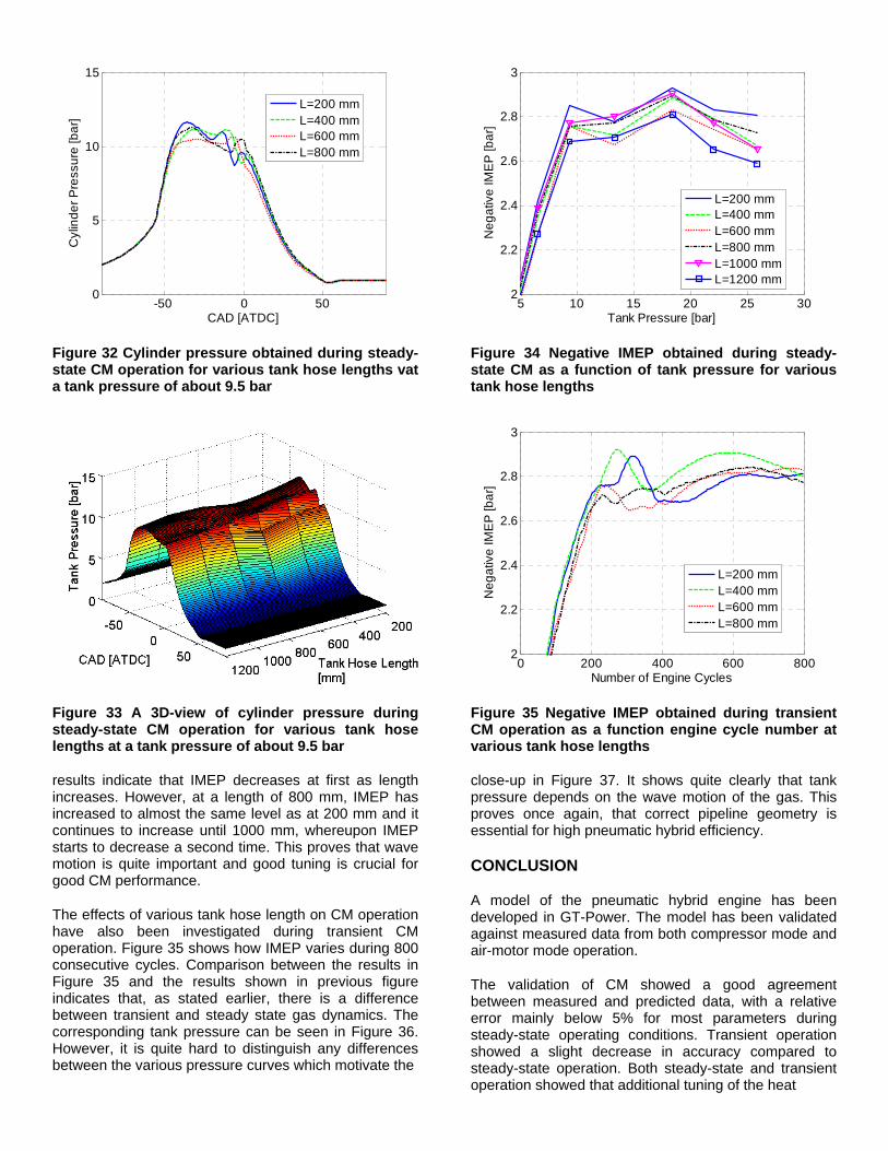
Figure 32 Cylinder pressure obtained during steady-state CM operation for various tank hose lengths vat a tank pressure of about 9.5 bar

Figure 33 A 3D-view of cylinder pressure during steady-state CM operation for various tank hose lengths at a tank pressure of about 9.5 bar

results indicate that IMEP decreases at first as length increases. However, at a length of 800 mm, IMEP has increased to almost the same level as at 200 mm and it continues to increase until 1000 mm, whereupon IMEP starts to decrease a second time. This proves that wave motion is quite important and good tuning is crucial for good CM performance.

The effects of various tank hose length on CM operation have also been investigated during transient CM operation. Figure 35 shows how IMEP varies during 800 consecutive cycles. Comparison between the results in Figure 35 and the results shown in previous figure indicates that, as stated earlier, there is a difference between transient and steady state gas dynamics. The corresponding tank pressure can be seen in Figure 36. However, it is quite hard to distinguish any differences between the various pressure curves which motivate the

Figure 34 Negative IMEP obtained during steady-state CM as a function of tank pressure for various tank hose lengths

Figure 35 Negative IMEP obtained during transient CM operation as a function engine cycle number at various tank hose lengths

close-up in Figure 37. It shows quite clearly that tank pressure depends on the wave motion of the gas. This proves once again, that correct pipeline geometry is essential for high pneumatic hybrid efficiency.

CONCLUSION

A model of the pneumatic hybrid engine has been developed in GT-Power. The model has been validated against measured data from both compressor mode and air-motor mode operation.

The validation of CM showed a good agreement between measured and predicted data, with a relative error mainly below 5% for most parameters during steady-state operating conditions. Transient operation showed a slight decrease in accuracy compared to steady-state operation. Both steady-state and transient operation showed that additional tuning of the heat

-50 0 500

5

10

15

CAD [ATDC]

Cyl

inde

r Pre

ssur

e [b

ar]

L=200 mmL=400 mmL=600 mmL=800 mm

5 10 15 20 25 302

2.2

2.4

2.6

2.8

3

Tank Pressure [bar]

Neg

ativ

e IM

EP

[bar

]

L=200 mmL=400 mmL=600 mmL=800 mmL=1000 mmL=1200 mm

0 200 400 600 8002

2.2

2.4

2.6

2.8

3

Number of Engine Cycles

Neg

ativ

e IM

EP

[bar

]

L=200 mmL=400 mmL=600 mmL=800 mm

Figure 36 Tank pressure obtained during transient CM operation as a function engine cycle number at various tank hose lengths

Figure 37 Close-up of the tank pressure curves shown in Figure 36

transfer needs to be done in order to further increase the accuracy.

The agreement between predicted and measured data for AM operation was not as good as with CM operation. The uncertainty during transient operation exceeded 40% in some cases. One reason is inadequate tuning of parameters associated with heat transfer and initial wall temperatures. Another reason is that the simulated valve lift profiles did not match the corresponding measured valve lift profiles.

A parametric study was conducted, where the influence of tank valve timing, tank valve diameter and tank hose length on pneumatic hybrid performance were investigated.

The investigation of tank valve timing illustrated the effect of tank valve opening on IMEP and torque. An engine torque of 400 Nm (2-stroke) for a 2-litre cylinder was achieved at a tank pressure of 12 bar.

The search for optimal tank valve diameter showed that as long as the valve diameter is above a threshold value, in this case 20 mm, the change in CM efficiency will be modest.

It was shown that tank hose length to a great extent influences the wave motion of the gas, and therefore a great care in choosing the right pipeline geometry is essential for good pneumatic hybrid performance.

REFERENCES

1. S. Trajkovic, P. Tunestål and B. Johansson, “Introductory Study of Variable Valve Actuation for Pneumatic Hybridization”, SAE Paper 2007-01-0288, 2007

2. S. Trajkovic, P. Tunestål and B. Johansson, “Investigation of Different Valve Geometries and Valve Timing Strategies and their Effect on Regenerative Efficiency for a Pneumatic Hybrid with Variable Valve Actuation”, SAE Paper 2008-01-1715, 2008

3. C. Thai, T-C. Tsao, M. Levin, G. Barta and M. Schechter, “Using Camless Valvetrain for Air Hybrid Optimization”, SAE Paper 2003-01-0038, 2003

4. M. Schechter, “Regenerative Compression Braking – A low Cost Alternative to Electric Hybrids”, SAE Paper 2000-01-1025, 2000

5. M. Schechter, “New Cycles for Automobile Engines”,

SAE paper 1999-01-0623, 1999 6. P. Higelin, A. Charlet, Y. Chamaillard,

"Thermodynamic Simulation of a Hybrid Pneumatic-Combustion Engine Concept International Journal of Applied Thermodynamics", Vol 5, No. 1, pp 1 – 11, ISSN 1301 9724, 2002

7. S. Trajkovic, A. Milosavljevic, P. Tunestål and B. Johansson, “FPGA Controlled Pneumatic Variable Valve Actuation”, SAE Paper 2006-01-0041, 2006

8. M. Andersson, B. Johansson and A. Hultqvist, “An Air Hybrid for High Power Absorption and Discharge”, SAE paper 2005-01-2137, 2005

9. C. Morrissey and T. Shedd, “Experimental Validation of a Carburetor Model in One-Dimensional Engine Software”, SAE Paper 2008-32-0043, 2008

10. F. Westin and H.E Ångström, “Simulation of a Turbocharged SI-Engine with Two Software and Comparison with Measured Data”, SAE Paper 2003-01-3124, 2003

0 200 400 600 8000

5

10

15

20

25

Number of Engine Cycles

Tank

Pre

ssur

e [b

ar]

L=200 mmL=400 mmL=600 mmL=800 mm

650 660 670 680 690 70018

18.5

19

19.5

Number of Engine Cycles

Tank

Pre

ssur

e [b

ar]

L=200 mmL=400 mmL=600 mmL=800 mm

11. T.T Tsung and L.L. Han, “Evaluation of dynamic performance of pressure sensors using a pressure square-like wave generator”, Measurement Science and Technology 15, pp 1133-1139, 2004

12. Scania, “Scania launches new 16-litre V8 with outstanding performance”. Available at http://www.scania.com/news/events/archive/2000/v8/press_16033.asp, (October 9, 2008)

CONTACT

Sasa Trajkovic, PhD student, Msc M. E.

E-mail: Sasa.Trajkovic@energy.lth.se

Phone: +46763161804

DEFINITIONS, ACRONYMS, ABBREVIATIONS

AM: Air-motor Mode

ATDC: After Top Dead Centre

BDC: Bottom Dead Centre

BTDC: Before Top Dead Centre

CAD: Crank Angle Degree

CM: Compressor Mode

GTP: GT-Power

ICE: Internal Combustion Engines

IMEP: Indicated Mean Effective Pressure

IVC: Inlet Valve Closing

IVO: Inlet Valve Opening

TankVO: Tank Valve Opening

TankVC: Tank Valve Closing

TDC: Top Dead Centre

RPM: Revolutions Per Minute

VVT: Variable Valve Timing