SIMULATION METHODS

IN CONFIGURATIONAL THERMODYNAMICS

Rafał Kozubski

Institute of Physics

Jagellonian University

Krakow, Poland

•MONTE CARLO

•Molecular Dynamics

•Phase Field Method

Monte Carlo methods are a widely used class of computational algorithms for simulating the behavior of various physical and mathematical systems. They are distinguished from other simulation methods (such as molecular dynamics) by being stochastic, that is nondeterministic in some manner - usually by using random numbers(or more often pseudo-random numbers) - as opposed to deterministic algorithms. Because of the repetition of algorithms and the large number of calculations involved, Monte Carlo is a method suited to calculation using a computer, utilizing many techniques of computer simulation.

Statistical Physics dealing with macroscopic systems often composed of a number of components comparable to Avogadro’s number appeared an important beneficient of new computer facilities.

A macrosystem may be found in one of its macroscopic states determined by particular microscopic states of all the components and classically represented by points in a 6N-dimensional phase space (N is the number of system components).

The macroscopic states characterised by macroscopic parameters(observables A) such as energy, volume, degree of chemical order, magnetisation etc. are usually highly degenerate with respect to the microscopic ones {}. The values of observables A measured in particular conditions (temperature, pressure, external field etc.) are identified with corresponding averages <A> over all microscopic states {} in which the system may be found in this conditions.

The central problem of statistical physics (statistical thermodynamics) is a calculation of the values of <A>. The averaging is performed over an appropriate ensemble of macroscopic systems representing the related microscopic states. An ensemble is characterised by so called density () defined in the way that

is a probability that a system in the ensemble is in the microscopic state (see e.g. Huang, 1963).The principle achievement of the founders of statistical physics was the derivation of formulae for the densities eq() corresponding to ensembles of systems in equilibrium state.

Complete description of the system thermodynamics is derivable from the sum

called a partition function

P

eqZ

Type of ensemble Usage Density function eq,

H denotes Hamiltonian of

the system

Microcanonical ensemble Isolated systems with

fixed energy E

Canonical ensemble Systems with fixed volume

V and number of particles

N studied at fixed

temperature T determined

by thermal bath

Isothermal-Isobaric

ensemble

Systems with fixed

number of particles N

studied at fixed pressure P

and temperature T

determined by thermal

bath

Grand Canonical

ensemble

Opened systems with

fixed volume V studied at

fixed temperature T

determined by thermal

bath and fixed chemical

potentials k k – chemical potential

EH i ,

Tk

PVH

B

iexp

Tk

H

B

iexp

Tk

NH

B

k

kiki

exp

SAMPLING

If A() denotes the value of the observable A in the microscopic state then:

AZ

APA1

where the sum covers all possible microscopic states (whose number is most often extremely large or even infinite) and its strict calculation is usually unfeasible. The basic idea is to approximate the complete sum () by a partial one performed over some subset {i, i = 1, …, M} of the microscopic states

M

kk

M

iii A

A

1

1

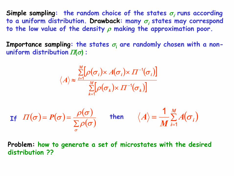
Simple sampling: the random choice of the states i runs according to a uniform distribution. Drawback: many i states may correspond to the low value of the density making the approximation poor.

Importance sampling: the states i are randomly chosen with a non-uniform distribution () :

M

kkk

M

iiii A

A

1

1

1

1

P

M

iiA

MA

1

1If then

Problem: how to generate a set of microstates with the desireddistribution ??

Markov chains as a tool for importance sampling

111111,;.......,, nnnnntytytyP

Probability that an event yn occurs at a time tn in condition that events y1, y2,...occured at times t1, t2,...

Markov chain of events:

1111111111,,,;.......,,

nnnnnnnnntytyPtytytyP

If states of the systems in an ensemble change due to Markov processes, the time evolution of the probability distribution P()is given by a Master equation:

j

jijij

jii PWPW

dt

dP

The evolution leads to a stationary distribution Pst():

0dt

dP ist

provided that:

j

jstijistj

ji PWPW

hence:

ieq

jeq

ieq

jeq

ij

ji

P

P

W

W

Detailed balace conditionfor transition frequencies W

The detailed balance guarantees a convergence of a Markov chain to Peq().

tW

ji

ji

Transition probability per time

Simulation of Markov chains is a typical task realised by means of Monte Carlo algorithms:

Stochastics is digitally simulated by random number generators –i.e. computer codes generating with a uniform probability numbers from a fixed interval (most often 0,1).

Basic idea:

Let a certain event occur in reality with a probability P

Random number R 0,1 is generated

The event occurs in Monte Carlo simulation if R 0,P

The Monte Carlo method may be basically applied to diverse kinds of problems in statistical physics:

Simulation and characterisation of system properties in thermodynamic equilibrium:

The procedure starts from a system in some (arbitrary) initial state. Subsequently, an evolution of the system is simulated as a Markov chain of microscopic states i with the transition frequencies W(ij) obeying detailed balance corresponding to the particular conditions of the equilibrium state in question. The applied algorithm must enable to follow the evolution of some macroscopic parameter of the system (for example its energy), so that it is possible to observe the approach of equilibrium (microscopic states are in dynamical equilibrium with the distribution Peq() ). Once this stage is attained, the microscopic states i of the system appearing at particular time moments may be randomly sampled and used in the averaging procedure(effectively, time averaging is done).

Example:

STUF

M

iiE

MU

1

1

i

iiB PPkS ln

P(i) is the probability for the occurrence of the microstate i.

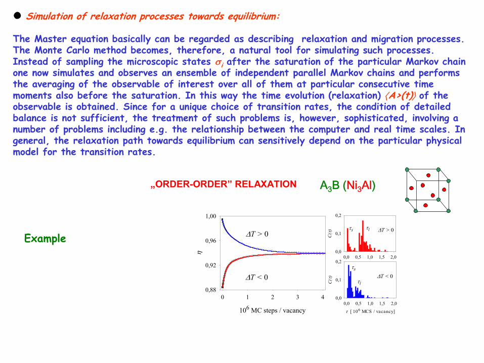
Simulation of relaxation processes towards equilibrium:

The Master equation basically can be regarded as describing relaxation and migration processes. The Monte Carlo method becomes, therefore, a natural tool for simulating such processes. Instead of sampling the microscopic states i after the saturation of the particular Markov chain one now simulates and observes an ensemble of independent parallel Markov chains and performs the averaging of the observable of interest over all of them at particular consecutive time moments also before the saturation. In this way the time evolution (relaxation) A>(t) of the observable is obtained. Since for a unique choice of transition rates, the condition of detailed balance is not sufficient, the treatment of such problems is, however, sophisticated, involving a number of problems including e.g. the relationship between the computer and real time scales. In general, the relaxation path towards equilibrium can sensitively depend on the particular physical model for the transition rates.

0.0 0.5 1.0 1.5 2.0

C()

0.0

0.1

0.2

s l T > 0

[ 106 MCS / vacancy]

0.0 0.5 1.0 1.5 2.0

C()

0.0

0.1

0.2

s

l

T < 0

106 MC steps / vacancy

0 1 2 3 4

0.88

0.92

0.96

1.00

T > 0

T < 0

0,0 0,5 1,0 1,5 2,0

C()

0,0

0,1

0,2

s l T > 0

[ 106 MCS / vacancy]

0,0 0,5 1,0 1,5 2,0

C()

0,0

0,1

0,2

s

l

T < 0

106 MC steps / vacancy

0 1 2 3 4

0,88

0,92

0,96

1,00

T > 0

T < 0

„ORDER-ORDER” RELAXATION A3B (Ni3Al)

Example

Simulation of non-equilibrium processes and transport phenomena

Such processes, as consisting of effective transitions between microscopic states constitute a natural object for studies by means of MC methods. Non equilibrium character of the phenomenon means that detailed balance must no longer be obeyed by the transition frequencies which are to model particular microscopic reactions involved in the process.

Examples:

Crystal growth according to the Kossel model. In this model three atomistic-scale processes: deposition, evaporation and diffusion compete. Particular frequency (rate) is modelled and attributed to each process and its selective influence on the overall effect (e.g. crystal growth rate) may then be studied by means of MC.

Transport phenomena may be studied by means of MC both in stationary and non-stationary states of the systems simply by monitoring the process of transport during the simulated Markov chain. The standard method consists of monitoring mean-squared displacement R2

A(V)(t) of a tracer atom (A)/vacancy (V) as a function of MC time.

Vacancy/tracer diffusion constant DV(A):

AVAV

AVt

AV tRtN

D2

6

1lim

A

AA

Ana

nRf

2

2

Correlation factor for atoms A

Limitations:

Thermodynamic laws correspond in statistical physics to the thermodynamic limitN , where N denotes the number of particles in the system. It is obvious that when numerically simulating a system, one always operates with a finite value of N.

The “simplest” task aiming in the elimination of the parasitic influence of the sample limits on the simulated effects is usually realised by the application of periodic boundary conditions consisting of the consideration of the opposite sample boundaries as neighbouring parts. The well-known two-dimensional analogue of this idea is a transformation of a plane into a torus.

Despite compensating the boundary (surface) effects, periodic boundary conditions cannot remove the finite-size-caused limitation in the consideration of any distance-dependencies. This applies e.g. to correlation lengths (which cannot exceed the sample size) and results in characteristic blunting (rounding) of singularities marking continuous and discontinuous phase transitions.

\\

Numerical implementation of MC

(choice of transition frequencies W(i j))

Classical approach(Metropolis, N., Rosenbluth, A.W., Rosenbluth, N.N., Teller, A.H., and Teller, E. (1953),

J.Chem.Phys. 21, 1087)

Tk

E

E

ETk

E

WB

B

ji

exp,min

0,

0,exp

11

1

1

E=Efin – Eini, system energy equals Eini in the microstate i and Efin in the microstate j;kB and T denote the Boltzmann constant and temperature, respectively and is a time scale constant

Although the Metropolis transition frequencies obviously fulfil the detailed balance their use may be disadvantageous at high temperatures, where due to the transition probabilities approaching the value of 1, the system being off equilibrium keeps oscillating between different microscopicstates, which makes the simulated process not perfectly ergodic.

Glauber algorithm: (Glauber, R.J., (1963), J.Math.Phys. 4, 294)

Tk

E

Tk

E

Tk

E

Tk

E

Tk

E

W

B

B

B

fin

B

ini

B

fin

ji

exp1

exp

expexp

exp11

1,

2

1

ji

ji

WE

TW

Probabilistic rationale:The probability of an event: “the system either transforms from i to j or remains in i” is in this particular case equal to 1. On the other hand, it must be equal to a sum of the two corresponding probabilities.

The simulation algorithms involving the above formulae for W(ij) work usually in the following cycles:

The system is in some microscopic state I

Another microscopic state ji is chosen at random from theset {i}

Transition ij is executed or suppressed according to theprobability W(ij)

Time is incremented by

Drawback:

A number of MC steps are „lost” – no transition is executed

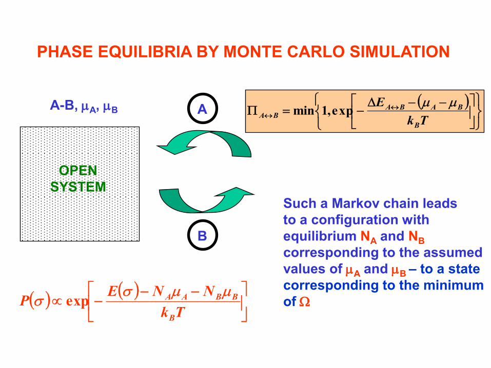
PHASE EQUILIBRIA BY MONTE CARLO SIMULATION

A-B, A, B

Tk

NNEP

B

BBAA exp

OPEN

SYSTEM

A

B

Tk

E

B

BABABA

exp,1min

Such a Markov chain leads

to a configuration with

equilibrium NA and NB

corresponding to the assumed

values of A and B – to a state

corresponding to the minimum

of W

20 40 60

-100000

0

100000

200000

300000

400000

500000

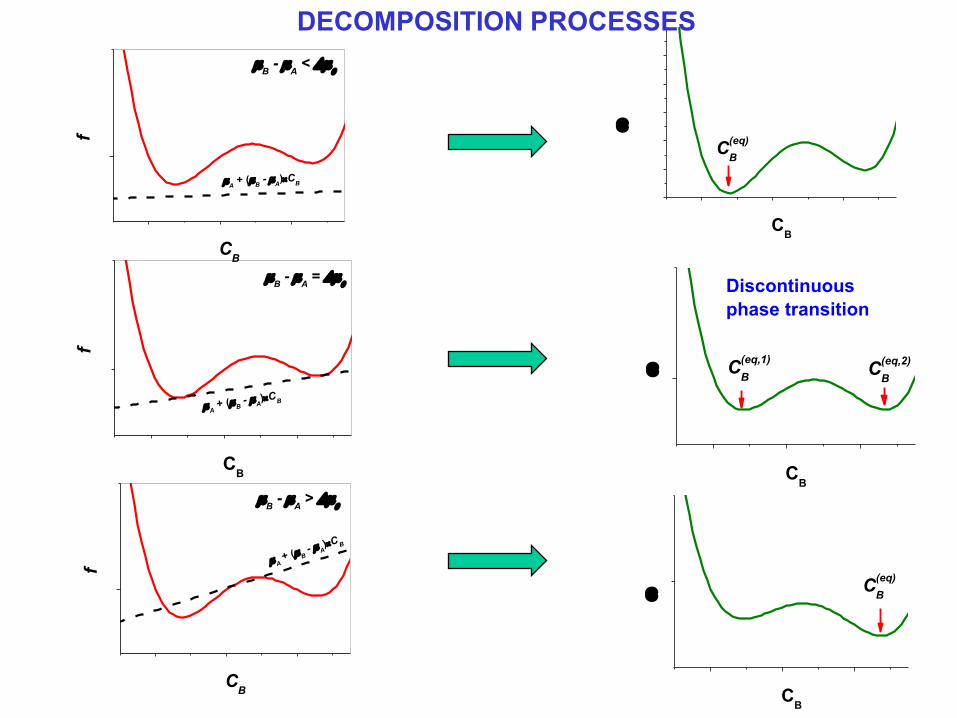
CB

C(eq)

B

20 40 60

0C

(eq,1)

B

CB

C(eq,2)

B

Discontinuous

phase transition

20 40 60

0

CB

C(eq)

B

20 40 60

0

f

CB

A + (B

- A)CB

B -

A =

20 40 60

0

B -

A <

A + (

B -

A)C

B

f

CB

20 40 60

0

B -

A >

A + (B

- A)C B

f

CB

DECOMPOSITION PROCESSES

eV

VC

Two phase coexistence region

Crystal with

equilibrium vacancy

concentration

Jaggelonian University DIMAT 2008

APPLICATION:

LONG-RANGE ORDERING

IN INTERMETALLICS

„Order-disorder” phase transformations

Continuous (2nd-order)

transformation

Discontinuous

(1st-order)

transformation

MONTE CARLO SIMULATIONS:

•A3B or AB binary system with L12, L10 or B2 superstructure,

•40 40 40 cubic cells,

•1 vacancy (10 vacancies in a piloting study)

general assumption: vacancy mechanism of atomic migration

Distance

-2 0 2 4 6 8

En

erg

y o

f a

sy

ste

m

-2

-1

0

1

2

3

Ei

j

E+

kT

E

kT

E

w ji

exp1

exp1

Glauber dynamics algorithm:

„Residence-time“ algorithm:

kT

EEw iii exp0

0

1

0 ,exp

tkT

EE

l

ll

Kinetic Monte CarloKMC

SUPERSTRUCTURE STABILITY

Tred

0,85 0,90 0,95 1,00 1,05 1,10 1,15

eq

-0,2

0,0

0,2

0,4

0,6

0,8

1,0

L10

L12

B2

L12 L10 B2

DO

redT

TT

APPLICATION:

PHASE EQUILIBRIA

Vacancy concentration in

intermetallics

MODEL: EQUILIBRIUM CONCENTRATION OF THERMAL VACANCIES

IN LONG-RANGE ORDERED SYSTEMS

Ising lattice gas:

NA A-atoms, NB B-atoms, NV vacancies

NA + NB + NV = N = const

W = 2VAB-VAA-VBB < 0

(tendency for ordering)

VVV = 0

W. Schapink, Scr. Metall. 3, 113, (1969).

S. H. Lim, G. E. Murch, W. A. Oates, J. Phys. Chem. Solids 53, 181, (1992)

R. Kozubski, Acta Metall. Mater. 41, 2565, (1993).

The model is solved by means of two methods:

•Bragg-Williams approximation (mean field)A.Biborski, L.Zosiak, R. Kozubski, V. Pierron-Bohnes, Intermetallics, 17, 46-55, (2009).

•Semi-Grand Canonical Monte Carlo (SGCMC) simulationsA.Biborski, L.Zosiak, R. Sot, R. Kozubski, V. Pierron-Bohnes, submitted to J.Chem.Phys.

Semi-Grand Canonical MC of a ternary A-B-V lattice gas:

•Generation of a sample 15x15x15 unit cells,

periodic boundary conditons

•Determination of relative chemical potentials AV and BV

•Random choice of a lattice site

•Random choice of the exchange type:

Species Exchange type

A A A A - B A - V

B B - A B - B B - V

V V - A V - B V - V

•Execution of the exchange according to Metropolis probability:

Tk

E

B

pVqVqp

qp

exp,1min

TYPICAL RESULT IN B2

SUPERSTRUCTURE

Equilibrium

vacancy concentration

IN THE LATTICE GAS

Limits of equilibrium

vacancy concentration

IN CRYSTALS with diverse

composition (hysteresis)

Equilibrium of

vacancy-poor (crystal)

and vacancy-rich phases

T = const

CV facet

CA/CB = const path

Hysteresis

and thermodynamic integration result

Fig.5. Sections of the miscibility gap of the A-B-V lattice gas. Vacancy-

poor borders of the sections correspond to: (a) A0.52B0.48-V (d=0.48); (b)

A0.5B0.5-V (d=0.5); (c) A0.48B0.52-V