simulation der partikeldynamik mittels der diskrete ...€¦ · 1 simulation der partikeldynamik...
TRANSCRIPT
1
Simulation der Partikeldynamik mittels der Diskrete Elemente Methode:
Einführung in PFC Programmversionen
Particle Flow Code in 2 Dimensions (PFC2D, Version 4.0) begrenzt auf 1.000 Partikel
Particle Flow Code in 3 Dimensions (PFC3D, Version 4.0) begrenzt auf 5.000 Partikel
6 Bedienungshandbücher in Englisch Programmebenen
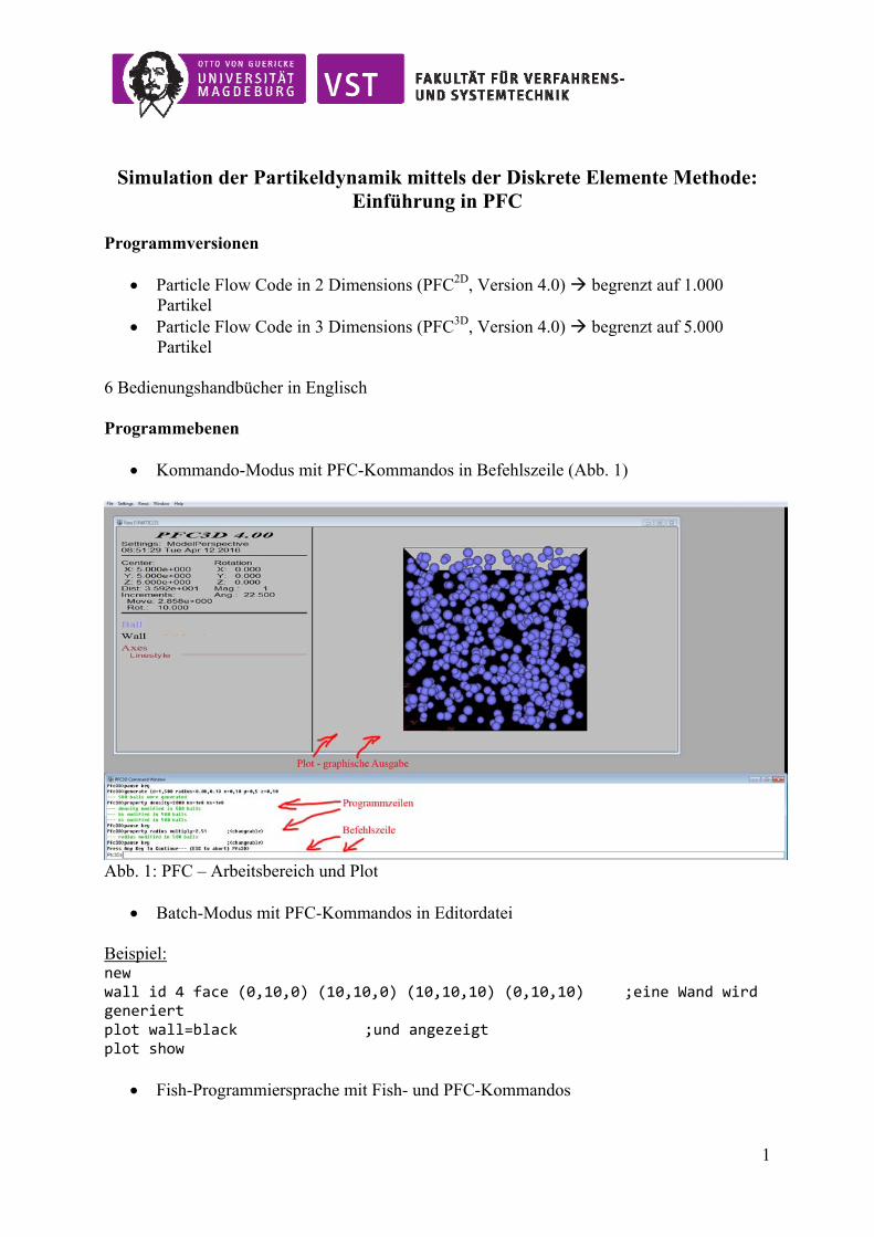
Kommando-Modus mit PFC-Kommandos in Befehlszeile (Abb. 1)
Abb. 1: PFC – Arbeitsbereich und Plot
Batch-Modus mit PFC-Kommandos in Editordatei Beispiel: new wall id 4 face (0,10,0) (10,10,0) (10,10,10) (0,10,10) ;eine Wand wird generiert plot wall=black ;und angezeigt plot show
Fish-Programmiersprache mit Fish- und PFC-Kommandos

2
Beispiel: new define make_wall_and_calculate hh=22 ;Zuweisungsoperation abc=hh*3+5 ;Rechnung command wall id 4 face (0,10,0) (10,10,0) (10,10,10) (0,10,10) ;PFC‐Kommando endcommand end make_wall_and_calculate plot wall=black plot show
C++-Programmiersprache (optional, verfügbar in Vollversion)
Nützliche Tastaturbefehle: F3 Wiederholung der letzten Eingabezeile Esc abbrechen des Programms Bei aktivem Plot: Strg + C Ploteinstellungen Richtungstasten Bewegung des Plots M heranzoomen Strg + R automatische Zentrierung des Plots mit Rotation (0,0,0) X Rotation um die x-Achse Y Rotation um die y-Achse Z Rotation um die z-Achse Verringerung der Rechenzeit: Partikelgröße keine kleinen Partikel (monodisperse Partikel) Steifigkeit keine hohen Steifigkeiten Ausschalten der Plots set pinterval xyz Plotaktualisierung (aller xyz Zeitschritte) anpassen/verringern Differential Density Scaling Erklärung weiter hinten im Dokument Grundlegende PFC-Kommandos Nützliche Befehle: ; - Semikolon Kommentar & - und Fortsetzung der auf 80 Zeichen begrenzten Eingabezeile auf der
nächsten Zeile pause key unterbricht das Programm (Any Key to continue) new leert den Speicher, damit ein neues Programm gestartet werden kann Alle Befehle weisen dieselbe Struktur auf. Sie bestehen aus einem primären Befehlswort gefolgt von einem oder mehreren Keywords und einem numerischen Input. COMMAND keyword value . . . <keyword value . . . >

3
Die Befehle können ausgeschrieben werden, die fettgedruckten Buchstaben müssen aber mindestens angegeben werden. Befehle, Keywords und numerische Werte können durch Leerzeichen, Komma(s), Runde Klammern ( ) oder ein Gleichheitszeichen = getrennt werden. Groß- und Kleinbuchstaben sind erlaubt. Beispiel: new wall id=1 kn=1e8 ks=1e8 friction=0.1 face= (0,0,0) (10,0,0) (10,10,0) (0,10,0) ;bottom wall wall id=2 kn=1e8 ks=1e8 friction=0.1 face= 0,0,0 0,10,0 0,10,10 0,0,10 ;left wall wall id=3 kn=1e8 ks=1e8 friction=0.1 face= 10 0 0 10 0 10 10 10 10 10 10 0 ;right wall wall id 4 kn 1e8 ks 1e8 friction 0.1 face 0 0 0 0 0 10 10 0 10 10 0 0 ;front wall WALL id=5 KN=1e8 KS=1e8 FRICTION=0.1 FACE= (0,10,0) (10,10,0) (10,10,10) (0,10,10) ;back wall w id=6 kn=1e8 ks=1e8 f=0.1 fa= (0,10,10) (10,10,10) (10,0,10) (0,0,10) ;upper wall pause key plot create schwarze_wand ;Plot definieren plot add wall black ;Wände zum Plot hinzufügen plot show ;Plot anzeigen
Befehlswort wall Wand Keywords id Identifikationsnummer
kn Normalsteifigkeit ks Schersteifigkeit friction Reibungskoeffizient face bei einer begrenzten (finiten) Wand folgen daraufhin die
Koordination …
Numerische Eingabewerte 1e8, 0, 10 Wand aktive Seite Korkenzieherregel / Rechte-Faust-Regel
4
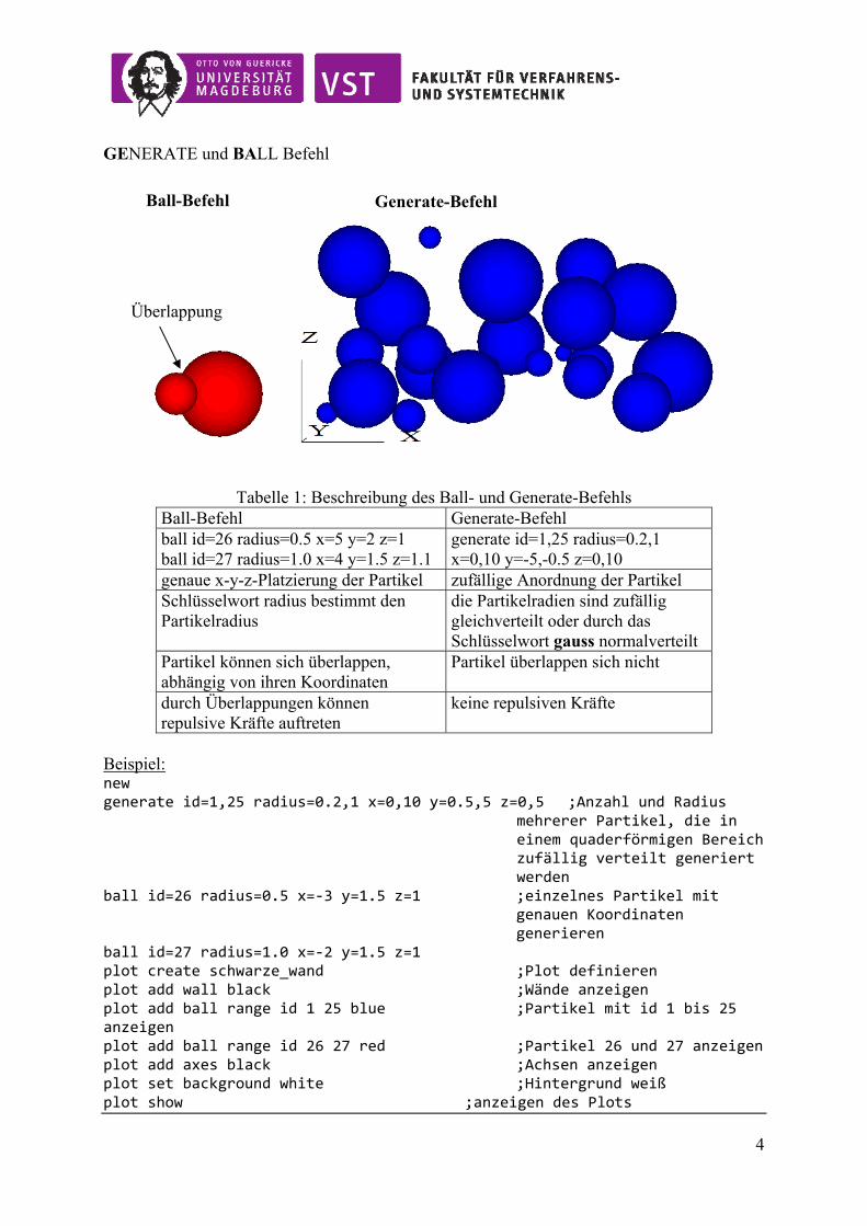
GENERATE und BALL Befehl
Tabelle 1: Beschreibung des Ball- und Generate-Befehls Ball-Befehl Generate-Befehl ball id=26 radius=0.5 x=5 y=2 z=1 ball id=27 radius=1.0 x=4 y=1.5 z=1.1
generate id=1,25 radius=0.2,1 x=0,10 y=-5,-0.5 z=0,10
genaue x-y-z-Platzierung der Partikel zufällige Anordnung der Partikel Schlüsselwort radius bestimmt den Partikelradius
die Partikelradien sind zufällig gleichverteilt oder durch das Schlüsselwort gauss normalverteilt
Partikel können sich überlappen, abhängig von ihren Koordinaten
Partikel überlappen sich nicht
durch Überlappungen können repulsive Kräfte auftreten
keine repulsiven Kräfte
Beispiel: new generate id=1,25 radius=0.2,1 x=0,10 y=0.5,5 z=0,5 ;Anzahl und Radius
mehrerer Partikel, die in einem quaderförmigen Bereich zufällig verteilt generiert werden
ball id=26 radius=0.5 x=‐3 y=1.5 z=1 ;einzelnes Partikel mit genauen Koordinaten generieren
ball id=27 radius=1.0 x=‐2 y=1.5 z=1 plot create schwarze_wand ;Plot definieren plot add wall black ;Wände anzeigen plot add ball range id 1 25 blue ;Partikel mit id 1 bis 25 anzeigen plot add ball range id 26 27 red ;Partikel 26 und 27 anzeigen plot add axes black ;Achsen anzeigen plot set background white ;Hintergrund weiß plot show ;anzeigen des Plots
Ball-Befehl Generate-Befehl
Überlappung

5
property Definition der Eigenschaften existierender Partikel change Synonym zu property initialize Synonym zu property Stoffeigenschaften für die Partikeln und ihre Verbindungen property density=2650 kn=1e8 ks=1e8 Dichte, Normal- und Schersteifigkeit property radius multiply=1.51 Vergrößerung des Radius Die Anzahl, die Koordinaten, die Radien, die Dichten und die Steifigkeiten der Partikel, die Koordinaten und die Steifigkeiten der Wände und die Erdbeschleunigung werden festgelegt. Daraus ergeben sich die wirkenden Gewichts- und Abstoßkräfte, die Beschleunigungen und Spannungen in den Überlappungen. Beispiel: new plot create schwarze_wand plot add wall black plot add ball range id 1 25 blue plot add ball range id 26 27 red plot add axes black plot set background white plot show generate id=1,25 radius=0.2,1 x=0,10 y=0.5,5 z=0,5 ball id=26 radius=0.5 x=‐3 y=1.5 z=1 ball id=27 radius=1.0 x=‐2 y=1.5 z=1 property density=2650 kn=1e8 ks=1e8 ;zählt für alle existierenden Partikel pause key range name=bälle_1_25 id=1,25 ;Definition des Bereichs der Partikel
mit id 1 bis 25 property radius multiply=1.51 range=bälle_1_25 ;Zuweisung der Vergrößerung
des Radius für den definierten Bereich
pause key set gravity=(0,0,‐9.81) ;Gravitationsbeschleunigung cycle 6000 ;Zeitschritte
Tabelle 2: Keywords in den Befehlen
programminterne Parameter
Stoffdaten wall-Befehl für Wände property-Befehl für Partikel
Randbedingungen: wall-Befehl für Wände property-Befehl für Partikel
Identifikations-nummer: ball – Partikel clump – Clump history –
Aufzeichnen von Messwerten
measure – Messkreis
wall – Wand
radius kn – Normalsteifigkeit ks – Schersteifigkeit density – Dichte friction – Reibung damping – viskose
Dämpfung Kontaktbindung n_bond – Normalsteifigkeit
x-, y-, z-Koordinaten xdisplacement, ydisplacement,
zdisplacement – x-, y-, z-Weg xvelocity, yvelocity, zvelocity –
x-, y-, z-Geschwindigkeit xspin, yspin, zspin – x-, y-, z-
Rotationsgeschwindigkeit gravity – Erdbeschleunigung xforce, yforce, zforce – x-, y-,

6
Ausgabefenster position –
Position size – Größe Farbe etc.
s_bond – Schersteifigkeit Parallelbindung pb_kn – Normalsteifigkeit pb_ks – Schersteifigkeit pb_nstrength –
Normalfestigkeit pb_sstrengt –
Scherfestigkeit pb_radius – Radius etc.
z-Kraft xmoment, ymoment, zmoment
– x-, y-, z-Drehmoment etc.
Tabelle 3: Definition der Eingabe- und Ausgabewerte
Eingabewert Länge m Dichte kg/m3 Gravitationsbeschleunigung m/s2 Steifigkeit der Wände und Partikel N/m Steifigkeit der Parallelbindung Pa/m
N/(m2m) Festigkeit von Kontaktbindungen N Festigkeit von Parallelbindungen N/m2
Ausgabewert Kraft N Spannung Pa
Zerlegung der Kontaktkraft in eine Normal- und eine Scherkomponente F – Kontaktkraft Fn – Normalkraft kn – Normalsteifigkeit Fs – Scherkraft ks – Schersteifigkeit
FFn
Fs
kn
ks
F
Kontaktfläche
kn
7
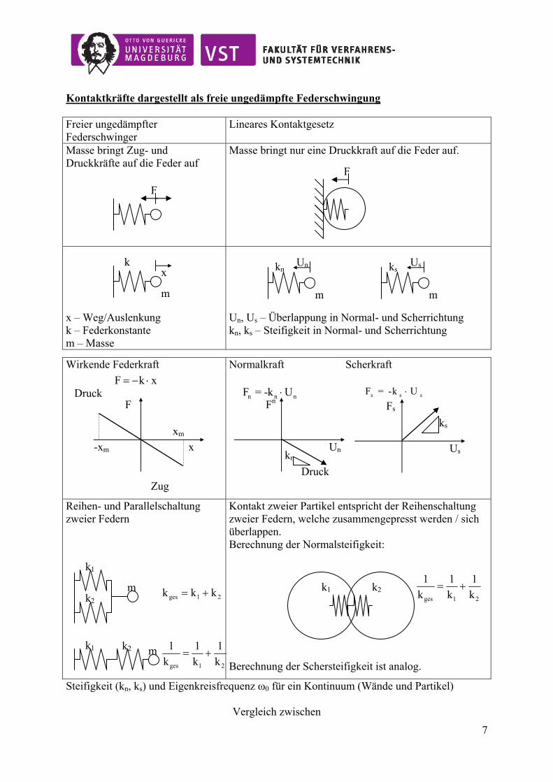
Kontaktkräfte dargestellt als freie ungedämpfte Federschwingung Freier ungedämpfter Federschwinger
Lineares Kontaktgesetz
Masse bringt Zug- und Druckkräfte auf die Feder auf
Masse bringt nur eine Druckkraft auf die Feder auf.
x – Weg/Auslenkung k – Federkonstante m – Masse
Un, Us – Überlappung in Normal- und Scherrichtung kn, ks – Steifigkeit in Normal- und Scherrichtung
Steifigkeit (kn, ks) und Eigenkreisfrequenz ω0 für ein Kontinuum (Wände und Partikel)
Vergleich zwischen
Wirkende Federkraft
Normalkraft Scherkraft
Reihen- und Parallelschaltung zweier Federn
Kontakt zweier Partikel entspricht der Reihenschaltung zweier Federn, welche zusammengepresst werden / sich überlappen. Berechnung der Normalsteifigkeit: Berechnung der Schersteifigkeit ist analog.
xk
m
Us ks
m m
kn Un
F
F
21ges kkk
21ges k
1
k
1
k
1
xkF n n nF = -k U
21ges k
1
k
1
k
1k1 k2
x
F
xm
-xm
Druck Zug
Druck
Un
Fn
kn
s s sF = -k U
Us
Fs
ks
k1
k2
m
k1 k2 m

8
mechanischem Schwinger schwingendem Kontinuum
Federschwinger Stabschwinger Auslenkung: x(t)
Auslenkung:
0
0100 l
l)t(ll)t(l)t(l
- Dehnung Hookesches Gesetz für Federschwinger:
FF = -kx
FF - Federkraft k - Federkonstante x - Weg
Hookesches Gesetz für das Kontinuum
0l
lEE
0S 0
0
EAF = -E A ε = - Δl
l
E - Elastizitätsmodul A0 - Querschnittsfläche l0 - Ausgangslänge
Federsteifigkeit: 20k = m ω
Kontinuum Steifigkeit: 200
0
EAk = = m ω
l
Trägheitskraft: TF = ma = mx Trägheitskraft: T 0F = mx = m Δl = ml ε
Bewegungsgleichung:
T FF = F
mx = -kx k
x + x = 0m
Bewegungsgleichung:
T SF = F
0 0ml ε = -EA ε
0
0
EAε + ε = 0
ml
Eigenkreisfrequenz:
0 0
kω = 2πf =
m
Eigenkreisfrequenz:
0
00 ml
EA
FF
FT
m
x(t)
m
k
Ruhelage Auslenkung
m
Ruhelage
lo(t)
FT
FS
m
A0 E
lo
Auslenkung
l1
9
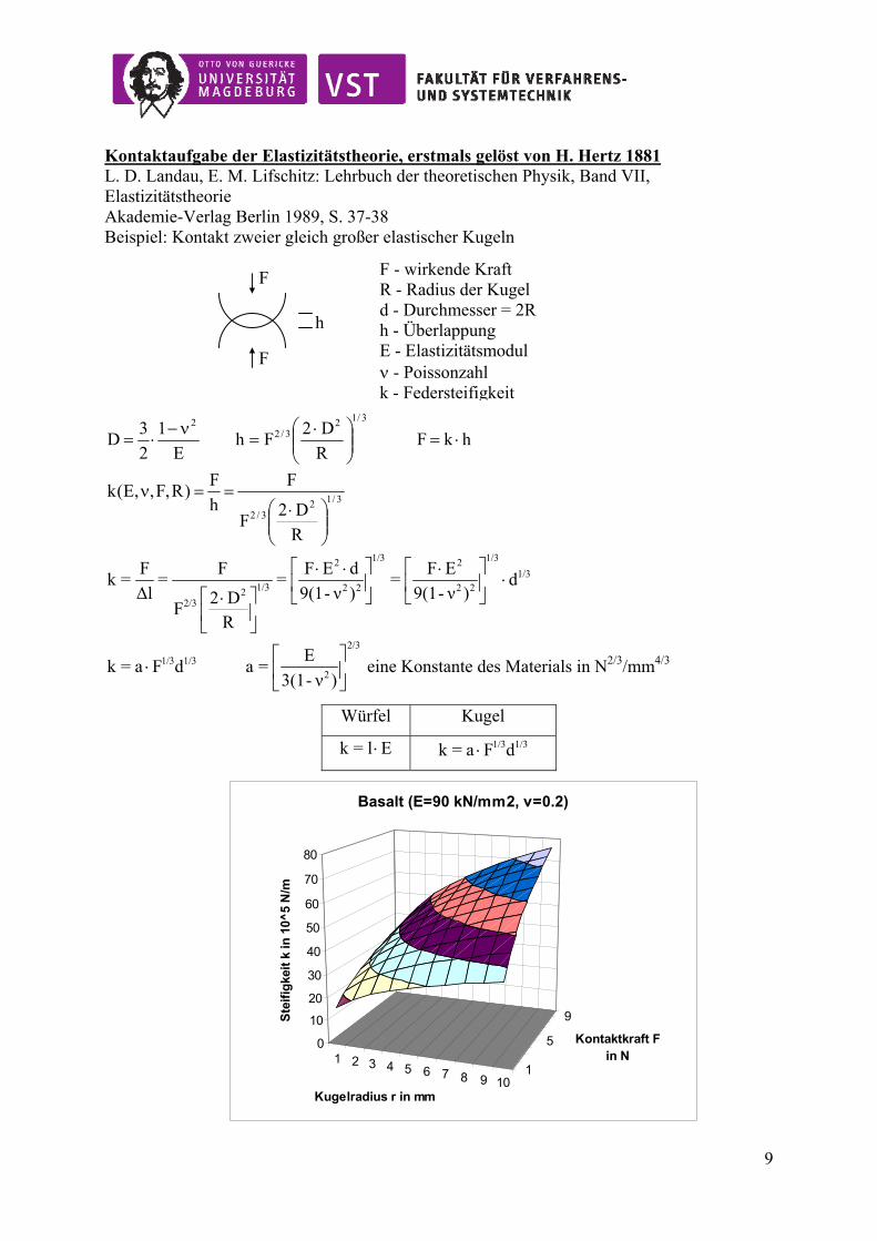
Kontaktaufgabe der Elastizitätstheorie, erstmals gelöst von H. Hertz 1881 L. D. Landau, E. M. Lifschitz: Lehrbuch der theoretischen Physik, Band VII, Elastizitätstheorie Akademie-Verlag Berlin 1989, S. 37-38 Beispiel: Kontakt zweier gleich großer elastischer Kugeln
E
1
2
3D
2
3/123/2
R
D2Fh
hkF
3/123/2
R
D2F
F
h
F)R,F,,E(k
1/3 1/32 21/3
1/3 2 2 2 222/3
F F F E d F Ek = = = = d
Δl 9(1- ν ) 9(1- ν )2 DF
R
1/3 1/3k = a F d 2/3
2
Ea =
3(1- ν )
eine Konstante des Materials in N2/3/mm4/3
Würfel Kugel
k = l E 1/3 1/3k = a F d
h
F
F
F - wirkende Kraft R - Radius der Kugel d - Durchmesser = 2R h - Überlappung E - Elastizitätsmodul - Poissonzahl k - Federsteifigkeit
1 2 3 4 5 6 7 8 9 101
5
9
0
10
20
30
40
50
60
70
80
Ste
ifig
keit
k in
10^
5 N
/m
Kugelradius r in mm
Kontaktkraft F in N
Basalt (E=90 kN/mm2, v=0.2)

10
Federsteifigkeit zweier gleicher elastischer Kugeln nach Hertz (1881) in Abhängigk. von Material, Kontaktfläche und -kraft (Würfel im Vergleich)
1e+02
1e+03
1e+04
1e+05
1e+06
1e+07
1e+08
1e+09
0,001 0,01 0,1 1 10 100 1000
Kugeldurchmesser/Würfelkantenlänge in mm
Fe
de
rste
ifig
ke
it in
N/m
Silikonkautschuk F=1mN
Polystyrol F=1mN
Kalkstein/Quarz F=1mN
Basalt F=1mN
Baustahl F=1mN
Silikonkautschuk F=1N
Polystyrol F=1N
Kalkstein/Quarz F=1N
Basalt F=1N
Baustahl F=1N
Silikonkautschuk F=1kN
Polystyrol F=1kN
Kalkstein/Quarz F=1kN
Basalt F=1kN
Baustahl F=1kN
Würfel-Silikonkautschuk
Würfel-Polystyrol
Würfel-Kalkstein/Quarz
Würfel-Basalt
Würfel-Baustahl

11
Berechnung in Zeitschritten
Kraft-Weg-Gesetzangewendet auf Kontakte
Bewegungsgesetzangewendet auf Partikel
nnn UkF sss UkF
ii xmF ii JM
geradlinige Bewegung:Rotationsbewegung:i..2 für 2D i..3 für 3D
Normalkraft:Scherkraft :U.. Überlappung
Kontaktkräfte
Positionskorrektur von Partikeln, Wänden und Kontakten
Randbedingungengesetzt durch Wände/Partikel
- einwirkende Kräfte - fixierte Positionen und Geschw.
Einsatz der Software PFC3D der Fa. Itasca Co., Minnesota US
12
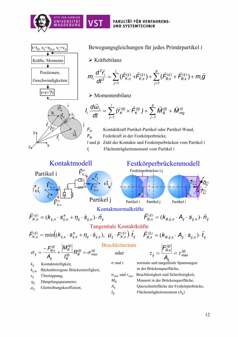
Bewegungsgleichungen für jedes Primärpartikel i
Kräftebilanz
FK Kontaktkraft Partikel-Partikel oder Partikel-Wand,
FB Federkraft in der Festkörperbrücke,
l und p Zahl der Kontakte und Festkörperbrücken vom Partikel i
Ii Flächenträgheitsmoment vom Partikel i
Momentenbilanz
(i)mg
p
1j
(ij)B
1j
(ij)K
(ij)K
ii MM)Fr(dt
ωdI
l
Kräfte, Momente
Positionen,
Geschwindigkeiten
t=t+?t
t=t0, xi=x0,i, vi=v0
gmFFFFdt
rdm i
ijsB
p
j
ijnB
ijsK
j
ijnK
ii
)()( )(,
1
)(,
)(,
1
)(,2
2 l
Festkörperbrückenmodell
Kontaktnormalkräfte
ijnijijanijnij
ijnK nsηskF
)( ,,,)(
,
ijijnKijsijij
asijsij
ijsK tFμsηskF
)(
,,,,)(
, ),(min
Tangentiale Kontaktkräfte
ijnijijnijBijnB nsAkF
)( ,,,
)(,
ijsijijsijBijsB tsAkF
)( ,,,
)(,
kij Kontaktsteifigkeit,
kij,B flächenbezogene Brückensteifigkeit,
sij Überlappung,
ij Dämpfungsparameter,
ij Gleitreibungskoeffizient,
(ij)max
(ij)B(ij)
B
(ij)B
ij
(ij)nB,
ij RI
M
A
F
(ij)
maxij
(ij)sB,
ij A
F oder
Bruchkriterium
und normale und tangentiale Spannungen
in der Brückenquerfläche,
max und max Bruchfestigkeit und Scherfestigkeit,
MB Moment in der Brückenquerfläche,
Aij Querschnittsfläche der Festkörperbrücke,
IB Flächenträgheitsmoment (Aij)
Kontaktmodell
13
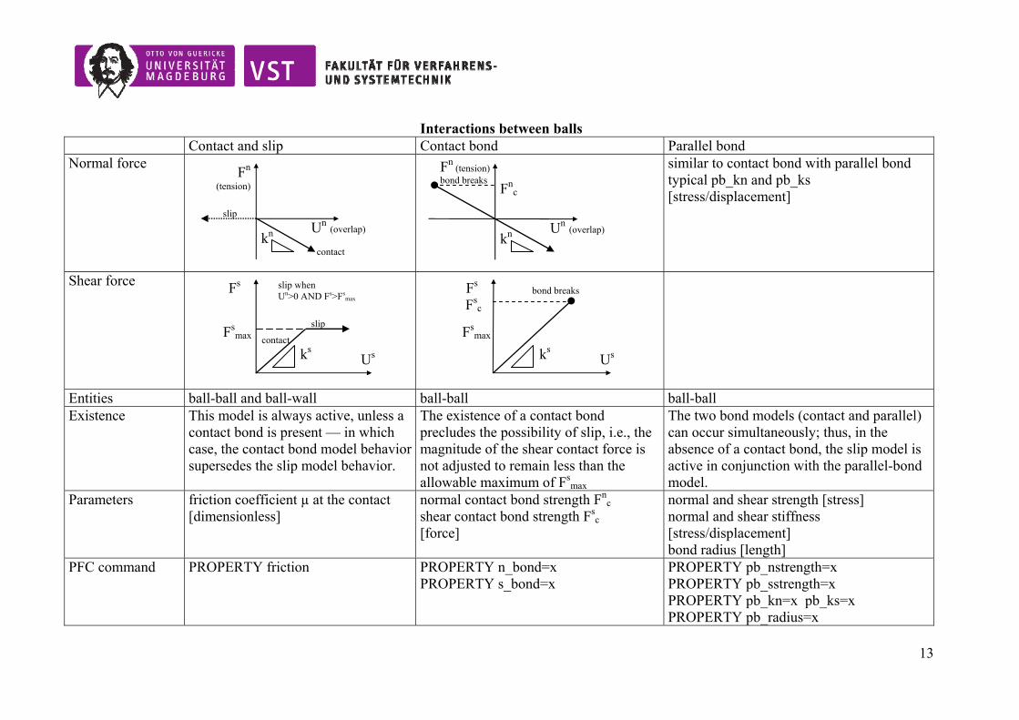
Interactions between balls Contact and slip Contact bond Parallel bond Normal force
similar to contact bond with parallel bond typical pb_kn and pb_ks [stress/displacement]
Shear force
Entities ball-ball and ball-wall ball-ball ball-ball Existence This model is always active, unless a
contact bond is present — in which case, the contact bond model behavior supersedes the slip model behavior.
The existence of a contact bond precludes the possibility of slip, i.e., the magnitude of the shear contact force is not adjusted to remain less than the allowable maximum of Fs
max
The two bond models (contact and parallel) can occur simultaneously; thus, in the absence of a contact bond, the slip model is active in conjunction with the parallel-bond model.
Parameters friction coefficient µ at the contact [dimensionless]
normal contact bond strength Fnc
shear contact bond strength Fsc
[force]
normal and shear strength [stress] normal and shear stiffness [stress/displacement] bond radius [length]
PFC command PROPERTY friction PROPERTY n_bond=x PROPERTY s_bond=x
PROPERTY pb_nstrength=x PROPERTY pb_sstrength=x PROPERTY pb_kn=x pb_ks=x PROPERTY pb_radius=x
Un (overlap)
Fn (tension)
kn
Fnc
bond breaks
Un (overlap)
Fn
(tension)
kn
slip
contact
Us
Fs
ks
Fsmax contact
slip when Un>0 AND Fs>Fs
max
slip
Us
Fs
ks
Fsmax
bond breaks Fs
c

14
Installation Contact and parallel bonds are installed at each real contact (with nonzero overlap) and virtual contact (between 2 balls with separation less than 1e-6 times the mean radius of the 2 balls).
Deletion Both types of bonds are deleted if their strengths are exceeded; alternatively, the contact bonds can be deleted by setting either the n_bond or s_bond values to zero, and the parallel bonds can be deleted by setting either the pb_nstrength or pb_sstrength values to zero. If the magnitude of the tensile normal contact force equals or exceeds the normal contact bond strength, the bond breaks, and both the normal and shear contact forces are set to zero. If the magnitude of the shear contact force equals or exceeds the shear contact bond strength, the bond breaks, but the contact forces are not altered, provided that the shear force does not exceed the friction limit, and provided that the normal force is compressive.
Contact shape point point either a circular (SET disk off) or rectangular cross-section (on) lying between the particles
Force/torque developed at the contact
can only transmit a compression force, i.e., no tensile force and torque at the contact.
can only transmit a force, i.e., no torque.
can transmit both a force and torque
Interpretation friction adhesion cementatious material between the two balls Procedure The criterion of no-normal strength is
enforced by checking whether the overlap is less than or equal to zero. If it is, then both the normal and shear contact forces are set to zero. Then the contact is checked for slip conditions by calculating the maximum allowable shear contact force Fs
max = µ |Fn| If |Fs| > Fs
max, then slip is allowed to occur (during the next calculation cycle) by setting the magnitude of Fs equal to Fs
max
Instead, the magnitude of the shear contact force is limited by the shear contact bond strength. Contact bonds also allow tensile forces to develop at a contact. These forces arise from the application of Eq. (1.10) when Un < 0 (i.e., there is no overlap). In this case, the contact bond acts to bind the balls together. The magnitude of the tensile normal contact force is limited by the normal contact bond strength.

16
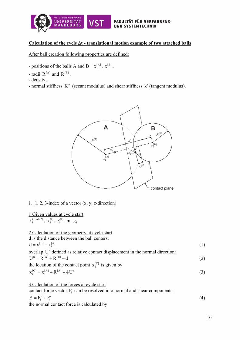
Calculation of the cycle t - translational motion example of two attached balls After ball creation following properties are defined: - positions of the balls A and B ]A[
ix , ]B[ix ,
- radii ]A[R and ]B[R , - density, - normal stiffness nK (secant modulus) and shear stiffness sk (tangent modulus). i .. 1, 2, 3-index of a vector (x, y, z-direction) 1 Given values at cycle start
)2/tt(ix , )t(
ix , )t(iF , m, ig
2 Calculation of the geometry at cycle start d is the distance between the ball centers:
]A[i
]B[i xxd (1)
overlap nU defined as relative contact displacement in the normal direction: dRRU ]B[]A[n (2)
the location of the contact point ]C[ix is given by
n21]A[]A[
i]C[
i URxx (3)
3 Calculation of the forces at cycle start contact force vector iF can be resolved into normal and shear components:
si
nii FFF (4)
the normal contact force is calculated by

17
nnni UKF (5)
The new shear contact force is found by summing the old shear force existing at the start of the time step with the shear force-increment s
iF . If the slip model is active the shear force
will be corrected below smaxF when it is above:
nsi
si
si FFFF (6)
The shear force-increment siF will be found by the following equations (7-10):
]A[]C[
i]B[]C[
ii xxV contact velocity iV (relative motion at the contact) (7) si
nii VVV the contact velocity can be resolved into normal and shear components (8)
tVU si
si shear displacement-increment over a time step of t (9)
si
ssi UkF shear force-increment (10)
The contribution of the final contact force (4) to the resultant force on the two balls in contact is given:
i]A[
i]A[
i FFF (11)
i]B[
i]B[
i FFF (12) ]A[
iF and ]B[iF are the resultant force, the sum of all externally applied forces acting on the two
particles. 4 Calculation at the middle (velocity) and end (position) of the time interval
ix is calculated at the mid-intervals 2/tnt , while iii Fandx,x are computed at the primary intervals of tnt .
)gx(mF iii (13)
)2/tt(i
)2/tt(i
)t(i xx
t
1x
(14)
Insert (13) into (14) and solving for the velocities at time )2/tt( result in
tgm
Fxx i
)t(i)2/tt(
i)2/tt(
i
(15)
Finally, the velocities in (15) are used to update the position of the particle center as txxx )2/tt(
i)t(
i)tt(
i (16)

18
Time steps The computed solution produced by equations (1-16) will remain stable only if the timestep does not exceed a critical timestep. A simplified procedure is implemented in PFC2D to estimate the critical timestep at the start of each cycle. The actual timestep used in any cycle is taken as a fraction of this estimated critical value. This fraction can be specified using the SET safety_fac command.
k/mtcrit (17)
where k is the stiffness of each spring and m the mass of each ball.
Example: s10)m/N10/(kg1t 48crit
Freie ungedämpfte Federschwingung
xmkx 0 xm
kx
020 xx
Es ist:
mk /0 kmT /2
m
k, 0
0 x
FF FT
m
statische Ruhelage Umlenkpunkt
FF ... Federkraft FT ... Trägheitskraft

19
Differential Density Scaling Inertial masses are multiplied by a factor, different for each ball, so that a unit timestep is obtained. Gravitational masses are unaffected. Normal unscaled operation Differential density scaling SET dt auto (default) SET dt dscale New different timesteps are calculated before each cycle step, hence the calculation time for many particles is long.
Only one timestep ist calculated for a particle arrangement befor cycling many times and keep uniform until particle arrangement changes. Hence the general calculation time is reduced.
Provides a true dynamic solution that is valid for both steady- and non-steady-state conditions.
If one is interested only in obtaining the steady-state solution, in which all particle accelerations are zero, corresponding to either static equilibrium or steady flow, differential density scaling may be used to reduce the total number of cycles required to reach the steady-state condition. Only the final steady-state solution is valid; transient states do not represent the true dynamic behaviour of the system. For path-dependent phenomena that involve development of mechanisms, this may result in an unrealistic steady-state solution. Reduce the total number of cycles required to reach the steady-state condition.
Fi is the resultant force, the sum of all externally applied forces acting on the particle:
)gx(mF iii
The inertial mass of each particle is modified at the start of each cycle such that the stability criterion of (17) is satisfied with a timestep of unity:
ig
ii
i g)m(x)m(F where mi and mg are the inertial and gravitational masses, respectively; mg is always equal to the actual mass of the particle and, in the absence of differential density scaling, mi = mg.
The finite-difference expressions for the particle velocities:
tgm
Fxx i
)t(i)2/tt(
i)2/tt(
i
tgm
m
m
Fxx ii
g
i
)t(i)2/tt(
i)2/tt(
i
20
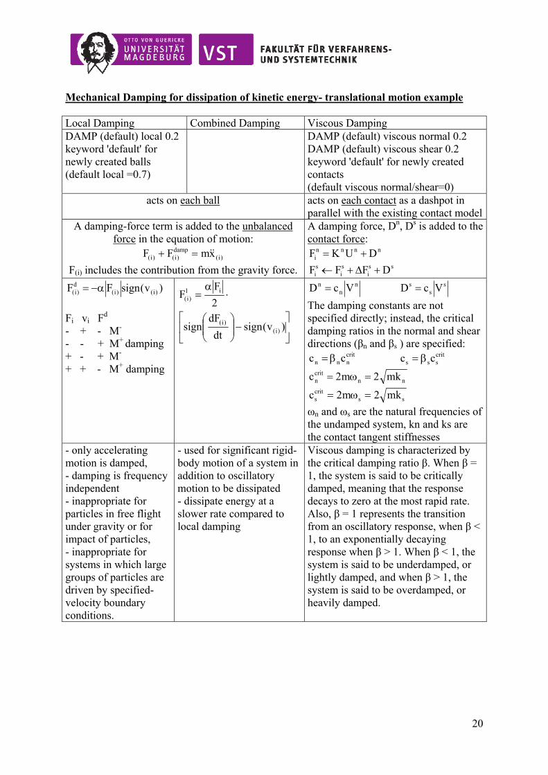
Mechanical Damping for dissipation of kinetic energy- translational motion example Local Damping Combined Damping Viscous Damping DAMP (default) local 0.2 keyword 'default' for newly created balls (default local =0.7)
DAMP (default) viscous normal 0.2 DAMP (default) viscous shear 0.2 keyword 'default' for newly created contacts (default viscous normal/shear=0)
acts on each ball acts on each contact as a dashpot in parallel with the existing contact model
A damping-force term is added to the unbalanced force in the equation of motion:
)i(damp
)i()i( xmFF
F(i) includes the contribution from the gravity force.
A damping force, Dn, Ds is added to the contact force:
nnnni DUKF
ssi
si
si DFFF
)v(signFF )i()i(d
)i(
Fi vi F
d - + - M- - - + M+ damping + - + M- + + - M+ damping
2
FF il
)i(
)v(sign
dt
dFsign )i(
)i(
nn
n VcD
ss
s VcD
The damping constants are not specified directly; instead, the critical damping ratios in the normal and shear directions (βn and βs ) are specified:
critnnn cc crit
sss cc
nncritn mk2m2c
sscrits mk2m2c
ωn and ωs are the natural frequencies of the undamped system, kn and ks are the contact tangent stiffnesses
- only accelerating motion is damped, - damping is frequency independent - inappropriate for particles in free flight under gravity or for impact of particles, - inappropriate for systems in which large groups of particles are driven by specified-velocity boundary conditions.
- used for significant rigid-body motion of a system in addition to oscillatory motion to be dissipated - dissipate energy at a slower rate compared to local damping
Viscous damping is characterized by the critical damping ratio β. When β = 1, the system is said to be critically damped, meaning that the response decays to zero at the most rapid rate. Also, β = 1 represents the transition from an oscillatory response, when β < 1, to an exponentially decaying response when β > 1. When β < 1, the system is said to be underdamped, or lightly damped, and when β > 1, the system is said to be overdamped, or heavily damped.
21
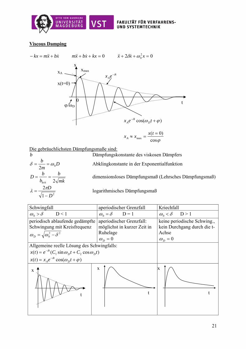
Viscous Damping
xbxmkx 0 kxxbxm 02 20 xxx
Die gebräuchlichsten Dämpfungsmaße sind: b Dämpfungskonstante des viskosen Dämpfers
Dm
b02
Abklingkonstante in der Exponentialfunktion
mk
b
b
bD
krit 2 dimensionsloses Dämpfungsmaß (Lehrsches Dämpfungsmaß)
21
2
D
D
logarithmisches Dämpfungsmaß
Schwingfall aperiodischer Grenzfall Kriechfall
0 D < 1 0 D = 1 0 D > 1
periodisch ablaufende gedämpfte Schwingung mit Kreisfrequenz
220 D
aperiodischer Grenzfall: möglichst in kurzer Zeit in Ruhelage
0D
keine periodische Schwing., kein Durchgang durch die t-Achse
0D Allgemeine reelle Lösung des Schwingfalls:
)cossin()( 21 tCtCetx DDt
)cos()( textx Dt
A
xA
x(t=0)
/D
xmax
)cos( tex D
tA
cos
)0(max
txxxA
t
Aex
t 0
x
t t
x x
t
x