1

Structural and Multidisciplinary Optimization May 2013, Volume 47, Issue 5, pp 765-781

Simulation-Based Time-Dependent Reliability Analysis for Composite Hydrokinetic Turbine Blades

Zhen Hu, Haifeng Li, Xiaoping Du1, K. Chandrashekhara Department of Mechanical and Aerospace Engineering

Missouri University of Science and Technology, Rolla, MO, USA Abstract

The reliability of blades is vital to the system reliability of a hydrokinetic turbine. A time-dependent reliability analysis methodology is developed for river-based composite hydrokinetic turbine blades. Coupled with the blade element momentum theory, finite element analysis is used to establish the responses (limit-state functions) for the failure indicator of the Tsai-Hill failure criterion and blade deflections. The stochastic polynomial chaos expansion method is adopted to approximate the limit-state functions. The uncertainties considered include those in river flow velocity and composite material properties. The probabilities of failure for the two failure modes are calculated by means of time-dependent reliability analysis with joint upcrossing rates. A design example for the Missouri river is studied, and the probabilities of failure are obtained for a given period of operation time. Keywords: reliability, composite, hydrokinetic turbine, time-dependent

1. Introduction

River-based hydrokinetic turbines extract kinetic energy from flowing water of a stream, river, or current [1, 2]. They have similar working principles as wind turbines. The main difference between hydrokinetic turbines and wind turbines is their working environment. The density of water, in which hydrokinetic turbines are put into operation, is about 800 times higher than that of air. Hydrokinetic turbines are advantageous over conventional hydro-power and wind power in the following aspects [3]: A hydrokinetic turbine does not alter natural pathways of rivers; its energy extraction is much higher than the other renewable power technologies; it requires less civil engineering work and introduces less hazards to the environment; the application of

1 Corresponding author, 400 West 13th Street, Toomey Hall 290D, Rolla, MO 65401, U.S. A., Tel:1-573-341-7249, email: dux@mst.edu

2

hydrokinetic turbines is more flexible. Due to the significant advantages of hydrokinetic turbines, this technology has attracted increasing attention of researchers in recent years [4, 5].

As the most important part of the hydrokinetic turbine system, the turbine blade has a high requirement for its performance and strength [6]. Composite materials offer several advantages, such as high ratio of strength to weight, resistance to corrosion, excellent fatigue resistance, and design flexibility. These make composite materials an attractive choice for the construction of turbine blades. Besides, applications of composite materials in the marine and ocean engineering demonstrated that the load-induced deformations of composite elliptic hydrofoils can delay cavitation inception while maintaining the overall lift and drag [7].

Due to the complex manufacturing process, the material properties of composites tend to be more random than metallic materials [8]. For instance, the overall performance of composite turbine blades can be affected by fiber misalignments, voids, laminate properties, boundary conditions and so on [9-11]. There are also many uncertain factors existing in the working environment of turbines and composite structures. In recent years, efforts have been made to reduce the effects of uncertainties on the performance of composite structures and turbine blades. For example, Toft and Sørensen [12] established a probabilistic framework for design of wind turbine blades by adopting a reliability-based design approach. Val and Chernin [13] assessed the reliability of tidal turbine blades with respect to the failure in bending. Motley [14] presented a reliability-based global optimization technique for the design of a marine rotor made of advanced composite. Similarly, Young et al. [8] used a reliability-based design and optimization methodology for adaptive marine structures. They mitigated the influence of composite material uncertainty on the performance of self-adaptive marine rotors. Christopher and Masoud [15] applied the probabilistic design modeling and reliability-based design optimization methodology to the optimization of a composite submarine structure. More developments about the probabilistic design method in the design and optimization of composite structures can be found in [16].

The most commonly used methods for the probabilistic design of composite structures and turbine blades can be classified into two categories: reliability-based design optimization (RBDO) and the inverse reliability design (IRD). RBDO is a methodology that ensures the reliability is satisfied at a desired level by introducing the reliability constraints into the design optimization framework [17]. IRD identifies the design loading using the inverse reliability analysis method [18]. Even though the existing RBDO and IRD methods can be employed for the design of regular composite structures and wind turbine blades, it is hard to use them to guarantee the reliability of composite hydrokinetic blades over the service life. The reason is that most existing RBDO and IRD methods employed for the design of composite structures and turbine blades are based on time-invariant reliability analysis, while the uncertainties in hydrokinetic turbine blades always change with time. For instance, the river flow climate, which governs the loading of turbine blades, is a stochastic process with strong auto-correlations [19, 20]. This means that the monthly river flow velocity has much longer memory than the wind climate and that the reliability of hydrokinetic turbine blades is time dependent. The Monte Carlo simulation (MCS) can be used for time-dependent reliability analysis, but it is computationally expensive. Efficient time-dependent reliability analysis methods, therefore, need to be employed for the probabilistic design of composite hydrokinetic turbine blades.

In the past decades, many methods have been proposed for the time-dependent reliability analysis, such as the Gamma distribution method, Markov method [21], and the upcrossing rate

3

method [22]. Amongst the above methods, the upcrossing rate method is the most widely used one [23, 24], which has been applied to the time-dependent reliability analysis for function generator mechanism [25], steel beam under stochastic loading [26], and hydrokinetic turbine blades [27]. As the method in [25-27] is based on the simple Poisson assumption, it cannot well take into account the correlation of river velocities at different time instants. A more accurate method called the first order reliability method with joint upcrossing rate (JUR/FORM) has been recently developed [28]. This method combines the joint upcrossing rates (JUR) with First Order Reliability Method (FORM). It is suitable for the time-dependent reliability analysis of composite hydrokinetic turbine blades in this work.

The objective of this work is to develop a reliability analysis model for composite hydrokinetic turbine blades by quantifying the effects of uncertainties in river flow velocity and composite material properties on the performance of hydrokinetic turbine blades over the design life. It is an improved work of the reliability analysis method of hydrokinetic turbine blades presented in [27]. The finite element method (FEM) is employed to analyze the performances of the hydrokinetic turbine blade. The JUR/FORM reliability analysis method is adopted for reliability analysis. A three-blade horizontal-axis hydrokinetic turbine system developed for the Missouri river is studied. The probabilities of failure of turbine blades according to the Tsai-Hill failure criterion and excessive deflections are analyzed.

The remainder of the paper is organized as follows: In Section 2, we provide the state of the art of the time-dependent reliability analysis methods. Following that, in Section 3, we analyze uncertainties that affect the performance of composite hydrokinetic turbine blades and study the potential failure modes of turbine blades. In Section 4, we discuss the way of modeling the loading of turbine blades and the methods employed to establish the limit-state functions. A design example is given in Section 5 and conclusions are made in Section 6.

2. The State of the Art of Time-Dependent Reliability Analysis Methods Reliability analysis problems can be divided into the following two categories: ⋅ Time-invariant reliability problems with random variables ⋅ Time-dependent reliability problems with stochastic processes In the past decades, many methods have been developed for time-invariant reliability

problems. These methods include FORM, Second Order Reliability Analysis Method (SORM), and Importance Sampling Method (ISM).

For the time-dependent reliability analysis problems, such as the reliability analysis of composite hydrokinetic turbine blades under stochastic river flow loading, are much more complicated. To show the complexities, in the following subsections, we first discuss the differences between the two reliability problems and then review several methodologies for time-dependent reliability analysis.

2.1 Time-dependent reliability and time-invariant reliability

Time-invariant reliability does not change over time while the time-dependent reliability does. Let a general limit-state function be

), )( , (G tg t= X Y (1)

4

in which 1 2[ , , , ]nX X X=X is a vector of random variables, and 1 2) [ ( ), ( ), ( )]( mY t Yt t Y t=Y is a vector of stochastic processes.

(a) Time-dependent reliability For the general limit-state function in Eq. (1), the response variable G is a random variable

at any instant of time. Let the threshold of a failure be e . If a failure occurs when ( , ( ), )G g t t e>= X Y , the time-dependent probability of failure over a time interval 0[ , ]st t is

given by

{ }0 0( , ) Pr ( , ( , [ , ]))f s sP t t g t e t t t= ∃> ∈X Y (2)

where {}Pr ⋅ stands for the probability. The corresponding time-dependent reliability is given by

{ }0 0( , ) Pr ( , ( ) , [ , ])s sR t t g t e t t t= ∀< ∈X Y (3)

The time-dependent reliability tells us the likelihood that no failure will occur over a time period.

(b) Time-invariant reliability At a specified time instant it , the reliability is given by

{ }( ) Pr ( , )( )i iR t g t e= <X Y (4)

This reliability is called instantaneous reliability or time-invariant reliability. It is the probability that the response variable is not greater than the threshold at it , thereby not in the failure region, regardless whether a failure has occurred or not prior to it . It is meaningful for only time-invariant limit-state functions ( )g X , which does not depend on time, resulting a constant reliability. For a time-dependent problem over 0[ , ]st t , the instantaneous reliability is only used for the initial reliability at 0t t= .

The methods for the time-invariant reliability, however, may not be directly used to calculate the time-dependent reliability. The major reason is that the time-dependent reliability is defined over a time period, which consists of infinite numbers of time instants where the response variables are dependent. 2.2 Methodologies for time-dependent reliability analysis

2.2.1. MCS for time-dependent reliability analysis The implementation of MCS for time-dependent reliability analysis is quite different from

that for time-invariant one. The differences lie on the ways of counting failure events and generating random samples.

If stochastic processes are involved, we need at first to generate their trajectories (sample traces). Since a trajectory is a continuous function of time, we need to use many discretization points (time instants) to accurately represent the function. At each of the time instants, a stochastic process is a random variable and the random variables at all the time instants are usually dependent. As a result, the random samples are stored in a two-dimensional array – one is indexed by time instants, and the other is indexed by random trajectories. For a time-invariant

5

problem, the samples are represented by just a one-dimensional array because no time is involved. The size of the samples of a time-dependent problem is therefore much higher than that of a time-invariant one.

After the samples are generated, a limit-state function will be evaluated at all the sample points. Compared to a time-invariant problem, the number of function calls for a time-dependent problem will be much higher because of the above reason. By comparing the value of a limit-state function against the failure threshold, we will know if a failure occurs. If the limit-state function value is greater than the threshold at any discretized time instant, we consider the event as a failure. The details of MCS for time-dependent reliability analysis are provided in Appendix A.

Due to its high computational cost, MCS is not practically used for time-dependent reliability analysis, but may be used as a benchmark for the accuracy assessment for other reliability analysis methods.

2.2.2. Poisson assumption based upcrossing rate method Given its high efficiency, the Poisson assumption based upcrossing rate method has been

widely used [25-27]. With this method, the time-dependent probability of failure over time interval 0[ , ]st t is computed by

{ }0

0 0( )]( , ) 1 [1 exp ( )st

ff s tp t t p t v t dt+= − − −∫ (5)

in which ( )v t+ is the upcrossing rate at time t, and 0( )fp t stands for the instantaneous probability of failure at the initial time.

It is difficult to obtain the upcrossing rate ( )v t+ . One effective way is using FORM. FORM transforms random variables { ), ( }tX Y into the standard normal variables ( ) [ , ( )]t t= X YU U U . Then the limit state function becomes ( ( ), )G g t t= U [25]. After the linearization of the limit-state function at the Most Probable Point (MPP) *( )tu , the upcrossing rate ( )v t+ is computed using the Rice’s formula [29, 30] as follows:

( )( ) ( ) ( ) { ( ( ) / ( )) [ ( ) / ( )] ( ( ) / ( ))}v t t t t t t t t tω φ β φ β ω β ω β ω+ = − Φ − (6)

where ( )φ ⋅ and ( )Φ ⋅ represent the probability density function (PDF) and cumulative distribution function (CDF) of a standard normal random variable, respectively, and

*( ) ( )t tβ = u (7)

in which ⋅ stands for the magnitude of a vector.

( )tω is given by

212( ) ( ) ( ) ( ) ( , ) ( )T Tt t t t t t tω = +α α α C α

(8) where

* *( ) ( ( ), ) / ( ( ), )t t t t t= ∇ ∇α g u g u (9)

and

6

12

1 212 1 2 21 1 2

2

1 2 ( ) ( )

( , ) 0( , ) ( , )

( , )0m

Y

Y

n m n m

t tt t

t t t t

t tt t

ρ

ρ

+ × +

∂ ∂ ∂

= = ∂

∂ ∂

0 0 0

0C C

0

(10)

in which ( , )iY t tρ is the autocorrelation coefficient function of stochastic process iY .

( )tα and ( )tβ are the derivatives of ( )tα and ( )tβ , respectively. Even if the Poisson assumption based upcrossing rate method has been widely used, large

errors have been reported for this method by Madsen etc. [31][32][33][34]. One of the main error sources is the Poisson assumption, which assumes that the events that the response upcrosses the failure threshold are completely independent from each other. This assumption does not hold for many cases because there are always some correlations between the failure events and failures may occur in clusters. To overcome this drawback, Madsen [31] proposed a method to consider the correlation between two time instants of a Gaussian process. His method focuses on only Gaussian processes. Vanmarcke [32] has made some empirical modifications to the Poisson assumption based method. His modifications, however, are limited to stationary Gaussion process. Most recently, Singh [34] has established a “composite” limit-state function method, which can accurately estimate the time-dependent reliability problems with limit-state functions in a form of ( ),G tg= X , where there are no input stochastic processes. The JUR/FORM [28] method has recently been developed by extending Madsen’s method [31] for more general problems with both random variables and non-stationary stochastic processes. We next review the main idea of the JUR/FORM.

2.2.3. JUR/FORM JUR/FORM aims to release the Poisson assumption by considering the correlations between

the limit-state function at two time instants. It can be applied to general problems with both random variables and stochastic processes. Since it is based on FORM, it is much more efficient than MCS while the accuracy is higher than the traditional upcrossing method. With this method, the time-dependent probability of failure 0( , )f sp t t is computed by

{ } { } ( )1

00 0 0 0 0( ) Pr ( , ( Pr ( , (, ), ) ), ) st

f s Ttp t t g t t e g t t e f t dt= > + < ∫X Y X Y (11)

where 1( )Tf t is the PDF of the first-time to failure. { }0 0Pr ( , ,( ) )g t t e>X Y is the probability of

failure at the initial time, and { } ( )1

00 0), )Pr ( , ( st

Ttg t t e f t dt< ∫X Y

is the probability of failure over

0[ ], st t given that no failure occurs at the initial time.

( )1Tf t can be obtained by solving the following integral equation [31]:

1 1

0

( ) ( ) ( , ) ( ) / ( )t

T Ttv t f t v t f v dt t t t+ ++ += + ∫ (12)

7

in which ( )v t+ is given in Eq. (6), and ( , )v t t++ stands for the joint probability that there are upcrossings at both t and t . The equations for ( , )v t t++

are given in Appendix B.

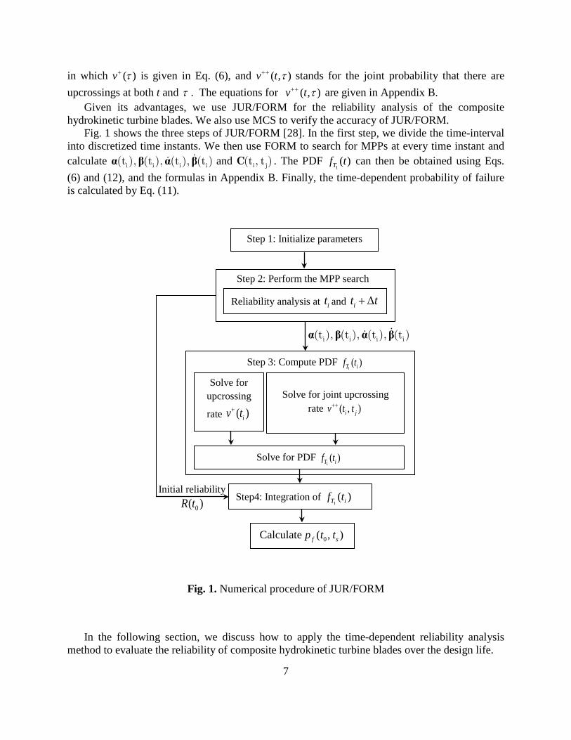
Given its advantages, we use JUR/FORM for the reliability analysis of the composite hydrokinetic turbine blades. We also use MCS to verify the accuracy of JUR/FORM.

Fig. 1 shows the three steps of JUR/FORM [28]. In the first step, we divide the time-interval into discretized time instants. We then use FORM to search for MPPs at every time instant and calculate α β α βi i i i(t ), (t ), (t ), (t ) and i j(t , t )C . The PDF

1( )Tf t can then be obtained using Eqs.

(6) and (12), and the formulas in Appendix B. Finally, the time-dependent probability of failure is calculated by Eq. (11).

Fig. 1. Numerical procedure of JUR/FORM

In the following section, we discuss how to apply the time-dependent reliability analysis method to evaluate the reliability of composite hydrokinetic turbine blades over the design life.

Step 1: Initialize parameters

Reliability analysis at it and it t+ ∆

Step 2: Perform the MPP search

Solve for upcrossing

rate ( )iv t+

Solve for joint upcrossing

rate ( , )i jv t t++

Solve for PDF 1( )T if t

Step4: Integration of 1( )T if t

Step 3: Compute PDF 1( )T if t

α β α βi i i i(t ), (t ), (t ), (t )

Calculate 0( , )f sp t t

Initial reliability

0( )R t

8

3. Uncertainty and Failure Modes Analysis for Composite Hydrokinetic Turbine Blades

3.1 Uncertainty analysis 3.1.1 River flow velocity

Due to the natural variability, the river flow velocity is the major uncertainty inherent in the working environment of hydrokinetic turbine blades. It is directly related to the safety of the turbine blade. Analyzing the uncertainty of the river flow velocity is critical to the reliability analysis of hydrokinetic turbine blades. The river flow velocity, however, is difficult to be modeled exactly since it varies both in space and time. To present the variation of river flow velocity over space and time, we need many historical river flow velocity data at different locations of the river cross section. This kind of data is not available at most of the time. In order to overcome this limitation, Hu and Du [27] proposed to present the river flow velocity in the form of river discharge, of which the data have been recorded for many rivers. With the river discharge and the assumption that the shape of a river bed is a rectangle, the cross section average river flow velocity is calculated by the Manning-Strickler formula as follows [35-37]:

1 2/3 1/2( ) ( )rv t n Q t S−= (13)

in which ( )v t is the river water flow velocity (m/s) , rn is the river bed roughness, S is the river slope (m/m), and ( )Q t is given by [27, 37]

0.898

0.341 0.557

0.946( )0.698 2.71

m

m m

dQ td d

=+

(14)

where md is the monthly discharge of the river 3(m /s) .

The distribution of md is lognormal [38, 39], and its CDF is given by

ln( ) ( )

( )( )

m

m

m

m DD m

D

d tF d

tm

σ

−= Φ

(15)

in which ( )mD tm

and ( )

mD tσ are the mean and standard deviation of ( )ln md , respectively. These

two parameters are time-dependent because the river discharge varies seasonally. The autocorrelation coefficient of the normalized and standardized monthly river discharge is approximated by [20, 40]

2

2 11 2( , ) exp

mDt tt tρζ

−= −

(16)

9

where ζ is the correlation length. Therefore, after normalization and standardization, the monthly river discharge can be presented by its underlying Gaussian process with autocorrelation coefficient function given in Eq. (16).

3.1.2 Uncertainties in composite materials The hydrokinetic turbine blade is made of fiberglass/epoxy laminates with [0/90/0/90/0]s

symmetric configurations. Due to the natural variability in laminate properties, fiber misalignment, and the fabrication process of composite materials, uncertainties exist in the stiffness of composite materials. Herein, four variables are represented by probability distributions. These random variables are E11 and E22 (E33) (elastic modulus along direction 1, 2 and 3), G12 (G13), and G23 (shear modulus). All the random variables are normally distributed. As suggested in [8], a 2% coefficient of variation was assigned to the material parameters of the composite material as shown in Table 1. The coefficient of variation is the ratio of the standard deviation to the mean of a random variable.

Table 1. Distributions of random variables of the composite material

Variable Value Distribution type Mean Coefficient of variation

Young’s modulus E11=45.6 GPa 0.02 Gaussian E22=E33=16.2 GPa 0.02 Gaussian

Shear Modulus G12= G13=5.83 GPa 0.02 Gaussian G23=5.786 GPa 0.02 Gaussian

After identifying the uncertainties in the composite hydrokinetic turbine blade, we analyze the

potential failure modes that may occur during the operation of turbine blades.

3.2 Failure modes of composite hydrokinetic turbine blades The failure modes of wind turbine blades have been reported in literature. They can be used

as a reference for analyzing hydrokinetic turbine blades because both wind and hydrokinetic turbine blades share similar working principles. For wind turbine blades, the commonly studied failure modes include failures due to fatigue [41, 42], extreme stresses [43, 44], excessive deflections [45], corrosion [46, 47], and so on. Based on the studied failure modes, in this work, we mainly focus on the failure modes with respect to the Tsai-Hill failure criterion and excessive deflection. The major reason of doing this is that the extreme stress and deflection can be obtained from static analysis and that the two failure modes can be analyzed using the same kind of reliability analysis method.

The fatigue of turbine blades is also critical to the reliability of a turbine system. The fatigue reliability analysis requires a stress cycle distribution of blades obtained from a large number of

10

simulations or experiments. It also needs stochastic S-N curve to account for uncertainties in material fatigue tests. It is a much more challenging task and will be one of our future works.

3.2.1 The Tsai-Hill failure criterion for composite turbine blades For plane stresses, the failure indicator of the Tsai-Hill criterion is

2 2 21 1 2 2 122 2 2 2indL L T LT

fs s s sσ σ σ σ t

= − + + (17)

where 1σ , 2σ and 12t are local stresses in a lamina with reference to the material axes. Ls , Ts and LTs are the failure strengthes in the principal material directions. Ls stands for the longitudinal strength in fiber direction (direction 1), Ts denotes transverse strength in matrix direction (direction 2), and LTs indicates the in-plane shear strength (in plane 1-2).

If 1 0σ > , use longitudinal tensile strength for Ls ; if 2 0σ > , use transverse tensile strength for

Ts ; otherwise, use the compressive strength for Ls and Ts . To determine whether the composite blade laminate will fail due to applied loading, the method first calculates stresses across the different plies, followed by applying the Tsai-Hill interactive failure criterion based on these stress levels. The composite blade laminate is considered to fail when a first ply fails. This point of failure is the first ply failure (FPF) [48, 49], beyond which the laminate may still carry the load. For a safe design, the composite laminates should not experience stress high enough to cause FPF. Fig. 2 shows a failure evaluation of hydrokinetic turbine blade using the Tsai-Hill criterion in ABAQUS.

Fig. 2. Blade failure evaluation under hydrokinetic loadings (based on the Tsai-Hill criterion)

The limit-state function with respect to the Tsai-Hill failure criterion is defined by

( )1 0, ( ), ( , ( ,) [) , ]b b ind b b allow sg t t f t t f t t t= − ∈X Y X Y (18)

where ( , ( ) ),ind b bf t tX Y is the failure indicator of the composite blade based on the Tsai-Hill

criterion, allowf is the allowable value, 11 22 12 23[ , , , ]b E E G G=X is the vector of random variables,

and ( ) [ ( )]b t v t=Y is the vector of stochastic process. When ( ), ( ), 0b bg t t >X Y , a failure occurs

based on the Tsai-Hill criterion.

11

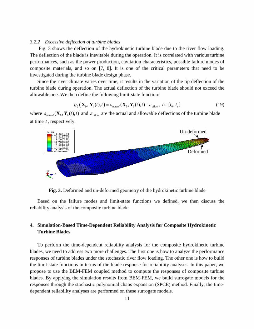
3.2.2 Excessive deflection of turbine blades Fig. 3 shows the deflection of the hydrokinetic turbine blade due to the river flow loading.

The deflection of the blade is inevitable during the operation. It is correlated with various turbine performances, such as the power production, cavitation characteristics, possible failure modes of composite materials, and so on [7, 8]. It is one of the critical parameters that need to be investigated during the turbine blade design phase.

Since the river climate varies over time, it results in the variation of the tip deflection of the turbine blade during operation. The actual deflection of the turbine blade should not exceed the allowable one. We then define the following limit-state function:

( )2 0, ( ), ( , ( , , [ ]) ,)b b actual b b allow sg t t t t t t tε ε= − ∈X Y X Y (19)

where )( , )( ,actual b b t tε X Y and allowε are the actual and allowable deflections of the turbine blade at time t , respectively.

Fig. 3. Deformed and un-deformed geometry of the hydrokinetic turbine blade

Based on the failure modes and limit-state functions we defined, we then discuss the reliability analysis of the composite turbine blade.

4. Simulation-Based Time-Dependent Reliability Analysis for Composite Hydrokinetic Turbine Blades To perform the time-dependent reliability analysis for the composite hydrokinetic turbine

blades, we need to address two more challenges. The first one is how to analyze the performance responses of turbine blades under the stochastic river flow loading. The other one is how to build the limit-state functions in terms of the blade response for reliability analyses. In this paper, we propose to use the BEM-FEM coupled method to compute the responses of composite turbine blades. By applying the simulation results from BEM-FEM, we build surrogate models for the responses through the stochastic polynomial chaos expansion (SPCE) method. Finally, the time-dependent reliability analyses are performed on these surrogate models.

Un-deformed

Deformed

12

4.1 Construction of surrogate models

4.1.1 BEM-FEM coupled method The blade element momentum theory (BEM), proposed by Glauert in 1935, has been widely

used to calculate the load of turbine blades. It is applicable to estimate the steady loads, the thrust and power for different settings of speed, rotational speed and pitch angle of turbines [50]. Since it is based on the momentum theory and the local events taking place at the blade elements, it may not be as accurate as that from the 3-dimentional computational fluid dynamics (CFD) simulations. However, the BEM calculation is much faster than the CFD simulation. Given its high efficiency and many corrections to the original model, BEM provides engineers with an effective way of approximating the aerodynamic/hydrodynamic loadings on turbine blades.

In the present work, we employ BEM to compute the loadings on the composite hydrokinetic turbine blades in reliability analysis. The load produced by BEM serves as the input of FEM, which generates the stress distribution of the turbine blade. We refer this procedure as the BEM-FEM coupled method.

Fig. 4 shows the flowchart of the BEM-FEM coupled method. For BEM, we assume that there is no-radial-dependency among blade elements. However, we incorporate the Prandtil’s tip loss, Glauert correction, and hub loss into the model to ensure reliable results. The hydrodynamic loadings obtained from BEM codes have been validated with Blade Tidal, which is a design tool for tidal current turbines [51].

Fig. 4. Flowchart of the BEM-FEM

Hydrofoil Datasheet

River Velocity

Blade Geometry (Radius, chord,

twist, pitch, etc.) Bending Moments,

Forces, Power Coefficient

Blade Stress and Deflection (Critical

region identification, failure evaluation)

Post Process

Blade Structure (Material, number of plies,

ply orientation, stacking sequence, ply thickness)

BEM

FEM

MATLAB

MATLAB

ABAQUS

13

Fig. 5 presents the finite element mesh of the blade, which is divided into eight stations, and each station is applied with concentrated hydrodynamic forces on the blade surface using multipoint constraints (MPC) technique.

Fig. 5. Finite element mesh of the blade

If BEM-FEM is directly employed for the time-dependent reliability analysis, the efficiency will be very low, as the number of FEM runs is much higher than that of the time-invariant reliability analysis. Since the time-dependent reliability analysis will be later integrated into an optimization framework, the direct use of BEM-FEM may not be affordable in terms of computational efforts. Therefore, we construct surrogate models based on limited and selected BEM-FEM analyses. In the next section, we will introduce a method to construct the surrogate models based on the FEM simulations.

4.1.2 SPCE method Since the uncertainties are all modeled by random variables, we use the SPCE method to get

the surrogate models for the two limit-state functions. As an efficient tool for multi-disciplinary design optimization (MDO) in various engineering applications, SPCE has drawn much attention in the past decades. With SPCE, the chaos expansion for a response Z is given by [52, 53]

0

( )P

i ii

Z χ=

= Γ∑ ξ (20)

where iχ are deterministic coefficients, ( )iΓ ξ are the i-th order random basis functions,

1 2[ , , ]nξ ξ ξ=ξ is a vector of independent standard random variables, and P is the number of terms. The total number of terms for a complete polynomial chaos expansion of order p and n random variables is given by

( )!1! !

n pPn p+

+ = (21)

The use of independent standard random variables in Eq. (20) is critical because it allows decoupling of the multidimensional integrals in a mixed basis expansion [54]. ( )iΓ ξ are multivariable polynomials, which involve products of one-dimensional polynomials. For the expansion of a response with different kinds of random variables, mixed bases will be used. There are different kinds of basis functions for different uncertainty distributions [52]. For a normal (Gaussian) uncertain variable, the ideal basis function is the Hermit polynomial. For a uniform or exponential distribution, the ideal basis function is Legendre or Laguerre polynomial.

14

In this work, the point collocation method is applied to get the deterministic coefficients iχ in Eq. (20). For the point collocation method, sampling of input random variables is the key to ensure the efficiency and accuracy of the approximation. The most commonly used sampling methods include the Random Sampling (RS), Latin Hypercube Sampling (LHS), and Hammersley Sampling (HS) [55]. We use HS to generate samples for input random variables because it is capable of providing better uniformity properties over multi-dimensional space than LHS and RS.

For the time-dependent reliability analysis of composite hydrokinetic turbine blades, the uncertainties in the material are modeled as Gaussian random variables, which can be expanded using the Hermit polynomial basis. The flow velocity is a stochastic process that varies randomly over time. As a result, at different time instants, the velocity distributions will be different. There is no single distribution we could use for the expansion. Therefore, we regard the flow velocity as a variable with unknown distribution and then treat it with a uniform distribution bounded by the cut-out and cut-in velocity as shown in Fig. 6. This treatment is similar to expand a general variable. As shown in the example in this paper, this treatment works well for the reliability analysis of turbine blades. For stochastic polynomial chaos expansion, we therefore use the Hermit polynomials for E11, E22 (E33), G12 (G13), and G23; and Legendre polynomials for the river velocity. For multivariate basis functions, the mixed bases are used for expansion.

Fig. 6. Distribution of river flow velocity

With the expansion order of two, the polynomial chaos expansion model for the studied problem in this work is given by

20 4 4

0 1 5 1 5 5 1 1 50 1 1

3 4 4

( , ) 1 1 15 2 20 2 51 1 1

( ) ( ) ( ( )) ( ) ( ( ))

( ) ( ) ( ) ( ( ))

s s s s s si i i i i i

k i i

s s si j i j i i

i j i i

Z H L t H L t

H H H L t

χ χ χ χ χ

χ χ χ

+= = =

+= = + =

= Γ = + + +

+ + +

∑ ∑ ∑

∑∑ ∑

ξ ξ ξ ξ ξ

ξ ξ ξ ξ (22)

PDF

inv

outv

1t i

t nt

( )v t

15

, 1, , 4j

j

j Xj

X

xj

m

σ

−= =ξ (23)

and

52 ( )( ) L U

U L

v t v vtv v− −

=−

ξ (24)

in which , 1, , 4j j =ξ , are the standard normal random variables corresponding to material strengths 5 ( )tξ is a normalized uniform random variable bounded in [-1, 1], which is associated with the stochastic process of river velocity ( )v t at time t 1 2 3 4[ , , , ]x x x x=x is a vector of specific values for random variables 11 22 12 23[ , , , ]E E G G

jXm and jXσ are the mean and standard deviation of random variable jX , respectively

Lv is the lower bound of tip river velocity expansion interval Uv is the upper bound of river velocity expansion interval ( ), 1, 2iH i⋅ = , is the ith order Hermit polynomial basis ( ), 1, 2iL i⋅ = , is the ith order Legendre polynomial basis , 1, 2sZ s = , represents the limit-state functions, s=1 for limit-state function 1 in Eq. (18), and s=2 for limit-state function 2 in Eq. (19) , 1, 2 and 0,1, 2, , 20s

i s iχ = = , stand for the deterministic coefficients of the surrogate models. s=1 for surrogate model associated with limit-state function 1 and s=2 for surrogate model associated with limit-state function 2

Assume that pN simulations are performed for the turbine blades at the sample points

generated from HS, the deterministic coefficients , 1, 2 and 0,1, 2, , 20si s iχ = = , are then

solved by the point collocation method as follows:

1 1 1 10 1 20 0

2 2 2 20 1 20 1

200 1 20

( ) ( ) ( ) ( )( ) ( ) ( ) ( )

( ) ( ) ( ) ( )p p p p

ss

ss

sN N N Ns

ZZ

Z

χχ

χ

Γ Γ Γ Γ Γ Γ = Γ Γ Γ

ξ ξ ξ ξξ ξ ξ ξ

ξ ξ ξ ξ

(25)

where 1 2 3 4 5[ , , , , ( )], 1, ,i i i i i ipt i N= =ξ ξ ξ ξ ξ ξ is the ith group of sample points generated from HS,

and ( )s iZ ξ is the blade response of sZ with the ith group of sample points obtained from the simulation.

4.2 Reliability analysis of composite hydrokinetic turbine blades

We assume that the seasonal effects of river flow velocity repeat in the same time periods of any year. This assumption is reasonable given the fact that the Earth circulates around the Sun

16

annually with the same seasonal effects. Based on this assumption, the probability of failures during T-years operation can be calculated by

( ) 1 [1 ( )]i i Tf f ep T p Y= − − (26)

where ( )ifp T is the probability of failure during T years; ( )i

f ep Y is the annual probability of failure. i stands for the two failure modes as follows:

⋅ 1i = for the failure with respect to the Tsai-Hill failure criterion ⋅ 2i = for the failure of excessive deflection

In Eq. (26) the annual probability of failure ( )if ep Y is defined over a time interval [0, ]t ,

where t is equal to one year. The anuual probability of failure ( )if ep Y

can be solved by applying

JUR/FORM given in Section 2 and using the surrogate models in Section 4.1.

4.3 Numerical procedure

In this section, we summarize the numerical implementation of the reliability analysis method discussed above. Fig. 7 depicts the procedure of the implementation.

Fig. 7. Flowchart of simulation-based time-dependent reliability analysis

Step 1: Sample generation: generate the samples of random variables using the Hammersley Sampling method based on their distribution.

Step 2: BEM-FEM coupled analysis: with the input samples from step 1, analyze the failure indicator with respect to the Tsai-Hill failure criterion and deflection of the hydrokinetic turbine blade using BEM-FEM.

Design of Experiment

(Input samples)

Probability of Failure

River Velocity Stochastic Property

Reliability Analysis

(FORM/JUR)

SPCE (Linear regression)

BEM-FEM

(Failure indicator, stress

distribution, deflection)

Turbine Blade Design

Input to BEM-FEM

Output from BEM-FEM

Limit-state function

Stochastic Process

17

Step 3: Design of experiments: construct surrogate models using the outputs from simulations and approximate the responses with the stochastic polynomial chaos expansion method.

Step 4: Reliability analysis: Perform time-dependent reliability analysis by applying the JUR/FORM method.

5. Case study

We studied a one-meter long composite hydrokinetic turbine blade with varying chord lengths, cross sections and an eight-degree twist angle. This blade is for a hydrokinetic turbine system that is intended to put into operation in the Missouri River. During the design process, we evaluated the reliability of the hydrokinetic turbine over a 20-year design period. 5.1 Data

5.1.1 River discharge of the Missouri River Based on the historical river discharge data of Missouri river from 1897 to 1988 at Hermann station, the mean and standard deviation of the monthly river discharge were fitted as functions of t as follows [27]

5

01

( ) [ cos( ) sin( )]m

mean mean meanD i mean i mean

it a a i t b i tm ω ω

=

= + +∑ (27)

5

01

( ) [ cos( ) sin( )]m

std std stdD j std j std

jt a a j t b j tσ ω ω

=

= + +∑ (28)

where

0 1 2 3 4 5

1 2 3 4 5

2335, 1076, 241.3, 61.69, 30.92, 32.38,

57.49, 174.9, 296.2, 213.6, 133.6, 0.5583

mean mean mean mean mean mean

mean mean mean mean meanmean

a a a a a ab b b b b ω

= = − = = = − =

= = − = − = = − = (29)

0 1 2 3 4 5

1 2 3 4 5

1280, 497.2, 145.8, 225.4, 203.1, 99.47,

82.58, 19.06, 178.7, 36.15, 52.47, 0.5887

std std std std std std

std std std std stdstd

a a a a a ab b b b b ω

= = − = = = − =

= − = − = − = = − = (30)

The auto-correlation coefficient function of the normalized and standardized monthly discharge was assumed to be

21 2 2 1( , ) exp{ [20( ) / 3] }

mD t t t tρ = − − (31)

5.1.2 Deterministic parameters for time-dependent reliability analysis

Table 2 presents the deterministic parameters for the reliability analysis, which include the limit states and time step size.

18

Table 2. Deterministic parameters used for reliability analysis

Parameter allowf allowε t∆

Value 1 3.5×10-2 (m) 5×10-3 (month)

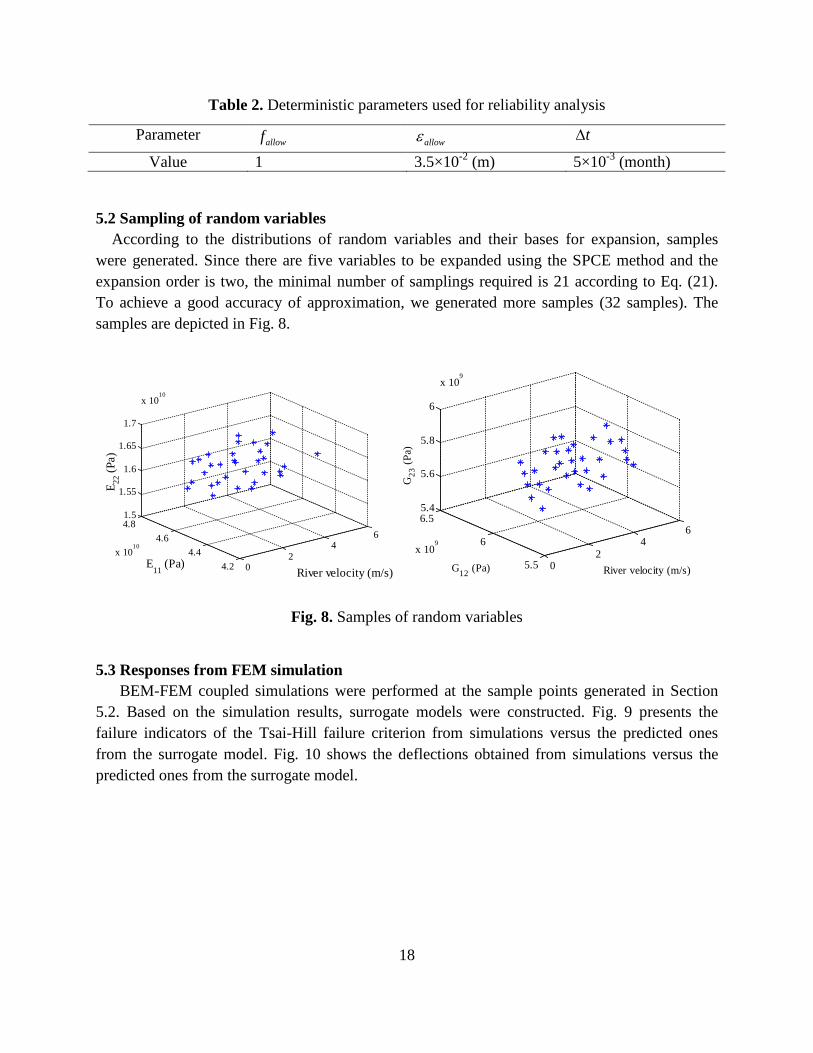
5.2 Sampling of random variables According to the distributions of random variables and their bases for expansion, samples

were generated. Since there are five variables to be expanded using the SPCE method and the expansion order is two, the minimal number of samplings required is 21 according to Eq. (21). To achieve a good accuracy of approximation, we generated more samples (32 samples). The samples are depicted in Fig. 8.

02

46

4.24.4

4.64.8

x 1010

1.5

1.55

1.6

1.65

1.7

x 1010

River velocity (m/s)E

11 (Pa)

E 22 (P

a)

0

24

6

5.5

6

6.5

x 109

5.4

5.6

5.8

6

x 109

River velocity (m/s)G12 (Pa)

G23

(Pa)

Fig. 8. Samples of random variables

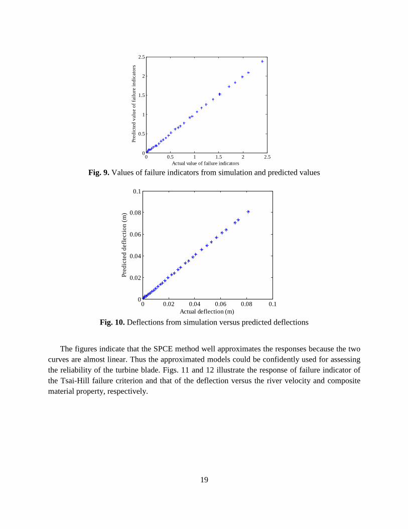
5.3 Responses from FEM simulation BEM-FEM coupled simulations were performed at the sample points generated in Section 5.2. Based on the simulation results, surrogate models were constructed. Fig. 9 presents the failure indicators of the Tsai-Hill failure criterion from simulations versus the predicted ones from the surrogate model. Fig. 10 shows the deflections obtained from simulations versus the predicted ones from the surrogate model.

19

0 0.5 1 1.5 2 2.50

0.5

1

1.5

2

2.5

Actual value of failure indicators

Pred

icte

d va

lue

of fa

ilure

indi

cato

rs

Fig. 9. Values of failure indicators from simulation and predicted values

0 0.02 0.04 0.06 0.08 0.10

0.02

0.04

0.06

0.08

0.1

Actual deflection (m)

Pred

icte

d de

flect

ion

(m)

Fig. 10. Deflections from simulation versus predicted deflections

The figures indicate that the SPCE method well approximates the responses because the two curves are almost linear. Thus the approximated models could be confidently used for assessing the reliability of the turbine blade. Figs. 11 and 12 illustrate the response of failure indicator of the Tsai-Hill failure criterion and that of the deflection versus the river velocity and composite material property, respectively.

20

44.5

55.5

x 1010

0

2

4

60

1

2

3

E11

(Pa)River velocity (m/s)

Failu

re in

dica

tor

Fig.11. Failure indicator for Tsai-Hill failure criterion

44.5

55.5

x 1010

02

460

0.05

0.1

E11

(Pa)River velocity (m/s)

Def

lect

ion

(m)

Fig.12. Deflection of turbine blades

21

5.4 Reliability analysis and results

We first calculated the probability of failure of the hydrokinetic turbine blade over a one-year time period 0[ , ] [0,1]st t = yr. We then computed the probability of failure over the life time

0[ , ] [0, 20]st t = yr using Eq. (26).

5.4.1 Time-dependent probabilities of failure

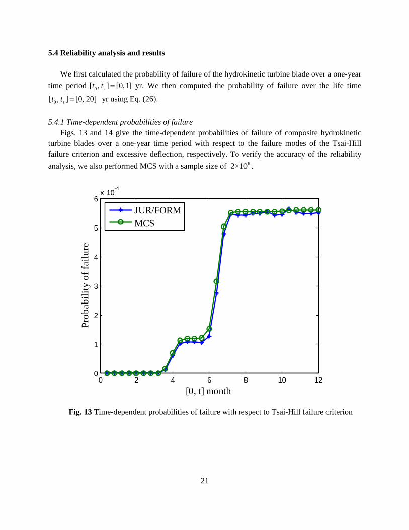
Figs. 13 and 14 give the time-dependent probabilities of failure of composite hydrokinetic turbine blades over a one-year time period with respect to the failure modes of the Tsai-Hill failure criterion and excessive deflection, respectively. To verify the accuracy of the reliability analysis, we also performed MCS with a sample size of 2× 610 .

0 2 4 6 8 10 120

1

2

3

4

5

6x 10

-4

[0, t] month

Prob

abili

ty o

f fai

lure

JUR/FORMMCS

Fig. 13 Time-dependent probabilities of failure with respect to Tsai-Hill failure criterion

22

0 2 4 6 8 10 120

0.5

1

1.5x 10-3

[0, t] month

Prob

abili

ty o

f fai

lure

JUR/FORMMCS

Fig. 14 Time-dependent probabilities of failure with respect to excessive deflection

The results indicate that the accuracy of the reliability analysis from JUR/FORM is good.

The probability of failure for the Tsai-Hill failure criterion is 5.6312×10-4 over a one-year period. The probability of failure due to excessive deflection is 11.0843×10-4 over a one-year time period. The failure mode of the Tsai-Hill failure criterion is less likely to happen than that of excessive deflection for this design. The probabilities of failure for the Tsai-Hill failure criterion and excessive deflection over a 20-year life period are 1.12×10-2 and 2.19×10-2, respectively.

Tables 3 and 4 present the actual computational costs and numbers of function calls required by JUR/FORM and MCS for the two failure modes, respectively. The analyses were run on a Dell personal computer with Intel (R) Core (TM) i5-2400 CPU and 8GB system memory. The results indicate that JUR/FORM is much more efficient than MCS. This means that the computational effort will decrease significantly when JUR/FORM is employed to substitute MCS for the time-dependent reliability analysis. This is especially beneficial when the time-dependent reliability analysis is embedded in the hydrokinetic turbine blade optimization framework where the reliability analysis is called repeatedly.

23

Table 3 Number of function calls and actual computational cost for Tsai-Hill failure criterion

[t0, ts] months

JUR/FORM MCS

Time (s)

Function Calls Time (s) Function

Calls

[0, 4] 27.83 11403 1.47×103 2×108

[0, 6] 30.55 11167 2.03×103 3×108 [0, 8] 30.20 11427 3.26×103 4×108 [0, 10] 26.45 11870 4.91×103 5×108 [0, 12] 28.69 11821 6.89×103 6×108

Table 4 Number of function calls and actual computational cost for excessive deflection

[t0, ts] months

JUR/FORM MCS

Time (s)

Function Calls Time (s) Function

Calls

[0, 4] 23.97 9449 1.28×103 2×108

[0, 6] 23.64 9692 2.86×103 3×108 [0, 8] 25.95 9625 3.87×103 4×108 [0, 10] 23.04 9933 5.67×103 5×108 [0, 12] 23.72 9827 7.78×103 6×108

5.4.2 Sensitivity analysis of random variables Sensitivity factors [56] are used to quantify the importance of random variables to the

probability of failure. Given the transformed limit-state function ( ( ), )t tg U and MPP *( )tU , the sensitivity factor of random variable ( )iU t at time instant t is given by [56]

* * 2 0.5

1( ) ( ) / [ ( ( )) ]

n m

i i jj

s t U t U t+

=

= − ∑ (32)

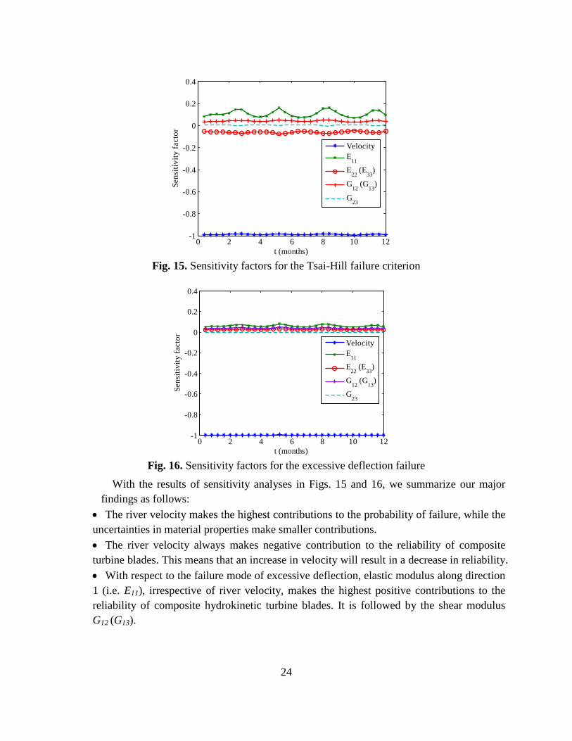
Based on this, we obtained the sensitivities factors of random variables at every time instant. Figs. 15 and 16 show sensitivity factors of the five random variables for the Tsai-Hill failure

criterion and excessive deflection, respectively.

24

0 2 4 6 8 10 12

-1

-0.8

-0.6

-0.4

-0.2

0

0.2

0.4

t (months)

Sens

itivi

ty fa

ctor

VelocityE

11

E22

(E33

)

G12

(G13

)

G23

Fig. 15. Sensitivity factors for the Tsai-Hill failure criterion

0 2 4 6 8 10 12

-1

-0.8

-0.6

-0.4

-0.2

0

0.2

0.4

t (months)

Sens

itivi

ty fa

ctor

VelocityE

11

E22

(E33

)

G12

(G13

)

G23

Fig. 16. Sensitivity factors for the excessive deflection failure

With the results of sensitivity analyses in Figs. 15 and 16, we summarize our major findings as follows:

• The river velocity makes the highest contributions to the probability of failure, while the uncertainties in material properties make smaller contributions. • The river velocity always makes negative contribution to the reliability of composite turbine blades. This means that an increase in velocity will result in a decrease in reliability. • With respect to the failure mode of excessive deflection, elastic modulus along direction 1 (i.e. E11), irrespective of river velocity, makes the highest positive contributions to the reliability of composite hydrokinetic turbine blades. It is followed by the shear modulus G12 (G13).

25

• For the failure mode of the Tsai-Hill failure criterion, E22 turns out to make negative contributions to the reliability of turbine blades while the sensitivity with respect to E11 is positive and the largest. • The shear modulus G23 always makes negligible contributions to both of the failure modes.

6. Conclusions

Using an appropriate reliability analysis method is critical for the probabilistic design of composite hydrokinetic turbine blades. In this work, we developed a simulation based time-dependent reliability model for composite hydrokinetic turbine blades. The BEM-FEM coupled method was used to get the responses of failure indicator of the Tsai-Hill failure criterion and deflections of turbine blades. The SPCE method was adopted to establish the limit-state functions, and JUR/FORM was employed to perform time-dependent reliability analysis. By incorporating these analysis methods, we evaluated the influence of uncertainties in river flow velocity and composite material properties on the performance of turbine blades.

The results illustrated that the composite hydrokinetic turbine blade has larger probability of failure for the excessive deflection than that due to the Tsai-Hill failure criterion. The former, therefore, needs to be paid more attention during the design phase.

Sensitivity analysis of random variables showed that the river flow velocity makes the highest contribution to the probability of failure of the composite hydrokinetic turbine blade for both failure modes. The sensitivity analysis of the composite material parameters showed that E11 always makes a positive contribution and is the most important composite material parameter for the reliability of turbine blades. Therefore, this parameter should be focused on during the design stage. The shear modulus G23 makes negligible contributions to the two failure modes. E22

makes a positive contribution to the reliability of turbine blades against excessive deflection while this contribution turns to be negative for the reliability against the failure mode of Tsai-Hill failure criterion. This demonstrated that the material parameters of the composite material make different contributions to the reliability of turbine blades.

Our future work includes coupling the CFD simulation with FEM to improve accuracy and applying the developed method to the reliability-based design optimization (RBDO) of composite hydrokinetic turbine blades. Fatigue reliability analysis will also be our future work.

Appendix A: MCS for time-dependent reliability analysis

The MCS for time-dependent reliability analysis involves both a stochastic process (river flow discharge) and random variables. To generate samples for the stochastic process, we discretize the time interval 0[ , ]st t

into N points. Then the samples of the normalized and

standardized river flow discharge process mD is generated by

26

mD= +mD Mςm (33)

where 1 2,( , , )TNς ς ς=ς is the vector of N independent standard normal random variables;

1 2,( ( ) ( ), , ( ))m m m m

TD D D D Nt t tm m m= m is the vector of mean values of

1 2,( ( ) ( ), , ( ))Tm m m ND t D t D t=mD ; and M is a lower triangular matrix obtained from the

covariance matrix of mD .

Let the covariance matrix of mD at the N points be N N×C , we have

( ) ( ) ( )( ) ( ) ( )

( ) ( ) ( )

1 1 1 2 1

2 1 2 2 2

1 2

, , ,

, , ,

, , ,

m m m

m m m

m m m

D D D N

D D D NN N

D N D N D N N N N

t t t t t t

t t t t t t

t t t t t t

ρ ρ ρ

ρ ρ ρ

ρ ρ ρ

×

×

=

C

(34)

Then M can be obtained by

1 TN N

−× = =C PDP MM (35)

in which D is a diagonal eigenvalue matrix of the covariance matrix N N×C , and P is the N N×

square matrix whose i-th column is the i-th eigenvector of N N×C . After samples of the stochastic process of river flow discharge are generated, they are plugged

into the limit-state functions, and then the samples (trajectories) of the limit-state functions are obtained. A trajectory is traced from the initial time to the end of the time period. Once the trajectory upcrosses the limit state, then a failure occurs; and the remaining curve will not be checked anymore. The process is illustrated in Fig. 17.

Fig. 17. A trajectory of a limit-state function

Time t

Limit state g

t1

Upcrossing: failure occurs

27

Appendix B: Computation of 1 2( , )v t t++

Madsen has derived the expression for 1 2( , )v t t++ as follows [31]

( ) ( ) ( )( ) ( ) ( )( ) ( ) ( )

1 2 1 2 1 1 1 2 2 2

1 2 1 1 1 2 2 2

2 21 2 0

( , ) ( ) / ( ) /

( ) / ( ) /

| ;

v t t f

f

f K f K dKκ

λ λ β m λ β m λ

λ λ κ m β λ m β λ

λ λ κ

++ = Ψ − Ψ −

+ Φ − Φ −

+ −∫

W

W

W W W

β

β

β β β

(36)

in which

( ) 2 2 2 21 1 2 2{exp[( 2 ) / (2 2 )]} / (2 1 )f β ρβ β β ρ p ρ= − + − −W β (37)

1 2,β ββ=[ ] represents the time-invariant reliability index at time 1t and 2t . 1 2andm m , and

1 2and ,λ λ κ are the mean values, standard deviations, and correlation coefficient of 1( )L t β

and

2( )L t β , respectively. They are calculated by the following equations [28]:

1 1 22 1 1

2 1 2 2

( )/ (1 )

( )m β ρβ ρ

m ρm β ρβ ρ

− − = = = − −

LLLLc c β

(38)

2

1 1 1 22

1 2 2

λ κλ λκλ λ λ

− = = − =

∑ L L LLLL LL LLc c c c c

(39)

where

21 12 1

221 2 2

2

1

( ) 0( ) 0

0 10 1

tt

ω ρ ρρ ω ρ

ρ ρρ ρ

=

LL LL

LLLL

c cc c

(40)

1 1 1 2 2 1 1 1 2 2( ) ( , ) ( ) ( ) ( , ) ( )T Tt t t t t t t tρ = +α C α α C α

(41)

2 1 1 2 2 1 2 1 2 2( ) ( , ) ( ) ( ) ( , ) ( )T Tt t t t t t t tρ = +α C α α C α

(42)

12 1 2 1 2 2 1 1 2 2

1 12 1 2 2 1 1 1 2 2

( ) ( , ) ( ) ( ) ( , ) ( )

( ) ( , ) ( ) ( ) ( , ) ( )

T T

T T

t t t t t t t t

t t t t t t t t

ρ = +

+ +

α C α α C α

α C α α C α

(43)

21 1 1 2 2 1 1 1 2 2

1 21 1 2 2 1 2 1 2 2

( ) ( , ) ( ) ( ) ( , ) ( )

( ) ( , ) ( ) ( ) ( , ) ( )

T T

T T

t t t t t t t t

t t t t t t t t

ρ = +

+ +

α C α α C α

α C α α C α

(44)

28

1

1 21 2

1 2 ( ) ( )

( , ) 0( , )

0 ( , )m

Y

Yn m n m

t tt t

t t

ρ

ρ+ × +

=

1 0 00

C

0

(45)

and

11 2

1 2 1 2

1 2

( ) ( )

( , ) 0

( , ) ( , ) / , 1, 2

( , )0m

Y

jj j

Y

j n m n m

t tt

t t t t t j

t tt

ρ

ρ

+ × +

∂ ∂ = ∂ ∂ = = ∂

∂

0 0 0

0

C C

0

(46)

Acknowledgements The authors gratefully acknowledge the support from the Office of Naval Research through

contract ONR N000141010923 (Program Manager - Dr. Michele Anderson) and the Intelligent Systems Center at the Missouri University of Science and Technology.

Reference [1] D.A. Brooks, The hydrokinetic power resource in a tidal estuary: The Kennebec River of the central Maine coast, Renewable Energy, 36 (2011) 1492-1501. [2] M.S. Guney, Evaluation and measures to increase performance coefficient of hydrokinetic turbines, Renewable and Sustainable Energy Reviews, 15 (2011) 3669-3675. [3] L.I. Lago, F.L. Ponta, L. Chen, Advances and trends in hydrokinetic turbine systems, Energy for Sustainable Development, 14 (2010) 287-296. [4] V.J. Ginter, J.K. Pieper, Robust gain scheduled control of a hydrokinetic turbine, IEEE Transactions on Control Systems Technology, 19 (2011) 805-817. [5] R. Hantoro, I.K.A.P. Utama, Erwandi, A. Sulisetyono, An experimental investigation of passive variable-pitch vertical-axis ocean current turbine, ITB Journal of Engineering Science, 43 B (2011) 27-40. [6] T.Y. Kam, H.M. Su, B.W. Wang, Development of glass-fabric composite wind turbine blade, Advanced Materials Research, (2011), pp. 2482-2485. [7] M.R. Motley, Y.L. Young, Performance-based design and analysis of flexible composite propulsors, Journal of Fluids and Structures, 27 (2011) 1310-1325. [8] Y.L. Young, J.W. Baker, M.R. Motley, Reliability-based design and optimization of adaptive marine structures, Composite Structures, 92 (2010) 244-253. [9] B. Kriegesmann, R. Rolfes, C. Hühne, A. Kling, Fast probabilistic design procedure for axially compressed composite cylinders, Composite Structures, 93 (2011) 3140-3149. [10] M.R. Motley, Y.L. Young, Influence of uncertainties on the response and reliability of self-adaptive composite rotors, Composite Structures, 94 (2011) 114-120.

29

[11] R.J. Pimenta, S.M.C. Diniz, G. Queiroz, R.H. Fakury, A. Galvão, F.C. Rodrigues, Reliability-based design recommendations for composite corrugated-web beams, Probabilistic Engineering Mechanics, 28 (2012) 185-193. [12] H.S. Toft, J.D. Sørensen, Reliability-based design of wind turbine blades, Structural Safety, 33 (2011) 333-342. [13] D.V. Val, L. Chernin, Reliability of tidal stream turbine blades, in: 11th International Conference on Applications of Statistics and Probability in Civil Engineering, ICASP, Zurich, 2011, pp. 1817-1822. [14] M.R. Motley, Y.L. Young, Reliability-based global design of self-adaptive marine rotors, in: ASME 2010 3rd Joint US-European Fluids Engineering Summer Meeting, FEDSM 2010, Montreal, QC, 2010, pp. 1113-1122. [15] C.D. Eamon, M. Rais-Rohani, Integrated reliability and sizing optimization of a large composite structure, Marine Structures, 22 (2009) 315-334. [16] M. Chiachio, J. Chiachio, G. Rus, Reliability in composites - A selective review and survey of current development, Composites Part B: Engineering, 43 (2012) 902-913. [17] X. Du, A. Sudjianto, Reliability-based design with the mixture of random and interval variables, Journal of Mechanical Design, Transactions of the ASME, 127 (2005), pp. 1068-1076. [18] X. Du, A. Sudjianto, W. Chen, An integrated framework for optimization under uncertainty using inverse reliability strategy, Journal of Mechanical Design, Transactions of the ASME, 126 (2004) 562-570. [19] M. Muste, K. Yu, T. Pratt, D. Abraham, Practical aspects of ADCP data use for quantification of mean river flow characteristics; Part II: Fixed-vessel measurements, Flow Measurement and Instrumentation, 15 (2004) 17-28. [20] M.Y. Otache, M. Bakir, Z. Li, Analysis of stochastic characteristics of the Benue River flow process, Chinese Journal of Oceanology and Limnology, 26 (2008) 142-151. [21] J.N. Yang, M. Shinozuka, On the first excursion probability in stationary narrow- band random vibration, Journal of Applied Mechanics, Transactions ASME, 38 Ser E (1971) 1017-1022. [22] B. Sudret, Analytical derivation of the outcrossing rate in time-variant reliability problems, Structure and Infrastructure Engineering, 4 (2008) 353-362. [23] F.M.H. Schall G, Rackwitz R., The ergodicity assumption for sea states in the reliability estimation of offshore structures. , Journal of Offshore Mechanics and Arctic Engineering, 113 (1991) 241–246. [24] S. Engelund, R. Rackwitz, C. Lange, Approximations of first-passage times for differentiable processes based on higher-order threshold crossings, Probabilistic Engineering Mechanics, 10 (1995) 53-60. [25] J. Zhang, X. Du, Time-dependent reliability analysis for function generator mechanisms, Journal of Mechanical Design, Transactions of the ASME, 133 (2011). [26] C. Andrieu-Renaud, B. Sudret, M. Lemaire, The PHI2 method: A way to compute time-variant reliability, Reliability Engineering and System Safety, 84 (2004) 75-86. [27] Z. Hu, X. Du, Reliability analysis for hydrokinetic turbine blades, Renewable Energy, 48 (2012) 251-262. [28] Z. Hu, X. Du, Time-Dependent Reliability Analysis with Joint Upcrossing Rates, Submitted to Structural and Multidisciplinary Optimization, (2011). [29] S.O. Rice, Mathematical Analysis of Random Noise, Bell System Technical Journal, 23 (1944) 282–332.

30

[30] S.O. Rice, Mathematical analysis of random noise, Bell Syst.Tech. J., 24 (1945) 146-156. [31] P.H. Madsen, and Krenk, S.,, An integral equation method for the first passage problem in random vibration, Journal of Applied Mechanics 51 (1984) 674-679. [32] E.H. Vanmarcke, On the distribution of the first-passage time for normal stationary random processes, Journal of Applied Mechanics, Transactions ASME, 42 Ser E (1975) 215-220. [33] A. Preumont, On the peak factor of stationary Gaussian processes, Journal of Sound and Vibration, 100 (1985) 15-34. [34] A. Singh, Z. Mourelatos, J. Li, Design for lifecycle cost using time-dependent reliability, Journal of Mechanical Design, Transactions of the ASME, 132 (2010) 091008. [35] V.K. Arora, G.J. Boer, A variable velocity flow routing algorithm for GCMs, Journal of Geophysical Research D: Atmospheres, 104 (1999) 30965-30979. [36] K. Schulze, M. Hunger, P. Döll, Simulating river flow velocity on global scale, Advances in Geosciences, 5 (2005) 133-136. [37] P.M. Allen, J.G. Arnold, B.W. Byars, Downstream channel geometry for use in planning-level models, Water Resources Bulletin, 30 (1994) 663-671. [38] J.J. Beersma, T.A. Buishand, Joint probability of precipitation and discharge deficits in the Netherlands, Water Resources Research, 40 (2004) 1-11. [39] H.T. Mitosek, On stochastic properties of daily river flow processes, Journal of Hydrology, 228 (2000) 188-205. [40] P.H.A.J.M. W. Wang, Van Gelder and J.K. Vrijling, Long-memory in streamflow processes of the yellow river, IWA International Conference on Water Economics, Statistics, and Finance Rethymno, Greece, July 8-10, (2005) 481-490. [41] K.O. Ronold, C.J. Christensen, Optimization of a design code for wind-turbine rotor blades in fatigue, Engineering Structures, 23 (2001) 993-1004. [42] D. Veldkamp, A probabilistic evaluation of wind turbine fatigue design rules, Wind Energy, 11 (2008) 655-672. [43] K.O. Ronold, G.C. Larsen, Reliability-based design of wind-turbine rotor blades against failure in ultimate loading, Engineering Structures, 22 (2000) 565-574. [44] K. Saranyasoontorn, L. Manuel, Design loads for wind turbines using the environmental contour method, Journal of Solar Energy Engineering, Transactions of the ASME, 128 (2006) 554-561. [45] M. Grujicic, G. Arakere, B. Pandurangan, V. Sellappan, A. Vallejo, M. Ozen, Multidisciplinary design optimization for glass-fiber epoxy-matrix composite 5 MW horizontal-axis wind-turbine blades, Journal of Materials Engineering and Performance, 19 (2010) 1116-1127. [46] C.K. Lee, Corrosion and wear-corrosion resistance properties of electroless Ni-P coatings on GFRP composite in wind turbine blades, Surface and Coatings Technology, 202 (2008) 4868-4874. [47] K. Mühlberg, Corrosion protection of offshore wind turbines - A challenge for the steel builder and paint applicator, Journal of Protective Coatings and Linings, 27 (2010) 20-32. [48] A.L. Araújo, C.M. Mota Soares, C.A. Mota Soares, J. Herskovits, Optimal design and parameter estimation of frequency dependent viscoelastic laminated sandwich composite plates, Composite Structures, 92 (2010) 2321-2327. [49] Y.X. Zhang, C.H. Yang, Recent developments in finite element analysis for laminated composite plates, Composite Structures, 88 (2009) 147-157.

31

[50] O.L.H. Martin, Aerodynamics of wind turbines, Second edition, Earthscan, Sterling, VA., 2008. [51] Blade Tidal, Demonstration version, GL Garrad Hassan, www.gl-garradhassan.com. [52] M.S. Eldred, J. Burkardt, Comparison of non-intrusive polynomial chaos and stochastic collocation methods for uncertainty quantification, in: 47th AIAA Aerospace Sciences Meeting including the New Horizons Forum and Aerospace Exposition , art. no. 2009-0976 2009. [53] B. Sudret, Global sensitivity analysis using polynomial chaos expansions, Reliability Engineering and System Safety, 93 (2008) 964-979. [54] M.S. Eldred, Recent advances in non-intrusive polynomial chaos and stochastic collocation methods for uncertainty analysis and design, in: 50th AIAA/ASME/ASCE/AHS/ASC Structures, Structural Dynamics and Materials Conference , art. no. 2009-2274 2009. [55] W. Chen, K.-L. Tsui, J.K. Allen, F. Mistree, Integration of the response surface methodology with the compromise decision support problem in developing a general robust design procedure, in: American Society of Mechanical Engineers, Design Engineering Division (Publication) DE 82 (1), pp. 485-492 1995. [56] S.K. Choi, R.V. Grandhi, R.A. Canfield, Reliability-based structural design, Springer, 2007.